Braneworld cosmological solutions and their stability

Abstract

We consider cosmological solutions and their stability with respect to homogeneous and isotropic perturbations in the braneworld model with the scalar-curvature term in the action for the brane. Part of the results are similar to those obtained by Campos and Sopuerta for the Randall–Sundrum braneworld model. Specifically, the expanding de Sitter solution is an attractor, while the expanding Friedmann solution is a repeller. In the braneworld theory with the scalar-curvature term in the action for the brane, static solutions with matter satisfying the strong energy condition exist not only with closed spatial geometry but also with open and flat ones even in the case where the dark-radiation contribution is absent. In a certain range of parameters, static solutions are stable with respect to homogeneous and isotropic perturbations.

PACS number(s): 04.50.+h

1 Introduction

Braneworld models have become quite popular in the high-energy and gravitational physics during last several years. There are at least three reasons for this. Firstly, most of the brane models, in particular, the Randall–Sundrum model [1], are inspired directly by the popular string theory (specifically, by the Hor̆ava–Witten model [2]) and represent an interesting alternative for compactification of extra spatial dimensions. Secondly, there remains a possibility of solving the mass-hierarchy problem in the context of large extra dimensions (see [3, 1]). And thirdly, it has been shown that models with non-compact extra dimensions and branes can be consistent with the current gravity experiments.

Braneworld models also turned out to be consistent with modern cosmology, at the same time exhibiting new specific features. First of all, this concerns the braneworld models of “dark energy,” or of the currently observed acceleration of the universe (see [4] in this respect), but this is also true with respect to the early stages of cosmological evolution such as inflation (see, e.g., [5]).

A broad class of cosmological solutions in braneworld theory was systematically analyzed by Campos and Sopuerta [6] using convenient phase space variables similar to those introduced in [7]. These authors gave a complete description of stationary points in an appropriately chosen phase space of the cosmological setup and investigated their stability with respect to homogeneous and isotropic perturbations. The authors worked in the frames of the Randall–Sundrum braneworld theory without the scalar-curvature term in the action for the brane. In this paper, we are going to extend this analysis by investigating the case where this term is present in the action.

The scalar-curvature term for the brane was introduced in [8] (see also [9]) as a method of making gravity on the brane effectively four-dimensional even in the flat infinite bulk space. The corresponding cosmological models were initiated in [9, 10]. The necessity of this term on the brane arises when one considers the complete effective action of the theory (see, e.g., [11]). From this viewpoint, the term with brane tension represents the zero-order term in the expansion of the total action for the brane in powers of curvature of the induced metric, while the next term in the action for the brane is exactly the scalar-curvature Hilbert–Einstein term. From another (complementary) viewpoint [8], this contribution is induced as a quantum correction to the effective action for the brane gravity after one takes into account the quantum character of the matter confined to the brane.

In this paper, we will show that the presence of the scalar-curvature term in the action for the brane enlarges the class of cosmological solutions, in particular, it allows for the existence of static cosmological solutions with ordinary matter content even in the case of spatially flat or open cosmology, a specific feature of the braneworld cosmology that was also noted in [6, 12, 4]. In the Randall–Sundrum model, flat or open static universe with ordinary matter requires the presence of the negative dark-radiation term, while, in the model with scalar-curvature term in the action for the brane to be discussed in this paper, the presence of dark radiation may be not necessary.

The paper is organized as follows:   In Sec. 2, we introduce the basic equations describing the theory with one brane in the five-dimensional bulk space. Then, in Sec. 3, we introduce a method for the investigation of static solutions. Using this method, we describe both the general-relativity case and the case of braneworld theory that contains the scalar-curvature term in the action for the brane. In the partial case of spatially flat universe, we determine the range of parameters where static solutions exist and where they are stable with respect to homogeneous and isotropic perturbations. In Sec. 4, we develop an approach which is used to describe non-static solutions, and apply it to the braneworld theory under investigation. In Sec. 5, we return to the issue of static solutions with arbitrary spatial curvature using conveniently chosen variables. Finally, in Sec. 6, we present our conclusions.

2 Basic equations

In this paper, we consider the case where the braneworld is the time-like boundary of a five-dimensional purely gravitational Lorentzian space (bulk), which is equivalent to the case of a brane embedded in the bulk with $\mathbb{Z}_{2}$ symmetry of reflection with respect to the brane. The theory is described by the action [9]:

$$S=-M^{3}\left[\int_{\rm bulk}(\mathcal{R}-2\Lambda_{\rm b})-2\int_{\rm brane}K\right]-\int_{\rm brane}(m^{2}R-2\sigma)+\int_{\rm brane}L(h_{ab},\phi)\,.$$ (2.1)

Here, $\mathcal{R}$ is the scalar curvature of the metric $g_{ab}$ in the five-dimensional bulk, and $R$ is the scalar curvature of the induced metric $h_{ab}=g_{ab}-n_{a}n_{b}$ on the brane, where $n^{a}$ is the vector field of the inner unit normal to the brane, and the notation and conventions of [13] are used. The quantity $K=K_{ab}h^{ab}$ is the trace of the symmetric tensor of extrinsic curvature $K_{ab}=h^{c}_{a}\nabla_{c}n_{b}$ on the brane. The symbol $L(h_{ab},\phi)$ denotes the Lagrangian density of the four-dimensional matter fields $\phi$ whose dynamics is restricted to the brane so that they interact only with the induced metric $h_{ab}$. All integrations over the bulk and brane are taken with the natural volume elements $\sqrt{-g}d^{5}x$ and $\sqrt{-h}d^{4}x$, respectively, where $g$ and $h$ are the determinants of the matrices of components of the corresponding metrics in a coordinate basis. The symbols $M$ and $m$ denote, respectively, the five- and four-dimensional Planck masses, $\Lambda_{\rm b}$ is the bulk cosmological constant, and $\sigma$ is the brane tension.

The term containing the scalar curvature of the induced metric on the brane with the coupling $m^{2}$ in action (2.1) was originally absent from braneworld models. However, very soon it became clear that this term is qualitatively essential for describing the braneworld dynamics and, moreover, it is inevitably generated as a quantum correction to the matter action in (2.1) — in the spirit of an idea that goes back to Sakharov [14] (see also [15]). Note that the effective action for the brane typically involves an infinite number of terms of higher order in curvature (this was pointed out in [9] for the case of braneworld theory; a similar situation in the context of the AdS/CFT correspondence is described in [11]). In this paper, we retain only the terms linear in curvature. The effects of the curvature term on the brane in linear approximation were studied in [8, 16], where it was shown that it leads to four-dimensional law of gravity on sufficiently small scales. The presence of this term also leads to qualitatively new features in cosmology, as demonstrated, in particular, in [9, 4]. For some recent reviews of the results connected with the induced-gravity term in the brane action, one may look into [17].

Variation of action (2.1) gives us the equations describing the dynamics in the bulk

$$\mathcal{G}_{ab}+\Lambda_{\rm b}g_{ab}=0\,,$$ (2.2)

and on the brane

$$m^{2}G_{ab}+\sigma h_{ab}=\tau_{ab}+M^{3}(K_{ab}-Kh_{ab})\,.$$ (2.3)

The second equation generalizes the Israel junction conditions [18] and the corresponding equation of the Randall–Sundrum model to the presence of the scalar-curvature term on the brane ($m\neq 0$).

One can consider the Gauss identity

$$R_{abc}{}^{d}=h_{a}{}^{f}h_{b}{}^{g}h_{c}{}^{k}h^{d}{}_{j}{\cal R}_{fgk}{}^{j}+K_{ac}K_{b}{}^{d}-K_{bc}K_{a}{}^{d}\,,$$ (2.4)

and, following the original procedure of [19], contract it once on the brane using equations (2.2) and (2.3). In this way, one obtains the effective equation on the brane that generalizes the result of [19] to the presence of the brane curvature term:

$$G_{ab}+\Lambda_{\rm eff}h_{ab}=\frac{1}{M_{\rm P}^{2}}\tau_{ab}+\frac{1}{1+2\sigma m^{2}/3M^{6}}\left(M^{6}Q_{ab}-W_{ab}\right)\,,$$ (2.5)

where

$$\Lambda_{\rm eff}=\frac{\Lambda_{\rm RS}}{1+2\sigma m^{2}/3M^{6}}\,,\quad\Lambda_{\rm RS}=\frac{\Lambda_{\rm b}}{2}+\frac{\sigma^{2}}{3M^{6}}\,,\quad M_{\rm P}^{2}=m^{2}+\frac{3M^{6}}{2\sigma}\,,$$ (2.6)

$$Q_{ab}=\frac{1}{3}EE_{ab}-E_{ac}E^{c}{}_{b}+\frac{1}{2}\left(E_{cd}E^{cd}-\frac{1}{3}E^{2}\right)h_{ab}$$ (2.7)

is the quadratic expression with respect to the ‘bare’ Einstein equation $E_{ab}\equiv m^{2}G_{ab}-\tau_{ab}$ on the brane, $E=h^{ab}E_{ab}$, and $W_{ab}\equiv h^{c}{}_{a}h^{e}{}_{b}W_{cdef}n^{d}n^{f}$ is a projection of the bulk Weyl tensor $W_{abcd}$ to the brane. The limit of $m\to 0$ leads us to the original result of [19].

Contracting Eq. (2.5) once again, one obtains the following scalar equation on the brane:

$$M^{6}(R-2\Lambda_{\rm b})+(m^{2}G_{ab}+\sigma h_{ab}-\tau_{ab})(m^{2}G^{ab}+\sigma h^{ab}-\tau^{ab})-\frac{1}{3}(m^{2}R-4\sigma+\tau)^{2}=0\,,$$ (2.8)

where $\tau=\tau_{ab}h^{ab}$. It is argued in [20] that, if one is interested only in the evolution on the brane and if no additional boundary or regularity conditions are specified in the bulk (as often is the case), then one is left only with this scalar equation. Having obtained a solution of (2.8), one can integrate the gravitational equations in the bulk using, for example, Gaussian normal coordinates [19, 20].

The brane filled by a homogeneous and isotropic ideal fluid is described by the Friedmann–Robertson–Walker (FRW) metric

$$ds^{2}=-dt^{2}+a^{2}(t)\left[\frac{dr^{2}}{1-\kappa r^{2}}+r^{2}d\Omega^{2}\right]\,,$$ (2.9)

where $\kappa=-1$, $0$, or $+1$. The stress–energy tensor of the ideal fluid takes the form

$$\tau_{ab}=(\rho+p)u_{a}u_{b}+ph_{ab}\,,$$ (2.10)

where $\rho$ is the energy density, and $p$ is the pressure. In this paper, we assume a simple equation of state $p=w\rho$, where $w$ is constant.

Equation (2.8) leads to the following cosmological equation in the braneworld theory:

$$9M^{6}\left[\frac{\ddot{a}}{a}+H^{2}+\frac{\kappa}{a^{2}}-\frac{\Lambda_{\rm b}}{3}\right]+\left[\rho(1+3w)-2\sigma+6m^{2}\frac{\ddot{a}}{a}\right]\left[\rho+\sigma-3m^{2}\left(H^{2}+\frac{\kappa}{a^{2}}\right)\right]=0\,,$$ (2.11)

where $H\equiv\dot{a}/a$ is the Hubble parameter. After multiplying this equation by $a^{3}\dot{a}$ and using the conservation of energy

$$\dot{\rho}+3H(\rho+p)=0\,,$$ (2.12)

one can integrate Eq. (2.11) and obtain the first-order differential equation [20, 4]

$$m^{4}\left(H^{2}+\frac{\kappa}{a^{2}}-\frac{\rho+\sigma}{3m^{2}}\right)^{2}=M^{6}\left(H^{2}+\frac{\kappa}{a^{2}}-\frac{\Lambda_{\rm b}}{6}-\frac{C}{a^{4}}\right)\,,$$ (2.13)

where $C$ is the integration constant corresponding to the black-hole mass of the Schwarzschild–(anti)-de Sitter solution in the bulk and associated with what is called “dark radiation.”

Equation (2.13) can be solved with respect to the Hubble parameter:

$$H^{2}+\frac{\kappa}{a^{2}}=\frac{\rho+\sigma}{3m^{2}}+\frac{2}{\ell^{2}}\left[1\pm\sqrt{1+\ell^{2}\left(\frac{\rho+\sigma}{3m^{2}}-\frac{\Lambda_{\rm b}}{6}-\frac{C}{a^{4}}\right)}\right]\,,$$ (2.14)

where $\ell=2m^{2}/M^{3}$ is the crossover length scale characterizing the theory. The ‘$\pm$’ signs give the two different branches of braneworld solutions which, to some extent, are connected with the two different ways in which the Schwarzschild–(anti)-de Sitter bulk space is bounded by the brane: the inner normal to the brane can point either in the direction of increasing or decreasing of the bulk radial coordinate. Following [4], we refer to the model with the lower sign (‘$-$’) as to BRANE1, and to that with the upper sign (‘$+$’) as to BRANE2.

In the formal limit of $m\to 0$, the BRANE1 model reduces to the well-known expression obtained in the Randall–Sundrum case

$$H^{2}+\frac{\kappa}{a^{2}}=\frac{(\rho+\sigma)^{2}}{9M^{6}}+\frac{\Lambda_{\rm b}}{6}+\frac{C}{a^{4}}\,,$$ (2.15)

while the BRANE2 model does not exist in this limit. This can be viewed as a simple consequence of the fact that Eq. (2.13), being quadratic with respect of the Hubble parameter $H$ in the case $m\neq 0$, reduces to a linear equation with respect to $H$ in the formal limit $m\to 0$.

3 Static solutions

We proceed to the investigation of static solutions in the braneworld theory. First, we review the situation in the general relativity theory, where the static Einstein’s universe is known to be unstable. We apply the same method for the investigation of the stability of static solutions in the braneworld theory and demonstrate new possibilities arising in this theory. Firstly, unlike general relativity, the braneworld theory admits static solutions even in the case of spatially flat or open universe, which, in the context of the Randall–Sundrum model, was also noted in [12]. In the Randall–Sundrum model, static spatially flat or open universes with matter satisfying the strong energy condition are possible only with negative value of the dark-radiation constant $C$, while, in the presence of the scalar-curvature term in the action for the brane, a spatially flat or open universe can be static even when this constant is zero. Secondly, these solutions can be stable in certain region of parameters.

3.1 The case of general relativity

In this section, we review the situation in the general relativity theory with the standard action

$$S_{\rm GR}=-\frac{1}{16\pi G}\int(R-2\Lambda)\sqrt{-g}d^{4}x+\int L_{\rm matter}\sqrt{-g}d^{4}x$$ (3.1)

and describe our method for investigation of the stability of static solutions on the example of this theory. A homogenous and isotropic universe with density $\rho$ and pressure $p=w\rho$ is described by the Friedmann equations

$$H^{2}+\frac{\kappa}{a^{2}}=\frac{8\pi G\rho}{3}+\frac{\Lambda}{3}\,,$$ (3.2)

$$\frac{\ddot{a}}{a}=-\frac{4\pi G\rho}{3}(1+3w)+\frac{\Lambda}{3}\,,$$ (3.3)

giving the following conditions of static solution:

$$\frac{\kappa}{a_{0}^{2}}=\frac{8\pi G\rho_{0}}{3}+\frac{\Lambda}{3}\,,$$ (3.4)

$$\frac{4\pi G\rho_{0}}{3}(1+3w)-\frac{\Lambda}{3}=0\,.$$ (3.5)

Introducing small homogeneous deviations from stationarity,

$$a=a_{0}(1-\epsilon)\,,\quad\epsilon=\epsilon(t)\ll 1\,,$$ (3.6)

and linearizing the Friedmann equations (3.2) and (3.3) with respect to the small quantity $\epsilon(t)$, we have:

$$\frac{2\kappa\epsilon}{a_{0}^{2}}=\frac{8\pi G(\rho-\rho_{0})}{3}\,,$$ (3.7)

$$\ddot{\epsilon}=W\epsilon,\quad W=\frac{\kappa(1+3w)}{a_{0}^{2}}\,.$$ (3.8)

We note that the weak energy condition and casuality requirements restrict the value of $w$ to lie in the interval $w\in[-1,+1]$ (see, e.g., [21]) and, as a result, $\kappa=+1$. Taking this into account, one can see from (3.8) that the static solution in this theory is unstable for $w\in\left[-\frac{1}{3},1\right]$, and stable for $w\in\left(-1,-\frac{1}{3}\right)$.

3.2 The case of braneworld theory

One can use the method outlined in the previous section to investigate the braneworld theory. In this section, we find (analytically and graphically) the regions of existence of static solutions in the parameter space and then further restrict the space of parameters by the requirement that the described theory be physically compatible with the observations.

3.2.1 Static solutions and their perturbation

In the static case, equations (2.11) and (2.13) give

$$9M^{6}\left(\frac{\kappa}{a^{2}}-\frac{\Lambda_{\rm b}}{3}\right)+\left[\rho(1+3w)-2\sigma\right]\left(\rho+\sigma-3m^{2}\frac{\kappa}{a^{2}}\right)=0$$ (3.9)

and

$$m^{4}\left(\frac{\kappa}{a^{2}}-\frac{\rho+\sigma}{3m^{2}}\right)^{2}=M^{6}\left(\frac{\kappa}{a^{2}}-\frac{\Lambda_{\rm b}}{6}-\frac{C}{a^{4}}\right)\,,$$ (3.10)

respectively. One should note that Eq. (3.10) cannot be obtained by integrating Eq. (2.11) in the static case because, before integration, Eq. (2.11) is multiplied by $\dot{a}$, which, in this case, is identically zero. Nevertheless, it can be obtained from the original equations on the brane (2.3) considering the embedding of the brane in the bulk. In fact, this equation determines the value of the black-hole constant $C$ for which a solution of (3.9) is embeddable in the Schwarzschild–(anti)-de Sitter bulk.

Looking for static solutions and investigating their stability, we proceed as in the previous case of general relativity. First, we solve Eq. (2.11) with respect to $\ddot{a}/a$ for $\dot{a}=0$:

$$\frac{\ddot{a}}{a}=-\frac{9M^{6}\left(\frac{\kappa}{a^{2}}-\frac{\Lambda_{\rm b}}{3}\right)+\left[\rho(1+3w)-2\sigma\right]\left(\rho+\sigma-3m^{2}\frac{\kappa}{a^{2}}\right)}{9M^{6}+6m^{2}\left(\rho+\sigma-3m^{2}\frac{\kappa}{a^{2}}\right)}\,.$$ (3.11)

Studying homogeneous perturbations of this solution, we set $\dot{a}=0$ as the initial condition. If a solution is stable (unstable) with respect to such perturbations, it will also be stable (unstable) with respect to more generic perturbations with $\dot{a}\neq 0$. Thus, we assume that the relation between $\rho$ and $a$ is given by Eq. (3.10) at the initial moment of time.

We express the energy density $\rho$ through $a$ using Eq. (3.10),

$$\rho=-\sigma+3m^{2}\frac{\kappa}{a^{2}}\mp 3M^{3}\sqrt{\frac{\kappa}{a^{2}}-\frac{\Lambda_{\rm b}}{6}-\frac{C}{a^{4}}}\,,$$ (3.12)

and substitute it to (3.11):

$$\frac{\ddot{a}}{a}=\frac{A_{1}}{9M^{6}\mp 18m^{2}M^{3}\sqrt{\frac{\kappa}{a^{2}}-\frac{\Lambda_{\rm b}}{6}-\frac{C}{a^{4}}}}\,,$$ (3.13)

where

$$A_{1}=-9M^{6}\left(\frac{\kappa}{a^{2}}-\frac{\Lambda_{\rm b}}{3}\right)\pm 3M^{3}A_{2}\sqrt{\frac{\kappa}{a^{2}}-\frac{\Lambda_{\rm b}}{6}-\frac{C}{a^{4}}}\,,$$ (3.14)

$$A_{2}=-3\sigma(1+w)+3(1+3w)m^{2}\frac{\kappa}{a^{2}}\mp 3(1+3w)M^{3}\sqrt{\frac{\kappa}{a^{2}}-\frac{\Lambda_{\rm b}}{6}-\frac{C}{a^{4}}}\,.$$ (3.15)

After that, we introduce the perturbation of the static solution

$$a=a_{0}(1-\epsilon)\,,\quad\epsilon(t)\ll 1\,,$$ (3.16)

where $a_{0}$ is a stationary solution of (3.13), and expand Eq. (3.13) around the stationary point:

$$\ddot{\epsilon}=W\epsilon\,,$$ (3.17)

where

$$W=\frac{B_{1}}{1\pm\frac{2m^{2}}{M^{3}}\sqrt{\frac{\kappa}{a_{0}^{2}}-\frac{\Lambda_{\rm b}}{6}-\frac{C}{a_{0}^{4}}}}\,,$$ (3.18)

$$\begin{array}[]{l}\displaystyle B_{1}=\frac{2\kappa}{a_{0}^{2}}+(1+3w)\left(\frac{2\kappa}{a_{0}^{2}}-\frac{4C}{a_{0}^{4}}\right)\mp B_{2}\pm B_{3}\pm B_{4}\,,\vskip 3.0pt plus 1.0pt minus 1.0pt\\ \displaystyle B_{2}=\frac{\sigma(1+w)}{M^{3}\sqrt{\frac{\kappa}{a_{0}^{2}}-\frac{\Lambda_{\rm b}}{6}-\frac{C}{a_{0}^{4}}}}\left(\frac{\kappa}{a_{0}^{2}}-\frac{2C}{a_{0}^{4}}\right)\,,\vskip 3.0pt plus 1.0pt minus 1.0pt\\ \displaystyle B_{3}=\frac{m^{2}}{M^{3}}\frac{2\kappa}{a_{0}^{2}}(1+3w)\sqrt{\frac{\kappa}{a_{0}^{2}}-\frac{\Lambda_{\rm b}}{6}-\frac{C}{a_{0}^{4}}}\,,\vskip 3.0pt plus 1.0pt minus 1.0pt\\ \displaystyle B_{4}=\frac{m^{2}}{M^{3}}\frac{\kappa}{a_{0}^{2}}(1+3w)\frac{\frac{\kappa}{a_{0}^{2}}-\frac{2C}{a_{0}^{4}}}{\sqrt{\frac{\kappa}{a_{0}^{2}}-\frac{\Lambda_{\rm b}}{6}-\frac{C}{a_{0}^{4}}}}\,.\end{array}$$ (3.19)

The lower and upper signs in these equations refer to the BRANE1 and BRANE2 models, respectively.

It can also be noted [4] that, unlike the general relativity theory, the braneworld theory allows for empty ($\rho=p=0$) static solutions. The radius (scale factor) of such a universe is given by the expression [4]

$$a^{2}=\frac{\kappa}{\Lambda_{\rm RS}}\left(\frac{3}{2}+\frac{\sigma m^{2}}{M^{6}}\right)\,.$$ (3.20)

The spatially flat case requires $\Lambda_{\rm RS}=0$.

3.2.2 Physical restrictions on the constants of the theory

Observations indicate that, at the present cosmological epoch, our universe expands with acceleration, so that the simplest asymptotic condition for such a universe is that the energy density will decrease monotonically to zero. Thus, we can consider the low-energy behavior of the theory as $\rho\rightarrow 0$:

$$H^{2}+\frac{\kappa}{a^{2}}=C_{1}+C_{2}\rho\,,\quad\qquad C_{1}>0\,,\quad C_{2}>0\,,$$ (3.21)

which is valid under the condition

$$\frac{\ell^{2}\rho}{3m^{2}}\ll 1+\ell^{2}\left(\frac{\sigma}{3m^{2}}-\frac{\Lambda_{\rm b}}{6}\right)\,,$$ (3.22)

and where we have assumed that the dark-radiation term (with the constant $C$ in (2.14)) has negligible contribution. Assuming regime (3.21) is realized today, we can write the following minimal physical restrictions on the constants of the theory:

BRANE1: The inequalities

$$C_{1}\equiv\frac{\sigma}{3m^{2}}+\frac{2}{\ell^{2}}\left[1-\sqrt{1+\ell^{2}\left(\frac{\sigma}{3m^{2}}-\frac{\Lambda_{\rm b}}{6}\right)}\right]>0$$ (3.23)

and

$$C_{2}\equiv\frac{1}{3m^{2}}\left[1-\frac{1}{\sqrt{1+\ell^{2}\left(\frac{\sigma}{3m^{2}}-\frac{\Lambda_{\rm b}}{6}\right)}}\right]>0$$ (3.24)

give

$$\sigma>0\,,\quad\sigma>\frac{\Lambda_{\rm b}m^{2}}{2}\,,\quad\Lambda_{\rm RS}\equiv\frac{\Lambda_{\rm b}}{2}+\frac{\sigma^{2}}{3M^{6}}>0\,.$$ (3.25)

BRANE2: The inequalities

$$C_{1}\equiv\frac{\sigma}{3m^{2}}+\frac{2}{\ell^{2}}\left[1+\sqrt{1+\ell^{2}\left(\frac{\sigma}{3m^{2}}-\frac{\Lambda_{\rm b}}{6}\right)}\right]>0$$ (3.26)

and

$$C_{2}\equiv\frac{1}{3m^{2}}\left[1+\frac{1}{\sqrt{1+\ell^{2}\left(\frac{\sigma}{3m^{2}}-\frac{\Lambda_{\rm b}}{6}\right)}}\right]>0$$ (3.27)

imply

$$\sigma>-\frac{6m^{2}}{\ell^{2}}\,,\quad\sigma>\frac{\Lambda_{\rm b}m^{2}}{2}-\frac{3m^{2}}{\ell^{2}}\,.$$ (3.28)

From these relations, one can see that BRANE2 model with the asymptotic conditions (3.21), in principle, can have negative brane tension, while the tension of the BRANE1 model is restricted to be positive.

The physical restrictions formulated above are necessary for a reasonable braneworld theory with the asymptotic limit (3.21) reached today, but they are certainly far from being sufficient for the consistency of a braneworld model with all cosmological observations (cosmic microwave background, big-bang nucleosynthesis, etc). This important issue, which, in fact, constitutes the main subject of investigations in the braneworld theory, clearly lies beyond the scope of the present paper and will be considered in our future publications. At the moment, one can only note that the values of the constants $C_{1}$ and $C_{2}$ in a braneworld that today evolves in regime (3.21) are roughly constrained by the values of the detected cosmological constant and gravitational coupling, respectively, as

$$C_{1}\simeq 0.7H_{0}^{2}\,,\qquad C_{2}\simeq\frac{8\pi G_{\rm N}}{3}\,,$$ (3.29)

where $H_{0}\approx 73\,{\rm km/sec}\cdot{\rm Mpc}$ is the current value of the Hubble parameter, and $G_{\rm N}$ is Newton’s constant. With these constraints, there remains a considerable freedom in the parameter space of the theory, which is to be further restricted by a more careful analysis.

If condition (3.22) is not satisfied today, then regime (3.21) has not yet been reached, and one should turn to the general evolution equation (2.14), which has a rather rich and interesting phenomenology for modeling dark energy [4, 22]. For example, the current acceleration of the universe expansion may be described by a braneworld model which has $C_{1}=0$ in the asymptotic expansion (3.21). According to this model, the current acceleration of the cosmological expansion is temporary, and the future evolution proceeds in a matter-dominated regime (see [4] for more details). Another interesting example is the model of loitering braneworld [23], which can be realised even in the spatially flat universe. It is the negative dark radiation (the constant $C$ in Eq. (2.14)) which plays the crucial role in the dynamics of this model and which, therefore, also needs to be constrained by cosmological observations.

3.2.3 Stability of the spatially flat static solutions

For $\kappa=0$, our equations (3.9), (3.10) and (3.18) simplify to

$${}-3M^{6}\Lambda_{\rm b}+\left[\rho(1+3w)-2\sigma\right]\cdot\left(\rho+\sigma\right)=0\,,$$ (3.30)

$$(\rho+\sigma)^{2}={}-9M^{6}\left(\frac{\Lambda_{\rm b}}{6}+\frac{C}{a^{4}}\right)$$ (3.31)

and

$$W=\frac{1}{1+\frac{2m^{2}}{3M^{6}}(\rho_{0}+\sigma)}\left[-(1+3w)\frac{4C}{a_{0}^{4}}+\frac{3\sigma(1+w)}{\rho_{0}+\sigma}\frac{2C}{a_{0}^{4}}\right]\,,$$ (3.32)

respectively.

Introducing the dimensionless parameters

$$x=\frac{\rho_{0}\ell^{2}}{6m^{2}}=\frac{2m^{2}\rho_{0}}{3M^{6}}\,,\quad y=\frac{\sigma\ell^{2}}{6m^{2}}=\frac{2m^{2}\sigma}{3M^{6}}\,,\quad z=\frac{\Lambda_{\rm b}\ell^{2}}{6}=\frac{2m^{4}\Lambda_{\rm b}}{3M^{6}}\,,$$ (3.33)

we can express the quantities that we used before in their terms. Since only two of these parameters are independent, it is convenient to express the relevant quantities in terms of $x$ and $y$. We have

$$z=\frac{1}{2}(x+y)\left[(1+3w)x-2y\right]\,,$$ (3.34)

$$\frac{C}{a_{0}^{4}}=-\frac{3M^{6}}{8m^{4}}(1+w)x(x+y)\,,$$ (3.35)

$$W=\frac{3M^{6}}{4m^{4}}(1+w)x\frac{2(1+3w)x-(1-3w)y}{1+x+y}\,.$$ (3.36)

Taking into account the physical restrictions (3.25) and (3.28) and equations (3.34) and (3.36), we can indicate the domains of existence of static solutions (both stable and unstable) in the $(x,y)$ plane.

The natural condition $\rho_{0}>0$ leads to the restriction $x>0$.

For BRANE1, restrictions (3.25) additionally give

$$y>0\,,\quad 4y>(x+y)\left[(1+3w)x-2y\right]\,,\quad(1+3w)x>(1-3w)y\,.$$ (3.37)

For BRANE2, restrictions (3.28) additionally give

$$y>-1\,,\quad 4y+2>(x+y)\left[(1+3w)x-2y\right]\,.$$ (3.38)

The corresponding domains are shown below in Figs. 1 and 2 for the two important cases $w=0$ and $w=1/3$. The shaded regions in these figures correspond to unstable static solutions ($W>0$), and the dotted regions correspond to stable static solutions ($W\leq 0$). In general, stable static solutions exist only for the BRANE2 model in the case $w<1/3$.

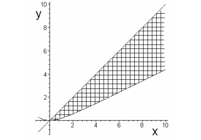
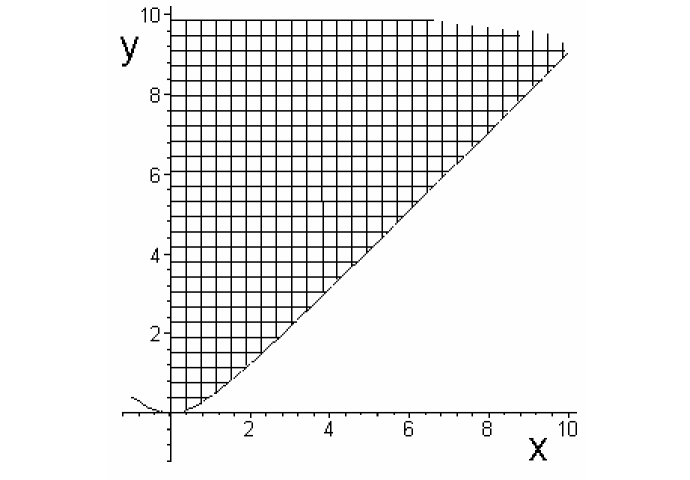
Figure 1: BRANE1, $w=0$ (left) and $w=1/3$ (right). The shaded regions indicate the physically allowable parameters, corresponding to unstable static solutions.

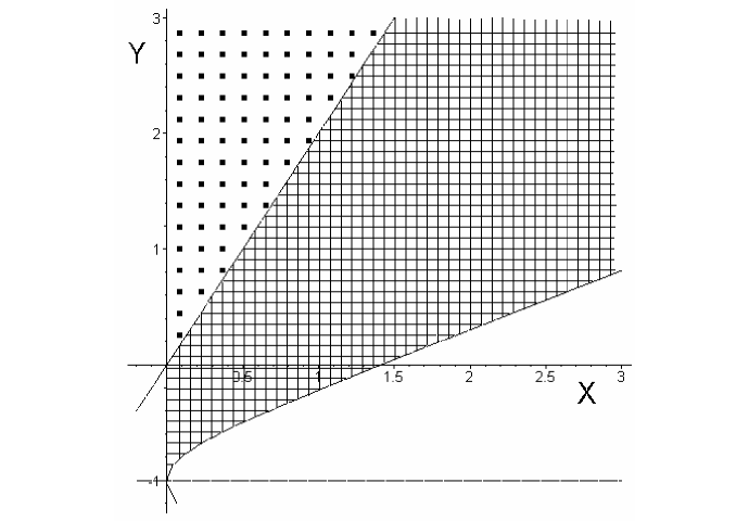
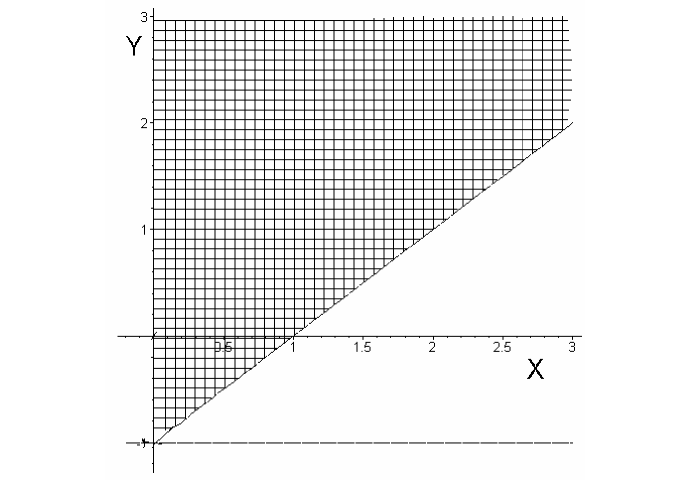
Figure 2: BRANE2, $w=0$ (left) and $w=1/3$ (right). The shaded regions of the physically allowable parameters correspond to unstable static solutions, and the dotted region corresponds to stable static solutions.

It also follows from (3.35) that spatially flat static solutions with matter satisfying the strong energy condition can exist in the BRANE2 model with $C=0$, i.e., with zero dark-radiation term, in contrast with the Randall–Sundrum model, where spatially flat or open static solutions require negative dark-radiation term. This difference is connected with the fact that the physically admissible range of parameters in the Randall–Sundrum model requires positive brane tension while, in the presence of the scalar-curvature term in the action for the brane, this restriction is weakened, and negative brane tensions are also allowed. As follows from (3.35), the condition $C=0$ is equivalent to $x+y=0$, and the region with negative $y$ in the admissible domain of parameters allowing for this condition can be seen in Fig. 2.

Stability conditions for a spatially non-flat universe ($\kappa\neq 0$) are further considered by a different method in Sec. 5.

4 Non-static solutions

In this section, we describe non-static solutions of the braneworld theory under investigation and also determine their stability. To do this, we use a set of convenient phase-space variables similar to those introduced in [6, 7]. The critical points of the system of differential equations in the space of these variables describe interesting non-static solutions. A method for evaluating the eigenvalues of the critical points of the Friedmann and Bianchi models was introduced by Goliath and Ellis [7] and further used in the analysis by Campos and Sopuerta [6] of the Randall–Sundrum braneworld theory. In this section, we extend their investigation to the case where the scalar-curvature term is also present in the action for the brane, but we restrict ourselves to the homogeneous and isotropic cosmology.

4.1 The case of the Randall–Sundrum braneworld model

In this subsection, we briefly describe the method and results of [6], where the model with $m=0$ was under consideration. After setting $m=0$, Eqs. (2.11) and (2.14) turn to

$$9M^{6}\left[\frac{\ddot{a}}{a}+H^{2}+\frac{\kappa}{a^{2}}-\frac{\Lambda_{\rm b}}{3}\right]+[\rho(1+3w)-2\sigma](\rho+\sigma)=0$$ (4.1)

and

$$H^{2}+\frac{\kappa}{a^{2}}=\frac{(\rho+\sigma)^{2}}{9M^{6}}+\frac{C}{a^{4}}+\frac{\Lambda_{\rm b}}{6}\,,$$ (4.2)

respectively. Here, for simplicity, we consider the case $C>0$. The last equation can be written as follows:

$$H^{2}=\frac{2\sigma}{9M^{6}}\rho\left(1+\frac{\rho}{2\sigma}\right)-\frac{\kappa}{a^{2}}+\frac{C}{a^{4}}+\frac{1}{3}\left(\frac{\Lambda_{\rm b}}{2}+\frac{\sigma^{2}}{3M^{6}}\right)\,.$$ (4.3)

Using the definition of the four-dimensional cosmological constant

$$\Lambda_{\rm RS}=\frac{\Lambda_{\rm b}}{2}+\frac{\sigma^{2}}{3M^{6}}\,,$$ (4.4)

which is proportional to the Randall–Sundrum constraint [1], we introduce the notation similar to those of [6]:

$$\Omega_{\rho}=\frac{2\sigma\rho}{9M^{6}H^{2}}\,,\quad\Omega_{k}=-\frac{\kappa}{a^{2}H^{2}}\,,\quad\Omega_{\Lambda}=\frac{\Lambda_{\rm RS}}{3H^{2}}\,,\quad\Omega_{\lambda}=\frac{\rho^{2}}{9M^{6}H^{2}}\,,\quad\Omega_{C}=\frac{C}{a^{4}H^{2}}\,.$$ (4.5)

The authors of [6] work in the five-dimensional $\Omega$-space $(\Omega_{\rho},\Omega_{k},\Omega_{\Lambda},\Omega_{\lambda},\Omega_{C})$. However, the $\Omega$ parameters are not all independent since they are related by the condition

$$\Omega_{\rho}+\Omega_{k}+\Omega_{\Lambda}+\Omega_{\lambda}+\Omega_{C}=1\,.$$ (4.6)

Taking this constraint into account leaves us with a four-dimensional space and only four eigenvalues of the static solution to be found.

Introducing the primed time derivative

$${}^{\prime}=\frac{1}{H}\frac{d}{dt}\,,$$

one obtains the system of first-order differential equations [6]

$$\begin{array}[]{l}\Omega_{\rho}^{\prime}=[2(1+q)-3(1+w)]\Omega_{\rho}\,,\vskip 3.0pt plus 1.0pt minus 1.0pt\\ \Omega_{k}^{\prime}=2q\Omega_{k}\,,\vskip 3.0pt plus 1.0pt minus 1.0pt\\ \Omega_{\Lambda}^{\prime}=2(1+q)\Omega_{\Lambda}\,,\vskip 3.0pt plus 1.0pt minus 1.0pt\\ \Omega_{\lambda}^{\prime}=2[(1+q)-3(1+w)]\Omega_{\lambda}\,,\vskip 3.0pt plus 1.0pt minus 1.0pt\\ \Omega_{C}^{\prime}=2(q-1)\Omega_{C}\,,\end{array}$$ (4.7)

where

$$q=\frac{1+3w}{2}\Omega_{\rho}-\Omega_{\Lambda}+(3w+2)\Omega_{\lambda}+\Omega_{C}\,.$$ (4.8)

The behavior of this system of equations in the neighborhood of its stationary point is determined by the corresponding matrix of its linearization. The real parts of its eigenvalues tell us whether the corresponding cosmological solution is stable or unstable with respect to the homogeneous perturbations.

As was said above, only four parameters $\Omega$ are independent because of constraint (4.6). In each of the cases listed below, we choose independent parameters conveniently, and our choice is reflected in the indices of the corresponding eigenvalues.

(1)  The Friedmann case, or $(\Omega_{\rho},\Omega_{k},\Omega_{\Lambda},\Omega_{\lambda},\Omega_{C})=(1,0,0,0,0)$. We have

$$q=\frac{1+3w}{2}\,,$$ (4.9)

and the eigenvalues are

$$\lambda_{k}=1+3w\,,\quad\lambda_{\Lambda}=3(1+w)\,,\quad\lambda_{\lambda}=-3(1+w)\,,\quad\lambda_{C}=3w-1\,.$$ (4.10)

(2)  The Milne case, or $(\Omega_{\rho},\Omega_{k},\Omega_{\Lambda},\Omega_{\lambda},\Omega_{C})=(0,1,0,0,0)$. We have

$$q=0\,,$$ (4.11)

and the eigenvalues are

$$\lambda_{\rho}=-(1+3w)\,,\quad\lambda_{\Lambda}=2\,,\quad\lambda_{\lambda}=-2(2+3w)\,,\quad\lambda_{C}=-2\,.$$ (4.12)

(3)  The de Sitter case, or $(\Omega_{\rho},\Omega_{k},\Omega_{\Lambda},\Omega_{\lambda},\Omega_{C})=(0,0,1,0,0)$. We have

$$q=-1\,,$$ (4.13)

and the eigenvalues are

$$\lambda_{\rho}=-3(1+w)\,,\quad\lambda_{k}=-2\,,\quad\lambda_{\lambda}=-6(1+w)\,,\quad\lambda_{C}=-4\,.$$ (4.14)

(4)  The case considered in [24], or $(\Omega_{\rho},\Omega_{k},\Omega_{\Lambda},\Omega_{\lambda},\Omega_{C})=(0,0,0,1,0)$. We have

$$q=2+3w\,,$$ (4.15)

and the eigenvalues are

$$\lambda_{\rho}=3(1+w)\,,\quad\lambda_{k}=2(2+3w)\,,\quad\lambda_{\Lambda}=6(1+w)\,,\quad\lambda_{C}=2(1+3w)\,.$$ (4.16)

(5)  The dark-radiation case, or $(\Omega_{\rho},\Omega_{k},\Omega_{\Lambda},\Omega_{\lambda},\Omega_{C})=(0,0,0,0,1)$. We have

$$q=1\,,$$ (4.17)

and the eigenvalues are

$$\lambda_{\rho}=1-3w\,,\quad\lambda_{k}=2\,,\quad\lambda_{\Lambda}=4\,,\quad\lambda_{\lambda}=-2(1+3w)\,.$$ (4.18)

All these results for the case $m=0$ were obtained in [6].

4.2 The case $m\neq 0$

In this subsection, we apply the method of [6] to the case of braneworld theory with the scalar-curvature term in the action for the brane, i.e., where $m\neq 0$. We introduce the notation

$$\begin{array}[]{l}\displaystyle B=\frac{\Lambda_{\rm b}}{3\ell^{2}H^{4}}\,,\quad P=\frac{\rho}{6m^{2}H^{2}}\,,\quad S=\frac{\sigma}{6m^{2}H^{2}}\,,\vskip 12.0pt plus 4.0pt minus 4.0pt\\ \displaystyle L=\frac{1}{\ell^{2}H^{2}}\,,\quad K=\frac{\kappa}{a^{2}H^{2}}\,,\quad D=\frac{C}{\ell^{2}a^{4}H^{4}}\,,\end{array}$$ (4.19)

and express the deceleration parameter

$$q=-\frac{\ddot{a}}{H^{2}a}$$ (4.20)

from the second-order differential equation (2.11):

$$q=\frac{L(1+K)-B+[P(1+3w)-2S][P+S-\frac{1}{2}(1+K)]}{L+P+S-\frac{1}{2}(1+K)}\,.$$ (4.21)

Equation (2.13) implies the constraint

$$\left[1+K-2(P+S)\right]^{2}=4L\left(1+K\right)-2B-D\,.$$ (4.22)

Note that the introduced variables are infinite for $H=0$ and $m=0$ and, therefore, cannot describe these particular cases. The second case was already considered in the previous subsection and in [6], and the first case will be considered below in Sec. 5 (using different variables).

Introducing the prime derivative

$${}^{\prime}=\frac{1}{H}\frac{d}{dt}\,,$$

we obtain the system of equations describing the evolution of our dimensionless parameters:

$$\begin{array}[]{l}P^{\prime}=-P(1+3w-2q)\,,\vskip 3.0pt plus 1.0pt minus 1.0pt\\ S^{\prime}=2S(1+q)\,,\vskip 3.0pt plus 1.0pt minus 1.0pt\\ L^{\prime}=2L(1+q)\,,\vskip 3.0pt plus 1.0pt minus 1.0pt\\ B^{\prime}=4B(1+q)\,,\vskip 3.0pt plus 1.0pt minus 1.0pt\\ K^{\prime}=2Kq\,,\vskip 3.0pt plus 1.0pt minus 1.0pt\\ D^{\prime}=4Dq\,,\end{array}$$ (4.23)

where $q$ is given by Eq. (4.21). The critical points of this system are those values of $(P$, $S$, $L$, $B$, $K$, $D)$ which nullify its right-hand side. Since three equations in this system have similar form, there are three different options for the generic values of $w$, and there are also three special cases, namely, $w=-1$, $w=1/3$ and $w=-1/3$, which we consider separately.

4.2.1 Generic situation

Case 1.  $1+3w-2q=0$ and $S=L=B=K=D=0$. Using (4.22), we obtain

$$P=\frac{1}{2}\,.$$ (4.24)

Hence,

$$H^{2}=\frac{\rho}{3m^{2}}\,,$$ (4.25)

which describes the standard Friedmann universe and is similar to case 1 of the previous subsection.

Case 2.  $q=0$ and $P=S=L=B=0$.

In this case, Eq. (4.21) gives the identity, and the constraint equation (4.22) reads

$$(1+K)^{2}=-D\,.$$ (4.26)

The universe described by this solution is dominated by the spatial curvature and/or dark radiation with negative constant $C$. In the absence of dark radiation, we have the spatially open Milne universe, similarly to case 2 of the previous subsection.

Case 3.  $q=-1$ and $P=K=D=0$. Using (4.21) or (4.22), we obtain

$$-B=\frac{1}{2}+2S^{2}-2S-2L\,.$$ (4.27)

This gives us only one equation for the three parameters $L$, $B$, and $S$. This condition can also be obtained from the first-order differential equation (2.13). If we wish to specify the theory (BRANE1 or BRANE2) to which our solution belongs, we can use the equation following directly from (2.14):

$$\frac{1}{2}-S-L=\pm\sqrt{L^{2}+2LS-\frac{1}{2}B}\,.$$ (4.28)

All solutions have $H={\rm const}$ (the de Sitter case). Moreover, it follows from (4.36) below that all such solutions are asymptotically stable for all realistic $w$.

The Hubble constant $H$ can be obtained from the first-order equation (2.14) with $C=0$, $\rho=0$, and $\kappa=0$:

$$H^{2}=\frac{\sigma}{3m^{2}}+\frac{2}{\ell^{2}}\left[1\pm\sqrt{1+\ell^{2}\left(\frac{\sigma}{3m^{2}}-\frac{\Lambda_{\rm b}}{6}\right)}\right].$$ (4.29)

This case is similar to case 3 of the previous subsection.

We see that there are no analogues of the solution [24] (case 4 of the previous subsection) in the generic model with $m\neq 0$. This can be understood from the comparison of the high-energy limits of equations (2.14) and (2.15). In the first case, the high-energy behaviour is dominated by the usual linear term with respect to the energy density on the right-hand side, with negligible contribution from the part with the square root. Thus, it reproduces the usual Friedmannian behaviour. In the second case, corresponding to $m=0$, the high-energy evolution is dominated by the term quadratic in the energy density.

As for case 5 of the previous subsection describing a universe dominated by dark radiation, it is now replaced by case 2, in which the dark-radiation contribution evolves similarly to that of the spatial curvature. In the absence of dark radiation, it reduces to case 2 of the previous subsection, describing the Milne universe.

4.2.2 Special cases

Apart from the generic cases, there exist special cases $w=-1$ and $w=-1/3$, in which there arise an additional similarity in the form of otherwise different equations in (4.23).

Case 1.  $1+3w=-2$, or $w=-1$.

In this case, for $q=-1$, $P$ is not necessarily equal to zero. Matter of this type is equivalent to the four-dimensional cosmological constant (brane tension $\sigma$) and can be effectively “eliminated” by a simple redefinition of $\sigma$.

Case 2.  $1+3w=0$, or $w=-1/3$.

This case is a little more complicated than the previous one. Now $P$ is not necessarily equal to zero for $q=0$. The constraint equation (4.22) in this case yields:

$$\left(1+K-\frac{1}{2}P\right)^{2}=-D\,.$$ (4.30)

This solution corresponds to the regime where the matter with negative pressure $p=-\rho/3$, the spatial-curvature term and the dark-radiation term (with negative constant $C$) evolve similarly in the cosmological equation (2.14), so that one has, asymptotically as $a\to 0$,

$$H^{2}\approx-\frac{\kappa}{a^{2}}+\frac{\rho_{0}}{3m^{2}}\left(\frac{a_{0}}{a}\right)^{2}\pm\frac{2\sqrt{-C}}{\ell a^{2}}\,.$$ (4.31)

4.3 Stability of the generic solutions

To study the stability of a critical point of our system (4.23), we must expand the system in the neighborhood of this point and then calculate the eigenvalues of the corresponding evolution matrix. We introduce the notation:

$$P=P_{0}+r\,,\quad S=S_{0}+s\,,\quad B=B_{0}+b\,,\quad L=L_{0}+\xi\,,\quad K=K_{0}+k\,,\quad D=D_{0}+d\,,$$ (4.32)

and consider the same cases as in Sec. 4.2.1. In doing this, we note that the constraint equation (4.22) reduces the number of variables to five, and, moreover, the groups of variables {$S$, $L$, $B$} and {$K$, $D$} remain proportional between themselves during the evolution, so that the corresponding eigenvalues should also be proportional.

Case 1.  $q_{0}=\frac{1+3w}{2}$, and we obtain the system

$$s^{\prime}=3s(1+w)\,,\quad\xi^{\prime}=3\xi(1+w)\,,\quad b^{\prime}=6b(1+w)\,,\quad k^{\prime}=k(1+3w)\,,\quad d^{\prime}=2d(1+3w)\,.$$ (4.33)

Its eigenvalues are:

$$\lambda_{S}=\lambda_{L}=3(1+w)\,,\quad\lambda_{B}=6(1+w)\,,\quad\lambda_{K}=1+3w\,,\quad\lambda_{D}=2(1+3w)\,.$$ (4.34)

Case 2.  $q_{0}=0$. In this case, the set of stationary points is a curve in the parameter space; hence, one of its eigenvalues will be zero. We have the system of equations for the conveniently chosen variables

$$r^{\prime}=-r(1+3w)\,,\quad s^{\prime}=2s\,,\quad\xi^{\prime}=2\xi\,,\quad b^{\prime}=4b\,,\quad k^{\prime}=2K_{0}\,\delta q(r,s,\xi,b)\,,$$ (4.35)

where $\delta q$ is the linearized expression (4.21) for the deceleration parameter $q$ (which does not depend on $k$). Its eigenvalues are

$$\lambda_{1}=0\,,\quad\lambda_{P}=-(1+3w)\,,\quad\lambda_{S}=\lambda_{L}=2\,,\quad\lambda_{B}=4\,.$$ (4.36)

Case 3.  $q_{0}=-1$. In this case, the set of stationary points is a two-dimensional hypersurface in the parameter space, so two of the eigenvalues will be zero. The system of equations is

$$\begin{array}[]{l}r^{\prime}=-3r(1+w)\,\quad k^{\prime}=-2k\,,\quad d^{\prime}=-4d\,,\vskip 6.0pt plus 2.0pt minus 2.0pt\\ s^{\prime}=2S_{0}\,\delta q(r,k,d,s,\xi)\,,\quad\xi^{\prime}=2L_{0}\,\delta q(r,k,d,s,\xi)\,.\end{array}$$ (4.37)

Its eigenvalues are:

$$\lambda_{1}=\lambda_{2}=0\,,\quad\lambda_{P}=-3(1+w)\,,\quad\lambda_{K}=-2\,,\quad\lambda_{D}=-4\,.$$ (4.38)

If some of the eigenvalues are positive, then the corresponding solution is unstable. Summarizing the results obtained, we conclude that the Friedmann solution is a repeller (always unstable) for all $w>-1$, and is a saddle point for $-1<w<-1/3$; the dark-radiation static solution is a repeller for $-1<w<-1/3$, and is a saddle point for $w>-1/3$; the de Sitter solution is an attractor (always stable) for all $w>-1$.

5 Static case with nonzero spatial curvature

To investigate this case, we define the new appropriate variables by dividing those of the previous section by $L$. Specifically,

$$\tilde{P}=\frac{P}{L}=\frac{\rho\ell^{2}}{6m^{2}}\,,\quad\tilde{B}=\frac{B}{L}\,,\quad\tilde{K}=\frac{K}{L}\,,\quad\tilde{S}=\frac{S}{L}\,,\quad\tilde{D}=\frac{D}{L^{2}}\,,\quad N=\frac{1}{\sqrt{L}}=\ell H\,.$$ (5.1)

Obviously, these variables are finite in the limit $H\rightarrow 0$. Moreover, only $\tilde{P}$, $\tilde{K}$, $\tilde{D}$ and $N$ vary with time while $\tilde{B}$ and $\tilde{S}$ are constants. We introduce also the new primed derivative

$${}^{\prime}=\ell\frac{d}{dt}\,.$$

Then

$$\begin{array}[]{l}\displaystyle N^{\prime}=\ell^{2}\dot{H}=\ell^{2}\frac{\ddot{a}}{a}-N^{2}\,,\vskip 6.0pt plus 2.0pt minus 2.0pt\\ \displaystyle\tilde{P}^{\prime}=-3N\tilde{P}(1+w)\,,\vskip 6.0pt plus 2.0pt minus 2.0pt\\ \displaystyle\tilde{K}^{\prime}=-2N\tilde{K}\,,\vskip 6.0pt plus 2.0pt minus 2.0pt\\ \displaystyle\tilde{D}^{\prime}=-4N\tilde{D}\,.\end{array}$$ (5.2)

Stationarity of solution implies

$$N=0\,,\quad\frac{\ddot{a}}{a}=0\,.$$ (5.3)

Since

$$\frac{\ddot{a}}{a}=-\frac{1}{\ell^{2}}\frac{N+\tilde{K}-\tilde{B}+\left[\tilde{P}(1+3w)-2\tilde{S}\right]\left[\tilde{P}+\tilde{S}-\frac{1}{2}(N+\tilde{K})\right]}{1+\tilde{P}+\tilde{S}-\frac{1}{2}(N+\tilde{K})}\,,$$ (5.4)

we obtain the equation

$$\tilde{K}-\tilde{B}+\left[\tilde{P}(1+3w)-2\tilde{S}\right]\left[\tilde{P}+\tilde{S}-\frac{1}{2}\tilde{K}\right]=0\,.$$ (5.5)

Introducing the perturbed variables

$$N=n\,,\quad\tilde{K}=K_{0}+k\,,\quad\tilde{P}=P_{0}+r\,,\quad\tilde{D}=D_{0}+d\,,\quad\tilde{S}=S_{0}\,,\quad\tilde{B}=B_{0}\,,$$ (5.6)

and linearizing the system with respect to $n$, $k$, $d$, and $r$, we obtain

$$\begin{array}[]{ll}n^{\prime}&=\displaystyle{}-\frac{k\left(1-\frac{1}{2}\left[P_{0}(1+3w)-2S_{0}\right]\right)+r\left[2P_{0}(1+3w)-S_{0}(1-3w)-\frac{K_{0}}{2}(1+3w)\right]}{1+P_{0}+S_{0}-\frac{K_{0}}{2}}\\ &\equiv Fk+Gr\,,\vskip 3.0pt plus 1.0pt minus 1.0pt\\ k^{\prime}&={}-2nK_{0}\,,\vskip 3.0pt plus 1.0pt minus 1.0pt\\ r^{\prime}&={}-3nP_{0}(1+w)\,,\vskip 3.0pt plus 1.0pt minus 1.0pt\\ d^{\prime}&={}-4nD_{0}\,,\end{array}$$ (5.7)

or, introducing the vector notation $\vec{z}=(d,k,r,n)$,

$$\vec{z}\,^{\prime}=X\vec{z}\,,$$ (5.8)

where

$$X=\left(\begin{array}[]{cccc}0&0&0&-4D_{0}\\ 0&0&0&-2K_{0}\\ 0&0&0&-3P_{0}(1+w)\\ 0&F&G&0\\ \end{array}\right).$$ (5.9)

The eigenvalue equation for this system is:

$$-\lambda^{4}-2\lambda^{2}K_{0}F-3\lambda^{2}(1+w)P_{0}G=0\,.$$ (5.10)

Therefore,

$$\lambda_{1,\,2}=0\,,\quad\lambda_{3,\,4}=\pm\ell\sqrt{W}$$ (5.11)

with

$$W = \frac{2K_{0}\left[1-\frac{1}{2}(P_{0}(1+3w)-2S_{0})\right]}{\ell^{2}\left(1+P_{0}+S_{0}-\frac{K_{0}}{2}\right)}$$ (5.12)

$${}+\frac{3P_{0}(1+w)\left[2P_{0}(1+3w)-S_{0}(1-3w)-\frac{K_{0}}{2}(1+3w)\right]}{\ell^{2}\left(1+P_{0}+S_{0}-\frac{K_{0}}{2}\right)}\,.$$

We note that two of the eigenvalues are equal to zero. In principle, the complicated expression (5.12) determines the regions of stability ($W\leq 0$) and instability ($W>0$) of the static solutions of the theory.

In the partial case $\kappa=0$ (or $K_{0}=0$) that was considered in Sec. 3, we obtain

$$W=\frac{3P_{0}(1+w)\left[2P_{0}(1+3w)+S_{0}(3w-1)\right]}{\ell^{2}\left(1+P_{0}+S_{0}\right)}\,.$$ (5.13)

In the limit $m\to 0$, our result reproduces the corresponding result of [6]. Indeed, we have

$$K_{0}=\frac{\kappa\ell^{2}}{a^{2}}=\frac{4\kappa m^{4}}{a^{2}M^{6}}\,,\quad P_{0}=\frac{\rho\ell^{2}}{6m^{2}}=\frac{4\rho m^{2}}{6M^{6}}\,,\quad S_{0}=\frac{4\sigma m^{2}}{6M^{6}}\,.$$ (5.14)

Then, in the limit $m\to 0$,

$$W=\frac{2\kappa}{a^{2}}+\frac{\rho(1+w)}{3M^{6}}[2\rho(1+3w)+\sigma(3w-1)]\,.$$ (5.15)

Expressing $\kappa/a^{2}$ through $\rho$ and $\sigma$ from (4.1) and (4.2),

$$\frac{\kappa}{a^{2}}=\frac{\rho(\rho+\sigma)(1+w)}{3M^{6}}\,,$$ (5.16)

we obtain

$$W=\frac{\rho(1+w)}{3M^{6}}[2\rho(2+3w)+\sigma(1+3w)]\,,$$ (5.17)

which coincides with the result of [6].

6 Conclusions

In this work, we considered general cosmological solutions and their stability with respect to homogeneous and isotropic perturbations in the braneworld theory with the induced-curvature term in the action for the brane. In our approach, either the initial conditions or the constants of the theory were perturbed. Part of the results are similar to those obtained by Campos and Sopuerta [6] for the Randall–Sundrum model. Specifically, the expanding de Sitter solution is an attractor, while the expanding Friedmann solution is a repeller in the phase space of the theory. However, in the model with $m\neq 0$, there are no analogues of the solution considered in [24] (case 4 of Sec. 4.1), and an expanding universe dominated by dark radiation (case 5 of Sec. 4.1) is replaced by a somewhat different regime (cases 2 of Secs. 4.2.1 and 4.2.2), in which dark radiation contributes similarly to matter with negative pressure $p=-\rho/3\,$ and to spatial curvature.

The possibility of static solutions, including those dominated by negative dark radiation, was previously discussed in [6, 12] in the context of the Randall–Sundrum model. In the braneworld theory with the scalar-curvature term in the action for the brane, static solutions with matter satisfying the strong energy condition exist not only with closed spatial geometry but also with open and flat ones even in the case where dark radiation is absent, as well as in the case where it is negative. This brings to attention an interesting possibility that the braneworld universe, even being spatially open or flat, could have passed through a quasi-static (or “loitering”) phase, the details of which are further investigated in [23].

References

-
[1]
Randall L and Sundrum R 1999 Phys. Rev. Lett. 83 3370 (Preprint hep-ph/9905221)
Randall L and Sundrum R 1999 Phys. Rev. Lett. 83 4690 (Preprint hep-th/9906064) -
[2]
Hor̆ava P and Witten E 1996 Nucl. Phys. B 460 506 (Preprint hep-th/9510209)
Hor̆ava P and Witten E 1996 Nucl. Phys. B 475 94 (Preprint hep-th/9603142) -
[3]
Arkani-Hamed N, Dimopoulos S and Dvali G 1998 Phys. Lett. B 429
263 (Preprint hep-ph/9803315)
Antoniadis I, Arkani-Hamed N, Dimopoulos S and Dvali G 1998 Phys. Lett. B 436 257 (Preprint hep-ph/9804398) -
[4]
Sahni V and Shtanov Yu 2003 JCAP 0311 014 (Preprint
astro-ph/0202346)
Sahni V and Shtanov Yu 2002 Int. J. Mod. Phys. D 11 1515 (Preprint gr-qc/0205111) -
[5]
Maartens R, Wands D, Bassett B A and Heard I 2000 Phys. Rev. D 62 041301 (Preprint hep-ph/9912464)
Maartens R 2000 Phys. Rev. D 62 084023 (Preprint hep-th/0004166) -
[6]
Campos A and Sopuerta C F 2001 Phys. Rev. D 63 104012 (Preprint hep-th/0101060)
Campos A and Sopuerta C F 2001 Phys. Rev. D 64 104011 (Preprint hep-th/0105100) - [7] Goliath M and Ellis G F R 1999 Phys. Rev. D 60 023502 (Preprint gr-qc/9811068)
-
[8]
Dvali G, Gabadadze G and Porrati M 2000 Phys. Lett. B 485 208
(Preprint hep-th/0005016)
Dvali G and Gabadadze G 2001 Phys. Rev. D 63 065007 (Preprint hep-th/0008054) -
[9]
Collins H and Holdom B 2000 Phys. Rev. D 62 105009 (Preprint hep-ph/0003173)
Shtanov Yu V 2000 On brane-world cosmology, (Preprint hep-th/0005193) -
[10]
Deffayet C 2001 Phys. Lett. B 502 199 (Preprint hep-th/0010186)
Deffayet C, Dvali G and Gabadadze G 2002 Phys. Rev. D 65 044023 (Preprint astro-ph/0105068) - [11] Hawking S W, Hertog T and Reall H S 2000 Phys. Rev. D 62 043501 (Preprint hep-th/0003052)
- [12] Gergely L Á and Maartens R 2002 Class. Quantum Grav. 19 213 (Preprint gr-qc/0105058)
- [13] Wald R M 1984 General Relativity (Chicago: University of Chicago Press)
- [14] Sakharov A D 1967 Dokl. Akad. Nauk SSSR. Ser. Fiz. 177 70 [Sov. Phys. Dokl. 12, 1040 (1968)]; reprinted in: Usp. Fiz. Nauk 161, 64 (1991) [Sov. Phys. Usp. 34, 394 (1991)]; Gen. Rel. Grav. 32, 365 (2000).
- [15] Birrell N D and Davies P C W 1982 Quantum Fields in Curved Space (Cambridge: Cambridge University Press)
- [16] Collins H and Holdom B 2000 Phys. Rev. D 62 124008 (Preprint hep-th/0006158)
-
[17]
Dick R 2001 Class. Quantum Grav. 18 R1 (Preprint
hep-th/0105320)
Kiritsis E, Tetradis N and Tomaras T N 2002 JHEP 0203 019 (Preprint hep-th/0202037) - [18] Israel W 1966 Nuovo Cimento B 44 1; Errata—ibid 48 463
- [19] Shiromizu T, Maeda K and Sasaki M 2001 Phys. Rev. D 62 024012 (Preprint hep-th/9910076)
- [20] Shtanov Yu 2002 Phys. Lett. B 541 177 (Preprint hep-th/0108153)
- [21] Hawking S W and Ellis G F R 1973 The Large-Scale Structure of Space-Time (Cambridge: Cambridge University Press)
- [22] Alam U and Sahni V 2002 Supernova constraints on braneworld dark energy Preprint astro-ph/0209443
- [23] Sahni V and Shtanov Yu, 2005 Phys. Rev. D 71 084018 (Preprint astro-ph/0410221)
- [24] Binétruy P, Deffayet C, Ellwanger U and Langlois D 2000 Phys. Lett. B 477 285 (Preprint hep-th/9910219)