Asymmetric radiating brane-world

Abstract

At high energies on a cosmological brane of Randall-Sundrum type, particle interactions can produce gravitons that are emitted into the bulk and that can feed a bulk black hole. We generalize previous investigations of such radiating brane-worlds by allowing for a breaking of $Z_{2}$-symmetry, via different bulk cosmological constants and different initial black hole masses on either side of the brane. One of the notable features of asymmetry is a suppression of the asymptotic level of dark radiation, which means that nucleosynthesis constraints are easier to satisfy. There are also models where the radiation escapes to infinity on one or both sides, rather than falling into a black hole, but these models can have negative energy density on the brane.

I Introduction

Brane-world models of the universe allow us to explore the cosmological implications of extra-dimensional gravity. In these models, matter is confined to a four-dimensional “brane” while the gravitational field propagates in a higher-dimensional “bulk” spacetime. Of particular interest are the Randall-Sundrum (RS) type cosmological models rev , with one extra spatial dimension that is infinite. At low energies the 5D graviton is localized at the brane, because of the strong curvature of the bulk due to a negative bulk cosmological constant, and general relativity is recovered with small corrections. At high energies, gravity behaves as a 5D field and there are large deviations from general relativity. The effective 4D Planck scale on the brane, $M_{4}\approx 10^{19}\,$GeV, can be much higher than the true 5D Planck scale $M_{5}$ ($10^{8}\,\mbox{GeV}<M_{5}<M_{4}$).

The background RS-type cosmology is a Schwarzschild-anti de Sitter (AdS) bulk with a Friedman-Robertson-Walker brane that is moving away from the black hole as the universe expands. The mass parameter $m$ of the bulk black hole produces a Coulomb effect at the brane. This Coulomb effect is felt on the brane as a “dark radiation” term $m/a^{4}$ in the modified Friedman equation on the brane. One of the corrections to the background model that can be considered, is to incorporate the production of 5D gravitons in particle interactions hr . This can become significant at very high energies. The gravitons are emitted into the bulk and feed the black hole, so that $\dot{m}>0$. At low energies the effect is negligible and $m$ asymptotes to a constant value. The general problem is highly complicated, but a simplified model can be constructed by neglecting the back-reaction of the gravitons on the bulk geometry, and by assuming that all gravitons are emitted radially LSR (some progress in the case with non-radial emission has been made LS ). This leads to a Vaidya-AdS bulk (previously considered as a model for thermodynamic interactions between the brane and the black hole ckn ). The dynamical equations for the simple radiating brane-world may be solved exactly LMS . The black hole mass grows monotonically and tends to a late-time constant. An expanding brane is always outside the black hole horizon ms .

Here we consider a further generalization of the radiating brane-world model, by allowing for asymmetry in the bulk, i.e., different cosmological constants and initial black hole masses on either side of the brane. Such asymmetry has been previously investigated for non-radiating brane-worlds lamasym2 ; both1 ; lamasym1 ; perk ; bhasym ; both2 . (The equations for the completely general case are derived in Decomp .) We find that for radiating brane-worlds, the introduction of asymmetry leads to some interesting new features, in addition to those already identified previously for non-radiating models.

II The bulk and brane

The bulk metric is Vaidya-anti de Sitter ckn ,

$$d{s}^{2}=-f(v,r)dv^{2}+2\epsilon\,dvdr+r^{2}d\vec{x}^{\,2}\,,$$ (1)

where $v=\,$const are plane-fronted null rays which are ingoing for $\epsilon=1$ and outgoing for $\epsilon=-1$, and

$$f(v,r)=-\frac{2m(v)}{r^{2}}-\frac{{\Lambda}}{6}r^{2}\,.$$ (2)

Here $\Lambda$ is the bulk cosmological constant, and $m$ is the mass parameter of the black hole at $r=0$. We assume that the brane is outside the horizon ($f>0$), which requires negative $\Lambda$ for non-negative $m$. The metric is a solution of the bulk field equations

$${}^{(5)\!}G_{ab}+\Lambda\,^{(5)\!}g_{ab}=\kappa_{5}^{2}\,{}^{(5)\!}T_{ab}\,,$$ (3)

where $\kappa_{5}^{2}=8\pi/M_{5}^{3}$, and the bulk stress tensor has null-radiation form,

$${}^{(5)\!}T_{ab}=\psi(v,r)k_{a}k_{b}\,.$$ (4)

Here $\psi$ gives the power density in the null radiation that flows along the null rays generated by $k_{a}$, where $k_{a}\propto\delta_{a}{}^{v}$. The field equations require that

$$\kappa_{5}^{2}\psi=\epsilon\frac{3\dot{v}^{2}}{r^{3}}\,\frac{dm}{dv}\,,$$ (5)

where $\dot{v}=dv/dt$ and $t$ is cosmic proper time on the brane. The brane trajectory is $r=a(t)$, and we have taken the brane to be spatially flat. The ray vector has been normalized so that $k_{a}u^{a}=-1$, where $u^{a}$ is the brane 4-velocity. From $u^{a}u_{a}=-1$ we obtain

$$f\dot{v}=\epsilon\dot{r}+\left(\dot{r}^{2}+f\right)^{1/2}\ .$$ (6)

Up to this point everything applies for either side of the brane, i.e. for $\Lambda=\Lambda_{\pm},m=m_{\pm},\epsilon=\epsilon_{\pm}$.

At high energies on the brane, $\rho>\lambda$, where $\lambda$ is the brane tension, particle interactions produce gravitons that escape into the bulk. Assuming that all such gravitons are emitted radially, and that we can neglect their back-reaction on the bulk geometry, we can use the Vaidya-AdS metric to model the bulk. (Corrections introduced by allowing for non-radial emission require numerical computation LS .) The function $\psi$ is determined in the radiation era ($p=\rho/3$) by kinetic theory arguments as LSR :

$$\psi=\frac{\kappa_{5}^{2}}{12}\alpha\rho^{2}\,,$$ (7)

where $\alpha$ is a small dimensionless constant. Because of graviton emission, the brane energy is not conserved,

$$\dot{\rho}+4H\rho=-2\psi\,,$$ (8)

where $H=\dot{a}/a$ is the Hubble rate.

The radiation leaving the brane is the same on both sides of the brane, but the different curvature on either side affects the propagation of the radiation. The parameters $\epsilon_{\pm}$ describe where the radiation is going: $\epsilon=1$ indicates radiation into the black hole, $\epsilon=-1$ indicates radiation to infinity. There are four cases:

• For $\epsilon_{\pm}=1$, the brane radiates into black holes on either side of the brane.

• For $\epsilon_{\pm}=-1$, the radiation is escaping to infinity on both sides of the brane.

• For the remaining two cases, with $\epsilon_{+}\epsilon_{-}=-1$, radiation falls into a black hole on one side and escapes to infinity on the other.

Note that in the non-radiating case ($\dot{m}=0$), there are also four cases with the above values of $\epsilon_{\pm}$, with $\epsilon=1$ denoting the half-bulk that includes the black hole (or that includes the AdS Cauchy horizons in the case $m=0$), while $\epsilon=-1$ denotes the half-bulk on the other side of the brane.

These four cases show important differences in the relation between the brane energy density and the bulk geometry. The key equation is Eq. (77) in Decomp , which in our scenario becomes n1

$${\kappa_{5}^{2}a\over 3}(\rho+\lambda)=\epsilon_{+}\sqrt{\dot{a}^{2}+f_{+}}\,+\,\epsilon_{-}\sqrt{\dot{a}^{2}+f_{-}}\,.$$ (9)

The simplest generalization of the $Z_{2}$-symmetric models in LSR is the case with $\epsilon_{\pm}=1$, and in this case, Eq. (9) shows that $\rho+\lambda\geq 0$. By contrast, the $\epsilon_{\pm}=-1$ models, in which the radiation escapes to infinity on both sides, have $\rho+\lambda\leq 0$. It is not possible to have radiation escaping to infinity on both sides without having negative total energy density on the brane. This negativity also holds in the non-radiating case and in the $Z_{2}$-symmetric case; it is not the asymmetry or the radiation escaping that causes the problem, but the fact that the bulk curvature is decreasing as one moves away from the brane. The models with $\epsilon_{+}\epsilon_{-}=-1$ will in general have $\rho+\lambda$ changing sign over time. In summary,

$$\epsilon_{\pm}=1 \Rightarrow \rho+\lambda\geq 0\,,$$ (10)

$$\epsilon_{\pm}=-1 \Rightarrow \rho+\lambda\leq 0\,,$$ (11)

$$\epsilon_{+}\epsilon_{-}=-1 \Rightarrow \rho+\lambda~{}\mbox{can change sign.}$$ (12)

Equations (5), (6) and (7) show how the mass function evolution at the brane depends on the bulk geometry on either side of the brane:

$$\dot{m}_{\pm}=\frac{\kappa_{5}^{4}\alpha}{36}\rho^{2}a^{4}\left[-H+\epsilon_{\pm}\left(H^{2}+{f_{\pm}\over a^{2}}\right)^{1/2}\right].$$ (13)

The average, $\bar{m}=(m_{+}+m_{-})/2$, gives

$$\frac{36}{\kappa_{5}^{4}\alpha a^{3}\rho^{2}}\dot{\overline{m}}+\dot{a}= \epsilon_{+}\left({\dot{a}^{2}+\bar{f}}+\frac{\Delta f}{2}\right)^{1/2}$$ (14)

$${}+\epsilon_{-}\left({\dot{a}^{2}+\bar{f}}-\frac{\Delta f}{2}\right)^{1/2}\!,$$

where

$$\overline{f}=-\frac{2\overline{m}}{a^{2}}-\frac{\overline{\Lambda}}{6}a^{2}\,,~{}\Delta f=-\frac{2\Delta m}{a^{2}}-\frac{\Delta{\Lambda}}{6}a^{2}\,.$$ (15)

The difference, $\Delta m=m_{+}-m_{-}$, follows from the square of Eq. (13):

$$\left(\frac{36}{\kappa_{5}^{4}\alpha a^{4}\rho^{2}}\dot{\overline{m}}+H\right)\Delta\dot{m}=\frac{\kappa_{5}^{4}\alpha a^{2}\rho^{2}}{72}\Delta f\,.$$ (16)

The generalized Friedmann equation for an asymmetric brane is given in Decomp . In our case,

$$H^{2}=\frac{\kappa_{5}^{4}}{36}\left(\rho+\lambda\right)^{2}-{\overline{f}\over a^{2}}+\frac{9\left(\Delta f\right)^{2}}{4\kappa_{5}^{4}a^{4}(\rho+\lambda)^{2}}\ .$$ (17)

This can be employed to eliminate $\dot{a}^{2}+\overline{f}$ from Eq. (14), giving

$$\frac{36}{\kappa_{5}^{4}\alpha a^{4}\rho^{2}}\dot{\overline{m}}+H=\bar{\epsilon}\,\frac{\kappa_{5}^{2}\left(\rho+\lambda\right)}{3}+\Delta\epsilon\,\frac{3\Delta f}{2\kappa_{5}^{2}\left(\rho+\lambda\right)a^{2}}.$$ (18)

From now on we will assume that $\rho\geq 0$ and $\lambda\geq 0$, and confine our investigation to the $\epsilon_{\pm}=1$ scenario. In this case, the projected field equations on the brane rev show that the effective gravitational constant is

$$\kappa^{2}\equiv{8\pi\over M_{4}^{2}}=\frac{\kappa_{5}^{4}\lambda}{6}\,.$$ (19)

We also fine-tune the cosmological constant on the brane to zero,

$$\kappa^{2}\lambda+\overline{\Lambda}=0\,.$$ (20)

Then the generalized Friedmann equation (17) and generalized Raychaudhuri equation Decomp become

$$H^{2}=\frac{\kappa^{2}\rho}{3}\left(1+\frac{\rho}{2\lambda}\right)+\frac{2\overline{m}}{a^{4}}+\frac{9\left(\Delta f\right)^{2}}{4\kappa_{5}^{4}a^{4}(\rho+\lambda)^{2}}\,,$$ (21)

$$\dot{H}+H^{2}=-\frac{\kappa^{2}}{3}\rho\left[1+\frac{(3+\alpha)\rho}{2\lambda}\right]-\frac{2\overline{m}}{a^{4}}$$

$$~{}~{}~{}~{}~{}~{}~{}{}-\frac{3\Delta\Lambda\,\Delta f}{2\kappa_{5}^{4}a^{2}\left(\rho+\lambda\right)^{2}}+\frac{9\left(\rho-3\lambda\right)\left(\Delta f\right)^{2}}{4\kappa_{5}^{4}a^{4}\left(\rho+\lambda\right)^{3}}\,.$$ (22)

In the symmetric case we recover the equations of LSR . The exact solution is given by LMS :

$$a = a_{0}(t-t_{0})^{(2+\alpha)/2(4+\alpha)}(t-t_{1})^{1/(4+\alpha)}\,,$$ (23)

$$\rho = {6\over\kappa^{2}A(t-t_{0})(t-t_{1})}\,,$$ (24)

$$m = {a_{0}^{4}[A(A-8)(t-t_{1})+4\ell\{A-2(4+\alpha)\}]\over 8A^{2}(t-t_{0})^{4/(4+\alpha)}(t-t_{1})^{\alpha/(4+\alpha)}},$$ (25)

where the constants are related by

$$t_{1}=t_{0}+\ell\,{(4+\alpha)\over A}\,,~{}\ell=\sqrt{-\Lambda\over 6}\,.$$ (26)

In the physically relevant case (i.e., $H\geq 0,m\geq 0$), we have $t>t_{1}>t_{0}$ and $A\geq 8+2\alpha$.

III Solutions

For the general asymmetric case, we define dimensionless quantities as follows:

$$\hat{t} = \frac{\kappa_{5}^{2}\lambda}{6}t\,,~{}~{}\hat{H}=\frac{6}{\kappa_{5}^{2}\lambda}H\,,$$ (27)

$$\hat{\rho} = \frac{\rho}{\lambda}\,,~{}~{}{\hat{m}\over a^{4}}=\frac{36}{\kappa_{5}^{4}\lambda^{2}}\,{\overline{m}\over a^{4}}\,,$$ (28)

$${q\over a^{4}} = \frac{36}{\kappa_{5}^{4}\lambda^{2}}\,{\Delta m\over a^{4}}\,,~{}~{}\xi=\frac{|\Delta{\Lambda}|}{\kappa_{5}^{4}\lambda^{2}}\,.$$ (29)

The first four variables are the same as those used in LSR ; LMS , while $q$ and the parameter $\xi$ encode the asymmetry.

We constrain $\xi$ by the requirement that ${\Lambda}_{\pm}<0$. This means that $\Delta\Lambda<\overline{\Lambda}$, so that the cosmological constants on both sides of the brane are negative. Then from Eqs. (20) and (29), we find that

$$0\leq\xi<{1\over 6}\,.$$ (30)

Using these variables, the dynamics on the brane in the case $\epsilon_{\pm}=1$ are governed by the system of first order linear differential equations, Eqs. (8), (16), (18) and (22). In normalized form this system becomes

$$\hat{\rho}^{\prime} = -4\hat{H}\hat{\rho}-\alpha\hat{\rho}^{2},$$ (31)

$${\hat{m}^{\prime}} = {\alpha a^{4}\hat{\rho}^{2}}\left(\hat{\rho}+1-\hat{H}\right)\,,$$ (32)

$$q^{\prime} = -\alpha{\hat{\rho}^{2}(q+3\xi a^{4})\over(\hat{\rho}+1)}\,,$$ (33)

$$\hat{H}^{\prime} = -\hat{H}^{2}-2\hat{\rho}\left[1+\frac{(3+\alpha)}{2}\hat{\rho}\right]-\frac{2\hat{m}}{a^{4}}$$ (34)

$$~{}{}+\frac{3{\xi}(q+3{\xi}a^{4})}{a^{4}(\hat{\rho}+1)^{2}}+\frac{(\hat{\rho}-3)(q+3{\xi}a^{4})^{2}}{4a^{8}(\hat{\rho}+1)^{3}}.$$

The algebraic constraint from the generalized Friedmann equation,

$$\hat{H}^{2}=\hat{\rho}\left(2+\hat{\rho}\right)+\frac{2\hat{m}}{a^{4}}+\frac{\left(q+3{\xi}a^{4}\right)^{2}}{4a^{4}(\hat{\rho}+1)^{2}},$$ (35)

is used to monitor numerical errors. Results from a numerical integration of this system with values of $\xi$ in the range of Eq. (30) and a variety of initial conditions for $q$ are shown in Figs. 1–5.

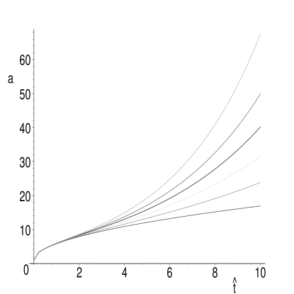
Figure 1: The scale factor $a(\hat{t})$ with $q(0)=0$. The curves from bottom to top have $\xi$ increasing from $0$ to ${1\over 6}^{-}$.

The first three graphs show the effect of increasing $\xi$ while keeping $q(0)$ fixed. The effect on the scale factor is to introduce acceleration at late time. This effect is independent of the Vaidya radiation and is also found in the non-radiating case lamasym2 ; both1 . (See lamasym2 ; lamasym1 ; perk for asymmetry in bulk cosmological constants, bhasym for asymmetry in (constant) bulk black hole masses, and both1 ; both2 for both types of asymmetry). The effects of the radiating brane occur predominantly at early times.

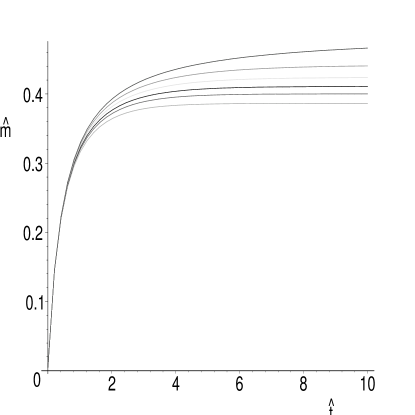
Figure 2: The average black hole mass function $\hat{m}(\hat{t})$ with $q(0)=0$. The curves from top to bottom have $\xi$ increasing from $0$ to ${1\over 6}^{-}$.

There is also a marked effect on the average mass function $\hat{m}$. The increase of $\hat{H}$ when $\xi$ is increased in Eq. (35) leads to a decrease in $\hat{m}^{\prime}$ by Eq. (32), which results in a suppression of the asymptotic value of $\hat{m}$. Since the asymptotic value determines the dark radiation at nucleosnthesis (where $\rho\ll\lambda$), this suppression of $\hat{m}$ means that nucleosynthesis limits LSR can be more easily satisfied when there is asymmetry.

Figure 3 shows that even if there is no initial difference in the black hole mass functions on either side of the brane, and given that the radiation from the brane is symmetric, a difference in the mass functions will still develop during the evolution, because of the different curvatures on either side of the brane.

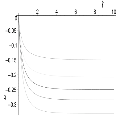
Figure 3: The difference in black hole masses, $q(\hat{t})$, with parameters as in Fig. 2

Figures 4 and 5 demonstrate the effect of varying $q(0)$ for a fixed $\xi$. Although there is little discernible difference in the scale factor for the different values of $q(0)$, the increase in $\hat{H}$ for larger $q(0)$ is still enough to suppress the final value of $\hat{m}$. (The shape of the $q$ curve is the same as in Fig. 3 for all the initial values.)

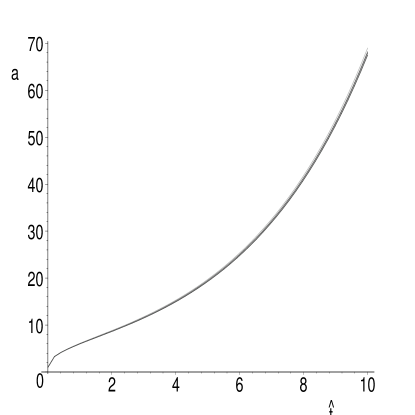
Figure 4: The scale factor $a(\hat{t})$ with $\xi={1\over 6}^{-}$ and $q(0)=0$, $10$, $20$, $30$, $50$ and $100$, from bottom to top curve. Variation in $q(0)$ has little effect on the evolution of $a$.

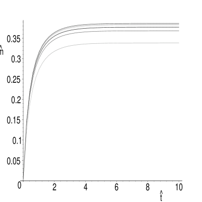
Figure 5: The average black hole mass function $\hat{m}(\hat{t})$ with $\xi=0$ and (curves from top to bottom) $q(0)=0$, $10$, $20$, $30$ , $50$ and $100$.

If we assume that the asymmetry is small, i.e. $q/a^{4}$ and $\xi$ are small, then we can perturb away from the symmetric solution, Eqs. (23)–(25), and evaluate the early- and late-time solutions. At early times,

$${q\over a^{4}}\approx\frac{3\alpha}{4+\alpha}\left(1+{t_{2}\over t}\right)\,,$$ (36)

where $t_{2}$ is a constant of integration which must be of a suitable size to keep the whole expression within our smallness assumptions. This type of decay at early times is confirmed in Fig. 3. At late times,

$${q}\approx Be^{-C/t^{2}}\,,$$ (37)

where $B,C$ are constants. The asymptotic value, $q\to B$, is evident in Fig. 3.

IV Conclusion

We have derived the dynamical equations for a radiating brane in a Vaidya-AdS bulk, without assuming $Z_{2}$ symmetry. The radiation from the brane propagates in different curvature regions on either side, given the difference in bulk cosmological constants and initial black hole masses on either side. There are four cases, depending on whether the radiation falls into a black hole or escapes to infinity on either side of the brane.

We performed numerical integrations of the equations in the case where radiation feeds black holes on both sides of the brane. One of the key features that emerges is the suppression of the late-time dark radiation (the asymptotic value of the average mass parameter) due to asymmetry.

These solutions correspond to the case $\epsilon_{\pm}=1$ in Eq. (9), or $\overline{\epsilon}=+1,\Delta\epsilon=0$ in Eq. (18). The other three cases have radiation escaping to infinity on at least one side of the brane, but in these cases, the total brane energy density $\rho+\lambda$ is negative or can change sign. Further investigation is needed to determine whether any of these cases admit physically reasonable models.

Acknowledgments:

LÁG was supported by OTKA grants Nos. T046939, TS044665 and by a PPARC visitor grant, EL by an EPSRC DTA grant, and RM by PPARC.

References

- (1) See, e.g., P. Brax and C. van de Bruck, Class. Quantum Grav. 20, R201 (2003) [arXiv:hep-th/0303095]; R. Maartens, Liv. Rev. Rel. 7 (2004) [arXiv:gr-qc/0312059].
- (2) A. Hebecker and J. March-Russell, Nucl. Phys. B608, 375 (2001) [arXiv:hep-ph/0103214]; E. Kiritsis, N. Tetradis, and T. N. Tomaras, JHEP 03, 019 (2002) [arXiv:hep-th/0202037].
- (3) D. Langlois, L. Sorbo, and M. Rodríguez-Martínez, Phys. Rev. Lett. 89, 171301 (2002). The conversion to the notation of this paper is
- (4) D. Langlois and L. Sorbo, Phys. Rev. D68, 084006 (2003) [arXiv:hep-th/0306281].
- (5) A. Chamblin, A. Karch, and A. Nayeri, Phys. Lett. B509, 163 (2001) [arXiv:hep-th/0007060].
- (6) E. Leeper, R. Maartens, and C. Sopuerta, Class. Quant. Grav. 21, 1125 (2004) [arXiv:gr-qc/0309080].
- (7) M. Minamitsuji and M. Sasaki, Phys. Rev. D70, 044021 (2004) [arXiv:gr-qc/0312109].
- (8) R. A. Battye, B. Carter, A. Mennim, and J. P. Uzan, Phys. Rev. D64, 124007 (2001) [arXiv:hep-th/0105091]; G. Huey and J. Lidsey, Phys. Rev. D66, 043514 (2002) [arXiv:astro-ph/0205236]; A. Padilla, arXiv:hep-th/0406157.
- (9) B. Carter and J. P. Uzan, Nucl. Phys. B606, 45 (2001) [arXiv:gr-qc/0101010].
- (10) N. Deruelle and T. Dolezel, Phys. Rev. D62, 103502 (2000) [arXiv:gr-qc/0004021].
- (11) W. B. Perkins, Phys. Lett. B504, 28 (2001) [arXiv:gr-qc/0010053].
- (12) P. Kraus, JHEP 12, 011 (1999) [arXiv:hep-th/9910149]; D. Ida, JHEP 09, 014 (2000) [arXiv:gr-qc/9912002]; A. C. Davis, I. Vernon, S. C. Davis, and W. B. Perkins, Phys. Lett. B504, 254 (2001) [arXiv:hep-ph/0008132].
- (13) H. Stoica, S.-H. Henry Tye, and I. Wasserman, Phys. Lett. B482, 205 (2000) [arXiv:hep-th/0004126]; P. Bowcock, C. Charmousis, and R. Gregory, Class. Quant. Grav. 17, 4745 (2000) [arXiv:hep-th/0007177].
- (14) L.Á. Gergely, Phys. Rev. D68, 124011 (2003) [arXiv:gr-qc/0308072]. The conversion to the notation of this paper is
- (15) This generalizes Eq. (21) in lamasym1 , which covers non-radiating models.