Numerical computation of constant mean curvature surfaces using finite elements

Abstract

This paper presents a method for computing two-dimensional constant mean curvature surfaces. The method in question uses the variational aspect of the problem to implement an efficient algorithm. In principle it is a flow like method in that it is linked to the gradient flow for the area functional, which gives reliable convergence properties. In the background a preconditioned conjugate gradient method works, that gives the speed of a direct elliptic multigrid method.

1 Introduction

The computation of surfaces with prescribed mean curvature is an important problem in numerical relativity with an abundance of applications. We will only give a few examples here, which we had in mind while developping this algorithm.

The first example are marginally trapped surfaces, that is closed spherical surfaces $\Sigma$ in a Riemannian 3-manifold $(M,g)$, such that $H\pm P=0$ on $\Sigma$. Here $H$ denotes the mean curvature of $\Sigma$ and $P=\textrm{tr}_{\Sigma}K$ is the trace of $K$ along $\Sigma$. The extra tensor field $K$ on $M$ represents the second fundamental form of $M$ in spacetime. Apparent horizons are outermost marginally trapped surfaces and are used in numerical simulations for various purposes like black hole location or excision of black holes in numerical simulations inside their apparent horizon. For an introduction and furter references see for example [1, 2].

In the special, time symmetric case $K=0$, i.e. $P=0$, these surfaces are minimal surfaces, that is critical points of the area functional. When surfaces of minimal area are considered that satisfy the additional constraint, that they include a given volume with the minimal surface, the minimal surface can be “blown up” to render an evenly spaced, geometrically defined foliation of the exterior domain, as it is explained in Huisken and Yau [3] and Huisken [4]. The surfaces of this foliation have constant mean curvature

$$H=\textrm{const}\,.$$

This the Euler-Lagrange equation to the constrained problem. It is a quasilinear, second order, degenerate elliptic equation for the position of the surface. The size of the enclosed volume, as well as the area of the constant mean curvature surfaces is then a generic candidate for a geometric radial coordinate.

Besides this, there are more applications for constant mean curvature foliations. One of them is to define a concept for the center of mass of an isolated gravitating system [3]. Another application is that a geometrically defined foliation also can be used to construct geometric gauge conditions for time evolution in the Einstein equations as described in [5]. In addition the proof of the Riemannian Penrose inequality by Bray [6] uses isoperimetric surfaces, which are special cases of constant mean curvature surfaces. This proof establishes the monotonicity of the Hawking mass on these surfaces with increasing enclosed volume, given a positive energy condition. This energy condition translates into the geometric condition for $M$ to have nonnegative scalar curvature. The numerically computed constant mean curvature surfaces may therfore be used to detect and measure gravitational fields.

A considerable number of methods have been exploited to find apparent horizons, a current overview of which is given in Thornburg [7]. Baumgarte and Shapiro [2] also review some techniques for locating apparent horizons. Schnetter [8] computed the more general “constant expansion surfaces” with $H\pm P=\textrm{const}$. These methods can be classified into three different approaches, namely flow like methods using a curvature flow to locate the apparent horizon, direct methods using a Newton method to solve the elliptic apparent horizon equation, and indirect minimization methods that try to minimize an $L^{2}$-error integral.

The flow like methods are very robust as they converge for a large set of initial data and are able to model the change of topology by using level set methods [9, 10]. However, these methods are rather slow. The more and more popular direct elliptic methods are very fast but have a small domain of convergence as is noted by Thornburg [7]. The minimization methods are problematic, since minimizing the $L^{2}$-error functional corresponds to solving a fourth order PDE, while the actual problem is only a second order PDE. This does not only spoil the condition of the problem, but may also introduce invalid solutions. All these methods, however, share the fact that they use finite differencing.

In contrary, this article describes a finite element based direct minimization method to compute constant mean curvature surfaces

$$H=\textrm{const}\,,$$

that inherits it the big domain of convergence from the flow like method, while rivaling the speed of the direct elliptic method. The method as it is presented here can not be applied without modification to horizon finding in the general non-time symmetric case with $K\not\equiv 0$, but an appropriate modification is outlined in section 3.6.

We consider $\mathbf{R}^{3}$ to be equipped with a general metric $g_{ij}$. For the purposes of general relativity this metric will be asymptotically flat, that is in rectangular coordinates the metric components satisfy

$$g_{ij}=\delta_{ij}+\mathcal{O}(r^{-1})\,.$$

We also will consider two-dimensional spherical surfaces $\Sigma\subset\mathbf{R}^{3}$. The induced metric on $\Sigma$ will be denoted by $\gamma$, the outer normal by $\nu$ and the second fundamental form $A=\nabla\nu$. The mean curvature is labeled $H=\textrm{tr}_{\Sigma}A$. In the following we use Einstein’s summation convention such that Latin indices range from 1 to 3 whereas Greek indices range from 1 to 2. We will frequently use the abbreviation CMC for “constant mean curvature”.

Section 2 will explain the relationship of constant mean curvature surfaces to the isoperimetric problem and give some theoretical results concerning existence and properties of constant mean curvature surfaces. The algorithm is explained in section 3 and some numerical examples are given in section 4.

2 Theoretical Background

This paper uses the fact that constant mean curvature surfaces are critical points of the isoperimetric problem. The isoperimetric problem is to find a surface enclosing a given volume that has minimal area. Formulated precisely, this is

Definition 2.1

Let $M$ be a Riemannian manifold, then a compact subset $\Omega\subset M$ is called a solution to the isoperimetric problem if for all $\Omega^{\prime}\subset M$ with $\textrm{Vol}\,(\Omega^{\prime})=\textrm{Vol}\,(\Omega)$ the inequality

$$|\partial\Omega|\leq|\partial\Omega^{\prime}|$$

holds.

To treat this problem with tools from the calculus of variations one denotes by a variation in $M$ a smooth map $F:M\times(-\varepsilon,\varepsilon)\rightarrow M$ such that $F(\cdot,0):M\rightarrow M$ is the identity and for all $t\in(-\varepsilon,\varepsilon)$ the map $F(\cdot,t):M\rightarrow M$ is a diffeomorphism. We collect the following facts from the literature, see eg. [11] for a flat background metric or [12] in the general case.

Lemma 2.2

Given any set $\Omega\subset M$ with smooth boundary $\Sigma=\partial\Omega$ and a variation $F$ with normal velocity $f=g\left(\left.\frac{\partial F}{\partial t}\right|_{t=0},\nu\right)$ on $\Sigma$, the following variation formulas for the volume $\textrm{Vol}\,(\cdot)$ of $\Omega$ and area $|\cdot|$ of $\Sigma$ hold.

$$\left.\frac{\rmd}{\rmd t}\right|_{t=0}\textrm{Vol}\,(F(\Omega,t)) = \int_{\Sigma}f\,\rmd\mu_{\Sigma}$$

$$\left.\frac{\rmd}{\rmd t}\right|_{t=0}|F(\Sigma,t)| = \int_{\Sigma}Hf\,\rmd\mu_{\Sigma}$$

Therefore $H$ can be interpreted as $L^{2}$-gradient of the area functional, and the constant function $1$ as the $L^{2}$-gradient of the volume functional. We have the following characterization of volume preserving variations.

Lemma 2.3

If $F$ is a variation that preserves the volume of $\Omega\subset M$, then $\int_{\Sigma}fd\mu_{\Sigma}=0$ for $\Sigma=\partial\Omega$ and $f$ the normal velocity of $F$ on $\Sigma$. Conversely, if $f$ is a function with $\int_{\Sigma}fd\mu_{\Sigma}=0$ then there exists a volume preserving variation with $f$ as normal velocity.

Introducing the usual Lagrangian, the Euler-Lagrange equation of the isoperimetric problem can be computed.

Proposition 2.4

If $\Omega$ is a smooth solution to the isoperimetric problem, then $\Omega$ is bounded by a constant mean curvature surface.

This only characterizes critical points of the isoperimetric problem. To give a better description the usual concept of stability has to be introduced.

Definition 2.5

A constant mean curvature surface is called stable if the second variation of area in volume preserving directions is nonnegative, and strictly stable if it is positive.

Due to the characterization of volume preserving variations in lemma 2.3, a sufficient condition for stability is the nonnegativity of the Jacobi operator

$$Jf=-\Delta f-f\left(|A|^{2}+\textrm{Ric}(\nu,\nu)\right)$$

that is the inequality

$$\int_{\Sigma}f^{2}\left(|A|^{2}+\textrm{Ric}(\nu,\nu)\right)\,\rmd\mu\leq\int_{\Sigma}|df|^{2}\,\rmd\mu$$

for all $f\in C^{\infty}(\Sigma)$ with $\int f=0$. A constant mean curvature surface $\Sigma$ is strictly stable, if there exist $\alpha>0$ such that

$$\alpha\int_{\Sigma}f^{2}\,\rmd\mu\leq\int_{\Sigma}fJf\,\rmd\mu$$

for all $f$ with $\int f=0$. A strictly stable constant mean curvature surface is an isolated local minimum of the isoperimetric problem, in the sense that there is no volume preserving variation that does not increase area.

The algorithm presented was constructed having in mind spatial slices of isolated gravitating systems in general relativity. These slices have (in absence of linear momentum) the following asymptotic behavior of the metric.

Definition 2.6

A strongly asymptotically flat manifold is a Riemannian manifold $M$ together with a metric $g$, such that there is a compact set $C\subset M$ and a diffeomorphism $x:M\setminus C\rightarrow\mathbf{R}^{3}\setminus B_{R}(0)$ for some $R$ and, such that, in the coordinates given by $x$, the metric $g$ has the form

$$g_{ij}=\left(1+\frac{m}{2r}\right)^{4}\delta_{ij}+Q_{ij}$$

with the following decay conditions

$$|Q_{ij}|\leq Cr^{-2}\quad|\partial^{l}Q_{ij}|\leq Cr^{-2-l}\quad l=1,2,3,4$$

In this setting Huisken and Yau [3] have proved the following

Theorem 2.7

Let $(M,g)$ be a strongly asymptotically flat manifold with $m>0$. Then there exists a compact set $C\subset M$ such that on $M\setminus C$ exists a unique foliation by spherical constant mean curvature surfaces, such that

1. for growing radius these surfaces approximate Euclidean spheres,

2. the centers of these spheres converge to a point in $\mathbf{R}^{3}$,

3. and the respective surfaces are strictly stable with respect to the isoperimetric problem.

For the purposes of this article, the way Huisken and Yau establish the existence of constant mean curvature surfaces is very interesting. They use the volume preserving mean curvature flow. Solving this flow means finding a map $F:\Sigma_{0}\times(0,T)\rightarrow N$ for an initial surface $\Sigma_{0}\subset M$ with

$$\frac{\partial F}{\partial t} = (h-H)\nu\qquad\textrm{for}\qquad t\geq 0$$

$$F(0) = \Sigma_{0}$$

where $h=|\Sigma_{t}|^{-1}\int_{\Sigma_{t}}Hd\mu_{t}$ with $\Sigma_{t}=F(\Sigma_{0},t)$. Huisken and Yau show that in the above setting a solution exists for all times, in case the flow is started from a Euclidean sphere of radius bigger than some critical radius. For $t\rightarrow\infty$ the surfaces $\Sigma_{t}$ then converge to a surface with constant mean curvature.

In view of the variational perspective, this is the flow to the gradient of the area functional projected onto the volume preserving variations, which is a technique for solving constrained minimization problems. Huisken and Yau show that this method converges. The key issue in this proof is the stability of the CMC-surfaces. That is, these surfaces are local minimizers of the isoperimetric problem.

These facts enable us to use a constrained minimization algorithm to approach the numerical computation of constant mean curvature surfaces, since the most efficient of these methods rely on the positivity of the second variation.

3 Description of the Algorithm

As explained before, Huisken and Yau [3] have shown that a projected gradient flow method for constrained minimization converges in the analytic case. From the numerical viewpoint there are much better methods for solving such problems, since projected gradient methods tend to converge slowly and do not preserve the constraint during iteration.

The approach taken here is to convert the constrained problem into an unconstrained minimization problem, which is then solved by a preconditioned conjugate gradient method.

3.1 The surface model

Discrete surfaces are modeled as a triangulated meshes, that is sets of vertices, edges and triangles linked together according to the topology of the triangulation.

To each vertex $p$ of a given triangulation $\tilde{\mathcal{T}}$ a variation vector $r(p)$ is attached. A vertex can only move into this direction. Associated to $\tilde{\mathcal{T}}$ is a discrete set of linear finite elements

$$\mathcal{S}=\left\{\sum_{p\in\mathcal{T}}\alpha_{p}\phi_{p}:\alpha_{p}\in\mathbf{R}\right\}$$

where $\phi_{p}(q)=\delta_{pq}$ for all vertices $q$ of the triangulation and $\phi_{p}$ restricted to a triangle is linear. As indicated in the definition, the functions $\phi_{p}$ form a basis of $\mathcal{S}$, called the nodal basis. A function $u\in\mathcal{S}$ is therefore characterized by its values in the vertices of the triangulation.

Given any $u\in\mathcal{S}$ the graph of $u$ over $\tilde{\mathcal{T}}$ is the triangulation $\mathcal{T}$ with the vertices $p=\tilde{p}+u(\tilde{p})r(\tilde{p})$. Fix a reference triangulation $\tilde{\mathcal{T}}$ and model the unknown surface as graph of a finite element function over $\tilde{\mathcal{T}}$.

For the purposes of applying hierarchical basis preconditioning, the implementation uses a hierarchical data structure described by Leinen [13]. This object oriented approach stores the triangles in a tree, the roots being coarse triangles with their subtriangles as child nodes whenever the coarse triangle is divided. The edges form a similar structure. To link edges and triangles, these two trees have cross references according to their topology, such as triangles consisting of edges and edges being part of triangles.

An excellent outline of the method of finite elements and issues of numerical integration as needed in the next section is given in [14].

3.2 Discrete Area and Volume Functionals

To compute the area of a triangulation it is clearly possible to compute the area of each triangle and sum up. The computation of the area of a single triangle takes place in a standard situation. Define the standard triangle $T_{S}\subset\mathbf{R}^{2}$ as the set

$$T_{S}=\left\{(x_{1},x_{2})\in\mathbf{R}^{2}:x_{1},x_{2}\geq 0,x_{1}+x_{2}\leq 1\right\}$$

Every triangle $T=\Delta(p_{0},p_{1},p_{2})\subset\mathbf{R}^{3}$ of the triangulation is diffeomorphic to $T_{S}$ via the linear map

$$F_{T}:T_{S}\rightarrow T:(x_{1},x_{2})\mapsto(1-x_{1}-x_{2})p_{0}+x_{1}p_{1}+x_{2}p_{2}\,.$$

Then the area of $T$ is given by

$$A(T)=\int_{T_{S}}\sqrt{\det(\gamma_{\alpha\beta})}\rmd x$$ (1)

where $\gamma_{\alpha\beta}$ are the components of the induced metric on $T$ in the coordinates induced by $F_{T}$. If $\mathbf{R}^{3}$ was equipped with the Euclidean metric, $\sqrt{\det(\gamma_{\alpha\beta})}$ would be a constant on $T$. Then a quadrature formula to integrate (1) exactly is given by

$$A(T)=\frac{1}{2}\sqrt{\det\left(\gamma_{\alpha\beta}(1/3,1/3)\right)}$$

and this is the integration rule used to define the discrete area

$$\hat{A}(T)=\frac{1}{2}\sqrt{\det\left(\gamma_{\alpha\beta}(1/3,1/3)\right)}\,.$$ (2)

For this integration rule we obtain that

$$|A(T)-\hat{A}(T)|\leq c_{0}h^{2}A(T)\,,$$

where $h$ is the (Euclidean) diameter of $T$ and $c_{0}=c_{0}(g,\partial g,\partial^{2}g)$ depends on the metric $g$, in particular, we have the bounds $c_{0}\leq Cr^{3}$ in view of definition 2.6. The above formula gives that for the whole triangulation we have

$$|A(\mathcal{T})-\hat{A}(\mathcal{T})|\leq c_{0}h_{\textrm{max}}^{2}A(\mathcal{T})$$

where $h_{\textrm{max}}$ is the maximal diameter of the triangles of $\mathcal{T}$.

The discrete area $\hat{A}$ is as differentiable with respect to the values of $u_{p}$ as the background metric $g$. Explicit formulas for the derivatives of $\hat{A}$ can be computed. These formulas contain first derivatives of $g$ in the $r(p)$ directions.

Consider for example the triangle $T_{0}$ with vertices $(p_{0},p_{1},p_{2})$ and move $p_{1}$ into the $r(p_{1})=r_{1}$-direction, which gives a family of triangles $T_{\varepsilon}=\Delta(p_{0},p_{1}+\varepsilon r_{1},p_{2})$. Then look at the following map

$$F_{\varepsilon}:T_{S}\rightarrow T_{\varepsilon}:(x_{1},x_{2})\rightarrow(1-x_{1}-x_{2})p_{0}+x_{1}(p_{1}+\varepsilon r(p_{1}))+x_{2}p_{2}$$

and compute the $\varepsilon$-derivative of the discrete area expression in (2) using these coordinates. This gives

$$\left.\frac{\rmd}{\rmd\varepsilon}\right|_{\varepsilon=0}\hat{A}(T_{\varepsilon}) = \frac{1}{4\hat{A}(T_{0})}\left(\gamma_{22}\,g(X_{1},r_{1})-\gamma_{12}\,g(X_{2},r_{1})\right)$$

$$+\frac{1}{24\hat{A}(T_{0})}\left(\gamma_{11}\Lambda_{22,1}+\gamma_{22}\Lambda_{11,1}+2\gamma_{12}\Lambda_{12,1}\right)\,.$$

Here $X_{\alpha}=p_{\alpha}-p_{0}$, $\gamma_{\alpha\beta}=\gamma_{\alpha\beta}(1/3,1/3)$ and

$$\Lambda_{\alpha\beta,\delta}=\left.\frac{\partial g_{ij}}{\partial y^{k}}\right|_{F_{0}(1/3,1/3)}r^{k}_{\delta}X^{i}_{\alpha}X^{j}_{\beta}\,.$$

Similar formulas can be derived for all vertices.

To define the discrete volume functional, a fixed reference triangulation $\tilde{\mathcal{T}}$ and a function $u$ is required. The discrete volume functional is defined as the oriented discrete volume enclosed by the shell between $\tilde{\mathcal{T}}$ and the graph of $u$ over $\tilde{\mathcal{T}}$. Orientation is chosen such that positive $u$ gives positive volume and negative $u$ negative volume, that is the $r(p)$ are interpreted to point outward.

For the computation of the volume corresponding to a single triangle, define the standard prism $P_{S}=T_{S}\times[0,1]$. The prism $P_{S}$ can be mapped to the volume $P$ between a triangle $\tilde{T}$ of $\tilde{\mathcal{T}}$ with vertices $\tilde{p}_{0},\tilde{p}_{1},\tilde{p}_{2}$ and the corresponding triangle $T$ of $\textrm{graph}u$ with vertices $p_{i}=\tilde{p}_{i}+u(\tilde{p}_{i})r(\tilde{p}_{i})$, $i=0,1,2$ via

$$G_{P}:P_{S} \rightarrow P$$

$$(x_{1},x_{2},x_{3}) \mapsto \left(1-x_{3}\right)\left(\left(1-x_{1}-x_{2}\right)\tilde{p}_{0}+x_{1}\tilde{p}_{1}+x2\tilde{p}_{2}\right)$$

$$+x_{3}\left(\left(1-x_{1}-x_{2}\right)p_{0}+x_{1}p_{1}+x_{2}p_{2}\right)$$

as illustrated in figure 1 .

Figure 1: Standard prism mapped to volume corresponding to one triangle.

The oriented volume of $P$ is then given by

$$\int_{P}1\,\textrm{dvol} = \int_{P}\sqrt{\det(g_{ij})}\,\rmd x$$

$$= \int_{P_{S}}\sqrt{\det(g_{ij}\circ G_{P})}\det(d_{x}G_{P})\,\rmd x\,.$$

We choose the sign of this expression to match the orientation condition given above. The integral in this formula is again replaced by a quadrature formula which is exact in the case of a Euclidean background metric. Such a formula can be constructed as product of a quadrature formula for $T_{S}$ and one for $[0,1]$. For $T_{S}$ we can use the center of gravity rule previously used for the area. For $[0,1]$ an integration rule which is exact for polynomials of degree two is sufficient. Such a rule is for example given by the two-point Gauss rule with weights $1/2$ and evaluation points $1/2\pm 1/\sqrt{12}$ which is exact for polynomials of degree three. The formula for discrete volume computed with a general integration rule for $[0,1]$ with the $N$ weights $a_{k}$ and evaluation points $z_{k}$ then reads

$$\hat{V}(P)=\sum_{k=1}^{N}a_{k}\sqrt{\det(g_{ij}\left(G_{P}(1/3,1/3,z_{k})\right)}\det(\rmd_{x}G_{P})(1/3,1/3,z_{k})$$ (3)

There is no problem to evaluate these terms, but more elegantly $\det(\rmd_{x}G_{P})(1/3,1/3,x_{3})$ can be written as a polynomial in $u_{p}$ of degree up to three. The six non-zero coefficients of this polynomial can be computed from $\tilde{\mathcal{T}}$ only. Therefore evaluation of this term only requires the evaluation of this polynomial.

For this functional the error bounds

$$|V(T)-\hat{V}(T)|\leq c_{1}h^{2}U|V(T)|\,$$

hold, with analogous bounds for the volume of the whole triangulation. Here $h$ is the maximum of the diameters of $T$ and $\tilde{T}$, $U=\max\{|u(p_{i})r(p_{i})|:i=0,1,2\}$ and $c_{1}=c_{1}(g,\partial g,\partial^{2}g)$ depends on the metric with $c_{1}\leq Cr^{-3}$ in view of definition 2.6.

The discrete volume functional is again as differentiable with respect to the nodal values of $u$ as the metric $g$. Explicit formulas for these derivatives can be computed from (3) in the same way as for the area functional.

The discrete volume and area functionals are therefore constructed to give the right answer in the Euclidean case since the asymptotically flat situation suggests that this gives a good guess. Indeed, the error bounds given above improve rapidly for growing radius. Their values and derivatives can be computed per triangle using a fixed procedure, that is fixed time. Thus evaluation of these two functionals takes time proportional to the number of triangles.

Evaluation of the functionals and their derivatives requires the evaluation of the metric and its derivatives at the requested points. Therefore, if the metric is given on a grid it is necessary to interpolate these values.

Note that the gradient of the area functional is a discrete, weak analogon to the mean curvature. This can be seen from lemma 2.2 and the fact that deforming $\textrm{graph}u$ over a triangulation by increasing $u_{p}$ at one point $p$ corresponds to a variation of $\textrm{graph}u$ with variation vector field $\phi_{p}r_{p}$.

3.3 Optimization techniques

Now we have a problem of the following form:

minimize $$\hat{A}(u)\quad u\in\mathcal{S}\approx\mathbf{R}^{N}$$

s.t. $$\hat{V}(u)-V_{0}=0$$

with $\hat{A}(u)$ the area of $\textrm{graph}u$ over a fixed reference triangulation and $\hat{V}(u)$ the discrete oriented volume between $\textrm{graph}u$ and the reference triangulation as described above.

Naturally one would consider a Lagrange method, that is computing the critical points of the Lagrangian function

$$L:\mathcal{S}\times\mathbf{R}\rightarrow\mathbf{R}:(u,\lambda)\mapsto\hat{A}(u)-\lambda\left(\hat{V}(u)-V_{0}\right)\,.$$

However, since a local minimum of (3.3) does not correspond to a minimum of $L$ but merely to a critical point of $L$, minimization methods are not applicable. Thus solving the critical point equation directly with a Newton method is the only alternative in view, but this is not desirable, since it would involve second derivatives of the metric $g$.

For numerical optimization however, there is a better method, namely the augmented Lagrangian method. This considers the following penalized Lagrangian function

$$L_{\rho}(u,\lambda)=\hat{A}(u)-\lambda\left(\hat{V}(u)-V_{0}\right)+\frac{\rho}{2}\left(\hat{V}(u)-V_{0}\right)^{2}$$

with a penalty parameter $\rho$. The following theorem can be proved using standard calculus methods on the submanifold generated by the constraint. However, a more elementary proof can be found in [15, Theorem 12.2.1].

Theorem 3.1

If $\hat{A}$ and $\hat{V}$ are $C^{2}$, $u^{*}$ is a solution to (3.3), $\lambda^{*}$ is the exact value of the Lagrange parameter, and the Hessian of $\hat{A}$ at $u^{*}$ is positive in directions perpendicular to $\textrm{grad}V$, then $u^{*}$ is a critical point of $L_{\rho}(\cdot,\lambda^{*})$ and there exists $\rho_{0}$ such that for all $\rho>\rho_{0}$ the Hessian of $L_{\rho}(\cdot,\lambda^{*})$ is positive definite, that is, $u^{*}$ is a strict local minimum of $L_{\rho}(\cdot,\lambda^{*})$.

Note that in the analytic case, theorem 2.7 implies that the conditions of this theorem hold. A CMC-surface is therefore a local minimum for the analytic penalized Lagrangian for suitable penalty and Lagrange parameters. For the discrete case we can still assert the regularity assumption, but we unfortunately do not know about stability.

To solve (3.3) we minimize the augmented Lagrangian. To find the Lagrange parameter to the desired volume the following algorithm is used:

• $\rho\leftarrow\textrm{some value}>\rho_{0}$

• $\lambda_{0}\leftarrow\textrm{good initial guess}$

• $k\leftarrow 0$

• repeat

  • Minimize $L_{\rho}(\cdot,\lambda_{k})$ to get approximative solution $u_{k}$

  • $\lambda_{k+1}\leftarrow\lambda_{k}-\rho\left(\hat{V}(u_{k})-V_{0}\right)$

  • $k\leftarrow k+1$

• until $|\lambda-\lambda^{*}|<\varepsilon$

If the conditions of theorem 3.1 hold, then this algorithm converges locally in $(\lambda_{k})$ to $\lambda^{*}$ and then the $(u_{k})$ converge to $u^{*}$. Convergence improves for $\rho\rightarrow\infty$. For a proof of this fact cf. [16].

A “good initial guess” for $\lambda$ can be obtained from the Euclidean situation. If a surface is considered that has a radius of approximately $r$ then $2/r$, the Euclidean mean curvature of a sphere of radius $r$, is a good choice, but in practice, starting with $\lambda=0$ also works well.

Each pair $(u_{k},\lambda_{k})$ obtained by one step of the above algorithm corresponds to a discrete CMC-surface and its discrete mean curvature, of course not with $V(u_{k})=V_{0}$, but rather $V(u_{k})=V(u_{k})$. This explains why not many steps have to be performed when one just wants to find CMC-surfaces together with their mean curvature and area, but not necessarily a particular enclosed volume.

The parameter $\rho$ should neither be chosen too small nor too big, since a value too small gives that the minimization method diverges and a value too big gives a bad condition of the minimization problem. An estimate for $\rho_{0}$ can be obtained by estimates for the Jacobi operator from Huisken-Yau [3]. These estimates indicate that $\rho_{0}$ decays like $r^{-3}$, where $r$ is the radius of the surface considered. But the condition of the problem is not affected if $\rho$ is chosen to decay like $r^{-2}$ since that is the scaling of the other terms of the Hessian matrix of $L_{\rho}$, which controls the condition of the problem. Therefore the exact choice of $\rho$ is not very critical, but decreasing $\rho$ should be attempted.

The penalized Lagrangian method is used to transform the constrained problem into an unconstrained minimization. The method we chose to numerically solve this is the conjugate gradient method. Although the conditions of theorem 3.1 imply local convergence of such a method, the rate of convergence depends on the basis chosen for $\mathcal{S}$. The nodal basis is not a very good choice, since the number of steps to make increases proportionally to the number of points of the triangulation and would therefore give an algorithm with quadratic time complexity.

The similarity of the problem to the solution of linear elliptic PDEs suggests that one try methods from this field that have proven to give good convergence rates. The choice made here is to use hierarchical bases that give the CG method multigrid like speed while being very simple to implement. Using this preconditioner, an overall time complexity of $\mathcal{O}(N\log N)$ for linear problems is achieved with $N$ being the number of vertices of the triangulation. Section 4.5 describes some examples and shows that the speedup is significant, and reduces complexity even in the nonlinear case.

Optimization methods are presented in Fletcher [17, 15]. For details on hierarchical bases see Bank, Dupont and Yserentant [18] and Yserentant [19, 20].

3.4 Computation of single surfaces

When a single surface has to be computed we can take the full advantages of the hierarchical finite element representation, and use a cascading technique for iteration as proposed by Bornemann and Deuflhard [21]. We start with a given coarse triangulation and iterate to get a first coarse approximation to the surface. Then we refine this triangulation by dividing each triangle into four new triangles. The surface obtained from the coarse grid iteration then can be used as initial value to the fine grid iteration. This procedure can be continued until the desired resolution is reached. This cascading technique gives an immense speedup.

3.5 Computation of foliations

When the method is used to compute whole families of constant mean curvature surfaces close to Euclidean spheres it is possible to use the previously computed surface as initial data for the next iteration. To do that, one has to produce a sequence of appropriate reference surfaces and volume conditions that give a reasonable sequence of surfaces.

The following is suggested in a situation when one knows one discrete constant mean curvature surface $\mathcal{T}$ that is centered. In this case, the radial direction on this surface can be used as the variation direction of the vertices.

To produce a new surface at distance $r$ further out (in), $\mathcal{T}$ should be replaced by the graph of the constant function $r$ ($-r$) over $\mathcal{T}$. This graph then will be the new reference surface $\tilde{\mathcal{T}}$.

The constrained minimization problem to consider now is to minimize $\hat{A}$ while keeping $\hat{V}=0$. This leads to an algorithm where not much volume is inbetween the reference surface and the unknown constant mean curvature surface, which is desirable since this increases the accuracy of the discrete volume functional.

The problem of finding the first constant mean curvature surface can sometimes be solved by simply minimizing area without the constraint. This will give a discrete minimal surface, which can serve as starting surface. However, not all manifolds have a single spherical minimal surface that can be used.

Another method to get a starting surface is to start with a Euclidean sphere of big radius, use its normal direction as variation direction and solve the constrained problem. However, if a significant translation occurs, the solver should be restarted using a coordinate sphere around the computed center as initial surface, since the distortion in the triangulation reduces the resolution, for illustration see figure 2. Alternatively one could use adaptive mesh refinement here.

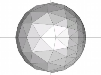
Figure 2: A translated triangulation has reduced resolution. This is the final iterate of an area minimization in Schwarzschild, started from a translated sphere.

3.6 Generalizing the Algorithm

The algorithm described above is based on the variational structure of the equation

$$H=\textrm{const}\,.$$

In view of numerical relativity it would be very interesting to find surfaces $\Sigma$ that solve the equations

$$H\pm P=\textrm{const}$$ (4)

with $P=\tr_{\Sigma}K=\tr_{M}K-K(\nu,\nu)$, $\nu$ the unit normal to $\Sigma$, and $(M,g,K)$ are an initial data set for the Einstein equations.

However these equations are not the Euler-Lagrange equations for any functional considering surfaces in $M$. This is due to the fact that the term $P$ depends on the normal of the surface in consideration. In contrary the equation

$$H+H_{0}=\textrm{const}$$

where $H_{0}:M\to\mathbf{R}$ does not depend on the normal of the surface is the Euler-Lagrange equation for a constrained minimization problem, in the sense that it is satisfied on the boundary $\partial\Omega$ of a set $\Omega\subset M$ minimizing

$$J(\Omega)=|\partial\Omega|+\int_{\Omega}H_{0}\,\rmd\mu\qquad\Omega\subset M$$

subject to $$\int_{\Omega}\,\rmd\mu=V_{0}\equiv\textrm{const}\,.$$

For a given initial surface $\Sigma_{0}$ with normal vector field $\nu_{0}$ we may therefore fix a function $P_{0}=\tr K-K(\nu_{0},\nu_{0})$ and extend it to a neighborhood of the initial surface by the condition that it does not change along the radial directions considered in 3.1. Then we solve the equation $H\pm P_{0}=\textrm{const}$ using the procedure described before. An iteration of this strategy will produce a sequence of surfaces and normals that might converge. If they converge, then the limit is a solution of the discrete version of equation 4.

The author currently works on implementing, testing and examining this approach, but came to the conclusion that this preliminary outline for extending this algorithm might be interesting for applications in numerical relativity.

4 Numerical Examples

In this section we present three examples based on metrics of the Brill-Lindquist-Type. This is a conformally flat metric on $\mathbf{R}^{3}$ of the form

$$g_{ij}(x)=\left(1+\sum_{k=1}^{N}\frac{m_{k}}{|x-x_{k}|}\right)\delta_{ij}$$

This metric represents a spacelike slice containing $N$ Schwarzschild-Type singularities at the points $x_{k}$ of mass $m_{k}$. The metric and its derivatives were evaluated analytically at every requested point.

The triangulations used for the computations in this section are based on the octahedron, that is the triangulation with vertices $\pm e_{i}$, $i=1,2,3$, and regular refinement of it. To regularly refine a triangulation, every triangle is divided into four subtriangles by introducing the midpoint of its edges as new vertices to the triangulation. If these new points are projected to the sphere one obtains the surfaces shown in figure 3. Rescaled and translated versions of these triangulations in different refinement states will serve as starting surfaces.

All pictures of surfaces shown in this section were created using geomview [22].

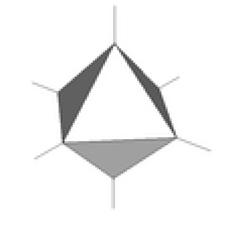
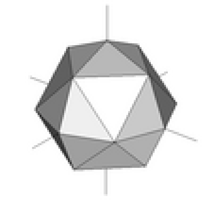
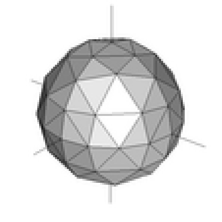
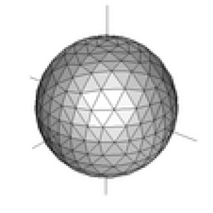
Figure 3: Several refinement states of the octahedron.

4.1 Schwarzschild Solutions

Here $N=1$, $m_{1}=1$ and $x_{1}=0$. This case was included to test the convergence of the method. To compare the numerical results with the analytically known results, introduce the following radius function for a surface $\Sigma$

$$\tilde{r}=|\Sigma|^{-1}\int_{\Sigma}|x|d\mu_{\Sigma}$$

where $|\cdot|$ denotes Euclidean distance to the origin. Using the center of gravity rule for numeric integration, this radius can be computed approximately, which gives for each triangulation $\mathcal{T}$ a discrete radius $\hat{r}(\mathcal{T})$.

Starting the method with the minimal surface and computing outward, one obtains a family of triangulations $\mathcal{T}_{k}$, and a family of Lagrange parameters $\lambda_{k}$ which can be interpreted as the constant mean curvature of these triangulations. The exact mean curvature of a sphere of radius $r$ in the spatial Schwarzschild metric is plotted as continuous line in figure 5 whereas the Lagrange parameters versus the numerical radius of each triangulation is plotted as mark. This data results from a resolution 6 triangulation.

Since a good approximation to the mean curvature is known, the Hawking mass on constant mean curvature surfaces

$$m_{H}(\Sigma)=\frac{|\Sigma|^{1/2}}{(16\pi)^{3/2}}\left(16\pi-|\Sigma|H^{2}\right)$$

can easily be computed. Figure 5 shows the absolute value of the difference of the Hawking mass of each surface and the expected value 1. The initial surfaces were not centered here but translated by $d=0,0.1,0.2,0.3,0.4$, resolution is again 6.

Figure 4: Exact and computed mean curvature compared for different radius.

Figure 5: The difference of the Hawking mass for different translated initial spheres and the expected value 1.

To test the ability of finding the center, the method was started with Euclidean spheres of radius 20 and center $(d,0,0)$ for different values of $d$. Then a CMC surface of equal volume was computed using the value 0.0005 as penalty parameter. The Euclidean distance of the center of this surface to the origin is shown in table 1 for different resolutions and different values of $d$. The resolution number is the number of refinement steps applied to each triangle. Resolution 3,4,5,6,7 correspond to 258,1026,4098,16386,65538 vertices. This table shows nearly the expected second order convergence, which corresponds to a factor of 4.

Table 1: Distance of the computed center to the origin for translated starting surfaces of radius 20 off center by distance $d$ and the associated convergence factor $f$ for $d=5$.

• Resolution	$d=1$	$d=2$	$d=3$	$d=4$	$d=5$	$f$	$d=5$
  4	0.01791	0.03521	0.05394	0.07245	0.09161	4/5	3.93
  5	0.00455	0.00903	0.01382	0.01869	0.02329	5/6	3.95
  6	0.00112	0.00230	0.00343	0.00472	0.00589	6/7	3.98
  7	0.00030	0.00060	0.00086	0.00115	0.00148

A direct elliptic method fails to converge when started with a very rough surface near the horizon, as is reported by Thornburg [7]. To test this aspect of our method, we construct rough data by starting with a sphere of radius 1/4 and refining up to level 5. The vertices that are created by the last refinement step are moved outward to a radius of 3/4 such that the starting surface oscillates around the minimal surface. In comparison to spheres of radius 1/4 and 3/4 as starting surfaces, the iteration takes significantly longer, about three times, but still converges. The diagnostic quantity $E:=\max_{\textrm{all vertices}}|r-0.5|$ is plotted in figure 6 for spheres of radius 1/4 and 3/4 and the rough surface as initial surface. The iteration stopped, when the relative change in $E$ was less than 1/1000.

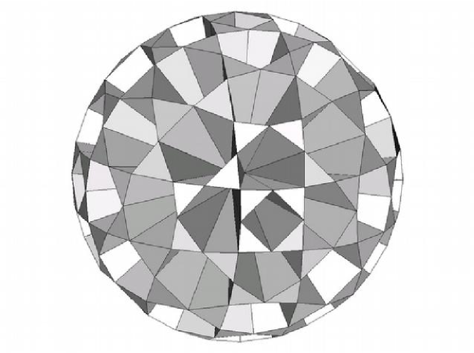
Figure 6: A rough initial surface on the left and the the maximum of the absolute deviation of $r$ from 1/2 during an iteration for this surface. For comparison the data for an iteration with smooth data is shown.

4.2 Two singularities

Here we examine a metric with $N=2$, $m_{k}=1$ and $x_{k}=\pm de_{1}$. This space contains two minimal surfaces, each one enclosing one of the singularities.

The first test was to find the critical value $d^{*}$, such that the two singularities are enclosed by common a minimal surface for $d<d^{*}$ but not for $d>d^{*}$. Refinement up to level 7 indicates that $|d^{*}-0.766362|\leq 0.000002$, which deviates by $0.02\%$ from the value $0.76619745$ reported by Thornburg in [23]. The area of this minimal surface is computed as $196.41579$, whereas Thornburg reported a value of $196.407951$ which deviates by $0.004\%$. We noticed however, that with increasing resolution the value of $d^{*}$ and the area of the minimal surface decreased with our procedure, therefore for larger resolution the values reported here might become closer to the values of Thornburg.

For $d>d^{*}$, computation cannot start at a minimal surface, since this does not exist. That is why for this problem the algorithm is started from a Euclidean sphere with big radius centered at 0. In each step the radius has been reduced approximately by $1/10$. In figure 9 every tenth surface for $d=5$ is drawn. The two small surfaces are the minimal surfaces enclosing the singularities.

It is clear that for growing radius, the Hawking mass of the surfaces approaches the ADM-mass, which in this case is the total mass of the two singularities, namely 2. The difference of of the Hawking mass and the expected value is plotted in figure 8 for $d=1,2,3,4,5$.

The computed area, mean curvature and Hawking mass for $d=1$ of a surface with approximate radius $5$ for different resolutions and the associated convergence factor is shown in table 2.

Figure 8 shows the mean quadratic deviation of the Euclidean radius function from the expected radius. This figure shows that the surfaces become rounder with growing radius as predicted by the theory.

Figure 7: The error the Hawking mass for two singularities of mass 1.

Figure 8: The mean quadratic deviation of the radius function for two singularities of mass 1.

Table 2: Area, mean curvature $H$, Hawking mass $m$ and associated convergence factors for the surfaces computed form a coordinate sphere with radius 5 in the $d=1$-metric for two singularities.

• Resolution	Area	$H$	$m$		$f_{\textrm{Area}}$	$f_{\textrm{H}}$	$f_{\textrm{m}}$
  3	646.68121	0.1860585	1.9893651	$\frac{3-4}{4-5}$	3.97	3.88	3.80
  4	649.42623	0.1857211	1.9926138
  5	650.11737	0.1856342	1.9934694	$\frac{4-5}{5-6}$	4.00	3.97	3.95
  6	650.29032	0.1856123	1.9936860

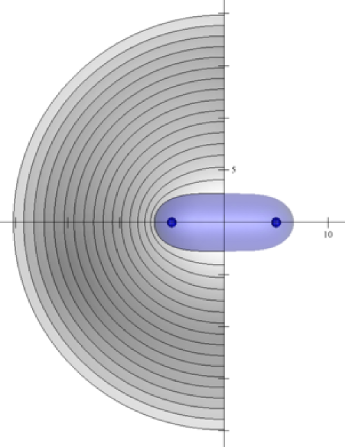
Figure 9: The foliation for two singularities of mass 1 and distance 5 to the origin. The innermost surface is the last surface computed by the method, for smaller surfaces the algorithm seems to fail converging.

4.3 Three singularities

Here we study a very symmetric Brill-Lindquist metric with three singularities at $x_{1}=0$, $x_{2/3}=\pm e_{1}$ and masses $m_{1}=2$, $m_{2}=m_{3}=2\sqrt{2}$. This comes from the stereographic projection of a metric conformal to the standard metric on $S^{3}\subset\mathbf{R}^{4}$. The conformal factor on the sphere is the sum of the Greens functions to the conformal Laplacian at the points $\pm(1,0,0,0)$ and $\pm(0,0,0,1)$, rescaled such that in the standard stereographic projection of $S^{3}\setminus(0,0,0,1)$, the resulting metric has the Brill-Lindquist form.

An analogous picture is shown in figure 10, where it is clarified that for each asymptotically flat end an outermost minimal surface exists. Additionally there are two minimal surfaces resulting from the mirror symmetry along the planes, that divide the picture in equal halves. As it turns out, these additional minimal surfaces are stable and can be found by minimization.

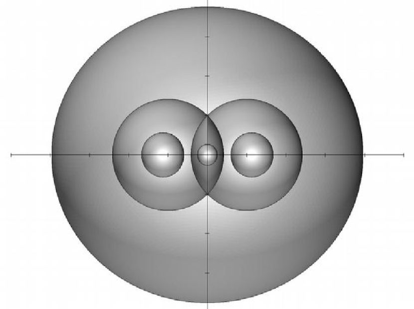
Figure 10: $S^{3}$ with four points blown to infinity by conformal rescaling, illustrated by $S^{2}$ on the left and in the stereographic projection with minimal surfaces on the right.

The intersection of these minimal surfaces with the $x^{1}x^{2}$-plane is drawn in figure 10 in the stereographic projection. The smaller surfaces enclosing one singularity and the big surface enclosing all three singularities correspond to the outermost minimal surfaces of the asymptotically flat ends. The surfaces enclosing two singularities correspond to the surfaces arising from the symmetry. The area of the outermost minimal surfaces is given in figure 3. The surface named (R)ight encloses the singularity at $(1,0,0)$, the surface called (M)iddle encloses the singularity at the origin, and the surface called (O)uter encloses all three singularities. These areas should be the same due to symmetry. Therefore we compute the convergence factors of the differences to zero and obtain, as also shown in figure 3, perfect second order convergence.

Table 3: The area of two different minimal surfaces and the convergence of its difference.

• Resolution	R	M	O	f	R-M	R-O
  3	2966.95	2970.59	2970.84	3/4	4.10	4.09
  4	2951.64	2952.53	2952.59	4/5	4.02	4.02
  5	2947.79	2948.01	2948.03	5/6	4.00	4.00
  6	2946.83	2946.88	2946.89	6/7	4.00	4.00
  7	2946.59	2946.60	2946.60

This symmetry enables us to compute these surfaces exactly. In $\mathbf{R}^{4}$ the surfaces are the intersections of $S^{3}$ with the planes $y^{1}=\pm y^{4}$ and project to the surfaces given by the quadratic equation

$$Q(x):=|x|^{2}\pm 2x^{1}-1=0$$

In figure 11 we plot $\max_{\textrm{all vertices}}|Q(x)|$ for an iteration started on a sphere with radius 1 centered at $(0.5,0,0)$ for different resolutions. We again find quadratic convergence for increasing resolution.

Figure 11: The maximum value of $|Q(x)|$ for iterations in different resolutions.

4.4 Kerr Solutions

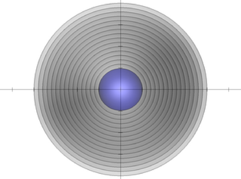
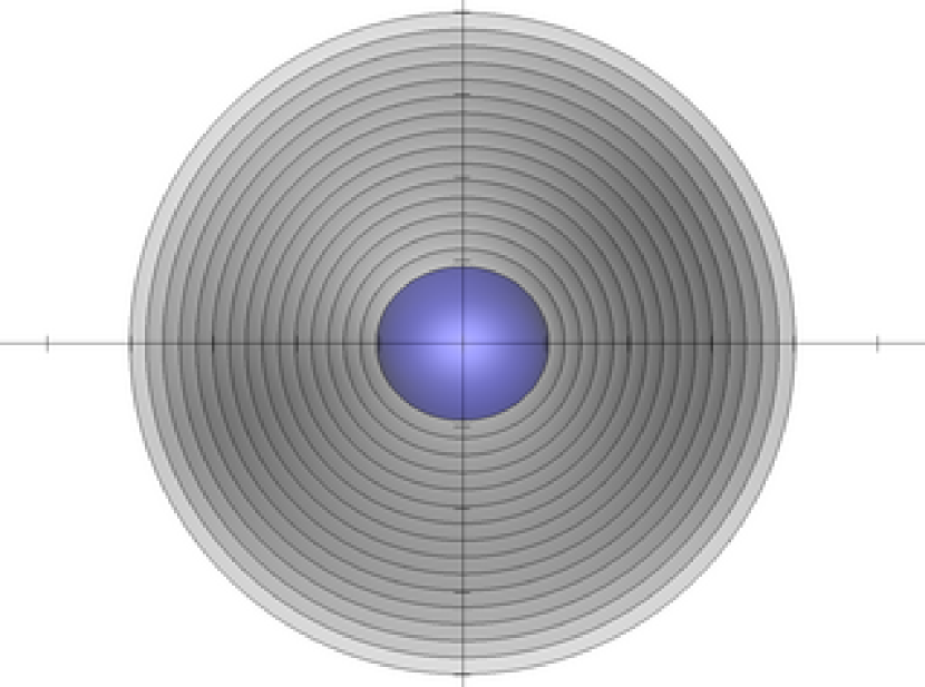
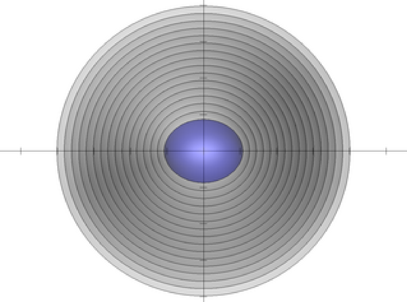
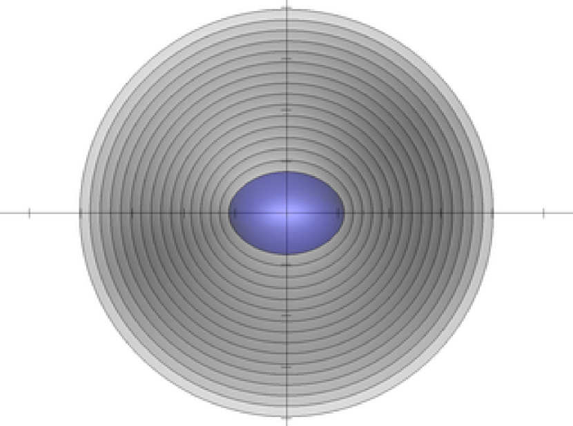
Figure 12: The intersection of the constant mean curvature surfaces with the $x_{1}x_{2}$-plane in Kerr for $a=0.3$, $a=0.5$, $a=0.7$ and $a=0.9$. The ticks on the axes are in unit distance, the area radii of the innermost surfaces are 13.28, 14.38, 15.75 and 17.11, further surfaces could not be computed.

For this test, a $\{t=\textrm{const}\}$-slice of the Kerr metric in Kerr-Schild coordinates is used. The associated 3-metric is given by

$$g_{ij}=\delta_{ij}+2Hl_{i}l_{j}$$

with

$$H=\frac{MR}{R^{2}+a^{2}\cos^{2}\theta}\qquad l_{i}=\left(\frac{Rx^{1}+ax^{2}}{R^{2}+a^{2}},\frac{Rx^{2}-ax^{1}}{R^{2}+a^{2}},\frac{x^{3}}{R}\right)$$

where

$$R^{2}=\frac{1}{2}(r^{2}-a^{2})+\sqrt{\frac{1}{4}(r^{2}-a^{2})^{2}+a^{2}(x^{3})^{2}}\qquad\cos^{2}\theta=\frac{(x^{3})^{2}}{R^{2}}$$

and $r^{2}=|x|^{2}$ is the Euclidean distance. This metric has an apparent horizon at $\{R=R_{+}\}$, $R_{+}=M+\sqrt{M^{2}-a^{2}}$ if $a<1$. Unfortunately in this slicing the horizon is not a CMC-surface in contrast to the Boyer-Lindquist $\{t=\textrm{const}\}$ slices, and cannot be found with the method presented here.

We therefore start again at a large radius $r=20$ with a centered sphere and compute inwards reducing the radius by 0.1 in each step. Some of the inner surfaces for different values of $a$ are shown in figure 12. The last surface shown is the last surface computed by the method. The mean curvature of some more surfaces is plotted for these values of $a$ in figure 13, while the mean quadratic deviation of the radius function from constant radius and the hawking mass is shown in figure 14 for the same values of $a$. This figure displays the remarkable fact that the hawking mass of the CMC-surfaces is nearly independent of $a$, while not constant. The same shape of the graph even holds for $a=0$, where the CMC-surfaces are perfectly round coordinate spheres. Figures 13 and 14 show the data of 190 surfaces that are nearly equidistant with distance 0.1, while in figure 12 only 15 of the innermost surfaces with distance 0.2 are shown. The apparent horizon is shown in none of these pictures, since it is not a CMC-surface. In the above plots we use the geometric area radius $r_{g}=\sqrt{|\Sigma|/4\pi}$ on the horizontal axes.

Figure 13: The mean curvature of the CMC-surfaces in Kerr for $a=0.3,0.5,0.7$ and $0.9$.

Figure 14: Left, the mean quadratic deviation of the radius function of its mean value, right the hawking mass, of the CMC-surfaces in Kerr spacetime for $a=0.3,0.5,0.7$ and $0.9$.

4.5 Performance

This section reviews the performance of the algorithm. All times reported here have been measured on a personal computer with a single Athlon XP 2000+ CPU. The first performance test is intended for comparing this method to others. The metric used is the unit mass Schwarzschild metric $g_{S}=(1+\frac{1}{2r})^{4}\delta$. The aim was to find the horizon, so area minimization without volume constraint was attempted. The initial surface is taken as discrete sphere of radius 1 with center $(0.3,0,0)$. We use a low resolution of 3 to start and initially optimize. Then we refine to the next resolution, take the surface obtained from the coarse grid iteration as initial values for the fine grid optimization, and iterate this process until the desired resolution is obtained.

Since the horizon is a Euclidean sphere of radius $1/2$ we use $E:=\max_{\textrm{all vertices}}|r-1/2|$ as diagnostic parameter. Iteration is stopped when $E$’s relative change is less than $1/1000$ for more than four iterations. Table 4 shows the iterations elapsed for each refinement level and the total time elapsed up to reaching the result, including the coarse grid iterations. Note that the final values for $E$ display nearly perfect second order convergence. Figure 15 shows the value of $E$ for each iteration of the algorithm with maximal refinement level 8 starting with refinement level 3. The levels of the cascade correspond to the convergent regime of the algorithm for the current refinement level, while the edges occur when refinement has been done.

Table 4: Elapsed Time and Iterations for the Schwarzschild test.

• Resolution	Number	Iterations	Total	final value
  	of points	on finest Level	Time [s]	of E
  3	258	25	0.44	0.014472349
  4	1025	22	3.22	0.003732145
  5	4098	26	16	0.000945821
  6	16386	21	58	0.000236132
  7	65538	39	374	0.000060190
  8	262146	42	1726	0.000015141

Figure 15: The maximum of the absolute value of the radius function minus 0.5 monitored during the iteration of a three to eight refinement steps run.

To test the speedup of the hierarchical basis transformation, we go back to Brill-Lindquist data with two singularities and $d=1$. We start with a large coordinate sphere of radius $10$, translated by $1$ and test the time used to center this sphere to a constant mean curvature surface using the nodal and hierarchical basis. We again used the cascading technique with initial refinement level 3. As diagnostic parameter we use the the $l^{2}$-gradient norm times two to the power of the number of refinement levels, which is nearly independent of the refinement level. The stopping condition was to reduce this value by a factor of 2000. We chose to do only one minimization and therefore started with the previously computed Lagrange parameter $\lambda=0.13531$. The total time elapsed and the number of iterations in the highest resolution is plotted in figure 16. We see a substantial improvement in the number of iterations involved and the elapsed time.

Figure 16: Total time (left) and the number of iterations for the highest refinement level (right) plotted versus the number of refinement levels.

4.6 Comparison to other methods

Comparison of the speed of this method to other methods available is very difficult at this stage. This is mainly due to the following three issues. At first there are no standardized tests nor standardized platforms on which to test nor agreements with what accuracy to stop, which are general problems. Second, the figures presented by Schnetter [8] and Thornburg [23] do not refer to the computation of CMC-Surfaces but to the computation of apparent horizons, which is a different equation in general and especially in the cases considered by them. And third, as stated before, our method uses an explicit evaluation of the metric, whereas Schnetter and Thornburg use interpolation of the metric from a given grid discretizing the metric on the ambient three-manifold. As evaluation of the metric takes more than half of the execution time in our case, it is hard to judge whether we compare the underlying algorithms or just the different methods of evaluating the metric.

However, in table 5 we display some figures taken from Thornburg to show in comparison to table 4 at least that the execution time of our algorithm is in the same order of magnitude as the times given by Thornburg. Thornburg tries to find the horizon in a boosted slice of Kerr data with angular momentum $a=0.8$ and velocity $v=0.8$. The numbers refer to execution time on a dual Intel Pentium IV 1.7 GHz which executes his algorithm on one processor, where in contrast we worked on a single AMD Athlon XP 2000+.

Table 5: Values reported by Thornburg for horizon finding in a boosted Kerr time slice, with different resolutions.

• Number of points	Total Time[s]
  533	2.0
  1121	4.2
  2945	13
  7905	43
  25025	220

5 Conclusion

We have presented an algorithm to compute constant mean curvature surfaces based on a finite element discretization. The implementation displays convergence, accuracy and speed rivaling the methods based on finite differencing used in production runs. But still the implementation by the author is academic in the sense that not much effort has been spent on optimization and fitting the code into standard environments such as Cactus for example.

However, creating a fully functional apparent horizon finder based on finite element discretization, i.e. the extention of this algorithm to not necessarily time symmetric initial data, is still a long way to go, but the author’s opinion is that the results presented here are very encouraging.

References

References

- [1] Dreyer O, Krishnan B, Shoemaker D and Schnetter E 2003 Phys. Rev. D 67 024018
- [2] Baumgarte T W and Shapiro S L 2003 Phys. Rep. 376 p 41–131
- [3] Huisken G and Yau S T 1996 Invent. Math. 124 p 281–311
- [4] Huisken G 1998 Trends in Mathematical Physics (Knoxville, TN, 1998) (Providence: American Mathematical Society) p 299–306
- [5] Krivan W and Herold H 1995 Class. Quant. Grav. 12 p 2297–2308
- [6] Bray H L 1997 Ph.D. Dissertation Stanford University
- [7] Thornburg J 1996 Phys. Rev. D 54 p 4899–4918
- [8] Schnetter E 2003 Class. Quant. Grav. 20 p 4719–4737
- [9] Tod K P 1991 Class. Quant. Grav. 8 p L115–L118
- [10] Shoemaker D, Huq M F and Matzner R A 2000 Phys. Rev. D 62 124005
- [11] Barbosa J L and do Carmo M 1984 Math. Z. 185 p 339–353
- [12] Barbosa J L and do Carmo M 1988 Math. Z. 197 p 123–138
- [13] Leinen P 1995 Computing 55 p 325–354
- [14] Ciarlet P G and Lions J-L, eds. 1991 Handbook of numerical analysis. Vol II. Finite element methods. Part 1. (Amsterdam: North-Holland)
- [15] Fletcher R 1981 Practical Methods of Optimization, Vol. 2 (Chicester, New York, Brisbane, Toronto: John Wiley & Sons)
- [16] Powell M J D 1969 in Fletcher R, ed. Optimization (Academic Press, London and New York) p 283–298
- [17] Fletcher R 1980 Practical Methods of Optimization, Vol. 1 (Chicester, New York, Brisbane, Toronto: John Wiley & Sons)
- [18] Bank R E, Dupont T and Yserentant H 1988 Numer. Math. 52 p 427–458
- [19] Yserentant H 1986 Numer. Math. 49 p 379–412
- [20] Yserentant H 1992 ICIAM (Washington 1991) (Philadelphia: SIAM) p 256–276
- [21] Bornemann F A and Deuflhard P 1996 Numer. Math. 75(2) p 135–152
- [22] Phillips M et al. 2000 Geomview Manual (The Geometry Center – http://www.geomview.org)
- [23] Thornburg J 2004 Class. Quant. Grav. 21(2) p 743–766