The Hough transform search for continuous gravitational waves

Abstract

This paper describes an incoherent method to search for continuous gravitational waves based on the Hough transform, a well known technique used for detecting patterns in digital images. We apply the Hough transform to detect patterns in the time-frequency plane of the data produced by an earth-based gravitational wave detector. Two different flavors of searches will be considered, depending on the type of input to the Hough transform: either Fourier transforms of the detector data or the output of a coherent matched-filtering type search. We present the technical details for implementing the Hough transform algorithm for both kinds of searches, their statistical properties, and their sensitivities.

I Introduction

Rapidly rotating neutron stars are expected to be the primary sources of continuous gravitational waves, and the current generation of earth-based gravitational wave detectors might be able to detect them. Recent analysis of data from the first science runs of the LIGO S1:detector ; ligo1 ; ligo2 and GEO S1:detector ; GEO1 ; GEO2 interferometric detectors has already led to upper limits on the gravitational waves emitted by the pulsar J1939+2134 and its equatorial ellipticity S1:pulsar . The analysis of future science runs is expected to lead to upper limits below other astrophysical constraints, and eventually to detections.

The analyses presented in S1:pulsar were based on the coherent integration of the detectors’ output for the entire observation time (approximately 17 days) and used a Bayesian time-domain method and a frequentist frequency-domain jks approach. The searches were not computationally expensive, targeting a single known pulsar and processing only a narrow frequency band of about 0.5 Hz around the pulsar emission frequency for a fixed sky location and spin-down rate known from radio observations.

Future continuous wave searches will involve searching longer data stretches (of order weeks to months) for unknown sources over a large frequency band, vast portions of the sky and spin-down parameter values. It is well known that the computational cost of coherent techniques for searches of this type is absolutely prohibitive bccs . Thus hierarchical methods have been proposed.

In hierarchical strategies incoherent techniques (less sensitive and less computationally expensive) are used to scan the data and the parameter space for interesting candidates which are then followed up with coherent searches. Different strategies can be envisaged that combine the data incoherently. All methods use, in some way, the power from the Fourier transforms of short stretches of data: in the frequency bins where the signal is present there should systematically be an excess of power. In order to compensate for the frequency modulation imposed on the signal by the Earth’s motion and the pulsar’s spin-down during the observation period, one must use not the power from the same frequency bins in each successive Fourier transform, but rather from the bins where one expects the signal peak to be.

In the so called stack-slide method, one “slides” the frequency bins of each Fourier transform to line-up the signal peaks and then simply sums the power bc . The Hough transform method can be seen as a variation on this where, after the sliding, one sums not the power but just zeros and ones, depending on whether the power in the frequency bin exceeds a threshold or meets some other criterion. Whereas in low signal-to-noise conditions in Gaussian noise, the standard power summing method is possibly optimal, the Hough transform method might be more robust in the presence of large spectral disturbances. To see this, consider the case when a large spectral disturbance is present only in a single Fourier transform. This could have a very large effect on the power sum statistic, but no matter how large, this spectral line could only add $+1$ to the Hough statistic.

The Hough transform is a robust parameter estimator of multi-dimensional patterns in images and it finds many applications in astronomical data analysis storkey ; ballester ; ca . In the context of image processing, it provides robustness against missing data points or discontinuous features ik . It was initially developed by Paul Hough to analyze bubble chamber pictures at CERN, and later patented by IBM hough1 ; hough2 . It is currently being used to analyze data from the LIGO and GEO detectors. The codes employed for these analyses are freely available as part of the LIGO Algorithms Library lal . The VIRGO project virgo ; virgo97 is also setting up a similar hierarchical search pipeline. Studies of hierarchical strategies can be found in fp ; sp ; pss ; bfpr ; afp ; f .

This paper is organized as follows: section II briefly describes the expected waveforms from an isolated spinning neutron star and summarizes the general strategy of a hierarchical search. Section III presents the general idea of the Hough transform and section IV describes its implementation for non-demodulated input data, and section V studies its statistical properties. Section VI describes the Hough search using demodulated input data and finally section VII summarizes our main results.

II Preliminaries

II.1 The signal from a pulsar

In this subsection we fix our notation and briefly review the expected gravitational wave signal from a spinning neutron star. Further details about the pulsar signal can be found in jks ; a concise review of the possible physical mechanisms that may be causing pulsars to emit gravitational waves can be found in S1:pulsar . For our purposes, we only need the form of the gravitational wave signal as seen by an Earth based detector.

Let $\mathbf{n}_{1}$ and $\mathbf{n}_{2}$ denote the unit vectors pointing along the arms of the detector and denote by $\zeta$ the angle between the arms. Let $\mathbf{z}$ be the unit vector parallel to $\mathbf{n}_{1}\times\mathbf{n}_{2}$. Apart from the detector frame $(\mathbf{n}_{1},\mathbf{n}_{2},\mathbf{z})$, we also have the wave frame $(\mathbf{x}_{w},\mathbf{y}_{w},\mathbf{z}_{w})$ in which the unit vector $\mathbf{z}_{w}$ is along the direction of propagation of the wave and $(\mathbf{x}_{w},\mathbf{y}_{w},\mathbf{z}_{w})$ form a right-handed orthonormal system. Finally, $\mathbf{n}=-\mathbf{z}_{w}$ is the unit vector pointing in the direction of the neutron star; see figure 1.

Figure 1: The detector frame and the wave frame.

The spacetime metric $g_{\mu\nu}$ can be written as a perturbation of the flat metric $\eta_{\mu\nu}$: $g_{\mu\nu}=\eta_{\mu\nu}+h_{\mu\nu}$. The received gravitational wave $h_{\mu\nu}$ has the form

$$h_{\mu\nu}(t)=h_{+}(t)\left(\mathbf{e}_{+}\right)_{\,\mu\nu}+h_{\times}(t)\left(\mathbf{e}_{\times}\right)_{\,\mu\nu}$$ (1)

where $\mathbf{e}_{+}=\mathbf{x}_{w}\otimes\mathbf{x}_{w}-\mathbf{y}_{w}\otimes\mathbf{y}_{w}$ and $\mathbf{e}_{\times}=\mathbf{x}_{w}\otimes\mathbf{y}_{w}+\mathbf{y}_{w}\otimes\mathbf{x}_{w}$, and $t$ denotes clock time at the location of the (moving, accelerating) detector, which we refer to as detector time. The waveforms for the two polarizations are

$$h_{+}(t)=A_{+}\cos\Phi(t)\,,\qquad h_{\times}(t)=A_{\times}\sin\Phi(t)$$ (2)

where $\Phi(t)$ is the phase of the gravitational wave and $A_{+,\times}$ are the amplitudes; $A_{+,\times}$ are constant in time and depend on the other pulsar parameters such as its rotational frequency, moments of inertia, the orientation of its rotation axis, its distance from Earth etc. The phase $\Phi(t)$ takes its simplest form when the time coordinate used is $t_{\textrm{\mbox{\tiny{NS}}}}$, the proper time in the rest frame of the neutron star:

$$\Phi_{\textrm{\mbox{\tiny{NS}}}}(t_{\textrm{\mbox{\tiny{NS}}}})=\phi_{0}+2\pi\sum_{n=0}^{s}\frac{f_{(n)}^{(\textrm{\mbox{\tiny{NS}}})}}{(n+1)!}t_{\textrm{\mbox{\tiny{NS}}}}^{n+1}$$ (3)

where $\phi_{0}$, $f_{(0)}^{(\textrm{\mbox{\tiny{NS}}})}$ and $f_{(n)}^{(\textrm{\mbox{\tiny{NS}}})}$ ($n\geq 1$) are respectively the phase, instantaneous frequency and the spin-down parameters in the rest frame of the star at the fiducial start time $t_{\textrm{\mbox{\tiny{NS}}}}=0$, and $s$ is the number of spin-down parameters included in our search.

We refer the reader to jks for the expression of $\Phi(t)$ in the detector frame as a function of detector time. For our purposes, we only need to know that the instantaneous frequency $f(t)$ of the wave as observed by the detector is given, to a very good approximation, by the familiar non-relativistic Doppler formula:

$$f(t)-\hat{f}(t)=\hat{f}(t)\frac{{\bf v}(t)\cdot\bf{n}}{c}$$ (4)

where $\mathbf{v}(t)$ is the detector velocity in the Solar System Barycenter (SSB) frame and $\hat{f}$ is given by

$$\hat{f}(t)=f_{(0)}+\sum_{n=1}^{s}\frac{f_{(n)}}{n!}\left(t-t_{0}+\frac{\Delta\mathbf{r}(t)\cdot\mathbf{n}}{c}\right)^{n}$$ (5)

where $t_{0}$ is the fiducial detector time at the start of the observation, the $f_{(n)}$ are the spin-down parameters as measured in the SSB frame (these need not be equal to the $f_{(n)}^{(\textrm{\mbox{\tiny{NS}}})}$; see jks ), and $\Delta\mathbf{r}(t):=\mathbf{r}(t)-\mathbf{r}(t_{0})$ with $\mathbf{r}(t)$ being the position of the detector in the SSB frame at time $t$. We have also assumed the neutron star to be moving with uniform speed relative to the Sun and is so far away that there are no observable proper-motion effects. (These could be taken into account if necessary, at the cost of introducing further parameters.)

The detector output is a linear combination of $h_{+}$ and $h_{\times}$:

$$h(t)=F_{+}(\mathbf{n},\psi)\,h_{+}(t)+F_{\times}(\mathbf{n},\psi)\,h_{\times}(t)$$ (6)

where $F_{+,\times}$ are known as the the antenna pattern functions of the detector and depend on the direction $\mathbf{n}$ to the star and also on the polarization angle $\psi$ which determines the orientation of the $(\mathbf{x}_{w},\mathbf{y}_{w})$ axes in their plane. In addition, the antenna pattern functions also depend on the detector parameters such as its latitude, the angle $\zeta$ between its arms, and the azimuth of the bisector of the arms. Due to the motion of the Earth, $F_{+,\times}(\mathbf{n},\psi)$ depend implicitly on time and for notational convenience, we shall usually denote the antenna pattern functions as $F_{+,\times}(t)$. Thus, the received signal is both amplitude- and frequency-modulated.

The search method described in this paper depends on finding a signal whose frequency evolution fits the pattern produced by the Doppler shift and the spin-down. The parameters which determine this pattern are the ones which appear in equation (4), namely, $(f_{(0)},\{f_{(n)}\},{\mathbf{n}})$; these parameters will be collectively denoted by $\vec{\xi}$.

The amplitudes $A_{+,\times}$ are determined by the other pulsar parameters such as the orientation of its axis, its ellipticity, its distance from Earth etc. The search method presented in this paper depends only on the phase model of equation (3). The exact form of the amplitudes is model dependent. As an illustrative example, consider the wave emitted by a deformed spinning neutron star as in S1:pulsar . If $f_{r}$ is the rotational frequency of the star, the frequency of the gravitational wave is $2f_{r}$. The additional parameters determining this component of the pulsar signal are $\iota$ and $h_{0}$ where $\iota$ is the angle between the pulsar’s axis of rotation and the vector $\mathbf{z}_{w}=-\mathbf{n}$, and $h_{0}$ characterizes the amplitude of the emitted gravitational wave. The amplitudes $A_{+,\times}$ are:

$$A_{+} = \frac{1}{2}h_{0}(1+\cos^{2}\iota)\,,$$ (7)

$$A_{\times} = h_{0}\cos\iota\,.$$ (8)

If we assume the emission mechanism is due to deviations of the pulsar’s shape from perfect axial symmetry, then the amplitude $h_{0}$ will be

$$h_{0}=\frac{16\pi^{2}G}{c^{4}}\frac{I_{zz}\epsilon f_{r}^{2}}{d}$$ (9)

where $d$ is the distance of the star from Earth, $I_{zz}$ is the z-z component of the star’s moment of inertia with the $z$-axis being its spin axis, and $\epsilon:=(I_{xx}-I_{yy})/I_{zz}$ is the equatorial ellipticity of the star. Among all the quantities appearing in this equation, the value of $\epsilon$ is by far the most uncertain. Typical values are expected to be $\sim 10^{-8}$ for standard neutron stars and values of $\sim 10^{-6}$ are expected to be the maximum values bccs . There is also a very small uncertainty in the value of $f_{r}$ because the pulsar could have a (presently unobservable) radial velocity. This would produce a Doppler shift between the true value of $f_{r}$ in the neutron star (NS) frame, and its measured value on Earth. Assuming typical values of the radial velocity to be the same as the typically measured transverse velocities ($\sim 500$ km/s, see e. g. ktr ), we get an uncertainty in $f_{r}$ of $\sim 0.1$%.

II.2 A multi-stage hierarchical search

Consider performing a blind search for pulsars using a bank of templates and relying only on coherent matched filter techniques. Since a larger observation time implies better resolution in the space of frequency, spin-downs and sky-positions, the number of templates increases rapidly as a function of the total observation time. A typical example is an all-sky search for young, fast pulsars, i.e. for hypothetical signals with frequency $\hat{f}<f_{\textrm{\mbox{\tiny{max}}}}=1000$Hz and spin-down ages greater than $\tau>\tau_{\textrm{\mbox{\tiny{min}}}}=40$yr. Let $s$ be the number of spin-down parameters that we search over and let $T_{\textrm{\mbox{\tiny{obs}}}}$ be the total observation time. The number of templates required for this search has been calculated in equation (6.3) of bccs :

$$N_{p}\approx{\textrm{max}}_{s\in\{0,1\ldots\}}[N_{s}F_{s}(T_{\textrm{\mbox{\tiny{obs}}}})]$$ (10)

where

$$N_{s}=\left(\frac{f_{\textrm{\mbox{\tiny{max}}}}}{1\textrm{kHz}}\right)^{s+2}\left(\frac{40\textrm{yr}}{\tau_{\textrm{\mbox{\tiny{min}}}}}\right)^{s(s+1)/2}$$ (11)

gives the spin-down scaling and $F_{s}$ is a function that depends on the observation time; for large observation times, $F_{s}\propto T_{\textrm{\mbox{\tiny{obs}}}}^{5}$. We have taken the maximum allowed fractional mismatch in observed signal power between the signal and the template to be 0.3. For example, if $s=2$, assuming the observation time is significantly longer than a day, equation (6.7) of bccs approximates to :

$$F_{2}(T_{\textrm{\mbox{\tiny{obs}}}})\approx 2.2\times 10^{7}\times\left(\frac{T_{\textrm{\mbox{\tiny{obs}}}}}{1\textrm{day}}\right)^{5}\,.$$ (12)

Thus, even for a $10$ day search over two spin-down parameters, $N_{p}\approx 2\times 10^{12}$. The computational requirements for a search over these many templates is also estimated in bccs . It turns out that for the $10$ day long search, if we wished to analyze the data in roughly real time, we would require a computational power of $\sim 10^{8}$ GFlops; for reference, the fastest supercomputers ca. 2004 can do ‘only’ $\sim 10^{4}$ GFlops. Even if we insisted on searching over only a single spin-down parameter, for an observation period of only $10$ days, the computational requirement turns out to be $\sim 10^{5}$ GFlops. We therefore conclude that a search over any significant portion of parameter space for unknown pulsars is not possible in the foreseeable future if we restrict ourselves to fully coherent methods.

One possible way to perform such a blind search would be to exploit the fact that $N_{p}$ increases faster than linearly with $T_{\textrm{\mbox{\tiny{obs}}}}$. Thus if we break up the data set into smaller segments, it might be feasible to analyze each data segment coherently. An incoherent method is then used as a computationally inexpensive and sub-optimal way of combining the outputs of the different coherent segments. This would be one step in a multi-stage hierarchical scheme; see figure 2.

In this scheme, we start with a data stream covering a total observation time $T_{\textrm{\mbox{\tiny{obs}}}}$. Divide the available data into smaller segments and analyze each segment coherently. The results of this coherent analysis of the different segments are combined incoherently. The output of the incoherent step is a set of possible pulsar candidates. If necessary, acquire fresh data and repeat the above procedure analyzing only the candidates selected by the previous step. Once this procedure has been iterated the desired number of times and the number of candidates in parameter space is small enough, the candidates are analyzed by using the entire data stream coherently. The final output of the search is, of course, either a detection or an upper limit.

Figure 2: A hierarchical scheme for the analysis of large parameter space volumes for continuous wave searches. Each step only analyzes the regions in parameter space that have not been discarded by any of the previous steps.

The exact number of times the incoherent step must be repeated and the thresholds that one must set at each stage are decided by optimizing the sensitivity subject to the obvious constraints on the desired signal strength we wish to detect, the desired confidence level and the amount of total data available. Preliminary investigations of this optimization are reported in bc and more detailed results will be presented elsewhere cgk .

Hierarchical searches like this are typically effective only when looking for signals that, in the final coherent search over the whole data set, have relatively high signal-to-noise ratio. The method only works if the incoherent step succeeds in reducing the number of points in parameter space that one must search over. A signal that is only, say, at two-sigma in the final step will be too weak in the initial shorter coherent transforms to be selected by any criterion that would eliminate other (“pure noise”) parameter points. Remarkably, this does not actually reduce the sensitivity of a hierarchical search by much over the hypothetical fully coherent search we described above. The reason is that the size of the parameter space is so large that, even in a fully coherent search, signals must be unusually strong in order to be detected with enough significance to be recognized. In our case, a fully coherent signal-to-noise ratio of 10 or more is needed for a significant detection over a period of several months, and we will see in equation (73) below and the subsequent discussion that our incoherent methods do worse than this by factors of between 2 and 5, while permitting much larger regions of parameter space to be surveyed.

Finally we mention one important detail, namely, the nature of the coherent analysis of each data segment. In this paper we consider two possible alternatives. The first alternative is just to use the Fourier transform of data segments that are so short that no frequency modulation or spin-down is measurable. These transforms are called SFTs (Short time base-line Fourier Transform) and may represent up to 30 minutes of data. The candidates for the incoherent step are selected based on the normalized SFT power, i.e. on the power divided by the noise floor estimate.

If longer coherent stages are required for better sensitivity, then one must use demodulated data, i.e. remove the effects of Earth’s spin and orbital motion and also of the pulsar spin-down. This demodulation must be done separately for different regions of the sky and spin-down parameter space, but it also brings in other parameters, such as the polarization angle $\psi$, because of the effects of amplitude modulation. These extra parameters, which are not part of our Hough-transform search space, can be eliminated by requiring the coherent stage to produce the $\mathcal{F}$-statistic described in jks and used in S1:pulsar for analyzing the data from the first science runs of the LIGO and GEO detectors. In this case, we would select frequency bins based on the value of the $\mathcal{F}$-statistic. The search based on SFTs will be called the non-demodulated search and is described in sections IV and V. The search using the $\mathcal{F}$-statistic is the search with demodulated data and is described in section VI.

III The Hough transform

As mentioned in the introduction, the Hough transform is a robust parameter estimator for patterns in digital images. It can be used to identify the parameter(s) of a curve which best fits a set of given points. In the last two decades, the Hough transform has become a standard tool in the domain of artificial vision for the recognition of patterns that can be parameterized like straight lines, polynomials, circles, etc.

For our purposes, a pattern is a collection $\mathcal{C}$ of smooth hypersurfaces in some differentiable manifold $M$. Assume that there is a manifold $\Sigma$ of parameters which describes elements of $\mathcal{C}$; i.e. there exists a function $f:\Sigma\rightarrow\mathcal{C}$ providing a one-one association between points in $\Sigma$ and elements of $\mathcal{C}$.

A simple example is the case when $M$ is $\mathbb{R}^{2}$ with coordinates $x$ and $y$, and $\mathcal{C}$ is the collection of straight lines in this $(x,y)$ plane. Since all straight lines are described by an equation of the form $y=mx+c$ (the master equation), the parameter space $\Sigma$ is also $\mathbb{R}^{2}$, with coordinates $(m,c)$ – the slope and the $y$-intercept of the straight lines. The function $f$ maps the point $(m,c)$ to the straight line $y=mx+c$. The relevant example for our purposes is the case when the manifold $\Sigma$ represents the pulsar parameters $\vec{\xi}=(f_{(0)},\{f_{(n)}\},\mathbf{n})$ and $M$ is the time-frequency plane. The pattern in $M$ is described by the Doppler shift formula of equation (4). Each value of $\vec{\xi}$ determines the frequency evolution $f(t)$ and thus determines a curve in the time-frequency plane.

Given a set of observations $\{x_{i}\}$ with each $x_{i}$ belonging to $M$, we ask if there is an underlying pattern describing these points and whether this pattern is described by a hypersurface belonging to $\mathcal{C}$. Consider first the idealized case when there is no noise and the points $\{x_{i}\}$ actually do follow the pattern and lie on one single hypersurface belonging to $\mathcal{C}$ corresponding to the parameter value $\hat{\mu}\in\Sigma$. How would we go about finding $\hat{\mu}$ if we were given the collection $\{x_{i}\}$? For every $x_{i}$, the idea is to first find the set of points $\mathcal{U}_{i}$ in parameter space consistent with $x_{i}$; the true parameter value $\hat{\mu}$ must certainly lie within this set. In the straight line example, all the lines passing through the observed point would be consistent with that observation. Repeating this for every observation $x_{i}$, we obtain a collection of subsets $\{\mathcal{U}_{i}\}$. The true parameter value $\hat{\mu}$ must lie in each $\mathcal{U}_{i}$ and therefore it must also lie in the intersection

$$\hat{\mu}\in\bigcap_{i}\mathcal{U}_{i}\,.$$ (13)

See figure 3. If $k$ is the dimensionality of $\Sigma$, then we need at least $k$ different $x_{i}$’s in order to ensure that $\hat{\mu}$ can be found uniquely. Thus, in this idealized noiseless case, we would need only two observations to detect a straight line. Similarly for the pulsar case, equation (4) is the master equation and if we were searching for $s$ spin-down parameters, we would need only $3+s$ observations to determine the pulsar parameters. This is, of course, not true when noise is present.

Figure 3: A schematic depiction of the Hough transform in the absence of noise. The top figure shows the parameter space $\Sigma$ and the space of observations $M$. The space of expected patterns in is a set $\mathcal{C}$ of hypersurfaces in $M$. The function $f:\Sigma\rightarrow\mathcal{C}$ provides a one-one correspondence between $\Sigma$ and $\mathcal{C}$. The lower figure shows the Hough transform itself: Every observation $x_{i}$ is mapped via the Hough transform into a hypersurface $\mathcal{U}_{i}$ in parameter space which is consistent with the observation. The intersection of all the $\mathcal{U}_{i}$’s contains the true source parameter $\hat{\mu}$.

In realistic situations, the presence of noise will ensure that, in general, there is no point which is consistent with all the $x_{i}$’s, in other words, $\cap_{i}\,\mathcal{U}_{i}$ is the empty set. In this case we proceed as follows: to each $\mu\in\Sigma$, assign an integer $n(\mu)$ (the number count), which is equal to the number of $\mathcal{U}_{i}$’s which contain $\mu$. The result is then a histogram in parameter space. This procedure, which maps a set of observations to a histogram in parameter space, will be called the Hough transform. The best candidate for the true parameter $\hat{\mu}$ is then the point at which the number count is maximal. Alternatively, we could set an appropriate threshold $n_{\textrm{\mbox{\tiny{th}}}}$ on the number count and select all points in $\Sigma$ at which the number count exceeds $n_{\textrm{\mbox{\tiny{th}}}}$. These selected parameter space points would be candidates for a possible detection and, if we were performing a multi-stage hierarchical search, would be further analyzed in the next step.

In real experiments, we cannot perform a parameter space search with infinite resolution. Therefore we need to consider the discrete case when we have a finite resolution for the observations and also a grid on parameter space. In this case, observations correspond to pixels in $M$. The general procedure is essentially the same as in the discrete case and is depicted schematically in figure 4: we look for pixels in parameter space which are consistent with the observations. There is, however, one technical difference namely, since each observation is an extended region in $M$, the points in parameter space consistent with this observation do not constitute a sharp hypersurface $\mathcal{U}_{i}$. Each pixel instead gives a region $\tilde{\mathcal{U}}_{i}$ bounded by two such hypersurfaces. Given such a region, we can then select pixels in parameter space. Since a pixel in parameter space might intersect more than one $\tilde{\mathcal{U}}_{i}$, we need an unambiguous criterion to select pixels in parameter space in order to ensure that each pixel gets selected at most once by an observation. Given such a criterion, we can continue the earlier strategy and construct a histogram in parameter space by assigning a number count to each pixel in parameter space. The pixel with the largest number count is our best candidate for a detection.

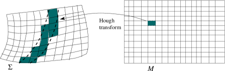
Figure 4: A schematic view of the Hough transform for the discrete case. An observation consists of a pixel in $M$ which goes over to the region enclosed between the dotted lines under the Hough transform. This in turn leads to a selection of pixels in parameter space. The shaded pixels are the ones which get selected and are the ones consistent with the observation.

IV The Hough transform with non-demodulated data

The steps involved in a single incoherent stage of the search are outlined in figure 5. In this search, one starts by breaking up the input data of duration $T_{\textrm{\mbox{\tiny{obs}}}}$ into $N$ segments each with a duration of $T_{\textrm{\mbox{\tiny{coh}}}}$, which would be equal to $T_{\textrm{\mbox{\tiny{obs}}}}/N$ if there were no gaps in the data. Except for precisely two exceptions, namely equations (73) and (116), all the equations in this paper will be valid even in the presence of gaps; we shall not assume $T_{\textrm{\mbox{\tiny{coh}}}}=T_{\textrm{\mbox{\tiny{obs}}}}/N$. This is important because in practice, the real data stream will inevitably have gaps in it representing times when the detector is not in lock or the data is not reliable.

The next step is to compute the Fourier transform of each data segment to obtain $N$ SFTs. Select frequency bins in each SFT by setting a threshold on the normalized power spectrum. This produces a distribution of points in the time-frequency plane — the manifold $M$ — most of which are noise but some excess of which are hopefully present along one or more signal patterns given by equation (4). Having selected points in the time-frequency plane, go through the Hough transform algorithm to obtain the Hough map, i.e. the histogram, in parameter space $\Sigma$. The details follow.

Figure 5: A single stage of a hierarchical continuous wave search involving the Hough transform. The starting point is to break up the data with total observation time $T_{\textrm{\mbox{\tiny{obs}}}}$ into $N$ segments and to compute the Fourier transform of each segment. The next step is to select frequency bins from each SFT by setting a threshold on the normalized power spectrum and use the selected frequency bins to construct a Hough map. The output is then a set of candidates in parameter space obtained by setting a threshold on the Hough number count.

IV.1 Notation and conventions

We assume that the $N$ different data segments have the same time duration. Label the different segments by $a=0,1\ldots(N-1)$ and denote the start time of each segment by $t_{a}$ which will often be called the timestamp of the $a^{th}$ data segment. Let each segment consist of $M$ data points.

Let us now focus on the $a^{th}$ data segment which covers the time interval $[t_{a},t_{a}+T_{\textrm{\mbox{\tiny{coh}}}}]$. Let $x(t)$ be the detector output which is sampled at times $t_{j}=t_{a}+j\Delta t$ with $j=0,1,\ldots(M-1)$. Here the data segment has been subdivided into $M$ sub-segments with the times $t_{j}$ defined to be at the start of each sub-segment; this implies $\Delta t=T_{\textrm{\mbox{\tiny{coh}}}}/M$. Denote the sequence of data points thus obtained by $\{x_{j}\}$ where $x_{j}\equiv x(t_{j})$.

Our convention for the Discrete Fourier Transform (DFT) of $\{x_{j}\}$ is

$$\tilde{x}_{k}=\Delta t\sum_{j=0}^{M-1}x_{j}e^{-2\pi ijk/M}$$ (14)

where $k=0,1\ldots(M-1)$. For $0\leq k\leq\lfloor M/2\rfloor$, the frequency index $k$ corresponds to a physical frequency of $f_{k}=k/T_{\textrm{\mbox{\tiny{coh}}}}$ with $\lfloor.\rfloor$ denoting the integer part of a given real number. The values $\lfloor M/2\rfloor<k\leq M-1$ correspond to negative frequencies given by $f_{k}=(k-M)/T_{\textrm{\mbox{\tiny{coh}}}}$.

The detector output $x(t)$ at any time $t$ is the sum of noise $n(t)$ and a possible gravitational wave signal $h(t)$ of known form:

$$x(t)=n(t)+h(t)\,.$$ (15)

In the remainder of this paper, unless otherwise stated, the stochastic process $n(t)$ is assumed to be stationary and Gaussian with zero mean.

In the continuous case, when the observation time is infinite, the single-sided power spectral density (PSD) $S_{n}(f)$ for $f\geq 0$ is defined as the Fourier transform of the auto-correlation function:

$$S_{n}(f)=2\int_{-\infty}^{\infty}\langle n(t)n(0)\rangle e^{-2\pi ift}dt$$ (16)

where $\langle\cdot\rangle$ denotes the ensemble average.

The normalized power is a dimensionless quantity defined as

$$\rho_{k}=\frac{|\tilde{x}_{k}|^{2}}{\langle|\tilde{n}_{k}|^{2}\rangle}$$ (17)

It can be shown that $\langle|\tilde{n}_{k}|^{2}\rangle$ is related to the PSD:

$$\langle|\tilde{n}_{k}|^{2}\rangle\approx\frac{M\Delta t}{2}S_{n}(f_{k})=\frac{T_{\textrm{\mbox{\tiny{coh}}}}}{2}S_{n}(f_{k})\,.$$ (18)

Thus:

$$\rho_{k}\approx\frac{2|\tilde{x}_{k}|^{2}}{T_{\textrm{\mbox{\tiny{coh}}}}S_{n}(f_{k})}\,.$$ (19)

Naturally, the PSD must be estimated in a way that is not biased by any signal power that may be present.

IV.2 Implementation

The implementation choices we present here mostly correspond to those that have been implemented in the Hough analysis code which is publicly available as part of the LIGO Algorithms Library (LAL) lal , and will be used to analyze the data from the GEO and LIGO detectors.

Restriction on $T_{\textrm{\mbox{\tiny{coh}}}}$: For non-demodulated data, the coherent integration time $T_{\textrm{\mbox{\tiny{coh}}}}$, i.e. the time-baseline of the SFTs, cannot be arbitrarily large. This restriction comes about because we would like the signal power to be concentrated in half a frequency bin but the signal frequency is changing in time due to the Doppler modulation and also due to the spin-down of the star. If $\dot{f}$ is the time-derivative of the signal frequency at any given time, in order for the signal not to shift by more than half a frequency bin, we must have $|\dot{f}|T_{\textrm{\mbox{\tiny{coh}}}}<(2T_{\textrm{\mbox{\tiny{coh}}}})^{-1}$, i.e.

$$T_{\textrm{\mbox{\tiny{coh}}}}<\sqrt{\frac{1}{2|\dot{f}|_{\textrm{\mbox{\tiny{max}}}}}}$$ (20)

where by $|\dot{f}|_{\textrm{\mbox{\tiny{max}}}}$ we mean the maximum possible value of $|\dot{f}|$ for all allowed values of the shape parameters $\vec{\xi}$. The time variation of $f(t)$ is given by equation (4) and is due to two effects: the spin-down of the star, and the Doppler modulation due to the Earth’s motion. We shall assume that the Doppler modulation is the dominant effect . Thus we can estimate $\dot{f}$ by keeping $\hat{f}$ fixed and differentiating ${\bf{v}}(t)$ in equation (4):

$$\dot{f}\approx\frac{\hat{f}}{c}\frac{d{\bf{v}}}{dt}\cdot{\bf{n}}\leq\frac{\hat{f}}{c}\left|\frac{d{\bf v}}{dt}\right|\,.$$ (21)

The important contribution to the acceleration $d{\bf{v}}/dt$ is from the daily rotation of the Earth:

$$|\dot{f}|_{\textrm{\mbox{\tiny{max}}}}=\frac{\hat{f}}{c}\cdot\frac{v_{e}^{2}}{R_{e}}=\frac{\hat{f}}{c}\cdot\frac{4\pi^{2}R_{e}}{T_{e}^{2}}$$ (22)

where $v_{e}$ is the magnitude of the velocity of Earth around its axis, $T_{e}$ the length of a day and $R_{e}$ the radius of Earth. Substituting numerical values we get

$$T_{\textrm{\mbox{\tiny{coh}}}}<50\,\textrm{min}\times\sqrt{\frac{500\,\textrm{Hz}}{\hat{f}}}\,.$$ (23)

In this paper, we shall mostly use $T_{\textrm{\mbox{\tiny{coh}}}}=30$min as the canonical reference value.

Selecting frequency bins: The simplest method of selecting frequency bins is to set a threshold $\rho_{\textrm{\mbox{\tiny{th}}}}$ on $\rho_{k}$; i.e. we select the $k^{th}$ frequency bin if $\rho_{k}\geq\rho_{\textrm{\mbox{\tiny{th}}}}$ and reject it otherwise. Alternatively f ; allen02 , we could impose additional conditions such as requiring that $\rho_{k}>\rho_{k+1}$ and $\rho_{k}>\rho_{k-1}$, i.e. the $k^{th}$ bin is selected if $\rho_{k}$ exceeds the threshold and is, in addition, a local maxima. This can be extended further by including more than just the two neighboring frequency bins. While it is relatively easy to investigate these alternate strategies for non-demodulated data, the analysis becomes more complicated for demodulated data. Furthermore, while these alternate methods might be more robust against spectral disturbances, the analysis of the statistics follows the same general scheme and the results are not qualitatively different. Thus, for the purposes of this paper, we will describe only the simple thresholding scheme for selecting frequency bins. The optimal choice of the threshold $\rho_{\textrm{\mbox{\tiny{th}}}}$ is described below in subsection V.2.

Solving the master equation: As discussed in the previous section, to perform the Hough transform, we must find all the points in parameter space which are consistent with a given observation. In this case, the observation is a frequency $f_{k}$ selected using a threshold $\rho_{\textrm{\mbox{\tiny{th}}}}$ in say, the $a^{th}$ SFT corresponding to a timestamp $t_{a}$. This corresponds to a frequency bin $(f_{k}-\frac{1}{2}\delta f,f_{k}+\frac{1}{2}\delta f)$ where $\delta f=T_{\textrm{\mbox{\tiny{coh}}}}^{-1}$ is the frequency resolution of the SFT. The parameters $\vec{\xi}$ of the signal are the frequency, spin-down parameters, and the sky-positions: $\vec{\xi}=(f_{(0)},\{f_{(n)}\},{\bf{n}})$. Corresponding to $(f_{k}-\frac{1}{2}\delta f,f_{k}+\frac{1}{2}\delta f)$, we must find all the possible values of $\vec{\xi}$ which satisfy the master equation (4).

To understand this better, let us first fix the values of the frequency $f_{(0)}$ and the spin-down parameters $\{f_{(n)}\}$ so that $\hat{f}(t)$ is also fixed. Ignore, for the moment, the frequency resolution $\delta f$. From equation (4), we see that all the values of ${\bf{n}}$ consistent with the observation $f(t)$ must satisfy

$$\cos\phi=\frac{{\bf v}(t)\cdot{\bf{n}}}{v(t)}=\frac{c}{v(t)}\frac{f(t)-\hat{f}(t)}{\hat{f}(t)}$$ (24)

where $\phi$ is the angle between ${\bf v}(t)$ and ${\bf{n}}$. This implies that the angle $\phi$ must be constant; in other words, the set of sky positions consistent with an observation $f(t)$ form a circle in the celestial sphere centered on the vector $\bf{v}$ (see figure 6) . If the frequency $f(t)$ is smeared over a frequency bin $(f_{k}-\frac{1}{2}\delta f,f_{k}+\frac{1}{2}\delta f)$, the set of points consistent with an observation must correspond to an annulus the width $\delta\phi$ of which is easily calculated using equation (24):

$$\delta\phi\approx\frac{c}{v}\frac{\delta f}{\hat{f}\sin\phi}\,.$$ (25)

The annuli are very thick at points where $\sin\phi$ is small, i.e. when ${\bf{n}}$ is almost parallel or anti-parallel to ${\bf v}(t)$ and very thin when perpendicular. This is depicted schematically in figure 6. The circles on the celestial sphere are labeled by an integer $n$ such that the frequency $f=\hat{f}+n\delta f$ corresponds to the angle $\phi_{n}$ given by

$$\cos\phi_{n}=\frac{nc\delta f}{v\hat{f}}\,.$$ (26)

Figure 6: The set of sky positions consistent with a given frequency bin at a given time correspond to annuli on the celestial sphere. These annuli are centered on the velocity vector $\bf{v}$, they are thin when perpendicular to $\bf{v}$ and thick when nearly parallel. The circle with with the label $n=0$ corresponds to $f=\hat{f}$.

The lower limit on the width of the annuli is provided by setting $\phi=\pi/2$ in equation (25):

$$\left(\delta\phi\right)_{\textrm{\mbox{\tiny{min}}}}=\frac{c}{v}\frac{\delta f}{\hat{f}}=\frac{c}{v\hat{f}T_{\textrm{\mbox{\tiny{coh}}}}}$$ (27)

$$=4.8\times 10^{-3}\,\textrm{rad}\times\left(\frac{1\textrm{hr}}{T_{\textrm{\mbox{\tiny{coh}}}}}\right)\left(\frac{500\,\textrm{Hz}}{\hat{f}}\right)\left(\frac{10^{-4}}{v/c}\right)\,.$$

The upper limit on the annuli width $(\delta\phi)_{\textrm{\mbox{\tiny{max}}}}$ is found by setting $\sin\phi\approx\phi\approx(\delta\phi)_{\textrm{\mbox{\tiny{max}}}}$ which gives

$$\left(\delta\phi\right)_{\textrm{\mbox{\tiny{max}}}}=\sqrt{\frac{\delta f}{\hat{f}}\frac{c}{v}}=\sqrt{\frac{c}{v\hat{f}T_{\textrm{\mbox{\tiny{coh}}}}}}$$ (28)

$$=7.3\times 10^{-2}\,\textrm{rad}\times\left(\frac{1\textrm{hr}}{T_{\textrm{\mbox{\tiny{coh}}}}}\right)^{\frac{1}{2}}\left(\frac{500\textrm{Hz}}{\hat{f}}\right)^{\frac{1}{2}}\left(\frac{10^{-4}}{v/c}\right)^{\frac{1}{2}}\,.$$

Therefore, the thick annuli are about $10$ times thicker than the thin ones. Different frequency bins selected at the same time will correspond to non-intersecting annuli as shown in figure 6. However, for frequency bins selected from SFTs at different time stamps, say $t_{a}$ and $t_{b}$, the annuli will usually intersect because the velocity vectors $\bar{\mathbf{v}}(t_{a})$ and $\bar{\mathbf{v}}(t_{b})$ will not, in general, be parallel to each other; see figure 7. p

Figure 7: Two intersecting annuli. The two timestamps $t_{a}$ and $t_{b}$ are sufficiently different from each other so that the velocities $\bar{\mathbf{v}}(t_{a})$ and $\bar{\mathbf{v}}(t_{b})$ are not parallel to each other. This causes the annuli constructed at different timestamps to intersect. The shaded region is the intersection and there is a corresponding region (not shown) on the far side of the sphere.

Resolution in the space of sky-positions: In order to search for pulsar signals in a given portion of the sky, we must choose a tiling for the sky patch. Given the calculation of the annuli width above, we choose the pixel size $\delta\theta$ of the grid to be some fraction, say at most half, of the width $(\delta\phi)_{\textrm{\mbox{\tiny{min}}}}$ of the thinnest annulus. While this educated guess for the pixel size is sufficient for the purposes of this paper, the correct choice of pixel size in the sky patch, and also in the entire parameter space, should use the parameter space metric introduced in owen . The analysis of this metric for the Hough search will be presented elsewhere, and for now we shall simply use $\delta\theta=\frac{1}{2}\,(\delta\phi)_{\textrm{\mbox{\tiny{min}}}}$.

Having selected an annulus and having chosen a tiling on our sky-patch, we now need a criterion for selecting a pixel if it intersects an annulus. Our criterion is to select a pixel if its center lies within an annulus. Under such a criterion, a given pixel can then be selected by at most one annulus and the pixels selected by all the annuli together will exactly cover the sphere.

Resolution in the space of spin-down parameters: In the absence of a proper analysis of the parameter space metric, we shall just use the obvious estimate for the resolution $\delta f_{(n)}$:

$$\delta f_{(n)}=n!\frac{\delta f}{T_{\textrm{\mbox{\tiny{obs}}}}^{n}}\,.$$ (29)

As an example, for the first spin-down parameter:

$$\delta f_{(1)}=(2.1\times 10^{-10}\textrm{Hz/s})\times\frac{30\textrm{days}}{T_{\textrm{\mbox{\tiny{obs}}}}}\cdot\frac{1800\textrm{s}}{T_{\textrm{\mbox{\tiny{coh}}}}}\,.$$ (30)

We now need to choose the range of values $-f_{(n)}^{\textrm{\mbox{\tiny{max}}}}<f_{(n)}<f_{(n)}^{\textrm{\mbox{\tiny{max}}}}$ and the largest number of spin-down parameters $s_{\textrm{\mbox{\tiny{max}}}}$ to be searched over. Assuming that the pulsar’s frequency evolution is well-represented by a Taylor expansion, we get

$$f_{(n)}^{\textrm{\mbox{\tiny{max}}}}=n!\frac{\hat{f}_{\textrm{\mbox{\tiny{max}}}}}{\tau^{n}}$$ (31)

where $\tau$ is the age of the pulsar and $\hat{f}_{\textrm{\mbox{\tiny{max}}}}$ is the largest intrinsic frequency that we search over. We include the $n^{th}$ spin-down parameter in our search only if the resolution defined by equation (29) is not too coarse compared to $f_{(n)}^{\textrm{\mbox{\tiny{max}}}}$:

$$\delta f_{(n)}<f_{(n)}^{\textrm{\mbox{\tiny{max}}}}\,.$$ (32)

Since $T_{\textrm{\mbox{\tiny{obs}}}}\ll\tau$, $f_{(n)}^{\textrm{\mbox{\tiny{max}}}}$ decreases with increasing $n$ much faster than $\delta f_{(n)}$; this implies that there must exist a value $s_{\textrm{\mbox{\tiny{max}}}}$ such that equation (32) is satisfied for all $n\leq s_{\textrm{\mbox{\tiny{max}}}}$ and is violated for all $n>s_{\textrm{\mbox{\tiny{max}}}}$. Any spin-down parameter of order greater than $s_{\textrm{\mbox{\tiny{max}}}}$ does not significantly affect the result of the Hough transform. As an example, if we wish to search for pulsars whose age is at least $\tau=40$yrs, then for $\hat{f}_{\textrm{\mbox{\tiny{max}}}}=1000$Hz, it is easy to check that we get $s_{\textrm{\mbox{\tiny{max}}}}=3$. In other words, to look for pulsars which are as young as $40$yr, we must include at least 3 spin-down parameters in our search.

On the other hand, in some cases, computational requirements might dictate that we can only search over, say, one spin-down parameter. This automatically sets a lower limit on the age of the pulsar that we can search over because then the second spin-down parameter must satisfy $\delta f_{(2)}>f_{(2)}^{\textrm{\mbox{\tiny{max}}}}$ which leads to

$$\tau>155\textrm{yr}\times\frac{T_{\textrm{\mbox{\tiny{obs}}}}}{30\textrm{days}}\cdot\left(\frac{\hat{f}_{\textrm{\mbox{\tiny{max}}}}}{1000\textrm{Hz}}\cdot\frac{T_{\textrm{\mbox{\tiny{coh}}}}}{1800\textrm{s}}\right)^{1/2}\,.$$ (33)

Finally, the finite length of $T_{\textrm{\mbox{\tiny{coh}}}}$ itself leads to a lower bound on $\tau$. If $f_{(n)}$ is too large, then the signal power may no longer be concentrated in a single frequency bin and the assumption of neglecting spin-down parameters which was used to derive equation (23) will no longer be valid. To be certain that the spin-down will not cause the signal to move by more than half a frequency bin, we must have $f_{(n)}^{\textrm{\mbox{\tiny{max}}}}T_{\textrm{\mbox{\tiny{coh}}}}^{n}<n!\delta f/2$ which implies

$$\tau>\left(\frac{2\hat{f}_{\textrm{\mbox{\tiny{max}}}}T_{\textrm{\mbox{\tiny{coh}}}}^{n+1}}{n!}\right)^{1/n}\,.$$ (34)

The most stringent limit is obtained for $n=1$:

$$\tau>103\textrm{yr}\times\frac{\hat{f}_{\textrm{\mbox{\tiny{max}}}}}{1000\textrm{Hz}}\left(\frac{T_{\textrm{\mbox{\tiny{coh}}}}}{1800\textrm{s}}\right)^{2}\,.$$ (35)

This restriction will not be present if we use demodulated data as input for the Hough transform.

Partial and total Hough maps: As described above, for a given frequency bin selected at a given time-stamp and for a given value of the instantaneous frequency $\hat{f}$, we can find the set of sky locations which are consistent with the master equation (4). In other words, every pixel in the sky-patch either gets selected or rejected and this gives a histogram in the $(\alpha,\delta)$ plane consisting of ones or zeros; $\alpha$ and $\delta$ are coordinates on the sky-patch. Such a collection of ones and zeros on the sky-patch is called a Partial Hough Map (PHM). The number of PHMs required at any given time depends on the frequency band $\Delta f_{b}$ that one is searching over and is given by $\Delta f_{b}/\delta f=T_{\textrm{\mbox{\tiny{obs}}}}\Delta f_{b}$.

Given a set of PHM’s for every time interval, and given a set of spin-down parameters that one wishes to search for, the Total Hough Map (THM) is obtained by summing the appropriate partial Hough maps.

Figure 8: A Partial Hough Map (PHM) is a histogram in the $(\alpha,\delta)$ plane constructed from all the frequencies selected at a given time and for a given value of the instantaneous frequency $\hat{f}_{0}$. A total Hough map is obtained by summing over the appropriate Hough maps. The PHMs to be summed over are determined by the choice of spin-down parameters which give a trajectory in the time-frequency plane. For example, a single spin down parameter will give a straight line as shown is the figure while two spin-down parameters will lead to a parabola.

To see how this comes about, consider the case when we are searching for some spin-down parameters $\{f_{(n)}\}$ with $n=1,2,\cdots$. The instantaneous frequency changes with time according to equation (5); ignore the $\Delta\mathbf{r}$ term in this equation . This can be viewed as a trajectory in the time-frequency plane. A single spin-down parameter will give a straight line, two spin-down parameters a parabola and so on. Thus for each time-stamp $t_{a}$, we can find the appropriate PHM by looking at which frequency bin this trajectory intersects (see figure 8). For a given choice of spin-down parameters, the THM is obtained by summing over the appropriate PHMs. Repeating this for every set of frequency and spin-down parameters we wish to search over, we obtain a number of THMs and the collection of all these THMs represent our final histogram in parameter space.

Look up tables: The procedure described thus far is, in principle, enough to produce a complete Hough map in parameter space. However, it is possible to enormously reduce the computational cost by using Look Up Tables (LUTs) which we now describe. Assume that we have managed to find all the annuli for a given time-stamp $t_{a}$ and for a given search frequency $\hat{f}$. To construct the PHM for $t_{a}$ and $\hat{f}$, we just need to select the appropriate annuli out of all the ones that we have found. Very importantly, it turns out that in most cases, the annuli are relatively insensitive to changes in $\hat{f}$ and can therefore be re-used a large number of times.

To see this, look at how the solutions of equation (4) depend on the search frequency $\hat{f}$. We want to calculate the maximum number $\kappa$ of frequency bins that $\hat{f}$ can be changed by so that the annuli change by only a fraction $r$ of the quantity $(\delta\phi)_{\textrm{min}}$ defined in equation (IV.2). As discussed earlier, if we restrict ourselves to discrete frequencies, the annuli corresponding to every given value of $\hat{f}$ are parameterized by an integer $n$ according to equation (26). For a fixed value of $n$, by how much does $\phi_{n}$ change when $\hat{f}$ is varied? To answer this, differentiate equation (26) with respect to $\hat{f}$:

$$\frac{d\hat{f}}{\hat{f}^{2}}=\frac{1}{n\delta f}\frac{v}{c}\sin\phi_{n}\,d\phi_{n}=\frac{\tan\phi_{n}}{\hat{f}}d\phi_{n}\,.$$ (36)

Set $d\phi_{n}=r(\delta\phi)_{\textrm{\mbox{\tiny{min}}}}$ and $d\hat{f}=\kappa\delta f=\kappa/T_{\textrm{\mbox{\tiny{coh}}}}$ to obtain

$$\kappa=\frac{rc}{v}\tan\phi_{n}=\frac{rc}{v}\sqrt{\frac{n_{0}^{2}}{n^{2}}-1}$$ (37)

where $n_{0}=v\hat{f}/(c\delta f)$. Consider separately the two regimes when $\phi_{n}\sim\pi/2$ (i.e. $n\sim 0$) and $\phi_{n}\sim 0,\pi$ (i.e. $n\sim\pm n_{0}$). When $\phi_{n}=\pi/2$, then $\kappa$ is infinite which indicates that a LUT is excellent in this regime. On the other hand, $\kappa=0$ for $\phi_{n}=0,\pi$. However, since the resolution in $\phi$ is finite, instead of $\phi_{n}=0$, it is more appropriate to take the worst case scenario as $\phi_{n}=(\delta\phi)_{\textrm{\mbox{\tiny{min}}}}$ so that

$$\kappa\approx\frac{rc}{v}\left(\delta\phi\right)_{\textrm{\mbox{\tiny{min}}}}=40r\left(\frac{500\,\textrm{Hz}}{\hat{f}}\right)^{\frac{1}{2}}\,.$$ (38)

Thus, in this worst case scenario, for a frequency of 500 Hz and a tolerance of $r=0.1$, the LUT will be valid for $4$ frequency bins. Furthermore, due to the presence of the function $\tan\phi$ in equation (37), $\kappa$ increases rapidly with increasing $\phi_{n}$ (i.e. decreasing $n$). As an example, take $T_{\textrm{\mbox{\tiny{coh}}}}=1800$s, $\hat{f}=500$ Hz, and $v/c=10^{-4}$ so that $n_{0}=90$. Then, even for $n=89$, we get $\kappa=1500r$; thus with say $r=0.1$, the LUT is valid for about $150$ frequency bins.

The main point of using the look up tables and partial Hough maps is to reduce the computational costs. Assume that we are searching over a frequency band $\Delta f_{b}$, let $N_{p}$ be the number of templates in the space of sky-locations and spin-down parameters; $T_{\textrm{\mbox{\tiny{coh}}}}\Delta f_{b}$ is the number of frequency bins being searched over.

A naive implementation of the Hough transform will require, for every point in parameter space, to identify first the corresponding pattern in the time-frequency plane and then add $N$ integers (zeros or ones) to obtain the final number count, where $N$ is the number of data segments. If we use LUTs, which are valid for a large number of search frequencies, their computational cost in the search becomes negligible, i.e. the cost of finding the patterns is negligible, and the number of floating point operations required is thus $C_{0}\approx T_{\textrm{\mbox{\tiny{coh}}}}\Delta f_{b}N_{p}N$. This calculation can be organized much more efficiently if we perform a search on many sky locations at once. In this case, if we know the locations of all the annuli, for every chosen frequency bin, we mark the corresponding annulus and in the end, combine all the annuli thus selected to get the final number count. The exact savings in computational cost due to this strategy are implementation dependent, but are typically better by a factor of $\sim 5$ when compared to the value $C_{0}$ mentioned above. This factor is related to the number of frequency bins selected from each SFT.

V Statistical properties of the Hough maps

This section is divided into three parts: The probability distribution of the number counts is calculated in subsection V.1, subsection V.2 optimizes the various thresholds and subsection V.3 estimates the sensitivity of the Hough search.

V.1 The number count distribution

The frequency bins that are fed into the Hough transform are the ones such that their normalized power $\rho_{k}$ defined in equation (17) exceeds a threshold $\rho_{\textrm{\mbox{\tiny{th}}}}$. Assuming that the noise is stationary, has zero mean, and is Gaussian, from equation (17), we get

$$2\rho_{k}=z_{1}^{2}+z_{2}^{2}$$ (39)

where

$$z_{1}=\frac{\sqrt{2}\textrm{Re}[\tilde{x}_{k}]}{\sqrt{\langle|\tilde{n}_{k}|^{2}\rangle}}\qquad\textrm{and}\qquad z_{2}=\frac{\sqrt{2}\textrm{Im}[\tilde{x}_{k}]}{\sqrt{\langle|\tilde{n}_{k}|^{2}\rangle}}\,.$$ (40)

As before, the detector output $\tilde{x}_{k}$ is the sum of noise and a possible signal: $\tilde{x}_{k}=\tilde{n}_{k}+\tilde{h}_{k}$. Assuming that $\textrm{Re}[\tilde{n}_{k}]$ and $\textrm{Im}[\tilde{n}_{k}]$ are independent random variables with equal variance, it is easy to show that their variance must be equal to $\langle|\tilde{n}_{k}|^{2}\rangle/2$. Therefore, taking the noise to be Gaussian, it follows that the random variables $z_{1}$ and $z_{2}$ are normally distributed and have unit variance (but non-zero mean). Thus $2\rho_{k}$ must be distributed according to a non-central $\chi^{2}$ distribution with 2 degrees of freedom with non-centrality parameter $\lambda_{k}$:

$$\lambda_{k}=\left(\mathbf{E}[z_{1}]\right)^{2}+\left(\mathbf{E}[z_{2}]\right)^{2}=\frac{4|\tilde{h}(f_{k})|^{2}}{T_{\textrm{\mbox{\tiny{coh}}}}S_{n}(f_{k})}\,.$$ (41)

Thus the distribution of $\rho_{k}$ is

$$p\left(\rho_{k}|\lambda_{k}\right) = 2\chi^{2}(2\rho_{k}|\,2,\lambda_{k})$$ (42)

$$= \exp\left(-\rho_{k}-\frac{\lambda_{k}}{2}\right)I_{0}(\sqrt{2\lambda_{k}\rho_{k}})$$

where $I_{0}$ is the modified Bessel’s function of zeroth order. As expected, $p\left(\rho_{k}|\lambda_{k}\right)$ reduces to the exponential distribution in the absence of a signal (when $\lambda=0$).

The mean and variance for this distribution are respectively

$$\mathbf{E}[\rho_{k}]=1+\frac{\lambda_{k}}{2}\qquad\textrm{and}\qquad\mathbf{\sigma^{2}}[\rho_{k}]=1+\lambda_{k}\,.$$ (43)

The probability $\eta$ that a given frequency bin is selected is

$$\eta(\rho_{\textrm{\mbox{\tiny{th}}}}|\lambda)=\int_{\rho_{\textrm{\mbox{\tiny{th}}}}}^{\infty}p(\rho|\lambda)\,\textrm{d}\rho$$ (44)

where we have dropped the subscript $k$ for notational simplicity; it is understood that $\rho$ and $\lambda$ always refer to one of the Fourier frequency bins. The false alarm and false dismissal probabilities for the frequency bin selection are respectively

$$\alpha(\rho_{\textrm{\mbox{\tiny{th}}}}) = \int_{\rho_{\textrm{\mbox{\tiny{th}}}}}^{\infty}p(\rho|0)\,\textrm{d}\rho=e^{-\rho_{\textrm{\mbox{\tiny{th}}}}}\,,$$ (45)

$$\beta(\rho_{\textrm{\mbox{\tiny{th}}}}|\lambda) = 1-\eta(\rho_{\textrm{\mbox{\tiny{th}}}}|\lambda)=\int_{0}^{\rho_{\textrm{\mbox{\tiny{th}}}}}p(\rho|\lambda)\,\textrm{d}\rho\,.$$ (46)

Clearly, $\eta=\alpha$ when no signal is present and $\eta$ becomes larger when the signal becomes stronger and $\eta\rightarrow 1$ when $\lambda\rightarrow\infty$. Figure 9 shows $\eta(\rho_{\textrm{\mbox{\tiny{th}}}}|\lambda)$ as a function of the non-centrality parameter $\lambda$ for two different values of $\rho_{\textrm{\mbox{\tiny{th}}}}$. For small $\lambda$:

$$\eta(\rho_{\textrm{\mbox{\tiny{th}}}}|\lambda)=\alpha\left\{1+\frac{\rho_{\textrm{\mbox{\tiny{th}}}}}{2}\lambda+\mathcal{O}(\lambda^{2})\right\}\,.$$ (47)

This expansion will be very useful when we restrict ourselves to the case of small signals.

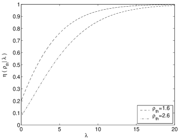
Figure 9: Plot the detection probability $\eta(\rho_{\textrm{\mbox{\tiny{th}}}}|\lambda)$ as a function of $\lambda$ for $\rho_{\textrm{\mbox{\tiny{th}}}}=1.6$ and $2.6$.

In the presence of a signal, the non-centrality parameter $\lambda_{k}$ is not constant across different SFTs. The reason for this is two-fold: First, the noise may be significantly non-stationary. Secondly, and more fundamentally, the observed signal power $|\tilde{h}|^{2}$ changes because of the amplitude modulation of the signal caused by the non-uniform antenna pattern of the detector. Therefore, the detection probability $\eta$ changes across SFTs. In what follows, we shall neglect this effect and take $\lambda$ and $\eta$ to be constant for different SFTs.

Under this assumption, the probability of measuring a number count $n$ in a pixel of a Hough map constructed from $N$ SFTs is given by the binomial distribution:

$$p(n|\rho_{\textrm{\mbox{\tiny{th}}}},\lambda)=\left(\begin{array}[]{c}N\\ n\end{array}\right)\eta^{n}(1-\eta)^{N-n}\,.$$ (48)

The mean and variance of the number count are respectively

$$\bar{n}=N\eta\qquad\textrm{and}\qquad\sigma^{2}=N\eta(1-\eta)\,.$$ (49)

In the absence of a signal, $\eta=\alpha$ so that

$$p(n|\rho_{\textrm{\mbox{\tiny{th}}}},0)=\left(\begin{array}[]{c}N\\ n\end{array}\right)\alpha^{n}(1-\alpha)^{N-n}\,.$$ (50)

Candidates for detection or for further analysis are selected by setting a threshold $n_{\textrm{\mbox{\tiny{th}}}}$ on the number count. Based on this, we can define the false alarm and false dismissal rates respectively as:

$$\alpha_{H}(n_{\textrm{\mbox{\tiny{th}}}},\rho_{\textrm{\mbox{\tiny{th}}}},N) = \sum_{n=n_{\textrm{\mbox{\tiny{th}}}}}^{N}p(n|\rho_{\textrm{\mbox{\tiny{th}}}},0)\,,$$ (51)

$$\beta_{H}(n_{\textrm{\mbox{\tiny{th}}}},\rho_{\textrm{\mbox{\tiny{th}}}},\lambda,N) = \sum_{n=0}^{n_{\textrm{\mbox{\tiny{th}}}}-1}p(n|\rho_{\textrm{\mbox{\tiny{th}}}},\lambda)\,.$$ (52)

These two quantities determine the significance and the sensitivity of the Hough search and will play an important role in the rest of this paper.

V.2 Optimal choice of the thresholds

In order to carry out the Hough search, we have to set two thresholds: the threshold $\rho_{\textrm{\mbox{\tiny{th}}}}$ on the normalized power and the threshold $n_{\textrm{\mbox{\tiny{th}}}}$ on the number count.

The value of $n_{\textrm{\mbox{\tiny{th}}}}$ is determined by the false alarm rate $\alpha_{H}^{\star}$ that depends on the number of candidates that we can feasibly follow up.

The value of $\rho_{\textrm{\mbox{\tiny{th}}}}$ is chosen in such as way so as to make the search as powerful as possible. We present two criteria that yield the same result for small signals and for large $N$.

Maximizing the critical ratio: For the Hough number count, we can define a random variable called the critical ratio as follows

$$\Psi=\frac{n-N\alpha}{\sqrt{N\alpha(1-\alpha)}}\,,$$ (53)

This quantity is a measure of the “significance” of a measured value $n$ with respect to the expected value $N\alpha$ in the absence of any signal, weighted by the expected fluctuations of the noise. In the presence of a signal, the expected value of the critical ratio is

$$\bar{\Psi}(\eta,\alpha)=\frac{N\eta-N\alpha}{\sqrt{N\alpha(1-\alpha)}}\,,$$ (54)

Recall that $\eta$ and $\alpha$ depend on the threshold $\rho_{\textrm{\mbox{\tiny{th}}}}$ according to equations (45) and (46) respectively. Thus, our criterion for choosing the threshold is to maximize $\bar{\Psi}(\eta,\alpha)$ with respect to $\rho_{\textrm{\mbox{\tiny{th}}}}$. In the case of small signals where $\eta\approx\alpha(1+\rho_{\textrm{\mbox{\tiny{th}}}}\lambda/2)$, the condition

$$\frac{\partial\bar{\Psi}}{\partial\rho_{\textrm{\mbox{\tiny{th}}}}}=0$$ (55)

leads to

$$\ln\alpha=2(\alpha-1)$$ (56)

which yields $\rho_{\textrm{\mbox{\tiny{th}}}}\approx 1.6$ or equivalently, $\alpha\approx 0.20$.

The Neyman-Pearson criterion: An alternative method of choosing $\rho_{\textrm{\mbox{\tiny{th}}}}$ is based on the Neyman-Pearson criterion which tells us to minimize the false dismissal rate $\beta_{H}$ for a given value $\alpha_{H}^{\star}$ of the false alarm rate. For weak signals, this requirement uniquely determines $\rho_{\textrm{\mbox{\tiny{th}}}}$ and, as we shall see, this agrees with the previous criterion.

In practice, taking $N$ and $\lambda$ to be fixed parameters, this is the procedure:

i.

First choose a value $\alpha_{H}^{\star}$ for the largest false alarm rate $\alpha_{H}$ that we can allow.

ii.

Invert the equation $\alpha_{H}(\rho_{\textrm{\mbox{\tiny{th}}}},N,n_{\textrm{\mbox{\tiny{th}}}})\leq\alpha_{H}^{\star}$ to obtain $n_{\textrm{\mbox{\tiny{th}}}}(\rho_{\textrm{\mbox{\tiny{th}}}},N,\alpha_{H}^{\star})$.

iii.

Substitute the value of $n_{\textrm{\mbox{\tiny{th}}}}$ thus obtained in the expression for the false dismissal $\beta_{H}(n_{\textrm{\mbox{\tiny{th}}}},\rho_{\textrm{\mbox{\tiny{th}}}},\lambda,N)$. This gives $\beta_{H}$ as a function of $(\rho_{\textrm{\mbox{\tiny{th}}}},\lambda,N,\alpha_{H}^{\star})$.

iv.

Minimize $\beta_{H}$ as a function of $\rho_{\textrm{\mbox{\tiny{th}}}}$. Let $\rho_{\textrm{\mbox{\tiny{th}}}}^{\star}$ be the value that minimizes $\beta_{H}$.

v.

Using $n_{\textrm{\mbox{\tiny{th}}}}(\rho_{\textrm{\mbox{\tiny{th}}}},N,\alpha_{H}^{\star})$ derived in step (ii) above, obtain $n_{\textrm{\mbox{\tiny{th}}}}^{\star}=n_{\textrm{\mbox{\tiny{th}}}}(\rho_{\textrm{\mbox{\tiny{th}}}}^{\star},N,\alpha_{H}^{\star})$.

This procedure is also applicable if we choose a different method of selecting frequency bins other than simple thresholding, such as, for example the peak selection criterion mentioned towards the end of subsection IV.1.

The results of the optimization procedure described above are shown in figures 10, 11 and 12. Figure 10 shows the value of the number count threshold $n_{\textrm{\mbox{\tiny{th}}}}$ obtained as described in step (ii). In this figure, instead of $\rho_{\textrm{\mbox{\tiny{th}}}}$, we have chosen the false alarm rate $\alpha=e^{-\rho_{\textrm{\mbox{\tiny{th}}}}}$ as the independent variable; $\alpha$ is the false alarm rate for selecting frequency bins and is not to be confused with $\alpha_{H}$. Figure 10 also shows an analytic approximation to $n_{\textrm{\mbox{\tiny{th}}}}$ obtained below in equation (59). Using this result for $n_{\textrm{\mbox{\tiny{th}}}}$, figure 11 shows $\beta_{H}$ as a function of $\alpha=e^{-\rho_{\textrm{\mbox{\tiny{th}}}}}$. The optimal choice $\rho_{\textrm{\mbox{\tiny{th}}}}^{\star}$ of $\rho_{\textrm{\mbox{\tiny{th}}}}$ is when $\beta_{H}$ is a minimum and, for small signals, this happens at $\rho_{\textrm{\mbox{\tiny{th}}}}^{\star}\approx 1.6$ which corresponds to $\alpha^{\star}:=e^{-\rho_{\textrm{\mbox{\tiny{th}}}}^{\star}}\approx 0.20$ . Finally, figure 12 shows the minimum value of $\beta_{H}$ obtained by this optimization as a function of the signal strength $\lambda$ and for two different values of $N$.

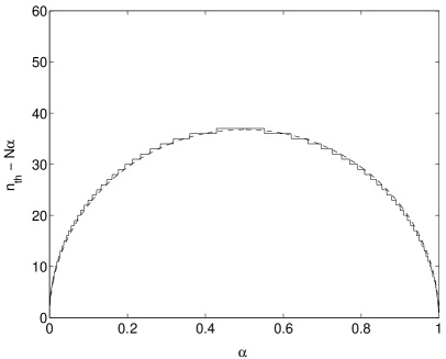
Figure 10: Graph of $n_{\textrm{\mbox{\tiny{th}}}}-N\alpha$ versus the false alarm probability $\alpha=e^{-\rho_{\textrm{\mbox{\tiny{th}}}}}$ for $\alpha_{H}=0.01$ and $N=2000$. The dashed line shows the analytic approximation given by equation (59).

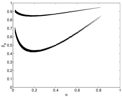
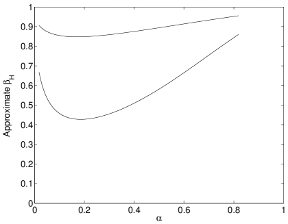
Figure 11: The first figure shows the Hough false dismissal rate as a function of the false alarm rate $\alpha=e^{-\rho_{\textrm{\mbox{\tiny{th}}}}}$ for a non-centrality parameter $\lambda=0.10$ (upper curve) and $\lambda=0.20$ (lower curve). Both curves correspond to $\alpha_{H}=0.01$ and $N=1000$. The minimum values of $\beta_{H}$ for the two curves are approximately $0.84$ and $0.41$ respectively. Both minima occur at $\alpha=0.20$ approximately. This corresponds to a threshold of $\rho_{\textrm{\mbox{\tiny{th}}}}=1.6$ on the normalized power statistic. The bottom figure shows the approximation to $\beta_{H}$ using equations (V.2) and (59) with the same parameters as in the first figure.

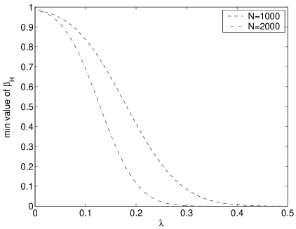
Figure 12: Minimum value of $\beta_{H}$ as a function of the non-centrality parameter $\lambda$ for $\alpha_{H}=0.01$ and for $N=1000$ and $2000$. As expected, a larger value of $N$ typically leads to a smaller value of $\beta_{H}$.

The Gaussian approximation: To better understand the statistics, it is useful to carry out the above steps analytically by taking $n$ to be a continuous variable and by approximating the binomial distribution by a Gaussian with the appropriate mean and variance:

$$p(n|\rho_{\textrm{\mbox{\tiny{th}}}},\lambda)=\frac{1}{\sqrt{2\pi\sigma^{2}}}e^{-(n-N\eta)^{2}/2\sigma^{2}}\,.$$ (57)

This is a very good approximation when $N$ is large and $\eta$ is not too close to $0$ or $1$. If $n$ is chosen to lie within $[0,N]$, the distribution is properly normalized only approximately. For simplicity, in what follows we shall take the range of $n$ to be $(-\infty,+\infty)$; this is an excellent approximation if the above assumptions on $N$ and $\eta$ hold.

With the approximations given above, we can rewrite the equation $\alpha_{H}=\alpha_{H}^{\star}$ as

$$\int_{n_{\textrm{\mbox{\tiny{th}}}}}^{\infty}p(n|\rho_{\textrm{\mbox{\tiny{th}}}},0)\,dn=\alpha_{H}^{\star}\,.$$ (58)

The solution to this equation can be rewritten in terms of the complementary error function:

$$n_{\textrm{\mbox{\tiny{th}}}}(\rho_{\textrm{\mbox{\tiny{th}}}},N,\alpha_{H}^{\star})=N\alpha+\sqrt{2N\alpha(1-\alpha)}\,\,\textrm{erfc}^{-1}(2\alpha_{H}^{\star})\,.$$ (59)

As shown in figure 10, this is a very good approximation to the actual value of $n_{\textrm{\mbox{\tiny{th}}}}$ obtained from the binomial distribution.

The expression for $\beta_{H}$ is similarly rewritten as

$$\beta_{H}=\frac{1}{2}\textrm{erfc}\left(\frac{N\eta-n_{\textrm{\mbox{\tiny{th}}}}}{\sqrt{2N\eta(1-\eta)}}\right)\,.$$

As figure 11 shows, this too is a very good approximation to $\beta_{H}$ obtained using the binomial distribution.

In step (iv), we find $\rho_{\textrm{\mbox{\tiny{th}}}}^{\star}$ such that

$$\left.\frac{\partial\beta_{H}}{\partial\rho_{\textrm{\mbox{\tiny{th}}}}}\right|_{\rho_{\textrm{\mbox{\tiny{th}}}}=\rho_{\textrm{\mbox{\tiny{th}}}}^{\star}}=0$$ (60)

In the case of small signals where $\eta\approx\alpha(1+\rho_{\textrm{\mbox{\tiny{th}}}}\lambda/2)$, the solution to the above equation becomes independent of $\lambda$, and it is also independent of $N$ when $N$ is large. In these limits, the solution is given by

$$\left.\frac{\partial}{\partial\rho_{\textrm{\mbox{\tiny{th}}}}}\left(\sqrt{\frac{\rho_{\textrm{\mbox{\tiny{th}}}}^{2}}{e^{\rho_{\textrm{\mbox{\tiny{th}}}}}-1}}\right)\right|_{\rho_{\textrm{\mbox{\tiny{th}}}}=\rho_{\textrm{\mbox{\tiny{th}}}}^{\star}}=0\,.$$ (61)

The solution to this equation is $\rho_{\textrm{\mbox{\tiny{th}}}}^{\star}\approx 1.6$ and $\alpha^{\star}=e^{-\rho_{\textrm{\mbox{\tiny{th}}}}^{\star}}\approx 0.20$. Notice that this equation is equivalent to equation (55) and furthermore, the functions being extremized are rather flat near the extremum. Thus, the threshold could be chosen somewhat differently without significantly impacting the sensitivity. In particular, the threshold can be increased so that fewer frequency bins are selected. Depending on the details of the implementation, this could lead to a lower computational cost; in the framework of a hierarchical search, this will improve the overall sensitivity.

Finally, with the optimal threshold $\rho_{\textrm{\mbox{\tiny{th}}}}^{\star}$ at hand, the optimal threshold $n_{\textrm{\mbox{\tiny{th}}}}^{\star}$ on the number count is obtained by substituting $\rho_{\textrm{\mbox{\tiny{th}}}}=\rho_{\textrm{\mbox{\tiny{th}}}}^{\star}$ in equation (59):

$$n_{\textrm{\mbox{\tiny{th}}}}^{\star} = n_{\textrm{\mbox{\tiny{th}}}}(\rho_{\textrm{\mbox{\tiny{th}}}}^{\star},N,\alpha_{H}^{\star})$$

$$= N\alpha^{\star}+\sqrt{2N\alpha^{\star}(1-\alpha^{\star})}\,\textrm{erfc}^{-1}(2\alpha_{H}^{\star})\,.$$

This is an important equation because it tells us the number count threshold that must be set in order to have a given number of follow-up candidates.

V.3 Sensitivity

In this subsection, we estimate the sensitivity of the Hough search, i.e. we answer the following question: for given values $\alpha_{H}^{\star}$ and $\beta_{H}^{\star}$ of the false alarm $\alpha_{H}$ and false dismissal $\beta_{H}$ respectively, what is the smallest value of the gravitational wave amplitude $h_{0}$ (see equation (9)) that would cross the thresholds $\rho_{\textrm{\mbox{\tiny{th}}}}$ and $n_{\textrm{\mbox{\tiny{th}}}}$? Equivalently, for a given false alarm rate $\alpha_{H}^{\star}$, what is the smallest $h_{0}$ which will give a false dismissal rate of at least $\beta_{H}^{\star}$? We use the signal model of equation (7) and we present our final result for the values $\alpha_{H}=\alpha_{H}^{\star}=0.01$ and $\beta_{H}=\beta_{H}^{\star}=0.10$. The value of $0.01$ is meant mainly for illustration purposes and does not change the results qualitatively. Furthermore, for comparison, equation (2.2) in S1:pulsar assumes a false alarm of $0.01$ and this choice of $\alpha_{H}^{\star}$ enables an easier comparison with that result. As far as possible, we explicitly retain the factors of $\alpha_{H}^{\star}$ in our equations substituting numerical values only when necessary.

We must first solve the equation

$$\beta_{H}(n_{\textrm{\mbox{\tiny{th}}}}^{\star},\rho_{\textrm{\mbox{\tiny{th}}}}^{\star},\lambda,N)=\beta_{H}^{\star}$$ (63)

and obtain $\lambda$ as a function of $N$; this will yield the desired value of $h_{0}$.

In order to simplify the discussion, we shall again approximate the binomial distribution by a normal distribution whose mean $\bar{n}$, and variance $\sigma$, are respectively given by equation (49). The false dismissal rate is

$$\beta_{H}\approx\frac{1}{2}\textrm{erfc}\left(\frac{\bar{n}-n_{\textrm{\mbox{\tiny{th}}}}^{\star}}{\sqrt{2N\eta^{\star}(1-\eta^{\star})}}\right)$$ (64)

where $n_{\textrm{\mbox{\tiny{th}}}}^{\star}$ is as given in equation (59) and $\eta^{\star}=\eta(\rho_{\textrm{\mbox{\tiny{th}}}}^{\star}|\lambda)$.

Since we are interested in the case of small signals, let us approximate $\eta$ by only keeping terms of the order of $\lambda$ in equation (47). Ignoring terms of $\mathcal{O}(\lambda^{2})$, equation (64) leads to the approximation

$$\beta_{H}=\frac{1}{2}\textrm{erfc}\left(-\textrm{erfc}^{-1}(2\alpha_{H}^{\star})+\frac{1}{2}\Theta\alpha^{\star}\rho_{\textrm{\mbox{\tiny{th}}}}^{\star}\lambda\right)$$ (65)

where

$$\Theta=\sqrt{\frac{N}{2\alpha^{\star}(1-\alpha^{\star})}}+\left(\frac{1-2\alpha^{\star}}{1-\alpha^{\star}}\right)\frac{\textrm{erfc}^{-1}(2\alpha_{H}^{\star})}{2\alpha^{\star}}\,.$$ (66)

Let us summarize our approximation scheme for $\beta_{H}$. The first approximation is to take the number count distribution to be binomial. The second approximation is in equation (64) which replaces the binomial by a Gaussian distribution with the appropriate mean and variance. The final approximation is in equation (65) where we have taken $\lambda$ to be small and used a Taylor series in powers of $\lambda$ retaining only the linear term. To get a feeling for the validity of these approximations, figure 13 shows graphs of $\beta_{H}$ as a function of $\lambda$ for different values of $N$. As the graphs show, we can trust the approximations when $N\sim 10^{3}$. For smaller values of $N$, while the Gaussian approximation is still reasonable, the linear approximation greatly under-estimates $\beta_{H}$ for a given value of $\lambda$, i.e. it make the Hough search appear more sensitive than it actually is.

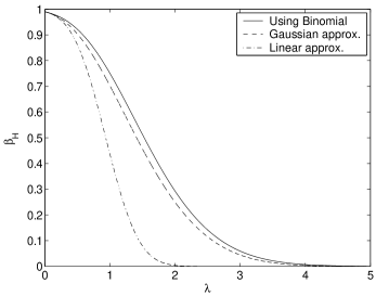
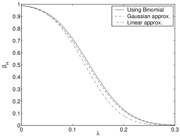
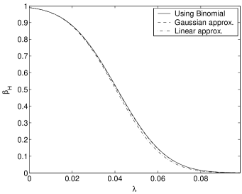
Figure 13: Graphs of $\beta_{H}$ as a function of $\lambda$ for different values of $N$ and for the three different approximations used. In the first panel $N=20$, the second panel has $N=2000$ and in the third panel, $N=20,000$. All graphs are plotted assuming the optimal values for $\rho_{\textrm{\mbox{\tiny{th}}}}$ and $n_{\textrm{\mbox{\tiny{th}}}}$. The linear approximation is clearly unacceptable for $N\sim 10^{1}$ but becomes reasonable when $N\sim 10^{2}$ or $10^{3}$ and is excellent for $N\sim 10^{4}$. The Gaussian approximation is clearly much better and is good even for $N=20$. Finally, note that the approximations always underestimate the value of $\beta_{H}$.

Working with the linear approximation of equation (65), assuming $N$ to be very large and $\textrm{erfc}^{-1}(2\alpha_{H}^{\star})\ll N$, set $\beta_{H}=\beta_{H}^{\star}$ and solve for $\lambda$:

$$\lambda\approx\frac{\mathcal{S}}{\rho_{\textrm{\mbox{\tiny{th}}}}^{\star}}\sqrt{\frac{8(1-\alpha^{\star})}{N\alpha^{\star}}}\approx\frac{9.02}{\sqrt{N}}$$ (67)

where

$$\mathcal{S}:=\textrm{erfc}^{-1}(2\alpha_{H}^{\star})+\textrm{erfc}^{-1}(2\beta_{H}^{\star})$$ (68)

and to obtain numerical values, we have chosen $\alpha_{H}^{\star}=0.01$ and $\beta_{H}^{\star}=0.10$. Using the properties of the complementary error function, it is easy to show that $\mathcal{S}=0$ implies that the statistical significance $s:=1-\alpha_{H}^{\star}-\beta_{H}^{\star}$ also vanishes. Therefore, the quantity $\mathcal{S}$ can be taken to be a measure of the statistical significance of the search. The value of $\lambda$ obtained in equation (67) gives us the strength of the smallest signal that can be detected by the Hough search with a false alarm rate of $1\%$ and a false dismissal rate of $10\%$.

A graph of $\lambda$ as a function of $N$ for small values of $N$ is shown in figure (14); this figure shows the results using both the linear approximation and the more accurate binomial distribution. The small $N$ limit requires a brief explanation. For small $N$, the discrete nature of $n$ becomes important. In particular, the false alarm $\alpha_{H}$ defined in equation (51) can take only a discrete number of values, the smallest of which is $\alpha^{N}$ (at $n_{\textrm{\mbox{\tiny{th}}}}=N$). Thus for $N=1$, it is not possible to reach the desired $1\%$ false alarm rate and the best we can do, with $\rho_{\textrm{\mbox{\tiny{th}}}}=1.6$, is $\alpha_{H}=0.2$. To find the value of $\lambda$ which yields $\beta_{H}=0.1$, note that for $N=1$, $\beta_{H}=1-\eta$. Thus $\eta=1-0.1=0.9$ which implies $\lambda\approx 8.08$; this is the sensitivity of the search for $N=1$. It corresponds to a false alarm rate of $20\%$ and a false dismissal rate of $10\%$. Similar calculations show that the sensitivity becomes worse as $N$ is increased from $1$ to $4$ as the corresponding false alarm rates become better. It is only at $N=5$ that we can choose $n_{\textrm{\mbox{\tiny{th}}}}<N$ from which point onwards the sensitivity begins to improve. This explains the small $N$ behavior of figure 14. Similarly, the other discrete jumps in figure 14 are due to the discrete nature of $\alpha_{H}$ and requirement of keeping it below the $1\%$ level.

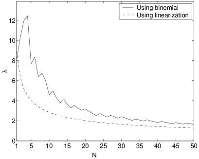
Figure 14: Graph of the smallest detectable $\lambda$ with the optimal thresholds. The dashed curve uses the linear approximation of equation (65) while the solid curve uses the binomial distribution. See text for additional discussion.

To recast the expression for $\lambda$ directly in terms of the signal amplitude, start with equation (41); $\lambda$ depends on the various pulsar parameters. The relevant quantity for the purposes of this subsection is the average of $\lambda$ over these parameters. It is quite straightforward to estimate this average. First, recall the expression for $h(t)$:

$$h(t)=F_{+}(t)A_{+}\cos\Phi(t)+F_{\times}(t)A_{\times}\sin\Phi(t)\,.$$ (69)

Since $T_{\textrm{\mbox{\tiny{coh}}}}$ is much lesser than a day (see equation (23)) we can take $F_{+\times}$ to be roughly constant. Similarly, assuming that $T_{\textrm{\mbox{\tiny{coh}}}}$ is small enough so that the pulsar signal does not shift by more than half a frequency bin, we can take the signal frequency $f(t)$ to be roughly constant. With these approximations, we get

$$\tilde{h}(f_{k})\approx\frac{T_{\textrm{\mbox{\tiny{coh}}}}}{2}(F_{+}A_{+}+F_{\times}A_{\times})\frac{\sin[\pi(f-f_{k})T_{\textrm{\mbox{\tiny{coh}}}}]}{\pi(f-f_{k})T_{\textrm{\mbox{\tiny{coh}}}}}$$ (70)

where $f$ is the instantaneous frequency of the signal and $f_{k}$ is the central Fourier frequency of the frequency bin containing $f$; $f$ is allowed to lie in the range $(f_{k}-\delta f/2,f_{k}+\delta f/2)$. Now take the square of $\tilde{h}_{k}$ and average over time to get the average non-centrality parameter for all the SFTs and note that the time averages $F_{+}^{2}$ and $F_{\times}^{2}$ are both $1/5$, and the time average of $F_{+}F_{\times}$ vanishes. Thus:

$$\lambda\approx\frac{T_{\textrm{\mbox{\tiny{coh}}}}}{10S_{n}}(A_{+}^{2}+A_{\times}^{2})\left(\frac{\sin[\pi(f-f_{k})T_{\textrm{\mbox{\tiny{coh}}}}]}{\pi(f-f_{k})T_{\textrm{\mbox{\tiny{coh}}}}}\right)^{2}\,.$$ (71)

Take the amplitudes to be of the form given in equations (7) and average over $\cos\iota\in(-1,1)$ and over the values of the signal frequency $f\in(f_{k}-\delta f/2,f_{k}+\delta f/2)$:

$$\langle\lambda\rangle_{\iota,\psi,f,\alpha,\delta} \approx \frac{4}{25}\frac{h_{0}^{2}T_{\textrm{\mbox{\tiny{coh}}}}}{S_{n}}\left(\int_{-\frac{1}{2}}^{\frac{1}{2}}\frac{\sin^{2}(\pi x)}{(\pi x)^{2}}\,dx\right)$$ (72)

$$\approx 0.7737\times\frac{4}{25}\frac{h_{0}^{2}T_{\textrm{\mbox{\tiny{coh}}}}}{S_{n}}\,.$$

We get the following value for the smallest signal that can be detected by the Hough search:

$$h_{0}=\frac{8.54}{N^{1/4}}\sqrt{\frac{S_{n}}{T_{\textrm{\mbox{\tiny{coh}}}}}}=8.54N^{1/4}\sqrt{\frac{S_{n}}{T_{\textrm{\mbox{\tiny{obs}}}}}}\,.$$ (73)

Here the second equality assumes $T_{\textrm{\mbox{\tiny{obs}}}}=NT_{\textrm{\mbox{\tiny{coh}}}}$ which be true only if the $N$ different data segments were contiguous; this is done only to compare this result with equation (74) below.

Equation (73) is the result we were looking for. This tells us that if we wish to detect a signal with a false alarm rate of $1\%$ and a false dismissal rate of $10\%$, the weakest signal that will cross the optimal thresholds is the $h_{0}$ given above. The important feature to note is that $h_{0}$ is proportional to $N^{1/4}/\sqrt{T_{\textrm{\mbox{\tiny{obs}}}}}$ while for a coherent search over the whole observation time, the sensitivity is proportional to $1/\sqrt{T_{\textrm{\mbox{\tiny{obs}}}}}$. In particular, for the same values of the false alarm and false dismissal rates as above, the sensitivity of a full coherent search directed at around a single point in parameter space is given by (see S1:pulsar ):

$$h_{0}=11.4\sqrt{\frac{S_{n}}{T_{\textrm{\mbox{\tiny{obs}}}}}}\,.$$ (74)

This illustrates the loss in sensitivity introduced by combining the different SFTs incoherently but, of course, this is compensated by the lesser computational requirements for the incoherent method. Furthermore, for say $N=2000$, the sensitivity of the Hough search is only about a factor of $4.5$ worse than a full directed coherent search.

This result helps one to make trade-offs of coherent against hierarchical searches. For example, if one is searching for a population of objects that is uniformly distributed in a plane, such as a population of young pulsars in the Galaxy, then a coherent search of any region of parameter space would go 4.5 times deeper than the incoherent method with $N=2000$. The volume of space surveyed in the plane would be $4.5^{2}=20$ times larger. However, if the incoherent method’s speed of execution allowed it to survey more than $20$ times as much parameter space (including sky area and spin-down range) then one would choose the incoherent method. This is indeed the case for pulsar searches.

Finally, equation (73) also allows us to estimate the astrophysical range of the search. Combining (9) and (73), we get:

$$d = \frac{16\pi^{2}GN^{1/4}I_{zz}\epsilon f_{r}^{2}}{8.54c^{4}}\sqrt{\frac{T_{\textrm{\mbox{\tiny{coh}}}}}{S_{n}(f_{r})}}$$

$$= 5.8\,\textrm{kpc}\times\left(\frac{N}{17000}\right)^{\frac{1}{4}}\left(\frac{I_{zz}}{10^{38}\textrm{kg-m${}^{2}$}}\right)\left(\frac{f_{r}}{500\textrm{Hz}}\right)^{2}$$

$$\times\left(\frac{\epsilon}{10^{-6}}\right)\left(\frac{T_{\textrm{\mbox{\tiny{coh}}}}}{1800\textrm{s}}\right)^{\frac{1}{2}}\left(\frac{10^{-46}\textrm{Hz}^{-1}}{S_{n}}\right)^{\frac{1}{2}}\,.$$

Here the reference values for $T_{\textrm{\mbox{\tiny{coh}}}}$ and $N$ have been chosen such that $NT_{\textrm{\mbox{\tiny{coh}}}}\approx 1$yr, and we have taken the detector sensitivity to be $10^{-23}\textrm{Hz}^{-1/2}$ at a frequency of $500$Hz, which is appropriate for the proposed advanced LIGO detector ct . A full directed coherent search does better than this by a factor of about $\sim(17000)^{1/4}\approx 12$. For the initial LIGO detector, assuming it is 10 times less sensitive than advanced LIGO, we see that it does worse than this by about a factor of $\sim 3$.

VI Hough transform with demodulated data

As equation (23) shows, using the Hough transform with SFTs as input, necessarily limits the coherent time-baseline $T_{\textrm{\mbox{\tiny{coh}}}}$, and therefore also the sensitivity of the search. To get around this limitation, we need to demodulate each coherent data segment to remove the frequency drifts caused by the Doppler modulation and the spin-down; the only limitation on $T_{\textrm{\mbox{\tiny{coh}}}}$ is then due to the available computational resources. The demodulation procedure we use is based on the $\mathcal{F}$-statistic introduced in jks . The search pipeline is very similar to the pipeline shown in figure 5, the only difference being that instead of computing the power spectrum, we calculate the $\mathcal{F}$-statistic. Subsection VI.1 provides a brief description of the $\mathcal{F}$-statistic, the master equation is derived in subsection VI.2, subsection VI.3 provides the implementation details and subsection VI.4 describes the statistics.

VI.1 The $\mathcal{F}$-statistic

Let $x(t)$ be the calibrated detector output and let $h(t)$ the waveform that we are searching for. In order to extract the signal $h(t)$ from the noise, the optimal search statistic is the likelihood function $\Lambda$ defined by

$$\ln\Lambda=(x|h)-\frac{1}{2}(h|h)$$ (76)

where the inner product $(\cdot|\cdot)$ is defined as

$$(x|y):=2\int_{0}^{\infty}\frac{\tilde{x}(f)\tilde{y}^{\star}(f)+\tilde{x}^{\star}(f)\tilde{y}(f)}{S_{n}(f)}\,\textrm{d}f\,.$$ (77)

Here, as before, $\tilde{x}(f)$ is the Fourier transform of $x(t)$ and $S_{n}(f)$ is the one-sided power spectral density. The expected waveform $h(t)$ is given by equations (6), (2) and (3). The quantity $\ln\Lambda$ is essentially the matched filter and is precisely what we should use in order to best detect the waveform $h(t)$. However, apart from the parameters $\vec{\xi}=(f_{(0)},\{f_{(n)}\},\mathbf{n})$, $\ln\Lambda$ also depends upon the other parameters such as the orientation of the pulsar, the polarization angle of the wave etc. The $\mathcal{F}$-statistic eliminates these additional variables and enables us to search over only the shape parameters $\vec{\xi}$.

Following the notation of jks , the dependence of the antenna patterns $F_{+,\times}$ on the polarization angle $\psi$ are given by

$$F_{+}(t) = \sin\zeta[a(t)\cos 2\psi+b(t)\sin 2\psi]$$ (78)

$$F_{\times}(t) = \sin\zeta[b(t)\cos 2\psi-a(t)\sin 2\psi]$$ (79)

where the functions $a(t)$ and $b(t)$ are independent of $\psi$ and $\zeta$ is the angle between the arms of the detector. If we write the phase of the gravitational wave as

$$\Phi(t)=\phi_{0}+\phi(t)\,,$$ (80)

then we can always decompose the total waveform $h(t)$ in terms of four quadratures as

$$h(t)=\sum_{i=1}^{4}A_{i}h_{i}(t)$$ (81)

where the four amplitudes $A_{i}$ are time independent and the $h_{i}$ are as follows:

$$h_{1}(t) = a(t)\cos\phi(t)\,,\qquad h_{2}(t)=b(t)\cos\phi(t)\,,$$

$$h_{3}(t) = a(t)\sin\phi(t)\,,\qquad h_{4}(t)=b(t)\sin\phi(t)\,.$$ (82)

What this decomposition achieves is a separation of the shape parameters $\vec{\xi}$ from the other pulsar parameters. The only unknown parameters in the quadratures $h_{i}$ are the shape parameters $\vec{\xi}$ while the amplitudes $A_{i}$ are independent of $\vec{\xi}$. The log likelihood function depends quadratically on the four amplitudes and we can analytically find the maximum likelihood (ML) estimators $\hat{A}_{i}$ of the amplitudes $A_{i}$ by solving the set of four coupled linear equations

$$\left.\frac{\partial\ln\Lambda}{\partial A_{i}}\right|_{A_{i}=\hat{A}_{i}}=0\,,\qquad i=1,\ldots,4\,.$$ (83)

The $\mathcal{F}$-statistic is then defined as the log likelihood ratio with the values of the amplitudes $A_{i}$ replaced by their ML estimators:

$$\mathcal{F}:=\left.\ln\Lambda\right|_{A_{i}=\hat{A}_{i}}\,.$$ (84)

The only unknown parameters in the optimal search statistic $\mathcal{F}$ are the shape parameters $\vec{\xi}$.

VI.2 The master equation

Equation (4) describes the expected time-frequency pattern when the search statistic is the Fourier transform; in other words, if the detector output $x(t)$ contains a true signal with instantaneous frequency $\hat{f}(t)$, then equation (4) tells us the value of the observed frequency $f(t)$ which would maximize $|\tilde{x}(f)|^{2}$ in the absence of noise. If we now use the $\mathcal{F}$-statistic instead of the Fourier transform, the expected time-frequency pattern is, as described below, different.

Before proceeding further, it is useful to distinguish the instantaneous frequency $f_{(0)}$ from the other shape parameters which we denote by $\vec{\lambda}$: $\vec{\xi}=(f_{(0)},\vec{\lambda})=(f_{(0)},\{f_{(n)}\},\mathbf{n})$. Let us the assume that the $\mathcal{F}$-statistic has been computed using the parameters $\vec{\lambda}_{d}$ but that the detector output consists of a signal with parameters $(f_{(0)},\vec{\lambda}$); let us denote the mismatch in the parameters by $\Delta\vec{\lambda}:=\vec{\lambda}-\vec{\lambda}_{d}$ and $\Delta f:=f-f_{(0)}$.

Since the $\mathcal{F}$-statistic is maximized when the source parameters are equal to the demodulation parameters, it is clear that if $\Delta\vec{\lambda}=0$, then the expected time-frequency pattern is just a constant frequency $f=f_{(0)}$. More generally, due to the correlations in parameter space, the mismatch $\Delta\vec{\lambda}$ may produce a residual shift in the frequency $\Delta f$. This frequency shift is determined by

$$\left.\frac{\partial\mathcal{F}(f,\vec{\lambda}_{d};f_{(0)},\vec{\lambda})}{\partial f}\right|_{\vec{\lambda}_{d},f_{(0)},\vec{\lambda}}=0\,.$$ (85)

Expand $\mathcal{F}$ in powers of $\Delta\vec{\lambda}$ and $\Delta f$ around the point $(f_{(0)},\vec{\lambda})$ up to second order (repeated indices are summed over):

$$\mathcal{F}(f,\vec{\lambda}_{d};f_{(0)},\vec{\lambda}) = \mathcal{F}(f_{(0)},\vec{\lambda})+A_{00}\left(\Delta f\right)^{2}$$

$$+ A_{0i}\Delta\lambda_{i}\Delta f+A_{ij}\Delta\lambda_{j}\Delta\lambda_{j}\,.$$

The linear terms do not appear because $\mathcal{F}$ is maximized when $\Delta f=0$ and $\Delta\vec{\lambda}=0$. With this approximation, equation (85) leads to the master equation

$$\Delta f=-\frac{A_{0i}}{2A_{00}}\Delta\lambda_{i}$$ (87)

In other words, the frequency value that maximizes the $\mathcal{F}$-statistic for a given $\Delta\vec{\lambda}$, does not correspond to the intrinsic source frequency $f_{(0)}$ but is instead given by a linear combination of the $\Delta\lambda_{i}$.

Let us rewrite equation (85) more explicitly. As shown in jks , $\mathcal{F}$ can be written in terms of the amplitude modulation functions $a(t)$ and $b(t)$ as

$$\mathcal{F}=\frac{4}{T_{\textrm{\mbox{\tiny{coh}}}}S_{n}(f_{(0)})}\frac{B|F_{a}|^{2}+A|F_{b}|^{2}-2C\mathcal{R}(F_{a}F_{b}^{\star})}{D}$$ (88)

where $A$, $B$, $C$, and $D$ are constants and

$$F_{a} = \int_{-T_{\textrm{\mbox{\tiny{coh}}}}/2}^{T_{\textrm{\mbox{\tiny{coh}}}}/2}x(t)a(t)e^{-i\Phi(t;f,\vec{\lambda}_{d})}\,dt\,,$$ (89)

$$F_{b} = \int_{-T_{\textrm{\mbox{\tiny{coh}}}}/2}^{T_{\textrm{\mbox{\tiny{coh}}}}/2}x(t)b(t)e^{-i\Phi(t;f,\vec{\lambda}_{d})}\,dt\,.$$ (90)

Since we are interested in calculating the frequency drift and not the amplitude, the variation in the phase is more important than the amplitude modulation. Thus, the factors of $a(t)$ and $b(t)$ can be taken to be constant in the above equation; see jk2 ; jk3 for a discussion of the validity of this approximation. Thus, maximizing $\mathcal{F}$ is equivalent to maximizing $|\tilde{X}(f)|^{2}$ where $\tilde{X}(f)$ is the demodulated Fourier transform (DeFT) defined as

$$\tilde{X}(f)=\int x(t)e^{-i\Phi(t;f,\vec{\lambda}_{d})}\,dt\,.$$ (91)

With this approximation, the master equation is obtained by solving

$$\left.\frac{\partial|\tilde{X}(f,\vec{\lambda}_{d};f_{(0)},\vec{\lambda})|^{2}}{\partial f}\right|_{\vec{\lambda}_{d},f_{(0)},\vec{\lambda}}=0\,.$$ (92)

The details of the calculation are given in appendix A. The result is:

$$f(t)-F_{0}(t)=\vec{\zeta}(t)\cdot({\mathbf{n}}-{\mathbf{n}}_{d})$$ (93)

where

$$F_{0}(t)=f_{(0)}+\sum_{k=1}^{s}{\Delta f_{(k)}\over k!}\left(\Delta t\right)^{k}\,,$$ (94)

and

$$\vec{\zeta}(t) = \left(F_{0}(t)+\sum_{k=1}^{s}{f_{d(k)}\over k!}\left(\Delta t\right)^{k}\right)\frac{\mathbf{v}(t)}{c}$$

$$+ \left(\sum_{k=1}^{s}{f_{d(k)}\over(k-1)!}\left(\Delta t\right)^{k-1}\right)\frac{\mathbf{r}(t)-\mathbf{r}(t_{0})}{c}\,.$$

The $\Delta f_{(k)}$’s are the residual spin-down parameters: $\Delta f_{(k)}=f_{(k)}-f_{d(k)}$, and $\mathbf{r}(t)$ is the position of the detector in the SSB frame. As expected, if $\Delta\vec{\lambda}=0$ so that $\mathbf{n}=\mathbf{n}_{d}$ and $f_{(k)}=f_{d(k)}$, then $f(t)=f_{(0)}$. Furthermore, it is clear that this master equation is qualitatively similar to equation (4) except for a constant frequency offset $\vec{\zeta}\cdot\mathbf{n}_{d}$. Thus, many of the methods obtained for the non-demodulated case will still be valid.

VI.3 Implementation details

As mentioned above, the master equations (4) and (93) are qualitatively similar except for a constant frequency offset. Thus, many of the earlier results are still valid with some minor modifications which we now explain.

Resolution in parameter space: The formula for the resolution in $f_{k}$ space is the same as given in equation (29). However, since we can make $T_{\textrm{\mbox{\tiny{coh}}}}$ much larger than before, the resolution can be made much more finer. Thus, for the first spin-down parameter, instead of equation (30), we would have

$$\delta f_{(1)}=(3.7\times 10^{-13}\textrm{Hz/s})\times\frac{365\textrm{days}}{T_{\textrm{\mbox{\tiny{obs}}}}}\cdot\frac{1\textrm{day}}{T_{\textrm{\mbox{\tiny{coh}}}}}\,.$$ (96)

Furthermore, the restriction due to the length of $T_{\textrm{\mbox{\tiny{coh}}}}$ (see equation (34)) is no longer an issue.

As for the sky-positions, using the approximation given in equation (99), the estimate of the resolution in the sky proceeds in the same way as the derivation of equation (25). The results of equations (IV.2) and (IV.2) are still valid, the only change being that $T_{\textrm{\mbox{\tiny{coh}}}}$ is now of the order of a day. Therefore, we rewrite equations (IV.2) and (IV.2) as:

$$\left(\delta\phi\right)_{\textrm{\mbox{\tiny{min}}}}=\frac{c}{v}\frac{\delta f}{\hat{f}}=\frac{c}{v\hat{f}T_{\textrm{\mbox{\tiny{coh}}}}}$$ (97)

$$=1.0\times 10^{-3}\,\textrm{rad}\times\left(\frac{1\textrm{day}}{T_{\textrm{\mbox{\tiny{coh}}}}}\right)\left(\frac{500\,\textrm{Hz}}{\hat{f}}\right)\left(\frac{10^{-4}}{v/c}\right)$$

and

$$\left(\delta\phi\right)_{\textrm{\mbox{\tiny{max}}}}=\sqrt{\frac{\delta f}{\hat{f}}\frac{c}{v}}=\sqrt{\frac{c}{v\hat{f}T_{\textrm{\mbox{\tiny{coh}}}}}}$$ (98)

$$=1.5\times 10^{-2}\,\textrm{rad}\times\left(\frac{1\textrm{day}}{T_{\textrm{\mbox{\tiny{coh}}}}}\right)^{\frac{1}{2}}\left(\frac{500\textrm{Hz}}{\hat{f}}\right)^{\frac{1}{2}}\left(\frac{10^{-4}}{v/c}\right)^{\frac{1}{2}}\,.$$

The sky resolution obtained from equation (VI.3) is therefore about 5 times better than in the non-demodulated case obtained from equation (IV.2).

Sky-patch size: Unlike in the non-demodulated case, since we are removing the frequency modulation of the signal beforehand, there is now, except for computational constraints, no restriction at all on the coherent integration time $T_{\textrm{\mbox{\tiny{coh}}}}$. Typically, $T_{\textrm{\mbox{\tiny{coh}}}}$ will be taken to be of the order of a day. However, the price we pay for this is that the demodulation is not valid for arbitrarily large patches. The patch size is determined by the largest fractional loss of sensitivity (e.g., the $\mathcal{F}$ value) we are willing to tolerate from a true signal with certain mismatch parameters $\Delta\vec{\xi}$.

If we have demodulated for a direction ${\mathbf{n}}_{d}$ in the sky, how different can ${\mathbf{n}}$ be from ${\mathbf{n}}_{d}$ so that the loss in the signal power does not become unacceptably large? In order to answer this question, we would have to analyze the parameter space metric defined in terms of the mismatch owen . The analysis of the metric will be presented elsewhere, but in this paper we shall just use a conservative estimate for the size of the sky-patch.

To estimate the size of the sky-patch, first note that the quantity $\vec{\mathbf{\zeta}}$ appearing in equation (93) is, to a very good approximation, given by

$$\vec{\mathbf{\zeta}}(t)\approx\hat{f}(t)\cdot\frac{\mathbf{v}(t)}{c}$$ (99)

where, as before, $\mathbf{v}$ is the velocity of the detector in the SSB frame. The velocity $\mathbf{v}(t)$ is the sum of two components, the velocity $\mathbf{v}_{y}$ due to the yearly motion around the sun and the velocity $\mathbf{v}_{d}$ due to the rotation of Earth around its axis: $\mathbf{v}=\mathbf{v}_{y}+\mathbf{v}_{d}$. For reference, for the GEO detector, the magnitude $v_{y}$ is about $10^{2}$ times larger than $v_{d}$. The estimate of the sky-patch size proceeds roughly like the estimate of the pixel size in equation (VI.3) except for one difference. If we take the coherent integration time $T_{\textrm{\mbox{\tiny{coh}}}}$ to be roughly of the order of less than a day, say a third of a day, then the relevant velocity is $\mathbf{v}_{d}$. Thus, the sky-patch size $h$ is roughly given by

$$h\approx\frac{c}{v_{d}}\frac{\delta f}{\hat{f}}=\frac{c}{v_{d}\hat{f}T_{\textrm{\mbox{\tiny{coh}}}}}\,.$$ (100)

Since $v_{d}$ is roughly 100 times smaller than $v$, $h\approx 100(\delta\phi)_{\textrm{\mbox{\tiny{min}}}}$. Thus, a typical sky-patch consists of about 100 pixels on a side. It should be emphasized that this is only an educated guess and is not likely to be valid for larger $T_{\textrm{\mbox{\tiny{coh}}}}$.

Validity of the look up tables: Again using the approximation given in equation (99), the number of frequency bins for which the LUT is valid can be estimated in a similar way as in the non-demodulated case. The master equation is

$$\Delta f:=f-F_{0}=\hat{f}\frac{\mathbf{v}}{c}\cdot({\mathbf{n}}-{\mathbf{n}}_{d})$$ (101)

Rewrite the equation as

$$\frac{1}{\hat{f}}=\frac{1}{\Delta f}\frac{v}{c}\cos\phi-\frac{1}{\Delta f}\frac{\mathbf{v}\cdot{\mathbf{n}}_{d}}{c}\,.$$ (102)

Keeping $\Delta f$ fixed and differentiating with respect to $\hat{f}$ leads to

$$\frac{d\hat{f}}{\hat{f}^{2}}=\frac{1}{\Delta f}\frac{v}{c}\sin\phi\,d\phi$$ (103)

As before, define $\kappa$ and $r$ by $d\hat{f}=\kappa\delta f$ and $d\phi=r\left(\delta\phi\right)_{\textrm{\mbox{\tiny{min}}}}$.

Substituting these definitions in the above equation yields

$$\kappa=\frac{rf_{0}}{\Delta f}\sin\phi$$ (104)

There are now two cases to look at, namely when $\phi$ is close to $\pi/2$ or when it is close to $0$ (or $\pi$). First the easy case when $\phi\sim\pi/2$. Here the width of the annuli is roughly the same as the pixel size: $\delta\phi\sim\left(\delta\phi\right)_{\textrm{\mbox{\tiny{min}}}}$. Thus, if $h$ is the length of a side of the sky-patch (assumed to be square) then the number of annuli in the sky patch is $h/\delta\phi$ which means $\Delta f=\delta f\cdot(h/\delta\phi)$. Substituting this in equation (104) and also setting $\phi=\pi/2$ finally leads to the result

$$\kappa=\kappa_{0}:=\frac{r}{hv/c}\,.$$ (105)

Now turn to the large annulus case. The annulus size is given by $\delta\phi\sim(\left(\delta\phi\right)_{\textrm{\mbox{\tiny{max}}}})$ and again $\Delta f=\delta f\cdot(h/\delta\phi)$. As for the numerator of equation (105), take the smallest value of $\sin\phi$, i.e. when $\phi$ is no bigger than a pixel so that $\sin\phi\sim\left(\delta\phi\right)_{\textrm{\mbox{\tiny{min}}}}$. Substituting these estimates leads to

$$\kappa=\left(\frac{r}{hv/c}\right)\sqrt{\frac{\delta f}{f_{0}}\frac{c}{v}}=\kappa_{0}\left(\delta\phi\right)_{\textrm{\mbox{\tiny{max}}}}\,.$$ (106)

From equations (VI.3) and (105) we see that typically, $\kappa$ for the thick annulus case is about 100 times smaller than for the thin annulus case.

VI.4 Statistics

This subsection describes the statistics of the Hough map, the $\mathcal{F}$-statistic, the optimal thresholds and the sensitivity. The discussion closely parallels that of section V; here we simply point out some of the differences that arise when the $\mathcal{F}$-statistic is considered instead of the normalized power.

Just as the distribution of the normalized $\rho_{k}$ power in subsection V.1 turned out to be related to the $\chi^{2}$ distribution with 2 degrees of freedom, one might intuitively expect that the distribution of $\mathcal{F}$ should also be related to a $\chi^{2}$ distribution. However, since $\mathcal{F}$ is constructed from the four filters given in equation (82), it turns out that the distribution of $2\mathcal{F}$ is a non-central $\chi^{2}$ distribution with four degrees of freedom. As before, we shall denote the non-centrality parameter by $\lambda$, and it turns out to be

$$\lambda=(h|h)$$ (107)

where the inner product $(\cdot|\cdot)$ has been defined in equation (77). A word of caution: while we use the same symbol for the non-centrality parameter as in the non-demodulated case, this definition is different from that of equation (41).

Thus, the distribution of $\mathcal{F}$ is

$$p(\mathcal{F}|\lambda) = 2\chi^{2}(2\mathcal{F}|4,\lambda)$$

$$= \left(\frac{2\mathcal{F}}{\lambda}\right)^{1/2}I_{1}(\sqrt{2\mathcal{F}\lambda})\,\exp{\left(-\mathcal{F}-\frac{\lambda}{2}\right)}$$

where $I_{1}$ is the modified Bessel function of the first order. In the absence of a signal, this reduces to

$$p(\mathcal{F}|\,0)=\mathcal{F}e^{-\mathcal{F}}\,.$$ (109)

We select frequency bins by setting a threshold $\mathcal{F}_{\textrm{\mbox{\tiny{th}}}}$ on the value of the $\mathcal{F}$-statistic in that frequency bin. Given $\mathcal{F}_{\textrm{\mbox{\tiny{th}}}}$, the probabilities for false alarm, false detection and detection are defined analogous to equations (44), (45) and (46):

$$\alpha(\mathcal{F}_{\textrm{\mbox{\tiny{th}}}}) = \int_{\mathcal{F}_{\textrm{\mbox{\tiny{th}}}}}^{\infty}p(\mathcal{F}|\,0)\,d\mathcal{F}$$ (110)

$$= (1+\mathcal{F}_{\textrm{\mbox{\tiny{th}}}})e^{-\mathcal{F}_{\textrm{\mbox{\tiny{th}}}}}\,,$$

$$\beta(\mathcal{F}_{\textrm{\mbox{\tiny{th}}}}|\lambda) = \int_{0}^{\mathcal{F}_{\textrm{\mbox{\tiny{th}}}}}p(\mathcal{F}|\lambda)\,d\mathcal{F}\,,$$ (111)

$$\eta(\mathcal{F}_{\textrm{\mbox{\tiny{th}}}}|\lambda) = \int_{\mathcal{F}_{\textrm{\mbox{\tiny{th}}}}}^{\infty}p(\mathcal{F}|\lambda)\,d\mathcal{F}\,.$$ (112)

The relation between $\alpha$ and $\mathcal{F}_{\textrm{\mbox{\tiny{th}}}}$ is different from the relation $\alpha=e^{-\rho_{\textrm{\mbox{\tiny{th}}}}}$ in the non-demodulated case. For small signals, $\eta(\mathcal{F}_{\textrm{\mbox{\tiny{th}}}}|\lambda)$ can be expanded as

$$\eta=\alpha+\frac{\lambda\mathcal{F}_{\textrm{\mbox{\tiny{th}}}}^{2}}{4}e^{-\mathcal{F}_{\textrm{\mbox{\tiny{th}}}}}+\mathcal{O}(\lambda^{2})\,.$$ (113)

Once again we will approximate this distribution by a binomial. In fact, we expect the binomial approximation to be better in this as compared to the non-demodulated search because, typically, $T_{\textrm{\mbox{\tiny{coh}}}}$ will now be larger and thus the signal will see a more representative ‘average’ of the detector antenna pattern. Finally, the expressions for the false alarm and false dismissal probabilities in the Hough plane are the same as in equations (51) and (52) but again with the $\lambda$’s and $\eta$’s as above.

With the above definitions at hand, we are now ready to optimize the thresholds $\mathcal{F}_{\textrm{\mbox{\tiny{th}}}}$ and $n_{\textrm{\mbox{\tiny{th}}}}$ using the procedure described in subsection V.2. The differences from that subsection are simply in the dependence of $\alpha$ on $\mathcal{F}_{\textrm{\mbox{\tiny{th}}}}$ and of $\eta$ on $\alpha$. The solution for $n_{\textrm{\mbox{\tiny{th}}}}$ obtained by inverting the equation $\alpha_{H}(n_{\textrm{\mbox{\tiny{th}}}},\alpha,N)$ given in figure 10 and the analytic approximation of equation (59) are unchanged. The graph of $\beta_{H}$ as a function of $\alpha$ is however, now different. The result is shown in figure 15. The optimal value for the threshold turns out to be $\mathcal{F}_{\textrm{\mbox{\tiny{th}}}}^{\star}=2.6$ corresponding to a false alarm rate of $\alpha^{\star}=0.26$. The minimum value of $\beta_{H}$ achieved by these thresholds is plotted in figure 16 as a function of $\lambda$.

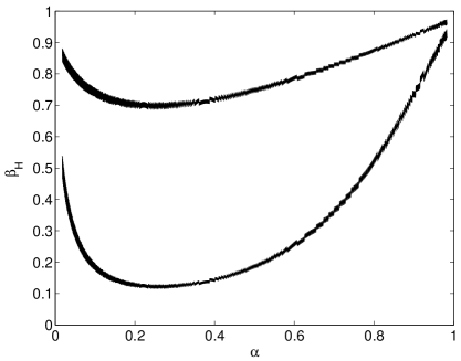
Figure 15: Graph of $\beta_{H}$ as a function of $\alpha=(1+\mathcal{F}_{\textrm{\mbox{\tiny{th}}}})e^{-\mathcal{F}_{\textrm{\mbox{\tiny{th}}}}}$ for $\lambda=0.2$ (upper curve) and $\lambda=0.4$ (lower curve). Both curves correspond to $\alpha_{H}=0.01$ and $N=1000$. The minimum of $\beta_{H}$ occurs roughly at $\alpha=0.26$ which corresponds to $\mathcal{F}_{\textrm{\mbox{\tiny{th}}}}=2.6$.

Figure 16: Graph of the minimum of $\beta_{H}$ as a function of $\lambda$ for $N=1000$ and $2000$. Both curves correspond to $\alpha_{H}=0.01$.

Finally, let us calculate the sensitivity of the search and obtain the analog of equation (73). The starting point is again equation (64) but now $\eta$ is related to $\alpha$ by equation (113) and $\alpha$ is related to $\mathcal{F}_{\textrm{\mbox{\tiny{th}}}}$ by equation (110). Then, ignoring terms of $\mathcal{O}(\lambda^{2})$ we get the linear approximation for $\beta_{H}$:

$$\beta_{H}=\frac{1}{2}\textrm{erfc}\left(-\textrm{erfc}^{-1}(2\alpha_{H}^{\star})+\frac{1}{4}\Theta e^{-\mathcal{F}_{\textrm{\mbox{\tiny{th}}}}^{\star}}(\mathcal{F}_{\textrm{\mbox{\tiny{th}}}}^{\star})^{2}\lambda\right)$$ (114)

where, as before, $\Theta$ is given by equation (66). Solving for $\lambda$ in the large $N$ limit leads to

$$\lambda\approx\frac{4\mathcal{S}}{(\mathcal{F}_{\textrm{\mbox{\tiny{th}}}}^{\star})^{2}e^{-\mathcal{F}_{\textrm{\mbox{\tiny{th}}}}^{\star}}}\sqrt{\frac{2\alpha^{\star}(1-\alpha^{\star})}{N}}\approx\frac{12.73}{\sqrt{N}}$$ (115)

where, to obtain numerical values, we have taken $\alpha_{H}^{\star}=0.01$, $\beta_{H}^{\star}=0.1$. Now average over the parameters $(\iota,\psi,\alpha,\delta)$ and obtain

$$h_{0}=\frac{8.92}{N^{1/4}}\sqrt{\frac{S_{n}}{T_{\textrm{\mbox{\tiny{coh}}}}}}=8.92\,N^{1/4}\sqrt{\frac{S_{n}}{T_{\textrm{\mbox{\tiny{obs}}}}}}\,.$$ (116)

In the second step we have assumed $T_{\textrm{\mbox{\tiny{obs}}}}=NT_{\textrm{\mbox{\tiny{coh}}}}$ which is valid only if there are no gaps in the data.

As expected, equation (116) is identical to equation (73) except for a slightly different numerical factor. Thus for comparable values of $T_{\textrm{\mbox{\tiny{coh}}}}$ and $N$, the two versions of the Hough transform search are very similar in sensitivity but the search with demodulated data does not have any restriction on $T_{\textrm{\mbox{\tiny{coh}}}}$ and will thus lead to a much greater sensitivity, though over a smaller region in parameter space. Thus, if we estimate the astrophysical range of the search as in equation (V.3), we obtain:

$$d = 15.4\,\textrm{kpc}\times\left(\frac{N}{365}\right)^{\frac{1}{4}}\left(\frac{I_{zz}}{10^{38}\textrm{kg-m${}^{2}$}}\right)\left(\frac{f_{r}}{500\textrm{Hz}}\right)^{2}$$ (117)

$$\times\left(\frac{\epsilon}{10^{-6}}\right)\left(\frac{T_{\textrm{\mbox{\tiny{coh}}}}}{1\textrm{day}}\right)^{\frac{1}{2}}\left(\frac{10^{-46}\textrm{Hz}^{-1}}{S_{n}}\right)^{\frac{1}{2}}\,.$$

Here we have taken a coherent integration time of $1$day and a total observation time of $1$yr as the reference values.

VII Conclusions

Let us summarize the main ideas and results presented in this work. Since it is not feasible to perform large parameter space searches using the matched filter with presently available computing power, we began by emphasizing the need for hierarchical searches demonstrating the need for an incoherent and computationally inexpensive search method. The Hough transform is an example of such a method. It looks for patterns in the frequency time plane by constructing a histogram in parameter space based on the consistency of observations in the time-frequency plane with an underlying model describing the pattern. We have given a general description of the Hough transform and shown its relevance for pulsar searches.

We have presented two versions of the Hough transform search. The first version takes simple Fourier transforms as input data. This restricts the time baseline of the different segments but it allows us to search over a large sky-patch. The second version takes input data which has been demodulated to remove the effects of Earth’s motion and the spin-down of the star; this is achieved by using the $\mathcal{F}$-statistic. We have presented some technical details for both flavors of the search. In particular, we show how to solve the master equation in the two cases and how the use of look-up tables can lead to a large saving in computational cost.

We have also analyzed the statistics for both cases and we saw that we need to choose two thresholds: the threshold $\rho_{\textrm{\mbox{\tiny{th}}}}$ or $\mathcal{F}_{\textrm{\mbox{\tiny{th}}}}$ on the coherent statistic used in the two cases, and the threshold $n_{\textrm{\mbox{\tiny{th}}}}$ on the number count in the Hough maps. These thresholds have been chosen in such a way that we get the lowest possible false dismissal rate for a given choice of the false alarm rate. We also estimate the sensitivity of the two flavors of the Hough transform and we find that for the same value of $T_{\textrm{\mbox{\tiny{coh}}}}$ and $N$, both variations have comparable sensitivity, which improves as $N^{-1/4}T_{\textrm{\mbox{\tiny{coh}}}}^{-1/2}$, as would be expected for an incoherent method that builds on coherent sub-steps. When compared to the sensitivity that a fully coherent search in a very large parameter space would have for the same total observation time $T_{\textrm{\mbox{\tiny{obs}}}}$, the Hough methods are worse by roughly a factor of $N^{1/4}$. Considering that the Hough transform can be expected to run very much faster than any coherent method, it should therefore be able to survey much larger volumes of space than coherent methods, despite its poorer sensitivity in any single direction. This is therefore a potentially very important method for conducting large-scale gravitational wave pulsar surveys.

Appendix A The master equation for the search with demodulated data

Here we detail the steps leading from equation (92) to the master equation (93).

Ignoring the amplitude modulation and a possible constant phase, the signal from a pulsar with parameters $(f_{(0)};\vec{\lambda})=(f_{(0)};{\mathbf{n}},\{f_{(n)}\})$ would be:

$$h(t,f_{(0)},\vec{\lambda})=e^{i\Phi(t,f_{(0)},\vec{\lambda})}\,,$$ (118)

where

$$\Phi(t;f_{(0)},\vec{\lambda})=2\pi\left[f_{(0)}\Delta t_{\bf n}+\sum_{k=1}^{s}{f_{(k)}\over(k+1)!}\left(\Delta t_{\bf n}\right)^{k+1}\right]\,,$$ (119)

and

$$\Delta t_{\bf n}=t_{\textrm{\mbox{\tiny{ssb}}}}(t,{\bf n})-t_{\textrm{\mbox{\tiny{ssb}}}}(t_{0},{\bf n})\,.$$ (120)

Here $t_{0}$ is the time in the detector frame to which the frequency and spin-down parameters refer to and $t_{\textrm{\mbox{\tiny{ssb}}}}$ is time in the SSB frame. Neglecting higher order relativistic effects, the detector time $t$ is related to $t_{\textrm{\mbox{\tiny{ssb}}}}$ by

$$t_{\textrm{\mbox{\tiny{ssb}}}}(t,{\mathbf{n}})=t+\frac{\mathbf{r}(t)\cdot\mathbf{{n}}}{c}$$ (121)

where $\mathbf{r}(t)$ is the detector position in the SSB frame.

The DeFT of the pulsar signal (118) with respect to the demodulation parameters $(f,\vec{\lambda}_{d})$ is:

$$\tilde{X}(f)=\int_{-\frac{1}{2}T_{\textrm{\mbox{\tiny{coh}}}}}^{\frac{1}{2}T_{\textrm{\mbox{\tiny{coh}}}}}e^{i[\Phi(t,f_{(0)},\vec{\lambda})-\Phi(t,f,\vec{\lambda}_{d})]}dt\,.$$ (122)

Without any loss of generality, we have taken the coherent time interval to be centered around $t=0$ so that the integral is from $-T_{\textrm{\mbox{\tiny{coh}}}}/2$ to $T_{\textrm{\mbox{\tiny{coh}}}}/2$.

Our goal is to determine an analytical expression for the value of $f$ that maximizes the power $P(f)=|\tilde{X}(f)|^{2}$ in terms of $f_{(0)}$, $\vec{\lambda}_{d}$ and $\Delta\vec{\lambda}$. To do this, first expand $\Delta\Phi(t):=\Phi(t,f_{(0)},\vec{\lambda})-\Phi(t,f,\vec{\lambda}_{d})$ in powers of $\Delta f_{(k)}:=f_{(k)}-f_{d(k)}$ and $\Delta\mathbf{n}:=\mathbf{n}-\mathbf{n}_{d}$, keeping only terms up to linear order:

$$\frac{\Delta\Phi(t)}{2\pi}\approx\left(f_{(0)}-f\right){\Delta t_{{\mathbf{n}}_{d}}}+\sum_{k=1}^{s}{\Delta f_{(k)}\over(k+1)!}\left({\Delta t_{{\mathbf{n}}_{d}}}\right)^{k+1}$$

$$+\left[f_{(0)}+\sum_{k=1}^{s}\frac{f_{(k)}}{k!}\left(\Delta t_{{\mathbf{n}}_{d}}\right)^{k}\right]\frac{\Delta\mathbf{r}}{c}\cdot\Delta\mathbf{n}$$ (123)

where $\Delta\mathbf{r}=\mathbf{r}(t)-\mathbf{r}(t_{0})$.

Now Taylor expand $\Delta\Phi(t)$ about a fiducial time $t_{1}$ in the interval $-T_{\textrm{\mbox{\tiny{coh}}}}/2\leq t_{1}\leq T_{\textrm{\mbox{\tiny{coh}}}}/2$ again retaining terms only up to linear order

$$\tilde{X}(f) \approx \int_{-\frac{1}{2}T_{\textrm{\mbox{\tiny{coh}}}}}^{\frac{1}{2}T_{\textrm{\mbox{\tiny{coh}}}}}e^{i\left(\Delta\Phi(t_{1})+(t-t_{1}){\displaystyle\partial\Delta\Phi\over\displaystyle\partial t}\right)}dt$$ (124)

$$= e^{i\Delta\Phi(t_{1})}\int_{-\frac{1}{2}T_{\textrm{\mbox{\tiny{coh}}}}}^{\frac{1}{2}T_{\textrm{\mbox{\tiny{coh}}}}}e^{i(t-t_{1}){\displaystyle\partial\Delta\Phi\over\displaystyle\partial t}}dt\ .$$

$P(f)$ does not depend on $\Delta\Phi(t_{1})$, and its maximum is reached for the value of $f$ that satisfies

$$\left.\frac{\partial\Delta\Phi}{\partial t}\right|_{t=t_{1}}=0\,.$$ (125)

Differentiating (123) with respect to $t$, we get

$${\frac{1}{2\pi}}\left.\frac{\partial\Delta\Phi}{\partial t}\right|_{t=t_{1}}$$ (126)

$$\approx\left(f_{(0)}-f+\sum_{k=1}^{s}{\Delta f_{(k)}\over k!}\left(\Delta t_{1}\right)^{k}\right)\left(1+{{\mathbf{v}}(t_{1})\over c}\cdot{\mathbf{n}}_{d}\right)$$

$$+\left(f_{(0)}+\sum_{k=1}^{s}\frac{f_{(k)}}{k!}\left(\Delta t_{1}\right)^{k}\right){{\mathbf{v}}(t_{1})\over c}\cdot\Delta\mathbf{n}$$

$$+\left(\sum_{k=1}^{s}\frac{f_{(k)}}{(k-1)!}\left(\Delta t_{1}\right)^{k-1}\right)\left(1+{{\mathbf{v}}(t_{1})\over c}\cdot{\mathbf{n}}_{d}\right)\frac{\Delta\mathbf{r}_{1}}{c}\cdot\Delta\mathbf{n}$$

where $\Delta t_{1}=t_{\textrm{\mbox{\tiny{ssb}}}}(t_{1},{\mathbf{n}}_{d})-t_{\textrm{\mbox{\tiny{ssb}}}}(t_{0},{\mathbf{n}}_{d})$ and $\Delta\mathbf{r}_{1}=\mathbf{r}(t_{1})-\mathbf{r}(t_{0})$. Setting the right hand side of this equation to zero and dropping higher order terms leads to

$$f-F_{0}=\left(F_{0}+\sum_{k=1}^{s}{f_{d(k)}\over k!}\left(\Delta t_{1}\right)^{k}\right){{\mathbf{v}}(t_{1})\over c}\cdot\Delta\mathbf{n}$$

$$+\left(\sum_{k=1}^{s}{{f_{d(k)}}\over(k-1)!}\left(\Delta t_{1}\right)^{k-1}\right)\frac{\Delta\mathbf{r}_{1}}{c}\cdot\Delta\mathbf{n}$$ (127)

where $F_{0}$ is as given in equation (94). All the dependence on the residual spin-down parameters appears only in the definition of $F_{0}$ and, after replacing the arbitrary time $t_{1}$ by $t$, we get equation (93).

References

- (1) B. Abbott et.al. (The LIGO Scientific Collaboration), Nucl. Instrum. Meth. A517, 154 (2004).
- (2) A. Abramovici et al., Science 256, 325 (1992).
- (3) B. Barish and R. Weiss, Phys. Today 52, No. 10, 44 (1999).
- (4) B. Willke et al., Class. Quant. Grav., 19(7), 1377 (2002).
- (5) S. Goßler et al., Class. Quant. Grav., 19(7), 1835 (2002).
- (6) B. Abbott et al. (The LIGO Scientific Collaboration), Phys. Rev. D69, 082004 (2004).
- (7) P. Jaranowski, A. Królak, and B.F. Schutz, Phys. Rev. D58 (1998) 063001.
- (8) P.R. Brady, T. Creighton, C. Cutler, and B.F. Schutz, Phys. Rev. D57 (1998) 2101-2116.
- (9) P.R. Brady and T. Creighton, Phys. Rev. D61 (2000) 082001.
- (10) A.J. Storkey, N.C. Hambly, C.K.I. Williams, and R.G. Mann, Mon. Not. Roy. Astron. Soc. 347 36-51 (2004) (astro-ph/0309565).
- (11) P. Ballester, In Astronomical Data Analysis Software and Systems III, ASP Conference Series, Vol. 61, p. 319 (1994), Edts. D.R. Crabtree, R.J. Hanisch, J. Barnes, Astronomical Society of the Pacific.
- (12) C. Aulbert, In preparation.
- (13) J. Illingworth and J. Kittler, Computer Vision, Graphics, and Image Processing 44, 87-116 (1988)
- (14) P.V.C. Hough, In International Conference on High Energy Accelerators and Instrumentation, CERN (1959).
- (15) P.V.C. Hough, U. S. Patent 3,069,654, 1962.
- (16) http://www.lsc-group.phys.uwm.edu/lal/.
- (17) C. Bradaschia et al., Nucl. Instrum. Methods A 289, 518 (1990).
- (18) B. Caron et al., Nucl. Phys. B-Proc. Suppl., 54, 167 (1994).
- (19) S. Frasca and C La Posta, Il Nuovo Cimento 14 C, 235 (1991).
- (20) B.F. Schutz and M.A. Papa, Proceedings of January 1999 Moriond meeting “Gravitational Waves and Experimental Gravity” (gr-qc/9905018).
- (21) M.A. Papa, B.F. Schutz, and A.M. Sintes, ICTP Lecture Notes Series, Volume III (ISBN 92-95003-05-5), p. 431-442 (2001), Italy, Edts. V. Ferrari, J.C. Miller, L. Rezzolla (gr-qc/0011034).
- (22) L. Brocco, S. Frasca, C. Palomba and F. Ricci, Class. Quant. Grav. 20 S655-S664 (2003).
- (23) P. Astone, S. Frasca, and M.A. Papa, In Proc. of the Aspen Winter Conference on Gravitational Waves and their Detection, ed. by S.Meshkov, 1997.
- (24) S. Frasca, Int.J. of Mod. Phys. D 9 369 (2000).
- (25) V.M. Kaspi, J.H. Taylor, and M.F. Ryba, ApJ 428, 713 (1994).
- (26) C. Cutler, I. Gholami, and B. Krishnan, In preparation.
- (27) B. Allen, M.A. Papa, and B.F. Schutz, Phys. Rev. D 66, 102003 (2002).
- (28) B. Owen, Phys. Rev. D53, 6749 (1996).
- (29) C. Cutler and K. S. Thorne, In Proceedings of International Conference on General Relativity & Gravitation, ed. by NT Bishop and SD Maharaj, World Scientific, 2002 (gr-qc/0204090).
- (30) P. Jaranowski and A. Królak, Phys.Rev. D59, 063003 (1999).
- (31) P. Jaranowski and A. Królak, Phys.Rev. D61, 062001 (2000).