The discrete energy method in numerical relativity: Towards long-term stability

Abstract

The energy method can be used to identify well-posed initial boundary value problems for quasi-linear, symmetric hyperbolic partial differential equations with maximally dissipative boundary conditions. A similar analysis of the discrete system can be used to construct stable finite difference equations for these problems at the linear level. In this paper we apply these techniques to some test problems commonly used in numerical relativity and observe that while we obtain convergent schemes, fast growing modes, or “artificial instabilities,” contaminate the solution. We find that these growing modes can partially arise from the lack of a Leibnitz rule for discrete derivatives and discuss ways to limit this spurious growth.

I Introduction

Einstein’s theory of general relativity is described by a complicated set of coupled, nonlinear partial differential equations. Like the Maxwell equations of classical electromagnetism, the Einstein equations are over-determined, and can be separated into hyperbolic evolution and elliptic constraint equations, as in the Arnowitt–Deser–Misner (ADM) decomposition ADM . The complexity of these equations is such that analytic solutions have been found for only very special configurations, and numerical studies arguably provide the only means to explore a wide variety of astrophysical and theoretically significant problems lehnerreview ; shapirobaumgarte . Unfortunately, these numerical solutions are often prone to various instabilities, which we divide into three classes: (1) continuum instabilities, (2) numerical instabilities and (3) artificial long-term “instabilities” (ALTI).

Continuum instabilities exist in the formulation of the continuum problem (and thus are naturally reflected in any consistent numerical scheme), and are characterized by the solution itself or some perturbation of it either “blowing up” at a finite time or growing fast in time. These instabilities may reflect physical phenomena, such as turbulence in fluids or the threshold of black hole formation gundlach , or may be an artifact of the formulation of the problem. For instance, ill-posed problems suffer from these instabilities, which also manifest themselves as numerical ones (see  gko , and convergence for an illustration in numerical relativity). Numerical instabilities are characterized by errors that, at a fixed time, increase as the discretization scale is decreased. These instabilities are present in many discretization schemes for well-posed problems that appear “natural”, such as the forward-time, centered-space scheme for the advection equation. Finally, ALTI are sometimes exhibited even by numerically stable implementations, whenever errors grow too fast for the desired simulation time-scale and available computational resources. Although these may not be instabilities in the strict sense, given that –as defined here– they are not present at the continuum and do go away with resolution, they are problematic in practice as they limit the time-length of a reliable simulation. In this paper we focus on this long-term error growth together with the application of the techniques described in paper1 , which throughout this work we refer to as Paper I.

The stability of finite difference approximations (FDAs) for simple Initial Value Problems (IVP) with constant coefficients and periodic boundaries is often analyzed in discrete Fourier space, by examining the norm of the amplification matrix. This method, however, does not generalize in a straightforward way to more complicated problems, such as those with variable coefficients or those with boundaries. A more powerful technique is based on the energy method gko , also used to identify well-posed continuum problems. This method can be used in all problems for which the continuum energy method applies, e.g., quasi-linear parabolic and symmetric hyperbolic partial differential equations with appropriate boundary conditions. The discrete formulation reproduces the continuum analysis, including the calculation of a discrete energy estimate, which can be used to meet sufficient conditions for a stable numerical method. Combining these estimates with the consistency of the discrete system with the continuum problem, stability of the linear problem is equivalent to convergence via the Lax equivalence theorem Lax . While our focus in general relativity is on the nonlinear Einstein equations, stability of the linearized equations is obviously a necessary step for solving non-linear problems, in particular those with smooth solutions. In the absence of matter, smooth solutions are indeed expected in general relativity when appropriate slicing conditions are used hyp .

As described in Paper I, a discrete energy estimate can be obtained when using finite difference operators that satisfy summation by parts (SBP) kreiss-scherer , a discrete version of integration by parts, as well as appropriate boundary conditions olsson and time integrators kreiss-wu ; tadmor . Paper I presents and extends these techniques in the context of numerical relativity. In this paper we demonstrate these techniques using some common test problems employed in the field. We evolve Klein–Gordon scalar fields and Maxwell fields on fixed Schwarzschild spacetimes. We also consider gauge wave spacetimes, obtained via coordinate transformations of flat spacetime. We show that we naturally obtain stable and convergent numerical schemes by construction, even when an inner boundary is used to remove the black hole singularity (black hole excision) unruh .

A second goal of this paper is to understand some causes of long-term error growth (ALTI), and ways of eliminating or minimizing it by achieving strict stability olsson . Numerical solutions of the Einstein equations are frequently plagued by such long-term errors. Since at least some of these appear in numerically stable implementations, their cause is often attributed to the formulation of the equations. While this may be the case in a number of problems, as discussed below, some numerical experiments of simple differential equations with no continuum instabilities also display this same artificial long-term instability —even when discretized in a numerically stable way—. Hence, it is important to devise numerical techniques to control this spurious growth in the numerical error. We find that this spurious error growth is allowed in the absence of sharp energy estimates for the discrete problem. This can arise, from among other reasons, because the discrete derivatives fail to satisfy the Leibnitz Rule. With this observation in mind, we discuss here a method to remedy some of these problems by constructing schemes that suppress excitations of ALTI.

This work is organized as follows: We first summarize, in Section II, some results from Paper I, in order to introduce some notation. Section III discusses the notion of strict stability, and we present simple examples of “natural” schemes that are numerically stable but not strictly stable, for which the errors grow fast in time. We then explain the basic strategy to achieve strict stability, and show how this eliminates ALTI. In Section IV we present some test problems from numerical relativity: three-dimensional scalar and electromagnetic fields propagating on a fixed Schwarzschild black hole geometry, and one-dimensional perturbations of a dynamical slicing of flat spacetime (“gauge wave”). The first cases allow us to test black hole excision, while the gauge wave has a time dependent background without a sharp energy estimate. However, a sharp energy estimate does exist for the subsidiary constraint system, and it can be used to understand the nature of the ALTI and suppress them. Although more work would need to be done, these observations and ideas could be useful when evolving Einstein’s equations in more complicated situations. In Section V we present numerical simulations of the systems discussed in Section IV. Finally, in appendix A we discuss cubical excision boundaries for black hole spacetimes.

II Numerical stability and the energy method: an overview

We first review the construction of numerically stable finite-difference schemes using the discrete energy method for linear, symmetric hyperbolic initial-boundary value problems (IBVPs) with maximally dissipative boundary conditions. While the discussion here is brief, further information can be found in the standard text by Gustaffsson, Kreiss, and Oliger gko , works by Olsson olsson , and Paper I, for their particular application in numerical relativity. Sufficient conditions for a stable discretization are fulfilled when:

1. The continuum problem can be shown to be well posed using the energy method.

2. Spatial difference operators that satisfy SBP on the computational domain are used.

3. Boundary conditions are imposed via orthogonal projections olsson .

4. The semi-discrete equations are integrated with a locally stable time integrator, e.g., third or fourth order Runge–Kutta kreiss-wu ; tadmor .

5. Optionally, explicit dissipation may be added using operators that do not spoil the energy estimates, and different ways of writing the discrete equations may be explored to achieve strict stability.

As an example, consider a set of linear, symmetric hyperbolic equations on a one-dimensional domain, $x\in[a,b]$. This domain is discretized with points $x_{i}=a+i\Delta x$, $i=0\ldots N$, where $\Delta x=(b-a)/N$, and a discrete scalar product,

$$(u,v):=\Delta x\sum_{i,j=0}^{N}\sigma_{ij}u_{i}v_{j}\,,$$ (1)

is introduced for some positive definite matrix with elements $\sigma_{ij}$. In the limit $\Delta x\to 0$ this scalar product approaches the continuum one given by

$$\langle u,v\rangle:=\int_{a}^{b}uv\,dx\,.$$ (2)

The standard continuum derivative operators and scalar products satisfy integration by parts:

$$\langle u^{\prime},v\rangle+\langle u,v^{\prime}\rangle=uv|_{a}^{b}.$$ (3)

Similarly, a discrete difference operator $D$ is said to satisfy SBP, if there is a scalar product with respect to which

$$(Du,v)+(u,Dv)=uv|_{a}^{b}$$ (4)

holds. The simplest difference operator and scalar product that satisfy SBP on this domain are

$$\begin{array}[]{lll}D=D_{+}\,,&\sigma_{00}=\frac{1}{2}&\mbox{ for }i=0\\ D=D_{0}\,,&\sigma_{ii}=1&\mbox{ for }i=1\ldots N-1\\ D=D_{-}\,,&\sigma_{NN}=\frac{1}{2}&\mbox{ for }i=N\end{array}$$ (5)

where $D_{0}u=(u_{i+1}-u_{i-1})/(2\Delta x)$, $D_{-}u=(u_{i}-u_{i-1})/\Delta x$, $D_{+}u=(u_{i+1}-u_{i})/\Delta x$, and the scalar product is diagonal: $\sigma_{ij}=0$ for $i\neq j$. Higher order operators satisfying SBP have been constructed by Strand strand . Domains with inner boundaries in several dimensions introduce additional complexities, and we refer the reader to Paper I for more information.

We sometimes use explicit numerical dissipation. For that purpose we modify near boundaries the standard Kreiss–Oliger dissipative operator for second order derivatives, $Q_{d}$, so that it does not spoil the semi-discrete estimate, i.e., so that it satisfies $(u,Q_{d}u)\leq 0$. The operator $Q_{d}$, which is fully described in Paper I, is added to the right-hand side of the evolution equations. In the absence of inner boundaries, it is (on each direction)

$$Q_{d}u_{0} = -2\epsilon\Delta xD_{+}^{2}u_{0},$$

$$Q_{d}u_{1} = -\epsilon\Delta x(D_{+}^{2}-2D_{+}D_{-})u_{1},$$

$$Q_{d}u_{i} = -\epsilon(\Delta x)^{3}(D_{+}D_{-})^{2}u_{i},\;\mbox{ for }i=2,\ldots,N-2$$

$$Q_{d}u_{N-1} = -\epsilon\Delta x(D_{-}^{2}-2D_{+}D_{-})u_{N-1},$$

$$Q_{d}u_{N} = -2\epsilon\Delta xD_{-}^{2}u_{N}.$$ (6)

We discretize the equations in time using the method of lines, and use third-order Runge–Kutta to integrate the equations. More precisely, for the ordinary differential system

$$\frac{\partial u}{\partial t}=L(t,\,u),$$

we integrate the solution $u^{n}$, defined at time $t^{n}$, to the advanced time, $t^{n+1}=t^{n}+\Delta t$, obtaining $u^{n+1}$, through

$$u^{(1)} = u^{n}+\frac{1}{2}\Delta t\,k_{1},$$

$$u^{(2)} = u^{n}+\frac{3}{4}\Delta t\,k_{2},$$

$$u^{n+1} = u^{n}+\frac{1}{9}\Delta t\,(2k_{1}+3k_{2}+4k_{3}),$$ (7)

where

$$k_{1} = L\left(t^{n},\,u^{n}\right),$$

$$k_{2} = L\left(t^{n}+\frac{1}{2}\Delta t,\,u^{(1)}\right),$$

$$k_{3} = L\left(t^{n}+\frac{3}{4}\Delta t,\,u^{(2)}\right).$$ (8)

III Artificial long-term instabilities and strict stability

Throughout this paper we call artificial long-term instabilities (ALTI) those instabilities that are neither numerical—the errors at a fixed time do not become larger when the resolution is increased, but rather converge to zero—nor true instabilities of the continuous solution. These instabilities, as shown in some examples below, can appear quite generically in long-term simulations.

There are least two possible ways to suppress ALTI’s:

1. Constructing strictly stable discretizations with respect to a conveniently defined energy. The equations are written such that a sharp continuum estimate also holds for the semi-discrete equations. The semi-discrete energy will then closely mirror the continuum energy estimate.

2. Explicit numerical dissipation can be used to eliminate high frequency errors, shifting the spectrum of the amplification matrix.

Although the latter solution is easy to implement, it may not be effective if the ALTI excites low frequency modes. The first solution, on the other hand, does not introduce artificial damping, but such a discretization may be difficult or even impossible to find for generic systems of equations. For example, no general sharp estimate for the full Einstein equations is known at this time. Thus, these two possibilities can be seen as complementary to each other.

The energy of a solution, $u$, of a set of linear partial differential equations is defined as

$${\cal E}(t)=\langle u,Hu\rangle\;,$$ (9)

where $H$ is a positive definite symmetrizer for the system. This energy is not unique, reflecting the freedom in choosing the symmetrizer, $H$. The energy method provides an estimate for the growth rate of the energy in the form of an inequality, say,

$$\frac{d{\mathcal{E}}}{dt}\leq F({\mathcal{E}})\,.$$ (10)

and thus provides a bound to the energy growth. This bound may be much larger than the actual growth rate for the continuum solution, in which case we say that the energy estimate is coarse. When the estimate is close to the actual energy growth rate of a solution, the estimate is sharp. While the behavior of the continuum solution is independent of a particular bound, as we discuss in this paper, numerical solutions sometimes do have a large growth if this is allowed. Thus, the sharper the bound is, the smaller the possible spurious growth in the numerical solution.

Finding a sharp estimate is problem-dependent, and the definition of a convenient energy has to be analyzed on each case. One usually attempts to find a sharp energy bound by exploiting the freedom in choosing the symmetrizer. For example, a well-defined local physical energy exists in many physically motivated problems, which can be used to select a preferred symmetrizer. The evolution equations must be written such that they are symmetrizable with respect to this energy, but this is in general possible. Although a locally positive definite energy for the Einstein equations does not exist, relatively sharp estimates exist for some problems friedichstablemink ; chrisklain ; rodklain .

The energy method can be used to derive discrete estimates. Using difference operators that satisfy SBP and representing the boundary conditions through orthogonal projections, the semi-discrete calculation mirrors the continuum analysis. When a discrete energy estimate is present, the discrete system is numerically stable by construction. A discrete system with the same energy estimate as the continuum problem may be defined as strictly stable. However, we are particularly interested in systems for which the energy estimate is sharp, and we therefore reserve the term strictly stable for discrete systems that match a sharp continuum energy estimate.

Assuming a sharp energy estimate exists for the continuum problem, in this paper we consider how the discrete problem might be implemented to preserve this sharp estimate at the numerical level. This can be exploited to achieve long-term stability in an otherwise numerically stable but long-term unstable scheme. Throughout this paper we only use numerically stable schemes, even when not explicitly mentioned. Therefore, we concentrate on their long-term stability.

Finally, we note that the sharp energy estimates discussed here are for semi-discrete systems, where time is continuous but space has been discretized. A sharp estimate may, in principle, be lost owing to error introduced by the temporal integration . The experiments presented in this paper and in hyperGR suggest that (at least in the cases considered) if strict stability is lost, the effects are not serious. The semi-discrete analysis appears to adequately represent the fully discrete simulation.

III.1 Example 1: A simple model

Consider the initial-boundary value problem defined by the equation

$$\dot{u}=u^{\prime}+u/x\;,\qquad x\in[1,2],\qquad t\geq 0\;,$$ (11)

together with some initial data and maximally dissipative boundary conditions. Let us consider the numerically stable discretization defined by

$$\dot{u}_{i}=Du_{i}+u_{i}/x_{i}\;\;\;,\;\;\;i=0\ldots N,\qquad t\geq 0\;,$$ (12)

with the discrete derivative, $D$, given by Eq. (5), third-order Runge–Kutta for the time integration [cf. Eq. (7)], and maximally dissipative boundary conditions imposed through orthogonal projections. Figure 1 shows results from simulations using this numerical scheme and $u(t=0,x)=1/x$ as initial data and $u(t,2)=1/2$ as boundary conditions, which corresponds to the time-independent solution $u(t,x)=1/x$ . The figure plots the $L_{2}$ norm of the errors with respect to the exact solution as a function of time, at different resolutions (obtained on uniform grids, where the number of points ranges from $81$ to $5121$). At a fixed time, the errors decrease with resolution, verifying that, as expected, the scheme is numerically stable. At fixed resolution, however, the error grows as a function of time, i.e., the solution has long-term error growth, or ALTI.

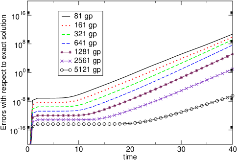
Figure 1: This figure shows the $L_{2}$ norm of the solution error for Eq. (12) as a function of time at many different discretization scales, with initial data $u(0,x)=1/x$ and boundary conditions $u(t,2)=1/2$. The solution is calculated with a numerically stable discretization that is not strictly stable. Although convergent, the error in the solution clearly displays an exponential growth. The CFL factor used is 0.8.

.

To understand this behavior we examine an energy norm of the solution. Let the continuum energy be (using $H=1$)

$${\cal E}^{(1)}=\langle u,u\rangle\;,$$ (13)

We obtain an energy estimate by taking a time derivative in both sides of Eq. (13) and using the evolution equation (11), obtaining

$$\dot{{\cal E}}^{(1)} = \langle\dot{u},u\rangle+\langle u,\dot{u}\rangle$$ (14)

$$= \langle u^{\prime}+u/x,u\rangle+\langle u,u^{\prime}+u/x\rangle$$

$$= \langle u^{\prime},u\rangle+\langle u,u^{\prime}\rangle+\langle u/x,u\rangle+\langle u,u/x\rangle$$

$$= -u(a)^{2}+u(b)^{2}+\langle u/x,u\rangle+\langle u,u/x\rangle$$

$$= -u(a)^{2}+\frac{1}{4}+2\langle u/x,u\rangle$$

$$\leq \frac{1}{4}+2\langle u/x,u\rangle$$

$$\leq \frac{1}{4}+2a^{-1}\langle u,u\rangle$$

That is,

$$\dot{{\cal E}}^{(1)}\leq\frac{1}{4}+2a^{-1}{\cal E}^{(1)}\;.$$ (16)

Only integration by parts was used to derive this estimate, between Eqs. (14) and (III.1).

Now consider the discrete problem. We define a semi-discrete energy analogous to that one defined in Eq. (13), namely

$$E^{(1)}=(u,u)\;.$$ (17)

The derivation of the above continuum energy estimate can be repeated at the semidiscrete level, provided the difference operator satisfies SBP, since only integration by parts was used at the continuum. Therefore, the same estimate holds for the semi-discrete energy defined in Eq. (17). That is,

$$\dot{E}^{(1)}\leq\frac{1}{4}+2a^{-1}E^{(1)}\;.$$ (18)

The continuum estimate, Eq. (16), and the semi-discrete counterpart, Eq. (18), guarantee that the norm of the continuum and numerical solutions will grow with a rate bounded by $e^{2t/a}$. As these are estimates, this does not mean that the exponential growth actually occurs. Indeed, the continuum solution does not grow, since Eq. (11) is the advection equation with the time-independent change of variables, $v=xu$. With this transformation, Eq. (11) becomes $\dot{v}=v^{\prime}$. However, the results shown in Fig. 1 indicate that an exponential growth does appear in the numerical solution.

We now define a new energy , that allows for a sharper energy estimate and, consequently, a better discrete system. Let this new energy (defined with $H=x^{2}$) be

$${\cal E}^{(2)}=\frac{1}{2}\langle u,x^{2}u\rangle\;.$$ (19)

As before, an estimate is obtained by differentiating in time, substituting in the evolution equations, and using integration by parts to get

$$\dot{{\cal E}}^{(2)} = \int_{a}^{b}x^{2}u\dot{u}\,dx=\int_{a}^{b}x^{2}u\left(u^{\prime}+\frac{u}{x}\right)dx$$ (20)

$$= \int_{a}^{b}\left(\frac{x^{2}u^{2}}{2}\right)^{\prime}dx=-\frac{a^{2}u(a)^{2}}{2}\leq 0\;.$$

In deriving the estimate (20) we have used the Leibnitz rule, in the third equality. The analogous semi-discrete energy is now

$$E^{(2)}=\frac{1}{2}(u,x^{2}u)\;.$$ (21)

However this semi-discrete energy will not, in general, satisfy a discrete version of the continuum estimate given in (20). The reason is that although $D$ satisfies SBP, it does not generally satisfy the Leibnitz rule, which was necessary in deriving the estimate (20). It can actually be checked that, because of this, discretizing the system as in Eq. (12) will not reproduce the continuum estimate, i.e.

$$\dot{E}^{(2)}\neq-\frac{a^{2}u(a)^{2}}{2}.$$ (22)

An alternative is to rewrite the evolution equation (11) such that the Leibnitz rule is unnecessary to obtain the continuum estimate, Eq. (20). Then a semi-discrete version of this estimate does hold if the difference operator satisfies SBP. To do so we write Eq. (11) as

$$\dot{u}=\frac{1}{x}(ux)^{\prime}\;.$$ (23)

This gives the same estimate as before:

$$\dot{{\cal E}}^{(2)}=\int_{a}^{b}x^{2}u\dot{u}\,dx=\int_{a}^{b}xu(xu)^{\prime}\,dx=-\frac{1}{2}\left[au(a)\right]^{2}\leq 0.$$ (24)

However, in deriving the estimate (24) we have only used integration by parts, and not the Leibnitz rule. Therefore, the semi-discrete energy estimate

$$\dot{E}^{(2)}=-\frac{a^{2}u(a)^{2}}{2}.$$ (25)

follows immediately if the semidiscrete equation is written as

$$\dot{u}=\frac{1}{x}D(ux).$$ (26)

and $D$ satisfies SBP.

Figure 2 shows numerical results obtained by evolving Eq. (11) using two discretizations, given by Eqs. (12,26). Eqs. (11) and (23) are equivalent, they have the same set of solutions. However, their discrete counterparts, Eqs. (12) and (26), do not have the same solutions at fixed resolution. In one case the solution error grows as a function of time, in the other case it does not.

It is experimentally found that in this example (and others discussed below) the growing numerical error in the non-strictly stable discretization is manifest in high frequency modes, which can be eliminated by adding a small amount of dissipation, as is also shown in Figure 2.

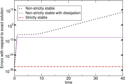
Figure 2: This figure compares the solution error, at fixed resolution, for different discretizations of Eq. (11). The dotted line shows the one of the lines of Fig.1, i.e., the $L_{2}$ norm of the error for a non-strictly stable discretization, given by Eq. (12). The solid line shows the error for the same simulation with some numerical dissipation ($\sigma=0.01$). The dashed line, in turn, shows the error for the (non-dissipative) strictly stable discretization given by Eq. (26). In all these runs $\Delta x=1/80$ and CFL=0.8. Even though both the strictly stable and the non-strictly but dissipative schemes give long term stability, the former discretization is much more accurate.

III.2 Example 2: Energy preserving and non-preserving system

Consider now an equation with variable-coefficients in the principal part and a lower order term that in principle allows for energy growth,

$$\dot{u}=2cu^{\prime}+uc^{\prime}+F(u),$$ (27)

defined on a compact domain $x\in[a,b]$. For simplicity we assume that $c=c(x)>0$, and define the energy ${\cal E}=\langle u,u\rangle/2$. Homogeneous boundary conditions are given at $x=b$. Rewriting the equation as $\dot{u}=(uc)^{\prime}+cu^{\prime}+F(u)$, one can easily show, using only integration by parts, that the estimate

$$\dot{{\cal E}}=(u^{2}c)|^{b}_{a}+\langle F,u\rangle=-u(a)^{2}c(a)+\langle F,u\rangle\leq\langle F,u\rangle$$

holds. Therefore, writing the semi-discrete equation as

$$\dot{u}=D(uc)+cDu+F(u)$$ (28)

gives the same semi-discrete energy estimate,

$$\dot{E}\leq(F,u)$$

If $F=0$ then $\dot{E},\dot{{\cal E}}\leq 0$ and the continuum and discrete solutions cannot grow in time. Equations with features similar to those of Eq.(27) with $F=0$ appear in the Klein–Gordon and Maxwell fields on fixed black hole backgrounds, as discussed later in this paper, where the shift plays the role of $c$.

If $F\neq 0$ the energy may grow, already at the continuum; for example, if $F=u$. In that case one may want to discretize in a way such that artificial numerical growth is avoided as much as possible. For example, if $F=u$, discretizing as in Eq. (28) gives

$$\dot{E}=-u^{2}(a)c(a)+E\;,$$

which is the same equation satisfied by the continuum energy.

Summary

Fast growing numerical errors can arise even in numerically stable discretizations. In some cases they can be traced to the failure of the Leibnitz rule for discrete derivatives, and failure of sharp continuum energy estimates to hold in the discrete problem. The use of difference operators satisfying SBP, appropriate numerical boundary conditions, and rearrangement of terms, give raise to strictly stable schemes which satisfy sharp semidiscrete energy estimates, if such estimates are available at the continuum.

The goal of these rearrangement of terms is actually not only to avoid the Leibnitz rule. Clearly, since the growth rate for the energy usually involves derivatives, in general there would still be a discrepancy between the analytical and numerical estimates even if the Leibnitz rule was satisfied, arising from the difference between numerical and analytical derivatives. These differences, however, can also be controlled by appropriately rearranging terms (see, for example, Sections IV.1.1-IV.1.2, and Refs. paper0 ; paper1 ; gioeldave ).

In the following we discuss more complex examples: the propagation of scalar and electromagnetic fields on the Schwarzschild spacetime in three dimensions, and one-dimensional linear perturbations of gauge waves. In the former cases, we do have readily available sharp energy estimates derived from physical principles. In the latter a sharp estimate is available for the subsidiary system describing the constraint evolution.

IV Formulation of sample problems

In this section we describe some model problems commonly used in relativity, while corresponding numerical results are presented in the following section. The first two problems are Klein–Gordon and Maxwell fields on a Schwarzschild black hole background, and linearization perturbations of the gauge wave is the third one.

IV.1 Scalar and Maxwell fields on a black hole background.

Black holes contain physical curvature singularities that can not be included on the computational domain. Black hole excision eliminates this problem by removing a region around the singularity from the computational domain unruh . This region must lie within the event horizon, and be causally disconnected from the spacetime outside the black hole so that the excised region does not affect the physics outside the hole. As discussed in the appendix, this region must be carefully chosen for these conditions to hold.

Numerical implementations of excision have traditionally presented a challenge in deciding how points near the inner boundary are updated. Especially in higher dimensions, many combinations of one-sided derivative stencils, interpolation, and extrapolation have been investigated, mostly through experimentation  cardiff ; cornell ; aei ; uiuc ; psu ; andersonmatzner (for an alternative excision strategy using pseudospectral methods see spectralexcision ). However, as explained in paper I, derivative operators that satisfy SBP together with a diagonal inner product uniquely specify the excision algorithm. The procedure is unambiguous, and for linear problems guarantees a stable implementation. We follow this procedure, detailed in Paper I, to excise the singularity.

We consider three-dimensional evolutions on a Schwarzschild background, in either Painlevé–Gullstrand (PG) and Kerr-Schild (KS) coordinates. The four-dimensional metric, written in terms of ADM quantities, is

$$ds^{2}=-\alpha^{2}dt^{2}+h_{ij}(dx^{i}+\beta^{i}dt)(dx^{j}+\beta^{j}dt)\,.$$ (29)

In PG coordinates

$$\alpha=1\;\;\;,\;\;\;\beta^{i}=\left(\frac{2m}{r}\right)^{1/2}x^{i}\;\;\;,\;\;\;h_{ij}=\delta_{ij}\,,$$ (30)

while in KS coordinates

$$\alpha = \left(\frac{r}{r+2M}\right)^{1/2}\;,$$

$$\beta^{i} = \frac{2M}{r+2M}x^{i}\;,$$

$$h_{ij} = \delta_{ij}+\frac{2M}{r}\frac{x^{i}x^{j}}{r^{2}}\;,$$ (31)

where $r=(x^{2}+y^{2}+z^{2})^{1/2}$ and $M$ is the black hole’s mass. We excise a cubical excision region centered on the black hole, and require the length of the cube, $L$, to satisfy $L<4M/(3\sqrt{3})$, or $L\lesssim 0.78M$. Larger cubes, as discussed in the appendix, result in excision boundaries that are not purely outflow.

IV.1.1 The Klein–Gordon field on a Schwarzschild background

The massless Klein–Gordon scalar wave equation, $g^{ab}\nabla_{a}\nabla_{b}\Phi=0$, where $g^{ab}$ is the inverse four-dimensional metric, can be be written as

$$\partial_{t}\Phi = \Pi,$$

$$\partial_{t}\Pi = \beta^{i}\alpha^{-1}\partial_{i}(\alpha\Pi)+h^{-1/2}\partial_{i}(h^{1/2}\beta^{i}\Pi)$$

$$+h^{-1/2}\partial_{i}(\alpha h^{1/2}H^{ij}d_{j})$$

$$\partial_{t}d_{i} = \partial_{i}\Pi,$$ (32)

where we have introduced new variables $\Pi:=\partial_{t}\Phi$ and $d_{i}:=\partial_{i}\Phi$ to write the system in first order form. Additionally, we define $H^{ij}:=h^{ij}-\alpha^{-2}\beta^{i}\beta^{j}$, where $h^{ij}$ is the inverse of the three-metric, $h_{ij}$, and $h=\det(h_{ij})$.

This formulation has a number of desirable features when the background metric is stationary paper0 . For example, Eqs. (32) are symmetric with respect to the physical energy, and a straightforward estimate shows that this energy does not grow when maximally dissipative boundary conditions, which are automatically constraint-preserving for this formulation, are given. Moreover, Eqs. (32) have been written such that the Leibnitz rule is not needed to guarantee that the energy will not grow. For this reason, we refer to the discretization obtained by replacing $\partial_{i}$ by $D_{i}$ in Eqs. (32) as energy preserving or strictly stable. The physical energy, however, is not positive definite inside the black hole, since the Killing vector becomes space-like there. We nevertheless choose this energy-preserving discretization, since it guarantees long-term stability if the computational domain does not include the black hole. More sophisticated formulations and discretizations, which are globally symmetric hyperbolic and conserve the physical energy in the exterior region, up to a distance arbitrarily close to the event horizon, can also be constructed paper0 .

IV.1.2 Maxwell fields on a Schwarzschild background

As a second example of classical fields on a black hole background we choose the vacuum Maxwell equations. We write the Maxwell equations in terms of the Faraday tensor, $F_{ab}$, and its dual

$$\nabla_{[a}F_{bc]} = 0$$

$$\nabla_{[a}{}^{\star}F_{bc]} = 0.$$ (33)

The dual of the Faraday tensor is ${}^{\star}F_{ab}:=\frac{1}{2}\varepsilon_{ab}{}^{cd}F_{cd}$, where $\varepsilon_{abcd}$ is the completely anti-symmetric symbol. Contracting the above equations with a time-like vector field $u^{a}$ we get the evolution equations:

$${\cal L}_{u}F_{ab} = -2\nabla_{[a}(F_{b]c}u^{c}),$$

$${\cal L}_{u}{}^{\star}F_{ab} = -2\nabla_{[a}({}^{\star}F_{b]c}u^{c}).$$ (34)

Defining a foliation by dragging an initial space-like hypersurface along the integral curves of the vector $u^{a}$ (each labeled with the proper time of the integral lines of $u^{a}$, $t$), and pulling back the above equations onto each of these hypersurfaces we get

$${\cal L}_{u}\phi_{\star}(F_{ab}) = -2\partial_{[a}\phi_{\star}(F_{b]c}u^{c}),$$

$${\cal L}_{u}\phi_{\star}({}^{\star}F_{ab}) = -2\partial_{[a}\phi_{\star}({}^{\star}F_{b]c}u^{c}),$$ (35)

where $\phi_{\star}$ is the pull-back map into the hypersurface. Notice that only exterior derivatives appear in the equations, so the geometry only enters through the star operation. The electric and magnetic fields are typically defined as $E_{a}:=F_{ab}n^{b}$, and $B_{a}:=\frac{1}{2}\varepsilon_{a}{}^{bcd}F_{bc}n_{d}$, allowing one to decompose $F_{ab}$ and ${}^{\star}F_{ab}$ into ($n^{a}$ defined by $u^{a}=(\partial_{t})^{a}=\alpha n^{a}+\beta^{a}$)

$$F_{ab} = -2E_{[a}n_{b]}+\varepsilon_{ab}{}^{cd}B_{c}n_{d},$$

$$\,{}^{\star}F_{ab} = 2B_{[a}n_{b]}+\varepsilon_{ab}{}^{cd}E_{c}n_{d}.$$ (36)

Contracting Eqs. (IV.1.2) with $\frac{1}{2}\varepsilon^{abcd}n_{d}$, we get

$${\cal L}_{u}E_{i} = \varepsilon_{i}{}^{jk}\partial_{j}(\alpha B_{k}-\varepsilon_{klm}\beta^{k}E^{m})$$ (37)

$${\cal L}_{u}B_{i} = -\varepsilon_{i}{}^{jk}\partial_{j}(\alpha E_{k}+\varepsilon_{klm}\beta^{k}B^{m}).$$ (38)

As with the Klein-Gordon equation, this system is symmetric hyperbolic outside the event horizon, where $u^{a}$ is time-like, and only strongly hyperbolic inside the event horizon, where $u^{a}$ is space-like, since the symmetrizer is not positive-definite there.

We supplement the above equations with a no-incoming radiation boundary condition. No condition is needed to preserve the constraints, for they propagate along $u^{a}$, as are the outer boundaries. Thus, we set the incoming modes to zero at a boundary with normal $m_{a}$, via the projector defined as

$$P(E,B) = I-\sum_{\lambda^{+}}e_{i}\theta^{i}(E,B)$$ (39)

$$= (E_{i},B_{i})$$

$$-\frac{1}{2}(\hat{E}_{i}-\varepsilon_{i}{}^{jk}\hat{B}_{i}m_{k},\,\hat{B}_{i}+\varepsilon_{i}{}^{jk}\hat{E}_{i}m_{k}),$$

where $e_{i}$ is the eigenvector basis, $\theta^{i}$ is the co-basis, we define

$$\hat{E}_{i} := E_{i}-(m_{i}-\beta_{i})m^{j}E_{j}/(\beta^{l}m_{l}+1),$$

$$\hat{B}_{i} := B_{i}-(m_{i}-\beta_{i})m^{j}B_{j}/(\beta^{l}m_{l}+1),$$

and where the sum extends only over eigenvectors with positive eigenvalues.

As with the scalar field, we ask whether the Maxwell equations can be written such that the discrete problem has a sharp energy estimate, giving numerical solutions without ALTI. The background spacetime is invariant under time translations, implying a conserved quantity or energy. This energy is the integral of $T_{ab}n^{a}u^{b}$, where $u^{a}$ is the killing vector field (timelike outside the black hole) over the hypersurface. For the PG foliation this energy is

$${\cal{E}}_{K}=\frac{1}{2}\int[E^{i}E_{i}+B^{i}B_{i}+2E^{i}B^{j}\beta^{k}\varepsilon_{ijk}]\,dV.$$ (40)

Just as with the Klein–Gordon equation, this expression is not positive-definite inside the horizon, reflecting a property of the geometry, not of the equation or coordinates used.

To discretize the above system we use the method of lines and substitute in Eqs. (37,38) the partial derivatives with difference operators satisfying SBP. In this way strict stability with respect to the discretized version of the above energy is attained.

IV.2 Linear gauge wave propagation

One simple and common test for numerical implementations of the Einstein equations is a gauge wave defined by

$$ds^{2}=e^{A\sin(\pi(x-t))}(-dt^{2}+dx^{2})+dy^{2}+dz^{2},$$ (41)

which describes flat spacetime with a sinusoidal coordinate dependence, of amplitude $A$, along the $x$ direction. The non-trivial ADM variables for this metric are

$$\hat{g}_{xx} = e^{A\sin(\pi(x-t))}\,,$$ (42)

$$\hat{K}_{xx} = \frac{A}{2}\pi\cos\left(\pi\left(x-t\right)\right)e^{A/2\sin\left(\pi\left(x-t\right)\right)}\;,$$ (43)

together with the gauge condition

$$\hat{\alpha} = e^{A/2\sin\left(\pi\left(x-t\right)\right)}\,,$$ (44)

$$\hat{\beta}^{i} = 0\,.$$ (45)

We evolve the Einstein equations using the symmetric hyperbolic formulation presented in sarbach-tiglio with dynamical lapse and the time-harmonic gauge. The formulation is cast in first order form by introducing the variables ${\cal A}_{x}:=\partial_{x}\alpha/\alpha$ and $d_{xxx}:=\partial_{x}g_{xx}$. Rather than solving the full Einstein equations here, we study linear perturbations of a background metric given by Eq. (41). Furthermore, we simplify the system by allowing perturbations depending only on $(t,x)$, in the form

$$g_{xx} = \hat{g}_{xx}+\delta g_{xx},$$

$$K_{xx} = \hat{K}_{xx}+\delta K_{xx},$$

$$d_{xxx} = \hat{d}_{xxx}+\delta d_{xxx},$$

$$\alpha = \hat{\alpha}+\delta\alpha,$$

$${\cal A}_{x} = \hat{\cal A}_{x}+\delta{\cal A}_{x}.$$

This restriction can be justified by noting that full non-linear evolutions of data defined by Eq. (41) show that only these variables vary dynamically hyperGR , and variations in all other variables are consistent with round-off error. The resulting linearized equations are (henceforth dropping the $\delta$ notation)

$$\partial_{t}\alpha = -A\pi\cos(\phi)\alpha-K_{xx}+\frac{A\pi}{2\hat{\alpha}}\cos(\phi)g_{xx}\,,$$ (46)

$$\partial_{t}{\cal A}_{x} = -\frac{1}{\hat{\alpha}}\partial_{x}K_{xx}+\frac{A\pi}{2\hat{\alpha}}\cos(\phi)K_{xx}\,,$$ (47)

$$-\frac{A\pi^{2}}{2\hat{\alpha}^{2}}\left(A\cos(\phi)^{2}+\sin(\phi)\right)g_{xx}$$

$$+\frac{A\pi}{2\hat{\alpha}^{2}}\cos(\phi)d_{xxx}$$

$$-\frac{A\pi}{2}\cos(\phi){\cal A}_{x}+\frac{A\pi^{2}}{2\hat{\alpha}}\sin(\phi)\alpha\,,$$

$$\partial_{t}g_{xx} = -A\hat{\alpha}\pi\cos(\phi)\alpha-2\hat{\alpha}K_{xx}\,,$$ (48)

$$\partial_{t}K_{xx} = -\hat{\alpha}\partial_{x}{\cal A}_{x}-\frac{A\hat{\alpha}\pi}{2}\cos(\phi){\cal A}_{x}$$ (49)

$$-\frac{A\pi^{2}}{4}\left(-2\sin(\phi)+A\cos(\phi)^{2}\right)\alpha$$

$$-A\pi\cos(\phi)K_{xx}$$

$$+\frac{A\pi}{4\hat{\alpha}}\cos(\phi)d_{xxx}\,,$$

$$\partial_{t}d_{xxx} = {A\hat{\alpha}\pi^{2}}\left(\sin(\phi)-A\cos(\phi)^{2}\right)\alpha$$ (50)

$$-A\hat{\alpha}\pi\cos(\phi)K_{xx}-A\hat{\alpha}^{2}\pi\cos(\phi){\cal A}_{x}$$

$$-2\hat{\alpha}\partial_{x}K_{xx}\,,$$

where we have defined $\phi:=\pi(x-t)$. This system is symmetric hyperbolic; three characteristic speeds are $0$ and the other two $\pm 1$.

We consider here an initial boundary value problem on the domain $x\in[-1/2,3/2]$. We implement boundary conditions via the orthogonal projector method described in appendix D of Paper I. The positive/negative eigenmode decomposition of the matrix $HA$ is $W_{\pm}=-({\cal A}_{x}\pm K_{xx})$ (see Paper I). Here, the matrix $A$ is the principal part, and $H$ is its symmetrizer. For one-dimensional problems, $H=(P^{-1})^{T}P^{-1}$, and $P$ is the matrix that diagonalizes $A$, i.e., $P^{-1}AP=\Lambda$, with $\Lambda$ a diagonal matrix.

The system must satisfy two constraint equations, corresponding to the definition of the variables $d_{xxx}$ and ${\cal A}_{x}$. When linearized, these constraints are

$$0 = C_{x}=-\partial_{x}g_{xx}+d_{xxx}\;,$$ (51)

$$0 = C_{\cal A}={\cal A}_{x}-\frac{1}{\hat{\alpha}}\left(\partial_{x}\alpha-\frac{A\pi}{2}\cos(\phi)\alpha\right).$$ (52)

The other constraints are automatically satisfied owing to the restricted form of the allowed perturbations. Despite the simplicity of this system, the numerical integration of these equations reveals some interesting features. Indeed, straightforward discretizations of this system have lead to exponentially growing solutions with quickly growing constraint violations. That this instability has been observed by different groups in a variety of situations, led to the speculation that constraint violations drive the instability. We offer here a different interpretation of the results by examining the evolution of the constraints.

Evolution equations for the constraints can be obtained by taking the time derivative of $C_{x}$ and $C_{\cal A}$, and substituting in the Einstein equations, giving

$$\partial_{t}C_{x} = -A\pi\hat{\alpha}^{2}\cos(\phi)C_{A}\;,$$ (53)

$$\partial_{t}C_{\cal A} = \frac{A\pi}{2\hat{\alpha}^{2}}\cos(\phi)C_{x}-\frac{A\pi}{2}\cos(\phi)C_{\cal A}\;.$$ (54)

These equations can be integrated in closed form to yield

$$C_{x} = G(x)\hat{\alpha}^{2}+H(x)\hat{\alpha}\;,$$ (55)

$$C_{\cal A} = G(x)+\frac{H(x)}{2\hat{\alpha}}\;,$$ (56)

where $G(x)$ and $H(x)$ are free functions determined by the initial data:

$$G(x)\hat{\alpha}^{2} = 2\hat{\alpha}^{2}C_{\cal A}(0,x)-C_{x}(0,x),$$

$$H(x)\hat{\alpha} = 2\left(C_{x}(0,x)-\hat{\alpha}^{2}C_{\cal A}(0,x)\right).$$

Clearly the constraint behavior is purely oscillatory. Hence, any growth in the constraints observed during evolution must be purely numerical. We will show in the next section that this is indeed the case, and that the error growth can be eliminated.

V Numerical simulations

We now present some numerical simulations of the model problems discussed in the previous section. For the black hole tests, we examine configurations where the computational domain is outside the black hole and others that do contain an excised black hole. The former configuration allows us to investigate the evolution of a symmetric hyperbolic system with boundary interactions without the difficulties introduced by excision. We then examine the more demanding case in which excision is required, and the evolution systems here considered are only strongly hyperbolic inside the black hole.

V.1 Wave propagation on a Schwarzschild background in KS coordinates

This section presents numerical results for the massless Klein–Gordon scalar field on a Schwarzschild black hole background. We present some tests of our code, and then discuss differences between the strictly stable and non-strictly stable discretizations.

V.1.1 Case 1: Computational domain outside the black hole

Consider an uniform computational domain that does not contain the black hole, $(x,y,z)\in[1.5M,5.5M]^{3}$. Initial data with compact support are given to $\Pi$, the time derivative of the scalar field, as

$$\Pi = 10^{7}\left[(x-3M)(x-4M)(y-3M)(y-4M)\right.$$ (57)

$$\qquad\times\left.(z-3M)(z-4M)\right]^{4}$$

when $(x,y,z)\in[3M,4M]^{3}$, and zero otherwise. All other fields are initially set to zero . This data is then evolved using two possible discretizations. The first one is that one obtained by direct substitution of partial derivatives by discrete ones in Eq. (32), this is the strictly stable discretization. The second one is obtained by expanding all derivatives of products with the product rule and then replacing partial derivatives of field variables by their discrete counterparts. We refer to this as the “naïve” discretization.

Both discretizations were used to evolve for around 250 crossing times, under different choices of Courant factor ($\lambda=1/4,1/2,1$). In all cases we found no sign of long term growth when monitoring the variables, though a closer inspection reveals several salient features of the obtained solutions. Namely, a self-convergence analysis show results consistent with second order accuracy for a few crossing times (with better values for the smallest $\lambda$ ). However, at later times, the observed convergence rate deteriorates considerably and achieve artificially large values. The time at which this behavior starts coincides with the fields mostly leaving the computational domain.

For instance, Figure 3 displays the $L_{2}$ norm of $\Pi$ obtained with the strictly stable and “naïve” discretizations. The figure shows the $L_{2}$ norms of $\Pi$ calculated at two resolutions, for 250 crossing times. The large decrease in the norm is a sign that basically most of the fields leave the domain after a few crossing times. Both discretizations give a long-term stable algorithm for this case. But, as we will discuss later, the naïve discretization without dissipation becomes long-term unstable when the black hole is included on the domain.

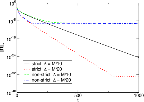
Figure 3: This figure shows the $L_{2}$ norm of $\Pi$ in a scalar field evolution outside the black hole for about 250 crossing times. The figure compares results for a naïve discretization (see text), and a strictly stable discretization at two resolutions, $\Delta=M/10$ and $\Delta=M/20$. The domain is $(x,y,z)\in[1.5,5.5]$, $\lambda=0.5$, and no dissipation is added to the solution.

To verify that we get the expected self-convergence factor in long term simulations when the fields do not decay to very small values after having left the domain, we now show results of a complementary set of tests on the domain $x\in[2.1M,6.1M]$, $(y,z)\in[-2M,2M]$. Here we concentrate in what corresponded to the worst case scenario considered, given by $\lambda=1$. We set the incoming modes on all outer faces to zero, except on the $x=6.1M$ face, where the time derivative of the incoming fields is set to

$$W_{+}=\left\{\begin{array}[]{ll}(y^{2}+z^{2}-M)^{6}(M/t-1)^{6}\sin(t)&\\ \qquad\qquad\qquad\mbox{if $t\geq 1$,}\mbox{$(y,z)\in[-M,M]$}&\\ 0\qquad\qquad\qquad\mbox{otherwise}&{}\end{array}\right.$$

This boundary condition is imposed through an orthogonal projection, as explained in Paper I. Initial data is given by

$$\Pi = 10^{7}\left[(x-3M)(x-4M)(y-M)(y+M)\right.$$ (59)

$$\qquad\times\left.(z-M)(z+M)\right]^{4}\;,$$

and both discretizations (strictly and non-strictly stable) are evolved. Figure 4 shows the self-convergence factor (as before, in the $L_{2}$ norm) of $\Phi$ and $\Pi$ versus time for the strictly stable discretization (similar factors are obtained for the non-strictly stable one) at the resolutions $\triangle=M/10$, $M/20$ and $M/40$. Convergence factors close to the expected value of two are observed, with no qualitative difference in the convergence factor as time progresses.

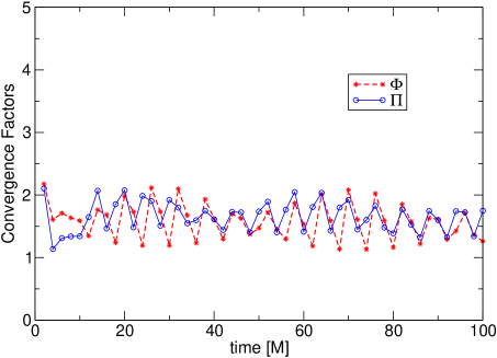
Figure 4: This figure shows the self-convergence factor as a function of time for the fields $\Pi$ (solid line) and $\Phi$ (dashed line) on a domain outside the black hole, using the strictly stable scheme (similar factors are obtained for the naive one), for about $25$ crossing times. These factors are calculated using resolutions of $M/10$, $M/20$, and $M/40$. The obtained factors are close to the expected value of two. The Courant factor is $\lambda=1$, and no dissipation is used.

V.1.2 Case 2: Domain with excision

In this section, the computational domain contains the black hole, which is excised with an inner cubic boundary centered on the black hole. The domain is defined on $[-4.5M,4.5M]^{3}$, and the excision cube has a total length of $0.6M$. Thus, the faces of the inner boundary are at $\pm 0.3M$.

We first verify that the excision algorithm does not display ALTI when employing the strictly stable scheme. As mentioned earlier, very little freedom is available in constructing difference operators that satisfy SBP. Indeed, for our second-order code with a diagonal scalar product, the stencils are uniquely specified. Figure 5 shows the $L_{2}$ norms of $\Pi$ and $\Phi$ for a long –up to $10^{4}M$– evolution (with no dissipation), designed to detect slowly growing modes. As shown in this figure, the algorithm specified by requiring SBP and the equations arranged so as to preserve the energy is long-term stable even with excision boundaries. For this run non-trivial initial data are given, as before, only to $\Pi$.

$$\Pi=\left\{\begin{array}[]{ll}\delta^{-8}r^{-1}\left[(r-r_{0})^{2}-\delta^{2}\right]^{3}(r0-r)&\mbox{if $|r-r_{0}|\leq|\delta|$}\\ 0&\mbox{otherwise \, .}\end{array}\right.$$ (62)

with $r_{0}=2.5M$ and $\delta=1.5M$. When studying the convergence of the code one again faces the fact that after a few crossing times the convergence value become meaningless. The behavior observed is analogous to the case where the black hole was outside the computational domain. Namely, close to second order convergence is seen during the first few crossing times, and unrealistically high values are obtained afterwards. In Fig. 6 we show a short-term convergence test (about two crossing times) with excision. Fig. 7 shows the corresponding $L_{2}$ norms for $\Phi$ and $\Pi$.

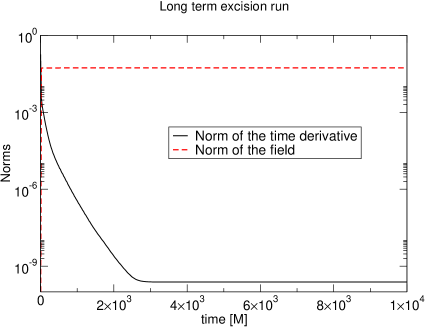
Figure 5: This figure demonstrates the long-term stability of the strictly stable discretization of the scalar wave equation when an excised black hole is on the grid. The $L_{2}$ norms of $\Pi$ (solid line) and $\Phi$ (dashed line) are shown for about 2500 crossing times. No slowly growing unstable modes are detected in these runs. This run was performed with $81^{3}$ grid points, $\lambda=0.25$, and no dissipation is used.

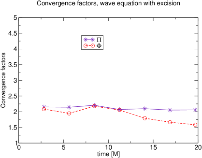
Figure 6: This figure shows a self-convergence test for $\Pi$ (solid line) and $\Phi$ (dashed line) using the same configuration as in Fig. 5. The self-convergence test is performed on uniform grids with $81^{3},161^{3}$, and $321^{3}$ grid-points. The convergence factor is close to the expected value of two. The measured convergence factor drops slightly from near two after one crossing time, when most of the field has left the domain and afterwards increases to unrealistic high values.

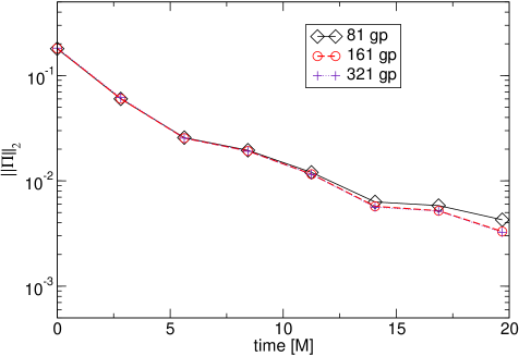
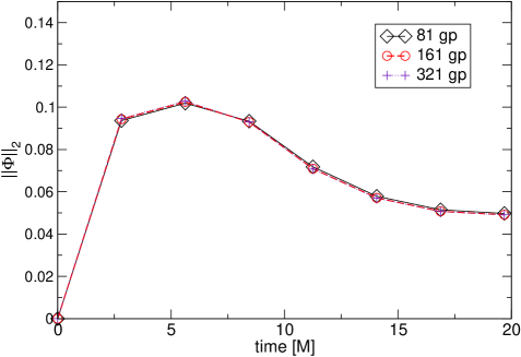
Figure 7: This figure shows $L_{2}$ norms for the runs shown in Fig.6. The relative difference in the norms for $\Phi$ at any two different resolutions, is at most about one percent. Similarly for $\Pi$, except at the last point shown, where this field has mostly left the grid.

As in the previous case, we also compare results obtained with the strictly stable and the naïve discretizations. Long term stability was found for both cases when the computational domain was outside the black hole. With excision, however, the solution obtained with the naïve discretization quickly becomes corrupted, as shown in Fig. 8. As shown in this figure, the amplitude decreases with resolution, indicating that the growth is spurious and that the naïve discretization suffers from ALTI. The strictly stable discretization, however, with a sharp semi-discrete energy estimate, remains well-behaved. The ALTI that contaminate the naïvely discretized solution are found to be of high-frequency type, which can be managed by adding explicit dissipation. Figure 9 shows results using the same initial configurations, except that now dissipation is added to the naïve discretization. Now all of the runs produce long term stable simulations.

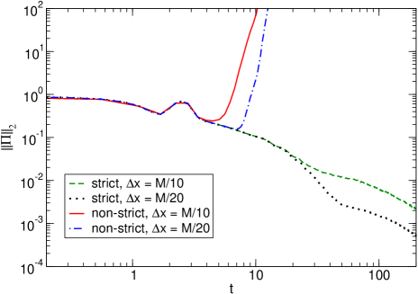
Figure 8: This figure shows the $L_{2}$ norm of $\Pi$ in a scalar field evolution on a domain containing an excised Schwarzschild black hole. The solid and dot-dashed lines show the $L_{2}$ norm of $\Pi$ obtained using the naïve discretization of the wave equation. Although the amplitude decrease with resolution, this solution quickly becomes long-term unstable, indicating an artificial instability. The strictly stable discretization (shown with dashed and dotted lines), however, remains long term stable and well-behaved. The results are calculated with the resolutions $\Delta=M/9$ and $\Delta=M/18$, $\lambda=0.5$, and no dissipation is added.

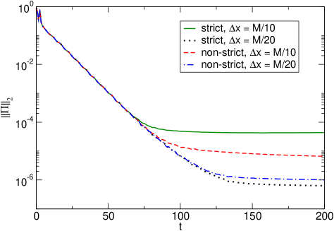
Figure 9: This figure shows the $L_{2}$ norm of $\Pi$ in a scalar field evolution on a domain containing an excised Schwarzschild black hole. The solid and dot-dashed lines show the solutions obtained using the naïve discretization with dissipation, the latter eliminating the artificial instability noted in Fig. 8. The strictly stable discretization (shown with dashed and dotted lines), without dissipation, is shown for comparison. The results are calculated with the resolutions $\Delta=M/9$ and $\Delta=M/18$, $\lambda=0.5$, and the dissipation parameter is $\sigma=0.02$.

V.2 Maxwell fields in a Schwarzschild background in PG coordinates

As with the scalar field tests above, we perform tests with the Maxwell equations on two kind of domains. Specifically, we choose

1. Computational domain outside the black hole: $y,z\in[-4M,4M]^{2}$ and $x\in[3M,11M]$;

2. Computational domain including part of the black hole: $(x,y,z)\in[-8.5M,8.5M]^{3}$. The singularity is excised by means of a cubical region defined by $(x,y,z)\in[-0.35M,0.35M]^{3}$.

The initial data describe a “pulse” of electromagnetic field given by

$$F_{i}=\left\{\begin{array}[]{ll}\alpha\delta^{-8}\left[(r-r_{0})^{2}-\delta^{2}\right]^{8}\epsilon_{ij3}(x^{j}-x_{o}^{j})&\mbox{if $|r-r_{0}|<\delta$}\\ 0&\mbox{otherwise \, ,}\end{array}\right.$$

where $F_{i}$ stands for $E_{i}$ and $B_{i}$, $\alpha$ is a strength parameter, $x_{o}^{i}$ is the location of the pulse’s center, and $\delta$ its width. We discretize in a strictly stable way, as explained in Section IV.1.2.

V.2.1 Case 1 (domain outside the black hole)

Let $\alpha=1$, $x_{o}^{i}=(7M,0,0)$ and $\delta=M$, and we set the dissipation to zero. Figure 10 shows $||E_{x}||_{2}$ vs. time for four different resolutions ($81^{3},161^{3},241^{3}$ and $321^{3}$ grid-points, corresponding to $\Delta=M/10,M/20,M/30$ and $M/40$, respectively), while the inset shows the decay in time for a long-term run with the coarsest resolution. Figure 11 shows the self-convergence factor of $E_{x}$ for a short time, computed with $81^{3}$, $161^{3}$ and $321^{3}$ grid-points, and $161^{3}$, $241^{3}$, and $321^{3}$ grid-points. As expected, the factor gets closer to two when resolution is increased.

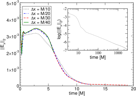
Figure 10: This figure shows the $L_{2}$ norm of $E_{x}$ vs.  time in an evolution of the Maxwell fields at four different resolutions for a strictly stable discretization. The computational domain is outside the black hole. The inset shows a long-term evolution, $3000M$, using the coarsest resolution. The runs were performed on uniform grids with resolutions $M/10$, $M/20$, $M/30$ and $M/40$, and the Courant factor is $\lambda=0.25$.

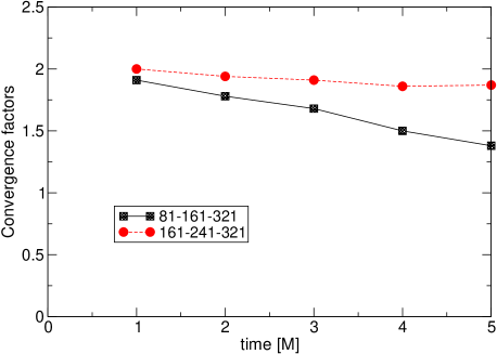
Figure 11: This figure shows self-convergence factors for $E_{x}$ for the runs of Fig. 10. The factors improve with resolution, in the sense that they closer to the expected value of two. The labels $81$-$161$-$321$ and $161$-$241$-$321$ indicate the number of grid points in each direction used to perform the self-convergence test.

V.2.2 Case 2: Domain with excised black hole

Now let $\alpha=1$, $x_{o}^{i}=(6.5M,0,0)$ and $\delta=M$. In contrast to the scalar field runs, solutions of the Maxwell equations without explicit dissipation diverge at long times, even with a strictly stable discretization. The reason for this appears to be that the energy inside the black hole is not positive definite and boundedness (either at the continuum or numerical level) is not guaranteed (it is not clear why this divergence does not appear in the scalar field case, when the singularity is excised, since the energy is also non-positive definite in that case.). High frequencies are seen in the solution, and we therefore add a small amount of dissipation, $\sigma=0.05$. Figures 12 and 13 show the norms and convergence data similar to the figures for the domain outside the black hole. As before, the simulations are long-term stable for long times. The self-convergence factors for the coarsest resolutions drop quickly from their initial value, indicating that the coarsest solutions are not in the convergent regime. In addition to effects caused by the fields leaving the computational domain, using a cubical excision boundary forces us to excise very close to the black hole, where the spacetime and field gradients are very large, effectively requiring higher resolution.

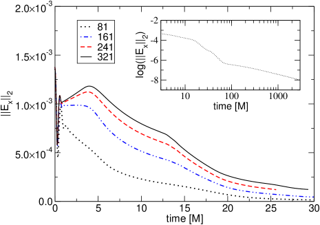
Figure 12: This figure shows the $L_{2}$ norm of $E_{x}$ vs.  time in an evolution of the Maxwell fields on a computational domain containing an excised black hole for a strictly stable discretization. The norms are shown for four different resolutions, and the inset shows a long-term evolution, $3000M$, at the coarsest resolution. The runs were performed on uniform grids with resolutions $M/10$, $M/20$, $M/30$ and $M/40$. The Courant factor is $\lambda=0.25$, and dissipation is added to the evolution equations, with $\sigma=0.05$.

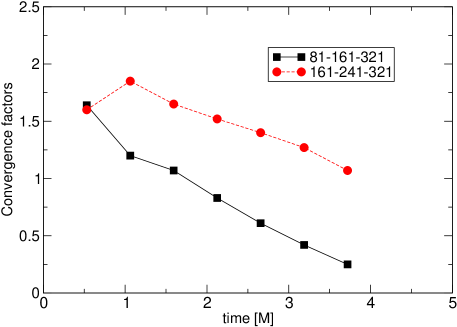
Figure 13: This figure shows convergence data for the runs of Fig. 12. The self-convergence factors are calculated from $E_{x}$. The excision boundary is very close to the black hole, and the large gradients encountered in the fields and spacetime near the excision boundary require very high resolution to resolve them adequately. The coarsest solutions are not resolved well enough to be in the convergence regime. However, it can be seen from the Figure that the convergence improves with resolution. The labels $81$-$161$-$321$ and $161$-$241$-$321$ indicate the number of grid points in each direction used to perform the self-convergence test.

V.3 Linearization around the gauge wave

The gauge wave is a useful test problem for examining some of the difficulties found in the simulation of the Einstein equations (see  convergence ; gaugeapples ; gaugejansen ; winicourgauge ), and to illustrate the usefulness of the techniques presented in Paper I. To this end, we present results obtained using a straight-forward discretization of the right hand side of Eqs. (46)–(50), and show results obtained for long term evolutions with and without dissipation. Moreover, we consider cases both where the constraints are initially satisfied, and where they are not. The latter illustrates that even when large constraint violations are introduced in the initial data, the solutions to the linearized equations remain well behaved. This, of course, may not necessarily be the case for the non-linear Einstein equations, as for these relatively large amplitudes the linearized system need not be a close approximation to the non-linear ones. Or even if the amplitudes were small, there could be purely non-linear effects in the solution which would naturally be missed in a linearized analysis sartom .

For these tests we adopt trivial initial data for all fields, except for $g_{xx}$, $d_{xxx}$ and $K_{xx}$, which have compact support in $x\in[0,1]$ and are given by

$$g_{xx} = \kappa\sin(x)\left[(x-0.5)^{2}-0.25\right]^{4},$$ (64)

$$d_{xxx} = \mu\partial_{x}g_{xx},$$ (65)

$$K_{xx} = -\frac{\xi}{2}\partial_{x}g_{xx}\,,$$ (66)

where $\kappa$, $\mu$, and $\xi$ are constants. We set $A=0.1$ in the background solution and the computational domain is taken to be $x\in[-0.5,1.5]$. Boundary conditions are applied via Olsson’s projection operators. Here, as we are interested in the long term behavior of the solution, we couple the incoming modes the outgoing ones such that

$$W_{+}=0.5W_{-}\;.$$

For cases where the constraints are initially satisfied, we choose $\mu=1=\xi$, $\kappa=0.01$; otherwise we set $\mu=0$, $\kappa=0.01$ and $\xi=1$. In all these simulations a Courant factor of $\lambda=0.25$ is used, to compare with similar simulations  convergence ; gaugeapples ; gaugejansen ; winicourgauge .

Figures 14-16 show results for constraint-satisfying initial data, without dissipation. Figure 14 shows the $L_{2}$ norm of the constraint, $C_{{\cal A}}$ and its convergence to zero with increasing resolution. Initially the norm $C_{{\cal A}}$ is almost constant. However, at later times a clear exponential mode is observed. While the solution is well-behaved for longer times with increasing resolution, this approach is impractical for long runs. Figure 15 shows the convergence (to zero) factors in the $L_{2}$ norm obtained for $C_{{\cal A}}$. For the highest resolutions, the factor is very close to its expected value.

An exponential behavior for $g_{xx}$ is also seen in Figure 16. Even though in principle this quantity could already grow at the continuum, the fact that at fixed time the norm of $g_{xx}$ decreases with increasing resolution suggests that, as discussed below, this is an artifact of an ALTI.

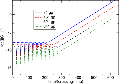
Figure 14: Logarithm of the $L_{2}$ norm of $C_{{\cal A}}$ vs. number of crossing times for four different resolutions. After an initial stage where the constraints are well behaved a clear exponential mode dominates the solution.

.

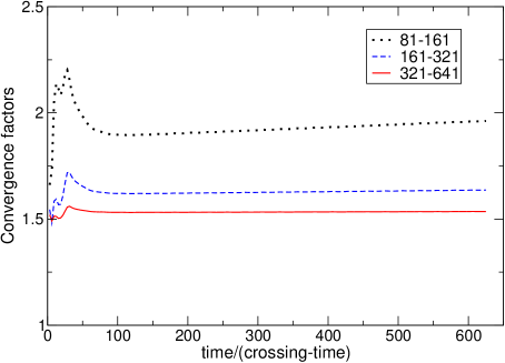
Figure 15: Convergence factors (to zero) for $C_{{\cal A}}$ as a function of number of crossing times, comparing runs with $81$ and $161$ points (dotted line), $161$ and $321$ points (dashed line) and $321$ and $641$ points (solid line). Notice that even when the solutions are growing exponentially (see Figs.14,16), the constraints converge to zero.

.

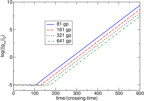
Figure 16: Logarithm of the $L_{2}$ norm of $g_{xx}$ vs. number of crossing times for four different resolutions with no dissipation. At early times, the norm remains fairly constant but at later ones an exponential growth dominates the solution.

.

The ALTI for $C_{{\cal A}}$ are, as in the previous examples, found to be of high frequency type and, therefore, the addition of dissipation eliminates these growing modes. Figures 17–20 illustrate the behavior of simulations with the same initial data and boundary conditions as those of Figures 14-16 , except that now some dissipation is added, $\sigma=0.01$. The norm of $C_{\cal A}$ is illustrated in Fig. 18, where now only a slow growth is observed at late times. Fig.  20 shows, as before, the convergence factors (to zero) for $C_{\cal A}$, in the $L_{2}$ norm. Finally, figure 17 shows the $L_{2}$ norm of $g_{xx}$ for different resolutions. Only a linear growth is observed in the solution is found; furthermore, this growth decreases with resolution.

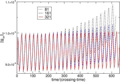
Figure 17: $L_{2}$ norm of $g_{xx}$ vs. number of crossing times for four different resolutions. Only a small growth is observed in the solution.

.

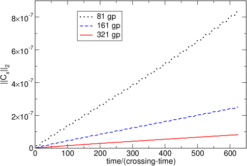
Figure 18: $L_{2}$ norm of $C_{{\cal A}}$ vs. number of crossing times for four different resolutions. Convergence to zero is observed and only slow (linear) growth is observed.

.

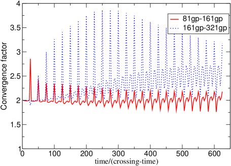
Figure 19: Convergence factors calculated with $C_{{\cal A}}$ vs. number of crossing times comparing runs with $81$ and $161$ points (dotted line), $161$ and $321$ points (solid line).

As a last example we consider initial data violating the constraints. Here, similarly good behavior is observed when dissipation is employed, in the sense that, as predicted by the continuum analysis of Section IV.2, the constraints oscillate in time. For instance, figure 20 shows the $L_{2}$ norm of the constraint $C_{x}$ vs. time. As expected, these converge to a roughly constant behavior as resolution is increased, and no growth is observed.

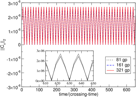
Figure 20: $L_{2}$ norm of $C_{x}$ vs. number of crossing times for three different resolutions, corresponding to the case where the initial data does not satisfy $C_{x}=0$. As expected from the continuum analysis, even in this case the norm does not grow in time.

VI Conclusions

The construction of stable numerical methods for IBVPs often involves a mixture of intuition and experimentation. The choice of numerical scheme and boundary conditions are often considered as necessarily separate ingredients. For certain problems, however, the energy method for discrete systems is an integrated, systematic method for creating numerically stable schemes and analyzing their behavior. While this method has not yet been widely used in general relativity, many current outstanding problems in the field vitally depend on understanding the subtle interplay of boundaries with the interior computational domain. In this paper we have applied the discrete energy method to test problems commonly found in numerical relativity and analyzed the numerical and long-term stability of the resulting schemes, with and without black hole excision. We have also investigated the numerical origin of fast growing modes which may artificially appear in numerical solutions, and used the energy method to discuss possible remedies.

In particular, we have presented explicit examples of the techniques described in paper I and discussed what leads to ALTI and a way to remove or alleviate them. A message from this work is that it is not sufficient to construct numerically stable implementations, but also special care must be taken to devise suitable numerical methods to rule out, or alleviate ALTI. (For a somewhat related approach, see the recent work winicourgauge ).

To illustrate how this is achieved we have adopted a series of examples, which although considerably simpler than Einstein equations, are relevant in the context of numerical relativity. In particular, in efforts to deal with black hole spacetimes and to understand the source of problems encountered with the gauge wave test. As shown throughout this work, even though there are examples in which low-frequency ALTI are present and for which no sharp estimate is known, a careful analysis and grouping of the variables and/or the addition of (controllable) artificial dissipation may in many cases be crucial in handling otherwise artificial long term instabilities.

It is expected that these techniques will be important in a number of fronts, in particular in the simulation of Einstein’s equations.

VII Acknowledgments

We wish to thank G. Calabrese, O. Sarbach, J. Pullin, E. Tadmor, P. Olsson, and H.-O. Kreiss for helpful discussions, and E. Schnetter for helpful comments on the manuscript. This work was supported in part by NSF grants PHY0244699, PHY0312049; NASA-NAG5-1430; the Horace Hearne Jr. Lab for Theoretical Physics, CONICET, and SECYT-UNC. Computations were done at LSU’s Center for Computation and Technology and parallelized with the CACTUS toolkit cactus . L.L. is an Alfred P. Sloan Fellow.

Appendix A Cubic excision for Kerr black holes

Black hole excision removes the singularity by placing an inner boundary on the computational domain. While the boundary removes the singularity, the question now becomes finding physically and mathematically consistent inner boundary conditions. Clearly, a general solution to this problem for an arbitrary boundary is unknown. The time-development of this boundary presents a further complication. Namely, if the boundary becomes time-like, it will encounter the singularity in a finite amount of time. These two issues can be resolved simultaneously by adopting an inner boundary with a space-like world tube. This ensures it will not hit the singularity and that no boundary conditions are necessary if all the characteristics speeds are within the light cone, as the past domain of dependence of boundary points is wholly contained on the previous time slice. Some freedom remains in choosing the particular region to be excised, and clearly the largest possible excision boundary is preferable to avoid the strongest gradients of the spacetime.

To illustrate some of these issues we now examine cubical excision for both the Schwarzschild and Kerr black holes, looking for the largest possible space-like excision cube. As we discuss below, the shape of the boundary plays a crucial role in satisfying the spacelike condition. We examine one face of the cube, a $x=\mbox{const}$ face. The condition that this surface is space-like implies that $g^{xx}<0$, as $\nabla_{x}$ is the normal to the surface. Since the coordinates are fixed a-priori, we can only vary the position of the boundary to meet this condition. We find that this condition is quite difficult to satisfy, and possible for only very slowly spinning black holes.

To see this in detail, consider the Kerr metric in Kerr–Schild form kerrschild . The quantity $g^{xx}$ is

$$g^{xx}=1-2\frac{Mr^{3}}{r^{4}+a^{2}z^{2}}\left(\frac{rx+ay}{r^{2}+a^{2}}\right)^{2},$$ (67)

where $r$ is related to the Cartesian coordinates by

$$\frac{x^{2}+y^{2}}{r^{2}+a^{2}}+\frac{z^{2}}{r^{2}}=1\,.$$ (68)

The space-like character requirement on the surface implies that

$$2\frac{Mr^{3}}{r^{4}+a^{2}z^{2}}\left(\frac{rx+ay}{r^{2}+a^{2}}\right)^{2}>1\,.$$ (69)

For the Schwarzschild black hole, $a=0$, $r^{2}=x^{2}+y^{2}+z^{2}$, and the above condition becomes

$$2\frac{Mx^{2}}{r^{3}}>1.$$ (70)

The corner of the cube is the limiting point ($y=z=x$) for the largest cube, giving the bound $x<2M/(3\sqrt{3})$, or $x\lesssim 0.385M$.

For the spinning black hole, the analysis is slightly more involved. The limiting point for the largest cube is given by $y=-x$, $z=\pm x$, giving the condition

$$\frac{2M\sqrt{2}x^{3}(\sqrt{3}x-{2}^{-1/2}a)^{2}}{(3x^{2}+a^{2})^{2}}>\frac{4x^{2}+a^{2}2^{-1/2}}{2}.$$ (71)

Examining this condition shows that cubical excision can not be used when $a\gtrsim 0.082$, as shown in Fig. 21. Furthermore, the singularity is not at a point, but is ring-like, implying that the cube may not be arbitrarily small. Finding the minimum sized cube is more involved, as the faces of the cube need to be examined in addition to the corners gioeldave .

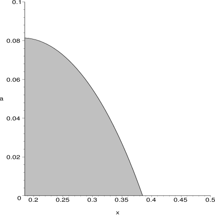
Figure 21: The shaded region indicates, for a given value of $a$, the size of the maximum allowed cubical region that satisfies Eq. 71. Clearly, the allowed values of $a$ are restricted below $\lesssim 0.082$.

.

This limitation of cubical excision for the Schwarzschild spacetime was noted before markITP , by requiring that the excision boundary has no in-coming modes in a particular formulation of Einstein equations. A similar analyzis to that of markITP for the Kerr spacetime and cubical excision regions has also recently presented in gioeldave . Here we would like to point out the following. First, when the eigenmodes are complete and the speeds are physical (they lie within the null cone) those results and the one presented here are equivalent, as it is rooted in the physical nature of the excision boundary. Second, when dealing with a formulation admitting eigenspeeds outside the light cone, or a non-complete set of eigenmodes, the current straightforward analysis provides necessary conditions that have to be met. These necessary conditions are useful when dealing with any formulation, in particular one whose eigenspeeds might not be known. Finally, we emphasize that these results are coordinate dependent; nevertheless, for the families often used in numerical relativity tests, the same result applies. In particular for the family of slicings reported by Martel and Poisson martelpoisson (which contains both the Kerr–Schild and Painlevé–Gullstrand slicings of Schwarzschild).

References

- (1) R. Arnowitt, S. Deser, and C. Misner, in Gravitation: An Introduction to Current Research, edited by L. Witten (Wiley, New York, 1962).
- (2) L. Lehner, Class. Quant. Grav. 18, R25 (2001).
- (3) T. W. Baumgarte and S. L. Shapiro, Phys. Rept. 376, 41 (2003).
- (4) C. Gundlach, Living Reviews 1999-4, published electronically on http://www.livingreviews.org.
- (5) B. Gustaffsson, H.-O. Kreiss, and J. Oliger, Time Dependent Problems and Difference Methods (Wiley, New York, 1995).
- (6) G. Calabrese, J. Pullin, O. Sarbach and M. Tiglio, Phys. Rev. D 66, 064011 (2002).
- (7) G. Calabrese, L. Lehner, O. Reula, O. Sarbach, and M. Tiglio, gr-qc/0308007.
- (8) P.D. Lax, Comm. Pure Appl. Math. VII, 159 (1954).
- (9) H. Friedrich and A. Rendall, in Einstein’s Field Equations and their Physical Implications, Lecture Notes in Physics”, edited by B. G. Schmidt (Springer-Verlag, Berlin, 2000), pp. 127-223; O. Reula, Living Rev. Relativ. 1, 3 (1998).
- (10) H.-O. Kreiss and G. Scherer, SIAM Journal on Num. Anal. 29, 640, (1992).
- (11) P. Olsson Mathematics of Computation 64, 1035 (1995); Mathematics of Computation 64, S23 (1995); Mathematics of Computation 64, 1473 (1995).
- (12) H.-O. Kreiss and L. Wu, Appl. Numr. Math. 12, 213 (1993)
- (13) D. Levy and E. Tadmor, SIAM Journal on Num. Anal. 40, 40, (1998).
- (14) W. Unruh, cited in tho .
- (15) J. Thornburg, Class. Quantum Grav., 4, 1119 (1987).
- (16) B. Strand, Journal of Computational Physics 110, 47 (1994).
- (17) H. Friedrich, Comm. Math. Phys. 107, 587 (1987).
- (18) D. Christodoulou and S. Klainerman. The Global Nonlinear Stability of Minkowski Space, Princeton Univ. Press., Princeton (1993).
- (19) S. Klainerman and I. Rodnianski. “The causal structure of microlocalized Einstein metrics”, math.AP/0109174 (2001).
- (20) M. Tiglio, L. Lehner and D. Neilsen, “3D simulations of Einstein’s equations: symmetric hyperbolicity, live gauges and dynamic control of the constraints,” arXiv:gr-qc/0312001.
- (21) G. Calabrese, L. Lehner, D. Neilsen, J. Pullin, O. Reula, O. Sarbach and M. Tiglio, Class. Quant. Grav. 20, L245 (2003).
- (22) G. Calabrese and D. Neilsen, Phys. Rev. D 69, 044020 (2004).
- (23) M. Alcubierre and B. F. Schutz, J. Comput. Phys. 112, 44 (1994)
- (24) M. A. Scheel, T. W. Baumgarte, G. B. Cook, S. L. Shapiro and S. A. Teukolsky, Phys. Rev. D 56, 6320 (1997)
- (25) M. Alcubierre and B. Brugmann, Phys. Rev. D 63, 104006 (2001)
- (26) H. J. Yo, T. W. Baumgarte and S. L. Shapiro, Phys. Rev. D 64, 124011 (2001)
- (27) D. Shoemaker, K. Smith, U. Sperhake, P. Laguna, E. Schnetter and D. Fiske, Class. Quant. Grav. 20, 3729 (2003)
- (28) M. Anderson and R. A. Matzner, arXiv:gr-qc/0307055.
- (29) L. E. Kidder, M. A. Scheel, S. A. Teukolsky, E. D. Carlson and G. B. Cook, Phys. Rev. D 62, 084032 (2000) [arXiv:gr-qc/0005056].
- (30) M. Scheel, Talk at “Miniprogram on Colliding Black holes: Mathematical Issues in Numerical Relativity”, Institute for Theoretical Physics, University of California at Santa Barbara, January 10-28,2000.
- (31) O. Sarbach and M. Tiglio, Phys. Rev. D 66, 064023 (2002). [arXiv:gr-qc/0205086].
- (32) M. Alcubierre et al., arXiv:gr-qc/0305023.
- (33) E. Schnetter, S. H. Hawley and I. Hawke, Class. Quant. Grav. 21, 1465 (2004) [arXiv:gr-qc/0310042].
- (34) N. Jansen, B. Bruegmann and W. Tichy, arXiv:gr-qc/0310100.
- (35) O. Sarbach and M. Tom, in preparation.
- (36) M. Babiuc, B. Szilagyi and J. Winicour, arXiv:gr-qc/0404092.
- (37) http://www.cactuscode.org
- (38) R.P. Kerr and A. Schild, in Applications of Nonlinear Partial Differential Equations in Mathematical Physics, Proc. of Symposia b Applied Math, XVII, (1965).
- (39) K. Martel and E. Poisson, Phys. Rev. D 66, 084001 (2002).