Construction and enlargement of traversable wormholes from Schwarzschild black holes

Abstract

Analytic solutions are presented which describe the construction of a traversable wormhole from a Schwarzschild black hole, and the enlargement of such a wormhole, in Einstein gravity. The matter model is pure radiation which may have negative energy density (phantom or ghost radiation) and the idealization of impulsive radiation (infinitesimally thin null shells) is employed.

I Introduction

While black holes are now almost universally accepted as astrophysical realities, traversable wormholes are still a theoretical idea MT ; V . Yet they are both predictions of General Relativity in a sense, though black holes require positive-energy matter (or vacuum) whereas wormholes require negative-energy matter. While normal positive-energy matter was long thought to dominate the universe, it is now known that this is not so. The recently discovered acceleration of the universe Spe ; Kra indicates that its evolution is dominated by unknown dark energy which violates at least the strong energy condition ($w\geq-1/3$ to cosmologists, where $w$ is the ratio of pressure to density in relativistic units, for a homogeneous isotropic cosmos), and perhaps also the weak energy condition ($w\geq-1$), where it is known as phantom energy Cal . Such phantom energy is precisely what is needed to support traversable wormholes HV1 ; HV2 ; wh ; IH .

While black holes and traversable wormholes have been regarded by most experts as quite different, one of the authors has argued that they form a continuum and are theoretically interconvertible wh . Specifically, both are locally characterized by trapping horizons wh ; IH ; 1st ; bhd , which are the Killing horizons of a stationary black hole and the throat of a stationary wormhole. The difference is the causal nature, being spatial or null for a black hole and temporal for a wormhole. This in turn depends on whether the energy density is positive, zero or negative. If the energy density can be controlled, it should be possible to dynamically create a traversable wormhole from a black hole and vice versa. This was first concretely demonstrated in a two-dimensional model HKL , but it is more difficult in full General Relativity. Numerical simulations have been used to study a wormhole supported by a ghost (or phantom) scalar field, showing that it does indeed collapse to a black hole if perturbed by positive-energy matter SH . (We use phantom to mean that the energy density has the opposite sign to normal, which is equivalent in our cases to the convention for ghost fields in quantum field theory, that the kinetic energy has the opposite sign). As for analytic results, one simple case is a static wormhole supported by pure ghost (or phantom) radiation pr ; it is easy to see that if the radiation is switched off, it immediately collapses to a Schwarzschild black hole. The converse, creating a traversable wormhole from a Schwarzschild black hole, is more complex and is the first main result of this article.

As above, we use pure phantom radiation as the exotic matter model. We also employ the idealization of impulsive radiation, where the radiation forms an infinitesimally thin null shell, thereby delivering finite energy-momentum in an instant KHK . Space-time regions can be matched across such shells using the Barrabès-Israel formalism B-I . This allows an ingenious analytic construction of the desired type of solution, by matching Schwarzschild, static-wormhole and Vaidya regions, the latter consisting of pure radiation propagating in a fixed direction Vaidya . Our other main result is the similar construction of analytic solutions describing the enlargement or reduction of such a wormhole. Then if Wheeler’s space-time foam picture Whe is correct and Planck-sized virtual black holes are continually forming, we have exact solutions in standard Einstein gravity describing how they may be converted into traversable wormholes and enlarged to usable size. Our results have been summarized in a shorter article HK .

Our paper is organized as follows. In Sec. II, we briefly review the static wormhole solutions with pure phantom radiation, and the Schwarzschild and Vaidya solutions. In Sec. III we show how to join these basic solutions at null boundaries. In Secs. IV and V we present analytic solutions which describe respectively the construction and enlargement of a wormhole. In Sec. VI we consider the jump in energy due to impulsive radiation, as a check that the matchings are physically reasonable, and as a simple way to understand the changes in area of the wormhole throat or black-hole horizon. The final section is devoted to summary.

II Basic solutions

In this section we review the traversable wormhole solution pr , the Schwarzschild solution and the Vaidya solutions in the various coordinates needed. We will consider spherically symmetric space-times only. It is convenient to use the area radius $r=\sqrt{A/4\pi}$, where $A$ is the area of the spheres of symmetry. Although we often use $r$ as a coordinate, it is a geometrical invariant of the metric and is assumed throughout to be continuous. A useful quantity is the local gravitational mass-energy MS ; sph

$$E=\frac{r}{2}(1-g^{\mu\nu}r_{,\mu}r_{,\nu}).$$ (1)

Note that $E=r/2$ on a trapping horizon, where $g^{\mu\nu}r_{,\mu}r_{,\nu}=0$, including both black-hole horizons bhd and wormhole mouths wh . The energy-momentum tensor of pure radiation (or null dust) is $T_{ab}=\rho u_{a}u_{b}$, where $u_{a}$ is null and $\rho$ is the energy density. Normally $\rho\geq 0$, but $\rho<0$ defines pure phantom radiation.

II.1 Static wormhole solution with pure phantom radiation

The static wormhole solutions pr supported by opposing streams of pure phantom radiation can be written as

$$ds^{2}=-\frac{2\lambda}{1+2l\phi e^{l^{2}}}dt^{2}+\frac{1+2l\phi e^{l^{2}}}{2\phi^{2}e^{2l^{2}}}dr^{2}+r^{2}d\Omega^{2}$$ (2)

where $t$ is the static time coordinate and $d\Omega^{2}$ refers to the unit sphere. Here $l$ is a function of $r$,

$$r=a(e^{-l^{2}}+2l\phi),$$ (3)

and $\phi$ is an error function,

$$\phi(l)\equiv\int_{0}^{l}e^{-\ell^{2}}d\ell+b,$$ (4)

where $a>0$, $b$ and $\lambda>0$ are constants.

The local energy evaluates as $E=\epsilon$ where

$$\epsilon=\frac{a}{2}(e^{-{l}^{2}}+2l\phi-2e^{{l}^{2}}\phi^{2}).$$ (5)

Using the mass-energy $\epsilon$, the metric (2) is rewritten as

$$ds^{2}=-\frac{\lambda}{e^{2l^{2}}\phi^{2}}\left(1-\frac{2\epsilon}{r}\right)dt^{2}+\left(1-\frac{2\epsilon}{r}\right)^{-1}dr^{2}+r^{2}d\Omega^{2}.$$ (6)

In the case $b=0$, the solutions (2) or (6) describe symmetric wormholes. The spacetime is not asymptotically flat, but otherwise constitutes a Morris-Thorne wormhole. The $b\neq 0$ cases include asymmetric wormholes which are analogous to the asymmetric Ellis wormhole for a phantom Klein-Gordon field Ellis . For the space-time solution to be a wormhole, the inequality

$$|b|<b_{cr}=\frac{\sqrt{\pi}}{2}$$ (7)

is needed. For any other value of $b$, a singularity is present. Hereafter, we consider $b=0$, describing a symmetric wormhole with minimal surfaces at the wormhole throat $l=0$, with area radius $r=a$.

The solutions (6) may be written in dual-null form

$$ds^{2}=-\frac{2\lambda}{1+2le^{l^{2}}\phi}dx^{+}dx^{-}+r^{2}d\Omega^{2}$$ (8)

where the null coordinates $x^{\pm}$ are defined by

$$dx^{\pm}=dt\pm\frac{a}{\sqrt{\lambda}}\left(e^{-l^{2}}+2l\phi\right)dl.$$ (9)

Then the radial null geodesics are given by constant $x^{\pm}$. We need the metric (6) in both ingoing and outgoing radiation coordinates:

$$ds^{2}=-\frac{\sqrt{\lambda}}{e^{l^{2}}\phi}dx^{\pm}\left[\frac{2\sqrt{\lambda}e^{l^{2}}\phi}{(1+2le^{l^{2}}\phi)}dx^{\pm}\mp 2dr\right]+r^{2}d\Omega^{2}.$$ (10)

In these coordinates the radial null geodesics are the lines of constant $x^{\pm}$ (choosing one) and the curves given by

$$\frac{dr}{dx^{\pm}}=\pm\frac{\sqrt{\lambda}e^{l^{2}}\phi}{(1+2le^{l^{2}}\phi)}.$$ (11)

The Penrose diagram is shown by Fig.1 (ii). The energy-momentum tensor supporting the wormhole is found to be

$$T_{ab}=-\frac{\lambda}{8\pi r^{2}}(\delta^{+}_{a}\delta^{+}_{b}+\delta^{-}_{a}\delta^{-}_{b}).$$ (12)

This is the energy tensor of two opposing streams of pure phantom radiation, with $\lambda=-4\pi r^{2}T_{tt}$ being the resulting negative linear energy density. On the other hand, the solutions with pure radiation of the usual positive energy density were founded by Gergely Gergely .

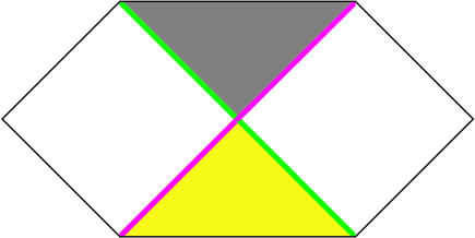
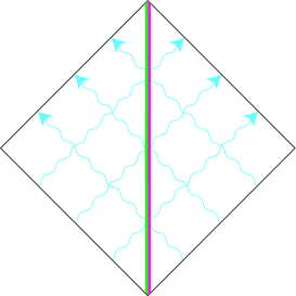
Figure 1: (Color online). Penrose diagrams of (i) a Schwarzschild black hole and (ii) a Hayward traversable wormhole pr . The bold magenta and green lines represent the trapping horizons, $\partial_{+}r=0$ and $\partial_{-}r=0$, respectively, which constitute the event horizons of the black hole and the throat of the wormhole. Yellow (light) and gray (dark) quadrants represent past trapped and future trapped regions, respectively. Wavy cyan lines represent the constant-profile radiation supporting the wormhole structure.

II.2 Schwarzschild solution

The Schwarzschild metric is given by

$$ds^{2}=-\left(1-\frac{2M}{r}\right)dt^{2}+\left(1-\frac{2M}{r}\right)^{-1}dr^{2}+r^{2}d\Omega^{2},$$ (13)

where the constant $M$ is the Schwarzschild mass, which coincides with the local energy, $E=M$. Rewriting in Eddington-Finkelstein coordinates

$$V=t-\zeta\left(r+2M\ln(1-r/2M)\right)$$ (14)

one finds

$$ds^{2}=-dV\left[\left(1-\frac{2M}{r}\right)dV+2\zeta dr\right]+r^{2}d\Omega^{2},$$ (15)

where $\zeta$ is a sign factor: $\zeta$ is $1$ for outgoing radiation or $-1$ for ingoing radiation, where this means that the area respectively increases or decreases along the future-null generators. The Penrose diagram is shown by Fig.1 (i).

II.3 Vaidya solutions

The metric of the Vaidya solutions is given by

$$ds^{2}=-dV\left[\left(1-\frac{2m(V)}{r}\right)dV+2\zeta dr\right]+r^{2}d\Omega^{2},$$ (16)

where $\zeta$ is a sign factor, where $\zeta=1$ for outgoing radiation, and $\zeta=-1$ for ingoing radiation. The mass function $m$ coincides with the local energy, $E=m$. The corresponding energy-momentum tensor is given by

$$T_{\mu\nu}=-\frac{\zeta}{4\pi r^{2}}\frac{dm}{dV}\delta^{V}_{\mu}\delta^{V}_{\nu}.$$ (17)

III Matching Vaidya regions to static-wormhole and Schwarzschild regions

In this section, we derive the matching formulas between Schwarzschild, Vaidya and static-wormhole regions along null hypersurfaces, following the Barrabès-Israel formalism B-I . This is a preliminary to constructing the wormhole-construction and wormhole-enlargement models.

III.1 Matching Vaidya and Schwarzschild regions

Firstly we consider the matching between Schwarzschild and Vaidya regions. We start by writing Schwarzschild and Vaidya solutions in the form

$$ds^{2}=-e^{\psi}dV(fe^{\psi}dV+2\zeta dr)+r^{2}d\Omega^{2},$$ (18)

where the metric functions are

$$f_{S}=1-\frac{2M}{r},\qquad\psi_{S}=0$$ (19)

for Schwarzschild, and

$$f_{V}=1-\frac{2m(V)}{r},\qquad\psi_{V}=0$$ (20)

for Vaidya.

Now we consider the boundary surface $V=V_{0}$ (constant). The normal to the hypersurface $\Phi=V-V_{0}=0$ is $n_{\mu}=\zeta\alpha^{-1}\partial_{\mu}\Phi=\zeta\alpha^{-1}\delta^{V}_{\mu}$, where $\alpha$ is a positive function. (Barrabès & Israel took $\alpha<0$). For a null hypersurface, the normal is also tangent, so to obtain extrinsic curvature one needs a different vector. From $n_{\mu}$ Barrabès and Israel introduced a so-called transverse null vector $N_{\mu}$ by requiring $N_{\mu}N^{\mu}=0$, and $N_{\mu}n^{\mu}=-1$. Without loss of generality, we assume that $N_{\mu}$ takes the form $N_{\mu}=N_{V}\delta^{V}_{\mu}+N_{r}\delta^{r}_{\mu}$, and choose the arbitrary function $\alpha$ as $\alpha=e^{-\psi}$. Then $N_{\mu}$ is given by

$$N_{\mu}=\zeta\frac{fe^{\psi}}{2}\delta^{V}_{\mu}+\delta^{r}_{\mu}.$$ (21)

Choosing the coordinates $r,\theta$, and $\varphi$ as the three intrinsic coordinates $\xi^{a}\equiv(r,\theta,\varphi),\;(a=1,2,3)$ on the hypersurface $V=V_{0}$, we find

$$e^{\mu}_{(1)}=\delta^{\mu}_{r},\;\;\;e^{\mu}_{(2)}=\delta^{\mu}_{\theta},\;\;\;e^{\mu}_{(3)}=\delta^{\mu}_{\varphi},$$ (22)

where $e^{\mu}_{(a)}\equiv\partial x^{\mu}/\partial\xi^{a}$. Then, it can be shown that the transverse extrinsic curvature, defined by B-I

$${\cal{R}}_{ab}=-N_{\mu}e^{\nu}_{(b)}\left(\nabla_{\nu}e^{\mu}_{(a)}\right),$$ (23)

takes the form

$${\cal{R}}_{ab}=diag.\left\{\zeta\frac{\partial\psi}{\partial r},\;-\zeta\frac{rf}{2},\;-\zeta\frac{rf}{2}\sin^{2}\theta\right\}.$$ (24)

The jump in transverse extrinsic curvature is denoted by

$$\gamma_{ab}=2[{\cal{R}}_{ab}].$$ (25)

Once $\gamma_{ab}$ is given, using the formula B-I

$$\tau^{ab}=-S^{ab}=\frac{1}{16\pi}(g^{ac}_{*}l^{b}l^{d}+g^{bd}_{*}l^{a}l^{c}-g^{ab}_{*}l^{c}l^{d}-g^{cd}_{*}l^{a}l^{b})\gamma_{cd},$$ (26)

we can calculate the surface energy-momentum tensor $\tau^{ab}$ on the null hypersurface $V=V_{0}$. In components,

$$\tau^{ab}=\sigma l^{a}l^{b}+Pg^{ab}_{*},$$ (27)

where

$$g^{ab}_{*} = r^{-2}\left(\delta^{a}_{\theta}\delta^{b}_{\theta}+\sin^{-2}\theta\delta^{a}_{\varphi}\delta^{b}_{\varphi}\right),$$ (28)

$$l^{a}=\delta^{a}_{r},\;\;\;\;\;\;l^{b}l_{b}=0.$$

Here $\sigma$ represents the surface energy density of the null shell and $P$ the pressure in the $\theta$ and $\varphi$ directions. Then

$$\sigma = \zeta\frac{[f]}{8\pi r}=\eta_{1}\zeta\frac{M-m(V_{0})}{4\pi r^{2}},$$

$$P = -\frac{\zeta}{8\pi}\left[\frac{\partial\psi}{\partial r}\right]=0.$$ (29)

We take the sign factor $\eta_{1}$ to be $1$ if the radiation is to the future of the Schwarzschild region, and $-1$ if the radiation is to the past of the Schwarzschild region (Fig.2). The energy-momentum tensor of the impulsive radiation is given generally by B-I

$$T^{\mu\nu}=\alpha\tau^{\mu\nu}\delta(\Phi),$$ (30)

where $\delta$ denotes the Dirac delta distribution. In our case it reduces to

$$T^{rr}=\tau^{rr}\delta(V-V_{0})=\eta_{1}\zeta\frac{[M-m(V_{0})]}{4\pi r^{2}}\delta(V-V_{0}).$$ (31)

Figure 2: Matching domains: $\eta_{1}=1$ (left) and $\eta_{1}=-1$ (right).

III.2 Matching Vaidya and static-wormhole regions

Secondly we consider matching Vaidya and static-wormhole regions. We rewrite the static wormhole solution (10) as

$$ds^{2}=-e^{\psi}du(f_{W}e^{\psi_{W}}du-2\zeta dr)+r^{2}d\Omega^{2},$$ (32)

where $u$ is $x^{\pm}$ for $\zeta=\pm 1$. The metric functions $f_{W}$ and $\psi_{W}$ are defined as

$$f_{W}=1-\frac{2\epsilon}{r},\qquad e^{\psi_{W}}=\frac{\sqrt{\lambda}}{e^{l^{2}}\phi}.$$ (33)

Now we consider the boundary surface $u=u_{0}$ (constant). Then, from the previous subsection, the transverse extrinsic curvature takes the form

$${\cal{R}}^{+}_{ab}=diag.\left\{-\zeta\frac{\partial\psi_{W}}{\partial r},\;\zeta\frac{rf_{W}}{2},\;\zeta\frac{rf_{W}}{2}\sin^{2}\theta\right\}.$$ (34)

On the other hand, we write the Vaidya solution Vaidya in the same form as (20)

$$ds^{2}=-e^{\psi_{V}}dV(f_{V}e^{\psi_{V}}dV+2\zeta dr)+r^{2}d\Omega^{2},$$ (35)

where the metric $f_{V}$ and $\psi_{V}$ is defined by (20). The hypersurface $u=u_{0}$ in the $(V,r)$ coordinates can be written as $\Phi^{-}=V-V_{0}(r)=0$, where $V_{0}(r)$ is a solution of the equation

$$\frac{dV_{0}}{dr}=-\zeta\frac{2}{f_{V}}e^{-\psi_{V}},\;\;\;(u=u_{0}).$$ (36)

Then the normal to the surface is given by

$$n^{-}_{\mu}=\zeta\beta^{-1}\partial_{\mu}\Phi^{-}=\zeta\beta^{-1}\left(\delta^{V}_{\mu}+\frac{2}{f_{V}}e^{-\psi_{V}}\delta^{r}_{\mu}\right),$$ (37)

where $\beta$ is a negative and otherwise arbitrary function. From $n^{-}_{\mu}$ we can also introduce the transverse null vector $N^{-}_{\mu}$, by requiring $N^{-}_{\mu}N^{-\mu}=0$, and $N^{-}_{\mu}n^{-\mu}=-1$. It can be shown that it takes the form

$$N^{-}_{\mu}=\zeta\frac{\beta f_{V}}{2}e^{2\psi_{V}}\delta^{V}_{\mu}.$$ (38)

The basis vectors are

$$e^{-\mu}_{(1)}=-\zeta\frac{2}{f_{V}}e^{-\psi_{V}}\delta^{\mu}_{V}+\delta^{\mu}_{r},\;\;\;e^{-\mu}_{(2)}=\delta^{\mu}_{\theta},\;\;\;e^{-\mu}_{(3)}=\delta^{\mu}_{\varphi},$$ (39)

where $e^{-\mu}_{(a)}\equiv\partial x^{\mu}_{-}/\partial\xi^{a}$. To be sure that the two transverse vectors $N^{\pm}_{\mu}$ defined in the two faces of the hypersurface $u=u_{0}$ represent the same vector, we need to impose the condition

$$N^{+}_{\lambda}e^{+\lambda}_{(a)}|_{u=u_{0}}=N^{-}_{\lambda}e^{-\lambda}_{(a)}|_{u=u_{0}},$$ (40)

which requires that the function $\beta$ has to be $\beta=-\exp\{-\psi_{-}\}$. Once $N^{-}_{\lambda}$ and $e^{-\lambda}_{(a)}$ are given, using Eq.(23) we can calculate the corresponding transverse extrinsic curvature, which in the present case takes the form

$${\cal{R}}^{-}_{ab}=diag.\left\{-\zeta\frac{2e^{-\psi_{V}}}{f_{V}^{2}}\frac{\partial f_{V}}{\partial V},\;\zeta\frac{rf_{V}}{2},\;\zeta\frac{rf_{V}}{2}\sin^{2}\theta\right\}.$$ (41)

Then, from Eqs.(41) and (34), we find the surface energy-momentum tensor (26) on the null hypersurface $u=u_{0}$, composed of the surface energy density $\sigma$ of the null shell and the pressures $P$ in the $\theta$- and $\varphi$-directions (27), as

$$\sigma = \eta_{2}\zeta\frac{f_{W}-f_{V}}{8\pi r}=-\eta_{2}\zeta\frac{\epsilon(r)-m(r)}{4\pi r^{2}},$$

$$P = \frac{\eta_{2}\zeta}{8\pi}\left(\frac{2e^{-\psi_{V}}}{f_{V}^{2}}\frac{\partial f_{V}}{\partial V}-\frac{\partial\psi_{W}}{\partial r}\right)=\frac{\eta_{2}\zeta}{4\pi}\left[\frac{dm(r)}{dr}-\frac{m(r)r}{2a^{2}\phi^{2}}+\frac{r^{2}}{4a^{2}\phi^{2}}\right],$$ (42)

where $m(r)$ is the mass function of the Vaidya region on the boundary $u=u_{0}$,

$$m(r)\equiv m(V)|_{u=u_{0}}.$$ (43)

Here we take the sign factor $\eta_{2}$ to be $1$ if the radiation is to the past of the wormhole region, and to be $-1$ if the radiation is to the future of the wormhole region (Fig.3). In calculating the above equation, we have not used the particular expressions for the functions $\psi$ and $f$. Thus, it is valid generally in the case that the boundary surface is $u=$constant.

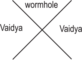
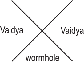
Figure 3: Matching domains: $\eta_{2}=1$ (left) and $\eta_{2}=-1$ (right).

Henceforth we consider only the dust shell case $P=0$, then we require

$$\frac{dm}{dr}-\frac{mr}{2a^{2}\phi^{2}}+\frac{r^{2}}{4a^{2}\phi^{2}}=0.$$ (44)

Integrating Eq.(44), we obtain

$$m=\frac{a}{2}(e^{-l^{2}}+2l\phi(l)-2\phi(l)^{2}e^{l^{2}})+C\phi(l)e^{l^{2}},$$ (45)

where $C$ is an integration constant and related to $\sigma$ by

$$\sigma=\eta_{2}\zeta C\frac{\phi e^{l^{2}}}{4\pi r^{2}}.$$ (46)

Then if there is no light-like shell, $\sigma=0$ and the mass function is continuous across the boundary surface, $\epsilon=m$. Extending the relation (36) to the Vaidya region, introducing $z(V)$ with $z=l$ on the boundary surface, we obtain the mass function of the Vaidya solutions beyond the boundary surface

$$m(z)=\frac{a}{2}(e^{-z^{2}}+2z\phi(z)-2\phi(z)^{2}e^{z^{2}})+C\phi(z)e^{z^{2}}$$ (47)

where the relation between $z$ and $V$ is

$$V(z)=-\zeta\int^{z}\frac{2a^{2}e^{-y^{2}}(e^{-y^{2}}+2y\phi(y))}{a\phi(y)-C}dy.$$ (48)

Transforming the energy-momentum tensor of the impulsive radiation,

$$T^{rr}=-\tau^{rr}\delta(u-u_{0})=-\tau^{rr}\delta(V-V_{0})\frac{dV}{du}=-\eta_{2}\zeta C\frac{\sqrt{\lambda}}{4\pi r^{2}}\delta(V-V_{0}).$$ (49)

III.3 Combined matching between Schwarzschild and static wormhole via Vaidya

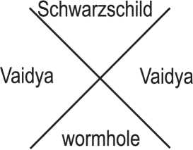
Figure 4: Matching domains: $\eta_{1}=\eta_{2}=1$ (left) and $\eta_{1}=\eta_{2}=-1$ (right).

In this subsection, we consider a collision of two oppositely moving impulses with Vaidya regions in opposite quadrants and Schwarzschild and static-wormhole regions in the other two quadrants. Connecting the impulses by (31) and (49), we find that $\eta_{1}=\eta_{2}=1$ if the future region is wormhole, and $\eta_{1}=\eta_{2}=-1$ if the future region is Schwarzschild (Fig.4). That is, $\eta_{1}=\eta_{2}$ in both cases. Then the constant $C$ is determined as

$$C=-\frac{M-m(V_{0})}{\sqrt{\lambda}}.$$ (50)

Here we implicitly use the fact that the jump of a jump vanishes, i.e. the jump across one impulse does not jump across the other impulse Jez .

IV Wormhole construction from Schwarzschild black hole

In this section we present analytic solutions which describe the construction of a static wormhole from a Schwarzschild black hole. The whole picture is represented by Fig. 5 and the strategy is as follows. Firstly, impulsive phantom radiation is beamed in, causing the trapping horizons to jump inward, much as a shell of normal matter makes a black-hole trapping horizon jump outward. By controlling the energy and timing of the impulses, the trapping horizons can be made to instantaneously coincide. They can then form the throat of a static wormhole if constant-profile streams of phantom radiation are beamed in subsequently, with the energy density appropriate to a wormhole of that area.

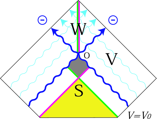
Figure 5: (Color online). Penrose diagram of the wormhole construction model. The wavy blue bold lines represent impulsive radiation with negative energy density. The region S is Schwarzschild, V is Vaidya and W is static-wormhole. The boundary between S and V corresponds to $z=0$ and the boundary between V and W corresponds to $z=l$.

IV.1 Vaidya region V

First, we set up an initial Schwarzschild region S (13) with mass $M$. Now we beam in impulsive phantom radiation symmetrically from either side, with the mass-energy of the shell being $\mu=4\pi r^{2}\sigma$, then turn on constant streams of phantom radiation immediately after the impulses. Then the region V should be Vaidya (16) with some mass function $m$, which on the boundary $V=V_{0}$ between S and V is

$$m(V_{0})=M-\eta\zeta\mu=M+\mu,$$ (51)

from the matching formula between Schwarzschild and Vaidya (III.1). Here we must take $\zeta=-1$ and $\eta=1$, since the impulse is ingoing into the black hole, and the radiation is the future of the Schwarzschild region.

In order for the final region W to be a static-wormhole region, the mass function $m$ of the Vaidya region V must take the following form;

$$m(z)=\frac{a}{2}(e^{-z^{2}}+2z\phi(z)-2\phi(z)^{2}e^{z^{2}})+C\phi(z)e^{z^{2}},$$ (52)

and the relation between the coordinates $V$ and $z$ is

$$V(z)=\int_{0}^{z}\frac{2a^{2}e^{-y^{2}}(e^{-y^{2}}+2y\phi(y))}{a\phi(y)-C}dy+V_{0}.$$ (53)

From Eqs. (51) and (52), $a$ is

$$a=2(M+\mu).$$ (54)

Connecting the impulsive radiation (31) and (49) at $l=0$, the constant $C$ is decided as

$$C=\frac{\mu}{\sqrt{\lambda}}.$$ (55)

IV.2 Wormhole region W

We consider the spacetime in the region W. Using the matching formula (46) between Vaidya (16) with the mass function (52) and a wormhole, we find that the region W is a static wormhole with the mass-energy

$$\epsilon(l)=(M+\mu)(e^{-l^{2}}+2l\phi(l)-2\phi(l)^{2}e^{l^{2}}).$$ (56)

The relation between the throat radius $r_{0}$ of the wormhole in the final region W and the Schwarzschild mass $M$ in the region S is

$$r_{0}=a=2M+2\mu.$$ (57)

Now we consider the energy and timing of the impulse. The tortoise coordinate $r^{\ast}$ inside a Schwarzschild black hole can be defined as

$$r^{\ast}=-r-2M\ln\left(1-\frac{r}{2M}\right)\qquad{\rm for}\quad r<2M,$$ (58)

so that $dr^{\ast}/dr>0$. In addition, the symmetry of the impulses means that the intersection point O is given by $t=0$, $r=r_{0}$ or $r^{\ast}=r^{\ast}_{0}$. Then the Eddington-Finkelstein relation (14) at the point O where the impulses collide gives

$$V_{0}=-r^{\ast}_{0}=2(M+\mu)+2M\ln\left(\frac{-\mu}{M}\right).$$ (59)

Thus the energy and timing of the impulses are related. From this relation, first, the energy of the impulses must be always negative, $\mu<0$. The throat radius of the final wormhole (57) must be less than the horizon radius of the initial Schwarzschild black hole. Second, the later the negative-energy impulses occur, the larger the absolute value of the energy of the impulses must be. These features are consistent with the results of the 2D model KHK .

In order for the final state not to have a naked singularity but to be a wormhole, the inequality $-M<\mu<0$ is required. The throat radius of the wormhole in the final region W must be smaller than the horizon radius of the initial black hole, $r_{0}<2M$, since $\mu$ must be negative. In summary, one can prescribe the initial black-hole mass $M>0$ and the impulse energy $\mu\in(-M,0)$ as free parameters, then the timing $V_{0}$ of the impulses and the throat radius $r_{0}$ of the final wormhole are determined.

V wormhole enlargement by impulsive radiation

In this section we present an analytic solution which represents the enlargement of a static wormhole. The whole picture is represented by Fig. 6 and the strategy is as follows. Basically we want to open then close an expanding region of past trapped surfaces, by moving apart then rejoining the two trapping horizons comprising the wormhole throat in W1. The general recipe is to first strengthen then weaken the negative energy density wh . This can be done with a two-shot combination of primary impulses with negative energy, followed by secondary impulses with positive energy. To make the situation analytically tractable, the constant-profile phantom radiation is turned off between the impulses, leaving the region S as Schwarzschild and the regions V1, V2 as Vaidya. By controlling the energy and timing of the impulses and the energy density of the final constant-profile radiation, the final region W2 is also a static wormhole, but larger.

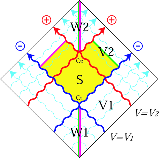
Figure 6: (Color online). Penrose diagram of the wormhole enlargement model. The wavy blue and red bold lines represent impulsive radiation with negative and positive energy density, respectively. The regions W1 and W2 are static-wormhole, V1 and V2 are Vaidya, and S is Schwarzschild. The boundary between W1 and V1 corresponds to $z=l$, the boundary between V1 and S corresponds to $z=0$, the boundary between S and V2 corresponds to $w=0$, and the boundary between V2 and W2 corresponds to $w=l$.

V.1 Vaidya region V1

We set up the initial region W1 as a static wormhole (6) with throat radius $r_{1}$. Then the gravitational energy $\epsilon_{1}$ is

$$\epsilon_{1}(l)=\frac{r_{1}}{2}(e^{-l^{2}}+2l\phi(l)-2\phi(l)^{2}e^{l^{2}}).$$ (60)

We beam in primary impulses symmetrically from both universes, then turn off the constant ghost radiation immediately after the impulses. Then the region V1 should be Vaidya. Timing the impulses at $V=V_{1}$, the matching formula (46) between static-wormhole and Vaidya regions yields the mass-energy $m_{1}$ in the region V1 as

$$m_{1}(z)=\frac{r_{1}}{2}(e^{-z^{2}}+2z\phi(z)-2\phi(z)^{2}e^{z^{2}})+C_{1}\phi(z)e^{z^{2}}$$ (61)

where the relation between the coordinates $V$ and $z$ is given by

$$V(z)=\int_{0}^{z}\frac{2r_{1}^{2}e^{-y^{2}}(e^{-y^{2}}+2y\phi(y))}{r_{1}\phi(y)-C_{1}}dy+V_{1}.$$ (62)

Connecting the impulsive radiation from the boundary between W and V1 to that between V1 and S, we can decide the constant $C_{1}=\mu_{1}/\sqrt{\lambda}$, where $\mu_{1}$ is the mass-energy of the primary impulses. Then the mass function of the first Vaidya region V1 at the boundary with Schwarzschild S becomes

$$m_{1}(z=0)=\frac{r_{1}}{2}$$ (63)

since the boundary surface $V=V_{1}$ coincides with $z=0$.

V.2 Schwarzschild region S

The region S is vacuum and therefore Schwarzschild. From the matching formula between Vaidya and Schwarzschild (III.1), the mass $M$ of the Schwarzschild region S becomes

$$M=\frac{r_{1}}{2}+\eta_{1}\zeta_{1}\mu_{1}=\frac{r_{1}}{2}-\zeta_{1}\mu_{1},$$ (64)

where $\eta_{1}=-1$, since the Vaidya region V1 is to the past of the Schwarzschild region S. Since we construct solvable symmetric models, the impulses are also both ingoing or outgoing. This means the region S must be inside a black-hole or white-hole region and $r_{1}<2M$. So when the impulse has negative energy, $\mu_{1}<0$, the sign of $\zeta_{1}$ must be positive,

$$M=\frac{r_{1}}{2}-\mu_{1}.$$ (65)

This means the radiation is outgoing,

$$\frac{dr}{dV}>0,$$ (66)

and S is a white-hole region. This is what we need to enlarge the wormhole, as a white-hole region is expanding. Conversely, one could reduce the wormhole size by taking $\mu_{1}>0$, creating a contracting black-hole region.

Now the symmetry of the impulses means that the intersection point $\rm O_{1}$ is given by $t=0$. Then the Eddington-Finkelstein relation (14) at the point $\rm O_{1}$ where the impulses collide gives

$$V_{1}=-r^{\ast}_{1}=r_{1}+2M\ln\left(1-\frac{r_{1}}{2M}\right)=2(M+\mu_{1})+2M\ln\left(\frac{-\mu_{1}}{M}\right).$$ (67)

Eqs. (64) and (67) mean that the timing $V_{0}$ of the impulses and the Schwarzschild mass $M$ are determined by the throat radius $r_{1}$ of the initial wormhole and the energy $\mu_{1}$ of the impulses.

V.3 Vaidya region V2

We next beam in secondary impulses symmetrically from both universes, and turn on constant-profile phantom radiation immediately after the impulses. Then the region V2 must be Vaidya. Timing the impulses at $V=V_{2}$, the matching formula between Vaidya and Schwarzschild (III.1) yields the mass function of the second Vaidya region V2 as

$$m_{2}(V_{2})=M-\eta_{2}\zeta_{2}\mu_{2}$$ (68)

on the boundary, where $\mu_{2}$ is the mass of the second shell. The region V2 is an outgoing Vaidya region which is to the future of the Schwarzschild region, so that $\eta_{2}=1$ and $\zeta_{2}=1$. Then

$$m_{2}(V_{2})=M-\mu_{2}=\frac{r_{1}}{2}-\mu_{1}-\mu_{2}.$$ (69)

Here in order for the final region W2 to be a static wormhole, the mass function $m_{2}$ must take the following form,

$$m_{2}(w)=\frac{1}{2}(r_{1}-2\mu_{1}-2\mu_{2})(e^{-w^{2}}+2w\phi(w)-2\phi(w)^{2}e^{w^{2}})+C_{2}\phi(w)e^{w^{2}},$$ (70)

where the coordinate $w$ is related with $V$ by

$$V(w)=\int_{0}^{w}\frac{2r_{2}^{2}e^{-y^{2}}(e^{-y^{2}}+2y\phi(y))}{r_{2}\phi(y)-C_{2}}dy+V_{2},$$ (71)

from the matching formula (45). Here $r_{2}$ is the throat radius of the wormhole in the final region W2. Connecting the impulsive radiation from the boundary between the regions S and V2 to that between V2 and W2, we can decide the constant $C_{2}=\mu_{2}/\sqrt{\lambda}$.

It can be shown that there are trapping horizons in the regions V2, as depicted in Fig 6; the negative-energy and positive-energy impulses respectively make the horizons jump to the future and the past. It is difficult to study the horizons analytically in the Vaidya coordinates, but it can be shown that they are null using dual-null coordinates $x^{\pm}$, as follows. If we have $V$ pointing along $x^{+}$, then there is only a $T_{++}$ component in the energy tensor. The $T_{--}$ and $T_{+-}$ components of the Einstein equations bhd then show respectively that, where $\partial_{-}r=0$, then $\partial_{-}\partial_{-}r=0$ and $\partial_{+}\partial_{-}r<0$, which means that the horizon $\partial_{-}r=0$ is null. Similar behavior occurs in the 2D model KHK , though the horizons were omitted in the corresponding diagram.

V.4 Wormhole region W2

Finally, we consider the spacetime in the region W2. Since constant-profile phantom radiation is beamed in for $V>V_{2}$ in order for the region V2 to be Vaidya (16) with the mass function (70), we can match it to a static-wormhole region from the matching formula (46). We find that the mass function $\epsilon_{2}$ of the wormhole in the region W2 is

$$\epsilon_{2}(l)=(r_{1}-2\mu_{1}-2\mu_{2})(e^{-l^{2}}+2l\phi(l)-2\phi(l)^{2}e^{l^{2}}),$$ (72)

and the throat radius $r_{2}$ is

$$r_{2}=r_{1}-2\mu_{1}-2\mu_{2}=2M-2\mu_{2}.$$ (73)

Again, the symmetry of the impulses means that the intersection point $\rm O_{2}$ is given by $t=0$. Then the Eddington-Finkelstein relation (14) at the point $\rm O_{2}$ where the impulses collide gives

$$V_{2}=-r^{\ast}_{2}=r_{2}+2M\ln\left(1-\frac{r_{2}}{2M}\right)=2(M+\mu_{2})+2M\ln\left(\frac{\mu_{2}}{M}\right).$$ (74)

From this relation, the energy of the impulses must be positive, $\mu_{2}>0$. In addition, the inequality

$$r_{2}>r_{1}$$ (75)

holds, since the region S is part of a white-hole region. That is, the wormhole is enlarged. We find that the absolute value $|\mu_{1}|$ of the energy density of the primary impulses should be stronger than that of the secondary impulses,

$$|\mu_{1}|>|\mu_{2}|$$ (76)

from Eqs. (73) and (75).

We find the relation between the energy and timing of impulses as

$$V_{2}-V_{1}=r^{\ast}_{2}-r^{\ast}_{1}=2(\mu_{1}+\mu_{2})+2M\ln\left(\frac{\mu_{2}}{-\mu_{1}}\right),$$ (77)

from Eqs. (67) and (74). Eq. (77) means that the longer the interval between the first and second impulses is, the smaller the value of energy density of the second impulse must be. In summary, once the throat radius of the initial wormhole and the energy of the impulses $(r_{1},\mu_{1},\mu_{2})$ are prescribed, the timings of the impulses, the intermediate Schwarzschild mass and the throat radius of the final wormhole $(V_{1},M,V_{2},r_{2})$ are determined. These features are also consistent with the results of the 2D model KHK .

VI jump in energy due to impulsive radiation

A general spherically symmetric metric can be written in dual-null form as

$$ds^{2}=r^{2}d\Omega^{2}-h\,dx^{+}dx^{-}$$ (78)

where $r\geq 0$ and $h>0$ are functions of the future-pointing null coordinates $(x^{+},x^{-})$. Writing $\partial_{\pm}=\partial/\partial x^{\pm}$, the propagation equations for the energy $E$ (1) are obtained from the Einstein equations as 1st

$$\partial_{\pm}E=8\pi h^{-1}r^{2}(T_{+-}\partial_{\pm}r-T_{\pm\pm}\partial_{\mp}r).$$ (79)

We have considered impulsive radiation defined by

$$T_{ab}=\frac{\mu_{\pm}\delta_{a}^{\pm}\delta_{b}^{\pm}}{4\pi r^{2}}\delta(x^{\pm}-x_{0})$$ (80)

where the constant $x_{0}$ gives the location of the impulse and the constant $\mu_{\pm}$ is its energy. More invariantly, the vector $\wp=-g^{-1}(\mu_{\pm}dx^{\pm})$ is the energy-momentum of the impulse. Then the jump

$$[E]_{\pm}=\lim_{\alpha\to 0}\int_{x_{0}-\alpha}^{x_{0}+\alpha}\partial_{\pm}E\,dx^{\pm}$$ (81)

in energy across the impulse is given by the jump formula

$$[E]_{\pm}=c^{\pm}\mu_{\pm},\qquad c^{\pm}=-2(h^{-1}\partial_{\mp}r)|_{x^{\pm}=x_{0}}.$$ (82)

The vector $c=c^{+}\partial_{+}+c^{-}\partial_{-}$ is actually $c=g^{-1}(dr)$ and so

$$[E]_{\pm}=-\wp\cdot dr$$ (83)

is a manifestly invariant form of the jump formula. Note that while the energy-momentum vector $\wp$ (or $\mu_{\pm}dx^{\pm}$) is invariant, the energy $\mu_{\pm}$ depends on the choice of null coordinate $x^{\pm}$, reflecting the fact that a particle moving at light-speed has no rest frame and no preferred energy. However, in a curved but stationary space-time, the stationary Killing vector provides a preferred frame and a preferred energy $\mu_{\pm}$.

We need only employ the jump formula in the following cases. (i) Inside a Schwarzschild black hole, we can take future-pointing $x^{\pm}=-r^{\ast}\pm t$ where $dr^{\ast}/dr=(2M/r-1)^{-1}$. Then $r^{\ast}=-(x^{+}+x^{-})/2$, $h=2M/r-1$ and $\partial_{\pm}r=(dr/dr^{\ast})\partial_{\pm}r^{\ast}=(1-2M/r)/2$ gives $c^{\pm}=1$ and $[E]_{\pm}=\mu_{\pm}$. (ii) Inside a Schwarzschild white hole, we can take future-pointing $x^{\pm}=r^{\ast}\pm t$ and similarly obtain $c^{\pm}=-1$ and $[E]_{\pm}=-\mu_{\pm}$. (iii) On the throat of a static wormhole, where $\partial_{+}r=\partial_{-}r=0$ and $h$ is finite MT , one finds $c^{\pm}=0$ and $[E]_{\pm}=0$. This is summarized as

$$[E]_{\pm}=\left\{\begin{array}[]{ll}\mu&\quad\hbox{inside a Schwarzschild black hole}\\ -\mu&\quad\hbox{inside a Schwarzschild white hole}\\ 0&\quad\hbox{on the throat of a static wormhole}\end{array}\right.$$ (84)

where the indices on $\mu_{\pm}$ are now omitted.

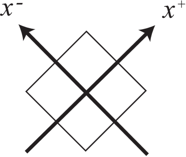
Figure 7: an infinitesimal box across which two radiative impulses (arrows) intersect.

Now assuming an infinitesimal diamond-shaped box around the point where the impulses collide as in Fig.7, we can evaluate the jump in energy across the impulses for each case in Secs. IV and V. For wormhole construction (Fig.5), the energy $E$ will jump by $\mu$ from the region S to V and by $0$ from the region V to W, evaluated in the limit at the point, recovering $r_{0}/2=M+\mu$ (57), where $M$ is the black-hole mass in the region S. Similarly for wormhole enlargement (Fig.6), the energy $E$ will jump by $0$ from W1 to V1 and by $-\mu_{1}$ from V1 to S at the point $\rm O_{1}$, and by $-\mu_{2}$ from the region S to V2 and by $0$ from the region V2 to W2 at $\rm O_{2}$, recovering $M=r_{1}/2-\mu_{1}$ (65) and $r_{2}/2=M-\mu_{2}$ (73), where $M$ is the black-hole mass in the region S.

Thus even without performing the detailed matching, the basic properties of the solutions could be predicted simply by the jump formula for $E$ and continuity of the area $A=4\pi r^{2}$. For wormhole construction, continuity of $r$ at O implies $r_{0}<2M$, and the jump formula gives $\mu<0$; the impulses must have negative energy. Similarly, for wormhole enlargement, continuity of $r$ at O1 and O2 implies $r_{1}<2M$ and $r_{2}<2M$, and the jump formula gives $\mu_{1}<0$ and $\mu_{2}>0$; the primary and secondary impulses must have negative and positive energy respectively.

VII Summary

In this paper, we have studied wormhole dynamics in Einstein gravity under (phantom and normal, impulsive and regular) pure radiation, constructing analytic solutions where a traversable wormhole is created from a black hole, or the throat area of a traversable wormhole is enlarged or reduced, the size being controlled by the energy and timing of the impulses. The solutions are composed of Schwarzschild, static-wormhole pr and Vaidya regions matched across null boundaries according to the Barrabès-Israel formalism. For this purpose we have derived the matching formulas which apply when the direction of radiation in the Vaidya region is either parallel or transverse to the boundary. These formulas are useful for other problems.

The results provide concrete examples of how to create and enlarge traversable wormholes, given the existence of Schwarzschild black holes and phantom energy. We have worked within standard General Relativity, inventing no new theoretical physics other than an idealized model of phantom energy, on which general arguments do not depend wh . Thus if space-time foam and phantom energy do exist and can be controlled, then traversable wormholes can be constructed and enlarged.

- (1) M.S. Morris & K.S. Thorne, Am. J. Phys. 56, 395 (1988).
- (2) M. Visser, Lorentzian Wormholes: from Einstein to Hawking (AIP Press 1995).
- (3) D.N. Spergel et al., Astroph. J. Suppl. 148, 175 (2003).
- (4) L.M. Krauss, Astroph. J. 596, L1 (2003).
- (5) R.R. Caldwell, Phys. Lett. B545, 23 (2002).
- (6) D. Hochberg & M. Visser, Phys. Rev. D58, 044021 (1998).
- (7) D. Hochberg & M. Visser, Phys. Rev. Lett. 81, 746 (1998).
- (8) S.A. Hayward, Int. J. Mod. Phys. D8, 373 (1999).
- (9) D. Ida & S. A. Hayward, Phys. Lett. A260, 175 (1999).
- (10) S.A. Hayward, Phys. Rev. D49, 6467 (1994).
- (11) S.A. Hayward, Class. Quantum Grav. 15, 3147 (1998).
- (12) S.A. Hayward, S-W. Kim & H. Lee, Phys. Rev. D65, 064003 (2002).
- (13) H. Shinkai & S.A. Hayward, Phys. Rev. D66, 044005 (2002).
- (14) S.A. Hayward, Phys. Rev. D65, 124016 (2002).
- (15) H. Koyama, S.A. Hayward & S-W. Kim, Phys. Rev. D67, 084008 (2003).
- (16) C. Barrabès & W. Israel, Phys. Rev. D43, 1129 (1991).
- (17) P.C. Vaidya, Proc. Indian Acad. Sci., Sect. A33, 264 (1951).
- (18) J.A. Wheeler, Ann. Phys. 2, 604 (1957).
- (19) S.A. Hayward & H. Koyama, How to make a traversable wormhole from a Schwarzschild black hole (gr-qc/0406080).
- (20) C.W. Misner & D.H. Sharp, Phys. Rev. 136, B571 (1964).
- (21) S.A. Hayward, Phys. Rev. D53, 1938 (1996).
- (22) H.G. Ellis, J. Math. Phys. 14, 104 (1973).
- (23) L.A. Gergely, Phys. Rev. D58, 084030 (1998).
- (24) J. Jezierski, J. Math. Phys. 44, 641 (2003).