Differing Calculations of the Response of Matter-wave Interferometers to Gravitational Waves

Abstract

There now exists in the literature two different expressions for the phase shift of a matter-wave interferometer caused by the passage of a gravitation wave. The first, a commonly accepted expression that was first derived in the 1970s, is based on the traditional geodesic equation of motion (EOM) for a test particle. The second, a more recently derived expression, is based on the geodesic deviation EOM. The power-law dependence on the frequency of the gravitational wave for both expressions for the phase shift is different, which indicates fundamental differences in the physics on which these calculations are based. Here we compare the two approaches by presenting a series of side-by-side calculations of the phase shift for one specific matter-wave-interferometer configuration that uses atoms as the interfering particle. By looking at the low-frequency limit of the different expressions for the phase shift obtained, we find that the phase shift calculated via the geodesic deviation EOM is correct, and the ones calculated via the geodesic EOM are not.

I Introduction

In two recent papers nmMIGO (2003); CrysMIGO (2003), a new calculation of the phase shift of a matter-wave interferometer caused by the passage of a gravitational wave was presented. This calculation was based not on the usual geodesic equation of motion (EOM), but rather on the geodesic deviation EOM. Contrary to expectations, these phase shifts have a form that is very much different from those calculated previously in the literature Linet-Tourrenc (1976); Stodolsky (1979); Papini (1989); Borde1 (1994); Borde2 (1997); Borde3 (2001); Alsing (2001). While a direct comparison of the various expressions for the phase shift is difficult because of the different configurations of the matter-wave interferometers used for their calculations, it was noted in nmMIGO (2003) that the power-law dependence on the frequency of the gravitational wave, in both the low- and high-frequency limit, of the expressions calculated in nmMIGO (2003); CrysMIGO (2003) are at times diametrically opposite to those calculated in Linet-Tourrenc (1976); Stodolsky (1979); Papini (1989); Borde1 (1994); Borde2 (1997); Borde3 (2001); Alsing (2001). Consequently, we expect that the differences between these expressions are not due simply to differences in the configurations of the interferometers chosen, but are rather caused by fundamental differences in the physics on which their derivations are based.

In this paper our objective is to demonstrate that these fundamental differences do exist by presenting a series of calculations that follows the two basic approaches in the literature used to determine the phase shift caused by a gravitational wave. This will be done for the same configuration of matter-wave interferometer, and will allow us to compare the different expressions we obtain for the phase shift on an equal footing. We then determine their validity by comparing each of them, in the appropriate limit, with the well-known expression for the phase shift caused by stationary sources of spacetime curvature Anandan (1979); Chiao (2003); Papini (1989). The focus in this paper will be on a theoretical study of the underlying physics; we leave issues of the practicality and feasibility of constructing the interferometer to nmMIGO (2003); CrysMIGO (2003).

The various approaches taken to determine the phase shift of a matter-wave interferometer caused by a gravitational wave can be divided into two distinctly separate classes. The class of approaches that is more often found in the literature Linet-Tourrenc (1976); Stodolsky (1979); Papini (1989); Borde1 (1994); Borde2 (1997); Borde3 (2001); Alsing (2001) is done in transverse-traceless (TT) coordinates (see Sec. 9.2.3 of Thorne (1987)), either explicitly or implicitly. The TT coordinates are one specific choice of reference frame where the gravitation wave is in the TT gauge. In this frame the number of components of the deviations of the flat spacetime metric $h_{\mu\nu}$ caused by the gravitational wave equals the number of physical degrees of freedom of the gravitational wave. Consequently, $\partial^{\mu}h_{\mu\nu}$, $h_{0\mu}=0$, and $h_{\mu}^{\mu}=0$. In addition, the mirrors and the beam splitters are at fixed coordinate values in these coordinates, and they do not move. These coordinates have been used to study the properties of light-wave-interferometry-based detectors of gravitational waves as well Hellings (1983). To calculate the phase shift for matter-wave interferometers, it is combined with either the geodesic EOM (and its action), if the calculation is done at the quantum-mechanical level Linet-Tourrenc (1976); Alsing (2001), or the Lagrangian (and the WKB or stationary phase approximation) for a quantum field in curved spacetime, if the calculation is done at the quantum field-theoretic level Papini (1989); Borde1 (1994); Borde2 (1997); Borde3 (2001). Not surprisingly, irrespective of the level of sophistication of the approach used, the general expressions calculated for the phase shift have the same final form.

The other class of approaches to calculating the phase shift is taken by nmMIGO (2003); CrysMIGO (2003), and is done in Thorne’s “proper reference frame”. They follow the classical analysis in Thorne (1987); Thorne1983 (1983); Misner et al. (1973) for light-wave-based interferometers. In this frame, the positions and velocities of test particles are measured relative to the worldline of an observer, and follow the motion of the observer in spacetime, in much the same way that the Fermi-normal Fermi , Fermi-Walker coordinates Synge (1960), and the recently constructed general laboratory frame general laboratory frame (2003) do. Consequently, the motion of the test particle in this frame is not described by the usual geodesic equation of motion (EOM), but rather by the geodesic deviation EOM (see Eq. (2) of Thorne (1987)), which was first applied to the analysis of physical systems in Synge (1926); Levi-Civita (1926). As in Thorne (1987), the TT gauge was taken for the gravitational wave. The action (see Synge (1935); Speliotopoulos (1995); general laboratory frame (2003)) for the geodesic deviation EOM was then used in conjunction with the quasi-classical approximation of the Feynman-path-integral formulation of quantum mechanics. This approximation is the Lagrangian form of the WKB approximation in the Schrödinger representation of quantum mechanics, and in nmMIGO (2003); CrysMIGO (2003) it was applied to the calculation of the phase shift of the two matter-wave-interferometer configurations.

The phase shift of a matter-wave interferometer is a physically measurable quantity. From the principle of general covariance, it should not matter whether the TT coordinates, or whether the proper reference frame is used in its calculation Thorne (1987); Unruh-Weiss . Indeed, Thorne states the following:

“If $L<<\lambdabar$ then the [gravitational wave] detector can be contained entirely in the proper reference frame of its center, and the analysis can be performed using non-relativistic concepts augmented by the quadrupolar gravity-wave force field (3), (5). If one prefers, of course, one instead can analyze the detector in TT coordinates using general relativistic concepts and the spacetime metric (8). The two analyses are guaranteed to give the same predictions for the detector’s performance, unless errors are made [emphasis added].” (From page 400 of Thorne (1987).)

Evidently, errors have indeed been made, as we shall see, since the resulting calculations often contradict each other for the same interferometer. The power-law dependence on frequency of the phase shifts calculated in Linet-Tourrenc (1976); Stodolsky (1979); Papini (1989); Borde1 (1994); Borde2 (1997); Borde3 (2001); Alsing (2001) using TT coordinates are fundamentally different from that of the phase shifts calculated in nmMIGO (2003); CrysMIGO (2003) using the proper reference frame. Since the principle of general covariance must hold, this means that either (a) the calculations in nmMIGO (2003); CrysMIGO (2003) are wrong, (b) the calculations in Linet-Tourrenc (1976); Stodolsky (1979); Papini (1989); Borde1 (1994); Borde2 (1997); Borde3 (2001); Alsing (2001) are wrong, or (c) all of the calculations of the phase shifts are wrong.

To determine which one of these three possibilities is correct, we will present side by side calculations of the phase shift caused by a gravitational wave for one specific matter-wave-interferometer configuration using the following three approaches. The first calculation uses the quasi-classical approximation in the TT coordinates and geodesic action, and is done at the nonrelativistic, quantum-mechanics level. It follows, as much as possible, the line of analysis given in Stodolsky (1979). The second calculation is also done at the nonrelativistic, quantum-mechanics level using the same approximation, but now in the proper reference frame, and uses the geodesic deviation action. It follows the line of analysis given in nmMIGO (2003).

These two calculations would seem to exhaust the two different classes of approaches currently found in the literature. That a third calculation of the phase shift is needed is because of an error in Linet-Tourrenc (1976); Stodolsky (1979); Papini (1989); Borde1 (1994); Borde2 (1997); Borde3 (2001); Alsing (2001). Either because changes in the kinetic energy term in the action for the atom in Stodolsky (1979); Alsing (2001) were neglected, or because the turning points of the atom’s phase at the interferometer’s mirrors in the WKB-type of approach in Linet-Tourrenc (1976); Papini (1989); Borde1 (1994); Borde2 (1997); Borde3 (2001) were omitted, the end result is that important boundary terms are not included in the final expression for the phase shift in Linet-Tourrenc (1976); Stodolsky (1979); Papini (1989); Borde1 (1994); Borde2 (1997); Borde3 (2001); Alsing (2001). For the sake of completeness, and to compare the calculations in nmMIGO (2003); CrysMIGO (2003) with these previous calculations in the literature, this necessitates a third calculation of the phase shift, which will result in yet another expression for the phase shift based on the geodesic EOM.

We find that all three expressions for the phase shift calculated here are different from one another. Although there are currently no direct experimental checks that can used to determine which one of these three expressions for the phase shift is correct, an indirect experimental check can be used by taking the low-frequency limit.

All three expressions for the phase shift depend on the transit time of the atom through the interferometer, and the period of the gravitational wave. If the transit time of the atom is much shorter than the period, then, with respect to the atom, the gravitational wave does not oscillate appreciably as it traverses the interferometer. The gravitational wave will contribute a local Riemannian curvature to the spacetime that is effectively static. The phase shift of matter-interferometers caused by static (as well as stationary) sources of curvature is well established Anandan (1979); Chiao (2003); Papini (1989), and has been shown to be proportional to components of the Riemann curvature tensor. Just as importantly, this phase shift can be calculated using only Newtonian gravity [Eq. (2.6) of Anandan (1979)]. The phase shift due to the Newtonian gravitational potential—through the acceleration due to Earth’s gravity $g$—has been measured, first by Collela, Overhauser and Werner COW , and more recently by Chu and Kasevich ChuKas . These more recent measurements of the phase shift induced by $g$ are sensitive enough that effect of spatial variations in $g$—which are proportional to the static Riemann curvature of the spacetime caused by the Earth—on the phase shift can be discerned. Gradients in $g$ were seen through changes in the phase shift of an atomic fountain when its vertical position was varied PCC . More recently, they were seen through a differential measurement of the phase shifts of two atomic fountain matter-wave interferometers operating in tandem Kas . Therefore, while the direct measurement of the phase shift of a matter-wave interferometer caused by a static Riemann curvature tensor has not been made, its discovery is expected. Indeed, indications are that the phase shift induced by the static Riemann curvature of the Earth has already been seen PrivateKas .

As a consequence of the above, in the limit of low-frequency gravitational waves the phase shift calculated for the matter-wave interferometer must approach the well-known static result, and be proportional to the curvature tensor. We will see that in this limit, only the phase shift calculated along the lines of nmMIGO (2003); CrysMIGO (2003) has the correct form. The other two do not, and must be wrong, since they do not yield the correct static limit.

Our focus here is on the phase shift that a gravitational wave will induce on a matter-wave interferometer. We will thus neglect the effects of all other gravitational effects—such as the acceleration due to Earth’s gravity, and the local curvature of spacetime due to stationary sources such as the Earth, Sun and Moon—in addition to the phase shift due to the Sagnac effect caused by the Earth’s rotation. We have shown in general laboratory frame (2003) that for these types of stationary gravitational effects the description of the motion of test particles in the general laboratory frame—of which the proper reference frame is a special case—reduces to the usual geodesic EOM description, and there is no controversy. The phase shifts caused by these stationary effects calculated in either the proper reference frame or the TT coordinates will be the same.

We will in this paper use the same notation the is commonly found in the literature nmMIGO (2003); CrysMIGO (2003); Linet-Tourrenc (1976); Stodolsky (1979); Papini (1989); Borde1 (1994); Borde2 (1997); Borde3 (2001); Alsing (2001). In particular, it follows the notation in Thorne (1987). While this has the benefit of consistency and simplicity, it means that we do not separate with notation the coordinates used for the TT coordinates from the coordinate used for the proper reference frame. The coordinates used in the two reference frames have different physical meanings, which we will make clear in the next section. These differences are outlined in detail in general laboratory frame (2003).

II Phase-Shift Calculations

In this section we will present two of the three calculations of the phase shift mentioned in the introduction. The first calculation will be done in the TT coordinates, and will be based on the geodesic EOM. The second calculation will be done in the proper reference frame, and will be based on the geodesic deviation EOM. A third calculation, following the approach in the literature, will be done in the next section where comparisons between the different results of the calculations are made. All three calculations are done for gravitational waves in the long-wavelength limit for the matter-wave interferometer configuration shown in Fig. 1; this configuration is described in detail in appendix A. To calculate the phase shifts, we will use the quasi-classical approximation of the Feynman path integral representation of quantum mechanics. This approximation is the Lagrangian version of the WKB approximation, or stationary phase approximation, in the Schrödinger representation of quantum mechanics, and will be reviewed in appendix A as well. The presentation in this section is done in detail to ensure that all the underlying assumptions, approximations, and subtleties in our analysis are readily apparent.

II.1 Geodesic-EOM-based calculation of the phase shift

II.1.1 Classical Dynamics in TT Coordinates

Consider a gravitational wave in the long-wavelength limit with an amplitude $h_{\mu\nu}(t)$ incident perpendicularly to the plane of the interferometer in Fig. 1. As usual, Greek indices run from $0$ to $4$, and Latin indices run from $1$ to $3$. The gravitational wave is represented by the tensor $h_{\mu\nu}$ as a perturbation on the flat spacetime metric $\eta_{\mu\nu}$, so that the total metric of the spacetime is $g_{\mu\nu}=\eta_{\mu\nu}+h_{\mu\nu}$. We have chosen the signature of $g_{\mu\nu}$ to be $(-1,1,1,1)$. In the TT-gauge, a coordinate system is chosen so that in these coordinates, $\partial^{\mu}h_{\mu\nu}=0$, $h_{0\mu}=0$, and $h_{\mu}^{\mu}=0$; the only nonvanishing components of $h_{\mu\nu}$ are thus $h_{ij}$.

One choice of coordinates where the TT gauge is realized is the TT coordinates (see Thorne (1987) and the general analysis in Wald ). In these coordinates the action for the atom with mass $m$ used in Fig. 1 is the usual geodesic action in the nonrelativistic limit,

$$S_{geo}=-m\int\left(-\frac{dx^{\mu}}{dt}\frac{dx^{\nu}}{dt}g_{\mu\nu}\right)^{1/2}dt\approx-mc^{2}t+\frac{1}{2}m\int\left[v^{i}v^{j}(\delta_{ij}+h_{ij})\right]dt,$$ (1)

where the subscript “geo” stands for “geodesic”. Since the rest mass $mc^{2}$ only shifts the Lagrangian for the atom by a constant, we drop this term from $S_{geo}$. The nonrelativistic Hamiltonian for the motion is then,

$$H_{geo}=\frac{\vec{p}^{\>2}}{2m}-\frac{1}{2m}p^{i}p^{j}h_{ij},$$ (2)

which results in the usual geodesic equation of motion

$$\frac{d^{2}x^{i}}{dt^{2}}=-2\Gamma^{i}_{0j}\frac{dx^{j}}{dt}=-\dot{h}^{i}_{j}\frac{dx^{j}}{dt}.$$ (3)

Here $\Gamma^{\alpha}_{\mu\nu}$ is Christoffel symbol for the spacetime; for gravitational waves in the TT gauge, $\Gamma^{i}_{0j}=\dot{h}^{i}_{j}/2$.

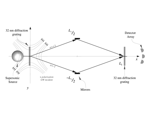
Figure 1: Schematic of the matter-wave interferometer configuration considered in this paper with a gravitational wave incident normal to the plane of the interferometer shown. Only the $\times$ polarization contributes to the phase shift; the $+$ polarization does not. Diffraction orders other than $n=\pm 1$ are not used, and are left out for clarity.

To calculate the phase shift of Fig. 1, we follow the description in appendix A, and consider the phase shift due to the $r$th atom emitted from the atomic source, which at a time $t_{r}$ is diffracted by the initial beam splitter. There are two possible classical paths for the atom through the interferometer. In the absence of gravitational waves, these are straight-line paths $\vec{x}_{0}(t)$ (see appendix A), which will be shifted when a gravitational wave is present. These shifts are expected to be very small, however, and we can use perturbation theory to solve for them. We thus take $\vec{x}(t)=\vec{x}_{0}(t)+\vec{x}_{1}(t)$, and $\vec{v}(t)=\vec{v}_{0}(t)+\vec{v}_{1}(t)$, where $\vec{x}_{1}(t)$ and $\vec{v}_{1}(t)$ are perturbations to the atom’s path $\vec{x}_{0}(t)$ and velocity $\vec{v}_{0}(t)$, respectively; we will keep only terms linear in $\vec{v}_{1}(t)$. To first order in $h_{ij}$, Eq. $(\ref{geoeqn})$ becomes

$$\frac{dv_{1}^{i}}{dt}=-\dot{h}^{i}_{j}v_{0}^{j}.$$ (4)

Once $\vec{x}_{0}(t)$ is determined, $v_{1}(t)$ is solved for by dividing the trajectory of an atom into two parts: from the initial beam splitter to the mirror, and then from the mirror to the final beam splitter. The two paths are then joined with the appropriate boundary conditions at the mirror.

We begin by determining $\vec{x}_{0}(t)$.

II.1.2 Trajectories in the absence of gravitational waves

To determine the unperturbed path of the atoms through the interferometer—which is the same no matter which approach is used to calculate the phase shifts—consider first the path of the atom that is diffracted into the $n=+1$ diffraction order. We will assume that the velocity of the atoms is high enough that we can ignore the effect of Earth’s gravity on the atom. It is then clear that for $t_{r}<t<t_{r}+T/2$—during which it travels between the initial beam splitter and the first mirror in a time $T/2$—the path of the atom is

$$v_{0x}=v_{\|}, x_{0}(t)=v_{\|}(t-t_{r}),$$

$$v_{0y}=v_{\bot}, y_{0}(t)=v_{\bot}(t-t_{r}),$$ (5)

where $v_{\|}$ and $v_{\bot}$ are $x$ and $y$ components of the velocity of the atom immediately after it leaves the initial beam splitter. At $t_{r}+T/2$ the atom is reflected off the hard-wall mirror, and from the general expression of the boundary condition for the atom at the mirror Eq. $(\ref{bc})$, $v_{0x}(t_{r}+T^{+}/2)=v_{0x}(t_{r}+T^{-}/2)=v_{\|}$, while $v_{0y}(t_{r}+T^{+}/2)=-v_{0y}(t_{r}+T^{-}/2)=-v_{\bot}$. (The superscripts $\pm$ denote $\lim_{\epsilon\to 0}t_{r}+T/2\pm\epsilon$ respectively.) For the subsequent time interval $t_{r}+T/2<t<t_{r}+T$, the atom’s path is

$$v_{0x}=v_{\|}, x_{0}(t)=v_{\|}(t-t_{r}),$$

$$v_{0y}=-v_{\bot}, y_{0}(t)=L_{\bot}-v_{\bot}(t-t_{r}),$$ (6)

during which it travels between the mirror and the final beam splitter. It is clear that $L_{\bot}=v_{\bot}T$ and $L_{\|}=v_{\|}T$, and $T$ is the total transit time of the atom through the interferometer. The unperturbed path for the atom in the $n=-1$ diffraction order is similar to Eqs. $(\ref{firsthalf})$ and $(\ref{secondhalf})$, and is obtained by taking $v_{\bot}\to-v_{\bot}$ and $L_{\bot}\to-L_{\bot}$.

II.1.3 Boundary conditions

To determine the boundary conditions for $\vec{v}_{1}$ in Eq. $(\ref{pert-geo})$, we note that from Eq. $(\ref{geoeqn})$ the acceleration of a test particle for the geodesic EOM is proportional to its velocity. As such, a test particle which was initially at rest will stay at rest, even in the presence of a gravitational wave. This led to the following conclusion by Stodolsky:

“In this discussion [of matter-wave interferometry] we have assumed that the parts of the apparatus [interferometer] stay at fixed coordinate values. This can be achieved if these parts are free masses, since a metric of the gravity wave type (with no “0” components) does not affect the positions of nonmoving bodies.” (From page 399 of Stodolsky (1979).)

Thus, in the TT coordinates, the positions of beam splitters and the mirrors do not change when a gravitational wave passes through the system.

The velocity of the atoms travelling between the supersonic source and the initial beam splitter, on the other hand, will be affected by the gravitational wave. Since the interferometer in Fig. 1 is balanced, only differences in the atom’s trajectory along the two paths through it will matter. We can thus neglect any shifts in the atom’s velocity before it reaches the beam splitter. And, since the initial beam splitter is not moved by the gravitational wave, $v_{0x}(t_{r})=v_{\|}$ while $v_{0y}(t_{r})=v_{\bot}$; thus we take $\vec{v}_{1}(t_{r})=0$.

For the boundary conditions at the mirror, we note that like the beam splitter, the positions of the mirrors in the interferometer also do not change when a gravitational wave is present. Thus the boundary conditions for $\vec{v}_{1}(t)$ across the hard-wall mirrors is

$$v_{1x}(t_{r}+T^{+}/2)=v_{1x}(t_{r}+T^{-}/2),\qquad v_{1y}(t_{r}+T^{+}/2)=-v_{1y}(t_{r}+T^{-}/2).$$ (7)

Integrating Eq. $(\ref{pert-geo})$ is now straightforward, and for $t_{r}<t<t_{r}+T/2$,

$$v_{1x}(t) = -v_{\|}h_{xx}(t)-v_{\bot}h_{xy}(t)+v_{\|}h_{xx}(t_{r})+v_{\bot}h_{xy}(t_{r}),$$

$$v_{1y}(t) = -v_{\|}h_{xy}(t)-v_{\bot}h_{yy}(t)+v_{\|}h_{xy}(t_{r})+v_{\bot}h_{yy}(t_{r}),$$ (8)

while for $t_{r}+T/2<t<t_{r}+T$,

$$v_{1x}(t) = -v_{\|}h_{xx}(t)+v_{\bot}h_{xy}(t)+v_{\|}h_{xx}(t_{r})-2v_{\bot}h_{xy}(t_{r}+T/2)+v_{\bot}h_{xy}(t_{r}),$$

$$v_{1y}(t) = -v_{\|}h_{xy}(t)+v_{\bot}h_{yy}(t)-v_{\|}h_{xy}(t_{r})+2v_{\|}h_{xy}(t_{r}+T/2)-v_{\bot}h_{yy}(t_{r}).$$ (9)

II.1.4 The phase shift

We now calculate the action for the $r$th atom as it travels through along the upper path through the interferometer. To first order in $h_{ij}$,

$$S_{geo}^{cl}[\vec{x}(t_{r}),\vec{x}(t_{r}+T);\gamma_{+1}] \equiv \frac{1}{2}m\int_{t_{r}}^{t_{r}+T}\left\{[\vec{v}_{0}(t)+\vec{v}_{1}(t)]^{2}+v_{0}^{i}v_{0}^{j}h_{ij}\right\}dt,$$ (10)

$$\approx \frac{1}{2}m\int_{t_{r}}^{t_{r}+T}\vec{v}_{0}^{\>2}\>dt+m\int_{t_{r}}^{t_{r}+T}\left\{\vec{v}_{0}\cdot\vec{v}_{1}(t)+\frac{1}{2}v_{0}^{i}v_{0}^{j}h_{ij}\right\}dt,$$

where the superscript “cl” stands for “classical”, and denotes that the integration is over a classical path through the interferometer. The $\vec{v}_{0}^{\>2}$ term in Eq. $(\ref{ActionGeo})$ is the same for both paths through the interferometer, and will not contribute to the phase shift. It can be neglected. The last term $v_{0}^{i}v_{0}^{j}h_{ij}$ can be trivially integrated using Eqs. $(\ref{firsthalf})$ and $(\ref{secondhalf})$, while the $\vec{v}_{0}\cdot\vec{v}_{1}$ term can be integrated using Eqs. $(\ref{geosolutions-first})$ and $(\ref{geosolutions-second})$. We then get

$$\tilde{S}^{geo}_{cl}[\vec{x}(t_{r}),\vec{x}(t_{r}+T);\gamma_{+1}]= T\left[v_{\|}^{2}h_{xx}(t_{r})+v_{\bot}^{2}h_{yy}(t_{r})\right]$$

$$-\frac{1}{2}\int_{t_{r}}^{t_{r}+T}\bigg{[}v_{\|}^{2}h_{xx}(t)+v_{\bot}^{2}h_{yy}(t)\bigg{]}dt$$

$$+2v_{\bot}v_{\|}T\bigg{[}h_{xy}(t_{r})-h_{xy}(t_{r}+T/2)\bigg{]}$$

$$-v_{\bot}v_{\|}\left(\int_{t_{r}}^{t_{r}+T/2}h_{xy}(t)\>dt-\int_{t_{r}+T/2}^{t_{r}+T}h_{xy}(t)\>dt\right),$$ (11)

where the tilde denotes the fact that we have dropped the $\vec{v}^{\>2}$ term from the action. We get the action $\tilde{S}_{geo}^{cl}[\vec{x}(t_{r}),\vec{x}(t_{r}+T);\gamma_{-1}]$ for the atom if it took the lower path through the interferometer by taking $v_{\bot}\to-v_{\bot}$ in $\tilde{S}_{geo}^{cl}[\vec{x}(t_{r}),\vec{x}(t_{r}+T);\gamma_{+1}]$. The first two terms in Eq. $(\ref{ActionGeoFinal})$ do not change, while the last two terms flip sign. Thus, from Eq. $(\ref{def-phase-shift})$, the phase shift of the atom is

$$\Delta\phi_{geo}(t_{r})=-\frac{2m}{\hbar}L_{\|}L_{\bot} \Bigg{\{}2\left[\frac{h_{xy}(t_{r}+T/2)-h_{xy}(t_{r})}{T}\right]$$

$$+\frac{1}{T^{2}}\left(\int_{t_{r}}^{t_{r}+T/2}h_{xy}(t)\>dt-\int_{t_{r}+T/2}^{t_{r}+T}h_{xy}(t)\>dt\right)\Bigg{\}}.$$ (12)

After taking the Fourier transform,

$$h_{xy}(t)\equiv\int_{-\infty}^{\infty}\frac{d\omega}{2\pi}h_{\times}(\omega)e^{-i\omega t},\qquad\Delta\phi_{geo}(t)\equiv\int_{-\infty}^{\infty}\frac{d\omega}{2\pi}\Delta\phi_{geo}(\omega)e^{-i\omega t},$$ (13)

the calculated phase shift for Fig. 1 using TT coordinates simplifies to

$$\Delta\phi_{geo}(\omega)\equiv -\frac{m}{2\hbar}L_{\|}L_{\bot}i\omega h_{\times}(\omega)e^{-i\omega T/2}F_{geo}(\omega T),$$

$$F_{geo}(\omega T)= \bigg{[}\hbox{sinc}\,(\omega T/4)\bigg{]}^{2}-4e^{i\omega T/4}\hbox{sinc}\,(\omega T/4),$$ (14)

where $\hbox{sinc}\,(x)=\sin(x)/x$. The first result of our comparison of phase-shift calculations for the interferometer shown in Fig. 1 is given in Eq. $(\ref{PhaseGeoRes})$. The derivation of these equations is based on the geodesic equation of motion using the TT coordinates. We will find that the phase shift calculated in all three approaches in this paper will have this same overall form, and will differ only in the resonance function $F_{geo}$.

II.2 Geodesic-deviation-EOM-based calculation of the phase shift

Reference frames centered on the worldline of an observer, such as the proper reference frame and general laboratory frame, are less commonly used than the TT coordinates used in the previous subsection. We therefore begin the calculation of the phase shift for Fig. 1 in the proper reference frame with a brief review of this frame.

II.2.1 The proper reference frame

How the proper reference frame is constructed is described as follows:

“Consider an observer (freely falling or accelerated, it doesn’t matter so long as the acceleration is slowly varying). Let the observer carry with herself a small Cartesian latticework of measuring rods and synchronized clocks (a ‘proper reference frame’ in the sense of Sec. 13.6 of MTW, with spatial coordinates $x^{j}$ that measure proper distance along orthogonal axes).” (From page 339 of Thorne (1987).)

In this frame the coordinate $x^{i}(t)$ is the position of a nonrelativistic test particle travelling along its worldline relative to the worldline of the observer at her propertime $t$. The magnitude of $x^{i}(t)$ is then the distance between the worldline of the test particle, and the worldline of the observer at the same instant of time $t$. This frame is only valid when the test particle is moving nonrelativistically, and the size of the apparatus is small compared to the wavelength of the gravitational wave. The velocity $v^{i}(t)=\dot{x}^{i}$ is then the velocity of the test particle measured relative to the observer.

In the absence of all other forces, both the test particle and the observer travel along geodesics in the spacetime, and thus their motion are each, separately, governed by geodesic EOMs. By subtracting the geodesic EOM of the observer from that of the test particle, and then expanding the resultant to first order in $x^{i}(t)$, the motion of the test particle as seen by the observer is governed by

$$\frac{d^{2}x^{i}}{dt^{2}}=-R^{i}_{0j0}x^{j}.$$ (15)

This is the geodesic deviation EOM, and it holds as long as the local Riemann curvature tensor of the spacetime $R^{i}_{0j0}$ varies so slowly with $x^{i}$ that it can be approximated as a constant. This condition holds in the long-wavelength limit of the gravitational wave.

As observed in Thorne (1987) for LIGO (the Laser Interferometer Gravitational-wave Observatory), if the characteristic size of the interferometer $L$ is much smaller than the reduced wavelength $\lambdabar$ of the gravitational wave the interferometer is contained entirely within the proper reference frame. One does not need to use TT coordinates. Like LIGO, the characteristic size of the interferometers considered in nmMIGO (2003); CrysMIGO (2003) is also smaller than the reduced wavelength of the gravitational wave nmMIGO (2003); CrysMIGO (2003), and thus the use of the proper reference frame was also valid. We shall assume that this is true for the interferometer shown in Fig. 1 as well.

We will also follow Thorne Thorne (1987), and take $R^{i}_{0j0}=-\ddot{h}^{i}_{j}/2$. This relation between $R^{i}_{0j0}$ and $h^{i}_{j}$ holds only when the “TT gauge” is taken. Because of the naturalness of its construction, it should be expected that the TT gauge—where the number of independent components of $h_{ij}$ equals the number of degrees of freedom for the gravitational wave—can be taken for the proper reference frame as well as for the TT coordinates, but this has not been shown explicitly in the literature Comment . As we shall see in appendix B, this can be done explicitly in the general laboratory frame. It can thus be done in the proper reference frame since it was shown in general laboratory frame (2003) that the general laboratory frame reduces to the proper reference frame in the long-wavelength limit for the gravitational waves.

II.2.2 Classical Dynamics in the proper reference frame

For our calculation of the phase shift in the proper reference frame using the geodesic deviation EOM, the observer is fixed on the initial beam splitter, and the motion of all objects, and thus the phase shift, is measured with respect to it (see Fig. 1). In this reference frame, the action for a test particle is (see general laboratory frame (2003) or Speliotopoulos (1995) for a derivation)

$$S_{GD}=m\int\left(\frac{1}{2}\vec{v}^{\>2}-v_{i}x^{j}\Gamma^{i}_{0j}\right)dt=\frac{1}{2}m\int\left(\vec{v}^{\>2}-v^{i}x^{j}\dot{h}_{ij}\right)dt,$$ (16)

where the subscript “GD” stands for “geodesic deviation”, and we have dropped the $mc^{2}$ term. As in Eq. (4) of Thorne (1987), we have taken the gravitational wave to be in the TT gauge in Eq. $(\ref{GDAction})$. The resulting Hamiltonian (see also Synge (1935)) in this case is

$$H_{GD}=\frac{\vec{p}^{\>2}}{2m}+\Gamma^{i}_{0j}x^{j}p_{i}=\frac{\vec{p}^{\>2}}{2m}+\frac{1}{2}\dot{h}_{ij}x^{i}p^{j},$$ (17)

to lowest order in $h_{ij}$. It is straightforward to see from Eq. $(\ref{GDAction})$ that the EOM for the test particle is the geodesic deviation equation Eq. $(\ref{geodeviation})$. We once again solve perturbatively for the classical trajectories, which are determined now by Eq. $(\ref{geodeviation})$, and take $\vec{x}(t)=\vec{x}_{0}(t)+\vec{x}_{1}(t)$.

II.2.3 Boundary conditions and mirror effects

Unlike the geodesic EOM [Eq. $(\ref{geoeqn})$], in the geodesic deviation EOM [Eq. $(\ref{geodeviation})$] the acceleration depends on the position of the test particle, and not on its velocity. Consequently, when a gravitational wave passes through the system, it shifts the position of all parts of the interferometer except the initial beam splitter, where $x^{i}\equiv 0$ due to our choice of origin. We can thus take $\vec{v}_{1}(t_{r})=0$ as an initial condition for $\vec{v}_{1}(t)$ once again. In addition, from the force lines drawn in Fig. 1 we see by symmetry that it is the $\times$ polarization that contributes to the phase shift, and not the $+$ polarization. For this polarization, the motion induced on the final beam splitter by the gravitational wave also does not affect the overall phase shift.

While the motion of the final beam splitter does not affect the phase shift of the atoms, the motion of the mirrors in response to the gravitational wave will. This motion changes the boundary condition for the atom at the mirrors from the simple expression Eq. $(\ref{bc})$.

Let $\vec{X}$ denote the position of the mirror placed in the upper path of the interferometer, and let $\vec{V}$ denote its velocity. In absence of the gravitational wave the mirrors do not move, and we can take $X=L_{\|}/2+X_{1}$ and $Y=L_{\bot}/2+Y_{1}$, where $\vec{X}_{1}$ are fluctuations in the positions of the mirror due to the gravitational wave. Because of these fluctuations, the boundary condition Eq. $(\ref{pertGeobc})$ for $v_{1y}(t)$ at the mirror now becomes

$$v_{1y}(t_{r}+T^{+}/2)=-v_{1y}(t_{r}+T^{+}/2)+V_{1y}(t_{r}+T/2),$$ (18)

where $V_{y}=\dot{Y}=\dot{Y}_{1}$.

To determine the response $V_{1y}(t)$ of the mirror to the gravitational wave, we follow nmMIGO (2003); CrysMIGO (2003), and model the mirror, and its connection to the frame of the interferometer, as a spring with a quality factor $Q$ and resonance frequency $\omega_{0}$ (see also section 37.6 of Misner et al. (1973)). This frequency depends on the size of the interferometer as well as its material properties. From the equivalence principle, the motion $\vec{X}(t)$ of the mirror, like that of the atom, is also a solution of Eq. $(\ref{geodeviation})$, but because the mirrors are connected to damped springs,

$$\ddot{X_{1}}+\frac{\omega_{0}}{Q}\dot{X_{1}}+\omega_{0}^{2}X_{1}(t) = \frac{1}{4}L_{\|}\ddot{h}_{xx}+\frac{1}{4}L_{\bot}\ddot{h}_{xy},$$

$$\ddot{Y_{1}}+\frac{\omega_{0}}{Q}\dot{Y_{1}}+\omega_{0}^{2}Y_{1}(t) = \frac{1}{4}L_{\bot}\ddot{h}_{yy}+\frac{1}{4}L_{\|}\ddot{h}_{xy}.$$ (19)

II.2.4 The Phase Shift

The action for the atom along the upper path through the interferometer in the proper reference frame is

$$S_{GD}^{cl}[\vec{x}(t_{r}),\vec{x}(t_{r}+T];\gamma_{+1}) \equiv \frac{1}{2}m\int_{t_{r}}^{t_{r}+T}\left\{[\vec{v}_{0}(t)+\vec{v}_{1}(t)]^{2}-v_{0}^{i}x_{0}^{j}\dot{h}_{ij}\right\}\>dt$$ (20)

$$\approx \frac{1}{2}m\int_{t_{r}}^{t_{r}+T}\vec{v}_{0}^{2}\>dt+m\int_{t_{r}}^{t_{r}+T}\left\{v_{1i}-\frac{1}{2}x_{0}^{j}\dot{h}_{ij}\right\}\frac{dx_{0}^{i}}{dt}\>dt,$$

where once again “cl” stands for “classical”. The $\vec{v}_{0}^{\>2}$ term is once again the same for both paths through the interferometer, and can be neglected. Performing an integration by parts, and using Eq. $(\ref{geodeviation})$, we get

$$\frac{1}{m}\tilde{S}^{GD}_{cl}[\vec{x}(t_{r}),\vec{x}(t_{r}+T);\gamma_{+1}]= x_{0}^{i}(t)\left(v_{1i}(t)-\frac{1}{2}x_{0}^{j}(t)\dot{h}_{ij}(t)\right)\Big{|}_{t_{r}}^{t_{r}+T/2}$$

$$+x_{0}^{i}(t)\left(v_{1i}(t)-\frac{1}{2}x_{0}^{j}(t)\dot{h}_{ij}(t)\right)\Big{|}_{t_{r}+T/2}^{t_{r}+T}$$

$$+\frac{1}{2}\int_{t_{r}}^{t_{r}+T/2}x_{0}^{i}v_{0}^{j}\dot{h}_{ij}\>dt+\frac{1}{2}\int_{t_{r}+T}^{t_{r}+T}x_{0}^{i}v_{0}^{j}\dot{h}_{ij}\>dt.$$ (21)

We integrate by parts once again, and then use Eqs. $(\ref{firsthalf})$, and $(\ref{secondhalf})$ to get

$$\frac{1}{m}\tilde{S}^{GD}_{cl}[\vec{x}(t_{r}),\vec{x}(t_{r}+T);\gamma_{+1}]= L_{\|}\left\{v_{1x}(t_{r}+T)-\frac{1}{2}L_{\|}\dot{h}_{xx}(t_{r}+T)\right\}$$

$$+\frac{1}{2}L_{\bot}\left\{v_{1y}(t_{r}+T^{-}/2)-v_{1y}(t_{r}+T^{+}/2)\right\}$$

$$+\frac{1}{2}x_{0}^{i}(t)v_{0}^{j}(t)h_{ij}(t)\Bigg{|}_{t_{r}}^{t_{r}+T/2}+\frac{1}{2}x_{0}^{i}(t)v_{0}^{j}(t)h_{ij}(t)\Bigg{|}_{t_{r}+T/2}^{t_{r}+T}$$

$$-\frac{1}{2}\int_{t_{r}}^{t_{r}+T}v_{0}^{i}v_{0}^{j}\dot{h}_{ij}\>dt.$$ (22)

Obtaining $\tilde{S}_{GD}^{cl}[\vec{x}(t_{r}),\vec{x}(t_{r}+T);\gamma_{-1}]$ the usual way from $\tilde{S}_{GD}^{cl}[\vec{x}(t_{r}),\vec{x}(t_{r}+T);\gamma_{+1}]$, we arrive at

$$\Delta\phi_{GD}(t_{r})=\frac{m}{\hbar}\Bigg{\{} L_{\|}\Big{[}v_{1x}^{(+1)}(t_{r}+T)-v_{1x}^{(-1)}(t_{r}+T)-v_{\bot}h_{xy}(t_{r}+T)$$

$$+v_{\bot}h_{xy}(t_{r}+T/2)\Big{]}+L_{\bot}\left[v_{1y}^{(+1)}(t_{r}+T^{-}/2)+v_{1y}^{(-1)}(t_{r}+T^{-}/2)\right]$$

$$-\frac{1}{2}L_{\bot}\left[V_{1y}^{(+1)}(t_{r}+T/2)+V_{1y}^{(-1)}(t_{r}+T/2)\right]$$

$$-2v_{\|}v_{\bot}\left(\int_{t_{r}}^{t_{r}+T/2}h_{xy}(t)\>dt-\int_{t_{r}+T/2}^{t_{r}+T}h_{xy}(t)\>dt\right)\Bigg{\}},$$ (23)

where we have used the boundary condition Eq. $(\ref{GeoDevBC})$. The superscripts $(\pm 1)$ denote whether it is the velocity of the atom or mirror along the top [represented by the superscript ($+1$)] or the bottom [represented by the superscript $(-1)$] path through the interferometer.

We note that to lowest order in $h_{ij}$ Eq. $(\ref{geodeviation})$ becomes

$$\frac{dv_{1}^{i}}{dt}=\frac{1}{2}\ddot{h}^{i}_{j}x_{0}^{i}(t).$$ (24)

We then take the component of Eq. $(\ref{FirstGeoDev})$ along the $x$ direction for an atom travelling along the lower path, and subtract it from the same equation for the atom travelling along the upper path. Since $x_{0}^{(+1)}(t)=x_{0}^{(-1)}(t)$, while $y^{(+1)}_{0}(t)=-y^{(-1)}_{0}(t)$, we integrate and find

$$v_{1x}^{(+1)}(t_{r}+T)-v_{1x}^{(-1)}(t_{r}+T)=v_{\bot}\Big{\{}h_{xy}(t_{r}+T)-2h_{xy}(t_{r}+T/2)+h_{xy}(t_{r})\Big{\}}.$$ (25)

Similarly, if we take the sum of these equations along the $y$ direction, we get

$$\\ v_{1y}^{(+1)}(t_{r}+T^{-}/2)+v_{1y}^{(-1)}(t_{r}+T^{-}/2)=\frac{1}{2}L_{\|}\dot{h}_{xy}(t_{r}+T/2)-v_{\|}\Big{\{}h_{xy}(t_{r}+T/2)-h_{xy}(t_{r})\Big{\}}.$$

Consequently,

$$\Delta\phi_{GD}(t_{r})= -\frac{2m}{\hbar}L_{\|}L_{\bot}\Bigg{\{}\frac{1}{4L_{\|}}\bigg{[}V_{y}^{(+1)}(t_{r}+T/2)+V_{y}^{(-1)}(t_{r}+T/2)\bigg{]}$$

$$-\frac{1}{4}\dot{h}_{xy}(t_{r}+T/2)+\frac{h_{xy}(t_{r}+T/2)-h_{xy}(t_{r})}{T}$$

$$+\frac{1}{T^{2}}\left(\int_{t_{r}}^{t_{r}+T/2}h_{xy}(t)\>dt-\int_{t_{r}+T/2}^{t_{r}+T}h_{xy}(t)\>dt\right)\Bigg{\}}.$$ (26)

Using Eq. $(\ref{Fourier})$ and the steady-state solution for Eq. $(\ref{mirrors})$, then

$$V_{1y}^{(+1)}(t_{r}+T/2)+V_{1y}^{(+1)}(t_{r}+T/2)=-\frac{1}{2}L_{\|}\int\frac{d\omega}{2\pi}\frac{i\omega^{3}}{\omega^{2}-\omega_{0}^{2}+i\omega\omega_{0}/Q}e^{-i\omega(t_{r}+T/2)},$$ (27)

and we find that

$$\Delta\phi_{GD}(\omega)\equiv -\frac{m}{2\hbar}L_{\|}L_{\bot}i\omega h_{\times}(\omega)e^{-i\omega T/2}F_{GD}(\omega T),$$

$$F_{GD}(\omega T)= 1-2e^{i\omega T/4}\hbox{sinc}\,(\omega T/4)+\bigg{[}\hbox{sinc}\,(\omega T/4)\bigg{]}^{2}-\frac{1}{2}\frac{\omega^{2}}{\omega^{2}-\omega_{0}^{2}+i\omega\omega_{0}/Q}.$$ (28)

The second result of our comparison of phase-shift calculations for the interferometer shown in Fig. 1 is given in Eq. $(\ref{F-GD})$. The derivation of these equations is based on the geodesic deviation equation of motion using the proper reference frame. The phase has precisely the same form as Eq. $(\ref{PhaseGeoRes})$; only the resonance function $F_{GD}$ has changed.

Quantity	Geodesic-equation based	Geodesic-deviation-equation based
Action	$m\int dt\left[v^{i}v^{j}(\delta_{ij}+h_{ij})\right]/2$	$m\int dt\left[\vec{v}^{\>2}-v^{i}x^{j}\dot{h}_{ij}\right]/2$
EOM	$\ddot{x}^{i}=-\dot{h}^{i}_{j}\dot{x}^{j}$	$\ddot{x}^{i}=\ddot{h}^{i}_{j}x^{j}/2$
Hamiltonian	$\left(\vec{p}^{\>2}-h_{ij}p^{i}p^{j}\right)/2m$	$\vec{p}^{\>2}/2m+\dot{h}_{ij}x^{i}p^{j}/2$
Resonance Function	$\bigg{[}\hbox{sinc}\,(\omega T/4)\bigg{]}^{2}-4e^{i\omega T/4}\hbox{sinc}\,(\omega T/4)\>$	$1-2e^{i\omega T/4}\hbox{sinc}\,(\omega T/4)+\bigg{[}\hbox{sinc}\,(\omega T/4)\bigg{]}^{2}$
		$-\omega^{2}/\left(\omega^{2}-\omega_{0}^{2}+i\omega\omega_{0}/Q\right)/2$
Low-frequency Phase Shift	$-3mL_{\|}L_{\bot}\Gamma^{x}_{0y}(\omega)/\hbar$	$-mL_{\|}L_{\bot}TR_{0x0y}(\omega)/2\hbar$

Table 1: A comparison between the geodesic EOM and the geodesic deviation EOM descriptions of test-particle dynamics, and the phase shifts calculated for Fig. 1 using the two EOMs.

III The Low-frequency Limit, and Determining the Correct Phase Shift Expression

A summary of the geodesic- and geodesic-deviation-based EOM approaches to the description of the motion of test particles in the presence of a gravitational wave, along with the resonance functions for the phase shifts calculated with both approaches, is listed in Table 1. It is readily apparent from the form of $F_{geo}$ and $F_{GD}$ that the corresponding phase shifts $\Delta\phi_{geo}$ and $\Delta\phi_{GD}$ do not agree with each other even if the Lorentzian term in $F_{GD}$ is neglected. Moreover, as we will see in the next section, both phase shifts are different from the phase shift calculated previously in the literature as well. There are thus three different expressions for the phase shift for the same matter-wave interferometer. To determine the correct expression, we consider the low-frequency limit of these expressions, and compare their limiting forms to the phase shift of caused by a static Riemann curvature tensor.

III.1 How the Correct Phase Shift is to be Determined

The motion of test particles in stationary spacetimes has been well studied experimentally both directly, through measurements of the advance of the perihelion of Mercury, the deflection of light, and the gravitational redshift Misner et al. (1973) in the weak gravity limit, and indirectly, through the slow-down of the Taylor-Hulse pulsar Hulse (1975) in the strong gravity limit. It has also been well studied theoretically through analyses of various black hole geometries Chandra (1983). The motion of test particles in nonstationary spacetimes, such as when a gravitational wave is present, has not been established to the same level of certainty. On an experimental level, until LIGO has detected a gravitational wave, there will have been no direct measurements of the motion of test particles in nonstationary spacetimes. On a theoretical level, while it would seem that the motion of test particles in nonstationary spacetimes has been well studied, a recent analysis general laboratory frame (2003) based on the general laboratory frame has detailed differences in the dynamics of test particles in nonstationary versus stationary spacetimes.

There is, however, is no disagreement—on either on a theoretical or an experimental level—over the motion of text particles in stationary spacetimes. Indeed, it was explicitly demonstrated that in this case the general laboratory frame general laboratory frame (2003) (and thus the proper reference frame) goes over to the standard description of the motion of test particles in stationary spacetimes using the geodesic EOM.

The phase shift $\Delta\phi_{static}$ of a matter-wave interferometer due to a static curvature is well known, and can be written as $\Delta\phi_{static}\sim mA^{ij}TR_{0i0j}^{static}/\hbar$, where $|A^{ij}|$ is the area of the interferometer, $T$ is the transit time of the atom through the interferometer, and $R_{0i0j}^{static}$ are the components of the static Riemann curvature tensor in the plane of the interferometer (see Anandan (1979), Eq. $(2.6)$ of Chiao (2003), and Eq. (2.23) of Papini (1989)). While the calculation of the calculation of $\Delta\phi_{static}$ in Chiao (2003) and Papini (1989) was based on general relativity, $\Delta\phi_{static}$ can be derived using only Newtonian gravity—where the static curvature is formed from gradients of $g$—as was done in Anandan (1979). Newtonian gravity has been experimentally verified, of course, and the effect of $g$ on the phase shift of massive particles in matter-wave interferometers is well known for neutrons COW , and for atoms ChuKas ; PCC . The effect of the static Riemann curvature of the Earth has also been seen in measurements of the gradients in $g$ using differential measurements of the phase shift caused by $g$ at differing heights PCC ; Kas . While indirect, these all serve as experimental indications that $\Delta\phi_{static}$ holds. Indeed, there are indications that the phase shift induced by the static Riemann curvature of the Earth has already been seen PrivateKas .

Consider now the limit where the period of a gravitational wave is very long compared to the transit time of the atom through the interferometer. The gravitational wave does not oscillate appreciably in the time it takes for the atom to traverse the interferometer, and to the atom, the curvature of the spacetime caused by the gravitational wave is effectively a static one. Correspondingly, the phase shift induced by the gravitational wave should have the same form as the phase shift induced by a static Riemann curvature. This correspondence between the gravitational wave-induced, and the static-curvature-induced phase shifts serves as a check of our results. When it is combined with the experimental results COW ; ChuKas ; Kas ; PCC , we conclude that the correct phase shift must have a low-frequency limit that has the same form as $\Delta\phi_{static}$.

III.2 The Low-frequency Limit

Unlike $F_{geo}$, which depends only on the transit time $T$ of the atoms through the interferometer, and the period $2\pi/\omega$ of the gravitational wave, $F_{GD}$ depends on the period $2\pi/\omega_{0}$ of the resonance frequency of the mirror-interferometer assembly as well. Both $T$ and $\omega_{0}$ are fixed by the design of the interferometer, while $\omega$ can, in principle, take a broad range of values. We note, however, that the resonance frequency of the interferometer can be estimated as $\omega_{0}\sim 2\pi v_{sound}/L_{\|}$, where $v_{sound}$ is the speed of sound of the material used to construct the interferometer. In almost all cases, $v_{\|}<<v_{sound}$, and since $1/T=L_{\|}/v_{\|}$, $2\pi/\omega_{0}<<T$.

If the transit time of the atom is much shorter than the period of the gravitational wave so that $T<<2\pi/\omega$, then $\omega<<\omega_{0}$ as well. In this low-frequency limit, the gravitational wave will not oscillate in the time it takes the atom to traverse the interferometer, nor will the mirrors oscillate appreciably during this time. This, then, corresponds to the static-limit conditions considered above.

From Eq. $(\ref{PhaseGeoRes})$, we see that in this low-frequency limit where $\omega T/4<<\pi/2$, $F_{geo}\approx-3$. Then

$$\Delta\phi_{geo}(\omega)\approx\frac{3m}{2\hbar}L_{\|}L_{\bot}i\omega h_{\times}(\omega)=-3\frac{m}{\hbar}L_{\|}L_{\bot}\Gamma^{x}_{0y}(\omega),$$ (29)

since $\Gamma^{x}_{0y}(\omega)=-i\omega\dot{h}_{\times}(\omega)/2$. Thus, $\Delta\phi_{geo}(\omega)$ is proportional to the Fourier transform of the Christoffel symbols for the gravitational wave in the low frequency limit, and not the Riemann curvature tensor. It thus has an incorrect limiting form.

If we now take the low-frequency limit of Eq. $(\ref{F-GD})$, we find that $F_{GD}\approx-i\omega T/2$ to lowest order, so that

$$\Delta\phi_{GD}(\omega)\approx-\frac{m}{4\hbar}L_{\|}L_{\bot}T\omega^{2}h_{\times}(\omega)=-\frac{m}{2\hbar}L_{\|}L_{\bot}R_{0x0y}(\omega),$$ (30)

since $R_{0x0y}(\omega)=\omega^{2}h_{\times}(\omega)/2$. Thus, unlike $\Delta\phi_{geo}(\omega)$, $\Delta\phi_{GD}(\omega)$ is proportional to the Riemann curvature tensor, and has the correct limiting form.

The differences in the low-frequency behavior of $\Delta\phi_{geo}$ and $\Delta\phi_{GD}$ are shown Fig. 2, where we have graphed $\Delta\phi(\omega)/R_{0x0y}(\omega)$ versus $\omega$ for both expressions of the phase shift. For completeness, we have also included in this comparison the phase shift $\Delta\phi_{LTS}$ for the matter-wave interferometer Fig. 1 calculated using the Linet-Tourenc-Stodolsky formula Linet-Tourrenc (1976); Stodolsky (1979). As we mentioned in the introduction, a third calculation of the phase shift of Fig. 1 based also on the geodesic EOM is necessary, and in the next section this phase shift $\Delta\phi_{LTS}$ is explicitly calculated for our interferometer using the Liner-Tourrenc-Stodolsky formula. For now, we note that the graphs in Fig. 2 were plotted using the parameters of the “Earth-base horizontal MIGO” described nmMIGO (2003), which has the same configuration as the interferometer we consider here in Fig. 1. This interferometer has a $L_{\bot}=1.2$ m, $L_{\|}=4$ km, $T=0.58$ s, $Q=1$, $\omega_{0}=31,000$ rad/s, and used ⁶Li with $m=1\times 10^{-24}$ gm. The plots in Fig. 2 cover the same frequency range considered in nmMIGO (2003). Notice that for frequencies much less than $2\pi/T=11$ rad/s, $\Delta\phi_{GD}/R_{0x0y}$ approaches a constant, indicating that $\Delta\phi_{GD}\propto R_{0x0y}$ for low frequencies, as expected, while both $\Delta\phi_{geo}/R_{0x0y}$, and $\Delta\phi_{LTS}/R_{0x0y}$ do not.

The behavior of all three phase shifts also differ dramatically at high frequencies. We will consider the high-frequency behavior of $\Delta\phi_{GD}$ in appendix C.

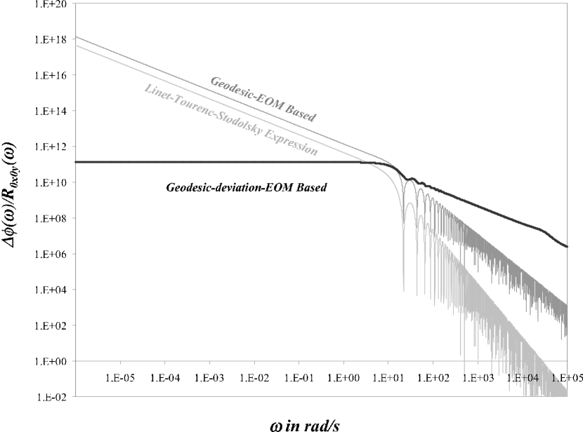
Figure 2: A plot of $\Delta\phi(\omega)/R_{0x0y}(\omega)$ versus $\omega$ for $\Delta\phi_{GD}$, $\Delta\phi_{geo}$, and $\Delta\phi_{LTS}$, for the interferometer Fig. 1 using $L_{\bot}=1.2$ m, $L_{\|}=4$ km, $T=0.58$ s, $Q=1$, $\omega_{0}=31,000$ rad/s, and used ⁶Li with $m=1\times 10^{-23}$ gm.

IV Previous Phase-shift Calculations

We now compare results of the above calculations with those done previously in the literature.

IV.1 Calculations done at the quantum-mechanical level

Calculations of the phase shift by Linet and Tourrenc Linet-Tourrenc (1976), and Stodolsky Stodolsky (1979) were both done at the quantum-mechanical level, but unlike us, they presented a completely general analysis, and did not take the nonrelativistic limit for the interfering particles they considered. Their expressions for the phase shift were thus manifestly covariant. Linet and Tourrenc did not explicitly define the coordinate system that they used, while Stodolsky only referred to the presentation by Landau and Lifschitz Landau (1962) on synchronous reference frames. It is clear that since a gravitational wave in the TT gauge has $h_{0\mu}=0$, the TT coordinates is a synchronous reference frame as well. Since both calculations were ultimately based on the action for the geodesic EOM, they were implicitly done in the TT coordinates.

Linet and Tourrenc used the WKB approximation in the quasi-classical limit, and replaced the mass-shall constraint $g^{\mu\nu}p_{\mu}p_{\nu}=-mc^{2}$ (note that the signature of their metric is different from ours) with a differential equation in the phase of the wavefunction for the test particle by making the substitution $p_{\mu}=(i/\hbar)\partial_{\mu}$. Stodolsky worked directly with the action, and used the quasi-classical approximation we followed here to calculate the phase shift. The expression for the phase shift derived by both nevertheless have the same overall form. The phase shift (given in Eq. [3.2.3] of Linet-Tourrenc (1976)) derived by Linet and Tourrenc does, however, differ from the original phase shift (given in Eq. (2.4) of Stodolsky (1979)) derived by Stodolsky by a factor of 2. Since Stodolsky uses the Linet and Tourrenc phase shift expression (the equation above Eq. (6.1) of Stodolsky (1979)) to calculate the phase shift for a model interferometer, we will do so also. In the nonrelativistic limit of the atoms that we are interested in, this phase shift reduces to

$$\Delta\phi_{LTS}=\frac{1}{2}\frac{m}{\hbar}\oint v^{i}v^{j}h_{ij}dt,$$ (31)

which is different from $\Delta\phi_{geo}$, even though both were calculated in TT coordinates.

To understand the origin of the difference between $\Delta\phi_{LTS}$ and $\Delta\phi_{geo}$, let us write $S_{geo}=S_{geo}^{kin}+S_{geo}^{pot}$, where

$$S_{geo}^{kin}=\frac{1}{2}m\int\vec{v}^{\>2}dt,\qquad S_{geo}^{pot}=\frac{1}{2}m\int v^{i}v^{j}h_{ij}dt,$$ (32)

and the superscript “kin” stands for “kinetic”, while the superscript “pot”stands for “potential”. Clearly, $\Delta\phi_{geo}=\Delta\phi^{kin}_{geo}+\Delta\phi^{pot}_{geo}$. Since $\Delta\phi_{LTS}=\Delta\phi^{pot}_{geo}$, contributions to the total phase shift $\Delta\phi^{kin}_{geo}$ from changes to the kinetic energy of the test particle as it traverses the interferometer was not taken into account in Eq. $(\ref{Stod-PS})$. This kinetic term cannot be neglected, however. The passage of the gravitational wave through the system will cause shifts in the velocity of the atom as it traverses the interferometer, and thus to its kinetic energy. In fact, by using Eqs. $(\ref{geosolutions-first})$ and $(\ref{geosolutions-second})$, it is straightforward to show that $\Delta\phi^{kin}_{geo}=-2\Delta\phi^{pot}_{geo}+B.T.$, where $B.T.$ are boundary terms for the atoms at the mirrors. These terms do not vanish, but instead contribute the $4\>\hbox{sinc}\>(\omega T/4)$ term to $F_{geo}$.

If we nonetheless use $\Delta\phi_{LTS}$ to calculate the phase shift for Fig. 1, we once again find that $\Delta\phi_{LTS}$ has the same form as Eqs. $(\ref{PhaseGeoRes})$ and $(\ref{F-GD})$,

$$\Delta\phi_{LTS}(\omega)\equiv -\frac{m}{2\hbar}L_{\|}L_{\bot}i\omega h_{\times}(\omega)e^{-i\omega T/2}F_{LTS}(\omega T),$$

$$F_{LTS}(\omega T)= -\bigg{[}\hbox{sinc}\,(\omega T/4)\bigg{]}^{2}.$$ (33)

The final result of our comparison of phase-shift calculations for the interferometer shown in Fig. 1 is given in Eq. $(\ref{F-Stod})$. While these equations, like Eq. $(\ref{PhaseGeoRes})$, are also based on the geodesic equation of motion using the TT coordinates, $F_{LTS}$ nonetheless differs from $F_{geo}$ by the term $4\>\hbox{sinc}\,(\omega T/4)$. This term comes directly from the boundary terms neglected in Eq. $(\ref{Stod-PS})$. (When expressed in terms of resonance functions, Eq. $(\ref{F-Stod})$ agrees, after the nonrelativistic limit is taken, with the phase shift calculated in Stodolsky (1979) up to overall factors.)

Taking the low-frequency limit, we find that $F_{LTS}\approx-1$. Thus, like $\Delta\phi_{geo}$, $\Delta\phi_{LTS}$ has the incorrect low-frequency limiting form. It also has a high-frequency behavior that is dramatically different from either $F_{geo}$ or $F_{GD}$, as can be seen in Fig. 2. In this limit, while $F_{geo}\sim 1/\omega T$ and $F_{GD}\sim 1$ (see appendix C), $F_{LTS}\sim 1/(\omega T)^{2}$, and dies off much more rapidly. As pointed out in nmMIGO (2003), this rapid die off is due to three effects. Firstly, the $\Delta\phi_{LTS}$ does not include the boundary terms at the mirror. These terms depend on the value of the velocity of the atom at the surface of the mirror, and the length $L_{\|}/2$, and they mitigate this rapid decrease for $\Delta\phi_{geo}$. Secondly, $\Delta\phi_{LTS}$ depends on $v^{2}$, and is constant as the atom travels through the interferometer, while $\Delta\phi_{GD}$ depends on the product $xv$, and increases linearly with the distance the atom travels from the initial beam splitter. Thirdly, since $\Delta\phi_{LTS}$ depends only on $v^{i}v^{j}h_{ij}$, discontinuous jumps in the velocity due to the hard wall mirrors were not taken into account in $\Delta\phi_{LTS}$. From appendix C, these hard-wall jumps contribute directly to the high-frequency behavior of $\Delta\phi_{GD}$.

IV.2 Calculations done at the quantum-field-theory level

IV.2.1 For Spin 0 Fields

Calculations of the phase shift at the quantum-field-therapy level were first done by Cai and Papini Papini (1989). Their starting point is the covariant version of the Ginzburg-Landau equation, but for a charged particle. This is a relativistic Klein-Gordon equation for a bosonic field $\varphi$ that interacts with itself through a $|\varphi|^{4}$ interaction (Eq. (2.1) of Papini (1989)). By turning off the $|\varphi|^{4}$ interaction, and setting the charge of the particle to zero, one recovers Linet and Tourrenc’s starting point. If one extracts the single-particle Hamiltonian from this equation, and take the correspondence principle limit of the EOM, one recovers the geodesic EOM used by Stodolsky. Thus, like Linet and Tourrenc, and Stodolsky, Cai and Papini work in TT coordinates.

By acting on $\varphi$ with a phase operator $\chi$, Cai and Papini was able to solve for a general expression for the phase shift due to gravitational effects in the weak-gravity limit through a stationary-phase type of analysis. This operator has the form [Eq. (3.1) of Papini (1989)],

$$\chi=\left\{-\frac{1}{4}\oint_{\gamma}dz^{\lambda}\left(\Gamma_{\alpha,\lambda\beta}-\Gamma_{\beta,\lambda\alpha}\right)J^{\alpha\beta}+\frac{1}{2}\oint_{\gamma}dz^{\lambda}g_{\lambda\beta}P^{\beta}\right\},$$ (34)

(using our notation) for a closed path where $J_{\alpha\beta}$ is the generator of Lorentz transformations, and $P^{\alpha}$ is the generator of translations. We have dropped the vector potential term since the atoms we consider in this paper are not charged. As they mentioned, using Stokes’ theorem the first term in $\chi$ can be written as

$$-\frac{1}{4}\int_{\cal D}R_{\mu\nu\alpha\beta}J^{\alpha\beta}d\tau^{\mu\nu},$$ (35)

in the weak-gravity limit; the integral is over the timeline surface $\cal D$ bounded by $\gamma$, and $d\tau^{\mu\nu}$ is a 2-form on $\cal D$. This expression has been explicitly verified in Chiao (2003) for the phase shift caused by Riemann curvature tensor for a stationary spacetime.

The second term agrees with Stodolsky’s expression for the phase shift. Indeed, Cai and Papini uses Eq. $(\ref{chi})$ to calculate the phase shift of a model interferometer due to the passage of a gravitational wave [Eq. (3.15) of Papini (1989)], and they found that up to terms of order $(v/c)^{2}$, the following holds:

“The $\Delta\chi_{2}$ terms in (3.15) agrees with Stodolsky’s result [11] when a misprint in the latter is corrected by inserting an overall factor $\frac{1}{2}$.” (From page 415 of Papini (1989).)

The reference [11] cited above is the work by Stodolsky cited as Stodolsky (1979) in this paper. Consequently, their expression for the phase shift, like Linet and Tourrenc’s, and Stodolsky’s, also has the incorrect low-frequency limiting form. The effects of the mirrors on the test particle’s phase was not considered by them either.

IV.2.2 For Spin 1/2 Fields

Bordé and coworkers Borde1 (1994); Borde2 (1997); Borde3 (2001) considered the use of fermionic atoms in matter-wave interferometers to measure various gravitational effects, including the detection of gravitational waves. Their starting point was the Dirac equation for a two-level, spin 1/2 atom expressed in curved spacetimes using the tetrad formalism. Similar to Cai and Papini, theirs was a Hamiltonian-based approach, and they showed that the dominant contribution by the gravitational wave to the Hamiltonian is from a term with the form $p_{i}p_{j}h^{ij}/2m$, where $m$ is the mass of the atom, and $p_{i}$ its momentum [see Eq. (10) of Borde1 (1994)]. The other terms in the Hamiltonian due to the gravitational wave are from very small spin-gravitation couplings. These terms can be neglected here since we are dealing with atoms without spin. When this is done, the Hamiltonian they calculated has the same form as Eq. $(\ref{geoham})$ for the geodesic EOM, and is manifestly different from the Hamiltonian Eq. $(\ref{GDHam})$ for the geodesic deviation EOM. Thus they, too, worked in the TT coordinates.

Although an expression for the phase shift was not calculated in Borde1 (1994), they concluded the following:

“The phase shift, that one can calculate from the first terms of Eq. (10), increases with the velocity of the atoms in contrast with what happens in the inertial field case and a gravitational wave detector using atomic interferometry should therefore use relativistic atoms. In this case, it can be shown directly from Eq. (5) that the phase shift is proportional to $h_{(\times,+)}\oint ds/\lambda$ where $\lambda$ is the atomic de Broglie wavelength, result which is similar to the optical case.” (From page 161 of Borde1 (1994).)

In a subsequent paper Borde3 (2001), Bordé gave an explicit expression for the phase shift [see Eq. (98) of Borde3 (2001)]. It has, for its spin 0 component, the same expression, $\Delta\phi_{LTS}$, for its phase shift as Stodolsky’s. Thus, like Stodolsky’s approach, any phase shift calculated using this analysis would have the incorrect low-frequency limiting form as well.

IV.2.3 More General Analysis

Finally, all of the analyses that we outlined in this paper were done in the weak-gravity limit. In Alsing (2001), a derivation of the phase shift of a quantum mechanical test particle was done without making this approximation. Their analysis was also based on the geodesic-EOM approach, and they arrived same expression for the phase shift that Stodolsky does for spin 1/2 test particle with no approximations, while it holds only the first order in $\hbar$ for spin 0 and spin 1 particles. Consequently, phase shifts calculated with their expression will also have the same incorrect low-frequency limiting form as Stodolsky’s.

V Concluding Remarks

There has been a preference among those who study matter-wave interferometry and gravitational waves to use TT coordinates to analyze the phase shift of an interferometer induced by gravitational waves instead of the proper reference frame. The expectation is that irrespective of which reference frame is used to calculate the phase shift, the final expression will be the same Thorne (1987); Unruh-Weiss . We have shown in this paper that for matter-wave interferometry this expectation is wrong. By presenting a calculation of the phase shift using the TT coordinates following the line of the analysis found in the literature Linet-Tourrenc (1976); Stodolsky (1979); Papini (1989); Borde1 (1994); Borde2 (1997); Borde3 (2001); Alsing (2001), and also a calculation of the phase shift using the proper reference frame following the analysis found in nmMIGO (2003); CrysMIGO (2003), we have shown that the expressions for the phase shift obtained using the TT-coordinates is different from that obtained using the proper reference frame. Moreover, we have shown that the commonly accepted expression for the phase shift Eq. $(\ref{Stod-PS})$—which is the end result of all previous derivations of the phase shift in the literature Linet-Tourrenc (1976); Stodolsky (1979); Papini (1989); Borde1 (1994); Borde2 (1997); Borde3 (2001); Alsing (2001)—is incomplete, and gives yet a different expression for the phase shift of Fig. 1. This happens even though derivations of this expression were all done in TT coordinates.

The focus of this paper has been on demonstrating in detail that differences exist between the various approaches to calculating the phase shift, and showing explicitly that different expressions for the phase shift are obtained. To determine which one, if any, is correct, we noted that in the limit of sufficiently low frequency gravitational waves, the correct expression for the phase shift must reduce to the well known expression for the phase shift induced by a static curvature. It must therefore be proportional to components of the Riemann curvature tensor. This static phase shift can also be calculated within Newtonian gravity, where the curvature is formed from gradients of the acceleration due to gravity $g$. The phase shift due to $g$ has been measured COW ; ChuKas , and recently has been used to measure gradients in $g$ as well PCC ; Kas ; PrivateKas . In addition, there are indications that the phase shift induced by the static Riemann curvature tensor has already been seen PrivateKas . We have explicitly shown that when the phase shift is calculated using the proper reference frame and geodesic deviation EOM, it has the expected limiting form in the low-frequency limit, and is therefore correct. The other two, both of which used the TT coordinates and the geodesic EOM, do not, and are thus incorrect.

The implications of this conclusion are immense. In nmMIGO (2003); CrysMIGO (2003), MIGO, the Matter-wave Interferometric Gravitational-wave Observatory, was proposed. The theoretical sensitivity predicted for MIGO was based on a calculation of its phase shift using the proper reference frame and the geodesic deviation EOM. The conclusion arrived at in these papers was that by using slow atoms, it would be possible to construct gravitational wave observatories that are as sensitive as LIGO or LISA (the Laser Interferometer Space Antenna), but would be orders of magnitude smaller, and have a much broader frequency response. This conclusion is diametrically opposite from the conclusions arrived previous in the literature that fast atoms—indeed, ultrarelativistic ones—should be used in the matter-wave interferometer instead Borde1 (1994).

The conclusion that relativistic atoms should be used in the detection of gravitational waves with matter-wave interferometers is the basis on which most of the atomic, molecular and optical physics community judges the suitability of using matter-wave interferometers as gravitational wave detectors. The physical origin of this conclusion by Bordé and his coworkers is the dependence of the phase shift $\Delta\phi_{LTS}$ on the square of the atom’s velocity in the geodesic-EOM-based approach; clearly, the faster the atom, the larger the phase shift will be. Even though our analysis of the phase shift was done for nonrelativistic atoms, we note that if the size of the interferometer is held constant, and only the velocity of the atom is increased, then in the high-velocity limit, $T\to 0$, and eventually $\omega T<<\pi/4$ for the frequency of gravitational waves expected from astrophysical sources. The high-velocity limit is thus equivalent to the low-frequency limit for the gravitational waves, and we have shown that the low-frequency limit of $\Delta\phi_{LTS}$ is incorrect. Thus, Bordé and coworker’s assertion about relativistic atoms being more suitable for the detection of gravitational waves is also incorrect.

All previous calculations and estimates of the phase shift in the literature also neglected the effect the mirrors of the interferometer have on the phase shift. Indeed, from appendix C we see that it is precisely because hard wall mirrors are used—along with the instantaneous impulsive force that they exert on the atoms when they reflect off—that the use of slow-velocity atoms leads to a sensitivity that increases with frequency is obtained. This dependence on frequency is the exact opposite for LIGO and LISA Thorne (1987), and is part of the reason that MIGO can be so much smaller than either one.

We have not, in this paper, presented the underlying physical reasons why the current TT coordinates approach to calculating the phase shift fails, and the proper reference frame succeeds. We shall address this issue in detail later ADS-Chiao-2004 . Here, we only note that one may try to modify the boundary conditions for the atom on the mirrors so that the phase shift calculated for Fig. 1 in TT coordinates will have the correct low-frequency limit. Doing this is especially tempting in light of the following statement by Thorne:

“However, errors are much more likely in the TT analysis than in the proper-reference-frame analysis, because our physical intuition about how experimental apparatus behaves is proper-reference-frame based rather than TT-coordinate based. As an example, we intuitively assume that if a microwave cavity is rigid, its walls will reside at fixed coordinate locations $x^{j}$. This remains true in the detector’s proper reference frame (aside from fractional changes of order $(L^{2}/\lambdabar^{2})h$, which are truly negligible if the detector is small and which the proper-reference-frame analysis ignores). But it is not true in TT coordinates; there the coordinate locations of a rigid wall are disturbed by fractional amounts of order $h$, which are crucial in analyses of microwave-cavity-based gravity wave detectors.” (From page 400 of Thorne (1987).)

We find that while it may be possible to suitably modify the boundary conditions to bring $\Delta\phi_{geo}$ in line with the low frequency limit, doing so will be ad hoc, and will not explain the underlying physical reason for the differences between $\Delta\phi_{geo}$ and $\Delta\phi_{GD}$. What is at the heart of the physics are not questions of which boundary conditions to take and how they should be modified, but rather how measurement of physical quantities are made in general relativity when the background metric varies with time.

When doing an experiment to measure some physical property of a test particle—its phase shift, say—we start by choosing an origin for our coordinate system. It is natural to choose as this origin some point on our measuring apparatus, which in our case is the initial beam splitter. In the three spatial dimensions, this origin is represented by a point on a three-dimension space; this point is what we use when measurements with a physical apparatus are actually made. If we wish to represent the origin in space and time, it would seem to be natural to represent it as an event in four-dimensional spacetime. Coordinate systems constructed by doing so are called quasi-cartesian coordinate systems by Synge. He also noted who also noted that a suitable choice of origin in spacetime for is often difficult (see section 10 of Synge (1960)), however. This is especially true in the case of gravitational waves, where the metric is nonstationary, and varies with time. In fact, by identifying the origin as an event, we have ignored the fact that our measuring apparatus is a physical object. It too must travel along a worldline in the spacetime, as will any test particle whose physical properties we are measuring. As was argued in general laboratory frame (2003), only relative motions of a test particle with respect to the apparatus can thus be measured. These arguments were based in part on the following observation by Hawking and Ellis:

“In chapter 3 we saw that if the metric was static there was a relation between the magnitude of the timelike Killing vector and the Newtonian potential. One was able to tell whether a body was in a gravitational field by whether, if released from rest, it would accelerate with respect to the static frame defined by the Killing vector. However, in general, space-time will not have any Killing vectors. Thus one will not have any special frame against which to measure acceleration; the best one can do is to take two bodies close together and measure their relative acceleration [emphasis added].” (From page 78 of Hawking (1973).)

This relative motion is not measured in the TT coordinates where the coordinates are defined relative to a fixed event, chosen as the origin, in the spacetime. The motion of the measuring apparatus through spacetime was not taking into account in the TT coordinates, so that the beam splitters and the mirrors are at fixed coordinate values. This relative motion, on the other hand, is measured in the proper reference frame where the coordinates are explicitly constructed to span the distance between the measuring apparatus, and the test particle whose properties are to be measured. The motion of the measuring apparatus has been built in from the beginning, and indeed, the positions of the beam splitters and the mirrors shift during the passage of the gravitational wave. Failing to take into account the motion of the measuring apparatus in spacetime is the underlying physical reason why the wrong expression was obtain for Fig. 1 when the TT coordinates are used.

These statements will be expanded upon, and justified in ADS-Chiao-2004 .

Appendix A The Quasi-classical Approximation and the Interferometer

In this appendix we set the framework used in our different calculations of the phase shift.

A.1 The quasi-classical approximation

Like Stodolsky Stodolsky (1979); Alsing (2001), we use the quasi-classical approximation to calculate the phase shift of an atom in a matter-wave interferometer. This approximation is the Lagrangian version of the WKB, or stationary phase approximation, in the Schrödinger representation of quantum mechanics. We assume that the density of particles through the interferometer is low enough that they do not interact with one another appreciably in the time it takes for the atom to traverse the interferometer. Within this approximation, the particles can be treated as test particles that interact only with the gravitational wave, and not with themselves. We can thus consider the phase shift of each atom individually, and use the Feynman path integral method to calculate its phase shift. However, instead of integrating over all possible paths, we make the quasi-classical approximation, and consider only the most probable path—which is also the classical path—that the test particle takes through the interferometer (see Berman (1997)). As a result,

$$\Delta\phi\approx\frac{1}{\hbar}\bigg{\{}S_{cl}[x_{A},x_{B};\gamma_{1}]-S^{cl}[x_{A},x_{B};\gamma_{2}]\bigg{\}},$$ (36)

where the superscript “cl” stands for “classical”, and $\gamma_{1}$ and $\gamma_{2}$ are the two possible paths a classical test particle can take through the interferometer that links a common point $x_{A}$ on the interferometer (the initial beam splitter, say) to a common point $x_{B}$ on the interferometer (the final beam splitter, say). Note that $S_{cl}[x_{A},x_{B};\gamma]$ are functionals of the points $x_{A}$ and $x_{B}$, along with the paths $\gamma_{1}$ and $\gamma_{2}$ connecting them.

Unlike Stodolsky (1979), as well as the calculations of the phase shift done in Linet-Tourrenc (1976); Papini (1989); Borde1 (1994); Borde2 (1997); Borde3 (2001); Alsing (2001), we will work in the nonrelativistic limit. The reason for doing so is two fold. First, the proper reference frame, as well as the general laboratory frame and all the other reference frames based on the worldline of an observer, are constructed for nonrelativistic test particles. Second, as is well known, the phase shift of a matter-wave interferometer is proportional to the mass of the particle. This argues for the use of atoms in matter-wave interferometers to detect gravitational waves, as was proposed in nmMIGO (2003); CrysMIGO (2003), and in any conceivable matter-wave interferometer, these atoms will be moving nonrelativistically.

A.2 The interferometer

The configuration of the interferometer that we use in our calculations is shown in Fig. 1. Details of this interferometer can be found in nmMIGO (2003). For our purposes, it is sufficient to note that the interfering test particle in the interferometer is an atom with mass $m$. A beam of these atoms is emitted from an atomic source with velocity $v_{s}$, and is beam-split into different diffraction orders using a diffraction grating with periodicity $a$ (see Pritchard (1991); Borde4 (1991); Zeilinger (1999)). Only the $n=+1$ and $n=-1$ diffraction orders are used in the interferometer.

There are two possible paths, denoted as $n=+1$ and $n=-1$ in Fig. 1, that any individual atom can follow through the interferometer; it is not possible to tell a priori which of the two paths an atom will take. If the atom is diffracted into the $n=+1$ diffraction order, then immediately after the beam splitter it will have a velocity of $+v_{\bot}=2\pi\hbar/ma$ perpendicular to the longitudinal axis of the interferometer. Similarly, if an atom is diffracted into the $n=-1$ diffraction order, it will have a velocity of $-v_{\bot}$ (see Fig. 1). Since the diffraction grating does not impart energy to the atom, for both diffraction orders $v_{\|}=(v_{s}^{2}-v_{\bot}^{2})^{1/2}$ is the velocity of the atom parallel to the axis of the interferometer immediately after it leaves the beam splitter.

In nmMIGO (2003); CrysMIGO (2003) the use of hard-wall, specular reflection mirrors was considered for the matter-interferometer. Mirrors of this type have been made from silicon wafers Holst (1999), and for near normal and near glancing angles, the reflection from these mirrors is close to 100%. These are not the mirrors that are currently used in matter-wave interferometry, however. Mirrors based on diffraction gratings, standing waves of light, or stimulated Raman pulses are used instead Pritchard (1991); Borde4 (1991); Zeilinger (1999); ChuKas ; Kas . We will nevertheless consider only the case of hard-wall mirrors in this paper, because of their simplicity. In the absence of gravitational waves, the effect of hard-wall mirrors, if they do not move, on the velocity of the atoms through the interferometer is

$$v_{x}(out)=v_{x}(in),\qquad v_{y}(out)=-v_{y}(in),$$ (37)

where $\vec{v}(in)$ and $\vec{v}(out)$ are, respectively, the velocity of the atom immediately before it is reflected off the mirror, and immediately afterwards.

Appendix B The TT gauge and the General Laboratory Frame

In this appendix we will show how the TT gauge can be taken in the general laboratory frame in a treatment that follows general laboratory frame (2003).

Like the proper reference frame, the general laboratory frame is an orthonormal coordinate system fixed on the worldline of an observer. In our case it is fixed on the worldline of the initial beam splitter in Fig. 1. We choose a local tetrad $e^{A}_{\>\>\>\>\mu}$ fixed on the observer’s worldline. Thus, $e^{A}_{\>\>\>\>\mu}e_{A\nu}=g_{\mu\nu}$, while $e_{A}^{\>\>\>\>\mu}e_{B\nu}=\eta_{AB}$. In a slight break in the notation followed elsewhere in this paper, which follows the notational convention established in Thorne (1987), we use in this appendix the convention taken in general laboratory frame (2003). Thus, we use as the tetrad indices capital Latin letters, which run from 0 to 3. Lower-case Latin letters are used as the spatial tetrad indices, and they run from 1 to 3. As usual, Greek letters are used for the spacetime indices of a general coordinate $x^{\mu}$.

Consider a the motion of a test particle $\cal P$ close to the observer $\cal O$ and her worldline. Let $X^{A}(\tau)$ be the position of $\mathcal{P}$ at any proper time $\tau$ in the observer’s frame. $X^{A}(x):x^{\mu}\to X^{A}$ can also be considered as a coordinate transformation from the general coordinates $x^{\mu}$ to the tetrad frame at any time $\tau$. Thus in a small neighborhood $\mathcal{U}_{\mathcal{O}}$ of $\mathcal{O}$,

$$\eta_{AB}\>dX^{A}dX^{B}=\eta_{AB}\frac{\partial X^{A}}{\partial x^{\mu}}\bigg{|}_{\mathcal{U}_{\mathcal{O}}}\frac{\partial X^{B}}{\partial x^{\nu}}\bigg{|}_{\mathcal{U}_{\mathcal{O}}}dx^{\mu}dx^{\nu},$$ (38)

so that

$$\frac{\partial X^{A}}{\partial x^{\mu}}\bigg{|}_{\mathcal{U}_{\mathcal{O}}}=e^{A}_{\>\>\>\>\mu},\qquad\hbox{or}\qquad\frac{\partial x^{\mu}}{\partial X^{A}}\bigg{|}_{\mathcal{U}_{\mathcal{O}}}=e_{A}^{\>\>\>\>\mu}.$$ (39)

Integrating Eq. $(\ref{8})$, we find for the spatial coordinates

$$X_{a}(\tau)=\int_{\mathit{\gamma}_{\chi}^{\tau}(0)}^{\mathit{\gamma}_{\chi}^{\tau}(s_{1})}e_{a\mu}(\tau,s)\chi^{\mu}(\tau,s)ds\equiv\int_{\mathit{\gamma}_{\chi}^{\tau}(s)}\bm{e}_{a}.$$ (40)

where $\bm{e}_{A}=e_{A\mu}dx^{\mu}$ is a 1-form, and $\gamma_{\chi}$ is a space-like geodesic linking $\cal O$ to $\cal P$ at a given proper time $\tau$ of the observer. Next, after taking appropriate account of causality, the time component is

$$X_{0}(t)=-\left(\tau-\tau^{\prime}\right)+\int_{\mathit{\gamma}_{\pi}(\sigma)}\bm{e}_{0}.$$ (41)

where $\gamma_{\pi}$ is a null-vector linking $\cal O$ at time $\tau^{\prime}$ with $\cal P$ at time $\tau$; the difference $\tau-\tau^{\prime}$ is the transit time of a light pulse emitted by $\cal O$, and scattered by $\cal P$.

In the case of linearized gravity, $g_{\mu\nu}=\eta_{\mu\nu}+h_{\mu\nu}$. It is straightforward to see that in terms of tetrads

$$e_{A}^{\>\>\>\>\mu}=\left(\delta^{\mu}_{\nu}-\frac{1}{2}h^{\mu}_{\nu}\right)\delta_{A}^{\nu},\quad\hbox{and }\qquad e^{A}_{\>\>\>\>\mu}=\left(\delta_{\mu}^{\nu}+\frac{1}{2}h_{\mu}^{\nu}\right)\delta^{A}_{\nu}.$$ (42)

This choice is not unique. If one does a local Lorentz transformation $L_{A}^{\>\>\>\>\tilde{A}}$ on $e_{A}^{\>\>\>\>\mu}$, then $\eta_{AB}=L_{A}^{\>\>\>\>\tilde{A}}L_{B\tilde{A}}$ while $e_{A}^{\>\>\>\>\mu}=L_{A}^{\>\>\>\>\tilde{A}}e_{\tilde{A}}^{\>\>\>\>\mu}$. This leaves $g_{\mu\nu}=e_{A\mu}\>\>e^{A}_{\>\>\>\>\nu}=e_{\tilde{A}\mu}\>\>e^{\tilde{A}}_{\>\>\>\>\nu}$ invariant.

The usual derivation of the TT gauge makes use of a remnant of general coordinate transformation invariance still left in the linearized-gravity limit of general relativity. If $x_{\mu}=\tilde{x}_{\mu}+\xi_{\mu}$ where $\xi_{\mu}$ is a ‘small’, arbitrary vector, then $h_{\mu\nu}$ transforms to

$$\tilde{h}_{\mu\nu}=h_{\mu\nu}+\partial_{\mu}\xi_{\nu}+\partial_{\nu}\xi_{\mu}.$$ (43)

One can choose $\xi_{\mu}$ such that

$$\eta^{\mu\nu}h_{\mu\nu}=0,\qquad\partial^{\mu}h_{\mu\nu}=0,\qquad h_{0\mu}=0,$$ (44)

can be chosen for GWs in Minkowski space. Doing so defines a specific coordinate system, which is called the TT coordinates in Thorne (1987).

The TT gauge can also be implemented in the general laboratory frame as well. In terms of a tetrad frame, the linearized coordinate transformation Eq. $(\ref{trans})$ induces a Lorentz transformation on the tetrads such that $e^{\tilde{A}}_{\>\>\>\>\mu}=L^{\tilde{A}}_{\>\>\>\>A}e^{B}_{\>\>\>\>\mu}$, where

$$L^{\tilde{A}}_{\>\>\>\>A}=\delta^{\tilde{A}}_{\>\>\>\>A}+\frac{1}{2}\left(\partial^{\tilde{A}}\xi_{A}+\partial_{A}\xi^{\tilde{A}}\right),$$ (45)

and $\partial_{A}=e_{A}^{\mu}\partial_{\mu}$. Like the TT coordinates, the TT gauge can also be realized, but now through the appropriate Lorentz transformation. From Eq. $(\ref{8})$, this in turn means we can choose the TT gauge in the construction of the general laboratory frame as well.

Appendix C The High-frequency Limit

In this appendix we consider the high-frequency limit of $\Delta\phi_{GD}$.

Because of its dependence on three timescales, the analysis of the high-frequency limit of $\Delta\phi_{GD}$ is more involved than that for the low frequency limit. There are two cases to consider. The simplest case is when the transit time of the atom through the interferometer is very long in comparison with the period of the gravitational wave, so that $T>>2\pi/\omega$, but $\omega<<\omega_{0}$ still. To the atom, the mirrors still do not move in response to the gravitational wave, but the atom will experience many oscillations of the gravitational wave as it traverses the interferometer. In this limit the phase of the atom oscillates so fast that we would naively expect the phase shift to average to zero. It does not do so, however. We instead find that $F_{GD}\sim 1$.

That $\Delta\phi_{GD}$ does not vanish in the limit of high-frequency gravitational waves is due to action of the mirrors on the atoms as they traverse through the interferometer. When the atoms reflect of the mirrors, they impart a impulsive force on the atoms that is effectively instantaneous . The effect of this force is readily apparent from the discontinuity in $v_{y}$ across the mirror in Eqs. $(\ref{bc})$ and $(\ref{pertGeobc})$. Note in particular that the force is proportional to perturbed velocity $v_{1y}(t_{r}+T^{-1}/2)$ of the atom caused by the gravitational wave, and is different depending on which path the atom travels through the interferometer, as can be seen from the force lines in Fig. 1. It is because of this net instantaneous force that $\Delta\phi_{GD}$ does not average to zero in the high-frequency limit.

When, $\omega>>\omega_{0}$ as well, the mirrors themselves oscillate rapidly as the atom traverses the interferometer. This rapid motion of the mirror is not correlated with the motion of the atoms through the interferometer, however. When the atom reaches the mirror, roughly half the time it will be moving in the same direction as the mirror, which would, from Eq. $(\ref{GeoDevBC})$, tend to decelerate the atom. The other half of the time it will be moving in the opposite direction as the mirror, and would tend to accelerate the atom. Not surprising, in this limit the resonance function decreases by a half, and $F_{GD}\approx 1/2$.

In this high-frequency limit $\Delta\phi_{GD}$ is not proportional to $R_{0x0y}$. There is no reason to expect it to be, as there was in the low-frequency limit, however. Because the mirrors exert a net force—which itself is the result of the passage of the gravitational wave through the system—on the atom as it passes through the interferometer, $\Delta\phi_{GD}\sim\Gamma^{x}_{0y}$.