Reinstating Schwarzschild’s original manifold and its singularity

Abstract. A review of results about this paradigmatic solution to the field equations of Einstein’s theory of general relativity is proposed. Firstly, an introductory note of historical character explains the difference between the original Schwarzschild’s solution and the “Schwarzschild solution” of all the books and the research papers, that is due essentially to Hilbert, as well as the origin of the misnomer.

The viability of Hilbert’s solution as a model for the spherically symmetric field of a “Massenpunkt” is then scrutinised. It is proved that Hilbert’s solution contains two main defects. In a fundamental paper written in 1950, J.L. Synge set two postulates that the geodesic paths of a given metric must satisfy in order to comply with our basic ideas on time, namely the postulate of order and the non-circuital postulate. It is shown that neither Hilbert’s solution, nor the equivalent metrics that can be obtained from the latter with a coordinate tranformation that is regular and one-to-one everywhere except on the Schwarzschild surface can obey both Synge’s postulates. Therefore they do not possess a consistent arrow of time, and the only way for obviating this defect is through a change of topology. The true raison d’être of the Kruskal maximal extension with its odd doubling and bifurcate horizon stays just in its capability to produce the needed change of topology, that can be demonstrated through a constructive cut-and-past procedure applied to two Hilbert space-times.

The second main defect of Hilbert’s space-time is constituted by the existence of an invariant, local, intrinsic quantity with a simple operational interpretation that diverges when it is calculated at a position closer and closer to Schwarzschild’s surface, i.e. at an internal position in Hilbert’s metric. The diverging quantity is the norm of the four-acceleration of a test particle whose worldline is the unique orbit of absolute rest defined, through a given event, by the unique timelike, hypersurface orthogonal Killing vector. It is an intrinsic quantity, whose local definition only requires the knowledge of the metric and of its derivatives at a given event, just like it happens with the polynomial invariants built with the Riemann tensor and with its covariant derivatives. The regularity of the latter invariants at a given event has been considered by many a relativist like a “rule of thumb” proof of regularity for the manifold at that event, in the persistent lack of a satisfactory definition of local singularity in general relativity.

The divergence of the above mentioned norm of the four-acceleration, i.e. of the first curvature of the worldline, is a geometric fact. It can be proved however with an exact argument, relying on a two-body solution found by Bach, that a physical quantity, the norm of the force per unit mass exerted on a test particle in order to keep it on the orbit of absolute rest, is equal to the norm of the four-acceleration, hence it diverges too on approaching Schwarzschild’s surface.

We claim that the rôle and interpretation of topological differences between partly isometrical manifolds as well as that of the singularities is not really settled, in particular that the Schwarzschild solution and its topological relatives are in more ways singular than the invariants of the Riemann tensor indicate.

Due to these facts we assert that the topology chosen by Schwarzschild should be taken as a serious alternative to the commonly used Hilbert or Kruskal topologies.

1. Introduction: Schwarzschild’s original solution and the “Schwarzschild solution”

The content of this review would be hardly understandable without a proviso of historical character: Schwarzschild’s original solution, as undisputably testified by Schwarzschild’s “Massenpunkt” paper [1], describes a manifold that is different from the one defined by the solution that goes under the name of Schwarzschild in practically all the books and the research articles written by the relativists in nearly nine decades. That solution must be instead credited to Hilbert [2]. The readers should not be induced by this assertion into believing that it is our intention to deprive Schwarzschild of the merit of his discovery, and to attribute it to the later work by Hilbert. It is not so: an accurate reading of Schwarzschild’s paper and of the momentous Communication by Hilbert [3] shows in fact that, while Schwarzschild’s derivation of the original solution is mathematically flawless, Hilbert’s rederivation contains an error. Due to this overlooked flaw, Hilbert’s manifold happened to include Schwarzschild’s manifold, but by chance it resulted not to be in one-to-one correspondence with it. This fact was deemed rather irrelevant by Hilbert, but soon developed into a conundrum that puzzled theoreticians like Marcel Brillouin [4], and had to become of crucial importance more than forty years later. In fact the birth of the black hole idea, as noted for the first time by Abrams [2], can be considered just a legacy of Hilbert’s magnanimity.

Schwarzschild’s paper, in which it is reported the first derivation of the field of a “Massenpunkt” according to general relativity, is an impressive example of mathematical precision and clearness of exposition. For the sake of definiteness in the subsequent discussion, an English translation [5] of that paper is provided in Appendix A.

On reading Schwarzschild’s paper, one immediately notes [6] that the equations he set out to solve in the special case of a static, spherically symmetric field are not the final equations of general relativity [7, 8] found by Einstein and by Hilbert, specialised for the case of vacuum. In fact, equations (A.4) and (A.5) are the vacuum equations for the next-to-last version of the theory [9] that Einstein communicated to the Prussian Academy of Sciences on November 11th, 1915. These equations yield, in vacuo, the same solutions as the equations of the final theory of November 25th, but their covariance is limited to the unimodular transformations.

Due to this fact, it was highly inconvenient for Schwarzschild to avail, as symmetry adapted coordinates, of the usual spherical polar coordinates $r$, $\vartheta$, $\varphi$, $t$, since the functional determinant of the transformation from Cartesian to such polar coordinates is $r^{2}\sin\vartheta\neq 1$; he had rather adopting polar coordinates with the determinant 1, defined by equation (A.7). Using these coordinates $x_{i}$, the square of the symmetry adapted line element ${\rm d}s^{2}$ is written by Schwarzschild, in equation (A.9), by means of $f_{1}$, $f_{2}=f_{3}$, $f_{4}$, i.e. three independent functions of the radial coordinate $x_{1}$. These functions must fulfill the conditions enumerated just after that equation: Minkowskian behaviour at the spatial infinity, field equations, inclusive of the equation of the determinant, and continuity everywhere, except at the origin.

When these conditions are obeyed, with the exception of the last one, the three independent functions $f_{1}$, $f_{2}$, $f_{4}$ were found by Schwarzschild to be given by equations (A.12), (A.10) and (A.11) respectively. They contain two independent integration constants, $\alpha$ and $\rho$. By appealing to Newton, Schwarzschild obtained that $\alpha$ had, in his units, just twice the value of the active gravitational mass. The remaining constant $\rho$ was instead determined by Schwarzschild by imposing his last condition, namely the continuity of the components of the metric. The function $f_{1}$ is in fact discontinuous when $3x_{1}=\alpha^{3}-\rho$. For a given $\alpha$, the choice of a given value for $\rho$ changes the position of the discontinuity in the interval of definition $[0,+\infty[$ of the radial coordinate $x_{1}$. It can also bring the discontinuity outside it. Therefore the choice of $\rho$ fixes the very choice of the manifold that describes the field of a “Massenpunkt”. The requirement of continuity everywhere, except at the origin, led Schwarzschild to set $\rho=\alpha^{3}$, i.e. to locate at the inner border of the manifold the discontinuity that would have been named, after him, “the singularity at the Schwarzschild radius”.

Let us compare now Schwarzschild’s determination of the manifold representing the static, spherically symmetric gravitational field with the later derivation done by Hilbert [3]. For ease of comparison, an English translation for the relevant part of the second of Hilbert’s Communications entitled “Die Grundlagen der Physik” is reproduced in Appendix B. Hilbert could avail of the generally covariant, final version of the theory, that he himself had contributed to establish with his first Communication [8] bearing the same title. Hence he could adopt the usual spherical polar coordinates and write the line element for a spherically symmetric, static $g_{\mu\nu}$ field like in expression (B.42). Thereby the line element is made to depend on three arbitrary functions $F(r)$, $G(r)$, $H(r)$, where $r$ is a radial coordinate, whose range, in keeping with its definition in term of the Cartesian coordinates $w_{i}$, is given by $0\leq r<+\infty$. But, while Schwarzschild’s choice of a line element depending on three arbitrary functions was not redundant, since he had to fulfill both the field equations and the condition of the determinant, Hilbert’s line element, after satisfying the field equations, would still contain one arbitrary function. Therefore Hilbert chose to fix one of the three functions $F(r)$, $G(r)$, $H(r)$ by defining a new radial coordinate $r^{\ast}$ such that $r^{\ast}=\sqrt{G(r)}$. Then, of course, he was entitled to drop the asterisk and write the line element with two unknown functions $M(r)$ and $W(r)$, like in expression (B.43), that has become the canonical starting point for all the textbook derivations of the “Schwarzschild solution”. As correctly remarked by Abrams [2], what neither Hilbert nor, in his footsteps, the subsequent generations of relativists were entitled to do was assuming without justification that the physical range of the new radial coordinate is still $0\leq r<+\infty$. In fact, this is equivalent to inadvertently make the restrictive choice $G(0)=0$ in expression (B.42).

The new radial coordinate allowed Hilbert to avail of a straightforward method of solution, based on the bright, although mathematically unwarranted shortcut: writing the symmetry restricted action for the problem under study and applying a symmetry restricted variational principle to it; the correctess of the resulting solution is thereby not ensured, and must be checked afterwards. In this way Hilbert eventually found the line element of equation (B.45), that, at variance with Schwarzschild’s result, depends on just one integration constant, $\alpha$, again interpreted as twice the active gravitational mass. The discontinuity in the coefficient of ${\rm d}r^{2}$, that is the counterpart of the discontinuity exhibited by the function $f_{1}(x_{1})$ in Schwarzschild’s equation (A.12), in Hilbert’s solution is fixed at $r=\alpha$, because in Hilbert’s calculation there is no free integration constant, like the $\rho$ of Schwarzschild, to move it around. This is the consequence of the unduly restrictive choice $G(0)=0$, i.e. of Hilbert’s lapse, and by no means a necessary consequence of Einstein’s equations. Einstein’s equations do not fix the topology, and additional reasoning is necessary to do so.

Nevertheless, Schwarzschild’s original solution and manifold, that were the result of a mathematically correct procedure and of the pondered choice of the integration constant $\rho$, went soon forgotten. Hilbert’s solution and manifold, that were on the contrary the consequence of the inadvertent fixing of an integration constant, were instead handed down to the posterity as the unique “Schwarzschild solution”. A contribution to the rooting of the misnomer undoubtedly came from Schwarzschild’s premature death. But the main responsibility for it should be attributed to Hilbert himself, given his exceptional, well deserved standing in the community of the mathematicians, astronomers and physicists of his time, and of ours.

In fact, while dismissing, in a short footnote, Schwarzschild’s procedure of removing the discontinuity to the origin as “not advisable”, Hilbert attributed to Schwarzschild the finding of his own solution (B.45), hence of the manifold inadvertently chosen by himself, the one for which $0\leq r<+\infty$, with its two singularities located at $r=0$ and at $r=\alpha$ in what the relativists would have called “Schwarzschild coordinates”.

However such features, that would have so much bothered generations of scholars, were only of very marginal interest for the great Hilbert. As it appears from the enthusiastic, last words of his Communication [8] of 1915, he harbored the firm conviction that, by starting from just two very simple axioms, thanks to the powerful instruments constituted by the calculus of variations and by the theory of invariants, he had succeded in embodying both Einstein’s new conceptions about gravitation and Mie’s new ideas about electrodynamics [10, 11] into a mathematical structure of lasting value. In Hilbert expectations, only the full theory would have been capable to provide an immediate representation of reality, at any scale, through everywhere regular solutions. Hence, one should not worry if the first, very partial soundings into the exact mathematical content of the theory, done by neglecting the fundamental ingredient of the electromagnetic field, exhibited, together with the confirmation of Einstein’s achievement [12] about the perihelion of Mercury, a singular behaviour of difficult interpretation.

2. The wrong arrow of time of Hilbert’s manifold is at the origin of the Kruskal extension

It is not here the place to recall in detail how it happened that the relativists gradually abandoned the attitude to look in general relativity for the simile of the notion of singularity that had been so useful in the mathematical physics of the past. That ideal conception is well reflected in the very notion of regularity of the interval and of the metric that Hilbert provided just at the end of his derivation of the “Schwarzschild solution”. According to Hilbert’s definition, the singularities exhibited by the components of the metric both at $r=0$ and at $r=\alpha=2m$ were true singularities of the field $g_{\mu\nu}$, because they could not be erased by invertible, one-to-one transformations of coordinates. The notions of regularity and of singularity set by Hilbert went unchallenged, with some notable exceptions, till the half of the past century, when they found also a sharpened definition [13] in the book by Lichnerowicz. It should be remarked here that Hilbert’s definitions of regularity and of allowable coordinate transformations not only represented the extension to the new theory of time-honoured conceptions of mathematical physics, but were in keeping with Einstein’s own ideas on the meaning of general covariance [14]. According to Einstein, it was in fact necessary to divest space and time coordinates of the last residuum of physical objectivity, but for one aspect. For him, all the assertions of physics could be reduced in the last instance to assertions about events, physically embodied by spacetime coincidences between particles. The introduction of spacetime coordinates is a convenient instrument for reckoning such coincidences. But for the coordinates to absolve their residual physical function, it is necessary that the transformations of coordinates do preserve the individuality of the single event. There is therefore one sound physical reason why the allowed transformations must be invertible and one-to-one, as required by Hilbert.

Einstein’s conception of the “Bezugmolluske” and the connected definition of regularity by Hilbert would have resisted the lapse of the decades, if the manifolds of general relativity had been truly Riemannian, rather than pseudo-Riemannian, like they happen to be, and if the singular surface at $r=\alpha$ in the Hilbert solution had not had null lines as generators. This is why the doubt first arose about the true nature of the “singularity at the Schwarzschild radius”. Along each one of the generators it is ${\rm d}s^{2}=0$. Does it mean that we have to do with a light path, or does it mean that this generator is not a worldline, but just one and the same event, misrepresented in a coordinate system in which an inadequate choice of the coordinate chart has created, together with the singularity of the metric, the illusion of the presence of a light line? If so, why not try to find, through some disallowed coordinate transformation, appropriately singular at $r=\alpha$, a new coordinate chart in which the light line, for all the finite values of the Hilbert coordinate time $t$, would become associated with just one value of the new coordinate time, and the metric would become regular at $r=\alpha$?

After preliminary attempts that succeeded in the second task, but not in the first one [15, 16, 17], both tasks were eventually accomplished together by Synge [18] in a ground-breaking, now nearly forgotten paper. In its footsteps came the results by Fronsdal, Kruskal and Szekeres [19, 20, 21] about the so-called maximal extension of the Schwarzschild manifold. Of course, in order to accomplish both tasks, Synge had to infringe the rules about the admissible transformations set by Einstein and Hilbert. Synge’s ideas about the definition of singularities in general relativity are worth mentioning, because they were very clear, and pessimistic. With some reason, one may add, because the situation, as we shall see in the sequel, has not greatly improved since the time Synge’s paper [18] appeared in print. Synge wrote:

Obviously, before we talk of singularities at all, we should define them. Adequate definitions should be invariant, but there are difficulties here which may not appear on the surface. It is true that some of these difficulties are overcome by a limitation to regular transformations, but it is precisely the non-regular transformations which are interesting. Thus we must satisfy ourselves for the present with definitions dependent on the coordinate system employed.

And then he provided his coordinate-dependent definition:

Definition. A form $g_{mn}{\rm d}x^{m}{\rm d}x^{n}$ has a component singularity at a point $x^{r}=a^{r}$ which lies in a region $R$ of the representative space $V_{4}$ or on the boundary of $R$, if one or more of the components $g_{mn}$ has no unique finite limit, independent of path, as we approach $a^{r}$ through $R$; and it has a determinantal singularity if the determinant $g$ of $g_{mn}$ has not a unique finite non-zero limit as we approach $a^{r}$ through $R$.

In keeping with this definition, one may assert that Synge and his followers had succeeded, by an appropriately singular transformation, in removing the singularity that the metric components exhibit at $r=\alpha$. They had also succeeded, by the same singular transformation, in reducing the points with finite $t$ coordinate on each one of the generators of the singular surface $r=\alpha=2m$ to have one and the same coordinate time in the new chart. As a consequence of this second achievement, it became possible to draw and explore mathematically how the timelike and the null geodesics prevailing in the regions of Hilbert’s manifold with $r<\alpha$ and with $r>\alpha$ respectively happen to connect smoothly at $r=\alpha$. Such a connection could not be properly explored in the original coordinates adopted by Hilbert, because in these coordinates the connection of the geodesics occurs when $t\rightarrow\pm\infty$, as it is hinted by Figure (1a).

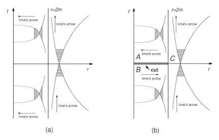
Figure 1. (a): Representation of Hilbert’s manifold in the $r$, $t$ plane. Light cones are drawn both in the inner region and in the outer region. Time arrows are schematically drawn in keeping with the non-circuital postulate. The postulate of order is thereby violated. (b) A cut is made in Hilbert’s manifold. The topologically different manifold obtained in this way allows for a consistent drawing of the time arrow.

One can now notice that Synge and his followers, with their singular coordinate transformations, had reached a third achievement too. This further result is usually given scarce or no relevance at all in the literature, although e.g. Rindler did not forget to make a fugitive mention of it in his book [22]. In order to appreciate its full value, one has rather resorting once more to Synge, were a detailed discussion of the issue of the time arrow can be found [18]. According to Synge, a manifold meant to be a model of physical reality must fulfill two postulates. One of them is the postulate of order, according to which the parameter of proper time along a timelike geodesic must always either decrease or increase; the sense along which it is assumed to increase defines the sense of the travel from past to future, namely the time arrow. Since the geodesic equation is quadratic in the line element, fixing the time arrow of the individual geodesic is a matter of choice. The second postulate deals with our ideas of causation, and establishes a relation between the time arrows of neighbouring geodesics. Synge calls it the non circuital postulate. It asserts that there cannot exist in space-time a closed loop of time-like geodesics around which we may travel always following the sense of the time-arrow.

Synge shows in detail [18] that the time arrow can be drawn in keeping with the aforementioned postulates in the manifold that he obtained from the Hilbert manifold with his singular coordinate transformation; the same property obviously holds in the Kruskal-Szekeres manifold too. Does it hold also in the Hilbert manifold? A glance to Figure (1a) is sufficient to gather that this is not the case. The arrow of time can be drawn correctly in the submanifold with $r>\alpha$, i.e. in Schwarzschild’s original manifold, and separately in the inner submanifold with $r<\alpha$. A consistent drawing of the arrow of time, in keeping with both postulates, is however impossible in Hilbert’s manifold as a whole. This is an intrinsic flaw of the latter manifold; it has nothing to do either with the fact that in Hilbert’s chart the metric is not defined at $r=\alpha$, or with the fact that the timelike geodesics appear to cross the Schwarzschild surface at the coordinate time $t=\pm\infty$; it is a flaw that cannot be remedied by any coordinate transformation, however singular at $r=\alpha$, but one-to-one elsewhere.

The only known ways to overcome this flaw are either by getting rid of the inner region, thereby reinstating the original manifold [1], deliberately chosen by Schwarzschild as a model for the gravitational field of a material particle, or by completely renouncing the one-to-one injunction on the coordinate transformations set, on physical grounds, by Einstein and by Hilbert.

The second alternative is the one chosen by Synge and his followers: in fact, not only Schwarzschild’s original manifold, but also Kruskal’s manifold avoids the flaw of the arrow of time present in Hilbert’s manifold. Moreover, it appears to preserve its inner region. However, it does so by a coordinate transformation that duplicates the original manifold and alters its topology, in a way that is best explained, rather than by looking at the equations for the transformation, by a straighforward cut-and-paste procedure applied to two Hilbert manifolds.

This cut-and-past procedure can be realised in infinite ways, all entailing an alteration of topology. One of them is accounted for in the sequence drawn in Figures (1b), (2a) and (2b).

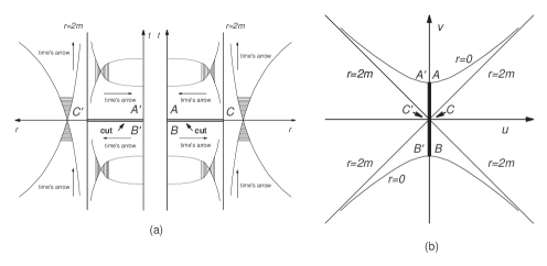
Figure 2. (a) two manifolds, equal to the cut Hilbert manifold of Figure (1b) are juxtaposed for suturing; (b) sewing together the edges $ACB$ and $A^{\prime}C^{\prime}B^{\prime}$ yields Kruskal’s manifold.

In Figure (1b) the inner region of the Hilbert manifold of Figure (1a) is cut along the line $AC$. The resulting manifold is topologically inequivalent to the Hilbert manifold. The topological alteration already allows to draw the arrows of time in keeping with Synge’s postulates but, due to the existence of the border $ACB$, the new manifold is evidently unphysical. However, if one takes two manifolds identical to the one of Figure (1b), juxtaposes them as it is shown in Figure (2a), and eventually sews together the borders $ACB$ and $A^{\prime}C^{\prime}B^{\prime}$ like in Figure (2b), one obtains Kruskal’s manifold, and ascertains that the arrows of time inherited from the two component manifolds with the cut still obey both Synge’s postulates.

Therefore, rather than discarding it, like one does with the Schwarzschild manifold, one can save the inner region of Hilbert’s manifold at the cost of changing the topology of the latter with a cut, that is then remedied by the doubling intrinsic to the Kruskal-Szekeres manifold. The mathematical beauty of the latter is beyond question. Its physical usefulness much less so, if, after having examined at length the properties of the Kruskal metric, textbooks usually end the discussion by asserting that this indissoluble union of a white and a black hole hardly has anything to do with some entity really present in Nature. It is usually added that black holes should be meant as the final result of the process of collapse, in which only part of the Kruskal manifold would be involved. It is however evident that entering such arguments means abandoning the discussion of actually existing, well scrutinised vacuum solutions to the field equations of general relativity, and venturing, despite the huge amount of work done on the subject, in uncharted waters.

Anyway, when confronted with the Kruskal manifold, with its odd doubling and its bifurcate horizon, we eventually gather how serious is the flaw of the arrow of time in Hilbert’s manifold, if one could conceive resorting to such extreme surgical means in order to remove just that flaw.

3. An invariant, local, intrinsic quantity that diverges at the Schwarzschild surface

We have called Synge’s ideas about the issue of the definition of a singularity in general relativity clear and pessimistic. His coordinate-dependent definition is in fact a clear mirror of the difficulties that he met with. Of course he would have had rather availing of an invariant definition of singularity, because in such a way the problem of defining what coordinate transformations were allowable would have become much less challenging. In fact, a scalar would maintain its value, no matter whether the transformations of coordinates should be limited to the ones allowed for by Einstein and Hilbert, or whether Synge’s “interesting” transformations, namely nonregular ones, thereby capable of canceling the singular behaviour of the metric at $r=\alpha$ in Hilbert’s solution, could be allowed too. However, no general enough, physically satisfactory, invariant definition of singularity was available to him. A posteriori one must recognise that Synge’s pessimism was justified, because for decades the problem has been ingeniously tackled by several authors (see for instance [23, 24, 25, 26] [27, 28, 29, 30]) who proposed several solutions but, by the admission [29] of some of them, it is also possible that “there may not exist any useful, generally applicable notion of the singular boundary of a space-time”.

Synge’s coordinate-dependent definition, on the other side, cannot be a satisfactory answer if the nonregular transformations are decreed legitimate, for then the locus $r=\alpha$ is either singular or regular according to whether it is looked at in the Hilbert chart rather than in the Eddington-Finkelstein [15, 16] or Kruskal charts respectively.

In the persistent lack of a physically satisfactory, general, invariant definition of singularity, and due also to the growing awareness that Synge’s [31] identification “gravitational field = curvature of space-time” had to be substituted for Einstein’s old idea that in general relativity the gravitational field was represented by the Christoffel symbols, the scalar invariants built with the Riemann tensor, whose singularity is certainly sufficient for proving the singularity of a manifold, began to be used, for lack of a better alternative, as invariant, local, intrinsic indicators of its regularity too.

In the case of the Kruskal manifold, the latter scalar invariants provided the same verdicts about singularity and ad ignorantiam regularity as Synge’s coordinate dependent definitions applied in the Kruskal chart: the singularity at $r=\alpha$ is fictitious, due to the choice of the coordinates, while the singularity at $r=0$ is a true one, intrinsic to the manifold.

There is however one argument that suggests that such invariants might not be as trustful indicators of regularity as they are generally believed to be. Metrics endowed with spherical symmetry are indeed very special items. When availing of a given metric, endowed with a high degree of symmetry, as a model of physical reality, one would like not to incur the following, perplexing situation: as soon as a certain symmetry of the metric is lifted, one of its essential properties, as measured by some scalar quantity, changes abruptly, no matter how small it is the deformation that destroys the original symmetry.

Let us consider what is generally called a static spacetime, namely a pseudoRiemannian manifold that admits a timelike Killing vector that is hypersurface orthogonal; this Killing vector $\xi_{i}$ fulfills the equations:

(3.1) $$\xi_{i}\xi^{i}>0,\ \ \xi_{i;k}+\xi_{k;i}=0,\ \ \xi_{[i}\xi_{k,l]}=0.$$

In symmetry adapted coordinates $x^{0}$, $x^{1}$, $x^{2}$, $x^{3}$, the line element of a static spacetime reads

(3.2) $${\rm d}s^{2}=\sum_{\alpha,\beta=1}^{3}g_{\alpha\beta}(x^{1},x^{2},x^{3}){\rm d}x^{\alpha}{\rm d}x^{\beta}+V^{2}({\rm d}x^{0})^{2},\ \ V=V(x^{1},x^{2},x^{3}).$$

Let us assume the line element to enjoy the following properties:

• the metric is a vacuum solution of Einstein’s field equations, regular and Minkowskian at spatial infinity;

• the equipotential surfaces $V=C=$ const.$>0$, $x^{0}=$ const. are regular, simply connected, closed 2-surfaces;

• the intrinsic geometry of the 2-surfaces $V=C,x^{0}=$ const., tends to that of a closed regular 2-surface of finite area in the limit $C\rightarrow 0$;

• the Kretschmann scalar $R_{iklm}R^{iklm}$ is everywhere finite.

Then a surprising theorem, found [32] by Israel, asserts that the only spacetime that fulfills the hypotheses enumerated above is Schwarzschild’s original manifold [1]. Of course, Israel’s theorem does not say which of the hypotheses happens to fail when the static spacetime is not Schwarzschild’s original manifold; this detail can be learned on a case by case basis. One interesting example is provided by the so called gamma metric.

The latter is one of the axially symmetric, static vacuum solutions [33] calculated in 1922 by Bach, who availed of the general method of solution [34, 35] found by Weyl and by Levi-Civita. Despite the nonlinear structure of Einstein’s equations, Weyl succeeded in reducing the axially symmetric, static problem to quadratures through the introduction of his “canonical cylindrical coordinates”. Let $x^{0}=t$ be the time coordinate, while $x^{1}=z$, $x^{2}=r$ are the coordinates in a meridian half-plane, and $x^{3}=\varphi$ is the azimuth of such a half-plane; the adoption of Weyl’s canonical coordinates allows writing the line element of a static, axially symmetric field in vacuo as:

(3.3) $${\rm d}s^{2}=e^{2\psi}dt^{2}-{\rm d}\sigma^{2},\;e^{2\psi}{\rm d}\sigma^{2}=r^{2}{\rm d}\varphi^{2}+e^{2\gamma}({\rm d}r^{2}+{\rm d}z^{2});$$

the two functions $\psi$ and $\gamma$ depend only on $z$ and $r$. Remarkably enough, in order to provide a solution to Einstein’s equations, $\psi$ must fulfill the “Newtonian potential” equation

(3.4) $$\Delta\psi=\frac{1}{r}\left\{\frac{\partial(r\psi_{z})}{\partial z}+\frac{\partial(r\psi_{r})}{\partial r}\right\}=0,$$

where $\psi_{z}$, $\psi_{r}$ are the derivatives of $\psi$ with respect to $z$ and to $r$ respectively, while $\gamma$ is obtained by solving the system

(3.5) $$\gamma_{z}=2r\psi_{z}\psi_{r},\;\gamma_{r}=r(\psi^{2}_{r}-\psi^{2}_{z});$$

due to equation (3.4)

(3.6) $${\rm d}\gamma=2r\psi_{z}\psi_{r}{\rm d}z+r(\psi^{2}_{r}-\psi^{2}_{z}){\rm d}r$$

happens to be an exact differential.

The particular Bach’s metric we are interested in is defined by choosing for $\psi$ the potential that, in Weyl’s “Bildraum”, is produced by a thin massive rod of constant linear density $\sigma=k/2$ lying on the symmetry axis, say, between $z=z_{2}=-l$ and $z=z_{1}=l$, that acts as source for the “Newtonian potential” of equation (3.4). One then finds:

(3.7) $$\psi=\frac{k}{2}\ln\frac{r_{1}+r_{2}-2l}{r_{1}+r_{2}+2l},$$

where

(3.8) $$r_{i}=[r^{2}+(z-z_{i})^{2}]^{1/2},\;i=1,2.$$

By integrating equations (3.5) and by adjusting an integration constant so that $\gamma$ vanish at the spatial infinity one obtains:

(3.9) $$\gamma=\frac{k^{2}}{2}\ln\frac{(r_{1}+r_{2})^{2}-4l^{2}}{4r_{1}r_{2}}.$$

The resulting metric is asymptotically flat at spatial infinity and its components are everywhere regular, with the exception of the segment of the symmetry axis for which $z_{2}\leq z\leq z_{1}$, for any choice of the parameters $l$ and $k$, assumed here to be positive.

It may be convenient [36] to express the line element in spheroidal coordinates by performing, in the meridian half-plane, the coordinate transformation [37]:

(3.10) $$\varrho=\frac{1}{2}(r_{1}+r_{2}+2l),\;\cos\vartheta=\frac{r_{2}-r_{1}}{2l}.$$

Then the interval takes the form

(3.11) $$ds^{2}=\left(1-\frac{2l}{\varrho}\right)^{k}{\rm d}t^{2}$$

$$-\left(1-\frac{2l}{\varrho}\right)^{-k}\left[\left(\frac{\Delta}{\Sigma}\right)^{k^{2}-1}{\rm d}\varrho^{2}+\frac{\Delta^{k^{2}}}{\Sigma^{k^{2}-1}}{\rm d}\vartheta^{2}+\Delta\sin^{2}\vartheta{\rm d}\varphi^{2}\right],$$

where

(3.12) $$\Delta=\varrho^{2}-2l\varrho,\;\Sigma=\varrho^{2}-2l\varrho+l^{2}\sin^{2}\vartheta.$$

Therefore, provided that $k\neq 0$, the component $g_{00}=V^{2}$ of this static metric exhibits closed, simply connected 2-surfaces on which $V=C$, and $C\rightarrow 0$ when $\varrho\rightarrow 2l$, in partial fulfillment of the hypotheses set by Israel. We note that when $k=1$ the metric reduces to Schwarzschild’s spherically symmetric one. It does so in the strict sense: it is in one-to-one correspondence with Schwarzschild’s original solution [1], not with Hilbert’s manifold [3]. The latter would be retrieved from (3.11) with $k=1$ if the radial coordinate $\varrho$ were allowed the range $0\leq\varrho<\infty$ while, due to (3.10), the allowed values of $\varrho$ are presently in the range $2l\leq\varrho<\infty$. Therefore, when $k=1$ the manifold fulfills all the hypotheses set by Israel.

Let us now explore the behaviour, as a function of $k$, of the Kretschmann scalar $K\equiv R_{iklm}R^{iklm}$ of the gamma metric. The calculation and the study of this scalar has been done long ago [37] by Cooperstock and Junevicus, and was recently repeated by Virbhadra. We quote here his result [38], expressed with spheroidal coordinates:

(3.13) $$K=\frac{16l^{2}k^{2}N}{\varrho^{2(k^{2}+k+1)}(\varrho-2l)^{2(k^{2}-k+1)}\Sigma^{3-2k^{2}}},$$

with

(3.14) $$N =l^{2}\sin^{2}\theta\left[3lk(k^{2}+1)(l-\varrho)+k^{2}(4l^{2}-6l\varrho+3\varrho^{2})+l^{2}(k^{4}+1)\right]$$

$$+3\varrho[(k+1)l-\varrho]^{2}(\varrho-2l).$$

We do not need a minute analysis of the function $K(\rho,\vartheta,k)$ for noting that, when $\rho\rightarrow 2l$, the Kretschmann scalar is a discontinuous parameter in the set of the gamma metrics. It is sufficient to examine its behaviour in the neighbourhood of $k=1$, for arbitrarily small axially symmetric deviations from spherical symmetry. By studying the zeroes of both the numerator and the denominator of (3.13) one is then confronted with the following situation. For all the values of $\vartheta$, the denominator vanishes when $\rho\rightarrow 2l$, while the values of $\varrho$ at which the zeroes of the numerator occur depend on both $k$ and $\vartheta$. Hence in the neighbourhood of $k=1$ the Kretschmann scalar always diverges [37] for $\rho\rightarrow 2l$, provided that $k\neq 1$. When $k=1$, and the metric reduces to Schwarzschild’s one, both the numerator and the denominator tend to zero as $\rho\rightarrow 2l$ for all $\vartheta$, and they do so in such a way that the limit value of the Kretschmann scalar happens to be finite at the “Schwarzschild radius”. Therefore, in the particular case of the gamma metric, Israel’s theorem leads to this occurrence: the slightest deviation from the spherical symmetry of Schwarzschild’s manifold destroys the regularity of the Kretschmann scalar for $\rho\rightarrow 2l$. This is a troublesome result, because the latter regularity is a necessary condition for the extension of the Schwarzschild manifold to the inner region. The above mentioned slightest deviation from the spherical symmetry renders the procedure of extension impossible.

One may conclude, like Israel did [39] in a worried letter to “Nature”, that “models with exact spherical symmetry possess idiosyncrasies which render them dangerous, and perhaps misleading, as a basis for induction”. One may instead wonder whether, at least in this case of static manifolds, one had rather imputing the idiosyncrasies not to the spherical symmetry, but to the chosen indicator of singularity, and whether a more reliable indicator might exist. At variance with the polynomial scalars built with the Riemann tensor, in the case of the gamma metric this indicator, hopefully endowed with physical meaning, should not exhibit a discontinuous behavior, as a function of $k$, when $\rho\rightarrow 2l$. In the search of such an alternative indicator, we can look into the history of general relativity, and draw inspiration from the ideas about the entity representing the gravitational field that prevailed before Synge set his identification [31] of the gravitational field with the curvature of spacetime. For Synge that assertion was not an abstract, a priori statement; it was instead rooted in the sort of physical reasoning that had led him, already in 1937, to reject [40] Whittaker’s identification of the gravitational pull [41].

In compliance with Einstein’s principle of equivalence [14], Whittaker had assumed that the gravito-inertial force exerted on a pole test particle of unit mass, whose worldline was a congruence with unit tangent vector $u^{i}(x^{k})$, was defined by minus the first curvature vector $a^{i}$ of the congruence:

(3.15) $$a^{i}=\frac{{\rm d}u^{i}}{{\rm d}s}+\Gamma^{i}_{kl}u^{k}u^{l},$$

namely, by minus the four-acceleration of the test particle. If one thinks that in general relativity the gravito-inertial pull should balance the nongravitational forces, (3.15) can be read like the extension of Newton’s second law to the new theory. This extension does not need to be postulated: it can be derived from the conservation identities of the theory, and it indeed asserts that the force per unit mass $a^{i}$ exerted by, say, the electromagnetic field on the pole test particle is balanced by minus the gravito-inertial pull per unit mass expressed by the right-hand side of (3.15).

Synge criticised Whittaker’s definition of the gravito-inertial pull on the ground that in Einstein’s theory only relative kinematic measurements involving nearby particles are permitted in general, hence one must renounce the unattainable goal of determining absolutely the force acted by the gravitational field on any particle, and must be content with a differential law that only allows for the comparison of the gravitational pull acting at adjacent events. Let us consider then two pole test particles, both executing geodesic motion, and imagine that their world-lines $L$, $M$ be very close to each other. If $\eta^{i}$ is the infinitesimal displacement vector drawn perpendicular to $L$ from a point $A$ on $L$ to a point $B$ on $M$, the acceleration of $B$ relative to $A$ is defined by the infinitesimal vector

(3.16) $$f^{i}=\frac{{\rm D}^{2}\eta^{i}}{{\rm d}s^{2}},$$

where ${\rm D}/{\rm d}s$ indicates absolute differentiation and ${\rm d}s$ is the infinitesimal arc length of the geodesic $L$ measured at $A$. But Synge himself [43] had proved that

(3.17) $$\frac{{\rm D}^{2}\eta^{i}}{{\rm d}s^{2}}+R^{i}_{~{}jkl}u^{j}\eta^{k}u^{l}=0,$$

where $R^{i}_{~{}jkl}$ is the Riemann tensor and $u^{i}$ is the four-velocity of the particle at $A$. By appealing to Newton, Synge postulated that the excess of the gravitational force at the event $B$ over the gravitational force at the event $A$ is defined (for unit test masses) to be the acceleration (3.16) of $B$ relative to $A$. Hence he found [40] that the excess of the gravitational pull is given by

(3.18) $$f^{i}=-R^{i}_{~{}jkl}u^{j}\eta^{k}u^{l}.$$

Therefore, leaving behind Einstein’s principle of equivalence, through the equation of geodesic deviation the identification between gravitational field and curvature entered the theory of general relativity; subsequently the polynomial invariants built with the Riemann tensor became indicators of the singularity and ad ignorantiam regularity of the gravitational field.

One may observe, however, that just in the case of the static manifolds Synge’s objection, that in Einstein’s theory only relative kinematic measurements are permitted, hence “one must be content with a differential law that only allows for the comparison of the gravitational pull acting at adjacent events”, is not true.

To understand why, it is necessary a sharpening of the definition of static manifold, that is generally overlooked. We have reported earlier that definition, both in the coordinate form and in the intrinsic one, provided by equations (3.1), according to which a manifold is static if it is endowed with a timelike, hypersurface orthogonal Killing vector. Such a definition, however, applies also to the Minkowski spacetime.

The attribution of the adjective “static” to the Minkowski spacetime does not seem however to be an appropriate one. In fact, the notion of staticity is undisputably associated with the notion of rest. How is it possible to call “static” the metric of the theory of special relativity, a theory that denies intrinsic meaning to the very notion of rest? How is it possible that the Minkowski metric remain static, as it does according to our definition, after we have subjected it to an arbitrary Lorentz transformation, i.e. a transformation that entails relative, uniform motion? Let us start from the Minkowski metric, given by $g_{ik}={\rm diag}(-1,-1,-1,1)$ with respect to the Galilean coordinates $x$, $y$, $z$, $t$, and perform the coordinate transformation

(3.19) $$x=X\cosh{T},\ y=Y,\ z=Z,\ t=X\sinh{T}$$

to new coordinates $X$, $Y$, $Z$, $T$. We get the particular Rindler metric [44], whose interval reads

(3.20) $${\rm d}s^{2}=-{\rm d}X^{2}-{\rm d}Y^{2}-{\rm d}Z^{2}+X^{2}{\rm d}T^{2}.$$

How is it possible that this metric turn out to be in static form too, despite the fact that the transformation (3.19) entails uniformly accelerated motion? The definition of static manifold needs to be completed by further specifying that the timelike, hypersurface orthogonal Killing vector must be uniquely defined by equations (3.1) at each event. This is the case, for instance, with such solutions of general relativity as just Schwarzschild’s original solution and the gamma metric, provided that the curvature is nonvanishing. In these manifolds of general relativity the congruences built with the unique timelike, hypersurface orthogonal Killing vector field define wordlines of absolute rest. They are intrinsic to the manifold since, at variance with the worldlines of observers arbitrarily drawn on a manifold, they are defined by the metric alone through equations (3.1). In this case it is by no means true that only relative kinematic measurements are allowed, because a single such worldline can be recognised in an absolute way, from the local knowledge of the metric and of its derivatives. From here it follows that the first curvature (3.15) of the worldlines of absolute rest is a local and intrinsic property of a truly static manifold. There is no valid objection to Whittaker’s definition of the gravitational pull in this case: the norm $a=(-a_{i}a^{i})^{1/2}$ in this case is an invariant, local, intrinsic quantity, defined only by the metric, just like the polynomial invariants built with the Riemann tensor happen to be. In the case of the gamma metric, defined with the spheroidal coordinates (3.10) by equations (3.11) and (3.12), the squared norm of the four-acceleration of a test particle on a worldline of absolute rest reads [45]

(3.21) $$a^{2}=\frac{16k^{2}l^{2}}{[4(\varrho-l)^{2}-4l^{2}\cos^{2}\vartheta]^{1-k^{2}}(2\varrho-4l)^{1-k+k^{2}}(2\varrho)^{1+k+k^{2}}},$$

Therefore, for any value of $k<2$ and for all $\vartheta$ the norm $a$ happens to grow without limit as $\varrho\rightarrow 2l$. At variance with what occurs with the Kretschmann scalar, for $\varrho\rightarrow 2l$, $a$ does not exhibit any discontinuous behaviour when crossing the value $k=1$, for which the gamma metric specialises into the Schwarzschild metric, and the norm reduces to

(3.22) $$a=\left[\frac{l^{2}}{\varrho^{3}(\varrho-2l)}\right]^{1/2}.$$

The invariant, local, intrinsic quantity $a$, if used as indicator of singularity of a static manifold, does not suffer from the “idiosyncrasies” exhibited by the Kretschmann scalar $K$ of equation (3.13): $a$ uniformly diverges when $\varrho\rightarrow 2l$, thereby signalling the presence of an invariant, local, intrinsic singularity just on the inner border of Schwarzschild’s original manifold, hence of an inadmissible singularity in the interior of Hilbert’s manifold.

4. The singularity at the Schwarzschild surface is both intrinsic and physical

Like Synge’s definition (3.18) of the relative gravitational pull, Whittaker’s definition of the gravitational force felt by a test body of unit mass kept at rest in a static field is connected to the geometric definition of the corresponding four-acceleration (3.15) by way of hypothesis. It is true that the hypothesis is supported by the derivation from the Einstein-Maxwell equations done by Papapetrou and Urich [42]. However, given the crucial rôle that Whittaker’s definition has in determining the intrinsic singular character of Schwarzschild’s surface, it seems worth calculating this force directly from some actually existing exact solution of Einstein’s equations. In this way one may hope to ascertain whether the divergence of an invariant, local, intrinsic geometric entity is accompanied by the divergence of a physical quantity. In this section the norm of the four-force exerted on a test body in Schwarzschild’s field is obtained [46] by starting, in the footsteps of Weyl [47],[33], from a particular two-body Weyl-Levi Civita solution of Einstein’s equations, calculated in 1922 by R. Bach [33].

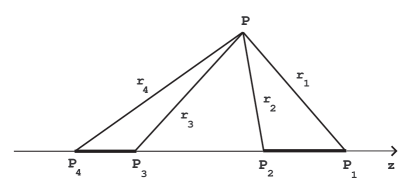
Figure 3. Representation in the canonical $z$, $r$ half-plane of the mass sources for Bach’s two-body solution. $r_{4}$, $r_{3}$ and $r_{2}$, $r_{1}$ are the “distances”, calculated in the Euclidean way, of a point $P$ from the end points of the two segments endowed with mass. $\overline{P_{4}P_{3}}=2l^{\prime}$, $\overline{P_{3}P_{2}}=2d$, $\overline{P_{2}P_{1}}=2l$, again in coordinate lengths.

By availing of Weyl’s canonical cylindrical coordinates, this static, axially symmetric two-body solution is obtained if one assumes, like Bach did, that the “Newtonian potential” $\psi$ entering the line element (3.3) is generated, in the canonical “Bildraum”, by matter that is present with constant linear mass density $\sigma=1/2$ on two segments of the symmetry axis, like the segments $P_{4}P_{3}$ and $P_{2}P_{1}$ of Figure 3. We know already from (3.7) that the particular choice

(4.1) $$\psi=\frac{1}{2}\ln\frac{r_{1}+r_{2}-2l}{r_{1}+r_{2}+2l}+\frac{1}{2}\ln\frac{r_{3}+r_{4}-2l^{\prime}}{r_{3}+r_{4}+2l^{\prime}},$$

will produce a vacuum solution to Einstein’s field equations that reduces to Schwarzschild’s original solution if one sets either $l=0$ or $l^{\prime}=0$. Of course, due to the nonlinearity of (3.5), one cannot expect that $\gamma$ will contain only the sum of the contributions

(4.2) $$\gamma_{11}=\frac{1}{2}\ln\frac{(r_{1}+r_{2})^{2}-4l^{2}}{4r_{1}r_{2}},\;\gamma_{22}=\frac{1}{2}\ln\frac{(r_{3}+r_{4})^{2}-4{l^{\prime}}^{2}}{4r_{3}r_{4}},$$

corresponding to the individual terms of the potential (4.1); a further term is present, that Bach called $\gamma_{12}$, and reads

(4.3) $$\gamma_{12}=\ln\frac{lr_{4}-(l^{\prime}+d)r_{1}-(l+l^{\prime}+d)r_{2}}{lr_{3}-dr_{1}-(l+d)r_{2}}+c,$$

where $c$ is a constant. Since $\gamma$ must vanish at the spatial infinity, it must be $c=\ln[d/(l+l^{\prime})]$. With this choice of the constant one eventually finds [33] that the line element of the two-body solution is defined by the functions

$$e^{2\psi}=\frac{r_{1}+r_{2}-2l}{r_{1}+r_{2}+2l}\cdot\frac{r_{3}+r_{4}-2l^{\prime}}{r_{3}+r_{4}+2l^{\prime}},$$

$$e^{2\gamma}=\frac{(r_{1}+r_{2})^{2}-4l^{2}}{4r_{1}r_{2}}\cdot\frac{(r_{3}+r_{4})^{2}-4{l^{\prime}}^{2}}{4r_{3}r_{4}}$$

(4.4) $$\cdot\left(\frac{d(l^{\prime}+d)r_{1}+d(l+l^{\prime}+d)r_{2}-ldr_{4}}{d(l^{\prime}+d)r_{1}+(l+d)(l^{\prime}+d)r_{2}-l(l^{\prime}+d)r_{3}}\right)^{2}.$$

With these definitions for $\psi$ and $\gamma$ the line element (3.3) behaves properly at the spatial infinity and is regular everywhere, except for the two segments $P_{4}P_{3}$, $P_{2}P_{1}$ of the symmetry axis, where the sources of $\psi$ are located, and also for the segment $P_{3}P_{2}$, because there $\gamma$ does not vanish as required, but takes the constant value

(4.5) $$\Gamma=\ln{\frac{d(l+l^{\prime}+d)}{(l+d)(l^{\prime}+d)}},$$

thus giving rise to the well known conical singularity.

Due to this lack of elementary flatness occurring on the segment $P_{3}P_{2}$, the solution is not a true two-body solution; nevertheless Weyl showed [33] that a regular solution could be obtained from it, provided that nonvanishing energy tensor density $\mathbf{T}^{k}_{i}$ be allowed for in the space between the two bodies. In this way an axial force $F$ is introduced, with the evident function of keeping the two bodies at rest despite their mutual gravitational attraction. By providing a measure for $F$, Weyl provided a measure of the gravitational pull. Let us recall here Weyl’s analysis [47, 33] of the axially symmetric, static two-body problem.

In writing Einstein’s field equations, we adopt henceforth Weyl’s convention for the energy tensor:

(4.6) $$R_{ik}-\frac{1}{2}g_{ik}R=-T_{ik}.$$

Einstein’s equations teach that, when the line element has the expression (3.3), $\mathbf{T}^{k}_{i}$ shall have the form

(4.7) $$\left(\begin{array}[]{llll}\mathbf{T}^{0}_{0}&0&0&0\\ \\ 0&\mathbf{T}^{1}_{1}&\mathbf{T}^{1}_{2}&0\\ \\ 0&\mathbf{T}^{2}_{1}&\mathbf{T}^{2}_{2}&0\\ \\ 0&0&0&\mathbf{T}^{3}_{3}\end{array}\right)$$

where

(4.8) $$\mathbf{T}^{1}_{1}+\mathbf{T}^{2}_{2}=0.$$

By introducing the notation

(4.9) $$\mathbf{T}^{3}_{3}=r\varrho^{\prime},\;\mathbf{T}^{0}_{0}=r(\varrho+\varrho^{\prime}),$$

Einstein’s equations can be written as:

(4.10) $$\Delta\psi=\frac{1}{2}\varrho,\;\frac{\partial^{2}\gamma}{\partial z^{2}}+\frac{\partial^{2}\gamma}{\partial r^{2}}+\left\{\left(\frac{\partial\psi}{\partial z}\right)^{2}+\left(\frac{\partial\psi}{\partial r}\right)^{2}\right\}=-\varrho^{\prime};$$

(4.11) $$\mathbf{T}^{1}_{1}=-\mathbf{T}^{2}_{2}=\gamma_{r}-r(\psi^{2}_{r}-\psi^{2}_{z}),\;-\mathbf{T}^{2}_{1}=-\mathbf{T}^{1}_{2}=\gamma_{z}-2r\psi_{r}\psi_{z}.$$

Weyl shows that $\varrho$ must be interpreted as mass density in the canonical “Bildraum”. To this end he considers the mass density distribution sketched in Figure 4, where $\varrho$ is assumed to be nonvanishing only in the shaded regions labeled $1$ and $2$ respectively.

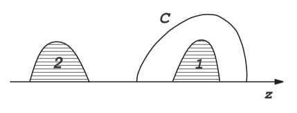
Figure 4. Representation in the canonical $z$, $r$ half-plane of extended mass sources of a two-body solution.

According to (4.1), the potential $\psi$ corresponding to this mass distribution can be uniquely split in two terms $\psi_{1}$ and $\psi_{2}$, such that $\psi_{1}$ is a potential function that vanishes at infinity and is everywhere regular outside the region $1$, while $\psi_{2}$ behaves in the same way outside the region $2$. The asymptotic forms of $\psi_{1}$ and $\psi_{2}$ are such that

(4.12) $$e^{2\psi_{1}}=1-\frac{m_{1}}{R}+\cdot\cdot\cdot,\;e^{2\psi_{2}}=1-\frac{m_{2}}{R}+\cdot\cdot\cdot$$

where the mass coefficients $m_{1}$ and $m_{2}$ are given by the integral $\int{\varrho{\rm d}V}=2\pi\int{\varrho r{\rm d}r{\rm d}z}$, performed in the canonical space and extended to the appropriate shaded region. Outside the shaded regions one has $\varrho=0$, but there shall be some region between the bodies, let us call it $L^{\prime}$, where $\varrho=0$ but $\mathbf{T}^{k}_{i}\neq 0$, since in a static solution of general relativity the gravitational pull shall be counteracted in some way. Weyl’s procedure for determining $\mathbf{T}^{k}_{i}$ in $L^{\prime}$ is the following. Suppose that $\mathbf{T}^{k}_{i}$ vanishes outside a simply connected region $L$ that includes both material bodies. Since $\psi$ is known there, we can avail of (3.6), together with the injunction that $\gamma$ vanish at infinity, to determine $\gamma$ uniquely outside $L$. Within $L^{\prime}$ we can choose $\gamma$ arbitrarily, provided that we ensure the regular connection with the vacuum region and the regular behaviour on the axis, i.e. $\gamma$ vanishing there like $r^{2}$. Since $\psi$ is known in $L^{\prime}$ and $\gamma$ has been chosen as just shown, we can use equations (4.10) and (4.11) to determine $\mathbf{T}^{k}_{i}$ there.

If the material bodies include each one a segment of the axis, just as it occurs in Fig. 4, the force $F$ directed along the $z$ axis, with which the stresses in $L^{\prime}$ contrast the gravitational pull can be written as

(4.13) $$F=2\pi\int_{C}(\mathbf{T}^{2}_{1}{\rm d}z-\mathbf{T}^{1}_{1}{\rm d}r);$$

the integration path is along a curve $C$, like the one drawn in Fig. 4, that separates the two bodies in the meridian half-plane; the value of the integral does not depend on the precise position of $C$ because, as one gathers from the definitions (4.10), (4.11):

(4.14) $$\mathbf{T}^{1}_{1,1}+\mathbf{T}^{2}_{1,2}=0$$

in the region $L^{\prime}$. Since the region of the meridian half-plane where $\varrho=0$ is simply connected, by starting from $\psi$ and from the vacuum equation (3.6), now rewritten as:

(4.15) $${\rm d}\gamma^{*}=2r\psi_{z}\psi_{r}{\rm d}z+r(\psi^{2}_{r}-\psi^{2}_{z}){\rm d}r$$

one can uniquely define there the function $\gamma^{*}$ that vanishes at the spatial infinity. In all the parts of the $z$ axis where $\varrho=0$ it must be $\gamma^{*}_{z}=0$, $\gamma^{*}_{r}=0$, hence $\gamma^{*}=$const., $\gamma^{*}_{r}=0$. In particular, in the parts of the axis that go to infinity one shall have $\gamma^{*}=0$; let us call $\Gamma^{*}$ the constant value assumed instead by $\gamma^{*}$ on the segment of the axis lying between the two bodies. The definitions (4.11) can now be rewritten as:

(4.16) $$\mathbf{T}^{1}_{1}=-\mathbf{T}^{2}_{2}=\gamma_{r}-\gamma^{*}_{r},\;-\mathbf{T}^{2}_{1}=-\mathbf{T}^{1}_{2}=\gamma_{z}-\gamma^{*}_{z},$$

and the integral of (4.13) becomes

(4.17) $$\int_{C}(\mathbf{T}^{2}_{1}{\rm d}z-\mathbf{T}^{1}_{1}{\rm d}r)=\int_{C}{(\gamma^{*}_{z}-\gamma_{z}){\rm d}z+(\gamma^{*}_{r}-\gamma_{r}){\rm d}r}=\int_{C}{\rm d}(\gamma^{*}-\gamma).$$

Since $\gamma$ vanishes on the parts of the $z$ axis where $\varrho=0$, the force $F$ that holds the bodies at rest despite the gravitational pull shall be

(4.18) $$F=-2\pi\Gamma^{*}$$

with Weyl’s definition (4.6) of the energy tensor. When the mass density $\varrho$ has in the canonical space the particular distribution considered by Bach and drawn in Fig. 3, $\Gamma^{*}$ is equal to $\Gamma$ as defined by (4.5). The measure of the gravitational pull with which the two “material bodies” of this particular solution attract each other therefore turns out to be

(4.19) $$F=2\pi\ln{\frac{(d+l)(d+l^{\prime})}{d(d+l+l^{\prime})}}$$

in Weyl’s units. This expression agrees with the Newtonian value when $l$ and $l^{\prime}$ are small when compared to $d$, as expected.

Despite its mathematical beauty, Weyl’s definition of the gravitational pull for an axially symmetric, static two-body solution appears associated without remedy to the adoption of the canonical coordinate system. It is however possible to obtain through Weyl’s definition of $F$, given by (4.13), a “quasi” four-vector $f_{i}$. In fact that expression can be rewritten as

(4.20) $$F=\int_{\Sigma}\mathbf{T}^{l}_{1}{\rm d}f^{*}_{0l}\equiv\frac{1}{2}\int_{\Sigma}T^{l}_{1}\epsilon_{0lmn}{\rm d}f^{mn},$$

where $\epsilon_{klmn}$ is Levi-Civita’s totally antisymmetric tensor and ${\rm d}f^{mn}$ is the element of the two-surface $\Sigma$ generated by the curve $C$ through rotation around the symmetry axis. Since the metric that we are considering is static in the strict sense it is possible to define a unique timelike, hypersurface orthogonal Killing vector $\xi^{k}_{(t)}$ that correspond, in Weyl’s canonical coordinates, to a unit coordinate time translation. Therefore (4.20) can be rewritten as

(4.21) $$F=\frac{1}{2}\int_{\Sigma}\xi^{k}_{(t)}T^{l}_{1}\epsilon_{klmn}{\rm d}f^{mn}$$

by still using the canonical coordinates. Now the integrand is written as the first component of the infinitesimal covariant four-vector

(4.22) $$\xi^{k}_{(t)}T^{l}_{i}\epsilon_{klmn}{\rm d}f^{mn},$$

but of course in general the expression

(4.23) $$f_{i}=\frac{1}{2}\int_{\Sigma}\xi^{k}_{(t)}T^{l}_{i}\epsilon_{klmn}{\rm d}f^{mn}$$

will not be a four-vector, because the integration over $\Sigma$ spoils the covariance. When evaluated in canonical coordinates, the nonvanishing components of $f_{i}$ are $f_{1}=F$ and

(4.24) $$f_{2}=2\pi\int_{C}(\mathbf{T}^{2}_{2}{\rm d}z-\mathbf{T}^{2}_{1}{\rm d}r)=2\pi\int_{C}{(\gamma^{*}_{r}-\gamma_{r}){\rm d}z-(\gamma^{*}_{z}-\gamma_{z}){\rm d}r},$$

that however must vanish too, if $f_{i}$ has to become a four-vector defined on the symmetry axis. But, as one sees from Weyl’s analysis, we are at freedom to choose $\mathbf{T}^{k}_{i}$ in $L^{\prime}$ as nonvanishing only in a tube with a very small, yet finite coordinate radius, that encloses in its interior the segment of the symmetry axis lying between the bodies; moreover, we can freely set $\gamma_{z}=\gamma^{*}_{z}$ within the tube. Under these conditions the second term of the integral (4.24) just vanishes, while the first one shall be very small, since the regularity of the surface $\Sigma$ requires that the curve $C$ approach the symmetry axis at a right angle in canonical coordinates. By properly choosing $\mathbf{T}^{k}_{i}$ we thus succeed in providing through equation (4.23) a quasi four-vector $f_{i}$ whose components, written in Weyl’s canonical coordinates, reduce in approximation to $(F,0,0,0)$.

Having defined, with the above caveats, the quasi four-vector $f_{i}$ along the segment of the symmetry axis between the two bodies, we can use its “quasi” norm to provide a measure of the force that opposes the gravitational pull. In the case of Bach’s two-body solution, whose line element is defined in canonical coordinates by (3.3) and (4.4), that quasi norm reads

(4.25) $$f\equiv(-f^{i}f_{i})^{1/2}=2\pi\ln\frac{(d+l)(d+l^{\prime})}{d(d+l+l^{\prime})}\cdot\left[\frac{r_{1}-2l}{r_{1}}\cdot\frac{r_{4}-2l^{\prime}}{r_{4}}\right]^{1/2}$$

when measured in Weyl’s units at a point of the symmetry axis for which $z_{3}<z<z_{2}$. At variance with the behaviour of $F$, the quasi norm $f$ depends on $z$, due to the term of (4.25) enclosed within the square brackets, that comes from $e^{2\psi}$. Let us evaluate this quasi norm divided by $l^{\prime}$ when $l^{\prime}\rightarrow 0$, namely, the coefficient of the linear term in the McLaurin series expansion of $f$ with respect to $l^{\prime}$. Since $\Gamma^{*}$, now defined by the right-hand side of (4.5), tends to zero when $l^{\prime}\rightarrow 0$, while performing this limit one can also send to zero the radius of the very narrow tube considered in the previous section. Therefore $f_{i}$ can become a true four-vector and $f$ can become a true norm in the above mentioned limit. With this proviso one finds the invariant, exact result

(4.26) $$\lim_{l^{\prime}\rightarrow 0}\left[\frac{f}{l^{\prime}}\right]=\left[\frac{\partial f}{\partial l^{\prime}}\right]_{l^{\prime}=0}=\frac{2\pi l}{d(d+l)}\left(\frac{r_{1}-2l}{r_{1}}\right)^{1/2}.$$

When $l^{\prime}\rightarrow 0$ the line element of Bach’s solution with two bodies tends to the line element defined by (3.3) and (3.7) when $k=1$, that is in one-to-one correspondence with the line element of Schwarzschild’s original solution [1]. Therefore the scalar quantity $[\partial f/\partial l^{\prime}]_{l^{\prime}=0}$ evaluated at $P_{3}$ shall be the norm of the force per unit mass exerted by Schwarzschild’s gravitational field on a test particle kept at rest at $P_{3}$. Its value is obtained by substituting $2d+2l$ for $r_{1}$ in (4.26). One finds

(4.27) $$\left(\lim_{l^{\prime}\rightarrow 0}\left[\frac{f}{l^{\prime}}\right]\right)_{z=z_{3}}=\frac{8\pi l}{(2d+2l)^{3/2}(2d)^{1/2}}.$$

If one solves Schwarzschild’s problem in spherical polar coordinates $r$, $\vartheta$, $\varphi$, $t$ with three unknown functions $\lambda(r)$, $\mu(r)$, $\nu(r)$, i.e. without fixing the radial coordinate, like Combridge and Janne did long ago [48],[49], one ends up writing de Sitter’s line element [50]

(4.28) $${\rm d}s^{2}=-\exp{\lambda}{\rm d}r^{2}-\exp{\mu}[r^{2}({\rm d}\vartheta^{2}+\sin^{2}{\vartheta}{\rm d}\varphi^{2})]+\exp{\nu}{\rm d}t^{2}$$

in terms of one unknown function $h(r)$. In fact $\lambda$, $\mu$, $\nu$ are defined through this arbitrary function $h(r)$ and through its derivative ${h^{\prime}}(r)$ as follows:

(4.29) $$\exp{\lambda}=\frac{{h^{\prime}}^{2}}{1-2m/h},$$

(4.30) $$\exp{\mu}=\frac{h^{2}}{r^{2}},$$

(4.31) $$\exp{\nu}=1-2m/h.$$

Here $m$ is the mass constant; of course the arbitrary function $h$ must have the appropriate behaviour as $r\rightarrow+\infty$. Schwarzschild’s original solution [1] is eventually recovered [51],[2] by requiring that $h$ be a monotonic function of $r$ and that $h(0)=2m$. With our symmetry-adapted coordinates, the unique worldline of absolute rest of a test body shall be invariantly specified by requiring that the spatial coordinates $r$, $\vartheta$, $\varphi$ of the test body be constant in time. If $a=(-a_{i}a^{i})^{1/2}$ is the norm of the acceleration four-vector (3.15) along the worldline of the test body, one finds

(4.32) $$a=\frac{m}{h^{3/2}(h-2m)^{1/2}},$$

in keeping with the expression (3.22), derived with a particular choice of the radial coordinate. This norm was postulated by Whittaker [41] to be equal to the norm of the force per unit mass needed for constraining the test particle to follow a worldline of absolute rest despite the gravitational pull of the Schwarzschild field. The consistency of the hypothesis with Einstein’s theory requires that $a$ be equal to the scalar quantity $[\partial f/\partial l^{\prime}]_{l^{\prime}=0,\;z=z_{3}}$ that provides the norm of the force per unit mass for Bach’s solution in the test particle limit $l^{\prime}\rightarrow 0$.

This is indeed the case, since the functional dependence of (4.27) on the mass parameter $l$ and on the coordinate distance $2d+2l$ is the same as the functional dependence of (4.32) on the mass parameter $m$ and on the function $h(r)$, for which $h(0)=2m$, introduced above. The extra constant $8\pi$ appearing in (4.27) is just due to Weyl’s adoption of the definition (4.6) of the energy tensor. For Schwarzschild’s field, the definition of the norm of the gravitational force exerted on a test particle at rest obtained through the acceleration four-vector and the independent definition through the force that, in Bach’s two-body solution, $\mathbf{T}^{k}_{i}$ must exert to keep the masses at rest when $l^{\prime}\rightarrow 0$ lead to one and the same result. In particular, both definitions show that the norm of the force per unit mass grows without limit as the test particle is kept at rest in a position closer and closer to Schwarzschild’s two-surface. Therefore the singularity at the Schwarzschild surface, besides being invariant, local and intrinsic, is also physical in character.

5. Conclusion

Several reasons for reinstating Schwarzschild’s original solution and manifold [1] as the idealised model for the field of a “Massenpunkt” in the theory of general relativity have been expounded in the previous sections. The model happens to fall short of some of our expectations about the field of a material particle. One still feels in want of something as simple and essential as its Newtonian counterpart. Confronted with the singular surface of finite area at the inner border of the manifold, one may well ask, with Marcel Brillouin [4], where the point particle has gone. However, given the astounding achievements of just this model, one cannot help following Brillouin in his resigned way of accepting the Schwarzschild manifold. At last, one may add in consolation, unlike the Hilbert manifold, it is endowed with a consistent arrow of time. Moreover, unlike both the Hilbert manifold and its Kruskal-Szekeres extension, it does not exhibit an invariant, local, intrinsic singularity in its interior.

While studying Schwarzschild’s problem, some circumstances of a more general theoretical character have been reconsidered, that are worth being severally recalled here:

• Einstein’s equations do not generally fix the topology.

• When we accept that the topology of a space-time has physical consequences, providing a solution to Einstein’s equations implies the statement of the topology, and locally isometric solutions are different when their topologies are.

• Locally isometric space-times change their topology when singular coordinate transformations are applied.

• The invariants of the Riemann tensor indicate singularities. In the generic case, they are always involved. In the algebraically special space-times, there are instances where the Killing congruence may exhibit singularities without involvement of the local Riemann tensor. The Schwarzschild horizon is one example.

Appendix A Translation of Schwarzschild’s
“Massenpunkt” paper

On the Gravitational Field of a Mass Point according to Einstein’s Theory

K. Schwarzschild

§1. In his work on the motion of the perihelion of Mercury (see Sitzungsberichte of November 18, 1915) Mr. Einstein has posed the following problem:

Let a point move according to the prescription:

$$\delta\int{{\rm d}s}=0,$$

(A.1) $${\rm where}$$

$${\rm d}s=\sqrt{\Sigma g_{\mu\nu}{\rm d}x_{\mu}{\rm d}x_{\nu}}\ \ {\mu,\nu=1,2,3,4},$$

where the $g_{\mu\nu}$ stand for functions of the variables $x$, and in the variation the variables $x$ must be kept fixed at the beginning and at the end of the path of integration. In short, the point shall move along a geodesic line in the manifold characterised by the line element $ds$.

The execution of the variation yields the equations of motion of the point:

(A.2) $$\frac{{\rm d}^{2}x_{\alpha}}{{\rm d}s^{2}}={\sum_{\mu,\nu}}~{}\Gamma^{\alpha}_{\mu\nu}\frac{{\rm d}x_{\mu}}{{\rm d}s}\frac{{\rm d}x_{\nu}}{{\rm d}s},\ \ \alpha,\beta=1,2,3,4,$$

where

(A.3) $$\Gamma^{\alpha}_{\mu\nu}=-\frac{1}{2}\sum_{\beta}g^{\alpha\beta}\bigg{(}\frac{\partial g_{\mu\beta}}{\partial x_{\nu}}+\frac{\partial g_{\nu\beta}}{\partial x_{\mu}}-\frac{\partial g_{\mu\nu}}{\partial x_{\beta}}\bigg{)},$$

and the $g^{\alpha\beta}$ stand for the normalised minors associated to $g_{\alpha\beta}$ in the determinant $|g_{\mu\nu}|$.

According to Einstein’s theory, this is the motion of a massless point in the gravitational field of a mass at the point $x_{1}=x_{2}=x_{3}=0$, if the “components of the gravitational field” $\Gamma$ fulfill everywhere, with the exception of the point $x_{1}=x_{2}=x_{3}=0$, the “field equations”

(A.4) $$\sum_{\alpha}\frac{\partial\Gamma^{\alpha}_{\mu\nu}}{\partial x_{\alpha}}+\sum_{\alpha\beta}~{}\Gamma^{\alpha}_{\mu\beta}\Gamma^{\beta}_{\nu\alpha}=0,$$

and if also the “equation of the determinant”

(A.5) $$|g_{\mu\nu}|=-1$$

is satisfied.

The field equations together with the equation of the determinant have the fundamental property that they preserve their form under the substitution of other arbitrary variables in lieu of $x_{1}$, $x_{2}$, $x_{3}$, $x_{4}$, as long as the determinant of the substitution is equal to $1$.

Let $x_{1}$, $x_{2}$, $x_{3}$ stand for rectangular co-ordinates, $x_{4}$ for the time; furthermore, the mass at the origin shall not change with time, and the motion at infinity shall be rectilinear and uniform. Then, according to Mr. Einstein’s list, loc. cit. p. 833, the following conditions must be fulfilled too:

1. All the components are independent of the time $x_{4}$.

2. The equations $g_{\rho 4}=g_{4\rho}=0$ hold exactly for $\rho=1,2,3.$

3. The solution is spatially symmetric with respect to the origin of the co-ordinate system in the sense that one finds again the same solution when $x_{1}$, $x_{2}$, $x_{3}$ are subjected to an orthogonal transformation (rotation).

4. The $g_{\mu\nu}$ vanish at infinity, with the exception of the following four limit values different from zero:

   $$g_{44}=1,~{}~{}g_{11}=g_{22}=g_{33}=-1.$$

The problem is to find out a line element with coefficients such that the field equations, the equation of the determinant and these four requirements are satisfied.

§2. Mr. Einstein showed that this problem, in first approximation, leads to Newton’s law and that the second approximation correctly reproduces the known anomaly in the motion of the perihelion of Mercury. The following calculation yields the exact solution of the problem. It is always pleasant to avail of exact solutions of simple form. More importantly, the calculation proves also the uniqueness of the solution, about which Mr. Einstein’s treatment still left doubt, and which could have been proved only with great difficulty, in the way shown below, through such an approximation method. The following lines therefore let Mr. Einstein’s result shine with increased clearness.

§3. If one calls $t$ the time, $x$, $y$, $z$ the rectangular co-ordinates, the most general line element that satisfies the conditions (1)-(3) is clearly the following:

$${\rm d}s^{2}=F{\rm d}t^{2}-G({\rm d}x^{2}+{\rm d}y^{2}+{\rm d}z^{2})-H(x{\rm d}x+y{\rm d}y+z{\rm d}z)^{2}$$

where $F$, $G$, $H$ are functions of $r=\sqrt{x^{2}+y^{2}+z^{2}}$.

The condition (4) requires: for $r=\infty:F=G=1,H=0$.

When one goes over to polar co-ordinates according to $x=r\sin\vartheta\cos\phi$, $y=r\sin\vartheta\sin\phi$, $z=r\cos\vartheta$, the same line element reads:

$${\rm d}s^{2} =F{\rm d}t^{2}-G({\rm d}r^{2}+r^{2}{\rm d}\vartheta^{2}+r^{2}sin^{2}\vartheta{\rm d}\phi^{2})-Hr^{2}{\rm d}r^{2}$$

$$=F{\rm d}t^{2}-(G+Hr^{2}){\rm d}r^{2}-Gr^{2}({\rm d}\vartheta^{2}+sin^{2}\vartheta{\rm d}\phi^{2}).$$

Now the volume element in polar co-ordinates is equal to $r^{2}\sin\vartheta{\rm d}r{\rm d}\vartheta{\rm d}\phi$, the functional determinant $r^{2}\sin\vartheta$ of the old with respect to the new coordinates is different from $1$; then the field equations would not remain in unaltered form if one would calculate with these polar co-ordinates, and one would have to perform a cumbersome transformation. However there is an easy trick to circumvent this difficulty. One puts:

(A.7) $$x_{1}=\frac{r^{3}}{3},~{}~{}x_{2}=-\cos\vartheta,~{}~{}x_{3}=\phi.$$

Then we have for the volume element: $r^{2}{\rm d}r\sin\vartheta{\rm d}\vartheta{\rm d}\phi={\rm d}x_{1}{\rm d}x_{2}{\rm d}x_{3}.$ The new variables are then polar co-ordinates with the determinant 1. They have the evident advantages of polar co-ordinates for the treatment of the problem, and at the same time, when one includes also $t=x_{4}$, the field equations and the determinant equation remain in unaltered form.

In the new polar co-ordinates the line element reads:

(A.8) $${\rm d}s^{2}=F{\rm d}x_{4}^{2}-\bigg{(}\frac{G}{r^{4}}+\frac{H}{r^{2}}\bigg{)}{\rm d}x_{1}^{2}-Gr^{2}\bigg{[}\frac{{\rm d}x_{2}^{2}}{1-x_{2}^{2}}+{\rm d}x_{3}^{2}(1-x_{2}^{2})\bigg{]},$$

for which we write:

(A.9) $${\rm d}s^{2}=f_{4}{\rm d}x_{4}^{2}-f_{1}{\rm d}x_{1}^{2}-f_{2}\frac{{\rm d}x_{2}^{2}}{1-x_{2}^{2}}-f_{3}{\rm d}x_{3}^{2}(1-x_{2}^{2}).$$

Then $f_{1}$, $f_{2}=f_{3}$, $f_{4}$ are three functions of $x_{1}$ which have to fulfill the following conditions:

1. For $x_{1}=\infty:$ $f_{1}=\frac{1}{r^{4}}=(3x_{1})^{-4/3}$, $f_{2}=f_{3}=r^{2}=(3x_{1})^{2/3}$, $f_{4}=1$.

2. The equation of the determinant: $f_{1}\cdot f_{2}\cdot f_{3}\cdot f_{4}=1$.

3. The field equations.

4. Continuity of the $f$, except for $x_{1}=0$.

§4. In order to formulate the field equations one must first form the components of the gravitational field corresponding to the line element (A.9). This happens in the simplest way when one builds the differential equations of the geodesic line by direct execution of the variation, and reads out the components from these. The differential equations of the geodesic line for the line element (A.9) result from the variation immediately in the form:

$$0=f_{1}\frac{{\rm d}^{2}x_{1}}{{\rm d}s^{2}}+\frac{1}{2}\frac{\partial f_{4}}{\partial x_{1}}\bigg{(}\frac{{\rm d}x_{4}}{{\rm d}s}\bigg{)}^{2}+\frac{1}{2}\frac{\partial f_{1}}{\partial x_{1}}\bigg{(}\frac{{\rm d}x_{1}}{{\rm d}s}\bigg{)}^{2}$$

$$-\frac{1}{2}\frac{\partial f_{2}}{\partial x_{1}}\bigg{[}\frac{1}{1-x_{2}^{2}}\bigg{(}\frac{{\rm d}x_{2}}{{\rm d}s}\bigg{)}^{2}+(1-x_{2}^{2})\bigg{(}\frac{{\rm d}x_{3}}{{\rm d}s}\bigg{)}^{2}\bigg{]},$$

$$0=\frac{f_{2}}{1-x_{2}^{2}}\frac{{\rm d}^{2}x_{2}}{{\rm d}s^{2}}+\frac{\partial f_{2}}{\partial x_{1}}\frac{1}{1-x_{2}^{2}}\frac{{\rm d}x_{1}}{{\rm d}s}\frac{{\rm d}x_{2}}{{\rm d}s}$$

$$+\frac{f_{2}x_{2}}{(1-x_{2}^{2})^{2}}\bigg{(}\frac{{\rm d}x_{2}}{{\rm d}s}\bigg{)}^{2}+f_{2}x_{2}\bigg{(}\frac{{\rm d}x_{3}}{{\rm d}s}\bigg{)}^{2},$$

$$0=f_{2}(1-x_{2}^{2})\frac{{\rm d}^{2}x_{3}}{{\rm d}s^{2}}+\frac{\partial f_{2}}{\partial x_{1}}(1-x_{2}^{2})\frac{{\rm d}x_{1}}{{\rm d}s}\frac{{\rm d}x_{3}}{{\rm d}s}-2f_{2}x_{2}\frac{{\rm d}x_{2}}{{\rm d}s}\frac{{\rm d}x_{3}}{{\rm d}s},$$

$$0=f_{4}\frac{{\rm d}^{2}x_{4}}{{\rm d}s^{2}}+\frac{\partial f_{4}}{\partial x_{1}}\frac{{\rm d}x_{1}}{{\rm d}s}\frac{{\rm d}x_{4}}{{\rm d}s}.$$

The comparison with (A.2) gives the components of the gravitational field:

$$\Gamma^{1}_{11}=-\frac{1}{2}\frac{1}{f_{1}}\frac{\partial f_{1}}{\partial x_{1}},~{}~{}~{}\Gamma^{1}_{22}=+\frac{1}{2}\frac{1}{f_{1}}\frac{\partial f_{2}}{\partial x_{1}}\frac{1}{1-x_{2}^{2}},$$

$$\Gamma^{1}_{33}=+\frac{1}{2}\frac{1}{f_{1}}\frac{\partial f_{2}}{\partial x_{1}}(1-x_{2}^{2}),~{}~{}~{}\Gamma^{1}_{44}=-\frac{1}{2}\frac{1}{f_{1}}\frac{\partial f_{4}}{\partial x_{1}},$$

$$\Gamma^{2}_{21}=-\frac{1}{2}\frac{1}{f_{2}}\frac{\partial f_{2}}{\partial x_{1}},~{}~{}~{}\Gamma^{2}_{22}=-\frac{x_{2}}{1-x_{2}^{2}},~{}~{}~{}\Gamma^{2}_{33}=-x_{2}(1-x_{2}^{2}),$$

$$\Gamma^{3}_{31}=-\frac{1}{2}\frac{1}{f_{2}}\frac{\partial f_{2}}{\partial x_{1}},~{}~{}~{}\Gamma^{3}_{32}=+\frac{x_{2}}{1-x_{2}^{2}},$$

$$\Gamma^{4}_{41}=-\frac{1}{2}\frac{1}{f_{4}}\frac{\partial f_{4}}{\partial x_{1}}$$

$${\rm(the~{}remaining~{}ones~{}are~{}zero).}$$

Due to the rotational symmetry around the origin it is sufficient to write the field equations only for the equator ($x_{2}=0$); therefore, since they will be differentiated only once, in the previous expressions it is possible to set everywhere since the beginning $1-x_{2}^{2}$ equal to $1$. The calculation of the field equations then gives

$$a)~{}\frac{\partial}{\partial x_{1}}\bigg{(}\frac{1}{f_{1}}\frac{\partial f_{1}}{\partial x_{1}}\bigg{)}=\frac{1}{2}\bigg{(}\frac{1}{f_{1}}\frac{\partial f_{1}}{\partial x_{1}}\bigg{)}^{2}+\bigg{(}\frac{1}{f_{2}}\frac{\partial f_{2}}{\partial x_{1}}\bigg{)}^{2}+\frac{1}{2}\bigg{(}\frac{1}{f_{4}}\frac{\partial f_{4}}{\partial x_{1}}\bigg{)}^{2},$$

$$b)~{}\frac{\partial}{\partial x_{1}}\bigg{(}\frac{1}{f_{1}}\frac{\partial f_{2}}{\partial x_{1}}\bigg{)}=2+\frac{1}{f_{1}f_{2}}\bigg{(}\frac{\partial f_{2}}{\partial x_{1}}\bigg{)}^{2},$$

$$c)~{}\frac{\partial}{\partial x_{1}}\bigg{(}\frac{1}{f_{1}}\frac{\partial f_{4}}{\partial x_{1}}\bigg{)}=\frac{1}{f_{1}f_{4}}\bigg{(}\frac{\partial f_{4}}{\partial x_{1}}\bigg{)}^{2}.$$

Besides these three equations the functions $f_{1}$, $f_{2}$, $f_{4}$ must fulfill also the equation of the determinant

$$d)~{}f_{1}f_{2}^{2}f_{4}=1,\ \ {\rm or:}\ \ \frac{1}{f_{1}}\frac{\partial f_{1}}{\partial x_{1}}+\frac{2}{f_{2}}\frac{\partial f_{2}}{\partial x_{1}}+\frac{1}{f_{4}}\frac{\partial f_{4}}{\partial x_{1}}=0.$$

For now I neglect ($b$) and determine the three functions $f_{1}$, $f_{2}$, $f_{4}$ from ($a$), ($c$), and ($d$). ($c$) can be transposed into the form

$$c^{\prime})~{}\frac{\partial}{\partial x_{1}}\bigg{(}\frac{1}{f_{4}}\frac{\partial f_{4}}{\partial x_{1}}\bigg{)}=\frac{1}{f_{1}f_{4}}\frac{\partial f_{1}}{\partial x_{1}}\frac{\partial f_{4}}{\partial x_{1}}.$$

This can be directly integrated and gives

$$c^{\prime\prime})~{}\frac{1}{f_{4}}\frac{\partial f_{4}}{\partial x_{1}}=\alpha f_{1},\ \ \ {\rm(\alpha~{}integration~{}constant)}$$

the addition of ($a$) and ($c^{\prime}$) gives

$$\frac{\partial}{\partial x_{1}}\bigg{(}\frac{1}{f_{1}}\frac{\partial f_{1}}{\partial x_{1}}+\frac{1}{f_{4}}\frac{\partial f_{4}}{\partial x_{1}}\bigg{)}=\bigg{(}\frac{1}{f_{2}}\frac{\partial f_{2}}{\partial x_{1}}\bigg{)}^{2}+\frac{1}{2}\bigg{(}\frac{1}{f_{1}}\frac{\partial f_{1}}{\partial x_{1}}+\frac{1}{f_{4}}\frac{\partial f_{4}}{\partial x_{1}}\bigg{)}^{2}.$$

By taking ($d$) into account it follows

$$-2\frac{\partial}{\partial x_{1}}\bigg{(}\frac{1}{f_{2}}\frac{\partial f_{2}}{\partial x_{1}}\bigg{)}=3\bigg{(}\frac{1}{f_{2}}\frac{\partial f_{2}}{\partial x_{1}}\bigg{)}^{2}.$$

By integrating

$$\frac{1}{\frac{1}{f_{2}}\frac{\partial f_{2}}{\partial x_{1}}}=\frac{3}{2}x_{1}+\frac{\rho}{2}\ \ \ {\rm(\rho~{}integration~{}constant)}$$

or

$$\frac{1}{f_{2}}\frac{\partial f_{2}}{\partial x_{1}}=\frac{2}{3x_{1}+\rho}.$$

By integrating once more,

$$f_{2}=\lambda(3x_{1}+\rho)^{2/3}.\ \ \ {\rm(\lambda~{}integration~{}constant)}$$

The condition at infinity requires: $\lambda=1$. Then

(A.10) $$f_{2}=(3x_{1}+\rho)^{2/3}.$$

Hence it results further from ($c^{\prime\prime}$) and ($d$)

$$\frac{\partial f_{4}}{\partial x_{1}}=\alpha f_{1}f_{4}=\frac{\alpha}{f_{2}^{2}}=\frac{\alpha}{(3x_{1}+\rho)^{4/3}}.$$

By integrating while taking into account the condition at infinity

(A.11) $$f_{4}=1-\alpha(3x_{1}+\rho)^{-1/3}.$$

Hence from ($d$)

(A.12) $$f_{1}=\frac{(3x_{1}+\rho)^{-4/3}}{1-\alpha(3x_{1}+\rho)^{-1/3}}.$$

As can be easily verified, the equation ($b$) is automatically fulfilled by the expressions that we found for $f_{1}$ and $f_{2}$.

Therefore all the conditions are satisfied apart from the condition of continuity. $f_{1}$ will be discontinuous when

$$1=\alpha(3x_{1}+\rho)^{-1/3},~{}~{}~{}3x_{1}=\alpha^{3}-\rho.$$

In order that this discontinuity coincides with the origin, it must be

(A.13) $$\rho=\alpha^{3}.$$

Therefore the condition of continuity relates in this way the two integration constants $\rho$ and $\alpha$.

The complete solution of our problem reads now:

$$f_{1}=\frac{1}{R^{4}}\frac{1}{1-\alpha/R},~{}~{}f_{2}=f_{3}=R^{2},~{}~{}f_{4}=1-\alpha/R,$$

where the auxiliary quantity

$$R=(3x_{1}+\rho)^{1/3}=(r^{3}+\alpha^{3})^{1/3}$$

has been introduced.

When one introduces these values of the functions $f$ in the expression (A.9) of the line element and goes back to the usual polar co-ordinates one gets the line element that forms the exact solution of Einstein’s problem:

(A.14) $${\rm d}s^{2}=\left(1-{\alpha}/{R}\right){\rm d}t^{2}-\frac{{\rm d}R^{2}}{1-{\alpha}/{R}}-R^{2}({\rm d}\vartheta^{2}+\sin^{2}\vartheta{\rm d}\phi^{2}),~{}R=(r^{3}+\alpha^{3})^{1/3}.$$

The latter contains only the constant $\alpha$, that depends on the value of the mass at the origin.

§5. The uniqueness of the solution resulted spontaneously through the present calculation. From what follows we can see that it would have been difficult to ascertain the uniqueness from an approximation procedure in the manner of Mr. Einstein. Without the continuity condition it would have resulted:

$$f_{1}=\frac{(3x_{1}+\rho)^{-4/3}}{1-\alpha(3x_{1}+\rho)^{-1/3}}=\frac{(r^{3}+\rho)^{-4/3}}{1-\alpha(r^{3}+\rho)^{-1/3}}.$$

When $\alpha$ and $\rho$ are small, the series expansion up to quantities of second order gives:

$$f_{1}=\frac{1}{r^{4}}\bigg{[}1+\frac{\alpha}{r}-\frac{4}{3}\frac{\rho}{r^{3}}\bigg{]}.$$

This expression, together with the corresponding expansions of $f_{2}$, $f_{3}$, $f_{4}$, satisfies up to the same accuracy all the conditions of the problem. Within this approximation the condition of continuity does not introduce anything new, since discontinuities occur spontaneously only in the origin. Then the two constants $\alpha$ and $\rho$ appear to remain arbitrary, hence the problem would be physically undetermined. The exact solution teaches that in reality, by extending the approximations, the discontinuity does not occur at the origin, but at $r=(\alpha^{3}-\rho)^{1/3}$, and that one must set just $\rho=\alpha^{3}$ for the discontinuity to go in the origin. With the approximation in powers of $\alpha$ and $\rho$ one should survey very closely the law of the coefficients in order to recognise the necessity of this link between $\alpha$ and $\rho$.

§6. Finally, one has still to derive the motion of a point in the gravitational field, the geodesic line corresponding to the line element (A.14). From the three facts, that the line element is homogeneous in the differentials and that its coefficients do not depend on $t$ and on $\phi$, with the variation we get immediately three intermediate integrals. If one also restricts himself to the motion in the equatorial plane ($\vartheta=90^{o}$, ${\rm d}\vartheta=0$) these intermediate integrals read:

(A.15) $$(1-\alpha/R)\bigg{(}\frac{{\rm d}t}{{\rm d}s}\bigg{)}^{2}-\frac{1}{1-\alpha/R}\bigg{(}\frac{{\rm d}R}{{\rm d}s}\bigg{)}^{2}-R^{2}\bigg{(}\frac{{\rm d}\phi}{{\rm d}s}\bigg{)}^{2}={\rm const.}=h,$$

(A.16) $$R^{2}\frac{{\rm d}\phi}{{\rm d}s}={\rm const.}=c,$$

(A.17) $$(1-\alpha/R)\frac{{\rm d}t}{{\rm d}s}={\rm const.}=1\ \ {\rm(determination~{}of~{}the~{}time~{}unit).}$$

From here it follows

$$\bigg{(}\frac{{\rm d}R}{{\rm d}\phi}\bigg{)}^{2}+R^{2}(1-\alpha/R)=\frac{R^{4}}{c^{2}}[1-h(1-\alpha/R)]$$

or with $1/R=x$

(A.18) $$\bigg{(}\frac{{\rm d}x}{{\rm d}\phi}\bigg{)}^{2}=\frac{1-h}{c^{2}}+\frac{h\alpha}{c^{2}}x-x^{2}+\alpha x^{3}.$$

If one introduces the notations: ${c^{2}/h}=B$, ${(1-h)/h}=2A$, this is identical to Mr. Einstein’s equation (A.11), loc. cit. and gives the observed anomaly of the perihelion of Mercury.

Actually Mr. Einstein’s approximation for the orbit goes into the exact solution when one substitutes for $r$ the quantity

$$R=(r^{3}+\alpha^{3})^{1/3}=r\bigg{(}1+\frac{\alpha^{3}}{r^{3}}\bigg{)}^{1/3}.$$

Since $\alpha/r$ is nearly equal to twice the square of the velocity of the planet (with the velocity of light as unit), for Mercury the parenthesis differs from $1$ only for quantities of the order $10^{-12}$. Therefore $r$ is virtually identical to $R$ and Mr. Einstein’s approximation is adequate to the strongest requirements of the practice.

Finally, the exact form of the third Kepler’s law for circular orbits will be derived. Owing to (A.16) and (A.17), when one sets $x=1/R$, for the angular velocity $n={{\rm d}\phi/{\rm d}t}$ it holds

$$n=cx^{2}(1-\alpha x).$$

For circular orbits both ${{\rm d}x/{\rm d}\phi}$ and ${{\rm d}^{2}x/{\rm d}\phi^{2}}$ must vanish. Due to (A.18) this gives:

$$0=\frac{1-h}{c^{2}}+\frac{h\alpha}{c^{2}}x-x^{2}+\alpha x^{3},~{}~{}0=\frac{h\alpha}{c^{2}}-2x+3\alpha x^{2}.$$

The elimination of $h$ from these two equations yields

$$\alpha=2c^{2}x(1-\alpha x)^{2}.$$

Hence it follows

$$n^{2}=\frac{\alpha}{2}x^{3}=\frac{\alpha}{2R^{3}}=\frac{\alpha}{2(r^{3}+\alpha^{3})}.$$

The deviation of this formula from the third Kepler’s law is totally negligible down to the surface of the Sun. For an ideal mass point, however, it follows that the angular velocity does not, as with Newton’s law, grow without limit when the radius of the orbit gets smaller and smaller, but it approaches a determined limit

$$n_{0}=\frac{1}{\alpha\sqrt{2}}.$$

(For a point with the solar mass the limit frequency will be around $10^{4}$ per second). This circumstance could be of interest, if analogous laws would rule the molecular forces.

Appendix B From “Grundlagen der Physik”: translation of Hilbert’s derivation of the field of a “Massenpunkt”

. . . . . . . . . . . . . . . . . . . . . . . . . . . . . . . . . . . . . . . . . . . . . .

The integration of the partial differential equations (36) is possible also in another case, that for the first time has been dealt with by Einstein and by Schwarzschild. In the following I provide for this case a way of solution that does not make any hypothesis on the gravitational potentials $g_{\mu\nu}$ at infinity, and that moreover offers advantages also for my further investigations. The hypotheses on the $g_{\mu\nu}$ are the following:

1. The interval is referred to a Gaussian coordinate system - however $g_{44}$ will still be left arbitrary; i.e. it is

   $g_{14}=0,\ \ \ g_{24}=0,\ \ \ g_{34}=0.$

2. The $g_{\mu\nu}$ are independent of the time coordinate $x_{4}$.

3. The gravitation $g_{\mu\nu}$ has central symmetry with respect to the origin of the coordinates.

According to Schwarzschild, if one poses

$$w_{1}=r\cos\vartheta$$

$$w_{2}=r\sin\vartheta\cos\varphi$$

$$w_{3}=r\sin\vartheta\sin\varphi$$

$$w_{4}=l$$

the most general interval corresponding to these hypotheses is represented in spatial polar coordinates by the expression

(B.42) $$F(r){\rm d}r^{2}+G(r)({\rm d}\vartheta^{2}+\sin^{2}\vartheta{\rm d}\varphi^{2})+H(r){\rm d}l^{2},$$

where $F(r)$, $G(r)$, $H(r)$ are still arbitrary functions of $r$. If we pose

$$r^{\ast}=\sqrt{G(r)},$$

we are equally authorised to interpret $r^{\ast}$, $\vartheta$, $\varphi$ as spatial polar coordinates. If we substitute in (B.42) $r^{\ast}$ for $r$ and then drop the symbol $\ast$, it results the expression

(B.43) $$M(r){\rm d}r^{2}+r^{2}{\rm d}\vartheta^{2}+r^{2}\sin^{2}\vartheta{\rm d}\varphi^{2}+W(r){\rm d}l^{2},$$

where $M(r)$, $W(r)$ mean the two essentially arbitrary functions of $r$. The question is how the latter shall be determined in the most general way, so that the differential equations (36) happen to be satisfied.

To this end the known expressions $K_{\mu\nu}$, $K$, given in my first communication, shall be calculated. The first step of this task consists in writing the differential equations of the geodesic line through variation of the integral

$$\int{\left(M\left(\frac{{\rm d}r}{{\rm d}p}\right)^{2}+r^{2}\left(\frac{{\rm d}\vartheta}{{\rm d}p}\right)^{2}+r^{2}\sin^{2}\vartheta\left(\frac{{\rm d}\varphi}{{\rm d}p}\right)^{2}+W(\left(\frac{{\rm d}l}{dp}\right)^{2}\right){\rm d}p}.$$

We get as Lagrange equations:

$$\frac{{\rm d}^{2}r}{{\rm d}p^{2}}+\frac{M^{\prime}}{2M}\left(\frac{{\rm d}r}{{\rm d}p}\right)^{2}-\frac{r}{M}\left[\left(\frac{{\rm d}\vartheta}{{\rm d}p}\right)^{2}+\sin^{2}\vartheta\left(\frac{{\rm d}\varphi}{{\rm d}p}\right)^{2}\right]-\frac{W^{\prime}}{2M}\left(\frac{{\rm d}l}{{\rm d}p}\right)^{2}=0,$$

$$\frac{{\rm d}^{2}\vartheta}{{\rm d}p^{2}}+\frac{2}{r}\frac{{\rm d}r}{{\rm d}p}\frac{{\rm d}\vartheta}{{\rm d}p}-\sin\vartheta\cos\vartheta\left(\frac{{\rm d}\varphi}{{\rm d}p}\right)^{2}=0,$$

$$\frac{{\rm d}^{2}\varphi}{{\rm d}p^{2}}+\frac{2}{r}\frac{{\rm d}r}{{\rm d}p}\frac{{\rm d}\varphi}{{\rm d}p}+2\cot\vartheta\frac{{\rm d}\vartheta}{{\rm d}p}\frac{{\rm d}\varphi}{{\rm d}p}=0,$$

$$\frac{{\rm d}^{2}l}{{\rm d}p^{2}}+\frac{W^{\prime}}{W}\frac{{\rm d}r}{{\rm d}p}\frac{{\rm d}l}{{\rm d}p}=0;$$

here and in the following calculation the symbol ^′ means differentiation with respect to $r$. By comparison with the general differential equations of the geodesic line:

$$\frac{{\rm d}^{2}w_{s}}{{\rm d}p^{2}}+\sum_{\mu\nu}\left\{{}_{~{}s}^{\mu~{}\nu}\right\}\frac{{\rm d}w_{\mu}}{{\rm d}p}\frac{{\rm d}w_{\nu}}{{\rm d}p}=0$$

we infer for the bracket symbols $\left\{{}_{~{}s}^{\mu~{}\nu}\right\}$ the following values (the vanishing ones are omitted):

$$\left\{{}_{~{}1}^{1~{}1}\right\}=\frac{1}{2}\frac{M^{\prime}}{M},\ \ \ \left\{{}_{~{}1}^{2~{}2}\right\}=-\frac{r}{M},\ \ \ \left\{{}_{~{}1}^{3~{}3}\right\}=-\frac{r}{M}\sin^{2}\vartheta,$$

$$\left\{{}_{~{}1}^{4~{}4}\right\}=-\frac{1}{2}\frac{W^{\prime}}{M},\ \ \ \left\{{}_{~{}2}^{1~{}2}\right\}=\frac{1}{r},\ \ \ \left\{{}_{~{}2}^{3~{}3}\right\}=-\sin\vartheta\cos\vartheta,$$

$$\left\{{}_{~{}3}^{1~{}3}\right\}=\frac{1}{r},\ \ \ \left\{{}_{~{}3}^{2~{}3}\right\}=\cot\vartheta,\ \ \ \left\{{}_{~{}4}^{1~{}4}\right\}=\frac{1}{2}\frac{W^{\prime}}{W}.$$

With them we form:

$$K_{11}=\frac{\partial}{\partial r}\left(\left\{{}_{~{}1}^{1~{}1}\right\}+\left\{{}_{~{}2}^{1~{}2}\right\}+\left\{{}_{~{}3}^{1~{}3}\right\}+\left\{{}_{~{}4}^{1~{}4}\right\}\right)-\frac{\partial}{\partial r}\left\{{}_{~{}1}^{1~{}1}\right\}$$

$$+\left\{{}_{~{}1}^{1~{}1}\right\}\left\{{}_{~{}1}^{1~{}1}\right\}+\left\{{}_{~{}2}^{1~{}2}\right\}\left\{{}_{~{}2}^{2~{}1}\right\}+\left\{{}_{~{}3}^{1~{}3}\right\}\left\{{}_{~{}3}^{3~{}1}\right\}+\left\{{}_{~{}4}^{1~{}4}\right\}\left\{{}_{~{}4}^{4~{}1}\right\}$$

$$-\left\{{}_{~{}1}^{1~{}1}\right\}\left(\left\{{}_{~{}1}^{1~{}1}\right\}+\left\{{}_{~{}2}^{1~{}2}\right\}+\left\{{}_{~{}3}^{1~{}3}\right\}+\left\{{}_{~{}4}^{1~{}4}\right\}\right)$$

$$=\frac{1}{2}\frac{W^{\prime\prime}}{W}+\frac{1}{4}\frac{W^{\prime 2}}{W^{2}}-\frac{M^{\prime}}{rM}-\frac{1}{4}\frac{M^{\prime}W^{\prime}}{MW}$$

$$K_{22}=\frac{\partial}{\partial\vartheta}\left\{{}_{~{}3}^{2~{}3}\right\}-\frac{\partial}{\partial r}\left\{{}_{~{}1}^{2~{}2}\right\}$$

$$+\left\{{}_{~{}2}^{2~{}1}\right\}\left\{{}_{~{}1}^{2~{}2}\right\}+\left\{{}_{~{}1}^{2~{}2}\right\}\left\{{}_{~{}2}^{1~{}2}\right\}+\left\{{}_{~{}3}^{2~{}3}\right\}\left\{{}_{~{}3}^{3~{}2}\right\}$$

$$-\left\{{}_{~{}1}^{2~{}2}\right\}\left(\left\{{}_{~{}1}^{1~{}1}\right\}+\left\{{}_{~{}2}^{1~{}2}\right\}+\left\{{}_{~{}3}^{1~{}3}\right\}+\left\{{}_{~{}4}^{1~{}4}\right\}\right)$$

$$=-1-\frac{1}{2}\frac{rM^{\prime}}{M^{2}}+\frac{1}{M}+\frac{1}{2}\frac{rW^{\prime}}{MW}$$

$$K_{33}=-\frac{\partial}{\partial r}\left\{{}_{~{}1}^{3~{}3}\right\}-\frac{\partial}{\partial\vartheta}\left\{{}_{~{}2}^{3~{}3}\right\}$$

$$+\left\{{}_{~{}3}^{3~{}1}\right\}\left\{{}_{~{}1}^{3~{}3}\right\}+\left\{{}_{~{}3}^{3~{}2}\right\}\left\{{}_{~{}2}^{3~{}3}\right\}+\left\{{}_{~{}1}^{3~{}3}\right\}\left\{{}_{~{}3}^{1~{}3}\right\}+\left\{{}_{~{}2}^{3~{}3}\right\}\left\{{}_{~{}3}^{2~{}3}\right\}$$

$$-\left\{{}_{~{}1}^{3~{}3}\right\}\left(\left\{{}_{~{}1}^{1~{}1}\right\}+\left\{{}_{~{}2}^{1~{}2}\right\}+\left\{{}_{~{}3}^{1~{}3}\right\}+\left\{{}_{~{}4}^{1~{}4}\right\}\right)-\left\{{}_{~{}2}^{3~{}3}\right\}\left\{{}_{~{}3}^{2~{}3}\right\}$$

$$=\sin^{2}\vartheta\left(-1-\frac{1}{2}\frac{rM^{\prime}}{M^{2}}+\frac{1}{M}+\frac{1}{2}\frac{rW^{\prime}}{MW}\right)$$

$$K_{44}=-\frac{\partial}{\partial r}\left\{{}_{~{}1}^{4~{}4}\right\}+\left\{{}_{~{}4}^{4~{}1}\right\}\left\{{}_{~{}1}^{4~{}4}\right\}+\left\{{}_{~{}1}^{4~{}4}\right\}\left\{{}_{~{}4}^{4~{}1}\right\}$$

$$-\left\{{}_{~{}1}^{4~{}4}\right\}\left(\left\{{}_{~{}1}^{1~{}1}\right\}+\left\{{}_{~{}2}^{1~{}2}\right\}+\left\{{}_{~{}3}^{1~{}3}\right\}+\left\{{}_{~{}4}^{1~{}4}\right\}\right)$$

$$=\frac{1}{2}\frac{W^{\prime\prime}}{M}-\frac{1}{4}\frac{M^{\prime}W^{\prime}}{M^{2}}-\frac{1}{4}\frac{W^{\prime 2}}{MW}+\frac{W^{\prime}}{rM}$$

$$K=\sum_{s}g^{ss}K_{ss}=\frac{W^{\prime\prime}}{MW}-\frac{1}{2}\frac{W^{\prime 2}}{MW^{2}}-2\frac{M^{\prime}}{rM^{2}}-\frac{1}{2}\frac{M^{\prime}W^{\prime}}{M^{2}W}-\frac{2}{r^{2}}+\frac{2}{r^{2}M}+2\frac{W^{\prime}}{rMW}.$$

Since

$$\sqrt{g}=\sqrt{MW}r^{2}\sin\vartheta$$

it is found

$$K\sqrt{g}=\left\{\left(\frac{r^{2}W^{\prime}}{\sqrt{MW}}\right)^{\prime}-2\frac{rM^{\prime}\sqrt{W}}{M^{\frac{3}{2}}}-2\sqrt{MW}+2\sqrt{\frac{W}{M}}\right\}\sin\vartheta\$$

and, if we set

$$M=\frac{r}{r-m},\ \ \ \ W=w^{2}\frac{r-m}{r},\$$

where henceforth $m$ and $w$ become the unknown functions of $r$, we eventually obtain

$$K\sqrt{g}=\left\{\left(\frac{r^{2}W^{\prime}}{\sqrt{MW}}\right)^{\prime}-2wm^{\prime}\right\}\sin\vartheta.\$$

Therefore the variation of the quadruple integral

$$\int\int\int\int K\sqrt{g}{\rm d}r{\rm d}\vartheta{\rm d}\varphi{\rm d}l\$$

is equivalent to the variation of the single integral

$$\int wm^{\prime}{\rm d}r\$$

and leads to the Lagrange equations

(B.44) $$m^{\prime}=0,$$

$$w^{\prime}=0.$$

One easily satisfies oneself that these equations effectively entail the vanishing of all the $K_{\mu\nu}$; they represent therefore essentially the most general solution of the equations (36) under the hypotheses (1), (2), (3) previously made. If we take as integrals of (B.44) $m=\alpha$, where $\alpha$ is a constant, and $w=1$ (a choice that evidently does not entail any essential restriction) from (B.43) with $l=it$ it results the looked for interval in the form first found by Schwarzschild

(B.45) $$G({\rm d}r,{\rm d}\vartheta,{\rm d}\varphi,{\rm d}l)=\frac{r}{r-\alpha}{\rm d}r^{2}+r^{2}{\rm d}\vartheta^{2}+r^{2}\sin^{2}\vartheta{\rm d}\varphi^{2}-\frac{r-\alpha}{r}{\rm d}t^{2}.$$

The singularity of this interval for $r=0$ vanishes only when it is assumed $\alpha=0$, i.e.: under the hypotheses (1), (2), (3) the interval of the pseudo-Euclidean geometry is the only regular interval that corresponds to a world without electricity.

For $\alpha\neq 0$, $r=0$ and, with positive values of $\alpha$, also $r=\alpha$ happen to be such points that in them the interval is not regular. I call an interval or a gravitational field $g_{\mu\nu}$ regular in a point if, through an invertible one-to-one transformation, it is possible to introduce a coordinate system such that for it the corresponding functions $g_{\mu\nu}^{\prime}$ are regular in that point, i.e. in it and in its neighbourhood they are continuous and differentiable at will, and have a determinant $g^{\prime}$ different from zero.

Although in my opinion only regular solutions of the fundamental equations of physics immediately represent the reality, nevertheless just the solutions with non regular points are an important mathematical tool for approximating characteristic regular solutions - and in this sense, according to the procedure of Einstein and Schwarzschild, the interval (B.45), not regular for $r=0$ and for $r=\alpha$, must be considered as expression of the gravitation of a mass distributed with central symmetry in the surroundings of the origin. . . . . . . . . . . . . . . . . . . . . . . . . . . . . . . . . . . . . . . .

References

- [1] Schwarzschild, K. (1916). Sitzungsber. Preuss. Akad. Wiss., Phys. Math. Kl., 189 (submitted 13 Jan. 1916).
- [2] Abrams, L.S. (1989). Can. J. Phys. 67, 919. http://arxiv.org/abs/gr-qc/0102055.
- [3] Hilbert, D. (1917). Nachr. Ges. Wiss. Göttingen, Math. Phys. Kl., 53 (submitted 23 Dec. 1916).
- [4] Brillouin, M., (1923). J. Phys. Rad. 23, 43.English translation at: http://arxiv.org/abs/physics/0002009.
- [5] English translation of [1]: (2003). Gen. Relativ. Gravit. 35, 951. http://arXiv.org/abs/physics/9905030.
- [6] Antoci, S., and Liebscher, D.-E. (2003). Gen. Relativ. Gravit. 35, 945.
- [7] Einstein, A. (1915). Sitzungsber. Preuss. Akad. Wiss., Phys. Math. Kl., 844 (submitted 25 Nov. 1915).
- [8] Hilbert, D. (1915) Nachr. Ges. Wiss. Göttingen, Math. Phys. Kl., 395 (submitted 20 Nov. 1915).
- [9] Einstein, A. (1915). Sitzungsber. Preuss. Akad. Wiss., Phys. Math. Kl., 778, 799 (submitted 11 Nov. 1915).
- [10] Mie, G. (1912). Annalen der Physik 37, 511; ibidem 39, 1.
- [11] Mie, G. (1913). Annalen der Physik 40, 1.
- [12] Einstein, A. (1915). Sitzungsber. Preuss. Akad. Wiss., Phys. Math. Kl., 831 (submitted 18 Nov. 1915).
- [13] Lichnerowicz, A., (1955). Théories relativistes de la gravitation et de l’électromagnétisme, Masson, Paris.
- [14] Einstein, A. (1916). Annalen der Physik 49, 769.
- [15] Eddington, A.S., (1924). Nature 113, 192.
- [16] Finkelstein, D., (1958). Phys. Rev. 110, 965.
- [17] Lemaitre, G., (1933). Ann. Soc. Sci. Bruxelles 53, 51.
- [18] Synge, J.L., (1950). Proc. R. Irish Acad. 53A, 83.
- [19] Fronsdal, C., (1959). Phys. Rev. 116, 778.
- [20] Kruskal, M.D., (1960). Phys. Rev. 119, 1743.
- [21] Szekeres, G., (1960). Publ. Math. Debrecen 7, 285.
- [22] Rindler, W., (2001). Relativity, special, general and cosmological, Oxford University Press, Oxford, pp. 265-267.
- [23] Geroch, R., (1968). J. Math. Phys.9, 450.
- [24] Geroch, R., (1968). Annals of Physics 48, 526.
- [25] Schmidt, B.G., (1971). Gen. Relativ. Gravit. 1, 269.
- [26] Geroch, R., Kronheimer, E.H., and Penrose, R. (1972). Proc. R. Soc. Lond. A 327, 545.
- [27] Ellis, G.F.R., and Schmidt, B.G. (1977). Gen. Relativ. Gravit. 8, 915.
- [28] Thorpe, J.A., (1977). J. Math. Phys. 18, 960.
- [29] Geroch, R., Liang Can-bin, and Wald, R.M., (1982). J. Math. Phys. 23, 432.
- [30] Scott, Susan M., and Szekeres, P., (1994). J. Geom. Phys. 13, 223. http://arxiv.org/abs/gr-qc/9405063.
- [31] Synge, J. L., (1966). What is Einstein’s Theory of Gravitation?, in: Hoffman, B. (ed.), Essays in Honor of Vaclav Hlavatý, Indiana University Press, Bloomington p. 7.
- [32] Israel, W., (1967). Phys. Rev. 164, 1776.
- [33] Bach, R. and Weyl, H., (1922). Math. Zeitschrift 13, 134.
- [34] Weyl, H., (1917). Annalen der Physik 54, 117.
- [35] Levi-Civita, T., (1919). Rend. Acc. dei Lincei 28, 3.
- [36] Zipoy, D.M., (1966). J. Math. Phys. 7, 1137.
- [37] Cooperstock, F.I. and Junevicus, G.J., (1973). Nuovo Cimento B 16, 387.
- [38] Virbhadra, K.S., (1996). e-print, http://arXiv.org/abs/gr-qc/9606004.
- [39] Israel, W., (1967). Nature 216, 148.
- [40] Synge, J. L., (1937). Proc. Math. Soc. Edinburgh 5, 93.
- [41] Whittaker, E. T., (1935). Proc. R. Soc. London A 149, 384.
- [42] Papapetrou, A. and Urich, W., (1955). Z. Naturforschg. A 10, 109.
- [43] Synge, J. L., (1934). Ann. Math. 35, 705.
- [44] Levi-Civita, T., (1918). Rend. Acc. dei Lincei 27, 3.
- [45] Antoci, S., Liebscher, D.-E., and Mihich, L., (2003). Astron. Nachr. 324, 485. http://arxiv.org/abs/gr-qc/0107007.
- [46] Antoci, S., Liebscher, D.-E., and Mihich, L., (2001). Class. Quantum Grav. 18, 3463. http://arxiv.org/abs/gr-qc/0104035.
- [47] Weyl, H., (1919). Annalen der Physik 59, 185.
- [48] Combridge, J.T., (1923). Phil. Mag. 45, 726.
- [49] Janne, H., (1923). Bull. Acad. R. Belg. 9, 484.
- [50] de Sitter, W., (1916). Month. Not. R. Astr. Soc. 76, 699.
- [51] Abrams, L.S., (1979). Phys. Rev. D 20, 2474. http://arxiv.org/abs/gr-qc/0201044.