Geometry of crossing null shells

Abstract

New geometric objects on null thin layers are introduced and their importance for crossing null-like shells are discussed. The Barrabès–Israel equations are represented in a new geometric form and they split into decoupled system of equations for two different geometric objects: tensor density ${\bf G}^{a}{{}_{b}}$ and vector field $I$. Continuity properties of these objects through a crossing sphere are proved. In the case of spherical symmetry Dray–t’Hooft–Redmount formula results from continuity property of the corresponding object.

1 Introduction

Self gravitating matter shell (see [15, 18]) became an important laboratory for testing global properties of gravitational field interacting with matter. Models of a thin matter layer allow us to construct useful mini-superspace examples. Toy models of quantum gravity, started by Dirac [5], may give us a deeper insight into a possible future shape of the quantum theory of gravity (see [7, 14]). Especially interesting are null-like shells, carrying a self-gravitating light-like matter (see [10, 11, 12, 13]). Classical equations of motion of such a shell have been derived by Barrabès and Israel in their seminal paper [3]. Junction conditions for general hypersurfaces in spacetime are also given in [22].

A complete Lagrangian and Hamiltonian description of the theory of self-gravitating light-like matter shell, which is no longer spherically symmetric, was given (in terms of gauge-independent geometric quantities) in [17]. For this purpose the notion of an extrinsic curvature for a null-like hypersurface was discussed and the corresponding Gauss–Codazzi equations were proved. These equations imply Bianchi identities for spacetimes with null-like, singular curvature. Energy-momentum tensor density of a light-like matter shell is unambiguously defined in terms of an invariant matter Lagrangian density. Noether identity and Belinfante–Rosenfeld theorem for such a tensor density was also proved. Finally, the Hamiltonian dynamics of the interacting system: “gravity + matter” was derived from the total Lagrangian, the latter being an invariant scalar density.

Starting from the action functional for a single spherical shell due to Louko, Whiting and Friedman [21], Hájíček and Kouletsis generalized it for any number of spherically symmetric null shells, including the cases, when the shells intersect [12].

In this paper we consider a general non-symmetric case of two crossing null shells. It occurs that the geometric objects on the null shells are continuous through an intersecting sphere due to the observation that “jump of the jump” vanishes (see Lemma 4.1). This implies that the dynamics of the crossing shells is described by the equations for a single shell plus continuity property across intersecting sphere.

We also discuss a special case of spherical symmetry. In particular, we give a simple argument (in the case of spherical symmetry) for triviality of the whole “ADM-momentum” tensor density ${\bf G}^{a}{{}_{b}}$ which implies that the corresponding energy-momentum tensor density $\tau^{a}{{}_{b}}$ of a light-like matter shell is vanishing.

Geometry of a single shell introduced in [17] is completed by an extra object — a null vector field $I$, which is always well defined on a null shell and does not vanish in the case of spherical symmetry. Roughly speaking, in the case of a null shell the “ADM-momentum” tensor density ${\bf G}^{ab}$ (which is well defined for any non-degenerate surface $S$) splits into two geometric objects: a tensor density ${\bf G}^{a}{{}_{b}}$ and a null vector $I^{a}$. They contain a similar information as the jump of a “transverse” extrinsic curvature ${\cal K}_{ab}$ in Barrabès–Israel approach.

The dynamical system constituted of two spherically symmetric null shells has been studied in [11]. The shells at intersection sphere $S_{\times}$ exchange energy according to the Dray–t’Hooft–Redmount formula [6, 25]. We show that the continuity of the metric (around intersection sphere) implies the continuity of the vector field $I$ through $S_{\times}$ on both shells. Moreover, in the case of spherical symmetry we show that the continuity of $I$ gives the Dray–t’Hooft–Redmount formula. This means that our new object should be useful in generalizations of the Dray–t’Hooft–Redmount formula for the case of crossing two null shells without any symmetry.

2 Geometry of a single null shell

2.1 Geometry of a null hypersurface and Gauss–Codazzi constraints

A null hypersurface in a Lorentzian spacetime $M$ is a three-dimensional submanifold $S\subset M$ such that the restriction $g_{ab}$ of the spacetime metric $g_{\mu\nu}$ to $S$ is degenerate.

We shall often use adapted coordinates, where coordinate $x^{3}$ is constant on $S$. Space coordinates will be labeled by $k,l=1,2,3$; coordinates on $S$ will be labeled by $a,b=0,1,2$; finally, coordinates on $S_{t}:=V_{t}\cap S$ (where $V_{t}$ is a Cauchy surface corresponding to constant value of the “time-like” coordinate $x^{0}=t$) will be labeled by $A,B=1,2$. Spacetime coordinates will be labeled by Greek characters $\alpha,\beta,\mu,\nu$.

The non-degeneracy of the spacetime metric implies that the metric $g_{ab}$ induced on $S$ from the spacetime metric $g_{\mu\nu}$ has signature $(0,+,+)$. This means that there is a non-vanishing null-like vector field $X^{a}$ on $S$, such that its four-dimensional embedding $X^{\mu}$ to $M$ (in adapted coordinates $X^{3}=0$) is orthogonal to $S$. Hence, the covector $X_{\nu}=X^{\mu}g_{\mu\nu}=X^{a}g_{a\nu}$ vanishes on vectors tangent to $S$ and, therefore, the following identity holds:

$$X^{a}g_{ab}\equiv 0\ .$$ (1)

It is easy to prove (cf. [16]) that integral curves of $X^{a}$, after a suitable reparameterization, are geodesic curves of the spacetime metric $g_{\mu\nu}$. Moreover, any null hypersurface $S$ may always be embedded in a one-parameter congruence of null hypersurfaces.

We assume that topologically we have $S={\mathbb{R}}^{1}\times S^{2}$. Since our considerations are purely local, we fix the orientation of the ${\mathbb{R}}^{1}$ component and assume that null-like vectors $X$ describing degeneracy of the metric $g_{ab}$ of $S$ will be always compatible with this orientation. Moreover, we shall always use coordinates such that the coordinate $x^{0}$ increases in the direction of $X$, i.e., inequality $X(x^{0})=X^{0}>0$ holds. In these coordinates degeneracy fields are of the form $X=f(\partial_{0}-n^{A}\partial_{A})$, where $f>0$, $n_{A}=g_{0A}$ and we rise indices with the help of the two-dimensional matrix ${\tilde{\tilde{g}}}^{AB}$, inverse to $g_{AB}$.

If by $\lambda$ we denote the two-dimensional volume form on each surface $x^{0}=\mbox{\rm const.}$:

$$\lambda:=\sqrt{\det g_{AB}}\ ,$$ (2)

then for any degeneracy field $X$ of $g_{ab}$ the following object

$$v_{X}:=\frac{\lambda}{X(x^{0})}$$

is a well defined scalar density on $S$ according to [17]. This means that ${\bf v}_{X}:=v_{X}dx^{0}\wedge dx^{1}\wedge dx^{2}$ is a coordinate-independent differential three-form on $S$. However, $v_{X}$ depends upon the choice of the field $X$.

It follows immediately from the above definition that the following object:

$$\Lambda=v_{X}\ X$$

is a well defined (i.e., coordinate-independent) vector density on $S$. Obviously, it does not depend upon any choice of the field $X$:

$$\Lambda=\lambda(\partial_{0}-n^{A}\partial_{A})\ .$$ (3)

Hence, it is an intrinsic property of the internal geometry $g_{ab}$ of $S$. The same is true for the divergence $\partial_{a}\Lambda^{a}$, which is, therefore, an invariant, $X$-independent, scalar density on $S$. Mathematically (in terms of differential forms), the quantity $\Lambda$ represents the two-form:

$${\bf L}:=\Lambda^{a}\left(\partial_{a}\;\raisebox{-2.15pt}{$\lrcorner$}\rfloor\;dx^{0}\wedge dx^{1}\wedge dx^{2}\right)\ ,$$

whereas the divergence represents its exterior derivative (a three-from): d${\bf L}:=\left(\partial_{a}\Lambda^{a}\right)dx^{0}\wedge dx^{1}\wedge dx^{2}$. In particular, a null surface with vanishing d${\bf L}$ is called a non-expanding horizon (see [2]).

Both objects ${\bf L}$ and ${\bf v}_{X}$ may be defined geometrically, without any use of coordinates. For this purpose we note that at each point $x\in S$, the tangent space $T_{x}S$ may be quotiented with respect to the degeneracy subspace spanned by $X$. The quotient space carries a non-degenerate Riemannian metric and, therefore, is equipped with a volume form $\omega$ (its coordinate expression would be: $\omega=\lambda\ dx^{1}\wedge dx^{2}$). The two-form ${\bf L}$ is equal to the pull-back of $\omega$ from the quotient space to $T_{x}S$. The three-form ${\bf v}_{X}$ may be defined as a product: ${\bf v}_{X}=\alpha\wedge{\bf L}$, where $\alpha$ is any one-form on $S$, such that $<X,\alpha>\equiv 1$.

The degenerate metric $g_{ab}$ on $S$ does not allow to define via the compatibility condition $\nabla g=0$, any natural connection, which could be applied to generic tensor fields on $S$. Nevertheless, there is one exception: it was shown in [17] that the degenerate metric defines uniquely a certain covariant, first order differential operator. The operator may be applied only to mixed (contravariant-covariant) tensor density fields ${\bf H}^{a}{{}_{b}}$, satisfying the following algebraic identities:

$${\bf H}^{a}{{}_{b}}X^{b}=0\ ,$$ (4)

$${\bf H}_{ab}={\bf H}_{ba}\ ,$$ (5)

where ${\bf H}_{ab}:=g_{ac}{\bf H}^{c}{{}_{b}}$. Its definition cannot be extended to other tensorial fields on $S$. Fortunately, the extrinsic curvature of a null-like surface and the energy-momentum tensor of a null-like shell are described by tensor densities of this type.

The operator, which we denote by ${\overline{\nabla}}_{a}$, is defined by means of the four-dimensional metric connection in the ambient spacetime $M$ in the following way: Given ${\bf H}^{a}_{\ b}$, take any its extension ${\bf H}^{\mu\nu}$ to a four-dimensional, symmetric tensor density, “orthogonal” to $S$, i.e. satisfying ${\bf H}^{\perp\nu}=0$ (“$\perp$” denotes the component transversal to $S$). Define ${\overline{\nabla}}_{a}{\bf H}^{a}_{\ b}$ as the restriction to $S$ of the four-dimensional covariant divergence ${\nabla}_{\mu}{\bf H}^{\mu}_{\ \nu}$. It was shown in [17] that ambiguities which arise when extending three-dimensional object ${\bf H}^{a}_{\ b}$ living on $S$ to the four-dimensional one, cancel finally and the result is unambiguously defined as a covector density on $S$. It turns out, however, that this result does not depend upon the spacetime geometry and may be defined intrinsically on $S$ as follows:

$${\nabla}_{a}{\bf H}^{a}_{\ b} = \partial_{a}{\bf H}^{a}_{\ b}-\frac{1}{2}{\bf H}^{ac}g_{ac,b}\ ,$$

where $g_{ac,b}:=\partial_{b}g_{ac}$, a tensor density ${\bf H}^{a}_{\ b}$ satisfies identities (4) and (5), and moreover, ${\bf H}^{ac}$ is any symmetric tensor density, which reproduces ${\bf H}^{a}_{\ b}$ when lowering an index:

$${\bf H}^{a}_{\ b}={\bf H}^{ac}g_{cb}\,.$$ (6)

It is easily seen, that such a tensor density always exists due to identities (4) and (5), but the reconstruction of ${\bf H}^{ac}$ from ${\bf H}^{a}_{\ b}$ is not unique, because ${\bf H}^{ac}+CX^{a}X^{c}$ also satisfies (6) if ${\bf H}^{ac}$ does. Conversely, two such symmetric tensors ${\bf H}^{ac}$ satisfying (6) may differ only by $CX^{a}X^{c}$. Fortunately, this non-uniqueness does not influence the value of (2.1). Hence, the following definition makes sense:

$${\overline{\nabla}}_{a}{\bf H}^{a}_{\ b}:=\partial_{a}{\bf H}^{a}_{\ b}-\frac{1}{2}{\bf H}^{ac}g_{ac,b}\ .$$ (7)

The right-hand-side does not depend upon any choice of coordinates (i.e., transforms like a genuine covector density under change of coordinates).

To express directly the result in terms of the original tensor density ${\bf H}^{a}_{\ b}$, we observe that it has five independent components and may be uniquely reconstructed from ${\bf H}^{0}_{\ A}$ (2 independent components) and the symmetric two-dimensional matrix ${\bf H}_{AB}$ (3 independent components). Indeed, identities (4) and (5) may be rewritten as follows:

$${\bf H}^{A}_{\ B} ={\tilde{\tilde{g}}}^{AC}{\bf H}_{CB}-n^{A}{\bf H}^{0}_{\ B}\ ,$$ (8)

$${\bf H}^{0}_{\ 0} ={\bf H}^{0}_{\ A}n^{A}\ ,$$ (9)

$${\bf H}^{B}_{\ 0} =\left({\tilde{\tilde{g}}}^{BC}{\bf H}_{CA}-n^{B}{\bf H}^{0}_{\ A}\right)n^{A}\ .$$ (10)

The correspondence between ${\bf H}^{a}{{}_{b}}$ and $({\bf H}^{0}{{}_{A}},{\bf H}_{AB})$ is one-to-one.

To reconstruct ${\bf H}^{ab}$ from ${\bf H}^{a}{{}_{b}}$ up to an arbitrary additive term $CX^{a}X^{b}$, take the following, coordinate dependent, symmetric quantity:

$${\bf F}^{AB} :={\tilde{\tilde{g}}}^{AC}{\bf H}_{CD}{\tilde{\tilde{g}}}^{DB}-n^{A}{\bf H}^{0}_{\ C}{\tilde{\tilde{g}}}^{CB}-n^{B}{\bf H}^{0}_{\ C}{\tilde{\tilde{g}}}^{CA}\ ,$$ (11)

$${\bf F}^{0A} :={\bf H}^{0}_{\ C}{\tilde{\tilde{g}}}^{CA}=:{\bf F}^{A0}\ ,$$ (12)

$${\bf F}^{00} :=0\ .$$ (13)

It is easy to observe that any ${\bf H}^{ab}$ satisfying (6) must be of the form:

$${\bf H}^{ab}={\bf F}^{ab}+{\bf H}^{00}X^{a}X^{b}\ .$$ (14)

The non-uniqueness in the reconstruction of ${\bf H}^{ab}$ is, therefore, completely described by the arbitrariness in the choice of the value of ${\bf H}^{00}$. Using these results, we finally obtain:

$${\overline{\nabla}}_{a}{\bf H}^{a}_{\ b} := \partial_{a}{\bf H}^{a}_{\ b}-\frac{1}{2}{\bf H}^{ac}g_{ac,b}=\partial_{a}{\bf H}^{a}_{\ b}-\frac{1}{2}{\bf F}^{ac}g_{ac,b}$$ (15)

$$= \partial_{a}{\bf H}^{a}_{\ b}-\frac{1}{2}\left(2{\bf H}^{0}_{\ A}\ n^{A}_{\ ,b}-{\bf H}_{AC}{\tilde{\tilde{g}}}^{AC}_{\ \ \ ,b}\right)\,.$$

The operator on the right-hand-side of (15) is called the (three-dimensional) covariant derivative of ${\bf H}^{a}_{\ b}$ on $S$ with respect to its degenerate metric $g_{ab}$. It was proved in [17] that it is well defined (i.e., coordinate-independent) for a tensor density ${\bf H}^{a}_{\ b}$ fulfilling conditions (4) and (5). It was also shown that the above definition coincides with the one given in terms of the four-dimensional metric connection and due to (2.1), it equals:

$$\nabla_{\mu}{\bf H}^{\mu}_{\ b}=\partial_{\mu}{\bf H}^{\mu}_{\ b}-\frac{1}{2}{\bf H}^{\mu\lambda}g_{\mu\lambda,b}=\partial_{a}{\bf H}^{a}_{\ b}-\frac{1}{2}{\bf H}^{ac}g_{ac,b}\ ,$$ (16)

and, whence, coincides with ${\overline{\nabla}}_{a}{\bf H}^{a}_{\ b}$ defined intrinsically on $S$.

To describe exterior geometry of $S$ we begin with covariant derivatives along $S$ of the “orthogonal vector $X$”. Consider the tensor $\nabla_{a}X^{\mu}$. Unlike in the non-degenerate case, there is no unique “normalization” of $X$ and, therefore, such an object does depend upon a choice of the field $X$. The length of $X$ vanishes. Hence, the tensor is again orthogonal to $S$, i.e., the components corresponding to $\mu=3$ vanish identically in adapted coordinates. This means that $\nabla_{a}X^{b}$ is a purely three-dimensional tensor living on $S$. For our purposes it is useful to use the “ADM-momentum” version of this object, defined in the following way:

$${Q^{a}}_{b}(X):=-s\left\{v_{X}\left(\nabla_{b}X^{a}-\delta_{b}^{a}\nabla_{c}X^{c}\right)+\delta_{b}^{a}\partial_{c}\Lambda^{c}\right\}\,,$$ (17)

where $s:=\mathop{\rm sgn}\nolimits g^{03}=\pm 1$. Due to above convention, the object ${Q^{a}}_{b}(X)$ feels only external orientation of $S$ and does not feel any internal orientation of the field $X$.

Remark: If $S$ is a non-expanding horizon, the last term in the above definition vanishes.

The last term in (17) is $X$-independent. It has been introduced in order to correct algebraic properties of the quantity $v_{X}\left(\nabla_{b}X^{a}-\delta_{b}^{a}\nabla_{c}X^{c}\right)$: it was shown in [17] that ${Q^{a}}_{b}$ satisfies identities (4)–(5) and, therefore, its covariant divergence with respect to the degenerate metric $g_{ab}$ on $S$ is uniquely defined. This divergence enters into the Gauss–Codazzi equations, which relate the divergence of $Q$ with the transversal component ${\cal G}^{\perp}_{\ b}$ of the Einstein tensor density ${\cal G}^{\mu}_{\ \nu}=\sqrt{|\det g|}\left(R^{\mu}_{\ \nu}-\delta^{\mu}_{\nu}\frac{1}{2}R\right)$. The transversal component of such a tensor density is a well defined three-dimensional object living on $S$. In coordinate system adapted to $S$, i.e., such that the coordinate $x^{3}$ is constant on $S$, we have ${\cal G}^{\perp}_{\ b}={\cal G}^{3}_{\ b}$. Due to the fact that ${\cal G}$ is a tensor density, components ${\cal G}^{3}_{\ b}$ do not change with changes of the coordinate $x^{3}$, provided it remains constant on $S$. These components describe, therefore, an intrinsic covector density living on $S$.

Proposition 1.

The following null-like-surface version of the Gauss–Codazzi equation is true:

$${\overline{\nabla}}_{a}{Q}^{a}_{\ b}(X)+sv_{X}\partial_{b}\left(\frac{\partial_{c}\Lambda^{c}}{v_{X}}\right)\equiv-{\cal G}^{\perp}_{\ b}\ .$$ (18)

We remind the reader that the ratio between two scalar densities: $\partial_{c}\Lambda^{c}$ and $v_{X}$, is a scalar function. Its gradient is a covector field. Finally, multiplied by the density $v_{X}$, it produces an intrinsic covector density on $S$. This proves that also the left-hand-side is a well defined geometric object living on $S$. The equation (18) is closely related to Raychaudhuri [24] equation for the congruence of null geodesics generated by the vector field $X$.

2.2 Bianchi identities for spacetimes with distribution valued curvature

In this paper we consider a spacetime $M$ with distribution valued curvature tensor in the sense of Taub [27]. This means that the metric tensor, although continuous, is not necessarily $C^{1}$-smooth across $S$: we assume that the connection coefficients $\Gamma^{\lambda}_{\mu\nu}$ may have only step discontinuities (jumps) across $S$. Formally, we may calculate the Riemann curvature tensor of such a spacetime, but derivatives of these discontinuities with respect to the variable $x^{3}$ produce a $\boldsymbol{\delta}$-like, singular part of $R$:

$$\mbox{\rm sing}{(R)^{\lambda}}_{\mu\nu\kappa}=\left(\delta^{3}_{\nu}[\Gamma^{\lambda}_{\mu\kappa}]-\delta^{3}_{\kappa}[\Gamma^{\lambda}_{\mu\nu}]\right)\boldsymbol{\delta}(x^{3})\ ,$$ (19)

where by $\boldsymbol{\delta}$ we denote the Dirac distribution (in order to distinguish it from the Kronecker symbol $\delta$) and by $[f]$ we denote the jump of a discontinuous quantity $f$ between the two sides of $S$. The above formula is invariant under smooth transformations of coordinates. There is, however, no sense to impose such a smoothness across $S$. In fact, the smoothness of spacetime is an independent condition on both sides of $S$. The only reasonable assumption imposed on the differentiable structure of $M$ is that the metric tensor — which is smooth separately on both sides of $S$ — remains continuous across $S$. Admitting coordinate transformations preserving the above condition, we loose a part of information contained in quantity (19), which becomes now coordinate-dependent. It turns out, however, that another part, namely the Einstein tensor density calculated from (19), preserves its geometric, intrinsic (i.e., coordinate-independent) meaning. In case of a non-degenerate geometry of $S$, the following formula was used by many authors (see [15, 18, 7, 8, 9]):

$$\mbox{\rm sing}({\cal G})^{\mu\nu}={\bf G}^{\mu\nu}\boldsymbol{\delta}(x^{3})\ ,$$ (20)

where the “transversal-to-$S$” part of ${\bf G}^{\mu\nu}$ vanishes identically:

$${\bf G}^{\perp\nu}\equiv 0\ ,$$ (21)

and the “tangent-to-$S$” part ${\bf G}^{ab}$ equals to the jump of the ADM-momentum $Q^{ab}$ of $S$ between the two sides of the surface:

$${\bf G}^{ab}=[Q^{ab}]\ .$$ (22)

This quantity is a purely three-dimensional, symmetric tensor density living on $S$. When multiplied by the one-dimensional density $\boldsymbol{\delta}(x^{3})$ in the transversal direction, it produces the four-dimensional tensor density ${\cal G}$ according to formula (20).

In the case of our degenerate surface $S$ it was shown in [17] that formulae (20) and (21) remain valid also in this case. In particular, the latter formula means that the four-dimensional quantity ${\cal G}^{\mu\nu}$ reduces in fact to an intrinsic, three-dimensional quantity living on $S$. However, formula (22) cannot be true, because — as we have seen — there is no way to define uniquely the object $Q^{ab}$ for the degenerate metric on $S$. Instead, we are able to prove the following formula:

$${{\bf G}^{a}}_{b}=[{Q}^{a}_{\ b}(X)]\ ,$$ (23)

where the bracket denotes the jump of ${Q}^{a}_{\ b}(X)$ between the two sides of the singular surface. This quantity does not depend upon any choice of $X$ and the singular part $\mbox{\rm sing}{({\cal G})^{a}}_{b}$ of the Einstein tensor is well defined. We will show in the sequel that the missing component ${\bf G}^{00}$ can be recovered in another geometric object, which is presented in the next Section.

Remark: Otherwise as in the non-degenerate case, the contravariant components ${\bf G}^{ab}$ in formula (20) do not transform as a tensor density on $S$. Hence, the quantity defined by these components would be coordinate-dependent. According to (23), ${\bf G}$ becomes an intrinsic three-dimensional tensor density on $S$ only after lowering an index, i.e., in the version of ${{\bf G}^{a}}_{b}$. This proves that ${\bf G}^{\mu\nu}$ may be reconstructed from ${{\bf G}^{a}}_{b}$ up to an additive term $CX^{\mu}X^{\nu}$ only. We stress that the dynamics of the shell is unambiguously expressed in terms of the gauge-invariant, intrinsic quantity ${{\bf G}^{a}}_{b}$.

We conclude that the total Einstein tensor of our spacetime is a sum of the regular part $\mbox{\rm reg}({\cal G})$ and the above singular part $\mbox{\rm sing}({\cal G})$ living on the singularity surface $S$. Thus

$${{\cal G}^{\mu}}_{\nu}=\mbox{\rm reg}{({\cal G})^{\mu}}_{\nu}+\mbox{\rm sing}{({\cal G})^{\mu}}_{\nu}\ ,$$ (24)

and the singular part is given up to an additive term $CX^{\mu}X_{\nu}\boldsymbol{\delta}(x^{3})$. The following four-dimensional covariant divergence is unambiguously defined:

$$0=\nabla_{\mu}{\cal G}^{\mu}_{\ c}=\partial_{\mu}{\cal G}^{\mu}_{\ c}-{\cal G}^{\mu}_{\ \alpha}\Gamma^{\alpha}_{\mu c}=\partial_{\mu}{\cal G}^{\mu}_{\ c}-\frac{1}{2}{\cal G}^{\mu\lambda}g_{\mu\lambda,c}\ .$$ (25)

It is proved in [17] that this quantity vanishes identically and the total singular part of the Bianchi identities reads:

$$\mbox{\rm sing}\left(\nabla_{\mu}{\cal G}^{\mu}_{\ c}\right)=\left([\mbox{\rm reg}({\cal G})^{\perp}_{\ c}]+{\overline{\nabla}}_{a}{\bf G}^{a}_{\ b}\right)\boldsymbol{\delta}(x^{3})\equiv 0\ ,$$ (26)

and vanishes identically due to the Gauss–Codazzi equation (18), when we calculate its jump across $S$. Hence, the Bianchi identity $\nabla_{\mu}{\cal G}^{\mu}_{\ c}\equiv 0$ holds universally (in the sense of distributions) for spacetimes with singular, light-like curvature.

It is worthwhile to notice that the last term in definition (17) of the tensor density $Q$ of $S$ is identical on its both sides. Hence, its jump across $S$ vanishes identically. This way the singular part of the Einstein tensor density (23) reduces to:

$${{\bf G}^{a}}_{b}=[{Q}^{a}_{\ b}]=-sv_{X}\left([\nabla_{b}X^{a}]-\delta_{b}^{a}[\nabla_{c}X^{c}]\right)\ .$$ (27)

2.3 Energy-momentum tensor of a light-like matter. Belinfante–Rosenfeld identity

The interaction between a thin light-like matter-shell and the gravitational field is described in [17]. In particular, all the properties of such a matter are derived from its Lagrangian density ${L}$, which depends upon (non-specified) matter fields $z^{K}$ living on a null-like surface $S$, together with their first derivatives ${z^{K}}_{a}:=\partial_{a}z^{K}$ and — of course — the (degenerate) metric tensor $g_{ab}$ of $S$:

$$L=L(z^{K};{z^{K}}_{a};g_{ab})\ .$$ (28)

We assume that $L$ is an invariant scalar density on $S$. Similarly as in the standard case of canonical field theory, invariance of the Lagrangian with respect to reparameterizations of $S$ implies important properties of the theory: the Belinfante–Rosenfeld identity and the Noether theorem, which will be discussed in this Section. To get rid of some technicalities, we assume in this paper that the matter fields $z^{K}$ are “spacetime scalars”, like, e.g., material variables of any thermo-mechanical theory of continuous media (see, e.g., [8, 20]). This means that the Lie derivative ${\cal L}_{Y}z$ of these fields with respect to a vector field $Y$ on $S$ coincides with the partial derivative:

$$({\cal L}_{Y}z)^{K}={z^{K}}_{a}\ Y^{a}\ .$$

The following Lemma characterizes Lagrangians which fulfill the invariance condition:

Lemma 2.1.

Lagrangian density (28) concentrated on a null hypersurface $S$ is invariant if and only if it is of the form:

$$L=v_{X}f(z;{\cal L}_{X}z;g)\ ,$$ (29)

where $X$ is any degeneracy field of the metric $g_{ab}$ on $S$ and $f(\cdot\ ;\cdot\ ;\cdot)$ is a scalar function, homogeneous of degree 1 with respect to its second variable.

Remark: Because of the homogeneity of $f$ with respect to ${\cal L}_{X}z$, the above quantity does not depend upon a choice of the degeneracy field $X$.

Dynamical properties of such a matter are described by its canonical energy-momentum tensor density, defined in a standard way:

$${T^{a}}_{b}:=\frac{\partial{L}}{\partial{z^{K}}_{a}}{z^{K}}_{b}-\delta^{a}_{\;b}{L}\ .$$ (30)

It is “symmetric” in the following sense:

Proposition 2.

Canonical energy-momentum tensor density ${T^{a}}_{b}$ constructed from an invariant Lagrangian density fulfills identities (4) and (5), i.e., the following holds:

$${T^{a}}_{b}X^{b}=0\;\;\;{\rm and}\;\;\;T_{ab}=T_{ba}\ .$$ (31)

In case of a non-degenerate geometry of $S$, one considers also the “symmetric energy-momentum tensor density” ${\tau}^{ab}$, defined as follows:

$${\tau}^{ab}:=2\frac{\partial L}{\partial g_{ab}}\ .$$ (32)

In our case the degenerate metric fulfills the constraint: $\det g_{ab}\equiv 0$. Hence, the above quantity is not uniquely defined. However, we may define it, but only up to an additive term equal to the annihilator of this constraint. It is easy to see that the annihilator is of the form $CX^{a}X^{b}$. Hence, the ambiguity in the definition of the symmetric energy-momentum tensor is precisely equal to the ambiguity in the definition of $T^{ab}$, if we want to reconstruct it from the well defined object $T^{a}{{}_{b}}$. This ambiguity is cancelled, when we lower an index. The next theorem says that for field configurations satisfying field equations, both the canonical and the symmetric tensors coincide. This is an analog of the standard Belinfante–Rosenfeld identity (see [4]). Moreover, Noether theorem (vanishing of the divergence of $T$) is true. We summarize these facts in the following:

Proposition 3.

If $L$ is an invariant Lagrangian and if the field configuration $z^{K}$ satisfies Euler–Lagrange equations derived from $L$:

$$\frac{\partial{L}}{\partial z^{K}}-\partial_{a}\frac{\partial{L}}{\partial{z^{K}}_{a}}=0\ ,$$ (33)

then the following statements are true:

1. Belinfante–Rosenfeld identity: canonical energy-momentum tensor ${T^{a}}_{b}$ coincides with (minus — because of the convention used) symmetric energy-momentum tensor ${\tau}^{ab}$:

   $${T^{a}}_{b}=-{\tau}^{ac}g_{cb}\ ,$$ (34)

2. Noether Theorem:

   $${\overline{\nabla}}_{a}T^{a}{{}_{b}}=0\ .$$ (35)

It is shown in [17] that the Einstein equations for the singular part:

$${\bf G}^{a}{{}_{b}}=8\pi\tau^{a}{{}_{b}}$$ (36)

can be derived from an action principle and they contain an intrinsic part of the Barrabès–Israel equations in mixed (contravariant-covariant) tensor density representation. Let us notice that if we assume vacuum Einstein equations outside surface $S$ then, in particular, they imply $\mbox{\rm reg}({\cal G})^{\perp}_{\ c}=0$ which gives compatibility of (26) with (35).
Remark: We may also include a regular matter part into the action and we obtain that the regular part of the energy momentum tensor density is no longer vanishing. In that case our null singular matter fulfills the following equation:

$$\mbox{\rm sing}\left(\nabla_{\mu}{\cal T}^{\mu}_{\ c}\right)=\left([\mbox{\rm reg}({\cal T})^{\perp}{{}_{c}}]+{\overline{\nabla}}_{a}{\tau}^{a}{{}_{b}}\right)\boldsymbol{\delta}(x^{3})=0\,,$$ (37)

where ${\cal T}_{\mu\nu}$ is the symmetric energy-momentum tensor density of the whole matter surrounding our shell $S$. If $\mbox{\rm reg}({\cal T})^{\mu\nu}$ is derived form the (regular part of) Lagrangian then eq. (36) may be also considered as a generalized Noether theorem for the the full (regular + singular) Lagrangian of matter.

3 Canonical null vector on a single shell

Let us rewrite the Ricci tensor:

$$R_{\mu\nu}=\partial_{\lambda}{\Gamma}^{\lambda}_{\mu\nu}-\partial_{(\mu}{\Gamma}^{\lambda}_{\nu)\lambda}+{\Gamma}^{\lambda}_{\sigma\lambda}{\Gamma}^{\sigma}_{\mu\nu}-{\Gamma}^{\lambda}_{\mu\sigma}{\Gamma}^{\sigma}_{\nu\lambda}\ ,$$ (38)

in terms of the following combinations of Christoffel symbols:

$$A^{\lambda}_{\mu\nu}:={\Gamma}^{\lambda}_{\mu\nu}-{\delta}^{\lambda}_{(\mu}{\Gamma}^{\kappa}_{\nu)\kappa}\ .$$ (39)

We have:

$$R_{\mu\nu}=\partial_{\lambda}A^{\lambda}_{\mu\nu}-A^{\lambda}_{\mu\sigma}A^{\sigma}_{\nu\lambda}+\frac{1}{3}A^{\lambda}_{\mu\lambda}A^{\sigma}_{\nu\sigma}.$$ (40)

The terms quadratic in $A$’s may have only step-like discontinuities. The derivatives along $S$ are thus bounded and belong to the regular part of the Ricci tensor. The singular part of the Ricci tensor is obtained from the transversal derivatives only. In our adapted coordinate system, where $x^{3}$ is constant on $S$, we obtain:

$${\rm sing}(R_{\mu\nu})=\partial_{3}A^{3}_{\mu\nu}=\boldsymbol{\delta}(x^{3})[A^{3}_{\mu\nu}]\ ,$$ (41)

where by $\boldsymbol{\delta}$ we denote the Dirac delta-distribution and by square brackets we denote the jump of the value of the corresponding expression between the two sides of $S$. Consequently, the singular part of Einstein tensor density reads:

$${\rm sing}({{\cal G}^{\mu}}_{\nu}):=\sqrt{|g|}\ {\rm sing}\left({R^{\mu}}_{\nu}-\frac{1}{2}R\right)=\boldsymbol{\delta}(x^{3}){{\bf G}^{\mu}}_{\nu}\ ,$$ (42)

where

$${{\bf G}^{\mu}}_{\nu}:=\sqrt{|g|}\left(\delta^{\beta}_{\nu}g^{\mu\alpha}-\frac{1}{2}\delta^{\mu}_{\nu}g^{\alpha\beta}\right)[A^{3}_{\alpha\beta}]=[{\widetilde{Q}}^{\mu}{{}_{\nu}}]\ ,$$ (43)

$${\widetilde{Q}}^{\mu\nu}:=\sqrt{|g|}\left(g^{\mu\alpha}g^{\nu\beta}-\frac{1}{2}g^{\mu\nu}g^{\alpha\beta}\right)A^{3}_{\alpha\beta}\ ,$$ (44)

and explicit formulae for ${\widetilde{Q}}^{\mu}{{}_{\nu}}$ are given in Appendix B. It was also shown in [17] that the contravariant version of this quantity:

$${\rm sing}({\cal G})^{\mu\nu}=[{\widetilde{Q}}^{\mu\nu}]\boldsymbol{\delta}(x^{3})\ ,$$

is coordinate-dependent and, therefore, does not define any geometric object. Let us observe that ${\bf G}^{ab}:=[{\widetilde{Q}}^{ab}]$ is not well defined intrinsic tensor density on $S$ in contrast to ${\bf G}^{a}{{}_{b}}=[{\widetilde{Q}}^{a}{{}_{b}}]$, as was shown in Appendix A of [17]. However, one can extract the following object:

$$I^{a}:=sX^{a}\frac{{\bf G}^{00}}{X^{0}\Lambda^{0}}\,,$$ (45)

which is well defined because of the following

Proposition 4.

The vector field $I$ defined by (45) does not depend on the choice of the field $X$ and coordinate $x^{0}$, hence it is a well defined intrinsic object on the null surface $S$.

Proof.

Let us express the component ${\bf G}^{00}$ in terms of the objects which arise in (1+2+1)-decomposition of spacetime (see Appendix B):

$${\bf G}^{00}= [{\widetilde{Q}}^{00}]=g^{03}[{\widetilde{Q}}^{0}{{}_{3}}]+g^{0b}[{\widetilde{Q}}^{0}{{}_{b}}]$$

$$= \frac{\lambda}{M}\left(-[\partial_{3}\ln\lambda]+m^{b}[w_{b}]\right)-s\left(\frac{1}{N^{2}}X^{b}+\frac{s}{M}m^{b}\right)\lambda[w_{b}]$$

$$= -\frac{1}{M}[\partial_{3}\lambda]=-sY^{\mu}[\partial_{\mu}\lambda]\ ,$$ (46)

where the last equality holds because tangent to $S$ derivatives $\partial_{a}\lambda$ are continuous, hence $[\partial_{a}\lambda]=0$. The transformation laws, introduced in [16] and given in Appendix A, imply that

$$sX^{a}\frac{{\bf G}^{00}}{X^{0}\Lambda^{0}}=-Y^{\mu}[\partial_{\mu}\ln\lambda]X^{a}$$

is not dependent on the choice of the basis $X,\partial_{A},Y$ at the point $x\in S$. More precisely, for any two tetrads $X,\partial_{A},Y$ and ${\tilde{X}},\partial_{\tilde{B}},{\tilde{Y}}$ related by (62)–(63), (75) we get $[Y(\ln\lambda)]X=[{\tilde{Y}}(\ln{\tilde{\lambda}})]{\tilde{X}}$. ∎

We also have ${\bf G}{{}_{\mu\nu}}Y^{\mu}Y^{\nu}={\bf G}^{00}$ because ${\bf G}{{}_{\mu\nu}}X^{\mu}=0$ (cf. (21) and Appendix B).
Remark: One can define a symmetric tensor density $W:=I\otimes\Lambda=\Lambda\otimes I$ on $S$. However, there is no possibility to include object $W^{ab}$ into ${\bf G}^{ab}$ unless ${\bf G}^{a}{{}_{b}}=0$. Moreover, if ${\bf G}^{a}{{}_{b}}$ is vanishing (which happens for spherical symmetry cf. Prop. 5), one can check from Bianchi identities $\nabla_{\mu}{\cal G}^{\mu}{{}_{\nu}}=0$ that

$$\nabla_{\mu}I^{\mu}\bigr{|}_{S}=0$$

for any extension $I^{\mu}$ which is tangent to $S$. Unfortunately, this equation is not intrinsic on $S$.

The equation (36) cannot be completed by the equality ${\bf G}^{00}=8\pi\tau^{00}$ on the tensor density level because nor ${\bf G}^{ab}$ neither ${\tau}^{ab}$ are geometric objects on $S$. On the other hand, the definition (45) allows to complete singular Einstein equations (36) in the following form:

$$I^{a}=8\pi P^{a}\,,$$ (47)

where the vector field $P^{a}$ defined as follows:

$$P^{a}:=sX^{a}\frac{{\tau}^{00}}{X^{0}\Lambda^{0}}$$ (48)

contains missing information about singular energy-momentum tensor density $\tau^{\mu\nu}$.

Let us finish this section with the following observation: for non-degenerate surface $S$ the tensor density ${\bf G}^{ab}$ (given by (22)) is well defined. For the null shell $S$ it splits into two objects: the tensor density ${\bf G}^{a}{{}_{b}}$ defined by (23) and the null vector $I^{a}$ given by (45). This means that the information about the jump of a “transverse” extrinsic curvature ${\cal K}_{ab}$ (in Barrabès–Israel approach) is contained in two different geometric objects – ${\bf G}^{a}{{}_{b}}$ and $I^{a}$.

4 Crossing shells

Let us consider two shells intersecting each other along surface $S_{\times}$ which is a sphere. One can imagine this situation with the help of Fig. 1,

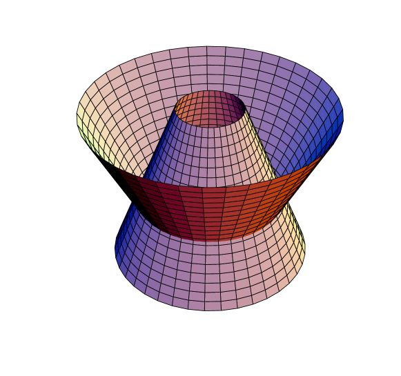
Figure 1: Crossing shells

where one spherical coordinate is suppressed and the spheres are drawn as one-dimensional circles.

Let us introduce a local coordinate system $(v,x^{A},u)$ around $S_{\times}$, such that $N_{u}:=\{u=u_{0}\}$ is the first shell and $N_{v}:=\{v=v_{0}\}$ is a second one. Hence $S_{\times}=N_{u}\cap N_{v}$. The metric takes the form similar to (77) but now both (transversal to $S_{\times}$) coordinates $u$ and $v$ are null, i.e. corresponding level three-surfaces are degenerate. More precisely,

$${g}_{\mu\nu}=\left[\begin{array}[]{ccccc}n^{A}n_{A}&\vline&n_{A}&\vline&sM+m^{A}n_{A}\\ &\vline&&\vline&\\ \hline\cr&\vline&&\vline&\\ n_{A}&\vline&g_{AB}&\vline&m_{A}\\ &\vline&&\vline&\\ \hline\cr&\vline&&\vline&\\ sM+m^{A}n_{A}&\vline&m_{A}&\vline&m^{A}m_{A}\\ \end{array}\right]$$ (49)

which gives $\sqrt{|\det g_{\mu\nu}|}=\lambda M$, and the contravariant four-metric takes the form

$${g}^{\mu\nu}=\left[\begin{array}[]{ccccc}0&\vline&-s\frac{m^{A}}{M}&\vline&\frac{s}{M}\\ &\vline&&\vline&\\ \hline\cr&\vline&&\vline&\\ -s\frac{m^{A}}{M}&\vline&{\tilde{\tilde{g}}}^{AB}+s\frac{n^{A}m^{B}+m^{A}n^{B}}{M}&\vline&-s\frac{n^{A}}{M}\\ &\vline&&\vline&\\ \hline\cr&\vline&&\vline&\\ \frac{s}{M}&\vline&-s\frac{n^{A}}{M}&\vline&0\\ \end{array}\right]\ ,$$ (50)

where $M>0$, $s:=\mathop{\rm sgn}\nolimits g^{uv}=\pm 1$, $g_{AB}$ is the induced two-metric on surfaces $\{u={\rm const},\;v={\rm const}\}$ and ${\tilde{\tilde{g}}}^{AB}$ is its inverse (contravariant) metric. Both ${\tilde{\tilde{g}}}^{AB}$ and $g_{AB}$ are used to rise and lower indices $A,B=1,2$ of the two-vectors $n^{A}$ and $m^{A}$.

Let us choose the null vector fields

$$K:=\partial_{v}-n^{A}\partial_{A}\quad\mbox{and}\quad L:=\partial_{u}-m^{A}\partial_{A}$$

which are tangent to $N_{u}$ or $N_{v}$ respectively and $g(K,L)=sM$. We can use the coordinates $(v,x^{A})$ on the first shell $N_{u}$. On the second shell $N_{v}$ we have the coordinate system $(x^{A},u)$. The canonical vector field $I$ is well defined on both shells:

$$I(K)=-\frac{K}{M}[L(\ln\lambda)]_{u}\;,\quad I(L)=-\frac{L}{M}[K(\ln\lambda)]_{v}\;,$$ (51)

where the index $u$ or $v$ corresponds to jump across first or second shell respectively.

Several continuity properties of discontinuities across $S_{\times}$ are implied by the observation that jump of the jump vanishes which we explain below on the example of a real function of two variables.
Let $f$ be a function on an open set $U\subset{\mathbb{R}}^{2}$ containing point $(0,0)$ such that $f$ is smooth outside axes (corresponding to our crossing shells), i.e. $f\in C^{k}(U^{\prime})$ for sufficiently large $k\geq 2$ and

$$\color[rgb]{1,0,0}U^{\prime}:=U\setminus(\{(x,y)\in{\mathbb{R}}^{2}\;|\;x=0\}\cup\{(x,y)\in{\mathbb{R}}^{2}\;|\;y=0\})\;.$$

Moreover, we assume that $f$ is continuous across the axes with finite jumps of first normal derivatives. More precisely, the jump

$$\left[\frac{\partial f}{\partial x}\right]_{x}:=\lim_{x\rightarrow 0^{+}}\frac{\partial f}{\partial x}(x,y)-\lim_{x\rightarrow 0^{-}}\frac{\partial f}{\partial x}(x,y)$$

is well defined for $y\neq 0$ and splits into upper (positive $y$) and lower (negative $y$) parts. Under above assumptions we get

Lemma 4.1.

The jump $\left[\frac{\partial f}{\partial x}\right]_{x}$ is continuous across $(0,0)$, i.e.

$$\lim_{y\rightarrow 0^{+}}\left[\frac{\partial f}{\partial x}\right]_{x}(y)=\lim_{y\rightarrow 0^{-}}\left[\frac{\partial f}{\partial x}\right]_{x}(y)$$

and the similar property holds on $x$-axis.

Proof.

Let us enumerate the quadrants of the plane: I, II, III, IV, i.e. $\mbox{I}\longrightarrow\{(x,y)\in{\mathbb{R}}^{2}\;|\;x>0,y>0\}$, $\mbox{II}\longrightarrow\{(x,y)\in{\mathbb{R}}^{2}\;|\;x<0,y>0\}$, $\mbox{III}\longrightarrow\{(x,y)\in{\mathbb{R}}^{2}\;|\;x<0,y<0\}$, $\mbox{IV}\longrightarrow\{(x,y)\in{\mathbb{R}}^{2}\;|\;x>0,y<0\}$, and the corresponding restrictions of the function $f$ we denote by index e.g. the function $f$ in the second quadrant we denote by $f^{II}$. Continuity of $f$ and its tangent derivatives across positive $y$-half-axis implies $f^{I}(0,y)=f^{II}(0,y)$ and $\frac{\partial^{n}f}{\partial y}^{I}(0,y)=\frac{\partial^{n}f}{\partial y}^{II}(0,y)$ $n=1,2,\ldots k$, where the boundary values of $f$ and its derivatives are defined in an obvious way e.g. $f^{I}(0,y)=\lim_{x\rightarrow 0^{+}}f^{I}(x,y)$. In particular, we have

$$\frac{\partial f}{\partial y}^{I}(0,y)=\frac{\partial f}{\partial y}^{II}(0,y)\quad\mbox{for}\;y>0\,,$$

$$\frac{\partial f}{\partial y}^{IV}(0,y)=\frac{\partial f}{\partial y}^{III}(0,y)\quad\mbox{for}\;y<0\,.$$

Passing to the limit at $(0,0)$, we get

$$\frac{\partial f}{\partial y}^{I}(0,0):=\lim_{y\rightarrow 0^{+}}\frac{\partial f}{\partial y}^{I}(0,y)=\lim_{y\rightarrow 0^{+}}\frac{\partial f}{\partial y}^{II}(0,y)=:\frac{\partial f}{\partial y}^{II}(0,0)$$

and similarly

$$\frac{\partial f}{\partial y}^{IV}(0,0):=\lim_{y\rightarrow 0^{-}}\frac{\partial f}{\partial y}^{IV}(0,y)=\lim_{y\rightarrow 0^{-}}\frac{\partial f}{\partial y}^{III}(0,y)=:\frac{\partial f}{\partial y}^{III}(0,0)\;.$$

Finally, from the last two equations we get

$$\frac{\partial f}{\partial y}^{I}(0,0)-\frac{\partial f}{\partial y}^{IV}(0,0)=\frac{\partial f}{\partial y}^{II}(0,0)-\frac{\partial f}{\partial y}^{III}(0,0)$$

which implies continuity of jump $\displaystyle\left[\frac{\partial f}{\partial x}\right]_{x}$ across $y=0$. ∎

We can denote symbolically the result as $\displaystyle\left[\left[\frac{\partial f}{\partial x}\right]_{x}\right]_{y}=0$, i.e. jump of the jump at the crossing point vanishes.

Using Lemma 4.1 one can show the following

Theorem 1.

The continuity of the metric across null shells implies that the vector fields $I(K)$ and $I(L)$ are continuous across $S_{\times}$.

Moreover, from Lemma 4.1 we get that ${\bf G}^{a}{{}_{b}}(K)$ on $N_{u}$ and ${\bf G}^{a}{{}_{b}}(L)$ on $N_{v}$ are also continuous across $S_{\times}$.

Proof.

From definition (51) of the null field $K$ and (49) we have

$$I(K)=-\frac{K}{M\lambda}[\partial_{u}\lambda]_{u}\;,$$

hence we apply Lemma 4.1 for the function $\lambda$. More precisely, we take

$$f(x,y):=\lambda(u=x+u_{0},v=y+v_{0},x^{A})$$

with fixed coordinates $x^{A}$, hence the point $x=0,y=0$ corresponds to the fixed point on $S_{\times}$ with coordinates $x^{A}$.

For ${\bf G}^{a}{{}_{b}}(K)$ we observe that

$${\bf G}^{a}{{}_{b}}(K)=s\Lambda^{a}[w_{b}]=\frac{\lambda}{2M}K^{a}K^{c}[\partial_{u}g_{cb}]_{u}$$

which is implied by (B) and (90)-(91). Moreover, from (91) we get $[w_{v}]=n^{A}[w_{A}]$, hence it is enough to consider

$$[w_{A}]=\frac{s}{2M}g_{AB}[\partial_{u}n^{B}]_{u}$$

implied by (90), and using Lemma 4.1 for the function $f:=n^{B}$ we obtain the result. ∎

The above Theorem and the considerations from Section 2 imply that the dynamics of crossing shells is described by equations (36) and (37) which hold on both shells plus continuity property across $S_{\times}$.

4.1 Spherically symmetric shells

Proposition 5.

For spherically symmetric null shell the tensor density $\;{\bf G}^{a}{{}_{b}}$ is vanishing.

This implies that the dynamics of the spherical shell is very simple, i.e. $\tau^{a}{{}_{b}}=0$, hence eqs. (36)-(37) are trivially satisfied but vector field $I$ is not vanishing as we show in the sequel.

Proof.

From (27), (B) and (91) we get

$${{\bf G}^{a}}_{b}=[{Q}^{a}_{\ b}]=\Lambda^{a}[w_{b}]$$ (52)

but spherical symmetry gives $[w_{A}]=0$ and, moreover, (91) implies $[w_{0}]=0$. ∎

Let us check the value of $I$ for the spherical null shell which arises from matching two Schwarzschild metrics along spherically symmetric null surface.

$$g_{i}=-\left(1-\frac{2m_{i}}{r_{i}}\right){\rm d}u^{2}-2{\rm d}u{\rm d}r_{i}+r_{i}^{2}{\rm d}\Omega\;,\quad i=1,2\,,$$ (53)

where

$${\rm d}\Omega:={\rm d}\theta^{2}+\sin^{2}\theta{\rm d}\varphi^{2}\;.$$

We take $u\geq 0$ for $g_{1}$ and $u\leq 0$ for $g_{2}$, and $r_{i}(R,u):=R+\frac{m_{i}}{r}u$. This implies that the full metric is continuous in coordinates $(u,R)$ across the shell $u=0$. More precisely,

$$g_{1}\bigr{|}_{u=0}=-\left(1-\frac{2m_{1}}{R}\right){\rm d}u^{2}-2{\rm d}u\left({\rm d}R+\frac{m_{1}}{R}{\rm d}u\right)+R^{2}{\rm d}\Omega=-{\rm d}u^{2}-2{\rm d}u{\rm d}R+R^{2}{\rm d}\Omega=$$

$$=-\left(1-\frac{2m_{2}}{R}\right){\rm d}u^{2}-2{\rm d}u\left({\rm d}R+\frac{m_{2}}{R}{\rm d}u\right)+R^{2}{\rm d}\Omega=g_{2}\bigr{|}_{u=0}\;.$$

Moreover, if we choose null field $X=\frac{\partial}{\partial R}$ then the transversal field may be chosen as $Y=-\frac{\partial}{\partial u}$ and $\lambda=r_{i}^{2}\sin\theta$, hence

$$Y(\ln\lambda)\bigr{|}_{u=0}=-2\frac{\partial}{\partial u}\ln\left(R+\frac{m_{i}}{R}u\right)\bigr{|}_{u=0}=-\frac{2m_{i}}{R^{2}}$$

and finally

$$I=2\frac{m_{1}-m_{2}}{R^{2}}X\,.$$ (54)

Next, for crossing two spherical null shells we may check the Dray–t’Hooft–Redmount formula [6], [25] as follows: firstly we apply Theorem 1 which from continuity of the metric implies continuity of the vector field $I$, secondly we check that the vector field $I$ is continuous through the crossing sphere iff the Dray–t’Hooft–Redmount formula is true.

Theorem 2.

If the shells are spherically symmetric than continuity of the vector field $I$ gives Dray–t’Hooft–Redmount formula (61).

Proof.

Let us consider the full description of crossing spherically symmetric null shells which can be nicely given in Kruskal–Szekeres coordinates (instead of Eddington–Finkelstein used in (53)). We assume four domains (cf. Fig. 2) equipped with the Schwarzschild metrics

$$g_{i}=-\frac{32m_{i}^{3}}{r_{i}}\exp\left(-\frac{r}{2m_{i}}\right){\rm d}u_{i}{\rm d}v_{i}+r_{i}^{2}{\rm d}\Omega\;,\quad i=1,2,3,4\,,$$ (55)

where $r_{i}=2m_{i}\kappa(-u_{i}v_{i})$ and the Kruskal function $\kappa$ is defined by its inverse $\kappa^{-1}(x)=(x-1)e^{x}$ on the interval $(0,\infty)\subset{\mathbb{R}}$. One can easily check the following identity for the first derivative of $\kappa$:

$$\kappa^{\prime}=\frac{\exp(-\kappa)}{\kappa}\,.$$ (56)

The four domains $M_{i}$ ($i=1,2,3,4$) are matched together along null surfaces $\{x\in M_{i}\;|\;u_{i}=\alpha_{i}\}\subset M_{i}$ and $\{x\in M_{i}\;|\;v_{i}=\beta_{i}\}\subset M_{i}$, as is shown on Fig. 2.

Figure 2: Matching domains

The coordinates $v_{1}$, $v_{4}$ on the shell $N_{14}$ do not match but

$$r=2m_{1}\kappa(-\alpha_{1}v_{1})=2m_{4}\kappa(-\alpha_{4}v_{4})$$ (57)

is the same on both sides and can be chosen as a coordinate on the surface $N_{14}$. This equality also means that $\lambda$ is continuous across this shell. On the other hand the continuity of the term $\frac{32m_{i}^{3}}{r_{i}}\exp\left(-\frac{r}{2m_{i}}\right){\rm d}u_{i}{\rm d}v_{i}$ across $N_{14}$ implies

$$\frac{m_{1}^{3}}{r}\exp\left(-\frac{r}{2m_{1}}\right){\rm d}u_{1}{\rm d}v_{1}\Bigr{|}_{u_{1}=\alpha_{1}}=\frac{m_{4}^{3}}{r}\exp\left(-\frac{r}{2m_{4}}\right){\rm d}u_{4}{\rm d}v_{4}\Bigr{|}_{u_{4}=\alpha_{4}}\;,$$

hence using (56) and (57) we obtain the transformation law between first derivatives of coordinates $u_{1}$ and $u_{4}$:

$$\frac{du_{4}}{du_{1}}=\left(\frac{m_{1}}{m_{4}}\right)^{3}\exp\left(-\frac{r}{2m_{1}}\right)\exp\left(\frac{r}{2m_{4}}\right)\frac{dv_{1}}{dv_{4}}=\frac{m_{1}\alpha_{4}}{m_{4}\alpha_{1}}\;.$$ (58)

Moreover, the null vector field $X$ tangent to the first shell can be represented in $M_{1}$ as follows:

$$X=\frac{\partial}{\partial r}=\left(\frac{dr}{dv_{1}}\right)^{-1}\frac{\partial}{\partial v_{1}}\;,$$

and using (56) we have

$$\frac{dr}{dv_{1}}=-2m_{1}\alpha_{1}\kappa^{\prime}(-\alpha_{1}v_{1})=-2m_{1}\alpha_{1}\left(\kappa(-\alpha_{1}v_{1})\exp[\kappa(-\alpha_{1}v_{1})]\right)^{-1}\;,$$

hence

$$X=-\frac{\kappa(-\alpha_{1}v_{1})\exp(\kappa(-\alpha_{1}v_{1}))}{2\alpha_{1}m_{1}}\frac{\partial}{\partial v_{1}}\;.$$

The transversal vector field

$$Y=\frac{\alpha_{1}}{4m_{1}}\frac{\partial}{\partial u_{1}}$$

fulfills normalization condition $g_{1}(X,Y)=1$. Moreover, using equality

$$Y(\ln\lambda)=\frac{\alpha_{1}}{2m_{1}r_{1}}\frac{\partial r_{1}}{\partial u_{1}}=\frac{r_{1}-2m_{1}}{r_{1}^{2}}$$

and the similar one in $M_{4}$ we can check the formula (54) in new coordinate representation

$$I_{14}=-[Y(\ln\lambda)]X=\frac{2m_{1}-2m_{4}}{r^{2}}X\,.$$

Similar considerations for the first shell $N_{23}$ give the following expression for the vector field (45):

$$I_{23}=\frac{2m_{2}-2m_{3}}{r^{2}}X\,,$$

where now $r=2m_{2}\kappa(-\alpha_{2}v_{2})=2m_{3}\kappa(-\alpha_{3}v_{3})$ and

$$X=\frac{\partial}{\partial r}=-\frac{\kappa(-\alpha_{2}v_{2})\exp(\kappa(-\alpha_{2}v_{2}))}{2\alpha_{2}m_{2}}\frac{\partial}{\partial v_{2}}=-\frac{\kappa(-\alpha_{3}v_{3})\exp(\kappa(-\alpha_{3}v_{3}))}{2\alpha_{3}m_{3}}\frac{\partial}{\partial v_{3}}\,.$$

We can compare $I_{14}$ with $I_{23}$ across $S_{\times}$ by using the transformation law (cf. (58)) between $v_{4}$ and $v_{3}$

$$\frac{dv_{4}}{dv_{3}}=\frac{\beta_{4}m_{3}}{\beta_{3}m_{4}}$$ (59)

which is implied by continuity of the metrics $g_{3}$ and $g_{4}$ across second shell $N_{34}$ ($v_{3}=\beta_{3}$ and $v_{4}=\beta_{4}$). Finally, we obtain

$$I_{23}(v_{3}=\beta_{3}) = -\frac{2(m_{2}-m_{3})}{r^{2}}\frac{\kappa(-\alpha_{3}\beta_{3})\exp(\kappa(-\alpha_{3}\beta_{3}))}{2\alpha_{3}m_{3}}\frac{\partial}{\partial v_{3}}$$

$$= -\frac{2(m_{2}-m_{3})}{r^{2}}\frac{\frac{r}{2m_{3}}\exp(\frac{r}{2m_{3}})}{2\alpha_{3}m_{3}}\frac{\beta_{4}m_{3}}{\beta_{3}m_{4}}\frac{\partial}{\partial v_{4}}$$

$$= -\frac{(m_{2}-m_{3})\beta_{4}\exp(\frac{r}{2m_{3}})}{2r\alpha_{3}\beta_{3}m_{4}m_{3}}\frac{\partial}{\partial v_{4}}$$

and

$$I_{14}(v_{4}=\beta_{4})=-\frac{2(m_{1}-m_{4})}{r^{2}}\frac{\frac{r}{2m_{4}}\exp(\frac{r}{2m_{4}})}{2\alpha_{4}m_{4}}\frac{\partial}{\partial v_{4}}\,,$$

hence $I_{23}=I_{14}$ on $S_{\times}$ implies

$$\frac{(m_{1}-m_{4})\exp(\frac{r}{2m_{4}})}{2r\alpha_{4}m_{4}}=\frac{(m_{2}-m_{3})\beta_{4}\exp(\frac{r}{2m_{3}})}{2r\alpha_{3}\beta_{3}m_{3}}\,,$$

or

$$(m_{1}-m_{4})\alpha_{3}\beta_{3}m_{3}\exp(-\frac{r}{2m_{3}})=(m_{2}-m_{3})\alpha_{4}\beta_{4}m_{4}\exp(-\frac{r}{2m_{4}})\,.$$ (60)

Moreover, on $S_{\times}$

$$\alpha_{i}\beta_{i}\exp(-\frac{r}{2m_{i}})=1-\kappa(-\alpha_{i}\beta_{i})=1-\frac{r}{2m_{i}}$$

which applied to (60) gives

$$(m_{1}-m_{4})(r-2m_{3})=(m_{2}-m_{3})(r-2m_{4})\,,$$

which is equivalent to Dray–t’Hooft–Redmount formula

$$(r-2m_{1})(r-2m_{3})=(r-2m_{2})(r-2m_{4})\,.$$ (61)

∎

In the above proof we have restricted ourselves to the case of positive masses $m_{i}$ and to the matching null surfaces which are not horizons. The analysis of possible special cases one can find in [11] but obviously the formula (61) remains valid for any special case.

Appendix A Transformation rules

The triad $(X,\partial_{A})$ on $S$ depends upon a particular $(2+1)$-decomposition of $S$, given by the choice of the time coordinate $x^{0}$ on $S$. However, several objects constructed by means of the triad do not depend upon this choice and describe the geometry of $S$. To prove this independence, observe that we have the following transformation law:

$${\tilde{X}} = cX\ ,$$ (62)

$${\tilde{\partial}}_{\tilde{B}} = C_{\tilde{B}}^{\ A}\partial_{A}+f_{{\tilde{B}}}X\ ,$$ (63)

where $({\tilde{X}},{\tilde{\partial}}_{\tilde{B}})$ is the new triad, corresponding to the new coordinate system $(\tilde{x}^{\tilde{a}})$ on $S$. The coefficient $c$ may be obtained from the following equation:

$$1=\langle d\tilde{x}^{0},\tilde{X}\rangle = \langle\frac{\partial\tilde{x}^{0}}{\partial x^{A}}dx^{A}+\frac{\partial\tilde{x}^{0}}{\partial x^{0}}dx^{0},cX\rangle$$ (64)

$$= c\left(-\frac{\partial\tilde{x}^{0}}{\partial x^{A}}n^{A}+\frac{\partial\tilde{x}^{0}}{\partial x^{0}}\right)\ ,$$

hence,

$$c=\left(\frac{\partial\tilde{x}^{0}}{\partial x^{0}}-\frac{\partial\tilde{x}^{0}}{\partial x^{A}}n^{A}\right)^{-1}\ .$$ (65)

On the other hand, we have:

$$\partial_{\tilde{B}} = \frac{\partial x^{A}}{\partial\tilde{x}^{\tilde{B}}}\partial_{A}+\frac{\partial x^{0}}{\partial\tilde{x}^{\tilde{B}}}\left(X+n^{A}\partial_{A}\right)$$ (66)

$$= \left(\frac{\partial x^{A}}{\partial\tilde{x}^{\tilde{B}}}+\frac{\partial x^{0}}{\partial\tilde{x}^{\tilde{B}}}n^{A}\right)\partial_{A}+\frac{\partial x^{0}}{\partial\tilde{x}^{\tilde{B}}}X\ ,$$

hence,

$$C_{\tilde{B}}^{\ A} = \frac{\partial x^{A}}{\partial\tilde{x}^{\tilde{B}}}+\frac{\partial x^{0}}{\partial\tilde{x}^{\tilde{B}}}n^{A}\ ,$$ (67)

$$f_{\tilde{B}} = \frac{\partial x^{0}}{\partial\tilde{x}^{\tilde{B}}}\ .$$ (68)

The transformation law for $g_{AB}$:

$$g_{\tilde{A}\tilde{B}}=C_{\tilde{A}}^{\ A}C_{\tilde{B}}^{\ B}g\left(\partial_{A}+f_{A}X,\partial_{B}+f_{B}X\right)=C_{\tilde{A}}^{\ A}C_{\tilde{B}}^{\ B}g_{AB}$$ (69)

implies:

$$\tilde{\lambda}=\lambda\det C_{\tilde{A}}^{\ B}\ .$$ (70)

In order to complete the triad $(X,\partial_{A})$ on $S$ to a tetrad in $M$ it is useful to choose a transverse field $Y$ fulfilling the following “normalization conditions”:

$$g(Y,X) = 1\ ,$$ (71)

$$g(Y,\partial_{A}) = 0\ .$$ (72)

These equations do not determine $Y$ uniquely, but modulo an additive term proportional to $X$: a “gauge transformation”

$$Y\rightarrow Y+hX\ ,$$ (73)

with an arbitrary scalar field $h$ is always possible. Extending coordinate $x^{0}$ from $S$ to a neighbourhood of $S$, we may choose the following transverse field:

$$Y=\frac{s}{M}\left(\partial_{3}-m^{A}\partial_{A}\right)\ .$$ (74)

We stress, however, that this particular choice of $Y$ depends not only upon a $(2+1)$-decomposition of $S$, but also on a $(3+1)$-decomposition of $M$ in a neighbourhood of $S$. Because of (72), the vectors $X$ and $Y$ span the bundle of vectors normal to $S$.

The transformation law for $Y$, when passing from one to another $(2+1)$-decomposition of $S$, reads:

$${\tilde{Y}} = c^{-1}\left(Y-k^{A}\partial_{A}\right)+hX\ ,$$ (75)

where the scalar field $h$ is arbitrary (it is determined by the extension of the $(2+1)$-decomposition of $S$ to a $(3+1)$-decomposition of $M$), and the coefficients $k^{A}$ are uniquely determined by equation

$$f_{{\tilde{B}}}=C_{\tilde{B}}^{\ A}g_{AC}k^{C}\ ,$$ (76)

with $f_{{\tilde{B}}}$ given by (68). Despite of the freedom in choice of $Y$, some geometric objects constructed with help of the tetrad $(X,\partial_{A},Y)$ do not depend upon this choice and characterize only the geometry of $S\subset M$.

Appendix B Structure of the singular Einstein tensor

We are going to relate the coordinate-dependent quantity ${\widetilde{Q}}^{\mu\nu}$ with the external curvature $Q^{a}{{}_{b}}$ of $S$. We use the form of the metric introduced in [16]:

$${g}_{\mu\nu}=\left[\begin{array}[]{ccccc}n^{A}n_{A}&\vline&n_{A}&\vline&sM+m^{A}n_{A}\\ &\vline&&\vline&\\ \hline\cr&\vline&&\vline&\\ n_{A}&\vline&g_{AB}&\vline&m_{A}\\ &\vline&&\vline&\\ \hline\cr&\vline&&\vline&\\ sM+m^{A}n_{A}&\vline&m_{A}&\vline&\left(\frac{M}{N}\right)^{2}+m^{A}m_{A}\\ \end{array}\right]\ ,$$ (77)

and

$${g}^{\mu\nu}=\left[\begin{array}[]{ccccc}-\left(\frac{1}{N}\right)^{2}&\vline&\frac{n^{A}}{N^{2}}-s\frac{m^{A}}{M}&\vline&\frac{s}{M}\\ &\vline&&\vline&\\ \hline\cr&\vline&&\vline&\\ \frac{n^{A}}{N^{2}}-s\frac{m^{A}}{M}&\vline&{\tilde{\tilde{g}}}^{AB}-\frac{n^{A}n^{B}}{N^{2}}+s\frac{n^{A}m^{B}+m^{A}n^{B}}{M}&\vline&-s\frac{n^{A}}{M}\\ &\vline&&\vline&\\ \hline\cr&\vline&&\vline&\\ \frac{s}{M}&\vline&-s\frac{n^{A}}{M}&\vline&0\\ \end{array}\right]\ ,$$ (78)

where $M>0$, $s:=\mathop{\rm sgn}\nolimits g^{03}=\pm 1$, $g_{AB}$ is the induced two-metric on surfaces $\{x^{0}={\rm const},\;x^{3}={\rm const}\}$ and ${\tilde{\tilde{g}}}^{AB}$ is its inverse (contravariant) metric. Both ${\tilde{\tilde{g}}}^{AB}$ and $g_{AB}$ are used to rise and lower indices $A,B=1,2$ of the two-vectors $n^{A}$ and $m^{A}$.

Formula (77) implies: $\sqrt{|\det g_{\mu\nu}|}=\lambda M$. Moreover, the object $\Lambda^{a}$ defined by formula (3), takes the form $\Lambda^{a}=\lambda X^{a}$, where $\lambda$ is given by formula (2) and $X:=\partial_{0}-n^{A}\partial_{A}$. This means that we have chosen the following degeneracy field: $X^{\mu}=(1,-n^{A},0)$.

For calculational purposes it is useful to rewrite the two-dimensional inverse metric ${\tilde{\tilde{g}}}^{AB}$ in three-dimensional notation, putting ${\tilde{\tilde{g}}}^{0a}:=0$. This object satisfies the obvious identity:

$${\tilde{\tilde{g}}}^{ac}g_{cb}=\delta^{a}{{}_{b}}-X^{a}\delta^{0}{{}_{b}}\,.$$

Hence, the contravariant metric (78) may be rewritten as follows:

$$g^{ab}={\tilde{\tilde{g}}}^{ab}-\frac{1}{N^{2}}X^{a}X^{b}-\frac{s}{M}(m^{a}X^{b}+m^{b}X^{a})\ ,$$ (79)

where $m^{a}:={\tilde{\tilde{g}}}^{aB}m_{B}$, so that $m^{0}:=0$, and

$$g^{3\mu}=\frac{s}{M}X^{\mu}\ .$$

It may be easily checked (see, e.g., [16], page 406) that covariant derivatives of the field $X$ along $S$ are equal to:

$$\nabla_{a}X=-w_{a}X-l_{ab}{\tilde{\tilde{g}}}^{bc}\partial_{c}\ ,$$ (80)

where

$$w_{a}:=-X^{\mu}\Gamma^{0}_{\mu a}\ ,$$ (81)

and

$$l_{ab}:=-g(\partial_{b},\nabla_{a}X)=g(\nabla_{a}\partial_{b},X)=X_{\mu}\Gamma^{\mu}_{ab}\ .$$ (82)

Moreover,

$$\partial_{c}\Lambda^{c}= -\lambda g^{ab}l_{ab}=-\lambda{\tilde{\tilde{g}}}^{ab}l_{ab}=-\lambda l\ ,$$ (83)

where $l={\tilde{\tilde{g}}}^{ab}l_{ab}$.

The following lemma was proved in [17]:

Lemma B.1.

The object ${{\widetilde{Q}}}^{a}{{}_{b}}$ is related to $Q^{a}{{}_{b}}$ as follows:

$$s{{\widetilde{Q}}}^{a}{{}_{b}}=sQ^{a}{{}_{b}}-\frac{1}{2}\lambda l\delta^{a}{{}_{b}}+\Lambda^{a}\chi_{b}-\delta^{a}{{}_{b}}\Lambda^{c}\chi_{c}\ ,$$ (84)

where $\displaystyle\chi_{c}:=\frac{1}{2}\partial_{c}\ln\left(\frac{M}{\lambda}\right)$.

Moreover, from definition (17) and property (80) one can check that

$$sQ^{a}{{}_{b}} = \lambda\delta^{a}{{}_{b}}\nabla_{c}X^{c}-\lambda\nabla_{b}X^{a}-\delta^{a}{{}_{b}}\partial_{c}\Lambda^{c}$$ (85)

$$= -\lambda\delta^{a}{{}_{b}}(w_{c}X^{c}+l)+\lambda(w_{b}X^{a}+{\tilde{\tilde{g}}}^{ac}l_{cb})+\delta^{a}{{}_{b}}\lambda l$$

$$= \lambda{\tilde{\tilde{g}}}^{ac}l_{cb}+\Lambda^{a}w_{b}-\delta^{a}{{}_{b}}\Lambda^{c}w_{c}\,.$$

Remark: Formula (85), together with $l_{ab}X^{b}=0=g_{ab}X^{b}$, gives us the orthogonality condition $Q^{a}{{}_{b}}X^{b}=0$ and symmetry of the tensor $Q_{ab}:=g_{ac}Q^{c}{{}_{b}}$.

Now, we would like to examine the properties of ${\bf G}^{\mu\nu}=[{\widetilde{Q}}^{\mu\nu}]$. From continuity of the metric across $S$ we obtain

$$[l_{ab}]=sM[A^{3}_{ab}]=sM[\Gamma^{3}_{ab}]=X^{c}[\Gamma_{cab}]=0\,,$$ (86)

$$s[{{\widetilde{Q}}}^{a}{{}_{b}}] =\Lambda^{a}[A^{3}_{3b}]-\delta^{a}{{}_{b}}\Lambda^{c}[A^{3}_{3c}]$$

$$=\Lambda^{a}[w_{b}]-\delta^{a}{{}_{b}}\Lambda^{c}[w_{c}]=s[Q^{a}{{}_{b}}]\ ,$$ (87)

and

$$[{{\widetilde{Q}}}^{3}{{}_{\mu}}]=0\$$ (88)

because $s{{\widetilde{Q}}}^{3}{{}_{3}}=-\frac{1}{2}\lambda l$ and $s{{\widetilde{Q}}}^{3}{{}_{a}}=0$.

Finally, the missing component $[{\widetilde{Q}}^{a}{{}_{3}}]$ has the following form:

$$[{\widetilde{Q}}^{a}{{}_{3}}]=s\Lambda^{a}\left\{-[\partial_{3}\ln\lambda]+m^{b}[w_{b}]\right\}+M\lambda{\tilde{\tilde{g}}}^{ab}[w_{b}]\,.$$ (89)

We also have from

$$[w_{a}]=-X^{b}g^{03}[\Gamma_{3\,ba}]=\frac{s}{2M}X^{b}[g_{ab,3}]$$ (90)

that

$$X^{a}[w_{a}]=\frac{s}{2M}[X^{a}X^{b}g_{ab,3}]=0\,.$$ (91)

Using these results from (88) one can easily check the property (21)

$${\bf G}^{33}=[{\widetilde{Q}}^{33}] = g^{33}[{\widetilde{Q}}^{3}{{}_{3}}]+g^{3b}[{\widetilde{Q}}^{3}{{}_{b}}]=0\ ,$$

$${\bf G}^{3a}=[{\widetilde{Q}}^{3a}] = g^{33}[{\widetilde{Q}}^{a}{{}_{3}}]+g^{3b}[{\widetilde{Q}}^{a}{{}_{b}}]=-\frac{s}{M}[X^{b}Q^{a}{{}_{b}}]=0\ ,$$

where we used the equality $[{\widetilde{Q}}^{a}{{}_{b}}]=[Q^{a}{{}_{b}}]$ which is crucial to admit that the object ${\bf G}^{a}{{}_{b}}$ is a well defined geometric object on $S$.

Appendix C Gauss–Codazzi equations

It was shown in [17] that

$$s{\cal G}^{3}_{\ a}= -s\partial_{b}{Q}^{b}{{}_{a}}+\frac{1}{2}s{Q}^{bc}g_{bc,a}+\lambda\partial_{a}l\ ,$$ (92)

where we have used the formula

$$sQ^{ab}=\lambda{\tilde{\tilde{g}}}^{ac}{\tilde{\tilde{g}}}^{bd}l_{cd}+(\Lambda^{a}{\tilde{\tilde{g}}}^{bc}+\Lambda^{b}{\tilde{\tilde{g}}}^{ac}-{\tilde{\tilde{g}}}^{ab}\Lambda^{c})w_{c}\,.$$

References

• [1] R. Arnowitt, S. Deser, and C. Misner, in Gravitation: an Introduction to Current Research, edited by L. Witten (Wiley, New York, 1962), p. 227.
• [2] A. Ashtekar, C. Beetle and J. Lewandowski, Class. Quantum Grav. 19, 1195–1225 (2002)
• [3] C. Barrabès and W. Israel, Phys. Rev. D 43, 1129 (1991).
• [4] F. J. Belinfante, Physica 6, 887 (1939); 7, 449 (1940); L. Rosenfeld, Acad. Roy. Belg. 18, 1 (1940).
• [5] P. A. M. Dirac, Proc. Roy. Soc. London, Ser. A 268 (1962) 57.
• [6] T. Dray and G. t’Hooft, Commun. Math. Phys. 99 (1985) 613.
• [7] P. Hájíček, B. S. Kay, and K. Kuchař, Phys. Rev. D 46, 5439 (1992).
• [8] P. Hájíček and J. Kijowski, Phys. Rev. D 57, 914 (1998).
• [9] P. Hájíček and J. Kijowski, Phys. Rev. D 62, 044025-1 (2001).
• [10] P. Hájíček and C. Kiefer, Nucl. Phys. B 603, 531 (2001); P. Hájíček, Nucl. Phys. B 603, 555 (2001).
• [11] P. Hájíček and I. Kouletsis, Pair of Null Gravitating Shells I. Space of Solutions and Symmetry, preprint, gr-qc/0112060.
• [12] P. Hájíček and I. Kouletsis, Pair of Null Gravitating Shells II. Canonical theory and embedding variables, preprint, gr-qc/0112061.
• [13] I. Kouletsis and P. Hájíček, Pair of Null Gravitating Shells III. Algebra of Dirac Observables, preprint, gr-qc/0112062.
• [14] P. Hájíček, Quantum theory of gravitational collapse (lecture notes on quantum conchology), preprint BUTP-02/4, lecture notes for the talk “Quantum theory of gravitational collapse” given at the 271.WE-Heraeus-Seminar “Aspects of Quantum Gravity” at Bad Honnef, 25 February–1 March 2002.
• [15] W. Israel, Nuovo Cimento B 44, 1 (1966); 48, 463 (1967) [erratum].
• [16] J. Jezierski, J. Kijowski, and E. Czuchry, Rep. Math. Phys. 46, 397 (2000).
• [17] J. Jezierski, J. Kijowski, and E. Czuchry, Phys. Rev. D 65, 064036 (2002)
• [18] J. Kijowski, Acta Phys. Pol. B 29, 1001 (1998).
• [19] J. Kijowski, in Proceedings of Journées Relativistes 1983 (Pitagora Editrice, Bologna, 1985), p. 205; in Gravitation, Geometry and Relativistic Physics, (Springer Lecture Notes in Physics, vol. 212, 1984), p. 40; Gen. Relativ. Gravit. 29, 307 (1997).
• [20] J. Kijowski, A. Smólski, and A. Górnicka, Phys. Rev. D. 41, 1875 (1990); J. Kijowski and G. Magli, J. Geometry and Phys. 9 207 (1992); Class. Quantum Grav. 15, 3891 (1998); J. Jezierski and J. Kijowski, in Nonequilibrium Theory and Extremum Principles, edited by S. Sieniutycz and P. Salamon (Taylor & Francis, N. Y. – London, 1990), p. 282.
• [21] J. Louko, B. Whiting, and J. Friedman, Phys. Rev. D 57 (1998) 2279.
• [22] M. Mars and J.M.M. Senovilla, Class. Quantum Grav. 10 (1993) 1865–1897
• [23] C. W. Misner, K. S. Thorne, and J. A. Wheeler, Gravitation, (Freeman, San Francisco, 1973).
• [24] A. Raychaudhuri, Phys. Rev. 98, 1123 (1955); S.W. Hawking, G.F.R. Ellis, The Large Scale Structure of Space-Time, (Cambridge Univ. Press, 1973)
• [25] I.H. Redmount, Prog. Theor. Phys. (1995) 1401.
• [26] J. A. Schouten, Ricci-Calculus: an Introduction to Tensor Analysis and its Geometrical Applications (Springer-Verlag, Berlin, 1954), 2nd edn, p. 102.
• [27] A. H. Taub, J. Math. Phys. 21, 1423 (1980).