Matter and dynamics in closed cosmologies

Abstract

To systematically analyze the dynamical implications of the matter content in cosmology, we generalize earlier dynamical systems approaches so that perfect fluids with a general barotropic equation of state can be treated. We focus on locally rotationally symmetric Bianchi type IX and Kantowski-Sachs orthogonal perfect fluid models, since such models exhibit a particularly rich dynamical structure and also illustrate typical features of more general cases. For these models, we recast Einstein’s field equations into a regular system on a compact state space, which is the basis for our analysis. We prove that models expand from a singularity and recollapse to a singularity when the perfect fluid satisfies the strong energy condition. When the matter source admits Einstein’s static model, we present a comprehensive dynamical description, which includes asymptotic behavior, of models in the neighborhood of the Einstein model; these results make earlier claims about “homoclinic phenomena and chaos” highly questionable. We also discuss aspects of the global asymptotic dynamics, in particular, we give criteria for the collapse to a singularity, and we describe when models expand forever to a state of infinite dilution; possible initial and final states are analyzed. Numerical investigations complement the analytical results.

PACS number(s): 04.20-q, 98.80.Jk, 98.80.Cq, 04.20.Ha

1 Introduction

At present, the matter content in the Universe is a mystery: dark matter, dark energy, quintessence; our knowledge that underlies these labels is clearly not as good as we would wish. Apart from observational challenges this also poses theoretical issues, for example, very little is known about how matter properties influence cosmological evolution, the character of singularities, and the stability of various special cosmological models. This motivates the development of a framework that is insensitive to the details of the matter content, but still allows one to systematically investigate the relationship between properties of matter and cosmological dynamics. The book edited by Wainwright and Ellis [1] used dynamical systems methods to successfully study perfect fluid models with a linear equation of state; in this paper we modify and generalize the formalism in [1], and attempt to show that the usefulness of dynamical systems methods increases with the complexity of the matter source.

In this paper we consider spatially homogeneous (SH) cosmological models with orthogonal perfect fluid matter (i.e., the fluid velocity is orthogonal with respect to the symmetry surfaces) described by an effective barotropic equation of state $p=p(\rho)$, where $p$ denotes the pressure and $\rho$ the energy-density, which we assume to be non-negative; the effective fluid may consist of an arbitrary number of non-interacting orthogonal perfect fluids with non-negative energy-densities and barotropic equations of state, and a positive cosmological constant. From these assumptions it follows that SH Bianchi type I-VIII cosmologies are forever expanding or contracting and comparatively easy to treat, as discussed in the concluding remarks. We therefore focus on SH Bianchi type IX and Kantowski-Sachs perfect fluid models which exhibit a particularly rich dynamical structure. These models are the only SH models that admit positive intrinsic curvature; they thus naturally have a closed spatial topology and we therefore refer to them as closed cosmologies (although all Bianchi class A and some class B models also admit closed spatial topologies). However, we restrict ourselves to the locally rotationally symmetric (LRS) orthogonal perfect fluid cases, since this suffices to illustrate our approach; generalizations, even to models with no symmetries at all, are discussed in the concluding remarks.

The LRS type IX and Kantowski-Sachs models have been studied before: in [2], [3], [4] dynamical systems techniques were used to study quite special sources, e.g., perfect fluids with a linear equations of state and a cosmological constant; other methods were used in [5] and [6] to treat more general matter that included perfect fluids with non-negative pressure, note however that this excludes e.g., the inclusion of a cosmological constant. Recently the dynamics associated with Einstein’s static model was studied in a series of papers that covered several special cases in a LRS type IX context: a positive cosmological constant and dust in [7], a positive cosmological constant and a perfect fluid with a linear equation of state in [8]; the latter work was subsequently generalized to the diagonal non-LRS type IX case in [9]. In these papers it was asserted that the presence of Einstein’s static model leads to the existence of infinitely many homoclinic orbits [orbits whose $\alpha$- and $\omega$-limit is the same periodic orbit] that “produce chaotic sets in the whole state space”; the asymptotic configurations of models in a neighborhood of Einstein’s model, as of any domain in the whole phase space, were claimed to be unpredictable and characterized by “homoclinic chaos.” We reach a different conclusion: we present a comprehensive description of the dynamics in the neighborhood of the Einstein model, moreover, we establish theorems about the global asymptotic behavior of solutions. Our results disprove the claims of non-predictability and chaos for models close to the Einstein model; furthermore, we prove that the asserted “homoclinic phenomena” must be confined to quite small regions of the phase space, if they occur at all; indeed, our numerical investigations suggest that “homoclinic chaos” is excluded entirely, but further studies are needed to establish this with certainty.

Our investigation is based on a reformulation of Einstein’s field equations for LRS type IX (Kantowski-Sachs) models as a completely regular dynamical system on a compact four-dimensional (three-dimensional) state space. Building on this, our analysis of the type IX case rests on three cornerstones: methods from dynamical systems theory, in particular center manifold analysis, the existence of a conserved “energy” integral, and the close relationship between the dynamics of the full system and the Friedmann-Robertson-Walker (FRW) case.

The outline of the paper is as follows: in Sec. 2, we reformulate Einstein’s field equations for the LRS type IX and Kantowski-Sachs models as a regular dynamical system on a compact state space; in type IX we also find a conserved “energy.” In Sec. 3 we describe the FRW models; first with a potential approach, presumably familiar to a general reader, and then with our dynamical systems formulation. In contrast to the potential formulation, the dynamical systems approach can be applied to more general cases. In Sec. 4 we investigate the LRS type IX models. Together with dynamical systems methods and center manifold reduction we use the conserved quantity to obtain comprehensive information about the dynamical possibilities. The dynamical system contains the Kantowski-Sachs models as an invariant boundary subset; these models are briefly treated in Sec. 5. We conclude with a discussion about other cases and how the present work fits in a larger context as regards the dynamics of quite general models in Sec. 6. Some proofs and supplementary theorems about aspects of the global dynamics are postponed to the appendix, where we also show how our variables are related to the Hubble-normalized variables used in e.g., [1]. Throughout we use units such that the speed of light $c$ and Newton’s gravitational constant $G$ are given by $c=1=8\pi G$.

2 The dynamical systems approach

The LRS Bianchi type IX models are characterized by the equations

$$\dot{H} =-H^{2}-2\sigma_{+}^{2}-{\textstyle{\frac{1}{6}}}(\rho+3p)\,, \qquad\dot{\sigma}_{+} =-3H\sigma_{+}-{{}^{3}}S_{+}\,,$$

$$\dot{n}_{1} =-(H+4\sigma_{+})n_{1}\,, \qquad\dot{n}_{2} =-(H-2\sigma_{+})n_{2}\,,$$ (1)

$$\dot{\rho} =-3(\rho+p)H\,, \qquad\rho =3H^{2}-3\sigma_{+}^{2}+{\textstyle{\frac{1}{2}}}{{}^{3}}R\ ,$$

(see p. 40, 123–124 in [1]; $n_{2}=n_{3}$, $\sigma_{-}=0$ yields the LRS case). The Hubble scalar $H$ allows one to define the length scale $\ell$ through $H=\dot{\ell}/\ell$, where $\ell$ is the cubic root of the volume density. The shear is determined by $\sigma_{+}$; $n_{1}$ and $n_{2}$ describe the spatial three-curvature via ${}^{3}R=-{\textstyle{\frac{1}{2}}}n_{1}^{2}+2n_{1}n_{2}$ and $S_{+}=\frac{1}{3}(n_{1}n_{2}-n_{1}^{2})$. The overdot denotes differentiation w.r.t. clock time $t$.

The algebraic equation for $\rho$ yields $H^{2}+\frac{1}{3}n_{1}n_{2}=\frac{1}{3}\rho+\sigma_{+}^{2}+\frac{1}{12}n_{1}^{2}$. Since $n_{1}$ and $n_{2}$ have the same sign in Bianchi type IX, we can replace $n_{2}$ with the variable $D:=(H^{2}+n_{1}n_{2}/3)^{1/2}$ . We then introduce the bounded dimensionless variables

$$\left(Q_{0},\ Q_{+}\right) :=\left(H,\ \sigma_{+}\right)/D\,, \qquad(M_{1},\Omega_{D}):=\left(n_{1}^{2},4\rho\right)/(12D^{2})\,.$$ (2)

By definition, $-1<Q_{0}<1$ and $M_{1}>0$, while $\rho>0$ implies

$$\Omega_{D}=1-Q_{+}^{2}-M_{1}>0\,.$$ (3)

We replace $H,\sigma_{+},n_{1},n_{2}$ with $Q_{0},Q_{+},M_{1},D$, and $\rho$ with $\Omega_{D}$, which is given in terms of $Q_{+}$ and $M_{1}$ by (3); instead of $p$ we introduce the dimensionless quantity $w=p/\rho$. Then (1) yields one decoupled dimensional equation

$$D^{\prime}=-D(Q_{0}F+Q_{0}+Q_{+})\,,\qquad F:=2Q_{+}^{2}-Q_{0}Q_{+}+{\textstyle{\frac{1}{2}}}(1+3w(L))\Omega_{D}\,,$$ (4)

and the coupled dimensionless system

$$\begin{array}[]{lll}Q_{0}^{\prime}&=&-(1-Q_{0}^{2})F\,,\\[3.01385pt] Q_{+}^{\prime}&=&4M_{1}-1+(Q_{0}-Q_{+})^{2}+Q_{0}Q_{+}F\,,\\[3.01385pt] M_{1}^{\prime}&=&2M_{1}(Q_{0}F-3Q_{+})\,,\\[3.01385pt] L^{\prime}&=&f(L)L(1-L)Q_{0}\,,\end{array}$$ (5)

where ${}^{\prime}=\frac{1}{d\tau}:=\frac{1}{Ddt}$ stems from a new dimensionless time variable $\tau$; the variable $L$ is discussed below. The system (5) is complemented by the auxiliary equation

$$\Omega_{D}^{\prime}=(2Q_{0}F-(1+3w)Q_{0}+2Q_{+})\Omega_{D}\>.$$ (6)

The coupled system (5) describes the essential dynamics; once solved, the metric can be obtained in terms of quadratures, cf. Ch. 10 in [1]. The r.h.s. is polynomial in $Q_{0},Q_{+},M_{1}$. This makes an inclusion of the boundary, which consists of invariant subsets, possible; $Q_{0}=\pm 1$ yields the forever expanding and contracting representations of the LRS Bianchi type II models; $M_{1}=0$ yields the Kantowski-Sachs models (see, e.g., [11]) and $\Omega_{D}=0$ the vacuum boundary. We denote the state space of (5) by

$${}^{4}\textbf{X}=\{(Q_{0},Q_{+},M_{1},L)\}\,.$$ (7)

The choice of the variable $L$ depends on the equation of state; $L$ is constructed from $\ell$ in two steps: (i) Let $x:=\ell/\ell_{0}$, where $\ell_{0}=\ell(t_{0})$ and $t_{0}$ is a fixed reference time; introduce $\lambda(x)$ subject to the conditions $\lambda(x)\in\mathcal{C}^{0}[0,\infty)$, $\lambda(x)\in\mathcal{C}^{2}(0,\infty)$, $d\lambda/dx>0$, $\lambda(0)=0$, and $\lim_{x\rightarrow\infty}\lambda(x)\rightarrow\infty$. (ii) Introduce $L:=\lambda/(1+\lambda)$; it follows that $L(x)$ is monotonically increasing, and $L\in(0,1)$ for $x>0$, thus $L\rightarrow 0$ describes a singularity while $L\rightarrow 1$ represents a state of infinite dispersion. Moreover, we define $f(L):={d\ln\lambda}/{d\ln x}|_{x(L)}$.

The function $w$ in (4) is to be regarded as a function $w(L)$: from (1) we have $d\rho/(\rho+p)=-3dx/x$, which can be integrated to yield a function $\rho(x)$ when an equation of state $p(\rho)$ is given, see also the example below. Via $x=x(L)$ this leads to $w(L):=p/\rho\,|_{x(L)}$.

The variables $n_{1,2}$ are algebraically related to the spatial metric and $H$, $\sigma_{+}$ to the extrinsic curvature (see Ch. 10 in [1]), and are hence continuous in $t$, or equivalently in $x$ and $L$; $\rho$ is continuous by virtue of (1), $Q_{0},Q_{+},M_{1},D$ are continuous through (2); however, $p$, and hence $w=p/\rho$, is not necessarily continuous – jumps in $p$ correspond to phase transitions. Although these can be covered by our formalism, we will for simplicity assume that $p(\rho)$ is at least ${\mathcal{C}}^{1}$; therefore $w(L)$ and thus the r.h.s. of (5) is ${\mathcal{C}}^{1}(0,1)$ (see [12] for related issues).

For large classes of equations of state, $L$ can be chosen so that (5) is endowed with the desirable differentiability properties for all $L\in[0,1]$, and thus the boundaries $L=0,1$ can be included. We define an equation of state to be asymptotically linear if $w\rightarrow dp/d\rho\rightarrow const\,(=w_{0},w_{1})$ when $p\rightarrow 0,\infty$. In this case we choose $L$ so that $w(L)$ and $f(L)$ become $\mathcal{C}^{1}$ on $L\in[0,1]$; thus $w(0)=w_{0}$, $w(1)=w_{1}$, $f(0)=f_{0}$, $f(1)=f_{1}$. We restrict ourselves to the situation where $f_{0}>0$ and $f_{1}>0$ is possible.

To make things less abstract, let us consider the special case of a source that consists of an arbitrary number of non-interacting perfect fluids with linear equations of state; the total energy-density is $\rho(x)=\sum_{i}\rho_{i0}x^{-3(1+w_{i})}$, where $\sum_{i}\rho_{i0}=\rho_{0}$ (the total energy-momentum $T^{\mu\nu}$ is a sum of the $T_{i}^{\mu\nu}$ for each fluid component $i$; each component satisfies ${T^{\mu\nu}_{i}}{}_{;\nu}=0$, and hence $T^{\mu\nu}{}_{;\nu}=0$). We assume that $\rho_{i0}\geq 0$ and $w_{i}\geq-1\>\,\forall\,i$; causality of each component requires $w_{i}\leq 1$. As an example of how to obtain a suitable variable $L$, let us take the combination of two fluids with $w_{0}>w_{1}$; the choice $\lambda(x)=\frac{\rho_{10}}{\rho_{00}}x^{3(w_{0}-w_{1})}$ yields $w=w_{0}-(w_{0}-w_{1})L$ and $f(L)=3(w_{0}-w_{1})$, which clearly satisfies the above conditions. As a second example, consider a source that consists of radiation, dust and a cosmological constant (a cosmological constant corresponds to ${\rho}_{\Lambda 0}=\Lambda$ and $w_{\Lambda}=-1$); a possible choice that satisfies the requirements is $\lambda=x$, which implies $f(L)=1$ and

$$w(L)=\frac{{\textstyle{\frac{1}{3}}}{\rho}_{r0}\,(1-L)^{4}-{\rho}_{\Lambda 0}L^{4}}{{\rho}_{r0}\,(1-L)^{4}+{\rho}_{d0}\,L\,(1-L)^{3}+{\rho}_{\Lambda 0}\,L^{4}}\,.$$ (8)

The dimensionless coupled dynamical system (5) is thus regular everywhere on the state space ${}^{4}\textbf{X}$, including the boundaries $Q_{0}=\pm 1$, $Q_{+}=\pm 1$, $M_{1}=0$, and $\Omega_{D}=0$; $L=0$, $L=1$ are also included when the equation of state is asymptotically linear, however, even when this is not the case, attractors and repellors are distinct sets on $L=0,1$, as we will see in the following sections.

The system (5) is invariant under the discrete transformation $(Q_{0},Q_{+},\tau)\rightarrow-(Q_{0},Q_{+},\tau)$, which is a consequence of the invariance of the field equations under time reversal. This reflects itself in the fact that the fixed points of the system appear in pairs, except for the “Einstein point” which is invariant since $Q_{0}=Q_{+}=0$, see below.

The system (5) admits the integral

$${{\mathcal{E}}}(Q_{0},Q_{+},M_{1},L):=\frac{3\,(1-Q_{0}^{2})^{4/3}\,V(L)}{4^{4/3}\,\Omega_{D}\,M_{1}^{1/3}}=E\,,$$ (9)

where $E$ is a constant “energy.” This conserved quantity is a generalization of an integral that describes the solution structure in the FRW case, cf. Sec. 3. In (9), the “potential” $V$ is defined as

$$V:=-{\tilde{\rho}}\,x^{2}\>,$$ (10)

where $\tilde{\rho}(x):=\rho/\rho_{0}$, and hence $V<0$ since $\rho>0$; $V$ can be viewed as function of $x$ and thus of $L$ via $x(L)$, and

$$\begin{array}[]{lll}dV/dL&=&-(1+3w)V[f(L)L(1-L)]^{-1}\quad\text{and}\\[1.72218pt] V^{\prime}&=&-(1+3w)VQ_{0}\,,\end{array}$$ (11)

follows from $d\tilde{\rho}/dx=-3\tilde{\rho}(1+w)x^{-1}$. Eq. (11) in combination with (5) leads to the claimed conservation of ${\mathcal{E}}$; ${\mathcal{E}}^{\prime}=0$. The integral ${\mathcal{E}}$ foliates the interior of the 4-dimensional state space ${}^{4}\textbf{X}$ into 3-dimensional hypersurfaces.

As an example of a potential $V$, consider again the combination of two fluids with $w_{0}>w_{1}$; the choice $\lambda(x)=(\rho_{10}/\rho_{00})x^{3(w_{0}-w_{1})}$ leads to

$$V(L)=-C^{2}\,\left[\,L^{-(1+3w_{0})}\,(1-L)^{1+3w_{1}}\,\right]^{1/[3(w_{0}-w_{1})]}\,,$$ (12)

with $C=C(\rho_{00},\rho_{10})=const$. The special case of a cosmological constant and a perfect fluid $p=w_{0}\rho$ results in

$$V(L)=\left[\frac{L(1-{\mathcal{L}})}{{\mathcal{L}}(1-L)}\right]^{2/[3(1+w_{0})]}\,\left(\frac{{\mathcal{L}}}{L}\right)\,V_{max}\,,$$ (13)

where $V_{max}=V({\mathcal{L}})$; ${\mathcal{L}}$ is defined by $w({\mathcal{L}})=-{\textstyle{\frac{1}{3}}}$, which in the present case yields ${\mathcal{L}}:=(w_{0}+1/3)/(1+w_{0})$.

To obtain a better feeling for our formalism we begin with a description of the FRW cosmologies; first in the potential approach, presumably familiar to a general reader, and then in the dynamical systems picture.

3 FRW cosmologies

3.1 The potential approach

FRW models are characterized by the scale factor $\ell(t)$ subject to the three key equations (see, e.g., [14])

$$\dot{\ell}^{\,2}={\textstyle{\frac{1}{3}}}\rho\ell^{2}-k\,,\,\>{\ddot{\ell}}=-{\textstyle{\frac{1}{6}}}(\rho+3p)\ell\,,\,\>{\dot{\rho}}=-3(\rho+p)\,\dot{\ell}/\ell\,,$$ (14)

where $t$ denotes the clock time along the fluid congruence which is orthogonal to the symmetry surfaces. The first equation is the Friedmann equation, which is an integral of the second one, Raychadhuri’s equation; the third equation describes local conservation of energy; $k=+1,0,-1$ determines the sign of the spatial curvature. The combinations $\rho+3p$ and $\rho+p$ can be regarded as an active gravitational and inertial mass-density, respectively; positive (negative) $\rho+3p$, i.e. $w>-1/3$ ($w<-1/3$) when $\rho>0$, implies deceleration (acceleration).

To obtain a dimensionless formulation, $\ell$ is rescaled w.r.t. a reference time $t_{0}$: $x=\ell/\ell_{0}$ (with $\ell_{0}=\ell(t_{0})$; see p. 744 of [14]). A natural choice for a dimensionless time variable is $H(t_{0})\,t$, which measures time in “Hubble units”; however, for our purposes we find it more convenient to introduce $t_{\rho}:=\sqrt{\rho_{0}/3}\>t$, i.e., we measure time in “energy-density units.” Expressed in $x$ and $t_{\rho}$, (14) takes the form

$${\dot{x}}^{2}=E-V\,,\,\,{\ddot{x}}={\textstyle{\frac{1}{2}}}(1+3w)Vx^{-1}\,,\,\,\dot{\tilde{\rho}}=-3\tilde{\rho}(1+w)\,\dot{x}/x\>,$$ (15)

where the overdot now denotes differentiation w.r.t. $t_{\rho}$. The equation of state enters via the functions $w(x)$ and $V(x)$, cf. (10); note that the potential $V$ is scaled so that $V(1)=-1$. The first equation in (15) can be interpreted as an “energy” integral

$${\mathcal{E}}={\dot{x}}^{2}+V=-(\rho-3H^{2})\ell^{2}/(\rho_{0}\ell_{0}^{2})=E\>,$$ (16)

where the constant $E$ is given by $E=-(3k)/(\rho_{0}\ell_{0}^{2})$. The problem is thus analogous to the problem of a particle with energy $E$ that moves in a potential $V(x)$. The condition $V<0$ implies that the open ($E>0$) and flat models ($E=0$) are either forever expanding or contracting; however, the qualitative behavior of closed models ($E<0$) depends on both the shape of the potential and the value of $E$; we now focus on this case.

In addition to a non-negative energy-density, we henceforth also assume a non-negative inertial mass-density $\rho+p$ (weak energy condition), i.e., $w\geq-1$ when $\rho>0$ (recall that $w=-1$ corresponds to a cosmological constant). For simplicity we also assume that there exists at most one value of $x$ such that $w(x)=-1/3$; hence we require $dw/dx\,|_{w^{-1}(-1/3)}<0$, or equivalently $dw/d\rho\,|_{w^{-1}(-1/3)}>0$. Under these assumptions $V$ has a maximum at $x=w^{-1}(-1/3)$, since $dV/dx=-(1+3w)Vx^{-1}=0$ at $x=w^{-1}(-1/3)$ and $d^{2}V/dx^{2}\,|_{w^{-1}(-1/3)}=-6\tilde{\rho}^{2}dw/d\tilde{\rho}\,|_{w=-1/3}<0$.

We distinguish five different cases; different matter assumptions yield qualitatively different dynamical properties for the associated FRW models, see Table 1; the corresponding potentials are depicted in Figs. 1, 2(a), and 2(c).

Case	$w(x)$	Qualitative FRW Dynamics
(i)	$w>-1/3$, $\inf w>-1/3$	expanding–contracting
(ii)	$w>-1/3$ for small $x$	$E=E_{1}$ : forever expanding/contracting
	$w=-1/3$ for a unique $x$	$E=E_{s}$ : expanding/contracting–Einstein static
	$w<-1/3$ for large $x$	$E=E_{2}$ : expanding–contracting or reverse
(iii)	$w<-1/3$, $\sup w<-1/3$	contracting–expanding
(iv)	$w>-1/3$ for $x\rightarrow 0$	$E=E_{1}$ : forever expanding/contracting
	and $\lim_{x\rightarrow\infty}w=-1/3$	$E=E_{s}$ : expanding–Einstein static
		$E=E_{2}$ : expanding–contracting
(v)	$w<-1/3$ for $x\rightarrow\infty$	$E=E_{1}$ : forever expanding/contracting
	and $\lim_{x\rightarrow 0}w=-1/3$	$E=E_{s}$ : contracting–Einstein static
		$E=E_{2}$ : contracting–expanding

Table 1: Matter cases and the qualitative evolutionary behavior for closed FRW models.

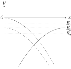
Figure 1: Qualitative shapes of potentials for FRW in the Cases (iii)[small dashed line], (iv)[solid line] and (v)[large dashed line] of Table 1.

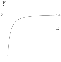
(a) Case (i)

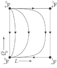
(b) Case (i). Phase portrait.

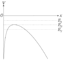
(c) Case (ii)

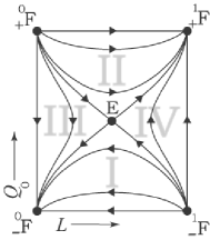
(d) Case (ii). Phase portrait.

Figure 2: Qualitative shapes of potentials for FRW Cases (i) and (ii) in Table 1, with associated flows of the FRW dynamical system (17).

Figs. 1, 2(a), and 2(c) provide a good qualitative understanding of the FRW dynamics, described in Table 1, however, the exact asymptotic behavior of solutions for $x\rightarrow 0,\infty$ depends on the asymptotic properties of the potential. Asymptotically linear equations of state constitute simple examples, since $w\rightarrow w_{0}$ for $x\rightarrow 0$ and $w\rightarrow w_{1}$ for $x\rightarrow\infty$. Consider, e.g., a source that consists of non-interacting perfect fluids with linear equations of state; then $V(x)=-\tilde{\rho}x^{2}=-\sum_{i}\tilde{\rho}_{i0}x^{-(1+3w_{i})}$, where $\tilde{\rho}_{i0}:={\rho}_{i0}/{\rho}_{0}$ and $\sum_{i}\tilde{\rho}_{i0}=1$, and hence $\lim_{x\rightarrow 0}w=\max w_{i}$ and $\lim_{x\rightarrow\infty}w=\min w_{i}$.

3.2 The dynamical system approach

In the dynamical systems picture the FRW models are represented by solutions of the system (5) on a particular invariant manifold obtained by setting $Q_{+}=0$ and $Q_{+}^{\prime}=0$, which implies that $M_{1}=\frac{1}{4}(1-Q_{0}^{2})$ ($4M_{1}^{\prime}=(1-Q_{0}^{2})^{\prime}$ follows). On the FRW subset the general system reduces to

$$\begin{array}[]{lll}Q_{0}^{\prime}&=&-{\textstyle{\frac{1}{8}}}(1-Q_{0}^{2})(3+Q_{0}^{2})(1+3w(L))\,,\\[3.01385pt] L^{\prime}&=&f(L)L(1-L)Q_{0}\,.\end{array}$$ (17)

The conserved energy integral (9) reads

$${\mathcal{E}}(Q_{0},L)=\frac{3(1-Q_{0}^{2})}{3+Q_{0}^{2}}\,V(L)=E<0\>,$$ (18)

cf. also (16). The conserved quantity determines the orbits of (17) in the FRW state space $\{(Q_{0},L)\}$. To simplify the subsequent discussion, we assume an asymptotically linear equation of state that also strictly satisfies asymptotic causality, i.e., $w_{0},w_{1}<1$.

Case (i), i.e., $w>-1/3$ everywhere and asymptotically (strong energy condition), cf. Table 1, yields Fig. 2(a) in the potential approach, while in the dynamical systems approach we obtain the flow depicted in Fig. 2(b). It is easy to see that the models initially expand, reach a point of maximum expansion when $Q_{0}=0$, and then recollapse.

For Case (ii), i.e., matter domination in the limit $L\rightarrow 0$, ($-\frac{1}{3}<w_{0}<1$) and dark energy domination in the limit $L\rightarrow 1$ ($-1\leq w_{1}<-\frac{1}{3}$), the potential has the form depicted in Fig. 2(c). The associated phase portrait in the dynamical systems approach is given in Fig. 2(d); the structure of the phase space is as follows:

1. The energy $E_{S}=V_{max}$, where $V_{max}$ is the maximum of the potential, yields the fixed point E and the four heteroclinic separatrix orbits, which originate from the fixed points ${{}^{1}_{+}}\text{F}$, ${{}^{0}_{-}}\text{F}$ (or E), and end at E (or ${{}^{0}_{-}}\text{F}$, ${{}^{1}_{+}}\text{F}$). The point E represents Einstein’s static universe; its position is $(0,{\mathcal{L}})$ where ${\mathcal{L}}$ is determined by $w({\mathcal{L}})=-1/3$; ${{}^{0,1}_{\pm}}\text{F}$ represent flat fluid FRW models with linear equation of state (when $w_{1}=-1$, ${{}^{1}_{\pm}}\text{F}$ reduce to the de Sitter model). The separatrix orbits divide the phase space into four regions that contain models with distinct qualitative behavior.

2. $E=E_{1}>V_{max}$ yields regions I and II; region I (II) contains forever contracting (expanding) models.

3. $E=E_{2}<V_{max}$ yields regions III and IV. The orbits in region III (IV) represent models that initially expand (contract), reach a point of maximal (minimal) extension at $Q_{0}=0$, and then contract (expand).

The equations in (5) and (17) are completely regular, this is in stark contrast to the non-regularity of the equations used in [7, 8, 9]. Non-regularity leads to a misleading picture, e.g., compare Fig. 2(d) with Fig.1 in [9], where the whole $L=0$ subset has been crushed to a point, which in turn leads to a deformation of the interior orbit structure; moreover, in contrast to $L=0$ in our approach, that point is not part of the state space in [9], since the non-regularized equations blow up there.

Of the cases not discussed above, Case (iii) is closely related to Case (i); in Cases (iv) and (v) the Einstein point lies on the boundaries $L=0$ and $L=1$ respectively; although these cases can also be treated easily, we refrain from doing so here.

Thus both the potential and the dynamical systems approaches provide comprehensive information about the qualititative structure of the FRW solution space, however, in contrast to the potential approach the dynamical systems approach can be applied to more general problems.

4 LRS type IX cosmologies

The foundation of our analysis of the LRS type IX models is the regular dynamical system (5), supplemented by the conserved energy (9). For simplicity we assume $w<1$ and, initially, an asymptotically linear equation of state. We focus on Case (i), where $-1/3<w_{0},w_{1}<1$, and Case (ii), where $-1/3<w_{0}<1$ and $-1\leq w_{1}<-1/3$.

We begin with a local dynamical systems analysis: the fixed points and the associated eigenvalues are given in Table 2. All fixed points correspond to either vacuum solutions or solutions that can be interpreted as perfect fluid solutions with a linear equation of state: F represents flat FRW solutions for a fluid with a linear equation of state; Q stands for the LRS Kasner solution and T for the Taub representation of Minkowski spacetime (see [1]); CS stands for the Bianchi type II Collins and Stewart solution; X stands for a solution discussed, e.g., in [3]; finally E represents Einstein’s static universe. The upper left index refers to $L=0$ or $L=1$; the lower left index refers to $Q_{0}=+1$ or $Q_{0}=-1$, except for _±X where $\pm$ indicates the signs in the expressions for $Q_{0}$ and $Q_{+}$; the lower right index refers to $Q_{+}=+1$ or $Q_{+}=-1$. Note that the fixed points E and _±X do not exist in Case (i) while ${{}^{1}_{\pm}}$CS do not exist in Case (ii). Table 2 shows that in Case (i) all fixed points are saddles except for the source ${}_{+}^{0}\text{T}_{-}$ and the sink ${}_{-}^{0}\text{T}_{+}$. In Case (ii) all fixed points are saddles except for ${}_{+}^{0}\text{T}_{-}$ and ${}_{-}^{1}\text{F}$, which are sources, and ${}_{-}^{0}\text{T}_{+}$ and ${}_{+}^{1}\text{F}$, which are sinks.

F.P	$Q_{0}$	$Q_{+}$	$M_{1}$	$L$	$\lambda_{1}$, $\lambda_{2}$, $\lambda_{3}$, $\lambda_{4}$
${{}^{A}_{\pm}}$F	$\pm 1$	0	$0$	A	$\pm(1+3w_{A})$, $\pm(1+3w_{A})$, $\mp\frac{3}{2}(1-w_{A})$, $\pm S(A)f_{A}$
${{}^{A}_{\pm}}$Q±	$\pm 1$	$\pm 1$	0	A	$\pm 3(1-w_{A})$, $\pm$2, $\mp$4, $\pm S(A)f_{A}$
${{}^{A}_{\pm}}$T∓	$\pm 1$	$\mp 1$	0	A	$\pm 3(1-w_{A})$, $\pm$6, $\pm$12, $\pm S(A)f_{A}$
${{}^{A}_{\pm}}$CS	$\pm 1$	$\pm\frac{(1+3w_{A})}{8}$	$\mathcal{W}_{A}$	A	$\pm\frac{3}{4}(1+3w_{A})$, $\mp\frac{6(1-w_{A})}{8}\left(1\pm i\sqrt{c}\right)$, $\pm S(A)f_{A}$
±X	$\pm\frac{2}{(1-3w_{1})}$	$\,\pm\frac{(1+3w_{1})}{(1-3w_{1})}$	0	1	$\mp\frac{6(1+3w_{1})}{1-3w_{1}}$, $\mp\frac{3}{2}\frac{1-w_{1}}{1-3w_{1}}\left(1\pm\sqrt{d}\right)$, $\mp\frac{2f_{1}}{1-3w_{1}}$
E	0	0	$\frac{1}{4}$	${\mathcal{L}}$	$\frac{3}{4}\sqrt{b}$, $-\frac{3}{4}\sqrt{b}$, $i\sqrt{6}$, $-i\sqrt{6}$

Table 2: Fixed points of the dynamical system (5) and eigenvalues of the linearizations. Here $A$ takes the values $0$ or $1$; $\mathcal{W}_{A}:=3(1-w_{A})(1+3w_{A})/8^{2}$; ${\mathcal{L}}$ is defined by $w({\mathcal{L}}):=-1/3$; $S(0)=1$, $S(1)=-1$, $b:=-2w^{\prime}f({\mathcal{L}}){\mathcal{L}}(1-{\mathcal{L}})$, $c:=(-3w_{A}^{2}+16w_{A}+3)/(2(1-w_{A}))$ and $d:=(24w_{1}^{2}+7w_{1}+1)/(1-w_{1})$; $f({\mathcal{L}})>0$ and $-w^{\prime}=-dw/dL|_{{\mathcal{L}}}>0$, which follows from $d\lambda/dx>0$ and $dw/dx|_{{\mathcal{L}}}<0$.

4.1 The $\mathbf{w=const}$ case

In the case of LRS type IX models with a linear equation of state $w\equiv const$, the equation for $L$ decouples from (5); therefore it suffices to consider the state space $\{(Q_{0},Q_{+},M_{1})\}$. We distinguish two ranges for $w$ that generate different sets of fixed points: $-1/3<w<1$ and $-1\leq w<-1/3$ (we refrain from giving the special case $w=-1/3$). Note that the equation system (and thus the solution structure) for $-1/3<w<1$ coincides with the system on the subsets $L=0$ and $L=1$ in Case (i) and the subset $L=0$ in Case (ii); $-1\leq w<-1/3$ is identical to the $L=1$ subset in Case (ii). The state spaces, and some orbits, are given in Fig. 3.

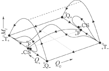
(a) $-1/3<w=const<1$

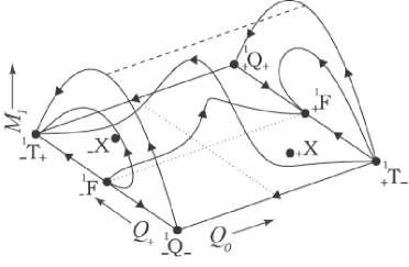
(b) $-1\leq w=const<-1/3$

Figure 3: Typical phase portraits for $-1/3<w\equiv const<1$ and $-1\leq w\equiv const<-1/3$.

4.2 LRS type IX models with $\mathbf{-\frac{1}{3}<w<1}$

Next we consider Case (i), i.e., models with $-1/3<w<1$ and $-1/3<w_{0},w_{1}<1$. We prove that all such models expand from a singularity, reach a point of maximum expansion, and subsequently recollapse to a singularity. Hereby the $\omega$-limit ($\alpha$-limit) of every orbit is located on the 2-plane $(L=0)\cap(Q_{0}=-1)$ ($(L=0)\cap(Q_{0}=+1)$).

The subcase $0<w<1$ is covered by the general results of [5] and [6], where it is proved, for the general Bianchi type IX case, that models do not expand forever, instead they re-collapse to a singularity where certain curvature invariants and the density diverge. Our dynamical systems approach yields more details about the asymptotic dynamics and the methods of our proof are entirely different from those in [5, 6]: our starting point is the dynamical system (5).

On the hypersurface $Q_{0}=0$ we obtain $F>0$ and therefore $Q_{0}^{\prime}<0$; hence, $Q_{0}=0$ acts as a “semipermeable membrane” for the flow of the system (5). The hypersurface cuts the interior state space in two halves, a future invariant half $Q_{0}<0$, where $L$ monotonically decreases, i.e., $L^{\prime}<0$, and a past invariant half $Q_{0}>0$, where $L^{\prime}>0$. It follows that fixed points and periodic orbits are excluded in the interior of the state space.

Application of the principle of monotone functions, see, e.g., [1], and investigation of the structure of the flow on $Q_{0}=0$, yields that the $\omega$-limit of the future invariant set $Q_{0}<0$ must be contained in $L=0$; analogously the $\alpha$-limit of every orbit in $Q_{0}>0$ must lie on $L=0$. More specifically, the $\omega$-limit is located on the 2-plane $(L=0)\cap(Q_{0}=-1)$. To show this, consider an orbit $(Q_{0},Q_{+},M_{1},L)(\tau)$ in $Q_{0}<0$. Since $L\rightarrow 0$ for $\tau\rightarrow\infty$, the function $V$, cf. Fig. 2(a), satisfies $V\rightarrow-\infty$. The integral of motion (9) fulfills

$$(1-Q_{0}^{2})^{4/3}=\frac{4^{4/3}\,\Omega_{D}\,M_{1}^{1/3}\,E}{3\,V}\>\rightarrow\>0\qquad(\tau\rightarrow\infty)\>,$$ (19)

and thus $Q_{0}\rightarrow-1$ ($\tau\rightarrow\infty$), as claimed; analogously, the $\alpha$-limit of $Q_{0}>0$ lies on $(L=0)\cap(Q_{0}=+1)$.

As regards the future asymptotic behavior of orbits in $Q_{0}>0$ (and the $\alpha$-limit of $Q_{0}<0$), there exist, a priori, two possibilities: an orbit either passes through $Q_{0}=0$ into $Q_{0}<0$, and thus converges to $(L=0)\cap(Q_{0}=-1)$, or it remains in $Q_{0}>0$ for all times. However, a proof by contradiction shows that the second scenario is excluded: let us assume that the solution satisfies $Q_{0}>0\>\forall\,\tau$. The monotonicity principle then implies $L\rightarrow 1$ for $\tau\rightarrow\infty$. Hence, $V\rightarrow 0$ and, from (9),

$$\Omega_{D}M_{1}^{1/3}=\frac{3\,(1-Q_{0}^{2})^{4/3}\,V}{4^{4/3}\,E}\>\rightarrow\>0\qquad(\tau\rightarrow\infty)\>.$$ (20)

It follows that either $\Omega_{D}\rightarrow 0$ or $M_{1}\rightarrow 0$ as $\tau\rightarrow\infty$. This restricts the $\omega$-limit of the orbit to the 2-surface

$$\left[(L=1)\cap(Q_{0}\geq 0)\cap(\Omega_{D}=0)\right]\>\,\cup\left[(L=1)\cap(Q_{0}\geq 0)\cap(M_{1}=0)\right]\>.$$ (21)

Since the $\omega$-limit set of the orbit is located on a 2-surface, the $\omega$-limit is either a fixed point, a periodic orbit, a heteroclinic cycle, or it is the whole 2-surface that acts as the attractor. The local analysis of ${}^{1}_{+}\text{Q}_{+}$, ${}^{1}_{+}\text{T}_{-}$, and ${}^{1}_{+}\text{F}$ reveals that these fixed points are saddles such that no orbit from the interior of the state space can be attracted. Moreover, the surface (21) does neither contain periodic orbits nor heteroclinic cycles; the possibility that the $\omega$-limit of the orbit is the whole 2-surface is excluded by the structure of the flow as well. Since the 2-surface (21) does not act as an $\omega$-limit set, we have arrived at a contradiction; $Q_{0}>0\>\forall\,\tau$ is thus excluded and therefore the $\omega$-limit of an orbit in $Q_{0}>0$ lies on $(L=0)\cap(Q_{0}=-1)$.

Note that the “saddle structure” of the surface (21) is valid for any value $w_{1}>-1/3$; it follows that it is not necessary to assume asymptotic linearity of the equation of state, i.e., $w\rightarrow w_{1}>-1/3$ is not required, $(\inf w)>-1/3$ is a sufficient assumption.

4.3 LRS type IX models with $\mathbf{-1<w<1}$

Consider now Case (ii), i.e., models with $-1/3<w<1$ for $L<{\mathcal{L}}$, $w({\mathcal{L}})=-1/3$, $-1\leq w<-1/3$ for $L>{\mathcal{L}}$, and $w^{\prime}:=dw/dL\,|_{{\mathcal{L}}}<0$, whereby $V$ has a single maximum, cf. Sec. 3.1.

Below we give a comprehensive description of the dynamics of models in a neighborhood of the Einstein point and of the asymptotic behavior of these models. The analogous problem has been investigated in [7, 8] for the special case of a fluid with a linear equation of state and a cosmological constant, however, we arrive at different conclusions. We demonstrate that the asymptotic behavior of models close to the Einstein point is predictable and not governed by “homoclinic phenomena and chaos”. In addition we also show several global results.

Our analysis is based on our dynamical systems formulation, i.e., the regular system (5) on the compact state space ${}^{4}\textbf{X}$; the analysis rests on three cornerstones: the local dynamical systems analysis of the Einstein point E, in particular center manifold reduction; the use of the conserved quantity ${\mathcal{E}}$; the recognition and use of the close relationship between the dynamics of the full system and the FRW subset.

The first cornerstone in our analysis is the local dynamical systems analysis of the Einstein point E. Two eigenvalues, $\lambda_{1,2}=\pm 3\sqrt{b}/4$, are associated with eigenvectors that lie in the FRW plane, $\mathbf{v}_{1,2}=(1,0,0,\pm 2\sqrt{b}/(3w^{\prime}))$, where $b:=-2w^{\prime}f({\mathcal{L}}){\mathcal{L}}(1-{\mathcal{L}})$; two purely imaginary eigenvalues, $\lambda_{3,4}=\pm i\sqrt{6}$, lead to a rotation in the plane orthogonal to the FRW plane. Hence the linear space at E decomposes into the direct sum $E^{s}\oplus E^{u}\oplus E^{c}$ of a one-dimensional stable (unstable) subspace $E^{s}$ ($E^{u}$), and a two-dimensional center subspace $E^{c}=\langle(0,1,0,0),(0,0,1,0)\rangle$.

To adapt to E and the structure $E^{s}\oplus E^{u}\oplus E^{c}$ we introduce new variables,

$$\tilde{q}_{0}=\frac{1}{2}\left(Q_{0}+\frac{9\,w^{\prime}}{8\,\lambda_{1}}\>(L-{\mathcal{L}})\,\right)\,,\>\>q_{+}=Q_{+}\,,m_{1}=M_{1}-\frac{1}{4}\,,\>\>\tilde{l}=\frac{1}{2}\left(Q_{0}-\frac{9\,w^{\prime}}{8\,\lambda_{1}}\>(L-{\mathcal{L}})\,\right)\,,$$ (22)

which transform the dynamical system (5) to

$$\begin{pmatrix}\tilde{q}_{0}^{\prime}\\ \tilde{l}^{\prime}\end{pmatrix}=\begin{pmatrix}\lambda_{1}&0\\ 0&\lambda_{2}\end{pmatrix}\begin{pmatrix}\tilde{q}_{0}\\ \tilde{l}\end{pmatrix}+\begin{pmatrix}N_{{\tilde{q}}_{0}}\\ N_{{\tilde{l}}}\end{pmatrix}\,,\quad\begin{pmatrix}q_{+}^{\prime}\\ m_{1}^{\prime}\end{pmatrix}=\begin{pmatrix}0&4\\ -\frac{3}{2}&0\end{pmatrix}\begin{pmatrix}q_{+}\\ m_{1}\end{pmatrix}+\begin{pmatrix}N_{q_{+}}\\ N_{m_{1}}\end{pmatrix}\,,$$ (23)

where the nonlinear terms are collected in the respective terms $N=N(\tilde{q}_{0},q_{+},m_{1},\tilde{l})$.

The invariant center manifold $M_{E}^{c}$ is two-dimensional, tangential to $E^{c}$, and contains E. Locally it is represented by the graph of a function $h:E^{c}\rightarrow E^{s}\oplus E^{u}$,

$$(q_{+},m_{1})\mapsto(\tilde{q}_{0},\tilde{l})=(h_{q_{0}}(q_{+},m_{1}),h_{l}(q_{+},m_{1}))\,,$$ (24)

which satisfies $h(0)=0$ and $\text{grad}\>h(0)=0$. Center manifold reduction, see, e.g. [15], reduces the full nonlinear system (23) to the locally equivalent system

$$\begin{pmatrix}\tilde{q}_{0}^{\prime}\\ \tilde{l}^{\prime}\end{pmatrix}=\begin{pmatrix}\lambda_{1}&0\\ 0&\lambda_{2}\end{pmatrix}\begin{pmatrix}\tilde{q}_{0}\\ \tilde{l}\end{pmatrix}\>,\quad\begin{pmatrix}q_{+}^{\prime}\\ m_{1}^{\prime}\end{pmatrix}=\begin{pmatrix}0&4\\ -\frac{3}{2}&0\end{pmatrix}\begin{pmatrix}q_{+}\\ m_{1}\end{pmatrix}+\begin{pmatrix}N_{q_{+}}\\ N_{m_{1}}\end{pmatrix}\ ,$$ (25)

where $N=N((h_{q_{0}}(q_{+},m_{1}),q_{+},m_{1},h_{l}(q_{+},m_{1}))$.

In general it is impossible to obtain the graph of $h$ in terms of elementary functions, however, approximate solutions can be obtained by series expansions:

$$h_{q_{0}}(q_{+},m_{1})=\tilde{q}_{0}=\frac{1}{2}\left(q_{0}+\frac{9}{8}\,\frac{w^{\prime}}{\lambda_{1}}\,l\,\right)\,,\quad h_{l}(q_{+},m_{1})=\tilde{l}=\frac{1}{2}\left(q_{0}-\frac{9}{8}\,\frac{w^{\prime}}{\lambda_{1}}\,l\,\right)\>,$$ (26)

where

$$q_{0}=-2^{4}w^{\prime}\,k\,q_{+}m_{1}+O(\|(q_{+},m_{1})\|^{3})\>,\quad l={\textstyle{\frac{3b+2^{6}}{3}}}k\,q_{+}^{2}+{\textstyle{\frac{2^{9}}{3^{2}}}}k\,m_{1}^{2}+O(\|(q_{+},m_{1})\|^{3})\,,$$ (27)

where $k:=-2^{4}/(3w^{\prime}(2^{7}+3b))$, $b:=-2w^{\prime}\,f({\mathcal{L}}){\mathcal{L}}(1-{\mathcal{L}})$.

The coordinates in (25) are not the coordinates (22), but coordinates adapted to the center manifold structure. We assume that the two coordinate systems agree to first order; this is justified since $E^{u}\oplus E^{s}$ coincides with the FRW invariant subset and because of (26) and (27). To avoid excessive notation we use the same symbols for the coordinates of (22) and (25).

The reduced system (25) represents a decoupled system, and hence the properties of the flow in the neighborhood of E can be deduced straightforwardly. The center manifold $M_{E}^{c}$ is represented by $\tilde{q}_{0}=\tilde{l}=0$, and the induced dynamical system by the $(q_{+},m_{1})$-system of (25). The solutions are “circular” periodic orbits centered about the fixed point E, as we prove below. The fixed point E is an $\omega$-limit for two orbits and an $\alpha$-limit for another pair, which follows from setting $q_{+}=m_{1}=0$ and $\tilde{q}_{0}=0$ (or $\tilde{l}=0$); the four orbits are the separatrix orbits in the FRW plane, see Fig. 2(d). Each periodic orbit acts as $\omega$-limit for two one-parameter families of orbits: in the invariant set $\tilde{q}_{0}=0$, Eq. (25) describes one one-parameter family of orbits in the half-space $(\tilde{l}>0)$ (another one in $\tilde{l}<0$) that spiral down (up) towards the periodic orbit at $\tilde{l}=0$; similarly, in the invariant space $\tilde{l}=0$, the periodic orbit is the $\alpha$-limit for another two one-parameter families of spirals. For general initial data $(\tilde{q}_{0}\neq 0,\tilde{l}\neq 0)$ the closed orbits act as a “saddles”, see Fig. 9 below; we thus observe a natural generalization of the FRW picture.

The second cornerstone in our analysis is the conserved quantity ${\mathcal{E}}$. To locate E at the origin we introduce the variables

$$q_{0}=Q_{0}\,,\,\,q_{+}=Q_{+}\,,\,\,m_{1}=M_{1}-1/4\,,\,\,l=L-{\mathcal{L}}\,,$$ (28)

so that Eq. (9) is transformed to

$${\mathcal{E}}(q_{0},q_{+},m_{1},l):=\frac{3\,(1-q_{0}^{2})^{4/3}\,V({\mathcal{L}}+l)}{(3-4q_{+}^{2}-4m_{1})(1+4m_{1})^{1/3}}=E\,.$$ (29)

To discuss the 3-hypersurfaces of constant energy, ${\mathcal{E}}=E$, in a neighborhood of E, we expand (29) up to second order, using $V({\mathcal{L}}+l)=V_{max}+V^{\prime\prime}({\mathcal{L}})l^{2}$ where $V_{max}=V({\mathcal{L}})$ and $V^{\prime\prime}<0$,

$$-4\frac{V_{max}}{E}q_{0}^{2}+\frac{3}{2}\frac{V^{\prime\prime}({\mathcal{L}})}{E}\,l^{2}+\|(q_{+},m_{1})\|^{2}=3\left(1-\frac{V_{max}}{E}\right)\,,$$ (30)

where $\|(q_{+},m_{1})\|^{2}:=4q_{+}^{2}+16m_{1}^{2}/3$.

We employ ${\mathcal{E}}$ to prove that the orbits on the center manifold, i.e., the solutions of the $(q_{+},m_{1})$-system in (25), are periodic. The idea is simple: the intersection of a hypersurface ${\mathcal{E}}=E$ with a transversal surface that is itself invariant under the flow of the dynamical system yields an orbit with energy $E$ on that surface. It is not possible to study $M_{E}^{c}\cap({\mathcal{E}}=E)$ directly, however, the investigation of $E^{c}\cap({\mathcal{E}}=E)$ turns out to be sufficient. We therefore set $q_{0}=l=0$ in (29), and obtain $3-(3-4q_{+}^{2}-4m_{1})(1+4m_{1})^{1/3}=3(1-V_{max}/E)$, which describes a family of closed curves, parametrized by $E$. In an appropriately small neighborhood of the origin, these curves can be approximated by $\|(q_{+},m_{1})\|^{2}=3(1-V_{max}/E)=const$, where $E<V_{max}$, cf. (30) with $q_{0}=l=0$. Since $\text{grad}\,{\mathcal{E}}\sim\big{(}0,c_{1}q_{+},c_{2}(4m_{1}+q_{+}^{2}),0\big{)}$, where $c_{1}$, $c_{2}$ are non-vanishing, it follows that the surface ${\mathcal{E}}=E$ is orthogonal to $E^{c}$ at the intersection; this guarantees the intersection to be a closed curve also when $E^{c}$ is continuously deformed to $M_{E}^{c}$.

Every solution in a sufficiently small neighborhood of E obeys the relation $\|(q_{+},m_{1})\|^{2}=const$ approximately, since the equations for $(q_{+},m_{1})$ decouple and yield $\|(q_{+},m_{1})\|^{2}=const$ in (25). Hence the hypersurface $\|(q_{+},m_{1})\|=const$ is a (locally) invariant set. Each orbit in this invariant set gives rise to a one-parameter family of orbits that differ only w.r.t. the (polar) angle along $\|(q_{+},m_{1})\|=const$. Therefore, one can represent an orbit –modulo its phase– by an orbit in the 3-space ${}^{3}\textbf{X}=\{\,\big{(}q_{0},l,\|(q_{+},m_{1})\|\,\big{)}\,\}$ that fulfills $\|(q_{+},m_{1})\|=const$; hereby the four-dimensional dynamical picture is reduced to a three-dimensional one.

The state space ${}^{3}\textbf{X}$ is endowed with a Lorentzian scalar product of signature ($-$$+$$+$), Eq. (30) describes 2-surfaces of constant Lorentz norm. The light cone, $E=V_{max}$, divides the state space into three disconnected regions: $E>V_{max}$ yields region I, the chronological past of E, and region II, the chronological future; $E<V_{max}$ yields region III/IV, the spacelike region, see Fig. 5. Note that the disconnected regions III and IV of the FRW picture 2(d) are merged to one connected region III/IV. The coordinates $\tilde{q}_{0}$ and $\tilde{l}$ are null coordinates w.r.t. the metric; this can be seen from (22) and the relation $V^{\prime\prime}({\mathcal{L}})=-3w^{\prime}V_{max}\,[f({\mathcal{L}}){\mathcal{L}}(1-{\mathcal{L}})^{-1}]^{-1}$, which can be derived from (11).

The third cornerstone in our analysis is the close connection to the FRW case. In ${}^{3}\textbf{X}$, the FRW plane is given by $\|(q_{+},m_{1})\|=0$. The separatrix orbits, $E=V_{\max}$, are given by the null rays ${\tilde{q}}_{0}=0$ and $\tilde{l}=0$. Let $\tilde{\nu}^{+}_{q}$ ($\tilde{\nu}^{-}_{q}$) denote the future (past) null ray along the ${\tilde{q}}_{0}$-axis, and $\tilde{\nu}^{\pm}_{l}$ the null rays along the $\tilde{l}$-axis, see Fig. 4. From Sec. 3.2 we know the global asymptotics,

$$\begin{split}&\tilde{\nu}^{+}_{q}\leftrightarrow(\text{E}\rightarrow{}^{1}_{+}\text{F})\,,\qquad\tilde{\nu}^{+}_{l}\leftrightarrow({}^{0}_{+}\text{F}\rightarrow\text{E})\,,\\ &\tilde{\nu}^{-}_{q}\leftrightarrow(\text{E}\rightarrow{}^{0}_{-}\text{F})\,,\qquad\tilde{\nu}^{-}_{l}\leftrightarrow({}^{1}_{-}\text{F}\rightarrow\text{E})\>.\end{split}$$ (31)

Orbits close to $\tilde{\nu}^{\pm}_{q,l}$ are dragged along and thus exhibit similar asymptotic behavior as $L\rightarrow 0,1$. However, in the general picture the FRW attractor ${}^{0}_{-}\text{F}$ is generalized to $(L=0)\cap(Q_{0}=-1)$, which describes the contracting Bianchi type II boundary with a linear equation of state characterized by $w_{0}$ (the FRW source ${}^{0}_{+}\text{F}$ is generalized to $(L=0)\cap(Q_{0}=+1)$, which describes the expanding version of the type II boundary); see App. B.1. A priori the FRW source ${}^{1}_{-}\text{F}$ becomes $(L=1)\cap(Q_{0}=-1)$, however, on that surface it is only the fixed point ${}^{1}_{-}\text{F}$ that can act as an $\alpha$-limit; a similar $\omega$-limit statement holds for ${}^{1}_{+}\text{F}$.

A combination of the ideas of our analysis yields an effective description of the dynamics close to E: in ${}^{3}\textbf{X}$, an orbit with a given energy $E$ lies on a hyperboloid (or light cone) of constant Lorentz norm, cf. (30); simultaneously, every orbit satisfies $\|(q_{+},m_{1})\|=const$. Therefore, the intersections of the energy-hyperboloids with the planes $\|(q_{+},m_{1})\|=const$ yield a complete description of all orbits in ${}^{3}\textbf{X}$; furthermore, the asymptotics of (31) and the above generalization determines the asymptotics of the orbits. We investigate the scenarios case by case:

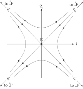
Figure 4: The FRW plane $\|(q_{+},m_{1})\|=0$ in the space ${}^{3}\textbf{X}$. Four null rays, $\nu^{\pm}_{q,l}$, converge to the Einstein point E as $\tau\rightarrow\pm\infty$.

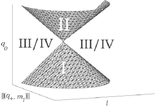
Figure 5: The light cone $E=V_{max}$ in ${}^{3}\textbf{X}$ divides the state space in three regions that generalize the regions in the FRW picture 2(d).

When $E>V_{max}$, Eq. (30) describes two “mass” hyperboloids in ${}^{3}\textbf{X}$; one in region I and one in region II, see Fig. 6. Intersection with planes $\|(q_{+},m_{1})\|=const$ yields a family of spacelike hyperbolas which are parallel to null rays asymptotically, Fig. 6; this indicates that the hyperbolas of region I originate from ${}^{1}_{-}\text{F}$, as $\tilde{\nu}^{-}_{l}$ does, and end on $(L=0)\cap(Q_{0}=-1)$ like $\tilde{\nu}^{-}_{q}$. Analogously, the hyperbolas in region II originate from $(L=0)\cap(Q_{0}=+1)$ and end at ${}^{1}_{+}\text{F}$. The described global asymptotic behavior of orbits also remains true for orbits remote from E, as proved in App. B. Thus the FRW picture is generalized: region I (II) contains models that contract (expand) forever.

When $E=V_{max}$, Eq. (30) describes the light cone in ${}^{3}\textbf{X}$, see Fig. 5. Intersection with the FRW plane $\|(q_{+},m_{1})\|=0$ yields the four null rays discussed above, cf. (31) and Fig. 4. Intersection with planes $\|(q_{+},m_{1})\|=const>0$ yields a family of hyperbolas that resemble those in the $E>V_{max}$ case; the global behavior is thus analogous.

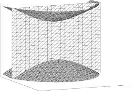
Figure 6: Case $E>V_{max}$. Intersection of the mass hyperboloids of energy $E$ with a plane $\|(q_{+},m_{1})\|=const$ in ${}^{3}\textbf{X}$ yields two hyperbolas, one in region I and one in region II. The axes are the same as in Fig. (5).

Finally, when $E<V_{max}$, Eq. (30) describes one hyperboloid of positive Lorentz norm in the region III/IV in ${}^{3}\textbf{X}$. We distinguish three subcases:

Case (a): Intersection with planes $\|(q_{+},m_{1})\|=const<3(1-\frac{V_{max}}{{E}})$ yields a family of timelike hyperbolas, see Fig. 8(a). This leads to a generalization of the behavior of orbits in region III and IV in FRW: we distinguish models that originate from ${}^{1}_{-}\text{F}$ (resp. $(L=0)\cap(Q_{0}=+1)$) and end in ${}^{1}_{+}\text{F}$ ($(L=0)\cap(Q_{0}=-1)$).

Case (b): Intersection with a plane $\|(q_{+},m_{1})\|=3(1-\frac{V_{max}}{{E}})$ yields the point $\|(q_{+},m_{1})\|=3(1-\frac{V_{max}}{{E}})$, $q_{0}=0$, $l=0$, which represents a periodic orbit, and four in/outgoing null rays (cf. also the discussion following Eq. (30)), see Fig. 8(b). Two of these null rays represent orbits that originate from either $(L=0)\cap(Q_{0}=+1)$ or ${}^{1}_{-}\text{F}$ and converge to the periodic orbit as $\tau\rightarrow\infty$; the other two originate from the center manifold orbit and end at either $(L=0)\cap(Q_{0}=-1)$ or ${}^{1}_{+}\text{F}$. The FRW picture is thus generalized; periodic center manifold orbits (one for each value of $E$) take the place of the Einstein point E, see Fig. 7. This figure also indicates how the abstract ${}^{3}\textbf{X}$ picture is related to the ${}^{4}\textbf{X}$ state space picture, cf. Fig. 8(a) and Fig. 7.

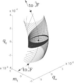
(a) Spiral tubes that describe the stable manifold of a periodic orbit; on each side of the periodic orbit 25 spiral orbits are depicted.

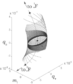
(b) Spiral tubes that describe the unstable manifold of a periodic orbit; each side of the periodic orbit consists of 25 spiral orbits.

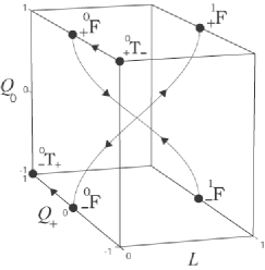
(c) The four spiral tubes of Figs. (a) and (b) in the state space; the diameter of the tubes is too small to be resolved. Note that in the projection of Figs. (a) and (b) the tubes would have overlapped.

Figure 7: Illustration of the close relationship between the dynamics close to E and FRW dynamics. At the scale of Fig. (c) there is no visible difference between this figure and the analogous figure depicting the FRW separatrices in the same projection, except that the orbits do not converge to ${}^{0}_{\pm}\text{F}$ in general, but to the generic limits ${}^{0}_{\mp}\text{T}_{\pm}$, cf. App. B.1 and Fig. 10. In this figure the matter content is radiation and a cosmological constant, however, the qualitative behavior is the same for any matter source that admits the Einstein static solution.

Case (c): Intersection with planes $\|(q_{+},m_{1})\|=const>3(1-\frac{V_{max}}{{E}})$ results in a family of spacelike hyperbolas, see Fig. 8(c); this case resembles the $E>V_{max}$ case and yields similar behavior. Accordingly, there exist models that expand forever from a singularity to infinite dispersion, despite that their energy $E$ is lower than the “potential barrier” $V_{max}$. In this case $\|(q_{+},m_{1})\|$ acts as an additional energy that is sufficiently large to lift the orbit over the top of the hill from the “side of recollapse” to the “side of expansion” in Fig. 2(c), when it passes through the neighborhood of E.

When $E$ is sufficiently close to $V_{max}$, and if the orbit passes through a sufficiently small neighborhood of E, the presented arguments about global asymptotic behavior are mathematically rigorous. The known asymptotics of the null ray orbits (31), and continuous dependence on initial data, guarantees that orbits that are close to the null rays are dragged to neighborhoods of ${}^{0,1}_{\pm}\text{F}$. The fixed point ${}^{1}_{+}\text{F}$ is a sink, hence all orbits that pass through a sufficiently small neighborhood of ${}^{1}_{+}\text{F}$ end in ${}^{1}_{+}\text{F}$. An analogous statement holds for the source ${}^{1}_{-}\text{F}$. When an orbit is dragged along $\tilde{\nu}_{q}^{-}$ towards ${}^{0}_{-}\text{F}$, it represents a model that contracts when $L<{\mathcal{L}}$; in App. B we show that it must continue to contract and reach $(L=0)\cap(Q_{0}=-1)$. Analogously, orbits that head for ${}^{0}_{+}\text{F}$ along $\tilde{\nu}_{l}^{+}$ (for $\tau\rightarrow-\infty$) expand forever from $(L=0)\cap(Q_{0}=1)$.

(a) $\|(q_{+},m_{1})\|<3(1-\frac{V_{max}}{{E}})$

(b) $\|(q_{+},m_{1})\|=3(1-\frac{V_{max}}{{E}})$

(c) $\|(q_{+},m_{1})\|>3(1-\frac{V_{max}}{{E}})$

Figure 8: Case $E<V_{max}$. Intersection of the timelike hyperboloids with energy $E$ with different planes $\|(q_{+},m_{1})\|=const$. We obtain timelike hyperbolas in Case (a), a vertex and a null cone in Case (b), and spacelike hyperbolas in (c). The vertex of the null cone in (b) represents a closed orbit in the center manifold. The global asymptotic behavior of the orbits is governed by the null ray orbits $\tilde{\nu}^{\pm}_{l,q}$, cf. Fig. 4. The axes in the figures are the same as in Fig. (5).

We emphasize that the dynamics of the LRS type IX models is closely related to the FRW case and completely predictable near the Einstein point E as regards asymptotic states: in the FRW case, the asymptotic states are determined by the energy $E$; in the LRS type IX case, the asymptotic states are determined by the energy $E$ and by the value of $\|(q_{+},m_{1})\|=const$. This disproves the claims of [7, 8] about non-predicability of asymptotic states for models close to E. Moreover, as shown in Appendix B, the homoclinic behavior of orbits asserted in [7, 8], can be disproved not only for orbits that pass through a neighborhood of E, but also for large regions of the state space, such as $L\leq{\mathcal{L}}$, $L>\tilde{{\mathcal{L}}}_{E}$: in these regions the asserted orbits whose $\alpha$- and $\omega$-limit is the same periodic orbit cannot exist. Furthermore, numerical results reveal that the qualitative features described above for a sufficiently small neighborhood of E carry over to a large neighborhood of E and a large range of energies, as can be seen in Fig. 9 and Fig. 10. This indicates that the assertions about “homoclinic phenomena and chaos” are wrong for the entire state space.

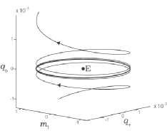
(a) Periodic orbits act as “saddle” orbits in the neighborhood of E.

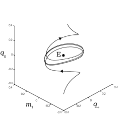
(b) The center manifold dominates even far away from E.

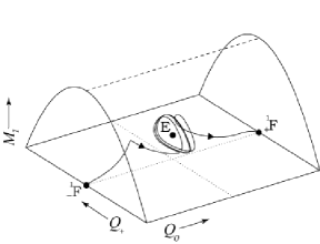
(c) The same orbit as in (b), now depicted in the state space through a $(Q_{0},Q_{+},M_{1})$-projection.

Figure 9: Example of the effect of the center manifold on dynamics. The source is orthogonal dust and a positive cosmological constant, however, the pictures depict behavior that is typical for all sources that admit a unique Einstein point E.

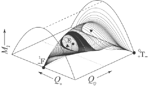
(a) Spiral tubes that emanate from a periodic orbit far from the Einstein point. On each side of the periodic orbit, 25 orbits with the same energy that describe the stable manifold of the periodic orbit, are depicted.

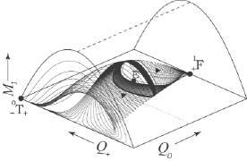
(b) Spiral tubes that emanate from a periodic orbit far from the Einstein point. On each side of the periodic orbit, 25 orbits with the same energy that describe the unstable manifold of the periodic orbit, are depicted.

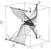
(c) The four spiral tubes of Figs. (a) and (b) in the state space; they emanate from the stable Friedmann/Taub points on the expanding and contracting Bianchi type II boundary subsets.

Figure 10: Illustration of the dynamics far from the Einstein point: the qualitative structure of the flow is still the one of a small neighborhood of E. Clearly there is no “homoclinic chaos.” In this figure the matter content is radiation and a cosmological constant, however, the qualitative behavior is the same for any matter source that admits the Einstein static solution.

Finally note that the discussion of the dynamics in the neighborhood of the Einstein point E is independent of the assumption of asymptotic linearity of the equation of state and that the global asymptotic behavior of orbits remains valid in a wide sense. The boundaries are no longer part of the systems, however, it is still correct to state that the $\alpha$- and $\omega$-limits of orbits are located on $(L=0)\cap(Q_{0}=\pm 1)$ and $(L=1)\cap(Q_{0}=\pm 1)$.

5 Kantowski-Sachs cosmologies

The coupled system of equations for the Kantowski-Sachs models is obtained from the general system (5) by setting $M_{1}=0$; we thus have the three-dimensional state space $\{(Q_{0},Q_{+},L)\}$ depicted in Fig. 11. The coupled system admits a number of equilibrium points whose associated eigenvalues are given in Table 3.

F.P	$\lambda_{1}$	$\lambda_{2}$	$\lambda_{3}$
${}^{A}_{\pm}$F	$\pm(1+3w_{A})$	$\mp\frac{3}{2}(1-w_{A})$	$\pm S(A)f_{A}$
${{}^{A}_{\pm}}$Q±	$\pm$2	$\pm 3(1-w_{A})$	$\pm S(A)f_{A}$
${{}^{A}_{\pm}}$T∓	$\pm 6$	$\pm 3(1-w_{A})$	$\pm S(A)f_{A}$
±X	$\mp\frac{2f_{1}}{1-3w_{1}}$	$\mp\frac{3}{2}\frac{1-w_{1}}{1-3w_{1}}\left(1+\sqrt{d}\right)$	$\mp\frac{3}{2}\frac{1-w_{1}}{1-3w_{1}}\left(1-\sqrt{d}\right)$

Table 3: Fixed points and eigenvalues for the Kantowski-Sachs submanifold. Here $A=0,1$, $S(0)=1$, $S(1)=-1$, $d=(24w_{1}^{2}+7w_{1}+1)/(1-w_{1})$.

It follows that in Case (i) all fixed points are saddles except for ${}_{+}^{0}\text{T}_{-}$, which is a source, and ${}_{-}^{0}\text{T}_{+}$, which is a sink. In Case (ii) all fixed points are saddles except for ${}_{+}^{0}\text{T}_{-}$ and ${}_{-}^{1}\text{F}$, which are sources, and ${}_{-}^{0}\text{T}_{+}$ and ${}_{+}^{1}\text{F}$, which are sinks.

In Case (i) all models expand from a singularity, reach a point of maximum expansion, and then recollapse to a singularity, as follows from an analysis similar to that of the LRS type IX case. The situation in Case (ii) is more complicated; local analysis limits the possibilities somewhat but numerics is required to give a detailed picture. Fig. 11 illustrates various possibilities, e.g., there are solutions that expand from singularities to infinitely dispersed isotropic states and solutions that contract from infinitely dispersed isotropic states to singularities.

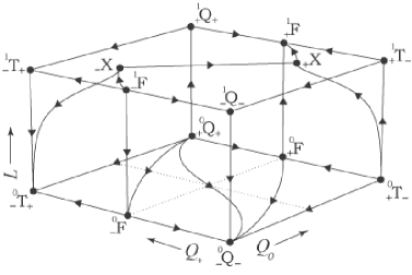
Figure 11: The Kantowski-Sachs submanifold. Case (ii).

6 Conclusion and outlook

In this paper we have regularized Einstein’s field equations and obtained a dynamical system on a compact state space for the LRS Bianchi type IX and Kantowski-Sachs perfect fluid models with a barotropic equation of state. This allowed us to systematically study the effects of matter properties on cosmological evolution, and we obtained a global picture of the dynamical possibilities. In type IX, the cornerstones of our analysis were: center manifold theory in connection with Einstein’s static solution –when existent; an “energy integral” that severely restricted the dynamics; a close connection between the FRW and LRS type IX cases. This led to a comprehensive description of the dynamics in the neighborhood of Einstein’s static model: given an initial value in the state space in the neighborhood of Einstein’s model, it is possible to predict whether the solution will expand to an infinite dilute final state or eventually contract to a singularity. This disproves previous assertions that the dynamics near the Einstein model exhibits non-predictability and chaos. The present formalism is generalizable to cover more general models such as general Bianchi type IX models for which it is also possible to derive a conserved energy which, together with center manifold theory, again severely restrict the dynamics; indeed, we expect that the conclusions drawn in this paper will have direct bearing on this problem as well. In addition to this we have obtained several global results; again we expect our methods and results to be generalizable to the general Bianchi type IX case.

The present approach is also of relevance for the forever expanding Bianchi type I–VIII perfect fluid models. As in the present case one can introduce a variable $L$ and obtain an autonomous formulation, however, in this case one can also use $\ln(\ell/\ell_{0})$ as a time variable (the natural time variable when $H$ is used as the normalization factor, as discussed in [1]), which then leads to that $w$ becomes a time dependent function and thus that one obtains a non-autonomous problem. However, in the case of an asymptotic linear equation of state one obtains an asymptotically autonomous problem and for certain problems one can then apply the Strauss-Yorke theorem to determine the asymptotic dynamics [16], [17]. Both approaches are expected to have advantages and disadvantages that depend on the problem at hand. Although one can draw the conclusion that Bianchi type I–VIII perfect fluid models with $\rho>0$ are forever expanding, the details of how this actually happens is a quite intricate problem due to asymptotic self-similarity breaking, which occur for the more general classes of models [18], [17]; we expect asymptotic self-similarity breaking to hold for the same class of models also for asymptotically linear equations of state, but the details will depend on the equation of state.

We thus expect that some of the ideas in this paper are generalizable to other SH models, however, we also believe that some ideas are generalizable to models with fewer symmetries, even to models with no symmetries at all, so-called $G_{0}$ models, particularly when it comes to asymptotic dynamics associated with singularity formation. Again one can treat a barotropic equation of state by introducing a function similar to $L$ that parametrize the equation of state suitably. In special cases of matter dominated singularities additional assumptions like asymptotic linearity will have to be imposed on the equation of state, however, generically the singularity is expected to be “vacuum dominated” [10]; in this case we expect that one can treat equations of state with quite general asymptotic behavior.

Acknowledgements

We would like to thank Alan Rendall for comments on an earlier draft. C.U. was in part supported by the Swedish Research Council.

Appendix A Dynamical systems nomenclature and definitions

Consider a dynamical system $\dot{y}=f(y)$ and the associated flow $\Phi_{t}$. The $\omega$-limit $\omega(x)$ ($\alpha$-limit $\alpha(x)$) of a point $x$ is defined as the set of all accumulation points of the future orbit $\{\Phi_{t}(x)\,|\,t>0\}$ (past orbit $\{\Phi_{t}(x)\,|\,t<0\}$) of $x$. The $\omega$-limit of a set $S$ is $\omega(S)=\bigcup_{x\in S}\omega(x)$. An orbit $\{\Phi_{t}(x)\,|\,t\in\mathbb{R}\}$ is called homoclinic, if there exists a (fixed) point $z$ such that $\alpha(x)=\omega(x)=\{z\}$; an orbit is called heteroclinic if it originates from a fixed point $z_{1}$ and ends in a different fixed point $z_{2}$. A set $S$ is called future (past) invariant, if $\Phi_{t}(S)\subseteq S\>\forall\,t>0$ ($\forall\,t<0$).

The monotonicity principle states that if there is a function $Z$ on an invariant set $S$ that is strictly decreasing along orbits, then $\omega(S)=\{s\in\bar{S}\backslash S\,|\,\lim_{x\rightarrow s}Z(x)\neq\sup_{S}Z\}$, and analogously for the $\alpha$-limit.

Two dynamical systems are called (locally) equivalent, if there exists a homeomorphism (of coordinates) $\Psi$ such that the flows are topologically equivalent $\Phi_{t}^{1}=\Psi^{-1}\circ\Phi_{t}^{2}\circ\Psi$. Under certain conditions the equivalence is a diffeomorphism.

Appendix B Asymptotic states and global dynamics

In this section we discuss aspects of the global dynamics of case (ii) of the LRS type IX models: first we characterize the asymptotic states of models that converge to a singularity or to an infinitely diluted state, then we describe the global qualitative behavior of models with $E\geq V_{max}$, and thirdly we treat some aspects of the global dynamics of models with $E<V_{max}$; the considerations complement the investigation of Sec. 4.3 which focussed on the dynamics near the Einstein point E.

B.1 Asymptotic states

To investigate the asymptotic behavior of orbits that converge to a singularity as $\tau\rightarrow\infty$ we make use of the conserved energy (9). In analogy with (19) we find $Q_{0}\rightarrow-1$ as $\tau\rightarrow\infty$, i.e., the attractor is the set $(L=0)\cap(Q_{0}=-1)$. In the FRW picture 2(d) the attracting surface $(L=0)\cap(Q_{0}=-1)$ reduces to the fixed point ${}^{0}_{-}\text{F}$; in the general picture $(L=0)\cap(Q_{0}=-1)$ contains four fixed points: ${}^{0}_{-}\text{F}$, ${}^{0}_{-}\text{Q}_{-}$, ${}^{0}_{-}\text{T}_{+}$, and ${}^{0}_{-}\text{CS}$. The generic attractor is ${}^{0}_{-}\text{T}_{+}$, a three-parameter family of orbits ends there; ${}^{0}_{-}\text{F}$ attracts a two-parameter set of orbits, ${}^{0}_{-}\text{CS}$ a one-parameter set, cf. Table 2. Since no periodic orbits or heteroclinic cycles exist on $(L=0)\cap(Q_{0}=-1)$ (see [1]), the fixed points are the only possible $\omega$-limits. Analogously, the surface $(L=0)\cap(Q_{0}=1)$ contains the $\alpha$-limit of orbits that expands from a singularity; the treatment of the fixed points is analogous.

When the equation of state is not asymptotically linear, i.e., when $w\not\rightarrow w_{1}$, but $\inf w>-1/3$ as $L\rightarrow 0$, then $L=0$ is not included in the state space and the local analysis of the fixed points breaks down; however, since ${}^{0}_{-}\text{T}_{+}$ is a sink for all $-1/3<w_{1}<1$, the point $(-1,+1,0,0)$ remains a generic attractor of a three-parameter family of orbits also in the general case.

The asymptotic behavior of orbits that expand to a state of infinite dispersion is qualitatively simpler. As $\tau\rightarrow\infty$ the orbit approaches the attracting set $(L=1)\cap(Q_{0}=1)$; to see that we use the same arguments as above. However, on $(L=1)\cap(Q_{0}=1)$, among the fixed points ${}^{1}_{+}\text{F}$, ${}^{1}_{+}\text{Q}_{+}$, ${}^{1}_{+}\text{T}_{-}$, it is only the point ${}^{1}_{+}\text{F}$ that attracts orbits from the interior of the state space, see Table 2. Analogously, ${}^{1}_{-}\text{F}$ is the only source on the set $(L=1)\cap(Q_{0}=-1)$. These statements remain valid also when the equation of state is not asymptotically linear.

B.2 $\mathbf{E\geq V_{max}}$

We prove that models that satisfy $E>V_{max}$, i.e., models in regions I and II, are forever expanding or forever contracting between a singularity and a state of infinite dilution. Consider a solution $(Q_{0},Q_{+},M_{1},L)(\tau)$ with $E>V_{max}$ and consider (9) divided by $V_{max}$,

$$\frac{E}{V_{max}}=\frac{3}{4^{4/3}}\Omega_{D}^{-1}(1-Q_{0}^{2})^{4/3}M_{1}^{-1/3}\,\frac{V(L)}{V_{max}}\>.$$ (32)

Since $V(L)/V_{max}\geq 1$ and by assumption $E/V_{max}<1$ it follows that

$$\frac{3}{4^{4/3}}(1-Q_{0}^{2})^{4/3}<\Omega_{D}M_{1}^{1/3}\leq\frac{3}{4^{4/3}}\>,$$ (33)

where $\Omega_{D}M_{1}^{1/3}$ has been bounded by its maximal value. We therefore conclude that $Q_{0}^{2}>const^{2}\>\,\forall\,\tau$, hence either $Q_{0}(\tau)>const$ or $Q_{0}(\tau)<-const\>\,\forall\,\tau$. From the system (5) it follows that $L^{\prime}>const\,f(L)L(1-L)$ or $L^{\prime}<-const\,f(L)L(1-L)$ and the claim is established.

Let us juxtapose the above argument with the discussion in Sec. 4.3. Recall that $E>V_{max}$ corresponds to a pair of mass hyperboloids in the neighborhood of the Einstein point E. Thus, locally, it follows that $Q_{0}$ ($=q_{0}$) is either always positive or always negative when $E>V_{max}$, hence $L^{\prime}<0$ or $L^{\prime}>0$; the above argument proves that the mass hyperboloids extend to hypersurfaces that satisfy $Q_{0}>0$ or $Q_{0}<0$ globally in the state space.

Models that satisfy $E=V_{max}$ are forever expanding or forever contracting between a singularity and a state of infinite dilution; however, five models are exceptions: the Einstein model and the four FRW models that correspond to the separatrix orbits – the latter are forever expanding or contracting but converge to E. To prove the claim consider solutions $(Q_{0},Q_{+},M_{1},L)(\tau)$ with $E=V_{max}$; from (32) we obtain

$$\frac{3}{4^{4/3}}(1-Q_{0}^{2})^{4/3}=\Omega_{D}M_{1}^{1/3}\frac{V_{max}}{V(L)}<\frac{3}{4^{4/3}}$$ (34)

for all $L\neq{\mathcal{L}}$. ($\Omega_{D}M_{1}^{1/3}$ attains its maximal value $3/4^{4/3}$ at $(Q_{+},M_{1})=(0,1/4)$.) Eq. (34) implies $Q_{0}(\tau)\gtrless 0$ and hence $L^{\prime}(\tau)\gtrless 0$ when $L(\tau)\neq{\mathcal{L}}$. Assume that there exists $\tau_{0}$ such that $L^{\prime}(\tau_{0})=0$. It follows that $L(\tau_{0})={\mathcal{L}}$ and $Q_{0}(\tau_{0})=0$; via the equation in (34) we obtain $(Q_{+}(\tau_{0}),M_{1}(\tau_{0}))=(0,1/4)$, i.e., $(Q_{0},Q_{+},M_{1},L)(\tau_{0})=\text{E}$, hence the solution coincides with the Einstein model. Therefore, except for the Einstein universe, all models with $E=V_{max}$ are forever expanding or contracting (so that $L(\tau)$ is strictly monotonic). Assume that a model satisfies $L(\tau)\rightarrow L_{0}\neq 0,1$ for $\tau\rightarrow\pm\infty$; then $L^{\prime}(\tau)\rightarrow 0$ (at least for a subsequence $(\tau_{n})_{n\in\mathbb{N}}$) and $Q_{0}(\tau)\rightarrow 0$ as $\tau\rightarrow\pm\infty$; from (34) we derive that $L_{0}={\mathcal{L}}$ and $Q_{+}(\tau)\rightarrow 0$, $M_{1}(\tau)\rightarrow 1/4$. Therefore, the model has E as an $\alpha$- or $\omega$-limit, so that it must correspond to one of the four FRW separatrix orbits, cf. Sec. 4.3. We conclude that apart from the five special cases all models with $E=V_{max}$ satisfy $L\rightarrow 0,1$ for $\tau\rightarrow\pm\infty$, and the claim is established.

B.3 $\mathbf{E<V_{max}}$

Models with $E<V_{max}$ exhibit more intricate behavior as already seen in the discussion of Sec. 4.3; however, chaotic dynamics is excluded from the outset in large parts of the state space, as we will see in the following.

Models that contract for some $L\leq{\mathcal{L}}$ continue to contract until they reach a singularity. Similarly, models that expand for some $L\leq{\mathcal{L}}$ must have expanded from a singularity. The proof is analogous to that in Sec. 4.2: when $L<{\mathcal{L}}$, the surface $Q_{0}=0$ is a semipermeable membrane, $Q_{0}^{\prime}<0$ on $Q_{0}=0$. Thus, $(Q_{0}<0)\cap(L<{\mathcal{L}})$ is a future invariant set with $L^{\prime}<0$, while $(Q_{0}>0)\cap(L<{\mathcal{L}})$ is a past invariant set with $L^{\prime}>0$; taking the structure of the flow on $Q_{0}=0$ into account, the claim follows. When $L={\mathcal{L}}$, $Q_{0}^{\prime}\leq 0$ still holds; in fact one can show that $Q_{0}^{\prime}<0$ when $Q_{+}\neq 0$; when $Q_{+}=0$ we have $Q_{0}^{\prime}=Q_{0}^{\prime\prime}=0$, but $Q_{0}^{\prime\prime\prime}=-4(1-4M_{1})^{2}$, which is negative everywhere except for at the Einstein point. Hence $Q_{0}=0$ is semipermeable for $L\leq{\mathcal{L}}$ and the claim is established.

From the above it follows that all models that pass through $Q_{0}=0$ when $L<{\mathcal{L}}$ are expanding–contracting, i.e., these models expand from a singularity, reach a point of maximum expansion, and re-contract to a singularity.

A model with energy $E<V_{max}$ that expands for some $L>{\mathcal{L}}_{E}$ continues to expand forever to a infinitely diluted state. Similarly, a model that contracts for some $L>{\mathcal{L}}_{E}$ must have contracted throughout its past history. Here, ${\mathcal{L}}_{E}$ is uniquely defined by $V({\mathcal{L}}_{E})=E$, ${\mathcal{L}}_{E}>{\mathcal{L}}$; note that ${\mathcal{L}}_{E}\rightarrow{\mathcal{L}}$ when $E\rightarrow V_{\max}$. The proof of the claim is a variation of the arguments used in B.2: consider the hyperplane $Q_{0}=0$; in $Q_{0}=0$, the surface ${\mathcal{E}}=E$ is given by the set of all $(Q_{+},M_{1},L)$ such that $E/V(L)=(3/4^{4/3})\,\Omega_{D}^{-1}M_{1}^{-1/3}$. For each $L=const$ with ${\mathcal{L}}\leq L<{\mathcal{L}}_{E}$ this equation defines a closed curve centered about $(Q_{+},M_{1})=(0,1/4)$; for increasing $L\rightarrow{\mathcal{L}}_{E}$, the curves shrink to the central point $(0,1/4)$. For $L=const>{\mathcal{L}}_{E}$ the intersection $(Q_{0}=0)\cap({\mathcal{E}}=E)\cap(L=const)$ is empty. Hence, an orbit with energy $E$ cannot cross $Q_{0}=0$ when $L>{\mathcal{L}}_{E}$, which implies that $(Q_{0}>0)\cap(L>{\mathcal{L}}_{E})$ is a future invariant set with $L^{\prime}>0$ and $(Q_{0}<0)\cap(L>{\mathcal{L}}_{E})$ a past invariant set with $L^{\prime}<0$. From this the claim follows. The statement can be strenghtened considerably: there exists $\tilde{{\mathcal{L}}}_{E}<{\mathcal{L}}_{E}$ such that the statement remains valid when ${\mathcal{L}}_{E}$ is replaced by $\tilde{{\mathcal{L}}}_{E}$. The quantity $\tilde{{\mathcal{L}}}_{E}$ is defined as the minimum of all $L=const$ such that $F<0$ (and hence $Q_{0}^{\prime}<0$) on $(Q_{0}=0)\cap({\mathcal{E}}=E)\cap(L=const)$ (for $F$ see Eq. (4)); in Fig. 12, $L$ is chosen according to ${\mathcal{L}}_{E}>L=const>\tilde{{\mathcal{L}}}_{E}$: hence $(Q_{0}=0)\cap({\mathcal{E}}=E)\cap(L=const)$ is not empty, but it is contained in the region $F<0$. By definition, for all orbits with energy $E$, for all $L>\tilde{{\mathcal{L}}}_{E}$, the hyperplane $Q_{0}=0$ acts as a semipermeable membrane: orbits can only pass through $Q_{0}=0$ from $Q_{0}<0$ to $Q_{0}>0$. It follows that $(Q_{0}>0)\cap(L>\tilde{{\mathcal{L}}}_{E})$ is a future invariant set with $L^{\prime}>0$ and $(Q_{0}<0)\cap(L>\tilde{{\mathcal{L}}}_{E})$ a past invariant set with $L^{\prime}<0$, and hence the claim is shown. A very good approximation for the value of $\tilde{{\mathcal{L}}}_{E}$ is given by the solution of the equation $V(\tilde{{\mathcal{L}}}_{E})=E\,(4/3)(1-w(\tilde{{\mathcal{L}}}_{E}))^{-1}$.

\psfrag{a}[cc][cc]{{\tiny$-1$}}\psfrag{b}[cc][cc]{{\tiny$+1$}}\psfrag{E}[cc][cc]{{\scriptsize${\mathcal{E}}=E$}}\psfrag{F}[cc][cc]{{\scriptsize$F=0$}}\psfrag{Q}[cc][cc]{{\scriptsize$Q_{+}$}}\psfrag{M}[cc][cc]{{\scriptsize$M_{1}$}}\includegraphics[width=164.31752pt]{Ecirc_COM.eps}

Figure 12: In $Q_{0}=0$, for $L=const>\tilde{{\mathcal{L}}}_{E}$, the curve ${\mathcal{E}}=E$ is entirely contained in the region $F<0$ where $Q_{0}^{\prime}>0$.

Appendix C H-normalized variables

We here give a comparison between the variables used in the paper and the important H-normalized quantities used in e.g., [1] (note that in contrast to our variables $H$-normalized variables break down when $H=0$):

$$\Sigma_{+}=\frac{Q_{+}}{Q_{0}}\,,\quad N_{1}^{2}=\frac{12\,M_{1}}{Q_{0}^{2}}\,,\quad N_{2}^{2}=\frac{3\,(1-Q_{0})^{2}}{4\,M_{1}\,Q_{0}^{2}}\,,$$ (35)

$$\Omega_{H}=\frac{\Omega_{D}}{Q_{0}^{2}}=\frac{1-Q_{+}^{2}-M_{1}}{Q_{0}^{2}}\,,\quad q=2\Sigma_{+}^{2}+{\textstyle{\frac{1}{2}}}(1+3w)\Omega_{H}=\frac{F+Q_{0}Q_{+}}{Q_{0}^{2}}\,.$$ (36)

References

- [1] J. Wainwright and G. F. R. Ellis. Dynamical systems in cosmology. Cambridge University Press, Cambridge, 1997.
- [2] C. Uggla and H. von Zur-Mühlen. Class. Quantum Grav. 7 : 1365–1385 (1990).
- [3] G. F. R. Ellis and M. Goliath. Phys. Rev. D 60 : 023502 (1999).
- [4] A. Coley and M. Goliath. Phys. Rev. D 62 : 043526 (2000).
- [5] X.-f. Lin and R. M. Wald. Phys. Rev. D 41 : 2444–2448 (1990).
- [6] A. Rendall. Math. Proc. Camb. Phil. Soc. 118 : 511–526 (1995).
- [7] H. P. de Oliveira, I. Damião Soares and T. J. Stuchi. Phys. Rev. D 56 : 730–740 (1997).
- [8] R. Barguine, H. P. de Oliveira, I. Damião Soares and E. V. Tonini. Phys. Rev. D 63 : 063502 (2001).
- [9] H. P. de Oliveira, A. M. Ozorio de Almeida, I. Damião Soares and E. V. Tonini. Phys. Rev. D 65 : 083511 (2002).
- [10] C. Uggla,, H. van Elst, J. Wainwright and G. F. R. Ellis. Phys. Rev. D 68 : 103502 (2003).
- [11] A. Ashtekar, R. S. Tate and C. Uggla. Int. J. Mod. Phys. D 2 : 15–50 (1993).
- [12] J. M. Heinzle and C. Uggla. Ann. Phys. 308-1 : 18–61 (2003).
- [13] J. M. Heinzle, N. Röhr and C. Uggla. Class. Quantum Grav. 20 : 4567–4586 (2003).
- [14] C. W. Misner, K. S. Thorne and J. A. Wheeler. Gravitation. W. H. Freeman and Company, San Francisco, 1973.
- [15] J. D. Crawford. Rev. Mod. Phys. 63-4 : 991–1038 (1991).
- [16] A. Strauss and J. A. Yorke. Math. Syst. Theory 1 : 175–182 (1967).
- [17] J. T. Horwood, M. J. Hancock, D. The and J. Wainwright. Class. Quantum Grav. 20 : 1757–1778 (2003).
- [18] J. Wainwright, M. J. Hancock and C. Uggla. Class. Quantum Grav. 16 : 2577–2598 (1999).