Old and new ether-drift experiments:
a sharp test for a preferred frame

M. Consoli and E. Costanzo

Istituto Nazionale di Fisica Nucleare, Sezione di Catania
Dipartimento di Fisica e Astronomia dell’ Università di Catania
Via Santa Sofia 64, 95123 Catania, Italy

Abstract

Motivated by the critical remarks of several authors, we have re-analyzed the classical ether-drift experiments with the conclusion that the small observed deviations should not be neglected. In fact, within the framework of Lorentzian Relativity, they might indicate the existence of a preferred frame relatively to which the Earth is moving with a velocity $v_{\rm earth}\sim 200$ km/s (value projected in the plane of the interferometer). We have checked this idea by comparing with the modern ether-drift experiments, those where the observation of the fringe shifts is replaced by the difference $\Delta\nu$ in the relative frequencies of two cavity-stabilized lasers, upon local rotations of the apparatus or under the Earth’s rotation. It turns out that, even in this case, the most recent data are consistent with the same value of the Earth’s velocity, once the vacuum within the cavities is considered a physical medium whose refractive index is fixed by General Relativity. We thus propose a sharp experimental test that can definitely resolve the issue. If the small deviations observed in the classical ether-drift experiments were not mere instrumental artifacts, by replacing the high vacuum in the resonating cavities with a dielectric gaseous medium (e.g. air), the typical measured $\Delta\nu\sim 1$ Hz should increase by orders of magnitude. This expectation is consistent with the characteristic modulation of a few kHz observed in the original experiment with He-Ne masers. However, if such enhancement would not be confirmed by new and more precise data, the existence of a preferred frame can be definitely ruled out.

PACS: 03.30.+p, 01.55.+b

1. Introduction

There are two basically different interpretations of the Theory of Relativity. On one hand, there is Einstein’s Special Relativity [1]. On the other hand, there is the ‘Lorentzian’ approach where, following the original Lorentz and Poincarè point of view [2, 3], the same relativistic effects between two observers, rather than being due to their relative motion, might be interpreted in terms of their individual motion with respect to a preferred frame.

Today the former interpretation is generally accepted. However, the potential consequences of retaining a physical substratum as an important element of the physical theory [4], may induce to re-discover the implications of the latter. For instance, replacing the empty space-time of Special Relativity with a preferred frame, one gets a different view of the non local aspects of the quantum theory, see Refs.[5, 6].

Another argument that might induce to re-consider the idea of a preferred frame was given in ref.[7]. The argument was based on the simultaneous presence of two ingredients that are often found in present-day elementary particle physics, namely: a) vacuum condensation, as with the Higgs field in the electroweak theory, and b) an approximate form of locality, as with cutoff-dependent, effective quantum field theories. In this case, one is faced with ‘reentrant violations of special relativity in the low-energy corner’ [8]. These are deviations at small momenta $|{\bf{p}}|<\delta$ where the infrared scale $\delta$ vanishes, in units of the Lorentz-invariant scale $M$ of the theory, only in the local limit of the continuum theory ${{\Lambda}\over{M}}\to\infty$, $\Lambda$ being the ultraviolet cutoff. A simple interpretation of the phenomenon, in the case of a condensate of spinless quanta, is in terms of density fluctuations of the system [9, 10], the continuum theory corresponding to the incompressibility limit. The resulting picture of the ground state is closer to a medium with a non-trivial refractive index [7] than to the empty space-time of Special Relativity. Therefore, in the presence of a non-trivial vacuum, it is perfectly legitimate to ask whether the physically realized form of the Theory of Relativity is closer to the Einstein’s formulation or to the original point of view with a preferred frame and try to get the answer from experiments.

For a modern presentation of the Lorentzian approach, one can follow Bell [11, 12] and introduce a preferred reference frame $\Sigma$, with coordinates $(X,Y,Z,T)$, for which time is homogeneous and space is homogeneous and isotropical. $\Sigma$ is a preferred frame since the relative motion with respect to it introduces physical modifications of all length and time measuring devices. This means, for instance, that when atoms are (‘gently’) set in motion their basic parameters are modified by the Larmor time-dilation factor and by the Fitzgerald-Lorentz length contraction along the direction of motion.

One can introduce, however, a primed set of variables $(x^{\prime},y^{\prime},z^{\prime},t^{\prime})$ in terms of which the description of the moving atoms coincides with that of the stationary atoms in terms of the original $(X,Y,Z,T)$ coordinates. The transformation from $(X,Y,Z,T)$ to $(x^{\prime},y^{\prime},z^{\prime},t^{\prime})$ is precisely the standard Lorentz transformation in terms, say, of a dimensionless velocity parameter $\beta^{\prime}=v^{\prime}/c$ (we restrict for simplicity to one-dimensional motions). In this way, the homogeneity and isotropy of space-time hold for $S^{\prime}$ as well.

Now, since Lorentz transformations have a group structure, the relation between two observers $S^{\prime}$ and $S^{\prime\prime}$, associated respectively with coordinates $(x^{\prime},y^{\prime},z^{\prime},t^{\prime})$ and $(x^{\prime\prime},y^{\prime\prime},z^{\prime\prime},t^{\prime\prime})$ and individual velocity parameters $\beta^{\prime}$ and $\beta^{\prime\prime}$, is also a Lorentz transformation with relative velocity parameter $\beta_{\rm rel}$ given by

$$\beta_{\rm rel}={{\beta^{\prime}-\beta^{\prime\prime}}\over{1-\beta^{\prime}\beta^{\prime\prime}}}$$ (1)

Therefore, the crucial question to test the existence of a preferred frame is the following: can the individual parameters $\beta^{\prime}$ and $\beta^{\prime\prime}$ be determined separately through ether-drift experiments ? The standard ‘null-result’ interpretation of the Michelson-Morley [13] experiment means that this is not possible. Therefore, if really only $\beta_{\rm rel}$ is experimentally measurable, one is driven to conclude (as Einstein did in 1905 [1]) that the introduction of a preferred frame is ‘superfluous’, all effects of $\Sigma$ being re-absorbed into the relative space-time units of any pair $(S^{\prime},S^{\prime\prime})$.

On the other hand, if the Michelson-Morley experiment would give a non-null result, so that $\beta^{\prime}$ and $\beta^{\prime\prime}$ can be separately determined, then the situation is completely different. In fact, now $\beta_{\rm rel}$ is a derived quantity and the Lorentzian point of view is uniquely singled out. This possibility should be considered seriously since Einstein, in his 1905 article [1], was explicitely referring to “…the unsuccessful attempts to discover any motion of the earth relatively to the light medium”. Since a physical theory is not just an axiomatic structure but is founded on some basic experimental facts, it is obvious that Einstein would have argued differently knowing that the Michelson-Morley data actually give a non-null result.

The aim of this paper is to critically re-analyze the classical and modern ether-drift experiments starting from the original Michelson-Morley experiment. Our main motivation is that, according to some authors, the null-result interpretation of that experiment is not so obvious. The observed fringe shifts, while certainly smaller than the classical prediction corresponding to the orbital velocity of the Earth, were not negligibly small. This point was clearly expressed by Hicks [14] and also by Miller, see fig.4 of ref.[15]. In the latter case, Miller’s refined analysis of the half-period, second-harmonic effect observed in the original experiment, and in the subsequent ones by Morley and Miller [16], showed that all data were consistent with an effective, observable velocity lying in the range 7-10 km/s. For comparison, the Michelson-Morley experiment gave a value $v_{\rm obs}\sim 8.8$ km/s for the noon observations and a value $v_{\rm obs}\sim 8.0$ km/s for the evening observations.

Now, since these velocities are non-zero, an interpretation of the experiment requires a theoretical framework to relate the ‘kinematical’ Earth’s velocity $v_{\rm earth}$, relatively to $\Sigma$, to its observable value $v_{\rm obs}$ effectively governing the magnitude of the fringe shifts seen in the interferometer. In this sense, the classical pre-relativistic prediction $v_{\rm obs}=v_{\rm earth}$ might be dramatically wrong and, with it, the assumed null-result interpretation of the experiment.

Motivated by the previous remarks, we have first re-considered in this paper the Michelson-Morley original data and re-calculated the values of $v_{\rm obs}$ for their experiment. Our findings completely confirm Miller’s indications of an average observable velocity $v_{\rm obs}\sim 8.4$ km/s.

Further assuming, as in the pre-relativistic physics, the existence of a preferred reference frame $\Sigma$ where light propagates isotropically, but correctly using Lorentz transformations (instead of Galilei’s transformations) to connect $\Sigma$ to the Earth’s reference frame, it turns out that this $v_{\rm obs}$ corresponds to a real Earth’s velocity, in the plane of the interferometer, $v_{\rm earth}\sim 200$ km/s.

We emphasize that the use of Lorentz transformations is absolutely crucial. In fact, in this case, differently from the classical prediction $v_{\rm obs}=v_{\rm earth}$, the fringe shifts measured with an interferometer operating in a dielectric medium of refractive index ${\cal N}_{\rm medium}$ are proportional to the Fresnel’s drag coefficient $1-1/{\cal N}^{2}_{\rm medium}$. Therefore, a rather large ‘kinematical’ velocity $v_{\rm earth}\sim 200$ km/s is seen, in an in-air-operating optical system, as a small ‘observable’ velocity $v_{\rm obs}\sim 8.4$ km/s. At the same time, the same $v_{\rm earth}\sim 200$ km/s becomes an effective $v_{\rm obs}\sim 3$ km/s for the Kennedy’s and Illingworth experiments (performed in an apparatus filled with helium) or a $v_{\rm obs}\sim 1$ km/s for the Joos experiment (performed in an evacuated housing), in agreement with the experimental results. Finally, such a value $v_{\rm earth}\sim 200$ km/s, deduced from the absolute magnitude of the fringe shifts, is also consistent with the typical range of kinematical velocities 195 km/s $\leq v_{\rm earth}\leq$ 211 km/s (see table V of ref.[15]) needed by Miller to describe the variations of the ether-drift effect in different epochs of the year.

After this first part, we have concentrated our analysis on the modern ether-drift experiments, those where the observation of the interference fringes is replaced by the difference $\Delta\nu$ in the relative frequencies of two cavity-stabilized lasers upon local rotations of the apparatus [17] or under the Earth’s rotation [18]. It turns out that, even in this case, the most recent data [18] leave some space for a non-null interpretation of the experimental results with the same Earth’s velocity (in the plane of the interferometer) $v_{\rm earth}\sim 200$ km/s extracted from the classical experiments.

For this reason, and as conclusion of our analysis, we shall propose a sharp experimental test that can definitively decide about the existence of a preferred frame. If the small deviations found in the classical experiments were not mere instrumental artifacts, by replacing the high vacuum used in the resonating cavities with a dielectric gaseous medium, the typical frequency of the signal should increase from values $\Delta\nu\sim 1$ Hz up to $\Delta\nu\sim 100$ kHz, using air, or up to $\Delta\nu\sim 10$ kHz, using helium. The latter prediction appears to be consistent with the characteristic modulation of a few kHz in the magnitude of the $\Delta\nu$’s observed by Jaseja et al. [19] using He-Ne masers.

The plane of the paper is as follows. In Sect.2 we shall present our re-analysis of the Michelson-Morley original data. In Sect.3 we shall illustrate the role of Lorentz transformations and, in Sect.4, discusss how they can be used consistently to connect the Michelson-Morley, Morley-Miller and Miller’s experiments to those performed by Kennedy, Illingworth and Joos. Later, in Sect.5 we shall address the present-day experiments and, finally, in Sect.6 present our conclusions.

2. The Michelson-Morley data

For the importance of the issue and to provide the reader with all essential ingredients of the analysis, we have re-considered the original data obtained by Michelson and Morley in each of the six different sessions of their experiment. No form of inter-session averaging has been attempted. Following this procedure, there are sizeable differences with respect to the original analysis of Michelson-Morley [13] or with respect to the more recent paper by Handschy [20]. The reason was pointed out by Hicks [14] long time ago: one is not allowed to average data of different sessions unless one is sure that the direction of the ether-drift effect remains the same (see page 34 of [14] “It follows that averaging the results of different days in the usual manner is not allowable…If this is not attended to, the average displacement may be expected to come out zero…”).

In other words, the ether-drift, if it exists, has a vectorial nature. Therefore, rather than averaging the raw data from the various sessions, one should first consider the data from the i-th experimental session and extract the observable velocity $v_{\rm obs}(i)$ and the ether-drift direction $\phi_{2}(i)$ for that session. Finally, a mean magnitude $\langle v_{\rm obs}\rangle$ and a mean direction $\langle\phi_{2}\rangle$ can be obtained by averaging the individual determinations (see figs. 22 of ref.[15]).

Now, when the raw data of different sessions are not averaged, the observable velocity comes out to be larger, its error becomes smaller so that the evidence for an ether-drift effect becomes stronger (see page 36 of ref.[14] “ …this naturally leads to the reconsideration of the numerical data obtained by Michelson and Morley, who did lump together the observations taken in different days. I propose to show that, instead of giving a null result, the numerical data published in their paper show distinct evidence of an effect of the kind to be expected”).

After Hicks, the same conclusion was drawn by Miller. For instance, in the Morley-Miller data [16], the morning and evening observations each were indicating an effective velocity of about 7.5 km/s (see fig.11 of ref.[15]). This indication was completely lost after averaging the raw data as in ref.[16]. Finally, the same point of view has been advocated by Munera in his recent re-analysis of the classical experiments [21].

To obtain the fringe shifts, we have followed the well defined procedure adopted in the classical experiments as described in Miller’s paper [15]. Namely, starting from the seventeen entries, say $E(i)$, reported in the table of ref.[13], one was first correcting the data for the large linear drift responsible for the difference $E(1)-E(17)$ between the 1st entry and the 17th entry obtained after a complete rotation of the apparatus. In this way, one was adding 15/16 of the correction to the 16th entry, 14/16 to the 15th entry and so on, thus obtaining a set of 16 corrected entries

$$E_{\rm corr}(i)={{i-1}\over{16}}(E(1)-E(17))+E(i)$$ (2)

Finally, the fringe shift is defined from the differences between each of the corrected entries $E_{\rm corr}(i)$ and their average value $\langle E_{\rm corr}\rangle$ as

$${{\Delta\lambda(i)}\over{\lambda}}=E_{\rm corr}(i)-\langle E_{\rm corr}\rangle$$ (3)

These final data for each session are reported in table 1.

With this procedure, the fringe shifts are given as a periodic function (with vanishing mean) in the range $0\leq\theta\leq 2\pi$, with $\theta={{i-1}\over{16}}2\pi$, so that they can be reproduced in a Fourier expansion

$${{\Delta\lambda(\theta)}\over{\lambda}}=\sum_{n}~{}{A}_{n}\cos(n\theta-n\phi_{n})$$ (4)

The Fourier analysis allows to determine the direction (‘azimuth’) of the ether-drift effect, from the phase $\phi_{2}$ of the second-harmonic component, and an observable velocity from the value of its amplitude (see for instance the classical analysis of Refs.[14, 22]). To this end, we have used the basic relation of the experiment

$$2{A}_{2}={{2D}\over{\lambda}}~{}{{v^{2}_{\rm obs}}\over{c^{2}}}$$ (5)

where $D$ is the length of each arm of the interferometer. In the classical theory (see for instance Refs.[14, 22]), where the space-time transformations connecting the Earth’s frame to the preferred frame are Galilei’s transformations, the observable velocity $v_{\rm obs}$ coincides with the kinematical Earth’s velocity $v_{\rm earth}$ (value projected in the plane of the interferometer).

Notice that, as emphasized by Shankland et al. (see page 178 of ref.[23]), it is the quantity $2{A}_{2}$, and not ${A}_{2}$ itself, that should be compared with the maximal displacement obtained for rotations of the apparatus through $90^{o}$ in its optical plane (see also eq.(20) below). Notice also that the quantity $2{A}_{2}$ is denoted by $d$ in Miller’s paper (see page 227 of ref.[15]).

As pointed out by Hicks long ago, there is a theoretical motivation for a large full-period, first-harmonic effect in the experimental data. Its theoretical interpretation is in terms of the ‘actual’ (as opposed to ‘ideal’) arrangements of the mirrors [14]. As such, this effect is not a form of ‘background’ but has to be present in the outcome of real experiments. For more details, see the discussion given by Miller, in particular fig.30 of ref.[15], where it is shown that his observations were well consistent with Hicks’ theoretical study. The observed first-harmonic effect is sizeable, of comparable magnitude or even larger than the second-harmonic effect. The same conclusion was also obtained by Shankland et al. in their re-analysis of the Miller’s data.

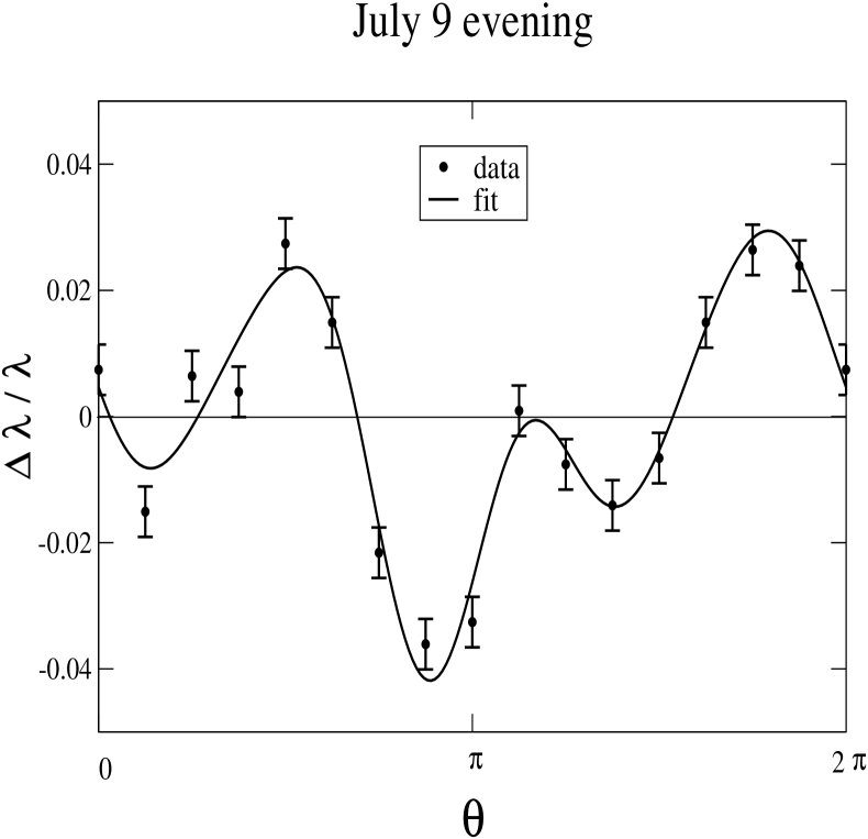
Figure 1: We show a typical fit eq.(4) to the Michelson-Morley data reported in Table 1.

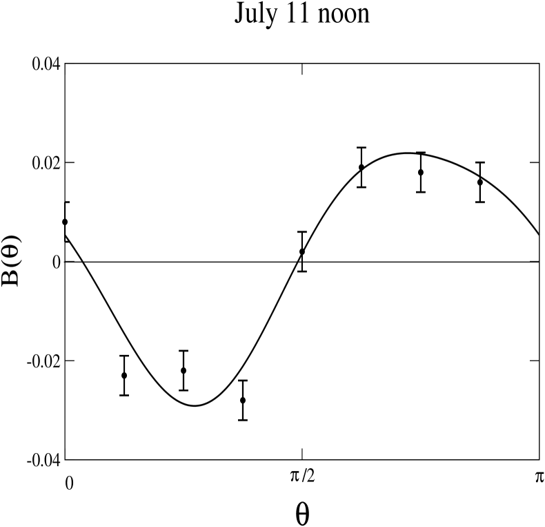
Figure 2: A typical fit eq.(4) to the even combination of fringe shifts $B(\theta)={{\Delta\lambda(\theta)+\Delta\lambda(\pi+\theta)}\over{2\lambda}}$ obtained from the data reported in Table 1. The fitted amplitudes are ${A}_{2}=0.025\pm 0.004$ and ${A}_{4}=0.004\pm 0.004$.

We have reported in table 2, our values of ${A}_{2}$ for each session. The individual determinations, that show good consistency, have been obtained from a 10-parameter fit to the various sets of 16 data (see fig.1) where, following Miller’s indications, the first five harmonics were included. To test the stability of these ${A}_{2}$ values, we have also fitted the even combination of fringe shifts ${{\Delta\lambda(\theta)+\Delta\lambda(\pi+\theta)}\over{2\lambda}}$. In this second type of fit, where only the even harmonics appear, the central values of ${A}_{2}$ come out exactly as in table 2 with slightly smaller errors ($\pm 0.004$ rather than $\pm 0.005$) and the fourth-harmonic component is consistent with the background (see fig.2).

While the individual values of $A_{2}$ show good consistency, there are large fluctuations in the values of $\phi_{2}$ for the various sessions. Their typical trend is in qualitative agreement with the values reported by Miller. For this comparison, see fig.22 of ref.[15], in particular the large scatter of the data taken around August 1st, as this represents the epoch of the year which is closest to the period of July when the Michelson-Morley observations were actually performed. Just this type of ‘erratic’ behaviour motivated Miller’s idea that a very large number of measurements, performed during the whole 24 hours of the day, was needed for a reliable determination of the azimuth of the ether-drift effect.

Concerning the extraction of the observable velocity, we note that for the Michelson-Morley apparatus where ${{D}\over{\lambda}}\sim 2\cdot 10^{7}$ [13], it becomes convenient to normalize the experimental values of ${A}_{2}$ to the classical prediction for an Earth’s velocity of 30 km/s

$${{D}\over{\lambda}}~{}{{(30{\rm km/s})^{2}}\over{c^{2}}}\sim 0.2$$ (6)

and we obtain

$$v_{\rm obs}\sim 30~{}\sqrt{{{A}_{2}}\over{0.2}}~{}~{}{\rm km/s}$$ (7)

Now, by inspection of table 2, we find that the average value of ${A}_{2}$ from the noon sessions, ${A}_{2}=0.017\pm 0.003$, indicates a velocity $v_{\rm obs}=8.7\pm 0.8$ km/s and the average value from the evening sessions, ${A}_{2}=0.014\pm 0.003$, indicates a velocity $v_{\rm obs}=8.0\pm 0.8$ km/s. Since the two determinations are well consistent with each other, we conclude that the Michelson-Morley experiment provides an average ${A}_{2}$ which is $\sim 1/13$ of the classical expectation and an average observable velocity $v_{\rm obs}\sim 8.4\pm 0.5~{}{\rm km/s}$ in excellent agreement with Miller’s analysis of the Michelson-Morley data.

On the other hand, the comparison with the interpretation that Michelson and Morley gave of their data is not so simple. First of all, they averaged the raw data from the various sessions so that the evidence for an ether-drift are unavoidably weaker. In addition, they do not quote any mean velocity but just start from the observation that “…the displacement to be expected was 0.4 fringe” while “…the actual displacement was certainly less than the twentieth part of this”. In this way, since the displacement is proportional to the square of the velocity, “…the relative velocity of the earth and the ether is… certainly less than one-fourth of the orbital earth’s velocity”.

The straightforward translation of this upper bound is $v_{\rm obs}<$ 7.5 km/s. However, even accepting their average of the raw data, their estimate is likely affected by a theoretical uncertainty. In fact, in their fig.6, Michelson and Morley reported their experimental fringe shifts together with the plot of a reference second-harmonic component. In doing so, they plotted a wave with amplitude $A_{2}=0.05$, that they interpret as one-eight of the theoretical displacement expected on the base of classical physics, thus implicitely assuming $A^{\rm class}_{2}$=0.4. As shown in eq.(6), the amplitude of the classically expected second-harmonic component is not 0.4 but is just one-half of that, i.e. 0.2. Therefore, their experimental upper bound $A^{\rm exp}_{2}<{{0.4}\over{20}}=$0.02, using our eq.(7), might also be interpreted as $v_{\rm obs}<$ 9.5 km/s, consistently with our estimate $v_{\rm obs}\sim 8.4\pm 0.5~{}{\rm km/s}$.

We conclude this section noticing that our Michelson-Morley value $v_{\rm obs}\sim 8.4\pm 0.5~{}{\rm km/s}$ is also in good agreement with the experimental results obtained by Miller himself at Mt. Wilson. As anticipated, differently from the original Michelson-Morley experiment, Miller’s data were taken over the entire day and in four epochs of the year. However, after the critical re-analysis of Shankland et al. [23], it turns out that the average daily determinations of ${A}_{2}$ for the four epochs were statistically consistent (see page 170 of ref.[23]). Therefore, one can average the four daily determinations, ${A}_{2}=0.044\pm 0.005$, and compare with the equivalent form of eq.(6) for the Miller’s interferometer ${{D}\over{\lambda}}~{}{{(30{\rm km/s})^{2}}\over{c^{2}}}\sim 0.56$. Again, the observed ${A}_{2}$ is $\sim 1/13$ of the classical expectation for an Earth’s velocity of 30 km/s and the effective $v_{\rm obs}$ is exactly the same as for the Michelson-Morley data.

This close agreement is also confirmed by another independent analysis. In fact, Múnera’s analysis [21] of the only Miller’s set of data explicitely reported in the literature yields the value $v_{\rm obs}=8.2\pm 1.4$ km/s (errors at the 95$\%$ C.L.), again in excellent agreement with our value for the Michelson-Morley experiment.

Therefore, by also taking into account the results obtained by Morley-Miller in the years 1902-1905, as shown in fig.4 of ref.[15], we conclude that the results of these three main classical ether-drift experiments can be summarized into the value

$$v_{\rm obs}\sim 8.5\pm 1.5~{}{\rm km/s}$$ (8)

3. The role of Lorentz transformations

Now, suppose we accept the value in eq.(8) to summarize the results of the Michelson-Morley, Morley-Miller and Miller experiments. As these were performed in air, it would mean that the measured two-way speed of light differs from an exactly isotropical value

$$u_{\rm air}={{c}\over{\cal{N}_{\rm air}}}$$ (9)

${\cal N}_{\rm air}$ denoting the refractive index of the air. Namely, for an observer placed on the Earth light is slightly anisotropical at a level ${\cal O}({{v^{2}_{\rm obs}}\over{c^{2}}})\sim 10^{-9}$ so that eq.(9) is only accurate at a lower level of accuracy, say $\sim 10^{-8}$.

On the other hand, for the Kennedy’s [24] experiment, where the whole optical system was inclosed in a sealed metal case containing helium at atmospheric pressure, the observed anisotropy was definitely smaller. In fact, the accuracy of the experiment, such to exclude fringe shifts as large as 1/4 of those expected on the base of eq.(8) (or 1/50 of that expected on the base of a velocity of 30 km/s) allows to place an upper bound $v_{\rm obs}<4$ km/s. This is confirmed by the re-analysis of the Illingworth’s experiment [25] performed by Múnera [21] who pointed out some incorrect assumptions in the original analysis of the data. From this re-analysis, the relevant observable velocity turns out to be $v_{\rm obs}=3.1\pm 1.0$ km/s (errors at the 95$\%$ C.L.) [21], with typical fringe shifts that were 1/100 of that expected for a velocity of 30 km/s. Again, this means that, for an apparatus filled with gaseous helium at atmospheric pressure, the measured two-way speed of light differs from the exactly isotropical value ${{c}\over{\cal{N}_{\rm helium}}}$ by terms ${\cal O}({{v^{2}_{\rm obs}}\over{c^{2}}})\sim 10^{-10}$.

Finally, for the Joos experiment [26], performed in an evacuated housing and where any ether-wind was found smaller than $1.5$ km/s, the typical value $v_{\rm obs}\sim 1$ km/s means that, in that particular type of vacuum, the fringe shifts were smaller than 1/400 of those expected for an Earth’s velocity of 30 km/s and the anisotropy of the two-way speed of light was at the level $\sim 10^{-11}$.

Tentatively, we shall try to summarize the above experimental results saying that when light propagates in a gaseous medium, the exactly isotropical value

$$u={{c}\over{\cal{N}_{\rm medium}}}$$ (10)

holds approximately for an observer placed on the Earth. Apparently, the observed trend is such that the anisotropy becomes smaller when the refractive index of the medium approaches unity. In fact $v_{\rm obs}$, and thus the anisotropy, is larger for those interferometers operating in air, where ${\cal N}_{\rm air}\sim 1.00029$, and becomes smaller in experiments performed in helium, where ${\cal N}_{\rm helium}\sim 1.000036$, or in an evacuated housing. This observation suggests to interpret the experiments adopting the point of view of ref.[7] that we shall briefly recapitulate in the following.

A small anisotropy of the two-way speed of light measured by an observer $S^{\prime}$ placed on the Earth, leads to consider, as in the pre-relativistic physics, the existence of a preferred reference frame $\Sigma$, where light propagates isotropically, and generate the anisotropy in $S^{\prime}$ as a consequence of the relative motion. This is similar to the conventional treatment of the Michelson-Morley experiment where one starts from the isotropical value $c$ in $\Sigma$ and uses Galileian relativity (for which the speed of light becomes $c\pm v$) to transform to the observer $S^{\prime}$ placed in the Earth’s frame.

In doing so, however, one neglects i) that light may propagate in a dielectric medium and ii) that Galilei’s trasformations have to be replaced by Lorentz transformations. These preserve the value of the speed of light in the vacuum $c=2.9979...\cdot 10^{10}$ cm/s but do not preserve its isotropical value in a medium. In this case, one has to account for a non-vanishing Fresnel’s drag coefficient

$$k_{\rm medium}=1-{{1}\over{{\cal N}^{2}_{\rm medium}}}\ll 1$$ (11)

Therefore, to generate an anisotropy in $S^{\prime}$ one can start from eq.(10), assumed to be valid in $\Sigma$, and apply a Lorentz transformation. By denoting ${\bf{v}}$ the velocity of $S^{\prime}$ with respect to $\Sigma$, the general Lorentz transformation that gives the one-way speed of light in $S^{\prime}$ is ($\gamma=1/\sqrt{1-{{{\bf{v}}^{2}}\over{c^{2}}}}$)

$${\bf{u}}^{\prime}={{{\bf{u}}-\gamma{\bf{v}}+{\bf{v}}(\gamma-1){{{\bf{v}}\cdot{\bf{u}}}\over{v^{2}}}}\over{\gamma(1-{{{\bf{v}}\cdot{\bf{u}}}\over{c^{2}}})}}$$ (12)

where $v=|{\bf{v}}|$. By keeping terms up to second order in $v/u$, denoting by $\theta$ the angle between ${\bf{v}}$ and ${\bf{u}}$ and defining $u^{\prime}(\theta)=|{\bf{u^{\prime}}}|$, we obtain

$${{u^{\prime}(\theta)}\over{u}}=1-\alpha{{v}\over{u}}-\beta{{v^{2}}\over{u^{2}}}$$ (13)

where

$$\alpha=k_{\rm medium}\cos\theta+{\cal O}(k^{2}_{\rm medium})$$ (14)

$$\beta=k_{\rm medium}P_{2}(\cos\theta)+{\cal O}(k^{2}_{\rm medium})$$ (15)

with $P_{2}(\cos\theta)={{1}\over{2}}(3\cos^{2}\theta-1)$.

Finally, the two-way speed of light is

$${{\bar{u}^{\prime}(\theta)}\over{u}}={{1}\over{u}}~{}{{2u^{\prime}(\theta)u^{\prime}(\pi+\theta)}\over{u^{\prime}(\theta)+u^{\prime}(\pi+\theta)}}=1-{{v^{2}}\over{c^{2}}}(A+B\sin^{2}\theta)$$ (16)

where

$$A=k_{\rm medium}+{\cal O}(k^{2}_{\rm medium})$$ (17)

and

$$B=-{{3}\over{2}}k_{\rm medium}+{\cal O}(k^{2}_{\rm medium})$$ (18)

In this way, as shown in ref.[7], one obtains formally the same pre-relativistic expressions where the kinematical velocity $v$ is replaced by an effective observable velocity

$$v_{\rm obs}=v\sqrt{k_{\rm medium}}\sqrt{3}\sim v\sqrt{-2B}$$ (19)

For instance, for the Michelson-Morley experiment, and for an ether wind along the $x$ axis, the $S^{\prime}$-prediction for the fringe shifts at a given angle $\theta$ with the $x$ axis has the particularly simple form ($D$ being the length for $S^{\prime}$ of each arm of the interferometer)

$${{\Delta\lambda(\theta)}\over{\lambda}}={{u}\over{\lambda}}({{2D}\over{\bar{u^{\prime}}(\theta)}}-{{2D}\over{\bar{u^{\prime}}(\pi/2+\theta)}})\sim{{D}\over{\lambda}}{{v^{2}}\over{c^{2}}}(-2B)\cos(2\theta)={{D}\over{\lambda}}{{v^{2}_{\rm obs}}\over{c^{2}}}\cos(2\theta)$$ (20)

that corresponds to a pure second-harmonic effect as in eq.(5) where $v^{2}$ is replaced by $v^{2}_{\rm obs}$. Notice that, as discussed in the Introduction, in agreement with the basic isotropy of space, the measured length of an interferometer at rest in $S^{\prime}$ is $D$ regardless of the angle $\theta$ of its orientation.

We observe that eqs.(19) and (20) provide a clear-cut argument to understand why the fringe shifts were coming out much smaller than classically expected: they are proportional to the squared Earth’s velocity through the Fresnel’s drag coefficient of the dielectric medium used in the interferometer. Thus, there should be no surprise that the ‘observable’ velocity is much smaller than the ‘kinematical’ velocity.

Also, the trend predicted by eqs.(19) and (20) is such to reproduce correctly the experimental results. In fact, the observable velocity, and thus the anisotropy, becomes smaller and smaller when ${\cal N}_{\rm medium}$ approaches unity and vanishes identically in the limit ${\cal N}_{\rm medium}\to 1$. This is consistent with the analysis of the experiments performed by Kennedy, Illingworth and Joos vs. those of Michelson-Morley, Morley-Miller and Miller. We note that a qualitatively similar suppression effect had already been discovered by Cahill and Kitto [27] by following a different approach.

4. Interpretation of the classical ether-drift experiments

Now, if upon operation of the interferometer there are fringe shifts and if their magnitude, observed with different dielectric media and within the experimental errors, points consistently to a unique value of the kinematical Earth’s velocity, there is experimental evidence for the existence of a preferred frame $\Sigma\neq S^{\prime}$. In practice, to ${\cal O}({{v^{2}_{\rm earth}}\over{c^{2}}})$, this can be decided by re-analyzing the experiments in terms of the effective parameter $\epsilon={{v^{2}_{\rm earth}}\over{u^{2}}}k_{\rm medium}$. The conclusion of Cahill and Kitto [27] is that the classical experiments are consistent with the value $v_{\rm earth}\sim 365$ km/s obtained from the dipole fit to the COBE data [28] for the anisotropy of the cosmic background radiation.

However, in our expression eq.(19) determining the fringe shifts there is a difference of a factor $\sqrt{3}$ with respect to their result $v_{\rm obs}=v\sqrt{k_{\rm medium}}$. Therefore, using eqs.(19) and (8), for ${\cal N}_{\rm air}\sim 1.00029$, the relevant Earth’s velocity (in the plane of the interferometer) is not $v_{\rm earth}\sim 365$ km/s but rather

$$v_{\rm earth}\sim 204\pm 36~{}{\rm km/s}$$ (21)

This value provides a definite range of velocities that can be used in the analysis of the other experiments.

To this end, let us compare with the experiment performed by Michelson, Pease and Pearson [29]. These other authors in 1929, using their own interferometer, again at Mt. Wilson, declared that their “precautions taken to eliminate effects of temperature and flexure disturbances were effective”. Therefore, their statement that the fringe shift, as derived from “…the displacements observed at maximum and minimum at sidereal times…”, was definitely smaller than “…one-fifteenth of that expected on the supposition of an effect due to a motion of the Solar System of three hundred kilometres per second”, can be taken as an indirect confirmation of our eq.(21). Indeed, although the “one-fifteenth” was actually a “one-fiftieth” (see page 240 of ref.[15]), their fringe shifts were certainly non negligible. This is easily understood since, for an in-air-operating interferometer, the fringe shift $(\Delta\lambda)_{\rm class}(300)$, expected on the base of classical physics for an Earth’s velocity of 300 km/s, is about 500 times bigger than the corresponding relativistic one

$$(\Delta\lambda)_{\rm rel}(300)\equiv 3k_{\rm air}~{}(\Delta\lambda)_{\rm class}(300)$$ (22)

computed using Lorentz transformations (compare with eq.(20) for $k_{\rm air}\sim{\cal N}^{2}_{\rm air}-1\sim 0.00058$). Therefore, the Michelson-Pease-Pearson upper bound

$$(\Delta\lambda)_{\rm obs}<0.02~{}(\Delta\lambda)_{\rm class}(300)$$ (23)

is actually equivalent to

$$(\Delta\lambda)_{\rm obs}<24~{}(\Delta\lambda)_{\rm rel}(204)$$ (24)

As such, it poses no strong restrictions and is entirely consistent with those typical low observable velocities reported in eq.(8).

A similar agreement is obtained when comparing with the Illingworth’s data [25] as recently re-analyzed by Múnera [21]. In this case, using eq.(19), the observable velocity $v_{\rm obs}=3.1\pm 1.0$ km/s [21] (errors at the 95$\%$ C.L.) and the value ${\cal N}_{\rm helium}-1\sim 3.6\cdot 10^{-5}$, one deduces $v_{\rm earth}=213\pm 36$ km/s (errors at the 68$\%$ C.L.) in very good agreement with our eq.(21).

The same conclusion applies to the Joos experiment [26]. Although we don’t know the exact value of ${\cal N}_{\rm vacuum}$ for the Joos experiment, it is clear that his result, $v_{\rm obs}<$ 1.5 km/s, represents the natural type of upper bound in this case. As an example, for $v_{\rm earth}\sim 204$ km/s, one obtains $v_{\rm obs}\sim 1.5$ km/s for ${\cal N}_{\rm vacuum}-1=9\cdot 10^{-6}$ and $v_{\rm obs}\sim 0.5$ km/s for ${\cal N}_{\rm vacuum}-1=1\cdot 10^{-6}$. In this sense, the effect of using Lorentz transformations is most dramatic for the Joos experiment when comparing with the classical expectation for an Earth’s velocity of 30 km/s. Although the relevant Earth’s velocity can be as large as $204$ km/s, the fringe shifts, rather than being $(204/30)^{2}\sim 50$ times bigger than the classical prediction, are $\sim(30/1.5)^{2}=400$ times smaller.

Notice that, using our eq.(19), the kinematical Earth’s velocity obtained from the absolute magnitude of the fringe shifts becomes consistent with that needed by Miller to understand the variations of the ether-drift effect in different epochs of the year [15]. In fact, the typical daily values, in the plane of the interferometer, had to lie in the range 195 km/s$\leq v_{\rm earth}\leq 211$ km/s (see table V of ref.[15]). Such a consistency, on one hand, increases the body of experimental evidence for a preferred frame, and on the other hand, signals the internal consistency of Miller’s analysis.

We are aware that our conclusion goes against the widely spread belief, originating from the paper of Shankland et al. ref.[23], that Miller’s results were actually due to statistical fluctuation and/or local temperature conditions. To a closer look, however, the argument of Shankland et al. is not so solid as it appears by reading the Abstract of their paper. In fact, within the paper these authors say that “…there can be little doubt that statistical fluctuations alone cannot account for the periodic fringe shifts observed by Miller” (see page 171 of ref.[23]). In fact, although “…there is obviously considerable scatter in the data at each azimuth position,…the average values…show a marked second harmonic effect” (see page 171 of ref.[23]). In any case, interpreting the observed effects on the base of the local temperature conditions is certainly not the only explanation since “…we must admit that a direct and general quantitative correlation between amplitude and phase of the observed second harmonic on the one hand and the thermal conditions in the observation hut on the other hand could not be established” (see page 175 of ref.[23]). This rather unsatisfactory explanation of the observed effects should be compared with the previously mentioned excellent agreement that was instead obtained by Miller once the final parameters for the Earth’s velocity were plugged in the theoretical predictions (see figs.26 and 27 of ref.[15]).

The most surprising thing, however, is that Shankland et al. did not realize that Miller’s average value ${A}_{2}=0.044\pm 0.005$, obtained after their own critical re-analysis of his observations at Mt.Wilson, when compared to the expected classical value $A_{2}=0.56$ for his interferometer, was giving precisely the same $v_{\rm obs}\sim 8.4\pm 0.5$ km/s obtained from the Miller’s re-analysis of the Michelson-Morley experiment in Cleveland. Conceivably, their emphasis on the role of the temperature effects in the Miller’s data would have been re-considered whenever they had realized the perfect identity of two determinations obtained in completely different experimental conditions.

5. Comparison with present-day experiments

Let us finally consider those present-day, ‘high vacuum’ Michelson-Morley experiments of the type first performed by Brillet and Hall [17] and more recently by Müller et al. [18]. In these experiments, the test of the isotropy of the speed of light does not consist in the observation of the interference fringes as in the classical experiments. Rather, one looks for the difference $\Delta\nu$ in the relative frequencies of two cavity-stabilized lasers upon local rotations of the apparatus [17] or under the Earth’s rotation [18] on the base of the relation

$$\nu(\theta)={{\bar{u}^{\prime}(\theta)n}\over{2L}}$$ (25)

Here $\bar{u}^{\prime}(\theta)$ is the two-way speed of light within the cavity, $n$ is the integer number fixing the cavity mode and $L$ the length of the cavity as measured in $S^{\prime}$. Again, as stressed in connection with eq.(20), due to the isotropy of space the cavity length is taken to be independent of the cavity orientation.

The present experimental value for the anisotropy of the two-way speed of light in the vacuum, as determined by Müller et al.[18],

$${{\Delta\nu_{\theta}}\over{\nu}}=({{\Delta\bar{c}_{\theta}}\over{c}})_{\rm exp}=(2.6\pm 1.7)\cdot 10^{-15}$$ (26)

can be interpreted within the framework of our eq.(16) where

$$({{\Delta\bar{c}_{\theta}}\over{c}})_{\rm theor}\sim|B_{\rm vacuum}|{{v^{2}_{\rm earth}}\over{c^{2}}}$$ (27)

Now, in a perfect vacuum by definition ${\cal N}_{\rm vacuum}=1$ so that $B_{\rm vacuum}$ and $v_{\rm obs}$ vanish. However, one can explore [7] the possibility that, even in this case, a very small anisotropy might be due to a refractive index ${\cal N}_{\rm vacuum}$ that differs from unity by an infinitesimal amount. In this case, the natural candidate to explain a value ${\cal N}_{\rm vacuum}\neq 1$ is gravity. In fact, by using the Equivalence Principle, a freely falling frame $S^{\prime}$ will locally measure the same speed of light as in an inertial frame in the absence of any gravitational effect. However, if $S^{\prime}$ carries on board an heavy object this is no longer true. For an observer placed on the Earth, this amounts to insert the Earth’s gravitational potential in the weak-field isotropic approximation to the line element of General Relativity [30]

$$ds^{2}=(1+2\varphi)dt^{2}-(1-2\varphi)(dx^{2}+dy^{2}+dz^{2})$$ (28)

so that one obtains a refractive index for light propagation

$${\cal N}_{\rm vacuum}\sim 1-2\varphi$$ (29)

This represents the ‘vacuum analogue’ of ${\cal N}_{\rm air}$, ${\cal N}_{\rm helium}$,…so that from

$$\varphi=-{{G_{N}M_{\rm earth}}\over{c^{2}R_{\rm earth}}}\sim-0.7\cdot 10^{-9}$$ (30)

and using eq.(18) one predicts

$$B_{\rm vacuum}\sim-4.2\cdot 10^{-9}$$ (31)

Adopting the range of Earth’s velocity (in the plane of the interferometer) given in eq.(21) this leads to predict an observable anisotropy of the two-way speed of light in the vacuum eq.(16)

$$({{\Delta\bar{c}_{\theta}}\over{c}})_{\rm theor}\sim|B_{\rm vacuum}|{{v^{2}_{\rm earth}}\over{c^{2}}}\sim(1.9\pm 0.7)\cdot 10^{-15}$$ (32)

consistently with the experimental value in eq.(26).

Clearly, in this framework, trying to rule out the existence of a preferred frame through the experimental determination of ${{\Delta\bar{c}_{\theta}}\over{c}}$ in a high vacuum is not the most convenient strategy due to the vanishingly small value of $B_{\rm vacuum}$. In other words, even with years of data taking [18], it is not easy to rule out the theoretical prediction in eq.(32) starting from the present experimental value eq.(26).

For this reason, a more efficient search might be performed in dielectric gaseous media where, if there is a preferred frame, the frequency of the signal should be much larger. As a check, we have compared with the only available results obtained by Jaseja et. al [19] in 1963 when looking at the relative frequency shifts of two orthogonal He-Ne masers placed on a rotating platform. As we shall show in the following, their data are consistent with the same type of conclusion obtained from the classical experiments: an ether-drift effect determined by an Earth’s velocity as in eq.(21).

To use the experimental results reported by Jaseja et al.[19] one has to subtract preliminarly a large overall systematic effect that was present in their data and interpreted by the authors as probably due to magnetostriction in the Invar spacers induced by the Earth’s magnetic field. As suggested by the same authors, this spurious effect, that was only affecting the normalization of the experimental $\Delta\nu$, can be subtracted looking at the variations of the data at different hours of the day. The data for $\Delta\nu$, in fact, in spite of their rather large errors, exhibit a characteristic modulation (see fig.3 of ref.[19]) with a maximum at about 7:30 a.m. and a minimum at about 9:00 a.m.. To estimate the size of the time modulation, one can follow two different strategies: a) just consider the two data corresponding to the maximal and minimal values $\Delta\nu_{\rm exp}(7:30~{}{\rm a.m.})\sim 276\pm 5$ kHz, $\Delta\nu_{\rm exp}(9:00~{}{\rm a.m.})\sim 267\pm 4$ kHz and the difference

$$\delta_{a}(\Delta\nu)\equiv\Delta\nu_{\rm exp}(7:30~{}{\rm a.m.})-\Delta\nu_{\rm exp}(9:00~{}{\rm a.m.})\sim(9\pm 6)~{}{\rm kHz}$$ (33)

or b), following Jaseja et al., group the data in two bins of six by defining average values, say $\langle\Delta\nu\rangle_{\rm exp}(7:30~{}{\rm a.m.})$ and $\langle\Delta\nu\rangle_{\rm exp}(9:00~{}{\rm a.m.})$, thus obtaining

$$\delta_{b}(\Delta\nu)\equiv\langle\Delta\nu\rangle_{\rm exp}(7:30~{}{\rm a.m.})-\langle\Delta\nu\rangle_{\rm exp}(9:00~{}{\rm a.m.})\sim(1.6\pm 1.2)~{}{\rm kHz}$$ (34)

Our theoretical starting point to understand the above (rather loose) determinations is the formula for the frequency shift of the two masers at an angle $\theta$ with the direction of the ether-drift

$${{\Delta\nu(\theta)}\over{\nu}}={{\bar{u}^{\prime}(\pi/2+\theta)-\bar{u}^{\prime}(\theta)}\over{u}}=|B_{\rm He-Ne}|{{v^{2}_{\rm earth}}\over{c^{2}}}\cos(2\theta)$$ (35)

where, taking into account the values ${\cal N}_{\rm helium}\sim 1.000036$, ${\cal N}_{\rm neon}\sim 1.000067$, ${\cal N}_{\rm He-Ne}\sim 1.00004$ and eq.(18) we shall use $|B_{\rm He-Ne}|\sim 1.2\cdot 10^{-4}$.

Further, using the value of the frequency of ref.[19] $\nu\sim 3\cdot 10^{14}$ Hz and our standard value eq.(21) for the Earth’s velocity in the plane of the interferometer $v_{\rm earth}\sim 200$ km/s, eq.(35) leads to the reference value for the amplitude of the signal

$$(\Delta\nu)_{\rm ref}=\nu|B_{\rm He-Ne}|{{(200~{}{\rm km/s})^{2}}\over{c^{2}}}\sim 16~{}{\rm kHz}$$ (36)

and to its time modulation

$$\delta(\Delta\nu)_{\rm theor}\sim 16~{}{\rm kHz}~{}{{\delta v^{2}}\over{v^{2}}}$$ (37)

where

$${{\delta v^{2}}\over{v^{2}}}\equiv{{v^{2}_{\rm earth}(7:30~{}{\rm a.m.})-v^{2}_{\rm earth}(9:00~{}{\rm a.m.})}\over{(200~{}{\rm km/s})^{2}}}$$ (38)

To evaluate the above ratio of velocities, let us first compare the modulation of $\Delta\nu$ seen in fig.3 of ref.[19] with that of $v_{\rm obs}$ in fig.27 of ref.[15] (data plotted as a function of civil time as in ref.[19]) restricting to the Miller’s data of February, the period of the year that is closer to the date of January 20th when Jaseja et al. performed their experiment. Further, the different location of the two laboratories (Mt.Wilson and Boston) can be taken into account with a shift of about three hours so that Miller’s interval 3:00 a.m.$-$9:00 a.m. is made to correspond to the range 6:00 a.m.$-$12:00 a.m. of Jaseja et al.. If this is done, although one does not expect an exact correspondence due to the difference between the two epochs of the year, the two characteristic trends are surprisingly close.

Thus we shall try to use the Miller’s data for a rough evaluation of the ratio reported in eq.(38) after rescaling from $v_{\rm obs}$ to $v_{\rm earth}$ through eq.(19) (for the Miller’s interferometer that was operating in air). Following for the Miller’s data the same procedure used to obtain eq.(33) (i.e. just restricting to the difference between maximal and minimal values) we obtain a maximal observable velocity $(v_{\rm obs})^{\rm max}\sim 9.4$ km/s, that corresponds to a value $(v_{\rm earth})^{\rm max}\sim 225$ km/s, and a minimal observable velocity $(v_{\rm obs})^{\rm min}\sim 7.5$ km/s, that corresponds to a value $(v_{\rm earth})^{\rm min}\sim 180$ km/s. These velocities, when replaced in eq.(38), produce a value ${{(\delta v^{2})_{a}}\over{v^{2}}}\sim 0.46$ that, when used in eq.(37), leads to a theoretical prediction $\delta(\Delta\nu)_{\rm theor}\sim 7.3$ kHz, well consistent with the experimental result in eq.(33). On the other hand, averaging the Miller’s data slightly to the left and to the right of the minimum, we get the smaller value ${{(\delta v^{2})_{b}}\over{v^{2}}}\sim 0.12$ that, when replaced in eq.(37), leads to $\delta(\Delta\nu)_{\rm theor}\sim 1.8$ kHz consistently with eq.(34). Of course, for a really significative test, one needs more precise data. However, with the present data eqs.(33) and (34), and in spite of our crude approximations, the order of magnitude of the effect is correctly reproduced.

This suggests, once more [7], to perform a new class of ether-drift experiments in dielectric gaseous media. For instance, using stabilizing cavities as in Refs.[17, 18], one could replace the high vacuum in the Fabry-Perot with air. In this case, where $|B_{\rm vacuum}|\sim 4\cdot 10^{-9}$ would be replaced by $|B_{\rm air}|\sim 9\cdot 10^{-4}$, there should be an increase by five orders of magnitude in the typical value of $\Delta\nu$ with respect to refs.[17, 18].

6. Summary and outlook

In this paper we have re-considered the possible existence of a preferred reference frame through an analysis of the classical and modern ether-drift experiments. Our re-analysis started with the original data obtained by Michelson and Morley [13] in each session of their experiment. Contrary to the generally accepted ideas, but in agreement with the point of view expressed by Hicks in 1902 [14], Miller in 1933 [15] and Múnera in 1998 [21], the results of that experiment should not be considered null. The even combinations of fringe shifts ${{\Delta\lambda(\theta)+\Delta\lambda(\pi+\theta)}\over{2\lambda}}$, although smaller than the classical prediction corresponding to the orbital motion of the Earth, exhibit the characteristic second-harmonic behaviour (see fig.2) expected for an ether-drift effect. The average amplitude of the second-harmonic component ${A}_{2}\sim 0.016\pm 0.002$ (see table 2), when normalized to the expected classical value ${{D}\over{\lambda}}~{}{{(30{\rm km/s})^{2}}\over{c^{2}}}\sim 0.2$ for the Michelson-Morley interferometer, corresponds to an average observed velocity $v_{\rm obs}\sim 8.4\pm 0.5$ km/s.

As emphasized at the end of Sect.2 and at the end of Sect.4, this average value of $v_{\rm obs}$ for the Michelson-Morley experiment is exactly the same average daily value that was obtained by Miller in his 1925-1926 observations at Mt.Wilson. This can easily be checked, after the critical re-analysis of Shankland et al., by comparing Miller’s average daily value ${A}_{2}\sim 0.044\pm 0.005$ (see page 170 of ref.[23]) with the expected classical value ${{D}\over{\lambda}}~{}{{(30{\rm km/s})^{2}}\over{c^{2}}}\sim 0.56$ for the Miller’s interferometer.

Our conclusion is further confirmed by the independent analysis of the available Miller’s data performed by Múnera [21] which provides the value $v_{\rm obs}\sim 8.2\pm 1.4$ km/s. By including the other determinations obtained by Morley and Miller in the period 1902-1905 (see fig.4 of ref.[15]), the results of these three main classical ether-drift experiments can be summarized in the value $v_{\rm obs}\sim 8.5\pm 1.5$ km/s.

Therefore, once different ether-drift experiments give consistent values of the Earth’s observable velocity, it becomes natural to explore the existence of a preferred frame, within the context of Lorentzian Relativity, and use Lorentz transformations to extract the real kinematical velocity corresponding to this $v_{\rm obs}$. In this case, using eq.(19), we find a value (in the plane of the interferometer) $v_{\rm earth}\sim 204\pm 36$ km/s in agreement with the range 195 km/s $\leq v_{\rm obs}\leq$ 211 km/s needed by Miller to describe the variations of the ether-drift effect in different epochs of the year (see table V of ref.[15]).

At the same time, using Lorentz transformations, the same range of $v_{\rm earth}$ corresponds to an effective $v_{\rm obs}\sim 3$ km/s for the Kennedy’s [24] and Illingworth [25] experiments (performed in helium) or $\sim 1$ km/s for the Joos experiment [26] (performed in an evacuated housing) consistently with the experimental results.

Additional checks of this theoretical framework are obtained by comparing with the experimental data for the relative frequency shift $\Delta\nu$ which is measured in the present-day experiments with cavity-stabilized lasers, upon local rotation of the apparatus or under the Earth’s rotation. In this case, our basic relation is

$${{\Delta\nu}\over{\nu}}\sim|B_{\rm medium}|{{v^{2}_{\rm earth}}\over{c^{2}}}$$ (39)

where $B_{\rm medium}\sim-3({\cal N}_{\rm medium}-1)$, ${\cal N}_{\rm medium}$ being the refractive index of the gaseous dielectric medium that fills the cavities. For a very high vacuum, using the prediction of General Relativity for an apparatus placed on the Earth’s surface, $|B_{\rm vacuum}|\sim 4\cdot 10^{-9}$, and the range of kinematical Earth’s velocity $v_{\rm earth}\sim 204\pm 36$ km/s suggested by the classical ether-drift experiments, we predict $({{\Delta\nu}\over{\nu}})_{\rm theor}\sim(1.9\pm 0.7)\cdot 10^{-15}$, consistently with the experimental result $({{\Delta\nu}\over{\nu}})_{\rm exp}=(2.6\pm 1.7)\cdot 10^{-15}$ obtained in ref.[18].

For He-Ne masers, the same range of Earth’s velocities leads to predict a typical value $\Delta\nu\sim 16$ kHz, for which ${{\Delta\nu}\over{\nu}}\sim 5\cdot 10^{-11}$, with a characteristic modulation of a few kHz in the period of the year and for the hours of the day when Jaseja et al.[19] performed their experiment. This prediction is consistent with their data, although the rather large experimental errors require further experimental checks. To this end, an efficient search for a preferred frame requires a modified experimental set-up where the high vacuum adopted in the resonating cavities is replaced by air. In this case, where the anisotropy parameter $|B_{\rm vacuum}|\sim 4\cdot 10^{-9}$ would be replaced by $|B_{\rm air}|\sim 9\cdot 10^{-4}$, there should be an increase of five orders of magnitude in the typical value of $\Delta\nu$ with respect to Refs.[17, 18]. If such enhancement is not observed, rather than waiting for years, the existence of a preferred frame will be definitely ruled out in a few days of data taking.

i	July 8 (n.)	July 9 (n.)	July 11 (n.)	July 8 (e.)	July 9 (e.)	July 12 (e.)
1	-0.001	+0.018	+0.015	-0.016	+0.007	+0.034
2	+0.024	-0.004	-0.035	+0.008	-0.015	+0.042
3	+0.053	-0.004	-0.039	-0.010	+0.006	+0.045
4	+0.015	-0.003	-0.067	+0.070	+0.004	+0.025
5	-0.036	-0.031	-0.043	+0.041	+0.027	-0.004
6	-0.007	-0.020	-0.015	+0.055	+0.015	-0.014
7	+0.024	-0.025	-0.001	+0.057	-0.022	+0.005
8	+0.026	-0.021	+0.027	+0.029	-0.036	-0.013
9	-0.021	-0.049	+0.001	-0.005	-0.033	-0.030
10	-0.022	-0.032	-0.011	+0.023	+0.001	-0.066
11	-0.031	+0.001	-0.005	+0.005	-0.008	-0.093
12	-0.005	+0.012	+0.011	-0.030	-0.014	-0.059
13	-0.024	+0.041	+0.047	-0.034	-0.007	-0.040
14	-0.017	+0.042	+0.053	-0.052	+0.015	+0.038
15	-0.002	+0.070	+0.037	-0.084	+0.026	+0.057
16	+0.022	-0.005	+0.005	-0.062	+0.024	+0.041
17	-0.001	+0.018	+0.015	-0.016	+0.007	+0.034

Table 1: We report the fringe shifts ${{\Delta\lambda(i)}\over{\lambda}}$ for all noon (n.) and evening (e.) sessions of the Michelson-Morley experiment.

.

SESSION	${A}_{2}$
July 8 (noon)	$0.010\pm 0.005$
July 9 (noon)	$0.015\pm 0.005$
July 11 (noon)	$0.025\pm 0.005$
July 8 (evening)	$0.014\pm 0.005$
July 9 (evening)	$0.011\pm 0.005$
July 12 (evening)	$0.018\pm 0.005$

Table 2: We report the amplitude of the second-harmonic component ${A}_{2}$ obtained from the fit eq.(4) to the various samples of data.

References

- [1] EINSTEIN A.: Ann. der Physik, 17, (1905) 891. English Translation in The Principle Of Relativity, (Dover Publications Inc.) 1952, p. 37.
- [2] LORENTZ H. A.: Electromagnetic phenomena in a system moving with any velocity less than that of light, Proceedings of the Academy of Sciences of Amsterdam, 6, 1904; in The Theory of Electrons, B. G. Teubner, Ed. Leipzig, 1909.
- [3] POINCARÉ H.: in La Science et l’Hypothese, Flammarion, Paris 1902; Comptes Rendue, 140, (1905) 1504.
- [4] MARTIN T.: gr-qc/0006029 Preprint 2000.
- [5] HARDY L.: Phys. Rev. Lett., 68, (1992) 2981.
- [6] SCARANI V. et al.: Phys. Lett., A 276, (2000) 1.
- [7] CONSOLI M., PAGANO A. AND PAPPALARDO L.: Phys. Lett., A318, (2003) 292.
- [8] VOLOVIK G. E.: JETP Lett., 73,(2001) 162.
- [9] STEVENSON P. M.: Are there pressure waves in the vacuum ?, in Conference on Violations of CPT and Lorentz Invariance, University of Indiana, August 2001, World Scientific, Singapore, hep-ph/0109204.
- [10] CONSOLI M.: Phys. Rev., D 65, (2002) 105017; Phys. Lett., B 541, (2002) 307.
- [11] BELL J. S.: How to teach special relativity in Speakable and unspeakable in quantum mechanics, Cambridge University Press 1987, pp. 67-80.
- [12] BROWN H. R. AND POOLEY O.: The origin of the space-time metric: Bell’s Lorentzian pedagogy and its significance in general relativity, in Physics meets Philosophy at the Planck Scale, edited by C. CALLENDER and N. HUGGET (Cambridge University Press) 2000 (gr-qc/9908048).
- [13] MICHELSON A.A. AND MORLEY E.W.: Am. J. Sci., 34, (1887) 333.
- [14] HICKS W. M.: Phil. Mag., 3, (1902) 9.
- [15] MILLER D.C.: Rev. Mod. Phys., 5, (1933) 203.
- [16] MORLEY E.W. AND MILLER D.C.: Phil. Mag., 9, (1905) 669.
- [17] BRILLET A. AND HALL J.L.: Phys. Rev. Lett., 42, (1979) 549.
- [18] MÜLLER H. et al.: Phys. Rev. Lett., 91, (2003) 020401.
- [19] JASEJA T.S. et al.: Phys. Rev., 133, (1964) A1221 .
- [20] HANDSCHY M.: Am. J. Phys., 50, (1982) 987.
- [21] MÚNERA H.A.: APEIRON, 5, (1998) 37.
- [22] KENNEDY R.J.: Phys. Rev., 47, (1935) 965.
- [23] SHANKLAND R.S. et al.: Rev. Mod. Phys., 27, (1955) 167.
- [24] KENNEDY R.J.: in Conference on The Michelson-Morley Experiment, Astrophys. Journ., 68, (1928) 341.
- [25] ILLINGWORTH K.K.: Phys. Rev., 30, (1927) 692.
- [26] JOOS G.: Ann. d. Physik, 7, (1930) 385.
- [27] CAHILL R.T. AND KITTO K.: physics/0205070 Preprint 2002.
- [28] SMOOT G.F. et al.: Astrophys.Journ., 371, (1991) L1.
- [29] MICHELSON A.A., PEASE F.G. AND PEARSON F.: Nature, 123, (1929) 88.
- [30] WEINBERG S.: in Gravitation and Cosmology, (John Wiley and Sons Inc.) 1972, p. 181.