Inhomogeneous Gravity

Abstract

We study the inhomogeneous cosmological evolution of the Newtonian gravitational ’constant’ $G$ in the framework of scalar-tensor theories. We investigate the differences that arise between the evolution of $G$ in the background universes and in local inhomogeneities that have separated out from the global expansion. Exact inhomogeneous solutions are found which describe the effects of masses embedded in an expanding FRW Brans-Dicke universe. These are used to discuss possible spatial variations of $G$ in different regions. We develop the technique of matching different scalar-tensor cosmologies of different spatial curvature at a boundary. This provides a model for the linear and non-linear evolution of spherical overdensities and inhomogeneities in $G.$ This allows us to compare the evolution of $G$ and $\dot{G}$ that occurs inside a collapsing overdense cluster with that in the background universe. We develop a simple virialisation criterion and apply the method to a realistic lambda-CDM cosmology containing spherical overdensities. Typically, far slower evolution of $\dot{G}$ will be found in the bound virialised cluster than in the cosmological background. We consider the behaviour that occurs in Brans-Dicke theory and in some other representative scalar-tensor theories.

1 Introduction

Many of the most interesting extensions of the general theory of relativity are scalar-tensor theories of gravity. They incorporate scalar fields which can carry space-time variations in scalar quantities that are traditionally assumed to be constant in general relativity. In this respect they provide natural arenas in which to explore the consequences of varying ’constants’ of Nature, like Newton’s ’constant’ $G$, or Sommerfeld’s fine structure ’constant’, $\alpha.$ In this paper we shall focus upon the first of these applications, pioneered by Jordan (Jordan, 1949, 1955, 1959) and then refined into the most familiar generalisation of Einstein’s theory of gravitation by Brans and Dicke in 1961, (Brans & Dicke, 1961). This theory features both in direct explorations of the possible variation of $G$, in dimensional reduction of higher-dimensional theories, and in string theories (Green, Schwartz & Witten, 1987), where is appears containing a dilaton with non-minimal coupling. The original theory of Brans-Dicke is recognised as the simplest case of a family of scalar-tensor gravity theories in which the original Brans-Dicke coupling parameter, $\omega$, becomes a function of the scalar field that carries variations in $G$, (Bergmann, 1968),(Wagoner, 1970; Nordtvedt, 1970).

Extensive studies have been made of cosmological solutions of scalar-tensor gravity theories (Fuji & Maeda, 2003), although they are limited in two respects. First, they focus on the simplest case of isotropic expansion with zero spatial curvature, where simple exact solutions exist. Second, they are exclusively concerned with spatially homogeneous cosmologies. The latter restriction means that the value of $G$ and its rate of change in time, $\dot{G},$ are required to be the same everywhere in the universe. This assumption has run through the entire literature on varying $G$ and so it is generally assumed, for example, that local observational bounds on varying $G$ derived from geophysics, solar system dynamics, stellar evolution, or white dwarf cooling can be applied directly to constrain cosmological variations in $G$ on extragalactic scales or in the very early universe. There is no justification for this simplifying assumption, as pointed out by Barrow and O’Toole (Barrow & O’Toole, 2001). The local bounds on varying $G$ are all derived from observations of gravitationally bound ’lumps’ which are in gravitational equilibrium and do not take part in the expansion of the universe. Before they can be extrapolated to constrain possible variations of $G$ in a background Friedmann universe (as is habitually done in the literature, without justification) we need to understand how $G$ and $\dot{G}$ are expected to vary in space in a realistic inhomogeneous universe. Since, even on the scale of a typical galaxy, the amplitude of visible density inhomogeneities are of order $10^{6}$, we need to go beyond linear perturbation theory for such an analysis.

In this paper we begin to confront this deficiency by tracing the evolution of $G$, first in exact inhomogeneous solutions and then a simple, but not unrealistic, inhomogeneous universe in which a zero-curvature Brans-Dicke-Friedmann background universe is populated by spherical overdensities which are modelled by positive curvature Brans-Dicke-Friedmann universes in the dust-dominated era of the universe’s history. This will enable us to track the different evolution followed by $G(t)$ in the background universe and in the overdense regions, which eventually separate off from the background universe and start to contract to high-density like separate closed universes. This process can produce significant differences between $G$ and $\dot{G}$ in the background and in the overdensities. Eventually, the collapse of the spherical overdensities will be stopped by pressure and a complicated sequence of dissipative and relaxation processes will lead to virialisation and some final state of gravitational equilibrium. This state will provide the gravitational environment out of which which stars and planetary systems like our own will form, directly reflecting the local value of $G(t)$ inherited from their virialised protogalaxy or its parent protocluster. The simple model we use for inhomogeneities in density and in $G$ has many obvious limitations, notably in its neglect of pressure, deviations from spherical symmetry, accretion, and interactions between inhomogeneities. Nonetheless, we expect that it will be indicative of the importance of taking spatial inhomogeneity into account in any attempts to use observational data to constrain cosmological models which permit varying $G$. It provides the first step in a clear path towards improved realism in the modelling of inhomogeneities that mirrors the route followed in standard cosmological studies of galaxy formation with constant $G$.

In section 2 we give the field equations and the field equations for scalar-tensor gravity theories. To fix ideas, we use some exact Brans–Dicke–Friedmann cosmological solutions in section 3 to model the time variation of $G$ in some new exact inhomogeneous solutions of the field equations which describe a spherical inhomogeneity in an expanding universe. In section 4 we use exact solutions of flat and closed vacuum Brans–Dicke–Friedmann cosmologies to illustrate the use of the spherical collapse model for non-linear overdensities. We then apply the same techniques to dust–filled Brans–Dicke–Friedmann universes in Section 5. The numerical solution of the equations are presented and discussed in this section for Brans-Dicke and some other scalar–tensor theories. A summary of our principal results is given in 6.

2 Scalar-Tensor Cosmologies

The action for a scalar-tensor theory of gravity is given by

$$S=\frac{1}{16\pi}\int\,d^{4}x\sqrt{-g}(\phi R+\frac{\omega(\phi)}{\phi}g^{\mu\nu}\partial_{\mu}\phi\partial_{\nu}\phi+16\pi\mathcal{L}_{m}).$$ (1)

Here $\phi$ is a scalar field, $R$ is the Ricci scalar, and $L_{m}$ is the Lagrangian for matter fields in the space-time and the free function $\omega(\phi)$ specifies the scalar-tensor theory. In Brans-Dicke theory, $\omega$ is constant. The action above is varied with respect to $g_{\mu\nu}$ to give the field equations

$$R^{\mu\nu}-\frac{1}{2}g^{\mu\nu}R+\frac{1}{\phi}(g^{\mu\rho}g^{\nu\sigma}-g^{\mu\nu}g^{\rho\sigma})\phi_{;\rho\sigma}\\ +\frac{\omega(\phi)}{\phi^{2}}(g^{\mu\rho}g^{\nu\sigma}-\frac{1}{2}g^{\mu\nu}g^{\rho\sigma})\phi_{,\rho}\phi_{,\sigma}=-\frac{8\pi}{\phi}T^{\mu\nu},$$ (2)

and with respect to $\phi$ to obtain the propagation equation

$$\square\phi=\frac{1}{2\omega(\phi)+3}(8\pi T-\omega^{\prime}(\phi)g^{ab}\phi_{;a}\phi_{;b}),$$ (3)

where prime denotes differentiation with respect to $\phi$. In this paper we will often consider Friedmann-Robertson-Walker (FRW) universes with the metric

$$ds^{2}=dt^{2}-a^{2}(t)\left(\frac{dr^{2}}{1-kr^{2}}+r^{2}(d\theta^{2}+\sin^{2}\theta d\phi^{2})\right),$$

where $a(t)$ is the scale factor and $k$ is the curvature parameter. Using the FRW metric in eq. (2) gives

$$2\dot{H}+3H^{2}+\frac{\omega}{2}\frac{\dot{\phi}^{2}}{\phi^{2}}+2H\frac{\dot{\phi}}{\phi}+\frac{\ddot{\phi}}{\phi}=-\frac{8\pi}{\phi}p-\frac{k}{a^{2}},$$ (4)

$$\frac{\ddot{\phi}}{\phi}=\frac{8\pi}{\phi}\frac{(\rho-3p)}{(2\omega+3)}-3H\frac{\dot{\phi}}{\phi}-\frac{\dot{\omega}}{(2\omega+3)}\frac{\dot{\phi}}{\phi},$$ (5)

and

$$\frac{8\pi}{3\phi}\rho=H^{2}+H\frac{\dot{\phi}}{\phi}-\frac{\omega}{6}\frac{\dot{\phi}^{2}}{\phi^{2}}+\frac{k}{a^{2}},$$ (6)

where $H\equiv\dot{a}/a$ is the Hubble rate, over-dot denotes differentiation with respect to comoving proper time, $t$, $\rho$ is the matter density, and $p$ is the pressure. Each non-interacting fluid source $p(\rho)$ separately satisfies a conservation equation:

$$\dot{\rho}+3H(\rho+p)=0.$$ (7)

Substituting eqs. (5) and (6) into eq. (4) gives

$$\dot{H}+H^{2}-H\frac{\dot{\phi}}{\phi}+\frac{\omega}{3}\frac{\dot{\phi}^{2}}{\phi^{2}}\\ =-\frac{8\pi}{3\phi}\frac{(3p\omega+3\rho+\rho\omega)}{(2\omega+3)}+\frac{1}{2}\frac{\dot{\omega}}{(2\omega+3)}\frac{\dot{\phi}}{\phi}.$$ (8)

A general feature of the scalar-tensor field equations is that any solution of general relativity (hence $\omega$ and $\phi$ both constant) for which the energy-momentum tensor of matter has vanishing trace (eg vacuum, black-body radiation, Yang-Mills field, or magnetic field) is a particular ($\phi=$ constant) exact solution of the scalar-tensor gravity theory. A specification of $\omega(\phi)$ is required to determine the theory and close the system of equations. In general, we do not know the form of $\omega(\phi)$ but if the theory is to approach general relativity in an appropriate limit then we require both $\omega\rightarrow\infty$ and $\omega^{\prime}(\phi)\omega^{-3}\rightarrow 0$ to hold simultaneously in the weak–field limit.

3 Brans-Dicke Cosmologies

 Consider the simplest case of Brans-Dicke (BD) theory (Brans & Dicke, 1961) to fix ideas about varying $G$. In these theories $\omega(\phi)\equiv\omega$ is a constant. The three essential field equations for the evolution of the BD scalar field $\phi(t)$ and the expansion scale factor $a(t)$ in a BD universe are (5), (6), and (7). Now, $\omega$ is a constant parameter and the theory reduces to general relativity in the limit $\omega\rightarrow\infty$ where $\phi=G^{-1}\rightarrow$ constant. The form of the general solutions to the Friedmann metric in BD theories are fully understood (Barrow, 1992), (Gurevich, Finkelstein & Ruban, 1973; Holden & Wands, 1998). The vacuum solution is the $t\rightarrow 0$ attractor for the perfect-fluid solutions. The general perfect-fluid solutions with equation of state

$$p=(\gamma-1)\rho$$ (9)

and $k=0$ can all be found. At early times they approach the vacuum solutions but at late time they approach particular power-law exact solutions (Nariai, 1968):

$$a(t)=t^{[2+2\omega(2-\gamma)]/[4+3\omega\gamma(2-\gamma)]}$$ (10)

$$\phi(t)=\phi_{0}t^{[2(4-3\gamma)/[4+3\omega\gamma(2-\gamma)]}$$ (11)

These particular exact power-law solutions for $a(t)$ and $\phi(t)$ are ’Machian’ in the sense that the cosmological evolution is driven by the matter content rather than by the kinetic energy of the free $\phi$ field. The sign of $\dot{\phi}$ is determined by the sign of $4-3\gamma$.

These solutions are spatially homogeneous and so cannot tell us about the effects of any spatial inhomogeneity in $\phi$ and $\rho$ on observational tests of time-varying $G=\phi^{-1}$. Next, we consider some simple exact inhomogeneous solutions of BD theory in order to gain some intuition about the likely effects of spatial inhomogeneity in $G$ . We will find that these exact simple homogeneous solutions play an important role in determining the time dependence of $G$ in inhomogeneous solutions.

3.1 An Inhomogeneous vacuum Brans-Dicke Solution

It is well known that BD theory is related to general relativity through a conformal transformation of the form (Fuji & Maeda, 2003)

$$g_{\mu\nu}=\frac{1}{\phi}\bar{g}_{\mu\nu}$$ (12)

where $\phi$ is the BD scalar field. Symbols with bars refer to quantities in the Einstein (general relativistic) conformal frame and symbols without bars refer to quantities in the Jordan (BD) conformal frame. This conformal equivalence allows us to exploit known solutions of Einstein’s field equations with a scalar field to find solutions to the BD field equations in a vacuum.

We proceed by first showing explicitly the conformal equivalence of general relativity with a scalar field and BD in a vacuum under the transformation (12). From (12) we immediately obtain (Fuji & Maeda, 2003)

$$g^{\mu\nu}=\phi\bar{g}^{\mu\nu},\qquad\sqrt{-g}=\phi^{-2}\sqrt{-\bar{g}}$$

and

$$R=\phi(\bar{R}+6\square\Gamma+6\bar{g}^{\mu\nu}\Gamma,_{\mu}\Gamma,_{\nu})$$ (13)

where here $R$ is the Ricci scalar, $\Gamma=\ln\phi^{-1/2}$ and $\square\Gamma=\frac{1}{\sqrt{-\bar{g}}}\partial_{\mu}(\sqrt{-\bar{g}}\bar{g}^{\mu\nu}\partial_{\nu}\Gamma)$. To derive the Einstein field equations with a minimally coupled scalar field, we can extremise the Lagrangian density

$$\mathcal{L}=\sqrt{-\bar{g}}\left(\frac{1}{16\pi}\bar{R}+\frac{1}{2}\bar{g}^{\mu\nu}\psi,_{\mu}\psi,_{\nu}\right)$$ (14)

to get Einstein’s field equations, $G_{\mu\nu}=-8\pi T_{\mu\nu}$, where $T_{\mu\nu}=\psi,_{\mu}\psi,_{\nu}-\frac{1}{2}\bar{g}_{\mu\nu}\bar{g}^{\alpha\beta}\psi,_{\alpha}\psi,_{\beta}$. We now set $\phi=\exp[\psi\sqrt{\frac{8\pi}{\omega+\frac{3}{2}}}]$ so that under the conformal transformation prescribed by (12) we find that (14) becomes

$$\mathcal{L}=\phi^{2}\sqrt{-g}(\frac{1}{16\pi}(\phi^{-1}R-6\square\Gamma-6\phi^{-1}g^{\mu\nu}\Gamma,_{\mu}\Gamma,_{\nu})\\ +\frac{1}{16\pi}(\omega+\frac{3}{2})\phi^{-1}g^{\mu\nu}\frac{\phi,_{\mu}\phi,_{\nu}}{\phi^{2}}).$$ (15)

We see that $\square\Gamma$ disappears on integration by parts and so we can discard it. We also note that $g^{\mu\nu}\Gamma,_{\mu}\Gamma,_{\nu}=\frac{1}{4}g^{\mu\nu}\phi^{-2}\phi,_{\mu}\phi,_{\nu}$, so that (15) simplifies to

$$\mathcal{L}=\sqrt{-g}\frac{1}{16\pi}(\phi R+\frac{\omega}{\phi}g^{\mu\nu}\phi,_{\mu}\phi,_{\nu}).$$ (16)

This is the Lagrangian density that gives the BD action (1), with $\mathcal{L}_{matter}=0$.

Starting with a solution of Einstein’s field equations with a scalar field we can apply this conformal transformation to arrive at a solution of the BD field equations in a vacuum. A spherically symmetric exact solution for the collapse of a minimally-coupled scalar field, $\psi$, in general relativity is known and is given by (Husain, Martinez & Nunez, 1994)

$$ds^{2}=(qt+b)(f^{2}(r)dt^{2}-f^{-2}(r)dr^{2})\\ -R^{2}(r,t)(d\theta^{2}+\sin^{2}\theta d\phi^{2}),$$ (17)

where $f^{2}(r)=(1-\frac{2c}{r})^{\alpha}$, $R^{2}(r,t)=(qt+b)r^{2}(1-\frac{2c}{r})^{1-\alpha}$ and $\alpha=\pm\frac{\sqrt{3}}{2}$. The evolution of the minimally coupled scalar field, $\psi$, in the Einstein frame, is given by

$$\psi(r,t)=\pm\frac{1}{4\sqrt{\pi}}ln\left[d\left(1-\frac{2c}{r}\right)^{\frac{\alpha}{\sqrt{3}}}(qt+b)^{\sqrt{3}}\right].$$ (18)

Here, $q$, $b$, $c$ and $d$ are constants. Now under the transformation (12), where $\phi=\exp[\psi\sqrt{\frac{8\pi}{\omega+\frac{3}{2}}}],$ we obtain

$$d\bar{s}^{2}=\frac{B(t)^{1-\sqrt{3}/\beta}}{d^{1/\beta}A(r)^{\alpha/\sqrt{3}\beta}}\left[A(r)^{\alpha}dt^{2}-A(r)^{-\alpha}dr^{2}\right]-$$ (19)

$$\frac{A(r)^{1-\alpha\frac{1+\sqrt{3}\beta}{\sqrt{3}\beta}}B(t)^{1-\sqrt{3}/\beta}r^{2}}{d^{1/\beta}}(d\theta^{2}+sin^{2}\theta d\phi^{2})$$

and

$$\phi(r,t)=\left[dA(r)^{\alpha/\sqrt{3}}B(t)^{\sqrt{3}}\right]^{1/\beta}$$ (20)

where $A(r)=1-\frac{2c}{r}$, $B(t)=qt+b$ and $\beta=\pm\sqrt{2\omega+3}$. We now assume that $q\neq 0$ (i.e. the metric is not static) and define the new time coordinate $\bar{t}=(qt+b)^{\frac{3}{2}-\frac{\sqrt{3}}{2\beta}}$.

In the limit that $c\rightarrow 0$ the $r$-dependence of the metric is removed and the space becomes homogeneous. In this case we expect (3.1) to reduce to the FRW Brans-Dicke metric given in the last section. We see from the form of (3.1) that the metric should reduce to that of a flat FRW Brans-Dicke universe. Insisting on this limit requires us to set $\beta=\sqrt{2\omega+3}$, $q=\frac{2\beta}{3\beta-\sqrt{3}}$ and $d=1$. This leaves the metric:

$$d\bar{s}^{2}=A(r)^{\alpha(1-\frac{1}{\sqrt{3}\beta})}d\bar{t}^{2}\\ -A(r)^{-\alpha(1+\frac{1}{\sqrt{3}\beta})}\bar{t}^{\frac{2(\beta-\sqrt{3})}{3\beta-\sqrt{3}}}\times\\ \left[dr^{2}+A(r)r^{2}(d\theta^{2}+\sin^{2}\theta d\phi^{2})\right].$$ (21)

Rewriting (20) with these coordinates and constants gives

$$\phi(r,t)=\left(1-\frac{2c}{r}\right)^{\pm\frac{1}{2\beta}}\bar{t}^{2/(\sqrt{3}\beta-1)}.$$ (22)

A comparison of (21) with (32) shows that (21) does indeed reduce to a flat vacuum FRW metric in the limit $c\rightarrow 0$ (an inhomogeneous universe requires $c\neq 0$). The metric (21) is asymptotically flat and has singularities at $\bar{t}=0$ and $r=2c$; the coordinates $r$ and $\bar{t}$ therefore cover the ranges $0\leq\bar{t}<\infty$ and $2\leq\frac{r}{c}<\infty$.

The equations (47) and (22) can now be used to construct a plot of $G(r,t)$; this is done in Figure 1 which was constructed by choosing $-\frac{1}{2\beta}$ in (22). From the form of $G(r,t)$ we see that this choice corresponds to an overdensity in the mass distribution (identified by comparison with the inhomogeneous Brans–Dicke solution with matter, found below). In this figure, $\omega$ was set equal to $100$, and $c$ set equal to $1$. This plot shows how $G$ can vary in space and time in an inhomogeneous universe which consists of a static Schwarzschild-like mass sitting at $r=0$ in an expanding universe. As $r\rightarrow 0$ the solution approaches the behaviour of the static spherical vacuum BD solution but as $r\rightarrow\infty$ it approaches the behaviour of a BD Friedmann universe.

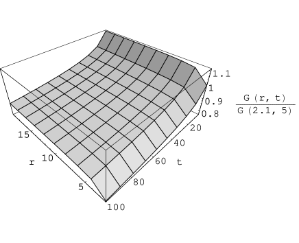
Figure 1: This graph illustrates the possible space and time variations that can arise in G in inhomogeneous solutions to the Brans–Dicke field equations, normalised at $r=2.1$ and $t=5$.

3.2 An Inhomogeneous Brans-Dicke Solution With Matter

We now seek a solution of the Brans-Dicke field equations (2) with the form

$$ds^{2}=e^{\nu}dt^{2}-e^{\mu}a^{2}(dr^{2}+r^{2}d\theta^{2}+r^{2}\sin^{2}\theta d\phi^{2})$$ (23)

where $e^{\nu}=e^{\nu(r)}$, $e^{\mu}=e^{\mu(r)}$ and $a=a(t)$. In Appendix A we show that a solution of the field equations (2) for a metric of the form (23) is given by

$$e^{\nu}=\left(\frac{1-\frac{c}{2kr}}{1+\frac{c}{2kr}}\right)^{2k},$$ (24)

$$e^{\mu}=\left(1+\frac{c}{2kr}\right)^{4}\left(\frac{1-\frac{c}{2kr}}{1+\frac{c}{2kr}}\right)^{2(k-1)(k+2)/k},$$ (25)

$$a(t)=a_{0}\left(\frac{t}{t_{0}}\right)^{\frac{2\omega(2-\gamma)+2}{3\omega\gamma(2-\gamma)+4}},$$ (26)

and

$$\phi(r,t)=\phi_{0}\left(\frac{t}{t_{0}}\right)^{\frac{2(4-3\gamma)}{3\omega\gamma(2-\gamma)+4}}\left(\frac{1-\frac{c}{2kr}}{1+\frac{c}{2kr}}\right)^{-2(k^{2}-1)/k}$$ (27)

for the matter distribution

$$\rho(r,t)=\rho_{0}\left(\frac{a_{0}}{a(t)}\right)^{3\gamma}\left(\frac{1-\frac{c}{2kr}}{1+\frac{c}{2kr}}\right)^{-2k}$$ (28)

where $k=\sqrt{\frac{4+2\omega}{3+2\omega}}$. This separable solution displays the same time dependence as the power–law FRW Brans-Dicke universes, (10)–(11), but with an additional inhomogeneous $r$–dependence created by the matter source at $r=0$. Such a distribution of matter in space is illustrated by figure 2. Here we have chosen, for illustrative purposes, $\gamma=1$, $\omega=100$ and a background value set by the choice $\rho=\rho_{FRW}$ ($\rho_{FRW}$ being the matter density that would be expected in the corresponding homogeneous universe). The temporal evolution of $\rho$ is exactly the same as the FRW case.

Figure 2: Distribution of $\rho$ as a function of $r$, with $\omega=100$, from eq. (28) and ${{\mathit{c=0.5}}}$.

We see from Figure 2 that the matter density is isotropic and asymptotically constant as $r\rightarrow\infty$ with a sharp power-law peak near the origin. Now (27) gives us

$$G(r,t)=G_{0}\left(\frac{1-\frac{c}{2kr}}{1+\frac{c}{2kr}}\right)^{2(k^{2}-1)/k}t^{-\frac{2(4-3\gamma)}{3\omega\gamma(2-\gamma)+4}}.$$ (29)

Equation (29) is used, with the values $\omega=100$, $\gamma=1$ and $c$ $=0.5$ to create Figure 3, which shows the space–time evolution of $G(r,t)$.

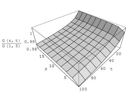
Figure 3: Evolution of $G(r,t)$ in space and time in an inhomogeneous matter dominated Universe, with $\omega=100$, from eq. (29) and $c=0.5.$

These results show how $G(r,t)$ can vary in space and time in an asymptotically–flat universe with a peak of matter at the origin. Observers located near the mass concentration will determine different values of $G$ locally although they will find the same values of $\dot{G}/G$ everywhere because of the separable nature of the $G(r,t)$ evolution in eq. (28). This was also the case for solution (22) given in subsection 3.2. In the next section we shall consider a more realistic model in which both $G$ and $\dot{G}/G$ are different from place to place. Plots like Figure 3 can be generated for universes dominated by other types of cosmological fluid and with different rates of density fall off with $r$.

4 Matching Two Vacuum FRW Brans-Dicke Universes

We will now consider a simple model of a spherically symmetric cosmological inhomogeneity produced by matching together flat and positively curved vacuum FRW–BD universes. This is a well studied technique, first introduced by Lemaître, for studying the non-linear evolution of overdensities in general relativistic FRW universes. The overdense region is modelled as a closed universe that at first expands more slowly than the background, before reaching an expansion  maximum and collapsing back to high density, whilst the background continues to expand. In this section we consider vacuum universes only, so there exists spherically symmetric inhomogeneity in the expansion rate and in $\phi\sim G^{-1},$ but $\rho=p=0$.

For flat vacuum FRW universes eq. (6) gives

$$\left(\frac{\dot{a}}{a}\right)^{2}+\frac{\dot{a}}{a}\frac{\dot{\phi_{b}}}{\phi_{b}}=\frac{\omega}{6}\left(\frac{\dot{\phi_{b}}}{\phi_{b}}\right)^{2}$$ (30)

where $\dot{}=\frac{d}{dt}$ and $\phi_{b}=\phi_{b}(t)$ is the BD scalar field and $a$ is the scale factor in the flat background. For a positively curved ($k=+1$) region the scale factor is taken to be $S(\tau)$, which satisfies the Friedmann equation for the closed vacuum BD universe:

$$\left(\frac{S^{\prime}}{S}\right)^{2}+\frac{S^{\prime}}{S}\frac{\phi_{p}^{\prime}}{\phi_{p}}=\frac{\omega}{6}\left(\frac{\phi_{p}^{\prime}}{\phi_{p}}\right)^{2}-\frac{k}{S^{2}},$$ (31)

where ${}^{\prime}=\frac{d}{d\tau}$, $\phi_{p}=\phi_{p}(\tau)$ and $\tau$ and $k$ are the proper time and curvature of this perturbed region.

In matching these two regions at $t=t_{0}=\tau_{0}$ we must satisfy the boundary conditions

$$S(\tau_{0}) =a(t_{0}), \left(\frac{dS}{d\tau}\right)_{0} =\left(\frac{da}{dt}\right)_{0},$$

$$\phi_{p}(\tau_{0}) =\phi_{b}(t_{0}) \text{and}\quad\left(\frac{d\phi_{p}}{d\tau}\right)_{0} =\left(\frac{d\phi_{b}}{dt}\right)_{0}.$$

4.1 The Background Universe

Assuming solutions of the form $\phi_{b}\propto t^{x}$ and $a\propto t^{y}$ and setting $a(0)=0$ gives, on substitution into (30) and (5), the $k=0$ BD vacuum solutions (O’Hanlon & Tupper, 1972)

$$a(t)=t^{\frac{1}{3}(1+2(1-\sqrt{3(3+2\omega)})^{-1})}$$ (32)

and

$$\phi_{b}(t)=\phi_{b0}\left(\frac{t}{t_{0}}\right)^{-2(1-\sqrt{3(3+2\omega)})^{-1}}.$$

4.2 A Collapsing Universe

For the closed region we now follow the method given in refs. (Barrow, 1992; Barrow & Parsons, 1997) to find expressions for $S(\tau)$ and $\phi_{p}(\tau)$. We start by introducing conformal time, $\eta$, defined by $Sd\eta=d\tau$; then eq. (5) becomes

$$\phi_{p},_{\eta\eta}+\frac{2}{S}S,_{\eta}\phi_{p},_{\eta}=0.$$

This integrates directly to yield

$$\phi_{p},_{\eta}S^{2}=\sqrt{3}A(2\omega+3)^{-1/2}$$ (33)

where $A$ is a constant. We now introduce the variable $y=\phi_{p}S^{2}$ to write (6) as

$$y,_{\eta}^{2}=-4ky^{2}+\frac{1}{3}\phi_{p},_{\eta}^{2}S^{4}(2\omega+3).$$ (34)

Now, eqs. (33) and (34) give

$$\frac{\phi_{p},_{\eta}}{\phi_{p}}=\sqrt{3}Ay^{-1}(2\omega+3)^{-1/2}$$

and

$$y,_{\eta}^{2}=-4ky^{2}+A^{2}.$$ (35)

The solutions of eqs. (35), when $k>0$, are given by

$$y(\eta)=\frac{A}{2\sqrt{k}}\sin(2\sqrt{k}(\eta+B),$$ (36)

and

$$\phi_{p}(\eta)=C\tan^{\sqrt{\frac{3}{(2\omega+3)}}}(\sqrt{k}(\eta+B))$$ (37)

where $B$ and $C$ are arbitrary constants. We now fix the conformal time origin by setting $B=0$, so that $y=\phi_{p}S^{2}$ gives

$$S(\eta)\propto\frac{\sin^{1/2}(2\sqrt{k}\eta)}{\tan^{\sqrt{\frac{3}{4(2\omega+3)}}}(\sqrt{k}\eta)}.$$ (38)

4.3 From $\eta$ to $t$

The function $\tau(\eta)$ is now obtained by integrating $Sd\eta=d\tau$ and $\tau(\eta)$ can then be used to obtain $S(\tau)$. We now require a relation between $t$ and $\tau$, for this we proceed as in ref. (Barrow & Kunze, 1997) and use the equation of relativistic hydrostatic equilibrium (Harrison, 1970, 1973), (Landau & Lifshitz, 1975)

$$\frac{\partial\Phi}{\partial r}=-\frac{\partial p/\partial r}{p+\rho}$$ (39)

where $\Phi$ is the Newtonian gravitational potential and $r$ is radial distance. Eqn. (39) is derived under the assumptions that the configuration is static and the gravitational field is weak, so $\Phi$ completely determines the metric; then (39) is given by the conservation of energy-momentum for a perfect fluid. We now use $d\tau=e^{\Phi}dt$, and for a scalar field we have an effective state with $p=\rho$ and $\rho=\frac{\omega}{\phi}\dot{\phi}^{2}$. Combining these results gives

$$\frac{d\tau}{dt}=\frac{\dot{\phi_{b}}}{\phi_{p}^{\prime}}\frac{\phi_{p}^{1/2}}{\phi_{b}^{1/2}}.$$ (40)

Now $\dot{\phi}_{b}\propto a^{-3}$ and $\phi_{p}^{\prime}\propto S^{-3}$, and so with (37) and (32) this gives

$$\frac{d\tau}{dt}=\frac{\sin^{1/2}(2\sqrt{k}\eta)}{\sin^{1/2}(2\sqrt{k}\eta_{0})}\frac{S^{2}}{S_{0}^{2}}\frac{a^{\sqrt{1+\frac{2}{3}\omega}-4}}{a_{0}^{\sqrt{1+\frac{2}{3}\omega}-4}}$$ (41)

Eq. (41) and the relation $Sd\eta=d\tau$ allow us to obtain $S(t)$ from (38). This is done numerically. Now fixing the constants of proportionality together with $k$ in eqs. (38), (37) and (32), in order to satisfy the boundary conditions, we find equations for the evolution of the scale factors and scalar fields in the flat background and perturbed region. These are matched at a boundary, at time $t_{0}=\tau_{0}=\eta_{0}$.

4.4 Results

Figure 4 shows the evolution of $a(t)$ and $S(t)$ when the region described by $S(t)$ becomes positively curved at initial time $t_{0}=1$. In Figure 4 we choose $\omega=100$, for illustrative purposes, and $a_{0}=S_{0}=1$ so that the boundary condition for the matching of the first derivatives of the scale factors is given by $\left(\frac{dS}{d\tau}\right)_{0}=\left(\frac{dS}{d\eta}\right)_{0}=\left(\frac{da}{dt}\right)_{0}.$

Figure 4: Evolution of the scale factor $S$ in the perturbed overdense region (dashed line) and in the background $a$(solid line) with respect to the comoving proper time in the flat background.

We can now express $G=G(t)$ in the regions of different curvature using equations (47), (37) and (32), along with the appropriate coordinate transformations. This gives Figure 5, below. It is clearly seen that the evolution of $G(t)$ is quite different in the two regions, as expected. The collapsing overdensity evolves faster than the background and possesses a smaller value of $G$ but a larger value of $|\dot{G}/G|\$at all times after the evolution commences.

Figure 5: Evolution of $G(t)$ in the overdense perturbed overdense region of positive curvature (dashed line) and in the spatially flat background universe (solid line).

5 A More Refined Spherical Collapse Model

We now generalise the spherical collapse model described in the last section to the more astronomically realistic case of a flat universe containing matter and a cosmological constant (see. e.g. refs. (Padmanabhan, 1995), (Peacock, 1999) or (Lahav et al., 1991)). As before, we match a flat Brans-Dicke FRW background to a spherically symmetric overdensity at an appropriate boundary and allow the two regions to evolve separately.

5.1 The background universe

Again, we consider a flat $(k=0)$, homogeneous and isotropic background universe. Since we are interested in the matter-dominated epoch, when structure formation starts, we can assume that our universe contains only matter and a vacuum energy contribution so that $\rho=\rho_{m}+\rho_{\Lambda}$ and $p=p_{\Lambda}=-\rho_{\Lambda}$ give the total density and pressure, respectively. So, for the flat background, eq. (6) gives for a general $\omega(\phi)$ theory,

$$\left(\frac{\dot{a}}{a}\right)^{2}+\frac{\dot{a}}{a}\frac{\dot{\phi}}{\phi}=\frac{\omega}{6}\frac{\dot{\phi}^{2}}{\phi^{2}}+\frac{8\pi}{3\phi}(\rho_{m}+\rho_{\Lambda})$$ (42)

and eq. (5) gives

$$\ddot{\phi}+3\frac{\dot{a}}{a}\dot{\phi}=\frac{8\pi}{(2\omega+3)}(\rho_{m}+4\rho_{\Lambda})-\frac{\dot{\omega}\dot{\phi}}{(2\omega+3)}.$$ (43)

Here, $\rho_{m}\propto a(t)^{-3}$ and $\rho_{\Lambda}=\text{constant}$. These equations govern the evolution of $\phi(t)$ and $a(t)$ in the flat expanding cosmological background. The contribution of the vacuum energy stress ($p=-\rho$) to the Friedmann equation (42) in BD cosmology differs from that in general relativity because of the presence of the variable $\phi$ field: it is not the same as the addition of a cosmological constant term to the RHS of (42). However, with this proviso, we shall continue to refer to $\Lambda$cdm models in Brans-Dicke theories in the following sections.

5.2 The overdensity

Again, we consider a spherical overdense region of radius $S$ and model the interior space-time as a closed FRW Brans-Dicke theory universe, ignoring any anisotropic effects of gravitational instability or collapse. As usual, we assume there is no shell-crossing; this implies mass conservation inside the overdensity and independence of the radial coordinate (Padmanabhan, 1995). The evolution equations can now be written in a form that ignores the spatial dependence of the fields. Put $\rho=\rho_{cdm}+\rho_{\Lambda}$ and $p=p_{\Lambda}=-\rho_{\Lambda}$, where ’cdm’ corresponds to cold dark matter, so that (8) gives

$$\ddot{S}-\dot{S}\frac{\dot{\phi_{c}}}{\phi_{c}}=-S\left(\frac{\omega_{c}}{3}\frac{\dot{\phi_{c}}^{2}}{\phi_{c}^{2}}-\frac{1}{2}\frac{\dot{\omega}_{c}}{(2\omega_{c}+3)}\frac{\dot{\phi}_{c}}{\phi_{c}}\right.\\ \left.+\frac{8\pi}{3\phi_{c}}\frac{(\rho_{cdm}(3+\omega_{c})+\rho_{\Lambda}(3-2\omega_{c}))}{(2\omega_{c}+3)}\right)$$ (44)

while (5) reduces to

$$\ddot{\phi_{c}}+3\frac{\dot{S}}{S}\dot{\phi_{c}}=\frac{8\pi}{(2\omega_{c}+3)}(\rho_{cdm}+4\rho_{\Lambda})-\frac{\dot{\omega_{c}}\dot{\phi_{c}}}{(2\omega_{c}+3)}$$ (45)

where $S=S(t)$ is the scale factor and $\phi_{c}=\phi_{c}(t)$ is the BD scalar field in the collapsing region of positive curvature where $\rho_{cdm}\propto S(t)^{-3}$ and $\rho_{\Lambda}=\text{constant}$. These equations give the evolution of $\phi_{c}(t)$ and $S(t)$.

We have assumed that the equation of motion of the field inside the cluster overdensity is described by the local space-time geometry. This means that the field follows the dark-matter collapse from the beginning of the cluster’s formation. We do not consider this to be fully realistic since there is expected to be an outflow of energy associated with $\phi$ from the overdensity to the background universe, as first noticed by Mota and van de Bruck (Mota & van de Bruck (2004)). The details of this outflow of energy and its effect on the collapse can only be determined by a fully relativistic hydrodynamical calculation, which is beyond the scope of this study. Nevertheless, at late times during the collapse of the dark matter (and especially when the density contrast in the dark matter is very large) the field should no longer feel the effects of the expanding background and will decouple from it. We are also neglecting the effects of deviations from spherical symmetry, which grow during the collapse in the absence of pressure, along with rotation, gravitational tidal interactions between different overdensities, and all forms of non-linear hydrodynamical complexity.

5.3 Evolution of the overdensity

Consider the spherical perturbation in the cdm fluid with a spatially constant internal density. Initially, this perturbation is assumed to have a density amplitude $\delta_{i}>0$ where $|\delta_{i}|\ll 1$. The initial cdm density inside the overdensity is therefore $\rho_{cdm}=\rho_{m}(1+\delta_{i})$.

Four characteristic phases of the overdensity’s evolution can be identified:

• Expansion: we employ the initial boundary condition $\phi_{c}=\phi$ and assume that at early times the overdensity expands along with the background.

• Turnaround: for a sufficiently large $\delta_{i},$ gravity prevents the overdensity from expanding forever; the spherical overdensity breaks away from the general expansion and reaches a maximum radius. Turnaround is defined as the time when $S=S_{max}$, $\dot{S}=0$ and $\ddot{S}<0$.

• Collapse: the overdensity subsequently collapses ($\dot{S}<0$). If pressure and dissipative physics are ignored the overdensity would collapse to a singularity where the density of matter would tend to infinity. In reality this singularity does not occur; instead, the kinetic energy of collapse is transformed into random motions.

• Virialisation: dynamical equilibrium is reached and the system becomes stationary with a fixed radius and constant energy density.

We require our spherical overdensity to evolve from the linear perturbation regime at high redshift until it becomes non-linear, collapses, and virialises. Thereafter, the overdensity will become gravitationally stable and further local evolution of the scale factor and of the scalar field will cease. However, the background scale factor will continue to expand, and so the background density and background value of $G$ will continue to decrease. As a result, a significant disparity between the evolution of $G$ inside and outside the cluster can result.

5.4 Virialisation

In scalar-tensor theories we expect that the gravitational potential will not be of the standard local $r^{-1}$ form. This requires reconsideration of the virial condition. According to the virial theorem, equilibrium will be reached when (Goldstein, 1980)

$$T=\frac{1}{2}S\frac{\partial U}{\partial S}$$ (46)

where $T$ is the average total kinetic energy, $U$ is the average total potential energy and $S$ here denotes the radius of the spherical overdensity.

The potential energy for a given component $x$ can be calculated from its general form in a spherical region (Landau & Lifshitz, 1975)

$$U_{x}=2\pi\int_{0}^{S}\rho_{tot}\Phi_{x}r^{2}dr,$$

where $\rho_{tot}$ is the total energy density and $\Phi_{x}$ is the gravitational potential due to the density component $\rho_{x}$.

The gravitational potential $\Phi_{x}$ can be obtained from the weak-field limit of the field equations (2). This results in a Poisson equation where the terms associated to the scalar field can be absorbed into the definition of the Newtonian constant as (Will, 1993)

$$G_{c}=\frac{4+2\omega_{c}(\phi_{c})}{3+2\omega_{c}(\phi_{c})}\frac{1}{\phi_{c}}.$$ (47)

This results in the usual form for the Newtonian potential

$$\Phi_{x}\left(s\right)=-2\pi G_{c}\rho_{x}(3\gamma_{x}-2)\left(S^{2}-\frac{r^{2}}{3}\right)$$

where $G_{c}$ is given by equation (47) and $\gamma_{x}-1$ is $p_{x}/\rho_{x}$ for the fluid component with density $\rho_{x}$ and pressure $p_{x}$ (appearing due to the relativistic correction to Poisson’s equation: $\Delta\Phi=4\pi G\left(\rho+3p\right)$).

In $\Lambda$cdm models of structure formation it is entirely plausible to set $\gamma_{x}=1$ as the energy density of the cosmological constant is negligible on the virialised scales we are considering (Wang & Steinhardt, 1998; Mota & van de Bruck, 2004). The potential energies associated with a given component ($x$) inside the overdensity are now given by

$$U_{x}=-\frac{16\pi^{2}}{15}G_{c}\rho_{tot}\rho_{x}S^{5}.$$ (48)

Therefore, the virial theorem will be satisfied when

$$T_{vir}=\frac{1}{2}S_{vir}\left(\frac{\partial U}{\partial S}\right)_{vir},$$

where

$$\frac{\partial U}{\partial S}=-\frac{16\pi^{2}}{15}\left[\frac{\partial G_{c}}{\partial S}\rho_{tot}\rho_{x}S^{5}+\right.\\ \left.G_{c}\frac{\partial\rho_{tot}}{\partial S}\rho_{x}S^{5}+G_{c}\rho_{tot}\frac{\partial\rho_{x}}{\partial S}S^{5}+G_{c}\rho_{tot}\rho_{x}5S^{4}\right]$$ (49)

and we have used $U_{tot}=U_{cdm}+U_{\Lambda}+U_{\phi_{c}}$, $\rho_{tot}=\rho_{cdm}+\rho_{\Lambda}+\rho_{\phi_{c}}$, $\rho_{\phi_{c}}=\omega_{c}\dot{\phi}^{2}/\phi$ and

$$\frac{\partial G_{c}}{\partial S}=\frac{\dot{G}_{c}}{\dot{S}}=-G_{c}\ \dot{\phi}_{c}\frac{3+2\omega_{c}}{4+2\omega_{c}}\left(G_{c}+\frac{2\omega_{c}^{{}^{\prime}}(\phi_{c})}{(3+2\omega_{c})^{2}}\right).$$

The other components of eq. (49) are obtained from eqs. (44) and (45).

Using eq. (46), together with energy conservation at turnaround and virialisation, we obtain an equilibrium condition in terms of potential energies only

$$\frac{1}{2}S_{vir}\left(\frac{\partial U}{\partial S}\right)_{z_{v}}+U_{tot}(z_{v})=U_{tot}(z_{ta}),$$ (50)

where $z_{v}$ is the redshift at virialisation and $z_{ta}$ is the redshift of the over-density at its turnaround radius. The behaviour of $G$ during the evolution of an overdensity can now be obtained by numerically evolving the background eq. (42)-(43) and the overdensity eqs. (44) and (45) until the virial condition (50) holds.

We point out here an inconsistency when one makes use of equation (50) together with the assumption that energy is not conserved. This inconsistency is removed by assuming a negligible outflow of $\phi$ from the overdensity, in which case we regain energy conservation within the system and so retain self-consistency.

5.5 Overdensities vs Background

5.5.1 Brans–Dicke theory

 

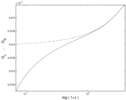
(a) $\omega=40000$

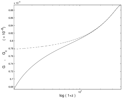
(b) $\omega=500$

Figure 6: Plots of $G$ against $\ln(1+z)$ in the background (dashed-line) and in an overdensity (solid-line), for different values of $\omega.$ Initial conditions are chosen in both cases so as to give $G=G_{0}$, the present value of the Newton constant, at virialisation. We note that increasing $\omega$ decreases the difference in $G$ between the overdensity and the background.

The Brans–Dicke coupling parameter $\omega$ is constant and constrained by a variety of local gravitational tests (see (Uzan, 2003) for a review). The strongest constraint to date is derived from observations of the Shapiro time delay of signals from the Cassini space craft as it passes behind the Sun. These considerations led Bertotti, Iess and Tortora (Bertotti, Iess & Tortora, 2003), after a complicated data analysis process, to claim that $\omega$ must have a value greater than $40000$ (to $2\sigma$). This limit on $\omega$ must be satisfied at all times in all parts of the universe, and leads to the conclusion that Brans-Dicke theory must be phenomenologically very similar to general relativity throughout most of the history of the universe. However, we do still expect a cosmological evolution of the Brans-Dicke field $\phi$ which determines the value of Newton’s $G$; and we expect this evolution to be different in regions that collapse to form the structure probed by Cassini compared to that in the idealised expanding cosmological background, as described above. Hence we expect the measurable value of $G$ to be different in these two distinct regions with different histories. It is quite possible that the region of gravitational equilibrium probed by Cassini and other local observations would find no perceptible change in $G$ locally despite the presence of change on cosmological scales outside of bound inhomogeneities.

In this section we quantify this difference in $G$ by numerically evolving $a$, $S$, $\phi$ and $\phi_{c}$ until virialisation occurs. At virialisation, the evolution of $S$ and $\phi_{c}$ is expected to end, giving a value of $G$ that is locally constant in time even though the cosmological evolution of $a$ and $\phi$ continues.

The plots in figure 6 were constructed using the representative values $\omega=40000$ and $\omega=500$ and the boundary condition $\phi_{c0}\simeq G_{0}^{-1}$, so that the value of $G$ measured inside the overdensity at present is equal to the value of Newton’s $G$, as measured locally. The evolution of the background was determined by matching $\phi_{c}$ to $\phi$ at the time when the overdensity decouples from the background, $t_{i}$. We see a clear difference in the evolution of $G$ in the two regions, as expected. This example shows that we expect different values of $G$ and $\dot{G}/G$ inside and outside virialised overdensities. The present value of $G$ and $\dot{G}/G$ depends on the history of the region where it was sampled, as well as on the Brans–Dicke coupling parameter, $\omega$.

It can be seen from the plots in figure 6 that increasing $\omega$ has the effect of decreasing the difference in $G$ between the background universe and the overdensity. The size of this inhomogeneity is found to be of order $1/\omega$ and, correspondingly, reduces to zero as $\omega\rightarrow\infty$. This is an important consistency check for the methods used as we expect Brans–Dicke theory to reduce to general relativity, with a constant $G$, in this limit.

5.5.2 Scalar-tensor theory with $2\omega+3=2A\left|1-\frac{\phi}{\phi_{\infty}}\right|^{-p}$

 

(a) $2\omega(\phi)+3$ for p=2 and A=1, 2 and 5 (solid, dashed and dotted lines, respectively).

(b) $2\omega(\phi)+3$ for A=1 and p=1.5, 2 and 2.5 (solid, dashed and dotted lines, respectively).

Figure 7: In these gravity theories there is fast approach to general relativity at late times when $\phi\rightarrow\phi_{\infty}$, but significantly different behaviour at early times.

Next, we consider a scalar–tensor theory with a variable $\omega(\phi)$. We investigate the class of theories defined by the choice of coupling function

$$2\omega(\phi)+3=2A\left|1-\frac{\phi}{\phi_{\infty}}\right|^{-p},$$

where $A$, $\phi_{\infty}$, and $p$ are positive definite constants. We refer to this as Theory 1. Such a choice of coupling was considered by Barrow and Parsons and was solved exactly for the case of a flat FRW universe containing a perfect fluid (Barrow & Parsons, 1997).

Setting the constants as $2A=\left(\phi_{\infty}/\beta\right)^{2}$ and $p=2$ gives us the scalar–tensor theory considered by Damour and Pichon (Damour & Pichon, 1999) and by Santiago, Kalligas and Wagoner (Santiago, Kalligas & Wagoner, 1997). This choice of $\omega(\phi)$ corresponds to setting $\ln A(\phi)=\ln A(\phi_{0})+\frac{1}{2}\beta(\phi_{\infty}-\phi)^{2}$, where $A^{2}(\phi)$ is the conformal factor $1/\phi$ from eq. (12). Damour and Nordvedt (Damour & Nordvedt, 1993) consider this function as a potential and therefore justify its choice in relation to the generic parabolic form near a potential minimum. Expecting the function to be close to zero (i.e. GR), Santiago, Kalligas and Wagoner justify its expression as a perturbative expansion. This choice of $\omega(\phi)$ with $p>1/2$ corresponds to a general two–parameter class of scalar–tensor theories that are close to GR and will be drawn ever closer to it with $\omega\rightarrow\infty$ and $\omega^{\prime}/\omega^{3}\rightarrow 0$ as the universe expands and $\phi\rightarrow\phi_{\infty}$. We therefore consider it as a representative example of a wide family of plausible varying-$G$ theories that generalise Brans-Dicke.

The evolution of this form of $\omega(\phi)$ is shown graphically in figure 7 for different values of $A$ and $p$. Clearly the evolution of $\omega(\phi)$ is sensitive to both $A$ and $p$ and so the choice of these parameters is important for the form of the underlying theory. For illustrative purposes we choose here the values $p=1.5,2$ and $5$ and $A=1,2$ and $5$.

In a similar way to the BD case we now create an evolution of $\phi_{c}$ that virialises at $z=0$ to give the value $G_{c0}=6.673\times 10^{-11}$, as observed experimentally. The corresponding evolution for $\phi_{b}$ is calculated as before by matching it to the value of $\phi_{c}$ at the time the overdensity decouples from the background and begins to collapse. In creating these plots we have used the conservative parameter values $p=2$, $\omega_{c0}=1.2\times 10^{5}$ and $A=6\times 10^{-7}$ which are consistent with observation and allow structure formation to occur in a similar way to general relativity. The results of this are plotted in figure 8.

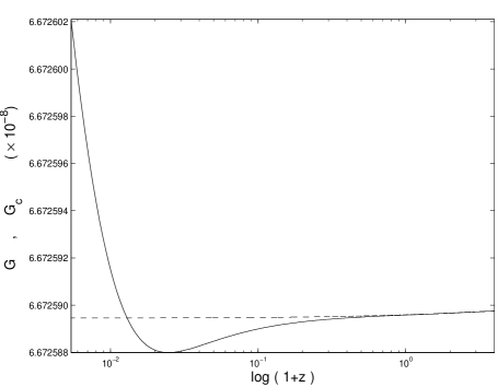
Figure 8: $2\omega+3=2A\left|1-\frac{\phi}{\phi_{\infty}}\right|^{-2}$ A graph of   the variation $G$ against $\ln(1+z)$ for the background universe (dashed-line) and inside an overdensity (solid-line) which give $G=G_{0},$the presently observed terrestrial value, at virialisation.

Again, we note the different evolution of $G(t)$ in the two regions, and the difference in the asymptotic values of $G$. We note that experimental measurements of $G$ on Earth have a significant uncertainty with the 1998 CODATA value carrying an uncertainty 12 times greater than the standard value adopted in 1987. The 1998 value is given as (Mohr & Taylor, 2000; Scherrer, 1999)

$$G_{1998}=6.673\pm 0.010\times 10^{-8}cm^{3}gm^{-1}s^{-2},$$

while the 2002 CODATA pre-publication announcement reverts to the earlier higher accuracy consensus with (National Institute of Standards and Technology, 2002)

$$G_{2002}=6.6742\pm 0.0010\times 10^{-8}cm^{3}gm^{-1}s^{-2}\$$

We could re–run the above analysis with different values of $A$ and $p$, but expect that the results would look qualitatively similar. From Figure 7 we see that increasing (decreasing) the values of $A$ and $p$ will increase (decrease) the value of $\omega(\phi)$ for a given $\phi$, thereby making the theory more (less) like GR. We therefore expect an analysis with a higher (lower) value of $A$ and/or $p$ to look very similar to the analysis presented above with a less (more) rapid evolution of $G(t)$. For the sake of brevity we omit such an analysis here.  

5.6 Space and Time variations of $G$

We now calculate how time and space variations of $G$ evolve with redshift and depend on the cdm density contrast, $\Delta_{c}$. In order to do this, we make the definitions

$$\frac{\Delta G}{G}(t)\equiv\frac{G(t)-G_{0}}{G_{0}},\qquad\frac{\delta G}{G}(t)\equiv\frac{G_{c}(t)-G_{b}(t)}{G_{b}(t)}$$

and

$$\Delta_{c}\equiv\frac{\rho_{cdm}(z_{v})}{\rho_{m}(z_{v})},$$

where $G_{c}$ and $G_{b}$ correspond to $G$ as measured in the overdensity and in the background universe respectively.

The results of our numerical calculations, for a cluster which virialises at $z_{v}=0$, are presented in Figures 9, 10 and 11, respectively. These plots display the evolution of $\dot{G}/G,\Delta G/G,$ and $\delta G/G$ with redshift for Brans-Dicke, the theory of subsection 5.5.2, and some other choices of $\omega(\phi)$ that are specified in the captions. The parameters used in generating these plots are $B=0.4$, $C=10^{-16}$, $D=80$, $A=6\times 10^{-7}$, $p=2$ and $\omega=4\times 10^{6}$. These values were chosen so as to agree with observation and so that structure formation is not significantly different from that which occurs in general relativity.

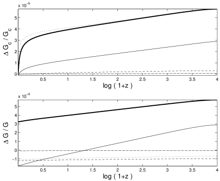
Figure 9: Evolution of $\Delta G/G$ as a function of $log(1+z)$ for overdensities which virialise at $z=0$ in a $\Lambda$cdm model. Upper plot: evolution inside the overdensity. Lower plot: evolution in the background universe. Thick solid line $2\omega+3=4\times 10^{6}$, thin solid line $2\omega+3=B^{2}\phi$, dashed-line $2\omega+3=2A|1-\frac{\phi}{\phi_{0}}|^{-2}$, dash-dotted line $2\omega+3=C|\ln(\frac{\phi}{\phi_{0}})|^{-4}$, dotted line $2\omega+3=D|1-(\frac{\phi}{\phi_{0}})^{2}|^{-1}$ . Each model is normalised in order to have $G_{0}=G_{c}(z=0)$ inside the overdensities.

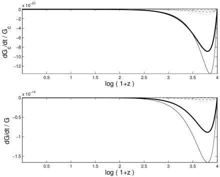
Figure 10: Evolution of $\dot{G}/G$ as a function of $log(1+z)$ for overdensities which virialise at $z=0$ in a $\Lambda$cdm model. Upper plot: evolution inside the overdensity. Lower plot: evolution in the background universe. Thick solid line $2\omega+3=4\times 10^{6}$, thin solid line $2\omega+3=B^{2}\phi$, dashed-line $2\omega+3=2A|1-\frac{\phi}{\phi_{0}}|^{-2}$, dash-dotted line $2\omega+3=C|\ln(\frac{\phi}{\phi_{0}})|^{-4}$, dotted line $2\omega+3=D|1-(\frac{\phi}{\phi_{0}})^{2}|^{-1}$ . Each model is normalised in order to have $G_{0}=G_{c}(z=0)$ inside the overdensities.

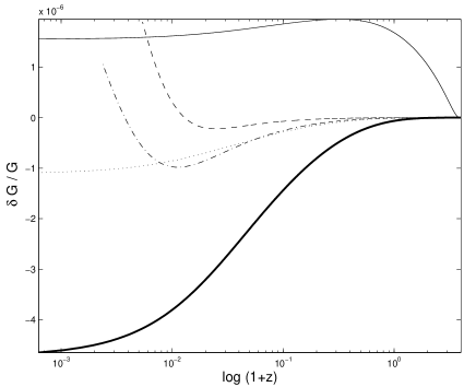
Figure 11: Evolution of $\delta G/G$ as a function of $log(1+z)$ for overdensities which virialise at $z=0$ in a $\Lambda$cdm model. Thick solid line $2\omega+3=4\times 10^{6}$, thin solid line $2\omega+3=B^{2}\phi^{2(p+1)}$, dashed-line $2\omega+3=2A|1-\frac{\phi}{\phi_{0}}|^{-2}$, dash-dotted line $2\omega+3=C|\ln(\frac{\phi}{\phi_{0}})|^{-4}$, dotted line $2\omega+3=D|1-(\frac{\phi}{\phi_{0}})^{2}|^{-1}$ . Each model is normalised in order to have $G_{0}=G_{c}(z=0)$ inside the overdensities.

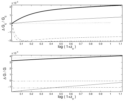
Figure 12: Values of $\Delta G/G$ as a function of $log(1+z_{v})$ at virialisation. Upper plot: evolution inside the overdensity. Lower plot: evolution in the background universe. Thick solid line $2\omega+3=4\times 10^{6}$; thin solid line $2\omega+3=B^{2}\phi$; dashed-line $2\omega+3=2A|1-\frac{\phi}{\phi_{0}}|^{-2}$; dash-dotted line $2\omega+3=C|\ln(\frac{\phi}{\phi_{0}})|^{-4}$; dotted line $2\omega+3=D|1-(\frac{\phi}{\phi_{0}})^{2}|^{-1}$ . Each model is normalised to have $G_{0}=G_{c}(z=0)$ inside the overdensities.

It is clear from the plots that different scalar-tensor theories lead to different variations of $G$. The predictions of these models can be quite diverse. While some models produce higher values of $G$ inside the overdensity, others produce a lower one. A feature common to all models is that the value of $G$ and $\dot{G}/G$ inside an overdensity is different from $G$ and $\dot{G}/G$ in the background universe. The reason for these differences is that in the non–linear regime, when the overdensity decouples from the background expansion at turnaround, the field $\phi$ that drives variations in the Newtonian gravitational “constant” stops feeling the background expansion. After turnaround, the field inside the overdensity, $\phi_{c}$, deviates from the field, $\phi$, in the background universe, leading to spatial variations in $G$. In reality, such spatial inhomogeneities in the value of $G$ are small: $\delta G/G\approx 10^{-6}$, Figure 11. The time variations of $G$ are even smaller than the spatial inhomogeneities but with a marked difference between the inside and outside rates of change. We find $\dot{G}_{c}/G_{c}\leq 10^{-20}s^{-1}$ inside the clusters and $\dot{G}/G\leq 10^{-19}s^{-1}$ in the background, Figure 10.

Figures 12, 13 and 14 represent the values of $\Delta G/G$, $\delta G/G$ and $\dot{G}/G$ at the redshift of virialisation ($z_{v}$). Once again the differences between the different scalar-tensor theories and between $G_{c}(z_{v})$ and $G(z_{v})$ are evident.

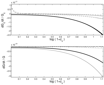
Figure 13: Values of $\dot{G}/G$ as a function of $log(1+z_{v})$ at virialisation. Upper plot: evolution inside the overdensity. Lower plot: evolution in the background universe. Thick solid line $2\omega+3=4\times 10^{6}$; thin solid line $2\omega+3=B^{2}\phi$; dashed-line $2\omega+3=2A|1-\frac{\phi}{\phi_{0}}|^{-2}$; dash-dotted line $2\omega+3=C|\ln(\frac{\phi}{\phi_{0}})|^{-4}$; dotted line $2\omega+3=D|1-(\frac{\phi}{\phi_{0}})^{2}|^{-1}$. Each model is normalised to have $G_{0}=G_{c}(z=0)$ inside the overdensities.

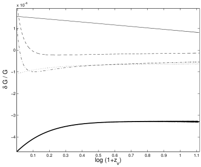
Figure 14: Values of $\delta G/G$ as a function of $log(1+z_{v})$ at virialisation. Thick solid line $2\omega+3=4\times 10^{6}$; thin solid line $2\omega+3=B^{2}\phi$; dashed-line $2\omega+3=2A|1-\frac{\phi}{\phi_{0}}|^{-2}$; dash-dotted line $2\omega+3=C|\ln(\frac{\phi}{\phi_{0}})|^{-4}$; dotted line $2\omega+3=D|1-(\frac{\phi}{\phi_{0}})^{2}|^{-1}$. Each model is normalised to have $G_{0}=G_{c}(z=0)$ inside the overdensities.

Figure 15 shows how the cdm contrast, $\Delta_{c}\equiv\rho_{cdm}(z_{v})/\rho_{m}(z_{v})$, affects the difference between the value of $G$ inside an overdensity and in the cosmological background. (Recall that, in the Einstein–de Sitter model $\Delta_{\mathrm{c}}\equiv\rho_{cdm}(z_{v})/\rho_{m}(z_{v})\approx 147$ at virialisation, and $\Delta_{\mathrm{c}}\equiv\rho_{cdm}(z_{v})/\rho_{m}(z_{c})\approx 187$ at collapse). It is interesting to see that different scalar-tensor theories produce a different dependence.

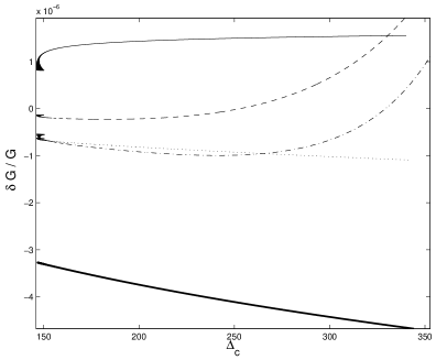
Figure 15: Values of $\delta G/G$ as a function of $\Delta_{c}$ for a $\Lambda$cdm model. Thick-solid line $2\omega+3=4\times 10^{6}$; solid line $2\omega+3=B^{2}\phi$; dashed-line $2\omega+3=2A|1-\frac{\phi}{\phi_{0}}|^{-2}$; dash-dotted line $2\omega+3=C|\ln(\frac{\phi}{\phi_{0}})|^{-4}$; dotted line $2\omega+3=D|1-(\frac{\phi}{\phi_{0}})^{2}|^{-1}$. Each model is normalised to have $G_{0}=G_{c}(z=0)$ inside the overdensities.

From the numerical simulations, we see that a variation of the Newtonian gravitational constant, of the order presented here, does not affect the predictions of the structure formation models. For instance, the virialisation radius and the density contrast $\Delta_{c}$ of the virialised clusters are very similar to the $\Lambda$cdm and standard cdm models with constant $G$ . Nevertheless, one should point out that different scalar-tensor theories lead to slightly different results. Besides that, there is also a dependence on the initial conditions, as with many other cosmological scalar fields (see e.g. (Mota & van de Bruck, 2004; Mota & Barrow, 2004a, b)). Different initial conditions will lead to slightly different allowed values of $\omega$ and to different cosmological behaviours of $G$ and $G_{c}$.

6 Conclusions

We have studied the inhomogeneous cosmological evolution of the Newtonian gravitational ’constant’ $G$ within the framework of relativistic scalar-tensor theories of gravity, of which Brans–Dicke theory is the simplest and best known case. We began by first exploiting the conformal equivalence between these theories and general relativity to transform an existing solution of Einstein’s field equations to a new exact spherically symmetric inhomogeneous vacuum cosmological solution of the Brans–Dicke field equations. We then present a second spherically symmetric perfect-fluid solution to the Brans–Dicke field equations which corresponds to an overdense inhomogeneity in an asymptotically homogenous and isotropic expanding cosmological background. These exact solutions have simple enough form to allow the $G(r,t)$ evolution to be investigated directly and can be used to model the presence of a Schwarzschild-like mass in an expanding Brans–Dicke universe that approaches an idealised FRW universe asymptotically as $r\rightarrow\infty$. It is noted that far from the mass $G$ varies very slowly with $r$ and that as $r\rightarrow\infty$ the variation of $G$ with $r$ is removed altogether and only the cosmological evolution of $G$ with time is relevant. Close to the mass, the $r$ variation of $G$ becomes more significant and we see that $G$ $\rightarrow 0$ at small $r$. We also note that in the limit $\omega\rightarrow\infty$ all space and time variation in $G$ is removed from these solutions and general relativity is recovered.

Next, we increased the complexity of the model by matching together two vacuum FRW–Brans–Dicke universes of zero and positive curvature on a spacelike time slice. This results in a simple model for a spherically symmetric perturbation in the density and curvature that is followed into the non–linear regime. The different evolutions of $G$ in the two regions were determined and a comparison was made of the different evolutions of $G$ on spacelike slices of differing time. We see from this toy model that the value of $G$ does indeed have a different value in regions that have decoupled from the expanding cosmological background and collapsed, compared to its value in the background itself. We were then able to repeat this construction for a more realistic matching of two FRW $\Lambda$cdm universes of different curvature in an arbitrary scalar–tensor gravity theory. We followed the development of spherical overdensities through their expansion, separation from the background, turnaround, and subsequent collapse. Applying a simple approximation to virialise the collapsing overdensities, we were then able to study the differences in $G(\vec{x},t)$ between the non-expanding overdensity and the expanding background universe. We highlight as a special case the simple Brans–Dicke theory but also present results for other scalar–tensor gravity theories, specified by their defining coupling function $\omega(\phi)$. Although each theory predicts a different detailed cosmological evolution of $G$, a feature common to all of them is the sharp difference between the value and time evolution of $G$ inside bound overdensities and in the background universe. These differences will produce spatial inhomogeneities in $G$ with a value which depends on the scalar–tensor theory used. While some models produce higher values of $G$ inside the overdensity, others produce a lower one. In spite of these differences, such spatial inhomogeneities are small $\delta G/G\approx 10^{-6}$. The differences in the time variations of $G$ were found, with typically $\dot{G}_{c}/G_{c}\leq 10^{-20}s^{-1}$ inside the clusters and $\dot{G}/G\leq 10^{-19}s^{-1}$ in the background universe in the range of theories studied. Such variations in $G$ do not significantly alter the virialisation radius and the density contrast $\Delta_{c}$ of the virialised clusters from those in standard $\Lambda$cdm and cdm models with constant $G$. Nevertheless, different scalar-tensor theories lead to slightly different results. There is also a dependence on the initial conditions. Different initial conditions will lead to a different value of $\omega$ and to different cosmological behaviours of $G$ and $G_{c}$. Taken as a whole these analyses show that local observational limits on varying $G$ made within our solar system or Galaxy must be used with caution when placing constraints upon the allowed cosmological variation of $G$ on extragalactic scales or in the early universe. The universe is not spatially homogeneous and, in cosmological models where it can vary, nor is $G$.

ACKNOWLEDGEMENTS
We would like to thank Andrew Liddle for helpful comments and suggestions. DFM is supported by Fundacão Ciência e a Tecnologia. TC is supported by the PPARC.

Appendix A Inhomogeneous field equations

Substituting (23) into (2) gives, for a perfect fluid

$$\frac{8\pi}{\phi}p=-\left[2\frac{\ddot{a}}{a}+\left(\frac{\dot{a}}{a}\right)^{2}+\frac{\omega}{2}\left(\frac{\dot{\phi}}{\phi}\right)^{2}+2\frac{\dot{a}}{a}\frac{\dot{\phi}}{\phi}+\frac{\ddot{\phi}}{\phi}\right]e^{-\nu}\\ +\left[\frac{\mu^{{\prime}^{2}}}{4}+\frac{\mu^{\prime}\nu^{\prime}}{r}+\frac{\mu^{\prime}\nu^{\prime}}{2}-\frac{\omega}{2}\left(\frac{\phi^{\prime}}{\phi}\right)^{2}\right.\\ \left.+\frac{\phi^{\prime}}{\phi}\left(\mu^{\prime}+\frac{\nu^{\prime}}{2}+\frac{2}{r}\right)\right]e^{-\mu}a^{-2},$$ (51)

$$\frac{8\pi}{\phi}p=-\left[2\frac{\ddot{a}}{a}+\left(\frac{\dot{a}}{a}\right)^{2}+\frac{\omega}{2}\left(\frac{\dot{\phi}}{\phi}\right)^{2}+2\frac{\dot{a}}{a}\frac{\dot{\phi}}{\phi}+\frac{\ddot{\phi}}{\phi}\right]e^{-\nu}\\ +\left[\frac{\mu^{\prime\prime}\nu^{\prime\prime}}{2}+\frac{\nu^{{\prime}^{2}}}{4}+\frac{\mu^{\prime}+\nu^{\prime}}{2r}+\frac{\omega}{2}\left(\frac{\phi^{\prime}}{\phi}\right)^{2}+\right.\\ \left.\frac{\phi^{\prime\prime}}{\phi}+\left(\frac{\nu^{\prime}}{2}+\frac{1}{r}\right)\frac{\phi^{\prime}}{\phi}\right]e^{-\mu}a^{-2},$$ (52)

and

$$-\frac{8\pi}{\phi}\rho=-\left[3\left(\frac{\dot{a}}{a}\right)^{2}-\frac{\omega}{2}\left(\frac{\dot{\phi}}{\phi}\right)^{2}+3\frac{\dot{a}}{a}\frac{\dot{\phi}}{\phi}\right]e^{-\nu}\\ +\left[\mu^{\prime\prime}+\frac{\mu^{{\prime}^{2}}}{4}+\frac{2\mu^{\prime}}{r}+\frac{\omega}{2}\left(\frac{\phi^{\prime}}{\phi}\right)^{2}\right.\\ \left.+\frac{\phi^{\prime\prime}}{\phi}+\left(\frac{\nu^{\prime}}{2}+\frac{1}{r}\right)\frac{\phi^{\prime}}{\phi}\right]e^{-\mu}a^{-2}$$ (53)

as the $T^{11}$, $T^{22}$ and $T^{00}$ equations, respectively. The propagation equation (3) now becomes

$$\frac{8\pi(\rho-3p)}{(2\omega+3)\phi}=\left[\frac{\ddot{\phi}}{\phi}+3\frac{\dot{a}}{a}\frac{\dot{\phi}}{\phi}\right]e^{-\nu}\\ -\left[\frac{\phi^{\prime\prime}}{\phi}+\frac{(\mu^{\prime}+\nu^{\prime})}{2}\frac{\phi^{\prime}}{\phi}+\frac{2}{r}\frac{\phi^{\prime}}{\phi}\right]e^{-\mu}a^{-2}.$$ (54)

and the only other non-trivial field equation is that for $T^{10}$;

$$\nu^{\prime}\frac{\dot{a}}{a}-\omega\frac{\dot{\phi}}{\phi}\frac{\phi^{\prime}}{\phi}-\frac{\dot{\phi}^{\prime}}{\phi}+\frac{\dot{a}}{a}\frac{\phi^{\prime}}{\phi}+\frac{\nu^{\prime}}{2}\frac{\dot{\phi}}{\phi}=0.$$ (55)

We now assume $\phi$ is of the form $\phi(r,t)=\phi(r)\phi(t)$ and look for solutions to the set of equations

$$\frac{\mu^{{\prime}^{2}}}{4}+\frac{\mu^{\prime}\nu^{\prime}}{r}+\frac{\mu^{\prime}\nu^{\prime}}{2}\\ =\frac{\omega(r)}{2}\left(\frac{\phi^{\prime}(r)}{\phi(r)}\right)^{2}-\frac{\phi^{\prime}(r)}{\phi(r)}\left(\mu^{\prime}+\frac{\nu^{\prime}}{2}+\frac{2}{r}\right),$$ (56)

$$\frac{\mu^{\prime\prime}\nu^{\prime\prime}}{2}+\frac{\nu^{{\prime}^{2}}}{4}+\frac{\mu^{\prime}+\nu^{\prime}}{2r}\\ =-\frac{\omega}{2}\left(\frac{\phi^{\prime}(r)}{\phi(r)}\right)^{2}-\frac{\phi^{\prime\prime}(r)}{\phi(r)}-\left(\frac{\nu^{\prime}}{2}+\frac{1}{r}\right)\frac{\phi^{\prime}(r)}{\phi(r)},$$ (57)

$$\mu^{\prime\prime}+\frac{\mu^{{\prime}^{2}}}{4}+\frac{2\mu^{\prime}}{r}\\ =-\frac{\omega}{2}\left(\frac{\phi^{\prime}(r)}{\phi(r)}\right)^{2}-\frac{\phi^{\prime\prime}(r)}{\phi(r)}-\left(\frac{\nu^{\prime}}{2}+\frac{1}{r}\right)\frac{\phi^{\prime}(r)}{\phi(r)},$$ (58)

and

$$\frac{\phi^{\prime\prime}(r)}{\phi(r)}+\frac{(\mu^{\prime}+\nu^{\prime})}{2}\frac{\phi^{\prime}(r)}{\phi(r)}+\frac{2}{r}\frac{\phi^{\prime}(r)}{\phi(r)}=0.$$ (59)

Such solutions are given by (Nariai, 1969) as

$$e^{\nu}=\left(\frac{1-\frac{c}{2kr}}{1+\frac{c}{2kr}}\right)^{2k},$$ (60)

$$e^{\mu}=\left(1+\frac{c}{2kr}\right)^{4}\left(\frac{1-\frac{c}{2kr}}{1+\frac{c}{2kr}}\right)^{2(k-1)(k+2)/k},$$ (61)

and

$$\phi(r)=\phi_{0}\left(\frac{1-\frac{c}{2kr}}{1+\frac{c}{2kr}}\right)^{-2(k^{2}-1)/k}$$ (62)

where $k=\sqrt{\frac{4+2\omega}{3+2\omega}}$. For $e^{\nu}$ and $e^{\mu}$ of this form, equations (51), (53) and (54) become

$$\frac{8\pi(\rho e^{\nu}-3pe^{\nu})}{(2\omega+3)\phi(t)}=\frac{\ddot{\phi(t)}}{\phi(t)}+3\frac{\dot{a}}{a}\frac{\dot{\phi(t)}}{\phi(t)},$$ (63)

$$\frac{8\pi}{\phi(t)}\rho e^{\nu}=3\left(\frac{\dot{a}}{a}\right)^{2}-\frac{\omega}{2}\left(\frac{\dot{\phi(t)}}{\phi(t)}\right)^{2}+3\frac{\dot{a}}{a}\frac{\dot{\phi(t)}}{\phi(t)},$$ (64)

and

$$-\frac{8\pi}{3\phi(t)}\frac{(3\omega pe^{\nu}+3\rho e^{\nu}+\omega\rho e^{\nu})}{(2\omega+3)}\\ =\frac{\ddot{a}}{a}-\frac{\dot{a}}{a}\frac{\dot{\phi(t)}}{\phi(t)}+\frac{\omega}{3}\left(\frac{\dot{\phi(t)}}{\phi(t)}\right)^{2}.$$ (65)

Where (65) was obtained by substituting (51) and (53) into (54) and discarding the terms involving $r$ derivatives, as these now sum to zero. We see that (63), (64) and (65) are simply (4), (5) and (6) with $k=0$, $p_{FRW}=pe^{\nu}$ and $\rho_{FRW}=\rho e^{\nu}$, where subscript _FRW denotes a quantity derived from the field equations using the FRW metric. We also have, from $T_{;\nu}^{\mu\nu}=0$, that

$$\frac{d}{dt}(\rho e^{\nu})+3H(\rho e^{\nu}+pe^{\nu})=0.$$ (66)

Looking for solutions of the form $a\propto t^{x}$ and $\phi(t)\propto t^{y}$ gives, on substitution into (63), the relation $y=2-3x\gamma$ (assuming an equation of state for the Universe of the form $p=(\gamma-1)\rho$). Using (63), (64), and this relation then gives the solutions

$$a(t)=a_{0}\left(\frac{t}{t_{0}}\right)^{\frac{2\omega(2-\gamma)+2}{3\omega\gamma(2-\gamma)+4}},$$ (67)

and

$$\phi(t)=\phi_{0}\left(\frac{t}{t_{0}}\right)^{\frac{2(4-3\gamma)}{3\omega\gamma(2-\gamma)+4}}.$$ (68)

These are exactly the same as would be expected for the scale factor and the BD field in a flat FRW Universe (Nariai, 1968). The form of $\rho$ is then given by (66) and (60) as

$$\rho(r,t)=\rho_{0}\left(\frac{a_{0}}{a(t)}\right)^{3\gamma}\left(\frac{1-\frac{c}{2kr}}{1+\frac{c}{2kr}}\right)^{-2k},$$ (69)

and $\phi(r,t)$ is given as

$$\phi(r,t)=\phi_{0}\left(\frac{t}{t_{0}}\right)^{\frac{2(4-3\gamma)}{3\omega\gamma(2-\gamma)+4}}\left(\frac{1-\frac{c}{2kr}}{1+\frac{c}{2kr}}\right)^{-2(k^{2}-1)/k}.$$ (70)

References

- Barrow (1992) Barrow J.D., 1992, Phys. Rev. D 47, 5329
- Barrow & Kunze (1997) Barrow J.D., Kunze C. 1997, Phys. Rev. D, 57, 2255
- Barrow & O’Toole (2001) Barrow J.D., O’Toole C. 2001, Mon. Not. Roy. Astron. Soc. 322, 585
- Barrow & Parsons (1997) Barrow J.D., Parsons P. 1997, Phys. Rev. D, 55, 1906
- Bertotti, Iess & Tortora (2003) Bertotti B., Iess L., Tortora P. , 2003, Nature 425, 374
- Brans & Dicke (1961) Brans C., Dicke R., 1961, Phys. Rev. 124. 925
- Bergmann (1968) Bergmann P.G. 1968, Int. J. Theo. Phys. 1, 25
- Capozziello et al. (1996) Capozziello S., De Ritis R., Rubano C. , Scudellaro P., 1996, Int. J. Mod. Phys. D 5, 85
- Cervantes-Cota & Nahmad (2001) Cervantes-Cota J.L., Nahmad M., 2001, Gen. Rel. Grav. 33, 767
- Damour & Nordvedt (1993) Damour T. , Nordvedt K., 1993, Phys. Rev. D 48, 3436
- Damour & Pichon (1999) Damour T. , Pichon B., 1999, Phys. Rev. D 59, 123502
- Fuji & Maeda (2003) Fuji Y., Maeda K.I., 2003 The Scalar-Tensor Theory of Gravitation (Cambridge University Press, Cambridge).
- Garcia-Bellido, Linde & Linde (1994) Garcia-Bellido J., Linde A., Linde D., 1994, D. Phys. Rev. D 50, 730
- Goldstein (1980) Goldstein H., 1980, Classical Mechanics, 2nd edn. (Addison-Wesley, Reading, Mass)
- Green, Schwartz & Witten (1987) Green M., Schwartz. J., Witten E., 1987, Superstring Theory (Cambridge University Press, Cambridge).
- Gurevich, Finkelstein & Ruban (1973) Gurevich L.E., Finkelstein A.M., Ruban V.A., 1973, Astrophys. Sp. Sci. 22, 231
- Harrison (1970) Harrison E.R. , 1970, Phys. Rev. D, 1, 2726
- Harrison (1973) Harrison E.R. , 1973, in Cargèse Lectures in Physics, Vol. 6, ed. E. Schatzmann, Gordon and Breach, NY
- Holden & Wands (1998) Holden D.J., Wands D., 1998, Class. Quant. Grav. 15, 3271
- Husain, Martinez & Nunez (1994) Husain V., Martinez E.A., Nunez D., 1994,Phys. Rev. D, 50, 3783
- Jordan (1949) Jordan P., 1949, Nature 164, 637
- Jordan (1955) Jordan P., 1955, Schwerkraft und Weltall (Vieweg, Baunschweig )
- Jordan (1959) Jordan P., 1959, Z. Phys. 157, 112
- Lahav et al. (1991) Lahav O., et al., 1991, Mon. Not. Roy. Astron. Soc. 251, 128
- Landau & Lifshitz (1975) Landau L.D., Lifshitz E.M., 1975, Classical Theory of Fields, 4th edn., (Pergamon, Oxford).
- Mohr & Taylor (2000) Mohr P.J., Taylor B., 2000, Rev. Mod. Phys. 72, 351
- Mota & Barrow (2004a) Mota D.F., Barrow J.D., 2004a, Mon. Not. Roy. Astron. Soc. 349:281
- Mota & Barrow (2004b) Mota D.F., Barrow J.D., 2004b, Phys. Lett. B 581 141
- Mota & van de Bruck (2004) Mota D.F., van de Bruck C., 2004, Astron. & Astrophys. in press, astro-ph/0401504.
- National Institute of Standards and Technology (2002) National Institute of Standards and Technology, 2002, www.physics.nist.gov/cuu/Constants
- Nariai (1968) Nariai H., 1968, Prog. Theo. Phys., 40, 49
- Nariai (1969) Nariai H., 1969, Prog. Theo. Phys., 42, 742
- Nordtvedt (1970) Nordtvedt K., 1970, Ap. J. 161, 1059
- O’Hanlon & Tupper (1972) O’Hanlon J., Tupper B.O., 1972, Nuovo Cim. 7, 305
- Ohashi, Tagoshi & Sasaki (1996) Ohashi A., Tagoshi H., Sasaki M., 1996, Prog. Theor. Phys. 96, 713
- Padmanabhan (1995) Padmanabhan T., 1995, Structure formation in the universe, (Cambridge University Press, Cambridge)
- Peacock (1999) Peacock J., 1999, Cosmological Physics, (Cambridge University Press, Cambridge)
- Pimentel (1997) Pimentel L.O., 1997, Mod. Phys. Lett. A 12, 1865
- Riazi & Ahmadi-Azar (1995) Riazi N., Ahmadi-Azar E., 1995, Astrophys. Space Sci. 226, 1
- Santiago, Kalligas & Wagoner (1997) Santiago D., Kalligas D., Wagoner R.V. , 1997, Phys. Rev. D 56, 7627
- Scheel, Shapiro & Teukolsky (1995) Scheel M.A., Shapiro S.L., Teukolsky S.A., 1995, Phys. Rev. D 51, 4208
- Scherrer (1999) Scherrer R.J., astro-ph/0310699
- Tamaki, Maeda & Torii (1999) Tamaki T., Maeda K., Torii T., 1999, Phys. Rev. D 60, 104049
- Uzan (2003) Uzan J.P., 2003, Rev. Mod. Phys. 75, 403
- Wagoner (1970) Wagoner R.V., 1970, Phys. Rev. D 1, 3209
- Wang & Steinhardt (1998) Wang L.M., Steinhardt P.J., 1998, Astrophys. J. 508, 483
- Will (1993) Will C.M., 1993, Theory and Experiment in Gravitational Physics, 2nd edn. (Cambridge University Press, Cambridge).