Asymptotic Analysis of Field Commutators for Einstein-Rosen Gravitational Waves

Abstract

We give a detailed study of the asymptotic behavior of field commutators for linearly polarized, cylindrically symmetric gravitational waves in different physically relevant regimes. We also discuss the necessary mathematical tools to carry out our analysis. Field commutators are used here to analyze microcausality, in particular the smearing of light cones owing to quantum effects. We discuss in detail several issues related to the semiclassical limit of quantum gravity, in the simplified setting of the cylindrical symmetry reduction considered here. We show, for example, that the small G behavior is not uniform in the sense that its functional form depends on the causal relationship between spacetime points. We consider several physical issues relevant for this type of models such as the emergence of large gravitational effects.

I Introduction

Among the many symmetry reductions of General Relativity that have been considered in the past, linearly polarized cylindrical waves (also known as Einstein-Rosen waves Einstein and Rosen (1937); Kuchar (1971)) have been the focus of intensive study. They provide a model with an infinite number of degrees of freedom that can be exactly solved in spite of the fact that it is non-linear. This is not only true classically but also quantum mechanically, and hence this system is a valuable tool to explore the physics that may be found if a successful quantization of full general relativity is ever achieved Ashtekar and Pierri (1996); Ashtekar (1996); Angulo and Mena Marugan (2000); Barbero G. et al. (2003).

One of the main reasons behind this success is the fact that the physical Hamiltonian is a function of the free Hamiltonian of a 2+1 dimensional, axially symmetric, massless scalar field evolving in an auxiliary Minkowskian background Ashtekar (1996); Angulo and Mena Marugan (2000); Ashtekar et al. (1997). In a previous paper Barbero G. et al. (2003) we took advantage of this fact to study the quantum corrections to the spacetime structure by considering the commutator of this scalar field at different spacetime points. As is well known, microcausality in quantum field theories can be discussed by looking at the commutator of quantum fields (or anticommutator in the case of fermions). In the standard examples the microcausality requirement means that this (anti)commutator must vanish for spatially separated spacetime points. A similar argument can be made for vector fields, though issues of gauge invariance change some of the conclusions; in particular if one computes the commutator of the four-vector potential $A_{\mu}$ at two spatially separated points, it may be different from zero in some gauges, even though it is always true that the commutator of gauge invariant objects is zero for such points.

The issue of gauge invariance in the context of cylindrical gravitational waves has been discussed at length by Bičák and collaborators Kouletsis et al. (2003). These authors show that is is legitimate to use the Ashtekar-Pierri gauge fixed action Ashtekar and Pierri (1996) written in terms of the scalar field that encodes the physical information in this model to obtain gauge invariant structures such as Dirac observables or the S matrix. This justifies the computation of the type of objects –field commutators– that we will be considering here to extract conclusions about the quantum structure of spacetime.

The particular problem that we will be concerned with in this paper is the detailed study of the field commutator (given as a certain integral) and, in particular, its limiting behavior when the time and length separations are much larger than the natural length scale of the problem –the Planck length–. In order to do this the procedure of expanding the integrand of the field commutator as a power series in the gravitational constant and other asymptotic parameters is not useful. In fact it will be necessary to adapt some methods developed for the asymptotic analysis of integrals and get a consistent procedure to expand the relevant objects as asymptotic series. It is possible to understand this a posteriori as a consequence of the fact that some limiting behaviors (i.e. in $G$) of the field commutator change in a non trivial way as the spacetime intervals go from spacelike to timelike or when one of the spacetime points lies in the symmetry axis. Also the functional dependence in some of these parameters is highly non-polynomial. This is not what one would expect to obtain in the familiar perturbative treatment of quantum field theories (QFT’s).

The paper is divided in two main sections: a physical discussion of the behavior of the field commutator followed by a detailed description of the asymptotic methods necessary to study the different physically relevant regimes. Specifically, after this introduction we will give the different asymptotic expansions for all the relevant parameters (involving the $G\rightarrow 0$ limit and also the limits in which the difference in the time coordinates or the radial coordinates go to infinity). Using them we will discuss the main physical consequences of the quantization of this model as far as microcausality is concerned. In this respect it is particulary interesting to point out the existence of a certain type of large quantum mechanical effects (in a sense that will be made precise later) when one of the spacetime points in the field commutator lies in the symmetry axis.

A technical issue that should be considered is the role of regulators in the final physical results. As is well known regulators are necessary to give sense to otherwise ill-defined objects. They must be introduced, for example, to obtain a finite norm vector by acting with the field operator on the vacuum state. Cut-offs are a simple way to regulate amplitudes. It is conceivable that physical regulators exist that restrict, for example, the integration intervals for some physical objects (such as the field commutators considered here) to finite real intervals. However it is also possible that they are just a convenient way to render some physical objects finite in such a way that no footprint is left in the final results. This is the philosophy that one has in mind in the usual renormalization scheme where cut-offs are taken to infinity and disappear from physical quantities.

The point of view of this paper is that the un-regulated objects (integrals), when defined, are a good approximation to the regulated ones. The asymptotic analysis of regulated commutators and their relation with the un-regulated ones will be discussed elsewhere.

In the usual perturbative QFT computations Green functions, matrix elements, and similar objects are expanded as power series in the coupling constants of the model with coefficients that are usually written as regulated integrals. This is a necessary step because it is usually not possible to write them in closed form. Here the situation is different because it is possible to write down expressions for the objects of interest (field commutators in the present example) that depend on the coupling constants in a non trivial way. This has the advantage of allowing us to use approximation techniques specially adapted to their specific form and much better suited to its study. It also permits to consider some problems that may be difficult to tackle for the usual QFT’s; for example one can try to figure out if the asymptotic behavior of some regulated object coincides with its asymptotic behavior after the regulator is removed.

A detailed technical discussion of the techniques needed to explore the relevant asymptotic regimes is presented in section III. These techniques will be useful tools in order to analyze other types of physical objects (such as S-matrix elements) so they provide the necessary background for a perturbative framework properly adapted to this model, this is why we invest some time to study them here. We end the paper with a summary of the main results, comments, perspectives for future work, and several appendices. Numerical and algebraic computations have been performed with the aid of Mathematica$\textregistered$.

II The field commutator

We start with a brief description of the model and introduce our conventions and notation. As is well known Romano and Torre (1996); Kuchar (1971); Einstein and Rosen (1937) Einstein-Rosen waves correspond to topologically trivial spacetimes with two linearly independent, commuting, spacelike, and hypersurface orthogonal Killing vector fields. The metric in this case can be writen as

$$ds^{2}=e^{\gamma-\psi}(-dT^{2}+dR^{2})+e^{-\psi}R^{2}d\theta^{2}+e^{\psi}dZ^{2},$$ (1)

where we are using coordinates $(T,R,\theta,Z),\,\,T\in\mathbb{R},\,\,R\in[0,\infty),\,\,\theta\in[0,2\pi),\,\,Z\in\mathbb{R}$, and $\psi$ and $\gamma$ are functions only of $R$ and $T$. The Einstein field equations for this metric are very simple: the scalar field $\psi$ must satisfy the wave equation for a massless, axially symmetric scalar field in three dimensions

$$\partial_{T}^{2}\psi-\partial_{R}^{2}\psi-\frac{1}{R}\partial_{R}\psi=0$$

and the function $\gamma$ can be expressed in terms of this field on the classical solutions Ashtekar and Pierri (1996); Angulo and Mena Marugan (2000) as

$$\gamma(R)=\frac{1}{2}\int^{R}_{0}d\bar{R}\,\bar{R}\,\left[(\partial_{T}\psi)^{2}+(\partial_{\bar{R}}\psi)^{2}\right].$$

Throughout the paper we will use a system of units such that $c=\hbar=1$ and define $G\equiv\hbar G_{3}$, where $G_{3}$ denotes the gravitational constant per unit length in the direction of the symmetry axis. The metric function $\gamma(R)$ admits a simple physical interpretation: apart from a factor of $8G$ it is the energy of the scalar field in a ball of radius $R$, and $\gamma_{\infty}\equiv\lim_{R\rightarrow\infty}\gamma(R)$ the energy of the whole two-dimensional flat space. Furthermore, $\gamma_{\infty}/8G$ coincides with the Hamiltonian $H_{0}$ of the system obtained by linearizing the metric (1)Ashtekar and Pierri (1996); Barbero G. et al. (2003).

In order to arrive at a unit asymptotic timelike Killing vector that allows us to introduce a physical notion of energy (per unit length) it is convenient to use coordinates $(t,R,\theta,Z)$ defined by $T=e^{-\gamma_{\infty}/2}t$. In these coordinates the metric takes the form Kuchar (1971); Romano and Torre (1996)

$$ds^{2}=e^{\gamma-\psi}(-e^{-\gamma_{\infty}}dt^{2}+dR^{2})+e^{-\psi}R^{2}d\theta^{2}+e^{\psi}dZ^{2}.$$

By choosing a metric function $\psi$ with a sufficiently fast fall-off as $R\rightarrow\infty$, this metric describes asymptotically flat spacetimes with a certain (non-zero) deficit angle and such that $\partial_{t}$ is a unit timelike Killing vector in the asymptotic region.

The Einstein field equations can be obtained from a Hamiltonian action principle Ashtekar and Varadarajan (1994); Varadarajan (1995); Romano and Torre (1996) where the Hamiltonian $H$ is a function of that corresponding to the free scalar field, $H_{0}$:

$$H=E(H_{0})=\frac{1}{4G}(1-e^{-4GH_{0}}).$$

In the following we will refer to $t$ as the physical time and to $H$ as the physical Hamiltonian.

In terms of the $T$-time and imposing that $\psi$ be regular at $R=0$ Ashtekar and Pierri (1996), the classical solutions for the field $\psi$ can be written as

$$\psi(R,T)=\sqrt{4G}\int_{0}^{\infty}\!\!dk\,J_{0}(Rk)\left[A(k)e^{-ikT}+A^{\dagger}(k)e^{ikT}\right]$$

where $A(k)$ [and its complex conjugate $A^{\dagger}(k)$] are determined by the initial conditions. The free Hamiltonian $H_{0}$ can be written now as

$$\gamma_{\infty}=H_{0}=\int_{0}^{\infty}dk\,kA^{\dagger}(k)A(k).$$

Using this expression, we can obtain the $t$-evolution of the field

$$\psi_{E}(R,t)=\sqrt{4G}\int_{0}^{\infty}\!\!dk\,J_{0}(Rk)\left[A(k)e^{-ikte^{-\gamma_{\infty}/2}}\!+\!A^{\dagger}(k)e^{ikte^{-\gamma_{\infty}/2}}\right].\;$$

The quantization can be carried out by following the usual steps. We introduce a Fock space in which $\hat{\psi}(R,0)$, the quantum counterpart of $\psi(R,0)$, is an operator-valued distribution Reed and Simon (1975). Its action is determined by those of $\hat{A}(k)$ and $\hat{A}^{\dagger}(k)$, the annihilation and creation operators with non-vanishing commutators given by

$$\left[\hat{A}(k_{1}),\hat{A}^{\dagger}(k_{2})\right]=\delta(k_{1},k_{2}).$$

Explicitly,

$$\hat{\psi}(R,0)\!=\!\hat{\psi}_{E}(R,0)\!=\!\sqrt{4G}\int_{0}^{\infty}\!\!\!dk\,J_{0}(Rk)\!\left[\hat{A}(k)\!+\!\hat{A}^{\dagger}(k)\right]\!.$$

Evolution in $T$ is given by the unitary operator $\hat{U}_{0}(T)=\exp(-iT\hat{H}_{0})$ where

$$\hat{H}_{0}=\int^{\infty}_{0}dk\,k\,\hat{A}^{\dagger}(k)\hat{A}(k)$$

is the quantum Hamiltonian operator of a three dimensional, axially symmetric scalar field. The quantum scalar field in the Heisenberg picture is hence given by

$$\hat{\psi}(R,T)=\hat{U}^{\dagger}_{0}(T)\hat{\psi}(R,0)\hat{U}_{0}(T)=\sqrt{4G}\int_{0}^{\infty}\!\!dk\,J_{0}(Rk)\!\left[\hat{A}(k)e^{-ikT}\!+\!\hat{A}^{\dagger}(k)e^{ikT}\right]\!.\hskip 8.5359pt$$

If we choose the physical time $t$ to define the evolution in our model, the quantum Hamiltonian is $\hat{H}=E(\hat{H}_{0})=\frac{1}{4G}(1-e^{-4G\hat{H}_{0}})$ and unitary evolution is given by $\hat{U}(t)=\exp(-it\hat{H})$. With this time evolution the annihilation and creation operators in the Heisenberg picture are

$$\hat{A}_{E}(k,t)\!\! \equiv \!\!\hat{U}^{\dagger}(t)\hat{A}(k)\hat{U}(t)=\exp\!\left[-itE(k)e^{-4G\hat{H}_{0}}\right]\!\hat{A}(k),$$

$$\hat{A}_{E}^{\dagger}(k,t)\!\! = \!\hat{A}^{\dagger}(k)\,\exp\!\left[itE(k)e^{-4G\hat{H}_{0}}\right],$$

where $E(k)=\frac{1}{4G}(1-e^{-4Gk})$, and the field operator evolved with the physical Hamiltonian [that we denote as $\hat{\psi}_{E}(R,t)$] is given by

$$\hat{\psi}_{E}(R,t)=\sqrt{4G}\int_{0}^{\infty}\!\!\!dk\,J_{0}(Rk)\left[\hat{A}_{E}(k,t)+\hat{A}_{E}^{\dagger}(k,t)\right].$$

The field commutator $\big{[}\hat{\psi}_{E}(R_{1},t_{1}),\hat{\psi}_{E}(R_{2},t_{2})\big{]}$ can be computed from these expressions Barbero G. et al. (2003). One of its interesting features is the fact that it is not proportional to the identity as in the case of free theories (or if we consider the quantum evolution defined by the Hamiltonian $H_{0}$ of the linearized model) but is a non-diagonal operator in the chosen basis. We are hence led to consider its matrix elements. We will concentrate here on the most relevant of these elements (at least from the perspective of the microcausality of the classical background of the model), namely the vacuum expectation value, which is explicitly given by

$$\frac{1}{8iG}\langle 0|\,[\hat{\psi}_{E}(R_{1},t_{1}),\hat{\psi}_{E}(R_{2},t_{2})]\,|0\rangle=\int_{0}^{\infty}\!\!\!\!\!\!dk\,J_{0}(R_{1}k)J_{0}(R_{2}k)\sin\left[\frac{t_{2}-t_{1}}{4G}(1\!-\!e^{-4Gk})\right]\!.\hskip 11.38092pt$$ (2)

As we can see it depends on the time coordinates through their difference $t_{2}-t_{1}$ (which we will assume to be, e.g., positive) and depends symmetrically on $R_{1}$ and $R_{2}$. The functional dependence in $G$ is less trivial, a fact that will require especial attention when studying the limit in which the relevant lengths and time differences are much larger than the Planck length. For comparison purposes we remember that

$$\frac{1}{8iG}\langle 0|\,[\hat{\psi}(R_{1},T_{1}),\hat{\psi}(R_{2},T_{2})]\,|0\rangle=\int_{0}^{\infty}\!\!\!\!\!\!dk\,J_{0}(R_{1}k)J_{0}(R_{2}k)\sin\left[k(T_{2}-T_{1})\right]\!.\hskip 11.38092pt$$ (3)

In the following it will be convenient to refer the dimensional parameters of the integral to another length scale that we choose as $R_{1}$. We hence define $R_{2}=\rho R_{1}$, $t_{2}-t_{1}=\tau R_{1}$, $\lambda=R_{1}/4G$ and rewrite (2) as

$$\frac{1}{8iG}\langle 0|\,[\hat{\psi}_{E}(R_{1},t_{1}),\hat{\psi}_{E}(R_{2},t_{2})]\,|0\rangle=\frac{\lambda}{R_{1}}\Im\bigg{\{}\int_{0}^{\infty}dqJ_{0}(\lambda q)J_{0}(\rho\lambda q)e^{i\tau\lambda(1-e^{-q})}\bigg{\}}$$ (4)

after introducing the new variable $k=q/4G$. Here $\Im$ denotes the imaginary part.

II.1 Asymptotic behavior in $\rho$: smearing of light cones

The integral (4) can be written as a standard $h$-transform Bleistein and Handelsman (1986), with asymptotic parameter $\rho$, by the change of variables $t=q\lambda$,

$$\frac{1}{R_{1}}\Im\bigg{\{}\int_{0}^{\infty}\!\!dt\,J_{0}(\rho t)J_{0}(t)e^{i\tau\lambda(1-e^{-t/\lambda})}\bigg{\}}.$$ (5)

In this case a straightforward Mellin transform analysis Bleistein and Handelsman (1986) (discussed in section III) gives the following asymptotic behavior in the $\rho\rightarrow\infty$ limit

$$\frac{1}{R_{1}}\Im\bigg{\{}\frac{1}{\rho}+\frac{1}{\rho^{3}}\Big{(}\frac{1}{4}+\frac{\tau^{2}}{2}+\frac{i\tau}{2\lambda}\Big{)}+\frac{9}{\rho^{5}}\Big{(}\frac{1}{64}-\frac{i\tau}{24\lambda^{3}}+\frac{i\tau}{8\lambda}+\frac{\tau^{2}}{8}+\frac{i\tau^{2}}{4\lambda}-\frac{7\tau^{2}}{24\lambda^{2}}+\frac{\tau^{4}}{24}\Big{)}+O\Big{[}\frac{1}{\rho^{7}}\Big{]}\bigg{\}}$$

$$=\frac{1}{R_{1}}\bigg{\{}\frac{\tau}{2\lambda\rho^{3}}+\frac{1}{\rho^{5}}\Big{(}\frac{9\tau}{8\lambda}-\frac{3\tau}{8\lambda^{3}}+\frac{9\tau^{2}}{4\lambda}\Big{)}+O\Big{[}\frac{1}{\rho^{7}}\Big{]}\bigg{\}}.$$ (6)

The asymptotic behavior in the $\rho\rightarrow\infty$ limit gives a precise and quantitative description of the smearing of (cylindrically symmetric) light cones because it shows, for example, that for fixed values of $R_{1}$ and $(t_{2}-t_{1})$ the expectation value of the commutator (over $8iG$) falls off for large values of $R_{2}$ as

$$\frac{2G(t_{2}-t_{1})}{R_{2}^{3}}+O\bigg{[}\frac{1}{R_{2}^{5}}\bigg{]}.$$

This means that even for large spatial separations the scalar field that encodes the gravitational field does not commute with itself.

In the $\rho\rightarrow 0^{+}$ limit, on the other hand, we get

$$\frac{1}{R_{1}}\Im\bigg{\{}\int_{0}^{\infty}dtJ_{0}(t)e^{i\tau\lambda(1-e^{-t/\lambda})}\bigg{\}}+O(\rho).$$ (7)

This shows that the commutator is a continuous function of $\rho$ in $\rho=0$, a fact that will be important in the analysis of the semiclassical limit.

II.2 Asymptotic behavior in $\tau$: large quantum gravity effects

The integral in (5) has the convenient form of a $h$-transform if the asymptotic parameter is chosen to be $\rho$; however this is no longer true if the asymptotic parameter is $\tau$ (which corresponds to considering large separations in the time coordinates). This introduces some mathematical difficulties in the asymptotic analysis that will be discussed later.

In this case one has to perform separate analyses for $\rho=0$ and $\rho\neq 0$. In $\rho=0$ one finds that the asymptotic behavior when $\tau\rightarrow\infty$ is given by

$$\frac{1}{R_{1}}\bigg{[}\frac{\lambda}{2\pi\log\tau}\bigg{]}^{1/2}\Im\bigg{\{}e^{i[\frac{\pi}{4}+\tau\lambda-\lambda\log(\tau\lambda)]}e^{\frac{\pi}{2}\lambda}\Gamma(i\lambda)+e^{-i[\frac{\pi}{4}-\tau\lambda-\lambda\log(\tau\lambda)]}e^{-\frac{\pi}{2}\lambda}\Gamma(-i\lambda)\bigg{\}}+O\bigg{[}\frac{1}{(\log\tau)^{3/2}}\bigg{]},$$ (8)

whereas for $\rho\neq 0$ we find

$$\frac{1}{2\pi R_{1}\sqrt{\rho}\log\tau}\times$$

$$\Im\bigg{\{}e^{i[\frac{\pi}{2}+\tau\lambda-\lambda(1+\rho)\log(\tau\lambda)]}e^{\frac{\pi}{2}\lambda(1+\rho)}\Gamma[i\lambda(1+\rho)]+e^{-i[\frac{\pi}{2}-\tau\lambda-\lambda(1+\rho)\log(\tau\lambda)]}e^{-\frac{\pi}{2}\lambda(1+\rho)}\Gamma[-i\lambda(1+\rho)]\hskip 17.07164pt$$ (9)

$$+e^{i[\tau\lambda-\lambda(1-\rho)\log(\tau\lambda)]}e^{\frac{\pi}{2}\lambda(1-\rho)}\Gamma[i\lambda(1-\rho)]+e^{i[\tau\lambda-\lambda(\rho-1)\log(\tau\lambda)]}e^{\frac{\pi}{2}\lambda(\rho-1)}\Gamma[i\lambda(\rho-1)]\bigg{\}}+O\bigg{[}\frac{1}{(\log\tau)^{2}}\bigg{]}.$$

The most striking feature of these expressions is the unusual dependence on the asymptotic parameter $\tau$; in fact the dependence on inverse powers of logarithms (especially on the inverse square root of $\log\tau$) cannot be obtained by direct application of the usual asymptotic expressions derived by Mellin transform techniques. It is also remarkable how slowly the commutator decays in $\tau$ –in particular in the axis $\rho=0$– a fact that is suggestive of the large quantum gravity effects discussed by Ashtekar in Ashtekar (1996). Outside the axis the decay is quicker but still rather slow. A consequence of the different asymptotic behaviors in $\tau$ for $\rho=0$ and $\rho\neq 0$ is the impossibility to recover (8) as the limit when $\rho\rightarrow 0$ of (9). It is interesting to point out that the frequency of the oscillations of the commutator in the $\tau$ parameter is controlled by the value of $\lambda$ (proportional to the inverse of $G$) in such a way that although the amplitude of the oscillations decays very slowly they will average to the value of the free commutator on scales much larger than the Planck length.

The $\tau\rightarrow 0$ limit is simpler to analyze. Actually we find that the series obtained by expanding $e^{i\tau\lambda(1-e^{-t/\lambda})}$ as a power series in $e^{-t/\lambda}$, exchanging integration and infinite sum, and computing the resulting integrals gives an expansion that converges to the value of the commutator.

II.3 Asymptotic behavior in $\lambda$: the semiclassical limit

The possibility of studying the asymptotic behaviors in $\rho$ and $\tau$ by using the powerful mathematical tools provided by the theory of Mellin transforms relies on the fact that these integrals can be written as $h$-transforms of the type mentioned above. However this is no longer possible if one wants to study the limit $\lambda\rightarrow\infty$ (corresponding to the situation when $R_{1}$ is much larger than the Planck length) because of the particular dependence of these integrals on $\lambda$. There is, however, a way out of this if one is willing to abandon Mellin transforms: writing the integral in (4) as a multiple integral by introducing the integral representation of the Bessel functions $J_{n}$ ($n=0,\,1,\,\ldots$),

$$J_{n}(z)=\frac{1}{2\pi i}\oint_{\gamma}\frac{dt}{t^{n+1}}e^{\frac{z}{2}(t-\frac{\scriptstyle 1}{\scriptstyle t})},$$

where $\gamma$ is a closed, positively oriented, simple path in the complex plane surrounding the origin. By doing this the right hand side (r.h.s.) of (4) can be rewritten in the following form

$$-\frac{1}{R_{1}}\Im\Big{\{}\frac{\lambda e^{i\tau\lambda}}{4\pi^{2}}\int_{0}^{\infty}dq\oint_{\gamma_{1}}dt_{1}\oint_{\gamma_{2}}dt_{2}\frac{1}{t_{1}t_{2}}e^{\lambda\big{[}\frac{\scriptstyle q}{\scriptstyle 2}(t_{1}-\frac{\scriptstyle 1}{\scriptstyle t_{1}})+\frac{\scriptstyle\rho q}{\scriptstyle 2}(t_{2}-\frac{\scriptstyle 1}{\scriptstyle t_{2}})-i\tau e^{-q}\big{]}}\Big{\}}.$$ (10)

Although the contours $\gamma_{1}$ and $\gamma_{2}$ may be different in principle we will take them equal in practice. Besides, we will see in the next section that it is convenient to choose them in a specific way.

As in the $\tau$ case one has to perform separate asymptotic analyses for $\rho=0$ and $\rho\neq 0$. In order to proceed it is necessary to divide the $(\rho,\,\tau)$ plane into the same regions that appear in the discussion of the “free” commutator (3) which corresponds to the evolution dictated by the Hamiltonian $H_{0}$ Barbero G. et al. (2003) (see fig. 1).

Figure 1: Regions in the $(\rho,\tau)$ plane used in the discussion of the $\lambda$ asymptotics. Region I corresponds to $0<\tau<|\rho-1|$, region II to $|\rho-1|<\tau<\rho+1$, and region III to $\rho+1<\tau$.

In $\rho=0$ one finds that the asymptotic behavior when $\lambda\rightarrow\infty$ is given by

$$\frac{1}{R_{1}}\Im\bigg{\{}\frac{i}{\sqrt{\tau^{2}-1}}+\frac{e^{i\lambda[\tau-\log\tau-1]}}{\sqrt{\log\tau}}\bigg{\}}+O\bigg{[}\frac{1}{\lambda}\bigg{]}\hskip 28.45274pt\rm{\tau>1},$$ (11)

$$\frac{1}{R_{1}}\frac{\tau(1+2\tau^{2})}{2\lambda(1-\tau^{2})^{5/2}}+O\bigg{[}\frac{1}{\lambda^{2}}\bigg{]}\hskip 91.04872pt\rm{\tau<1}.$$ (12)

If $\rho\neq 0$ the asymptotic behavior in the different regions shown in fig. 1 is the following:

Regions IA and IB

$$\frac{\tau}{2\pi R_{1}\lambda}\left\{\frac{2[1+\rho^{4}+2\tau^{2}-3\tau^{4}+2\rho^{2}(\tau^{2}-1)]\sqrt{(1+\rho)^{2}-\tau^{2}}}{(1+\rho-\tau)^{2}(1-\rho+\tau)^{2}(-1+\rho+\tau)^{2}(1+\rho+\tau)^{2}}E\left(\sqrt{\frac{4\rho}{(1+\rho)^{2}-\tau^{2}}}\right)\right.$$

$$\left.-\frac{2\tau^{2}}{[\rho^{4}+(\tau^{2}-1)^{2}-2(1+\tau^{2})\rho^{2}]\sqrt{(1+\rho)^{2}-\tau^{2}}}K\left(\sqrt{\frac{4\rho}{(1+\rho)^{2}-\tau^{2}}}\right)\right\}+O\bigg{[}\frac{1}{\lambda^{2}}\bigg{]}.$$ (13)

Region II

$$\frac{1}{\pi R_{1}\sqrt{\rho}}K\left(\sqrt{\frac{\tau^{2}-(\rho-1)^{2}}{4\rho}}\right)+\frac{1}{R_{1}}\Im\bigg{\{}\frac{e^{-i\frac{\pi}{4}}e^{i\lambda[\tau+|\rho-1|(1+\log\frac{\tau}{|\rho-1|})]}}{\sqrt{2\pi\lambda\rho|1-\rho|}\log\frac{\tau}{|1-\rho|}}\bigg{\}}+O\bigg{[}\frac{1}{\lambda^{3/2}}\bigg{]}.$$ (14)

Region III

$$\frac{2}{\pi R_{1}}\frac{1}{\sqrt{\tau^{2}-(1-\rho)^{2}}}K\left(\sqrt{\frac{4\rho}{\tau^{2}-(1-\rho)^{2}}}\right)\hskip 156.49014pt$$

$$\hskip 56.9055pt+\frac{1}{R_{1}}\Im\bigg{\{}\frac{e^{-i\frac{\pi}{4}}e^{i\lambda[\tau-|\rho-1|(1+\log\frac{\tau}{|\rho-1|})]}}{\sqrt{2\pi\lambda\rho|1-\rho|}\log\frac{\tau}{|1-\rho|}}+\frac{e^{i\frac{\pi}{4}}e^{i\lambda[\tau+(\rho+1)(\log\frac{1+\rho}{\tau}-1)]}}{\sqrt{2\pi\lambda\rho(1+\rho)}\log\frac{\tau}{1+\rho}}\bigg{\}}+O\bigg{[}\frac{1}{\lambda^{3/2}}\bigg{]}.$$ (15)

Here $K(k)$ and $E(k)$ denote the complete elliptic integrals of the first and second kind respectively, defined by

$$K(k)\equiv\int_{0}^{\frac{\pi}{2}}\frac{d\theta}{\sqrt{1-k^{2}\sin^{2}\theta}},\quad\quad E(k)\equiv\int_{0}^{\frac{\pi}{2}}d\theta\sqrt{1-k^{2}\sin^{2}\theta}.$$

Some comments are in order now. The first is that the $\lambda$ independent terms in the above expressions correspond to the commutator obtained from the free Hamiltonian $H_{0}$ both in the axis and outside the axis. The remaining terms (except when $\rho=0$ and $\tau>1$) are corrections to this free commutator that fall off to zero as $\lambda\rightarrow\infty$, and have an additional, non-polynomial dependence in $1/\lambda$. Since the free commutator defines a characteristic light cone structure these terms are responsible for the smearing of the light cones in this model. It is worthwhile pointing out that the asymptotic behavior in $\lambda$ is different in regions I, II, III, and in the axis –this is the reason that explains the appearance of singularities in the borders between adjacent regions– and it has a non-polynomial dependence on $1/\lambda$. This kind of behavior cannot possibly appear in an ordinary perturbative QFT where the relevant objects (propagators, Green’s functions, and so on) are expanded as power series in the coupling constants. One of the novel features of the approach that we follow in this paper is that by using more sophisticated approximation techniques, and taking advantage of the fact that we have closed explicit expressions for the objects of interest, we are able to extract such non trivial behaviors. In the axis we notice that for $\tau>1$ there is a $\lambda$-independent contribution that corresponds to the free commutator and an oscillating contribution with a frequency that depends on $\lambda$ (this term is similar to the one obtained in the asymptotic analysis for $\tau$). For large values of $\lambda$ this term oscillates very fast and averages to zero. For $\tau<1$ we get a correction to the free commutator (which is zero in region I) that goes to zero as $1/\lambda$. Outside the axis we see that the corrections to the free commutator fall-off as $1/\lambda$ in region I –outside the light cone–, but only as $1/\sqrt{\lambda}$ (with the additional non-polynomial terms) in regions II and III. The presence of two oscillating terms in region III produces some interference effects that manifest themselves as a checkered pattern in plots of the commutator –especially close to the axis– which suggests a division of spacetime into cells of a size governed by the value of the gravitational constant (through $\lambda$). These are shown in fig. 2 where we plot the free commutator over $8iG$ plus the first asymptotic correction, given by the above expressions in each of the regions. For comparison we also display a plot constructed with the power series representation obtained in Barbero G. et al. (2003):

$$\frac{1}{\pi R_{1}\sqrt{\rho}}\left\{\!\sin(\lambda\tau)\!\!\sum_{n=0}^{\infty}\!\frac{\!(-1)^{n}(\lambda\tau)^{2n}\!\!}{(2n)!}Q_{-\frac{1}{2}}\left[\sigma_{2n}(\rho)\right]-\!\cos(\lambda\tau)\!\sum_{n=0}^{\infty}\!\frac{\!(-1)^{n}(\lambda\tau)^{2n+1}\!\!\!}{(2n+1)!}Q_{-\frac{1}{2}}\!\left[\sigma_{2n+1}(\rho)\right]\!\right\},\hskip 8.5359pt$$ (16)

where

$$\sigma_{n}(\rho)=\frac{n^{2}+\lambda^{2}(1+\rho^{2})}{2\rho\lambda^{2}}$$

and $Q_{-\frac{1}{2}}(x)=\pi F\left(\frac{3}{4},\frac{1}{4};1;\frac{1}{x^{2}}\right)/\sqrt{2x}$ [for $x>1$] is the associated Legendre function of the second kind Gradshteyn and Ryzhik (1994). As can be seen, the result of the asymptotic approximation matches that obtained with the power series expansion (16). In figs. 3 and 4 we also plot the commutator as a function of $\tau$ for $\rho=0$ and a value of $\rho$ different from zero. It is interesting to point out that, as $\tau$ grows, a distinctive beating pattern appears due to the interference of terms in the asymptotic expressions for region III mentioned above.

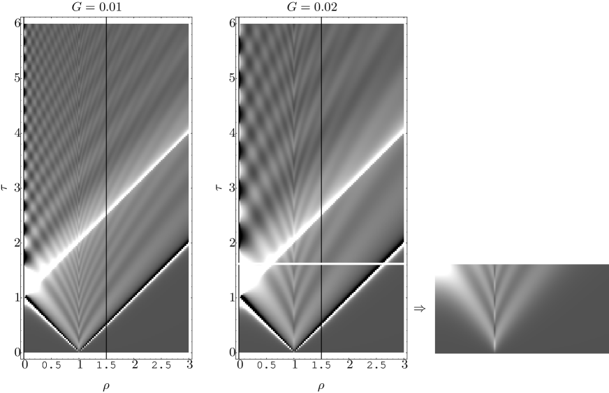
Figure 2: Density plot of the asymptotic approximation in $\lambda$ for the field commutator (over $8iG$) as a function of $(\rho,\tau)$ for $G=0.01$ and $G=0.02$. Notice the singular behavior of the approximation in the boundaries between the regions I, II, III, and on the axis. For comparison we show part of the plot for $G=0.02$ obtained with the series expansion (16). Sections of these plots for $\rho=0$ and $\rho=1.5$ with $G=0.02$ are shown in figs. 3 and 4.

Figure 3: Asymptotic approximation in $\lambda$ for the field commutator (over $8iG$) as a function of $\tau$ for $\rho=0$ and $G=0.02$. We plot, for comparison, the commutator corresponding to the free Hamiltonian discussed in Barbero G. et al. (2003). The solid line corresponds to a numerical computation of (4). As can be seen the asymptotic approximation is very good for most of the values of $\tau$.

Figure 4: Asymptotic approximation in $\lambda$ for the field commutator (over $8iG$) as a function of $\tau$ for $\rho=1.5$ and $G=0.02$. We plot, as before, the contribution corresponding to the free Hamiltonian and a numerical computation of the commutator.

Comparison with the results of numerical integration confirm the accuracy of the approximation provided by the asymptotic expressions, as long as one is far enough from the boundary between regions. This is shown in figs. 3 and 4, where we compare the asymptotic approximation with the result obtained by numerically computing the field commutator at $\rho=0$ and $\rho=1.5$.

The limit $\lambda\rightarrow 0$ is directly obtained by truncating (16) to the desired number of terms.

III Asymptotic analysis: Mathematical details

We discuss in detail here the techniques used to obtain the asymptotic expansions discussed in the previous section. Even though we will be mostly employing standard techniques it is nonetheless necessary to adapt them to the different parameters that appear in the problem, ($\rho$, $\tau$, $\lambda$). Before studying the asymptotic expansions we present some results on Mellin transforms and explain the basics of their use to obtain the asymptotic behavior of integrals.

Whenever possible it will prove useful to write the integrals under consideration as $h$-transforms, i.e. objects of the type

$$H[f;\zeta]:=\int_{0}^{\infty}h(\zeta t)f(t)dt$$

where $\zeta$ is the asymptotic parameter (that in practice approaches either 0 or $\infty$) and $f$ and $h$ are locally integrable functions in $(0,\infty)$ [functions that are integrable in every closed interval in $(0,\infty)$]. This will allow us, in many cases, to employ standard asymptotic techniques (see e.g. Bleistein and Handelsman (1986)) based on Mellin transforms that can be summarized in the following

theorem: Let $h:(0,\infty)\mapsto\mathbb{C}$ and $f:(0,\infty)\mapsto\mathbb{C}$ be locally integrable functions. Let us assume that they respectively have the following asymptotic expansions when $t\rightarrow\infty$ and $t\rightarrow 0^{+}$:

$$h(t)\sim e^{-dt^{\nu}}\sum_{m=0}^{\infty}\sum_{n=0}^{N(m)}c_{mn}t^{-r_{m}}(\log t)^{n}$$ (17)

[$\Re(d)\geq 0$, $\nu>0$, $\Re(r_{m})$ grows monotonically to $\infty$, and $N(m)>0$ is a finite integer for each value of $m$] and

$$f(t)\sim e^{-qt^{\mu}}\sum_{m=0}^{\infty}\sum_{n=0}^{\bar{N}(m)}p_{mn}t^{a_{m}}(\log t)^{n}$$ (18)

[$\Re(q)\geq 0$, $\mu>0$, $\Re(a_{m})$ grows monotonically to $\infty$ and $\bar{N}(m)>0$ is a finite integer for each value of $m$].

Let $M[h;z]$ and $M[f;z]$ be the Mellin transforms of $h$ and $f$ (in the generalized sense, see Bleistein and Handelsman (1986) for details), holomorphic in the strips $\alpha<\Re(z)<\beta$ and $\gamma<\Re(z)<\delta$ that we assume overlapping. Let us suppose also that the Parseval identity holds:

$$H[f;\zeta]=\frac{1}{2\pi i}\int_{r-i\infty}^{r+i\infty}\!\!dz\zeta^{-z}M[h;z]M[f;1-z]\equiv\frac{1}{2\pi i}\int_{r-i\infty}^{r+i\infty}\!\!dz\zeta^{-z}G(z)$$ (19)

with $r$ in the intersection of the holomorphicity strips. If $\lim_{|y|\rightarrow\infty}G(x+iy)=0$ for each $x\in[r,R]$, ($R\in\mathbb{R}$) and $\int_{-\infty}^{\infty}dy|G(R+iy)|$ is finite then

$$H[f;\zeta]\sim-\!\!\!\!\!\!\sum_{r<\Re(z)<R}{\rm res}(\zeta^{-z}M[h;z]M[f;1-z])$$

is a finite asymptotic expansion of $H[f;\zeta]$ as $\zeta\rightarrow\infty$ with respect to the asymptotic sequence $\Phi_{j,m}(\zeta)=\{\zeta^{-\alpha_{j}}(\log\zeta)^{n_{j}-m}\}$, $m=0,\,1,\ldots,n$, $j=0,\,1,\ldots$ with error $O(\zeta^{-R})$. If the previous hypotheses hold for arbitrary values of $R$ we get an asymptotic expansion with an infinite number of terms.

In the following we will only need to consider the case when $d\neq 0$ and $q=0$. The result of the previous theorem can be written as

$$H[f;\zeta]\sim\sum_{m=0}^{\infty}\zeta^{-1-a_{m}}\sum_{n=0}^{\bar{N}(m)}p_{mn}\sum_{j=0}^{n}\left(\begin{array}[]{c}n\\ j\end{array}\right)(-\log\zeta)^{j}M^{(n-j)}[h;z]\Big{|}_{z=1+a_{m}}$$ (20)

with $M^{(k)}[h;z]$ denoting the $k^{\rm{th}}$ derivative of the Mellin transform with respect to to $z$.

III.1 Asymptotic behavior in $\rho$

We write the integral that gives the field commutator in the form (5) and choose $\rho$ as the asymptotic parameter. In order to apply the previous theorem we need the asymptotic expansion of $f(t)=J_{0}(t)e^{i\tau\lambda(1-e^{-t/\lambda})}$ as $t\rightarrow 0^{+}$ and the Mellin transform of $h(t)=J_{0}(t)$. From the first we get $a_{k}=k$, ($k=0,\,1,\ldots$), $p_{00}=1,\,p_{10}=i\tau$, etc. The Mellin transform of $h$ is given by

$$M[h;z]=\frac{2^{z-1}\Gamma(z/2)}{\Gamma(1-z/2)}.$$

Since $M[h;k]=0$ for even values of $k$, we get the asymptotic expansion in odd powers of $1/\rho$ given in (6).

In order to obtain the asymptotic expansion of the commutator when $\rho\rightarrow 0^{+}$ we change variables in (5) according to $s=\rho t$,

$$\frac{1}{\rho R_{1}}\Im\bigg{\{}\int_{0}^{\infty}ds\,J_{0}(s)J_{0}\left(\frac{s}{\rho}\right)e^{i\tau\lambda(1-e^{-\frac{s}{\rho\lambda}})}\bigg{\}},$$

take $1/\rho$ as the asymptotic parameter, and switch the roles of $f$ and $h$ Bleistein and Handelsman (1986) [$f(s)=J_{0}(s)$, $h(s)=J_{0}(s)e^{i\tau\lambda(1-e^{-s/\lambda})}$]. The Mellin transform of $h$ is given now by

$$M[h;z]=\int_{0}^{\infty}dt\,t^{z-1}J_{0}(t)e^{i\tau\lambda(1-e^{-t/\lambda})},$$

which converges in the strip $0<\Re(z)<3/2$. We do not know any closed expression for this integral but it suffices to obtain the first term of the asymptotic expansion of the commutator when $\rho\rightarrow 0^{+}$. The asymptotic expansion of $f$ gives now $a_{k}=2k$, ($k=0,\,1,\ldots$), $p_{00}=1,\,p_{10}=-1/4$, etc. and using the theorem we obtain the expansion (7). Under mild restrictions Bleistein and Handelsman (1986) it can be shown that $M[h;z]$ admits an analytic continuation for $\Re(z)\rightarrow\infty$ which is meromorphic, at worst, in the complex plane, and that can be used to get further terms of the analytic expansion as $\rho\rightarrow 0^{+}$. Notice, however, that beyond the first term we cannot use the integral representation of the Mellin transform of $h$ given above because the integral becomes divergent for $z=2k$; $k\geq 1$. This prevents us from getting further terms in the asymptotic expansion as $\rho\rightarrow 0^{+}$ by using this method.

III.2 Asymptotic behavior in $\tau$

The integral in (4) is not an $h$-transform when $\tau$ is chosen as the asymptotic parameter but can be written as such by using the change of variables $u=\lambda e^{-t/\lambda}$. This gives

$$\frac{\lambda}{R_{1}}\Im\bigg{\{}e^{i\tau\lambda}\int_{0}^{\lambda}du\frac{e^{-i\tau u}}{u}J_{0}\left(\lambda\log\frac{u}{\lambda}\right)J_{0}\left(\rho\lambda\log\frac{u}{\lambda}\right)\bigg{\}}.$$ (21)

Even though this integral has now the appropriate form with $f(u)=\frac{1}{u}\chi_{[0,\lambda]}(u)J_{0}(\lambda\log\frac{u}{\lambda})J_{0}(\rho\lambda\log\frac{u}{\lambda})$ and $h(u)=e^{-iu}$, the asymptotic behavior of $f(u)$ as $u\rightarrow 0^{+}$ is not of the type considered in the theorem. This has some unpleasant consequences, the Mellin transform of $f$ cannot be analytically continued as a meromorphic function on $\mathbb{C}$, and we cannot use the expressions given in the theorem for the asymptotic behavior of $h$-transforms. This forces us to follow a more complicated approach. We will consider the cases $\rho=0$ and $\rho\neq 0$ separately.

III.2.1 $\rho=0$

We have to study the integral

$$\frac{\lambda}{R_{1}}\Im\bigg{\{}e^{i\tau\lambda}\int_{0}^{\lambda}du\frac{e^{-i\tau u}}{u}J_{0}\left(\lambda\log\frac{u}{\lambda}\right)\bigg{\}}$$ (22)

when $\tau\rightarrow\infty$. Let us set $h(u)=e^{-i\tau u}$ and $f(u)=\chi_{[0,\lambda]}(u)\frac{1}{u}J_{0}(\lambda\log\frac{u}{\lambda})$ [remember that $h$-transforms are defined as integrals over $(0,\infty)$]. The Mellin transforms of these functions are

$$M[h;z]=\tau^{-z}\Gamma(z)e^{-i\pi z/2},$$

convergent in the strip $0<\Re(z)<1$, and

$$M[f;z]=\frac{\lambda^{z-1}}{\sqrt{\lambda^{2}+(z-1)^{2}}},$$

which converges in $1<\Re(z)$. Several comments are in order. First we see that the Mellin transform of $f$ cannot be analytically continued as a meromorphic function over the complex plane because of the cuts coming from the square root. If we choose the branch given by $\log(z)=\log|z|+i\arg(z)$ with $\arg(z)\in(-\pi,\pi]$ the cuts are those parts of the imaginary axis with $|z|\geq\lambda$. Another comment is that the regions where the Mellin transforms converge do not overlap; this fact precludes us from directly employing the Mellin-Parseval formula (19). The reason can be traced back to the behavior of $h(t)$ as $t\rightarrow 0^{+}$; fortunately this problem can be fixed in a straightforward way. First we rewrite (22) as

$$\frac{\lambda}{R_{1}}\Im\bigg{\{}e^{i\tau\lambda}\int_{0}^{\lambda}du\frac{(e^{-i\tau u}-1)}{u}J_{0}\left(\lambda\log\frac{u}{\lambda}\right)\bigg{\}}+\frac{i\lambda}{R_{1}}\Im\bigg{\{}e^{i\tau\lambda}\int_{0}^{\lambda}du\frac{1}{u}J_{0}\left(\lambda\log\frac{u}{\lambda}\right)\bigg{\}}$$

$$=\frac{1}{R_{1}}\Im\bigg{\{}e^{i\tau\lambda}\Big{[}1+\lambda\int_{0}^{\lambda}du\frac{(e^{-i\tau u}-1)}{u}J_{0}\left(\lambda\log\frac{u}{\lambda}\right)\Big{]}\bigg{\}}.$$

In order to study the last integral, we choose $f(u)$ as above and $h(u)=\chi_{[0,\lambda]}(u)[e^{-i\tau u}-1]$. The Mellin transform of $h$ can be written in terms of confluent hypergeometric functions but one can work with a simpler expression by realizing that, since $f(u)$ is zero if $u>\lambda$, one can replace $h$ with a new function $\tilde{h}$ that differs from it only for $u>\lambda$:

$$\tilde{h}:\mathbb{R}^{+}\rightarrow\mathbb{R}:s\mapsto\left\{\begin{array}[]{ll}e^{-i\tau s}-1&s\in(0,\lambda)\\ e^{-i\tau s}&s\in[\lambda,\infty)\end{array}\right..$$

The result is easily seen to be independent of this extension of $h$. The integral giving the Mellin transform of $\tilde{h}$ converges in the strip $-1<\Re(z)<1$ with $M[\tilde{h};z]=\tau^{-z}\Gamma(z)e^{-i\pi z/2}-\frac{\lambda^{z}}{z}$. Since we now have overlapping convergence strips we can use the Mellin-Parseval formula and obtain a Mellin-Barnes representation of our integral as

$$\frac{1}{R_{1}}\Im\bigg{\{}e^{i\tau\lambda}\left[1+\frac{\lambda}{2\pi i}\int_{c-i\infty}^{c+i\infty}\!\!dz\frac{\tau^{-z}\lambda^{-z}\Gamma(z)e^{-i\pi z/2}-\frac{1}{z}}{\sqrt{\lambda^{2}+z^{2}}}\right]\bigg{\}}$$

$$=\frac{1}{R_{1}}\Im\bigg{\{}e^{i\tau\lambda}\left[1+\frac{\lambda}{2\pi i}\int_{c-i\infty}^{c+i\infty}\!\!dz\frac{\tau^{-z}\lambda^{-z}\Gamma(z)e^{-i\pi z/2}}{\sqrt{\lambda^{2}+z^{2}}}\right]\bigg{\}}$$ (24)

with $\Re(c)\in(-1,0)$. We have employed the fact that

$$\int_{c-i\infty}^{c+i\infty}\!\!dz\frac{dz}{z\sqrt{\lambda^{2}+z^{2}}}=0.$$

The analytic continuation of the integrand in the r.h.s. of (24) is immediate. It has algebraic singularities at $z=\pm i\lambda$ (see fig. 5) with cuts in those points of the imaginary axis where $|z|>\lambda$, and simple poles on $-z\in\mathbb{N}\cup\{0\}$.

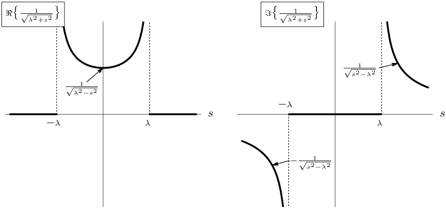
Figure 5: Real and imaginary parts of $\frac{1}{\sqrt{\lambda^{2}+z^{2}}}$ on the curve $z=-0^{+}+is$ (corresponding to $\rho=0$). In the vicinity of the singularities at $is=\pm i\lambda$ the real and imaginary parts of this function behave as $\frac{1}{\sqrt{2\lambda(\lambda\mp s)}}\quad(|s|<\lambda)$ and $\frac{\pm 1}{\sqrt{2\lambda(\pm s-\lambda)}}\quad(|s|>\lambda)$.

In order to study the limit $\tau\rightarrow 0^{+}$ we can displace the integration contour in (24) leftwards parallel to the imaginary axis. A simple analysis using the asymptotics of $\Gamma(z)$ for large values of $\Im(z)$ shows that the series given by the residues of the integrand at the poles $-z\in\mathbb{N}$, namely

$$\frac{\lambda}{R_{1}}\Im\bigg{\{}e^{i\tau\lambda}\sum_{k=0}^{\infty}\frac{(-i\lambda\tau)^{k}}{k!\sqrt{\lambda^{2}+k^{2}}}\bigg{\}},$$

converges to the value of the integral. This is precisely what one would get by expanding the exponential in (22), exchanging sum and integration, and computing the integrals that appear. This was the procedure used in Barbero G. et al. (2003).

It is not possible to directly get the asymptotic behavior in the $\tau\rightarrow\infty$ limit by displacing the integration contour rightwards because of the presence of the cut and, even worse, the absence of poles with $\Re(z)\geq 0$. One could consider choosing a value for $c$ and write (24) as a real integral in the variable $y\in\mathbb{R}$ after the change $z=c+iy$. In fact, by doing that one obtains the sum of two $h$-transforms with asymptotic parameter $\log\tau$ that can be studied with the standard formulas. Unfortunately, proceeding in this way one gets a trivial zero asymptotic expansion. The reason, as we will find out later on, is that $\log\tau$ is almost, but not quite, the right asymptotic parameter.

The solution to our problem is displacing the integration contour all the way to the cut (choosing $c\rightarrow 0^{-}$) as shown in fig. 6.

Figure 6: Cuts and singularities of the integrand and integration contours in the complex plane for the Mellin-Barnes representation used in the asymptotic analysis for $\tau\rightarrow\infty$ in the cases $\rho=0$ and $\rho\neq 0$.

The contribution of the arcs $\Gamma_{2}$ and $\Gamma_{4}$ to the integral in the r.h.s. of (24) goes to zero as $-c=\epsilon\rightarrow 0^{+}$. The remaining three contributions to the integral (without prefactors) are

$$\Gamma_{1}\quad\quad-\int_{\lambda}^{\infty}dy\frac{e^{-iy\log(\lambda\tau)}e^{\pi y/2}\Gamma(iy)}{\sqrt{y^{2}-\lambda^{2}}},$$

$$\Gamma_{3}\quad\quad-\frac{\pi i}{\lambda}+i{\rm P.V.}\int_{-\lambda}^{\lambda}dy\frac{e^{-iy\log(\lambda\tau)}e^{\pi y/2}\Gamma(iy)}{\sqrt{\lambda^{2}-y^{2}}},$$

$$\Gamma_{5}\quad\quad\int_{-\infty}^{-\lambda}dy\frac{e^{-iy\log(\lambda\tau)}e^{\pi y/2}\Gamma(iy)}{\sqrt{y^{2}-\lambda^{2}}}.$$

The asymptotic expansions of these integrals can be obtained by a variety of methods, for example by steepest descents. Nonetheless, it is now possible to employ formula (20) and obtain, in principle, the asymptotics to any order.

The integral over $\Gamma_{1}$ can be written as the following standard $h$-transform by the change of variables $y=\lambda(1+s)$ with $s\in[0,\infty)$:

$$-e^{-i\lambda\log(\lambda\tau)}e^{\pi\lambda/2}\int_{0}^{\infty}ds\,e^{-i\lambda s\log\tau}\frac{e^{-i\lambda s\log\lambda}e^{\pi\lambda s/2}\Gamma[i\lambda(1+s)]}{\sqrt{s(s+2)}}.$$

Taking $h(z)=e^{-i\lambda z}$, $f(z)=\frac{e^{-i\lambda z\log\lambda}e^{\pi\lambda z/2}\Gamma[i\lambda(1+z)]}{\sqrt{z(z+2)}}$, and the asymptotic parameter $\log\tau$ we can use formulas (19) and (20). Since the asymptotic behavior of $f$ when $z\rightarrow 0^{+}$ is

$$f(z)\sim\frac{\Gamma(i\lambda)}{\sqrt{2z}}+O(z^{1/2})$$

and $M[h;z]=\lambda^{-z}e^{-\frac{\pi iz}{2}}\Gamma(z)$, we get for the integral over $\Gamma_{1}$ an asymptotic expansion in powers of $1/\sqrt{\log\tau}$ with a $\tau$ oscillating factor $e^{-i\lambda\log(\lambda\tau)}$, namely

$$-e^{-i\lambda\log(\lambda\tau)+\frac{\pi\lambda}{2}-\frac{\pi i}{4}}\Gamma(i\lambda)\bigg{\{}\sqrt{\frac{\pi}{2\lambda\log\tau}}+O\bigg{[}\frac{1}{(\log\tau)^{3/2}}\bigg{]}\bigg{\}}.$$

A similar argument can be used to calculate the asymptotic expansion of the integral over $\Gamma_{5}$,

$$e^{i\lambda\log(\lambda\tau)-\frac{\pi\lambda}{2}+\frac{\pi i}{4}}\Gamma(-i\lambda)\bigg{\{}\sqrt{\frac{\pi}{2\lambda\log\tau}}+O\bigg{[}\frac{1}{(\log\tau)^{3/2}}\bigg{]}\bigg{\}}.$$

Finally, to get the asymptotics of the integral over $\Gamma_{3}$ we express it in the form

$$-\frac{\pi i}{\lambda}+i\int_{0}^{\lambda}dy\cos[y\log\tau]\frac{e^{-iy\log\lambda}e^{\pi y/2}\Gamma(iy)+e^{iy\log\lambda}e^{-\pi y/2}\Gamma(-iy)}{\sqrt{\lambda^{2}-y^{2}}}\hskip 17.07182pt$$

$$-i\int_{0}^{\lambda}dy\sin[y\log\tau]\frac{e^{iy\log\lambda}e^{-\pi y/2}\Gamma(-iy)-e^{-iy\log\lambda}e^{\pi y/2}\Gamma(iy)}{\sqrt{\lambda^{2}-y^{2}}}\quad\,\,.$$

By introducing neutralizers as in Bleistein and Handelsman (1986) it is possible to show that the critical points for the previous two integrals are 0 and $\lambda$. The contributions to the asymptotic expansion from both points can be obtained in a straightforward way using formula (20). The contribution from zero is $-\frac{\pi i}{\lambda}$ whereas the one from $\lambda$ coincides precisely with the sum of the contributions obtained before for $\Gamma_{1}$ and $\Gamma_{5}$. Summing all the terms and substituting the result in (24) we finally get the behavior in $\tau$ presented in Section II.

It is worth remarking that the asymptotic expansions discussed can be written as an oscillating factor that depends on $\log\tau$ multiplying an expansion in terms of inverse powers of $\sqrt{\log\tau}$. Moreover, note that the frequency of these oscillations is exactly that of the oscillating factor that we have already obtained.

III.2.2 $\rho\neq 0$

Consider now the integral (21). We set $h(u)=e^{-i\tau u}$ and $f(u)=\chi_{[0,\lambda]}(u)\frac{1}{u}J_{0}(\lambda\log\frac{u}{\lambda})J_{0}(\rho\lambda\log\frac{u}{\lambda})$. The Mellin transform of $f$ is

$$M[f;z]=\frac{\lambda^{z-2}}{\pi\sqrt{\rho}}Q_{-\frac{1}{2}}\left[\frac{\lambda^{2}(1+\rho^{2})+(z-1)^{2}}{2\rho\lambda^{2}}\right].$$

Proceeding as in the $\rho=0$ case we get the following Mellin-Barnes representation:

$$\frac{1}{\pi R_{1}\sqrt{\rho}}\Im\bigg{\{}e^{i\tau\lambda}\bigg{[}Q_{-\frac{1}{2}}\left(\frac{1+\rho^{2}}{2\rho}\right)+\frac{1}{2\pi i}\int_{c-i\infty}^{c+i\infty}\!\!\!\!dz\left(\tau^{-z}\lambda^{-z}\Gamma(z)e^{-i\pi z/2}-\frac{1}{z}\right)Q_{-\frac{1}{2}}\left(\frac{\lambda^{2}(1+\rho^{2})+z^{2}}{2\rho\lambda^{2}}\right)\bigg{]}\bigg{\}}$$

$$=\frac{1}{\pi R_{1}\sqrt{\rho}}\Im\bigg{\{}e^{i\tau\lambda}\bigg{[}Q_{-\frac{1}{2}}\left(\frac{1+\rho^{2}}{2\rho}\right)+\frac{1}{2\pi i}\int_{c-i\infty}^{c+i\infty}\!\!\!\!dz\,\,\tau^{-z}\lambda^{-z}e^{-i\pi z/2}\Gamma(z)Q_{-\frac{1}{2}}\left(\frac{\lambda^{2}(1+\rho^{2})+z^{2}}{2\rho\lambda^{2}}\right)\bigg{]}\bigg{\}}.$$ (25)

The main difference with the previous case is the appearance of the associated Legendre function $Q_{-\frac{1}{2}}$. This function has cuts on the imaginary axis for $|\Im(z)|\geq\lambda|\rho-1|$. On the left of the cut the real and imaginary parts behave as shown in fig. 7. They become singular in the neighborhood of the four points $z=\pm i\lambda|\rho-1|$ and $z=\pm i\lambda(\rho+1)$. The real functions that describe each of the continuous pieces are shown in the plots. Some of them are given by $Q_{-\frac{1}{2}}(x)$ evaluated on $x>1$. Quite surprisingly, the others can be written in terms of the associated Legendre function $P_{-\frac{1}{2}}$ [$P_{-\frac{1}{2}}(x)=F\left(\frac{1}{2},\frac{1}{2};1;\frac{1-x}{2}\right)$] with argument $x>-1$. The fundamental consequence of this is a change in the singularity structure of the integrand of (25).

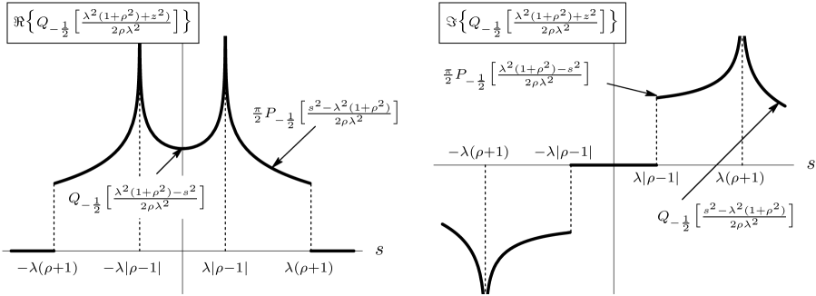
Figure 7: Real and imaginary parts of $Q_{-\frac{1}{2}}\big{[}\frac{\lambda^{2}(1+\rho^{2})+z^{2}}{2\rho\lambda^{2}}\big{]}$ on the curve $z=-0^{+}+is$ for $\rho\neq 0$.

The limit $\tau\rightarrow 0^{+}$ can be obtained as we did for $\rho=0$. The result is given by (16).

By displacing the integration contour rightwards to the cut as in the $\rho=0$ case (see fig. 6) we can split the last integral in (25) into seven different contributions corresponding to the integration curves $\gamma_{1},\ldots,\gamma_{7}$. It is straightforward to show that the contributions from $\gamma_{3}$ and $\gamma_{5}$ go to zero as the contour gets closer to the imaginary axis. We are then left with

$$\gamma_{1}\quad\quad\hskip 2.84526pt-\int_{\lambda(\rho+1)}^{\infty}dy\hskip 5.69054pte^{-iy\log(\lambda\tau)}e^{\pi y/2}\Gamma(iy)Q_{-\frac{1}{2}}\left(\frac{y^{2}-\lambda^{2}(1+\rho^{2})}{2\rho\lambda^{2}}\right),$$

$$\gamma_{2}\quad\quad\frac{\pi}{2}i\int_{\lambda|\rho-1|}^{\lambda(\rho+1)}dy\hskip 5.69054pte^{-iy\log(\lambda\tau)}e^{\pi y/2}\Gamma(iy)\bigg{[}P_{-\frac{1}{2}}\left(\frac{y^{2}-\lambda^{2}(1+\rho^{2})}{2\rho\lambda^{2}}\right)+iP_{-\frac{1}{2}}\left(\frac{\lambda^{2}(1+\rho^{2})-y^{2}}{2\rho\lambda^{2}}\right)\bigg{]},$$

$$\gamma_{4}\quad\quad-i\pi Q_{-\frac{1}{2}}\left(\frac{1+\rho^{2}}{2\rho}\right)+iP.V.\int_{-\lambda|\rho-1|}^{\lambda|\rho-1|}dy\hskip 5.69054pte^{-iy\log(\lambda\tau)}e^{\pi y/2}\Gamma(iy)Q_{-\frac{1}{2}}\left(\frac{\lambda^{2}(1+\rho^{2})-y^{2}}{2\rho\lambda^{2}}\right),$$

$$\gamma_{6}\quad\quad\frac{\pi}{2}i\int_{-\lambda(\rho+1)}^{-\lambda|\rho-1|}dy\hskip 5.69054pte^{-iy\log(\lambda\tau)}e^{\pi y/2}\Gamma(iy)\bigg{[}P_{-\frac{1}{2}}\left(\frac{y^{2}-\lambda^{2}(1+\rho^{2})}{2\rho\lambda^{2}}\right)-iP_{-\frac{1}{2}}\left(\frac{\lambda^{2}(1+\rho^{2})-y^{2}}{2\rho\lambda^{2}}\right)\bigg{]},$$

$$\gamma_{7}\quad\quad\quad\int_{-\infty}^{-\lambda(\rho+1)}dy\hskip 5.69054pte^{-iy\log(\lambda\tau)}e^{\pi y/2}\Gamma(iy)Q_{-\frac{1}{2}}\left(\frac{y^{2}-\lambda^{2}(1+\rho^{2})}{2\rho\lambda^{2}}\right).$$

All these integrals can be written as Fourier transforms whose only critical points are the integration limits. These can be isolated by using the appropriate neutralizers Bleistein and Handelsman (1986) and the integrals so obtained can be written as $h$-transforms by straightforward changes of variables. An interesting feature of some of the integrals that arise is the fact that the asymptotic expansion of the corresponding $f$ functions involve logarithms precisely in the form assumed in (18). This means that in addition to the $p_{m0}$ coefficients that appeared in the $\rho=0$ case we will have also contributions coming from the $p_{mn}$’s with $n\neq 0$.

In order to get the asymptotic behavior of the different $f$ functions close to their singularities it is useful to remember the asymptotic expansions of $P_{-\frac{1}{2}}(x)$ and $Q_{-\frac{1}{2}}(x)$ at $x=-1^{+}$ and $x=1^{+}$, respectively:

$$P_{-\frac{1}{2}}(x)\sim\frac{5}{\pi}\log 2-\frac{1}{\pi}\log(x+1)+\cdots$$

$$Q_{-\frac{1}{2}}(x)\sim\frac{5}{2}\log 2-\frac{1}{2}\log(x-1)+\cdots$$

With the previous guidelines, and following the same steps as in the $\rho=0$ case, it is easy (albeit lengthy) to deduce (9). It is possible to arrive at the same result by different methods that are somewhat simpler (i.e. steepest descents) but they only allow to compute the first contribution to the asymptotic behavior of the field commutator. The advantage of the method employed here is that one can calculate as many terms as desired for the asymptotic expansion just by taking more terms in the asymptotic series of the function $f$.

III.3 Asymptotic behavior in $\lambda$

We will consider now integrals of the form

$$\int_{B}^{A}dq\oint_{\gamma_{1}}dt_{1}\oint_{\gamma_{2}}dt_{2}f_{(0)}(q;t_{1},t_{2})e^{\lambda\Phi(q;t_{1},t_{2})}$$ (26)

($0\leq B<A$) where $q$ is a real variable, $t_{1}$ and $t_{2}$ are complex variables and $\gamma_{1,2}$ are closed paths (possibly different) in the complex plane. The functions $f_{(0)}$ and $\Phi$ are supposed to be holomorphic in the two complex arguments and $C^{n}$ in $q$ (with $n$ possibly infinite) in an open neighborhood of the integration region. In the following we will use the notation $\partial_{i}\equiv\partial_{t_{i}},\,\,i=1,\,2$, $\nabla\equiv(\partial_{q},\partial_{1},\partial_{2})$, and $||\nabla\Phi||^{2}\equiv\eta_{q}(\partial_{q}\Phi)^{2}+\eta_{t_{1}}(\partial_{1}\Phi)^{2}+\eta_{t_{2}}(\partial_{2}\Phi)^{2}$, where $\eta_{q}$, $\eta_{t_{1}}$, and $\eta_{t_{2}}$ are some functions of $q$, $t_{1}$, and $t_{2}$ that will be chosen later in the discussion. This freedom will prove to be useful when we parametrize the curves $\gamma_{1,2}$ because it will allow us to have denominators in the integrand that are real positive functions, facilitating the analysis of the $A\rightarrow\infty$ limit. If $\|\nabla\Phi\|^{2}$ differs from zero for all $q\in[B,A]$, $t_{1}\in\gamma_{1}$, and $t_{2}\in\gamma_{2}$, it is possible to devise an “integration by parts” procedure for this type of integrals by writing them as

$$\frac{1}{\lambda}\int_{B}^{A}dq\oint_{\gamma_{1}}dt_{1}\oint_{\gamma_{2}}dt_{2}\bigg{[}\frac{f_{(0)}\eta_{q}\partial_{q}\Phi\partial_{q}e^{\lambda\Phi}}{\|\nabla\Phi\|^{2}}+\frac{f_{(0)}\eta_{t_{1}}\partial_{1}\Phi\partial_{1}e^{\lambda\Phi}}{\|\nabla\Phi\|^{2}}+\frac{f_{(0)}\eta_{t_{2}}\partial_{2}\Phi\partial_{2}e^{\lambda\Phi}}{\|\nabla\Phi\|^{2}}\bigg{]}.$$

The contribution of the first term can be written, after integrating by parts in $q$, as

$$\frac{1}{\lambda}\oint_{\gamma_{1}}dt_{1}\oint_{\gamma_{2}}dt_{2}\frac{f_{(0)}\eta_{q}\partial_{q}\Phi e^{\lambda\Phi}}{\|\nabla\Phi\|^{2}}\Bigg{|}_{B}^{A}-\frac{1}{\lambda}\oint_{\gamma_{1}}dt_{1}\oint_{\gamma_{2}}dt_{2}\int_{B}^{A}dqe^{\lambda\Phi}\partial_{q}\frac{f_{(0)}\eta_{q}\partial_{q}\Phi}{\|\nabla\Phi\|^{2}}$$

(notice that the integration region is compact and the function integrable so that we can apply Fubini’s theorem and freely exchange orders of integration). Integration by parts in $t_{1}$ gives

$$\frac{1}{\lambda}\int_{B}^{A}dq\oint_{\gamma_{2}}dt_{2}\oint_{\gamma_{1}}dt_{1}\partial_{1}\frac{f_{(0)}\eta_{t_{1}}\partial_{1}\Phi e^{\lambda\Phi}}{\|\nabla\Phi\|^{2}}-\frac{1}{\lambda}\int_{B}^{A}dq\oint_{\gamma_{2}}dt_{2}\oint_{\gamma_{1}}dt_{1}e^{\lambda\Phi}\partial_{1}\frac{f_{(0)}\eta_{t_{1}}\partial_{1}\Phi}{\|\nabla\Phi\|^{2}}.$$

If $(f_{(0)}\eta_{t_{1}}\partial_{1}\Phi e^{\lambda\Phi})\|\nabla\Phi\|^{-2}$ is a holomorphic function of $t_{1}$ in an open set containing the closed curve $\gamma_{1}$ (for all $q\in[B,A]$ and $t_{2}\in\gamma_{2}$) the first integral is zero and we are left only with the second term. The same argument applies to the integration in $t_{2}$. We finally get that (26) can be written as

$$\frac{1}{\lambda}\oint_{\gamma_{1}}dt_{1}\oint_{\gamma_{2}}dt_{2}\frac{f_{(0)}\eta_{q}\partial_{q}\Phi e^{\lambda\Phi}}{\|\nabla\Phi\|^{2}}\Bigg{|}_{B}^{A}-\frac{1}{\lambda}\int_{B}^{A}dq\oint_{\gamma_{1}}dt_{1}\oint_{\gamma_{2}}dt_{2}f_{(1)}(q;t_{1},t_{2})e^{\lambda\Phi(q;t_{1},t_{2})},$$ (27)

here we have introduced the notation

$$f_{(k+1)}\equiv\partial_{q}\frac{f_{(k)}\eta_{q}\partial_{q}\Phi}{\|\nabla\Phi\|^{2}}+\partial_{1}\frac{f_{(k)}\eta_{t_{1}}\partial_{1}\Phi}{\|\nabla\Phi\|^{2}}+\partial_{2}\frac{f_{(k)}\eta_{t_{2}}\partial_{2}\Phi}{\|\nabla\Phi\|^{2}}\quad k=0,\,1,\ldots.$$

The second integral in (27) has the same structure as the original integral, so the same procedure can be applied as long as the appropriate regularity conditions are satisfied for expressions involving the successive $f_{(k)}$, $k=1,\ldots$ The strategy to obtain asymptotic expansions for the original integral consists in getting expansions for the lower dimensional boundary integrals that arise in this way, provided that the remaining non-boundary integral behaves nicely in the $\lambda\rightarrow\infty$ limit. Particularizing this argument to the case of a single complex variable $t$ is straightforward.

In our case [see equation (10)] we actually want to obtain an asymptotic expansion of an improper integral. So we will also have to study the asymptotics of the limit $A\rightarrow\infty$,

$$-\frac{1}{\lambda}\oint_{\gamma_{1}}dt_{1}\oint_{\gamma_{2}}dt_{2}\frac{f_{(0)}\eta_{q}\partial_{q}\Phi e^{\lambda\Phi}}{\|\nabla\Phi\|^{2}}\Bigg{|}_{B}$$ (28)

$$+\lim_{A\rightarrow\infty}\bigg{\{}\frac{1}{\lambda}\oint_{\gamma_{1}}dt_{1}\oint_{\gamma_{2}}dt_{2}\frac{f_{(0)}\eta_{q}\partial_{q}\Phi e^{\lambda\Phi}}{\|\nabla\Phi\|^{2}}\Bigg{|}_{A}-\frac{1}{\lambda}\int_{B}^{A}dq\oint_{\gamma_{1}}dt_{1}\oint_{\gamma_{2}}dt_{2}f_{(1)}(q;t_{1},t_{2})e^{\lambda\Phi(q;t_{1},t_{2})}\bigg{\}}.$$

In order to derive useful asymptotic expansions from the previous formulas it is desirable that $e^{\lambda\Phi(q;t_{1},t_{2})}$ be bounded by a $\lambda$-independent function. This happens for example if $\Re[\Phi(q;t_{1},t_{2})]\leq 0$ in the integration region $[B,A]\times\gamma_{1}\times\gamma_{2}$. In fact, we will take advantage of the freedom in the choice of the integration contours $\gamma_{1,2}$ to impose this condition.

If there are points in the integration region (referred to in the following as singular points) where $\|\nabla\Phi\|^{2}=0$ the argument presented above to derive (27) is no longer true. In such a situation the way to proceed Bleistein and Handelsman (1986); Van der Corput (1948) is to isolate them by introducing neutralizers. This allows us to divide the integration region into several pieces and study the resulting integrals by choosing the most suitable techniques. This is facilitated by the fact that neutralizers force most of the boundary integrals to be zero. In the process of obtaining asymptotic expansions from (28) it may be useful to further divide the integration region of the last integral in several pieces, by introducing additional neutralizers, in order to localize the singular points in a region that does not contain the boundary $q=A$; this simplifies the analysis of the $A\rightarrow\infty$ limit.

The freedom to choose the integration contours in (26) may be useful for other purposes. One can, for example, avoid singularities of the boundary integrals over $\{B\}\times\gamma_{1}\times\gamma_{2}$ and $\{A\}\times\gamma_{1}\times\gamma_{2}$; it may be possible to write the integrals involving the singular points as (multidimensional) Laplace or Fourier transforms for which the analysis of singular points can be carried out by standard procedures (see Bleistein and Handelsman (1986)) or to improve the behavior for large values of $q$ if one intends to study the asymptotics of the improper integral when $A\rightarrow\infty$. Finally in some cases this freedom may allow us to simplify the analysis of the contribution of some of the singular points.

As in the study of the $\tau$ asymptotics, we will consider the cases $\rho=0$ and $\rho\neq 0$ separately.

III.3.1 $\rho=0$

We study the integral (10) for $\rho=0$:

$$-\frac{1}{R_{1}}\lim_{A\rightarrow\infty}\Im\bigg{\{}\frac{i\lambda e^{i\tau\lambda}}{2\pi}\int_{0}^{A}dq\oint_{\gamma}dt\frac{1}{t}e^{\lambda\big{[}\frac{\scriptstyle q}{\scriptstyle 2}(t-\frac{\scriptstyle 1}{\scriptstyle t})-i\tau e^{-q}\big{]}}\bigg{\}}.$$ (29)

Let us discuss first the possible choices of integration contour $\gamma$. As commented above it is convenient to impose that the real part of the exponent in the integrand be less or equal to zero, i.e. $\Re(t-1/t)\leq 0$. It is straightforward to show that this happens when $u(u^{2}+v^{2}-1)\geq 0$ ($t=u+iv$). This complex region (see fig. 8) is given by the points inside the unit circle centered at the origin with positive real part, those outside this circle with negative real part, and the boundary of these two regions (i.e. the imaginary axis and the unit circumference centered at the origin). The integration contour can be any closed, positively oriented, simple curve contained in this region that surrounds the origin. Notice that all these contours contain the points $t=\pm i$.

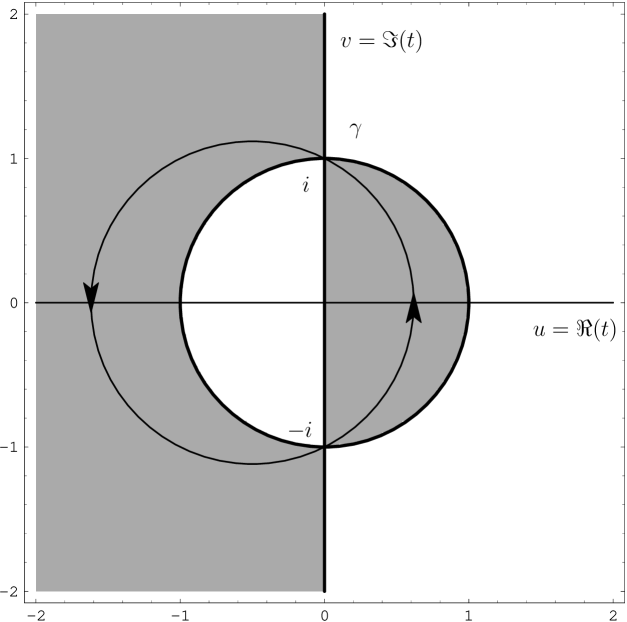
Figure 8: The region $\Re(t-1/t)\leq 0$ consists of the shadowed area and its boundary. A possible choice of the integration contour $\gamma$ is also shown.

If we choose $\eta_{q}=-1$ and $\eta_{t}=t^{2}$ we have

$$\|\nabla\Phi\|^{2}=\frac{1}{4}\left[q^{2}\,{\left(t+\frac{1}{t}\right)}^{2}-{\left(t-\frac{1}{t}+2i\tau e^{-q}\right)}^{2}\right].$$

At the left boundary ($q=0$) this is zero when $t=-i\tau\pm\sqrt{1-\tau^{2}}$. Depending on the value of $\tau$ these points may be on the unit circumference; it is, hence, convenient to choose integration contours in the allowed part of $\mathbb{C}$ that avoid them (see fig. 8). This will always be possible except for $\tau=1$. When $q\neq 0$ the condition $\|\nabla\Phi\|^{2}=0$ gives, generically, four possible solutions (depending on $q$ and $\tau$) that may or may not be in the integration region. If $\tau>1$, there is one of these, ($t=-i$, $q=\log\tau$) that will be in the integration region for every possible choice of the integration contour $\gamma$. The remaining ones will or will not belong to the integration region depending on $\gamma$. In principle one would proceed by picking a certain contour, determine the values of $q$ corresponding to these points, introduce suitable neutralizers, and study the neutralized integrals one at a time. There is, however, a simple argument that shows that it is not necessary to discuss them in detail (we assume $q\neq 0$ in the following discussion unless otherwise specified).

The idea is to write the integral in (29) as the sum of three integrals $I_{j}$, $j=1,\,2,\,3$ and choose different contours for each of them. These integrals are

$$I_{j}\equiv-\frac{1}{R_{1}}\Im\Big{\{}\frac{i\lambda e^{i\tau\lambda}}{2\pi}\int_{0}^{A}dq\oint_{\gamma}dt\,\nu_{j}(q)\frac{1}{t}e^{\lambda\big{[}\frac{\scriptstyle q}{\scriptstyle 2}(t-\frac{\scriptstyle 1}{\scriptstyle t})-i\tau e^{-q}\big{]}}\Big{\}}$$

where we have introduced three neutralizer functions $\nu_{j}(q)$, $j=1,\,2,\,3$ satisfying $\nu_{1}+\nu_{2}+\nu_{3}=1$ in $[0,A]$ and

$$\nu_{1}(q)=1\quad\textrm{if}\quad q\in[0,\alpha_{1}],$$

$$\nu_{1}(q)=0\quad\textrm{if}\quad q\in[\alpha_{2},A],$$

$$\nu_{2}(q)=0\quad\textrm{if}\quad q\in[0,\alpha_{1}]\cup[\beta_{2},A],$$

$$\nu_{2}(q)=1\quad\textrm{if}\quad q\in[\alpha_{2},\beta_{1}],$$

$$\nu_{3}(q)=0\quad\textrm{if}\quad q\in[0,\beta_{1}],$$

$$\nu_{3}(q)=1\quad\textrm{if}\quad q\in[\beta_{2},A],$$

with $0<\alpha_{1}<\alpha_{2}<\beta_{1}<\beta_{2}<A$ (the specific choices for these parameters will be explained later). By doing this the effective integration regions in $q$ are $[0,\alpha_{2}]$, $[\alpha_{1},\beta_{2}]$ and $[\beta_{1},A]$ respectively; notice that the boundary $q=0$ appears only in the first.

Let us consider first $I_{1}$. In this case it is convenient to choose an integration contour $\gamma$ that avoids the unit circumference (except at $t=\pm i$) because, if $\tau<1$, the integration by parts procedure introduced above could, otherwise, give a boundary contribution at $q=0$ involving a singular function. We pick the contour depicted in fig. 8. In order to use integration by parts it is also necessary to show that it is possible to find $\alpha_{2}$ such that $\|\nabla\Phi\|^{2}\neq 0$ in the integration region. The solutions to $\|\nabla\Phi\|^{2}=0$ are those satisfying the following quadratic equations

$$(1+q)t^{2}+2i\tau e^{-q}t-1+q=0,$$

$$(1-q)t^{2}+2i\tau e^{-q}t-1-q=0.$$

It can easily be shown (by using the implicit function theorem or the explicit solution of these equations in $t$) that the solutions are continuous at $q=0$ (if $\tau\neq 1$), i.e. the solutions for small enough $q$ are close to $t=-i\tau\pm\sqrt{1-\tau^{2}}$. If $\tau\neq 1$ it is then possible to choose $\alpha_{2}$ and $\gamma$ in such a way that $\|\nabla\Phi\|^{2}\neq 0$ in the integration region $\gamma\times[0,\alpha_{2}]$.

We can use formula (28) to get an asymptotic expansion for $I_{1}$. We first note that the term corresponding to the second integral in (27) is $O(1/\lambda)$ because our choice of contour allows us to bound the absolute value of the integrand by a regular function independent of $\lambda$. The integral $I_{1}$ is then given at leading order by the contribution of the boundary terms which can be written as

$$I_{1}=\frac{1}{\pi R_{1}}\Im\bigg{\{}i\oint_{\gamma}\frac{dt}{t^{2}+2i\tau t-1}\bigg{\}}$$

[the function $\nu_{1}(q)$ kills the contribution coming from the $q=\alpha_{2}$ boundary]. If $\tau<1$ the poles of the integrand $t=-i\tau\pm\sqrt{1-\tau^{2}}$ are on the unit circumference but only that with the negative real part is inside $\gamma$. The value of the residue of the integrand at this point is $-\frac{1}{2\sqrt{1-\tau^{2}}}$ and hence

$$I_{1}=\frac{1}{R_{1}}\Im\bigg{\{}\frac{1}{\sqrt{1-\tau^{2}}}\bigg{\}}=0.$$

If $\tau>1$ the poles of the integrand are on the imaginary axis $t=-i\tau\pm i\sqrt{\tau^{2}-1}$; now only that with the positive sign in the square root is inside $\gamma$. The residue is $\frac{1}{2i\sqrt{\tau^{2}-1}}$ and hence

$$I_{1}=\frac{1}{R_{1}}\Im\bigg{\{}\frac{i}{\sqrt{\tau^{2}-1}}\bigg{\}}=\frac{1}{R_{1}\sqrt{\tau^{2}-1}}.$$ (30)

Consider next $I_{2}$. In this case it is convenient to choose the unit circumference for $\gamma$ because, parameterizing it by an angle ($t(\theta)=e^{i\theta}$, $\theta\in(-\pi,\pi]$), the exponent $\lambda\Phi(q;t)$ becomes a purely imaginary function of the two real variables $q$ and $\theta$,

$$i\lambda\phi(q;\theta)\equiv\lambda\Phi[q;t(\theta)]=i\lambda(q\sin\theta-\tau e^{-q}),$$

and the integral becomes a Fourier transform on a rectangular region determined by the support of the neutralizer. As is well known the critical points for Fourier transforms are given by the boundaries of the integration region and those interior points where the gradient of the real function $\phi$ is zero. In our case the $q=\alpha_{1}$ and $q=\beta_{2}$ boundaries give no contribution for this integral owing to the presence of the neutralizer. Let us then find the interior critical points. Since $\|\nabla\Phi\|^{2}[q;t(\theta)]$ is a sum of squares of real numbers these points are precisely those where our procedure of integration by parts fails. We have to solve the following equations

$$q\cos\theta=0,$$

$$\sin\theta+\tau e^{-q}=0.$$

The solution is $q=0$, $\theta=-\arcsin\tau$ if $\tau<1$ (these are outside the effective integration region for $I_{2}$) and $q=\log\tau$, $\theta=-\frac{\pi}{2}$ if $\tau>1$. The choices of $\alpha_{1,2}$ can be made in such a way that the critical point with $q>0$ (present only when $\tau>1$) always corresponds to $I_{2}$ (we also choose $\beta_{1}$ such that $\log\tau<\beta_{1}$ to avoid having critical points in $I_{3}$). The asymptotic expansion of $I_{2}$ can be now obtained by using the standard formulas Bleistein and Handelsman (1986) for the contribution of critical points. In our case this is simply

$$\frac{1}{R_{1}}\Im\bigg{\{}\frac{e^{i\lambda(\tau-\log\tau-1)}}{\sqrt{\log\tau}}\bigg{\}}+O\bigg{[}\frac{1}{\lambda}\bigg{]}\hskip 28.45274pt$$ (31)

for $\tau>1$ and 0 if $\tau<1$. We do not need to discuss the limit $A\rightarrow\infty$ of $I_{1}$ and $I_{2}$ because the integrand has compact support independent of $A$; we have only assumed that $\log\tau<A$. However this is no longer true for $I_{3}$.

Let us analyze, finally, $\lim_{A\rightarrow\infty}I_{3}$. We choose again the unit circumference for $\gamma$ (with the same parametrization) and write

$$\lim_{A\rightarrow\infty}I_{3}=\Im\bigg{\{}\frac{\lambda e^{i\tau\lambda}}{2\pi R_{1}}\lim_{A\rightarrow\infty}\int_{\beta_{1}}^{A}dq\int_{-\pi}^{\pi}d\theta\,\nu_{3}(q)e^{i\lambda\phi(q;\theta)}\bigg{\}}.$$

Using formula (28) with $\eta_{q}=-1$, $\eta_{t}=t^{2}$, and taking into account that $\nu_{3}(\beta_{1})=0$, this expression becomes

$$\Im\bigg{\{}\frac{\lambda e^{i\tau\lambda}}{2\pi R_{1}}\lim_{A\rightarrow\infty}\bigg{[}\frac{-i}{\lambda}\int_{-\pi}^{\pi}d\theta\frac{(\tau e^{-A}+\sin\theta)e^{i\lambda\phi(A;\theta)}}{A^{2}\cos^{2}\theta+(\tau e^{-A}+\sin\theta)^{2}}+\frac{i}{\lambda}\int_{\beta_{1}}^{A}dq\int_{-\pi}^{\pi}d\theta\,\nu_{3}(q)e^{i\lambda\phi(q;\theta)}g_{1}(q;\theta)\bigg{]}\bigg{\}}.$$ (32)

Here

$$g_{1}(q;\theta)\equiv ie^{i\theta}f_{(1)}[q;t(\theta)]=\frac{(\tau e^{-q}+\sin\theta)^{2}(\tau e^{-q}-q\sin\theta)+q\cos^{2}\theta[(q^{2}-4)\sin\theta-\tau(q+4)e^{-q}]}{[q^{2}\cos^{2}\theta+(\tau e^{-q}+\sin\theta)^{2}]^{2}}.$$

We have disregarded in equation (32) a term containing derivatives of $\nu_{3}(q)$ because it can be shown to be $O(1/\lambda^{R})$ for every $R>0$. We want to show that (32) does not contribute to the asymptotic expansion at the order in $\lambda$ considered. Note that it is difficult to prove that the limit of the last integral is zero when $\lambda\rightarrow\infty$ by using an argument inspired in the Riemann-Lebesgue lemma, because changing variables to write it as a Fourier transform introduces singularities in the integrand that are not easy to deal with. To study the asymptotics of (32) we will follow instead several steps:

i) Use integration by parts to further decompose the second integral in (32) as a surface term and a double integral in $q$ and $\theta$.

ii) Split each of the integrands obtained in this way in two pieces; one with a simpler denominator and another whose limit $A\rightarrow\infty$ vanishes. After this step we will be left with two integrals in $q$ and a double integral.

iii) Split in two the double integral by writing the exponential term as

$$e^{i\lambda\phi(q;\theta)}=e^{i\lambda[q\sin\theta-\tau e^{-q}]}=e^{i\lambda q\sin\theta}(e^{-i\lambda\tau e^{-q}}-1)+e^{i\lambda q\sin\theta}.$$

iv) Show that the contribution coming from $e^{i\lambda q\sin\theta}(e^{-i\lambda\tau e^{-q}}-1)$ vanishes sufficiently fast when $\lambda\rightarrow\infty$ by using the Hölder inequality.

v) Finally, show that the remaining terms have a simple asymptotic behavior.

Step i) After an additional integration by parts (32) becomes

$$\Im\bigg{\{}\frac{\lambda e^{i\tau\lambda}}{2\pi R_{1}}\lim_{A\rightarrow\infty}\bigg{[}-\frac{ie^{-i\lambda\tau e^{-A}}}{\lambda}\int_{-\pi}^{\pi}d\theta\frac{(\tau e^{-A}+\sin\theta)e^{i\lambda A\sin\theta}}{A^{2}\cos^{2}\theta+(\tau e^{-A}+\sin\theta)^{2}}\hskip 36.98866pt$$

$$+\frac{e^{-i\lambda\tau e^{-A}}}{\lambda^{2}}\int_{-\pi}^{\pi}d\theta\frac{(\sin\theta-\tau e^{-A})e^{i\lambda A\sin\theta}}{A^{2}\cos^{2}\theta+(\tau e^{-A}+\sin\theta)^{2}}g_{1}(A;\theta)$$

$$-\frac{1}{\lambda^{2}}\int_{\beta_{1}}^{A}dq\int_{-\pi}^{\pi}d\theta\nu_{3}(q)e^{i\lambda\phi(q;\theta)}g_{2}(q;\theta)\bigg{]}\bigg{\}}.\hskip 19.91684pt$$

Step ii) All the integrands that appear in the first step have factors of the type

$$\frac{1}{[q^{2}\cos^{2}\theta+(\tau e^{-q}+\sin\theta)^{2}]^{N}}\quad N=1,\,2,\ldots$$

that can be written as

$$\frac{1}{[q^{2}\cos^{2}\theta+\sin^{2}\theta]^{N}}+\frac{\sum_{j=1}^{2N}\tau^{j}e^{-jq}P_{j}(q,\sin\theta,\cos\theta)}{[q^{2}\cos^{2}\theta+(\tau e^{-q}+\sin\theta)^{2}]^{N}[q^{2}\cos^{2}\theta+\sin^{2}\theta]^{N}}\quad N=1,\,2,\ldots$$

with $P_{j}(q,\sin\theta,\cos\theta)$ a polynomial of degrees $2(N-1)$, $2(N-1)$, and $2N-1$ in $q$, $\cos\theta$, and $\sin\theta$ respectively. For fixed values of $q$ larger than a certain $Q>\log\tau$ the maximum of the function $y(\theta)=[q^{2}\cos^{2}\theta+(\tau e^{-q}+\sin\theta)^{2}]^{-1}$ is $(1-\tau e^{-q})^{-2}$, so we have

$$\bigg{|}\frac{\sum_{j=1}^{2N}\tau^{j}e^{-jq}P_{j}(q,\sin\theta,\cos\theta)}{[q^{2}\cos^{2}\theta+(\tau e^{-q}+\sin\theta)^{2}]^{N}[q^{2}\cos^{2}\theta+\sin^{2}\theta]^{N}}\bigg{|}\leq\frac{\sum_{j=1}^{2N}\tau^{j}e^{-jq}\tilde{P}_{j}(q)}{(1-\tau e^{-q})^{2N}(q^{2}\cos^{2}\theta+\sin^{2}\theta)^{N}}\quad N=1,\,2,\ldots$$

where $\tilde{P}_{j}(q)$ is the polynomial in $q$ obtained from $P_{j}(q,\sin\theta,\cos\theta)$ by taking the absolute value of the coefficients and substituting $\sin\theta=1$, $\cos\theta=1$. This formula, and the fact that

$$\int_{-\pi}^{\pi}d\theta\frac{1}{[A^{2}\cos^{2}\theta+\sin^{2}\theta]^{N}}\sim 2\frac{\sqrt{\pi}}{A}\frac{\Gamma(N-1/2)}{\Gamma(N)}\quad\textrm{as}\,\,\,A\rightarrow\infty,$$

allows us to show that the first two integrals obtained in step i) can be substituted by

$$-\frac{i}{\lambda}\int_{-\pi}^{\pi}d\theta\frac{\sin\theta}{A^{2}\cos^{2}\theta+\sin^{2}\theta}e^{i\lambda A\sin\theta}+\frac{1}{\lambda^{2}}\int_{-\pi}^{\pi}d\theta\frac{A(A^{2}-4)\sin^{2}\theta\cos^{2}\theta-A\sin^{4}\theta}{[A^{2}\cos^{2}\theta+\sin^{2}\theta]^{3}}e^{i\lambda A\sin\theta}.$$

Let us consider now the double integral appearing in step i). The function $g_{2}(q;\theta)$ can be written as the sum of two pieces $h_{2}(q;\theta)$ and $G_{2}(q;\theta)$. The first one is

$$h_{2}(q;\theta)=$$

$$\frac{q^{4}(q^{2}-4)\cos^{6}\theta+q^{2}(40-23q^{2}+3q^{4})\cos^{4}\theta\sin^{2}\theta-(4-23q^{2}+8q^{4})\cos^{2}\theta\sin^{4}\theta+(q^{2}-1)\sin^{6}\theta}{(q^{2}\cos^{2}\theta+\sin^{2}\theta)^{4}}$$

and $G_{2}(q;\theta)$ is a sum of factors $(\tau e^{-q})^{N}$ ($N=1,\,2,\,\ldots$) times quotients of polynomials in $q$, $\sin\theta$, and $\cos\theta$ divided by products of powers of $[q^{2}\cos^{2}\theta+\sin^{2}\theta]$ and $[q^{2}\cos^{2}\theta+(\tau e^{-q}\sin\theta)^{2}]$ (notice that these functions never vanish in the integration region). The integral becomes

$$-\frac{1}{\lambda^{2}}\int_{\beta_{1}}^{A}dq\int_{-\pi}^{\pi}d\theta\,\nu_{3}(q)e^{i\lambda\phi(q;\theta)}\big{[}h_{2}(q;\theta)+G_{2}(q;\theta)\big{]}.$$

The absolute value of the integrand involving $G_{2}(q;\theta)$ is an integrable function owing to the decreasing exponential factors and the fact that they multiply terms that grow polynomially at worst in $q$. Hence its contribution to the total integral is $O(1/\lambda^{2})$ even after taking the limit $A\rightarrow\infty$. We thus conclude that

$$\Im\bigg{\{}\frac{\lambda e^{i\tau\lambda}}{2\pi R_{1}}\lim_{A\rightarrow\infty}\bigg{[}-\frac{i}{\lambda}\int_{-\pi}^{\pi}d\theta\frac{\sin\theta}{A^{2}\cos^{2}\theta+\sin^{2}\theta}e^{i\lambda A\sin\theta}\hskip 82.51282pt$$

$$+\frac{1}{\lambda^{2}}\int_{-\pi}^{\pi}d\theta\frac{A(A^{2}-4)\sin^{2}\theta\cos^{2}\theta-A\sin^{4}\theta}{[A^{2}\cos^{2}\theta+\sin^{2}\theta]^{3}}e^{i\lambda A\sin\theta}\hskip 14.22636pt$$ (33)

$$-\frac{1}{\lambda^{2}}\int_{\beta_{1}}^{A}dq\int_{-\pi}^{\pi}d\theta e^{i\lambda\phi(q;\theta)}\nu_{3}(q)h_{2}(q;\theta)\bigg{]}\bigg{\}}+O\bigg{[}\frac{1}{\lambda}\bigg{]}.\hskip 19.91684pt$$

Step iii) Note that we have already managed to substitute the exponential factor $e^{i\lambda\phi(A;\theta)}$ by $e^{i\lambda\sin\theta}$ within the integrals over $\theta$. However it is not possible to remove the function $\phi(q,\theta)$ from the double integral. We instead proceed to rewrite it as

$$-\frac{1}{\lambda^{2}}\int_{\beta_{1}}^{A}dq\int_{-\pi}^{\pi}d\theta e^{i\lambda q\sin\theta}[e^{-i\lambda\tau e^{-q}}-1]\nu_{3}(q)h_{2}(q;\theta)-\frac{1}{\lambda^{2}}\int_{\beta_{1}}^{A}dq\int_{-\pi}^{\pi}d\theta e^{i\lambda q\sin\theta}\nu_{3}(q)h_{2}(q;\theta).$$

Step iv) Consider the first of these integrals in the limit $A\rightarrow\infty$,

$$-\frac{1}{\lambda^{2}}\int_{\beta_{1}}^{\infty}dq\int_{-\pi}^{\pi}d\theta e^{i\lambda q\sin\theta}[e^{-i\lambda\tau e^{-q}}-1]\nu_{3}(q)h_{2}(q;\theta).$$ (34)

This integral converges because $(e^{-i\lambda\tau e^{-q}}-1)$ falls off exponentially as $q\rightarrow\infty$. Let us define now the functions $f(q,\theta)=q^{\sigma}(e^{-i\lambda\tau e^{-q}}-1)$ and $g(q,\theta)=q^{-\sigma}e^{i\lambda q\sin\theta}\nu_{3}(q)h_{2}(q;\theta)$ with $\sigma$ chosen so that $f,g\in L^{2}\big{(}[\beta_{1},\infty)\times[-\pi,\pi)\big{)}$. For example we set $\sigma=3$. The Hölder inequality gives

$$\bigg{|}\frac{1}{\lambda^{2}}\int_{\beta_{1}}^{\infty}dq\int_{-\pi}^{\pi}d\theta e^{i\lambda q\sin\theta}[e^{-i\lambda\tau e^{-q}}-1]\nu_{3}(q)h_{2}(q;\theta)\bigg{|}\leq\frac{1}{\lambda^{2}}\int_{\beta_{1}}^{\infty}dq\int_{-\pi}^{\pi}d\theta|f(q,\theta)g(q,\theta)|$$

$$\leq\frac{1}{\lambda^{2}}\bigg{\{}\int_{\beta_{1}}^{\infty}dq\int_{-\pi}^{\pi}d\theta|f(q,\theta)|^{2}\bigg{\}}^{\frac{1}{2}}\bigg{\{}\int_{\beta_{1}}^{\infty}dq\int_{-\pi}^{\pi}d\theta|g(q,\theta)|^{2}\bigg{\}}^{\frac{1}{2}}.\hskip 99.58464pt$$

The integral involving $|g(q,\theta)|^{2}$ is convergent and independent of $\lambda$ and the one involving $|f(q,\theta)|^{2}$ satisfies

$$\bigg{\{}\int_{\beta_{1}}^{\infty}dq\int_{-\pi}^{\pi}d\theta|f(q,\theta)|^{2}\bigg{\}}^{\frac{1}{2}}\leq 2\sqrt{2\pi}\bigg{\{}\int_{0}^{\infty}dqq^{6}\sin^{2}\left(\frac{\tau\lambda}{2}e^{-q}\right)\bigg{\}}^{\frac{1}{2}}=2\sqrt{2\pi}\bigg{\{}\int_{0}^{1}dt\frac{1}{t}(\log t)^{6}\sin^{2}(\Lambda t)\bigg{\}}^{\frac{1}{2}},$$

after changing variables ($t=e^{-q}$) and defining $\Lambda=\tau\lambda/2$. As we show in Appendix I this last integral is $O(\log^{7}\lambda)$ and, hence, the term (34) is $O(\log^{7/2}\lambda/\lambda^{2})$. So in expression (33) we obtain

$$\Im\bigg{\{}\frac{\lambda e^{i\tau\lambda}}{2\pi R_{1}}\lim_{A\rightarrow\infty}\bigg{[}-\frac{i}{\lambda}\int_{-\pi}^{\pi}d\theta\frac{\sin\theta}{A^{2}\cos^{2}\theta+\sin^{2}\theta}e^{i\lambda A\sin\theta}\hskip 82.51282pt$$

$$+\frac{1}{\lambda^{2}}\int_{-\pi}^{\pi}d\theta\frac{A(A^{2}-4)\sin^{2}\theta\cos^{2}\theta-A\sin^{4}\theta}{[A^{2}\cos^{2}\theta+\sin^{2}\theta]^{3}}e^{i\lambda A\sin\theta}\hskip 14.22636pt$$ (35)

$$-\frac{1}{\lambda^{2}}\int_{\beta_{1}}^{A}dq\int_{-\pi}^{\pi}d\theta e^{i\lambda q\sin\theta}\nu_{3}(q)h_{2}(q;\theta)\bigg{]}\bigg{\}}+O\bigg{[}\frac{1}{\lambda}\bigg{]}+O\bigg{[}\frac{\log^{7/2}\lambda}{\lambda}\bigg{]}.$$

The reason why we had to integrate by parts in the first step is to get an additional factor of $\lambda$ dividing the powers of $\log\lambda$.

Step v) Using integration by parts twice one can check that the terms in the square brackets in (35) can be written when $A\rightarrow\infty$ as

$$2\pi\lim_{A\rightarrow\infty}\int_{\beta_{1}}^{A}dq\,\nu_{3}(q)J_{0}(\lambda q)=\lim_{A\rightarrow\infty}\int_{\beta_{1}}^{A}dq\int_{-\pi}^{\pi}d\theta\,\nu_{3}(q)e^{i\lambda q\sin\theta},$$ (36)

plus an extra contribution coming from derivatives of $\nu_{3}(q)$ that does not contribute at this asymptotic order. In Appendix II we show that (36) is $O(1/\lambda^{R})$ for all $R>0$. We therefore conclude that (32) is $O(\log^{7/2}\lambda/\lambda)$. In our proof we have used integration by parts twice to arrive at (35). Actually by using it repeatedly and applying the five-steps procedure explained above it is possible to argue that $\lim_{A\rightarrow\infty}I_{3}$ is, in fact, $O(1/\lambda^{R})$ for all $R>0$.

We hence conclude that the first terms in the asymptotic expansion of (29) are given by the contributions (30) and (31), and therefore by (11) when $\tau>1$. In order to get the first non-zero term in the asymptotics for $\tau<1$ it is necessary to perform integration by parts twice and follow the steps detailed above. This leads to the contribution for $\tau<1$ shown in (12),

$$-\frac{1}{2\pi R_{1}}\Im\bigg{\{}\frac{i}{\lambda}\oint_{\gamma}dt\frac{8i\tau t^{2}}{(t^{2}+2i\tau t-1)^{3}}\bigg{\}}=\frac{1}{R_{1}}\frac{\tau(1+2\tau^{2})}{2\lambda(1-\tau^{2})^{5/2}}.$$

The $\lambda\rightarrow 0^{+}$ limit, on the other hand, can be obtained by using Taylor’s theorem to write

$$e^{-i\tau\lambda e^{-t/\lambda}}=\sum_{k=0}^{N}\frac{(-i\tau\lambda)^{k}}{k!}e^{-\frac{kt}{\lambda}}+\frac{(-i\tau\lambda)^{(N+1)}}{(N+1)!}e^{-i\xi(t)}e^{-\frac{N+1}{\lambda}t},$$

with $0<\xi(t)<\tau\lambda e^{-t/\lambda}$. Substituting this in (5) (with $\rho=0$) we get

$$\frac{1}{R_{1}}\Im\bigg{\{}e^{i\tau\lambda}\int_{0}^{\infty}dtJ_{0}(t)\bigg{[}\sum_{k=0}^{N}\frac{(-i\tau\lambda)^{k}}{k!}e^{-\frac{kt}{\lambda}}+\frac{(-i\tau\lambda)^{(N+1)}}{(N+1)!}e^{-i\xi(t)}e^{-\frac{N+1}{\lambda}t}\bigg{]}\bigg{\}}.$$

The contribution of the last term can be easily bounded

$$\bigg{|}\frac{e^{i\tau\lambda}(-i\tau\lambda)^{N+1}}{(N+1)!}\int_{0}^{\infty}\!\!dt\,J_{0}(t)e^{-i\xi(t)}e^{-\frac{N+1}{\lambda}t}\bigg{|}\leq\\ \frac{(\tau\lambda)^{N+1}}{(N+1)!}\int_{0}^{\infty}\!\!dt\,e^{-\frac{N+1}{\lambda}t}=\frac{\tau^{N+1}\lambda^{N+2}}{(N+1)(N+1)!}=O(\lambda^{N+2}).$$

So we find that the asymptotics of (5) in this limit is given by

$$\frac{\lambda}{R_{1}}\Im\bigg{\{}e^{i\tau\lambda}\sum_{k=0}^{N}\frac{(-i\tau\lambda)^{k}}{k!\sqrt{k^{2}+\lambda^{2}}}\bigg{\}}+O(\lambda^{N+2}).$$

III.3.2 $\rho\neq 0$

We study now the integral (10) for $\rho\neq 0$. We will basically follow the same steps of the $\rho=0$ case so we will skip some details. We choose $\eta_{q}=-1$, $\eta_{t_{1}}=t_{1}^{2}$, and $\eta_{t_{2}}=t_{2}^{2}$, obtaining

$$\|\nabla\Phi\|^{2}=\frac{1}{4}\left\{q^{2}\left[\left(t_{1}+\frac{1}{t_{1}}\right)^{2}+\rho^{2}\left(t_{2}+\frac{1}{t_{2}}\right)^{2}\right]-\left[t_{1}-\frac{1}{t_{1}}+\rho\big{(}t_{2}-\frac{1}{t_{2}}\big{)}+2i\tau e^{-q}\right]^{2}\right\}.$$

As we did above we introduce neutralizers $\nu_{j}$, $j=1,\,2,\,3$ and write (10) as a sum of the tree integrals

$$I_{j}\equiv-\frac{1}{R_{1}}\Im\Big{\{}\frac{\lambda e^{i\tau\lambda}}{4\pi^{2}}\int_{0}^{\infty}dq\oint_{\gamma_{1}}dt_{1}\oint_{\gamma_{2}}dt_{2}\frac{\nu_{j}(q)}{t_{1}t_{2}}e^{\lambda\big{[}\frac{\scriptstyle q}{\scriptstyle 2}(t_{1}-\frac{\scriptstyle 1}{\scriptstyle t_{1}})+\frac{\scriptstyle\rho q}{\scriptstyle 2}(t_{2}-\frac{\scriptstyle 1}{\scriptstyle t_{2}})-i\tau e^{-q}\big{]}}\Big{\}}.$$

Starting with $I_{1}$ we fix $\gamma_{1,2}$ as in fig. 8. Integrating by parts we find that only the boundary term contributes at leading order. This contribution can be written as

$$\frac{1}{R_{1}}\Im\bigg{\{}\frac{1}{2\pi^{2}}\oint_{\gamma_{1}}dt_{1}\oint_{\gamma_{2}}dt_{2}\frac{1}{\rho t_{1}(t_{2}^{2}-1)+t_{2}(t_{1}^{2}+2i\tau t_{1}-1)}\bigg{\}}.$$ (37)

This integral can be computed exactly (see Appendix III) and, in fact, it is equal to the free commutator given in Barbero G. et al. (2003); in particular it is zero in the regions IA and IB of fig. 1. This means that we will have to use integration by parts again, as in the $\rho=0$ case, to get the first significant asymptotic term when $\lambda\rightarrow\infty$ for these regions. After doing this we get the double integral

$$-\frac{1}{R_{1}}\Im\bigg{\{}\frac{2i\tau}{\pi^{2}\lambda}\oint_{\gamma_{1}}dt_{1}\oint_{\gamma_{2}}dt_{2}\frac{t_{1}^{2}t_{2}^{2}}{[\rho t_{1}(t_{2}^{2}-1)+t_{2}(t_{1}^{2}+2i\tau t_{1}-1)]^{3}}\bigg{\}}.$$ (38)

It can be easily checked that this reproduces the result obtained above for $\rho=0$. This integral, in the considered regions outside the light cone, can be written in terms of complete elliptic integrals of the first and second kind, as shown in Appendix IV. The result is just the $1/\lambda$ contribution appearing in equation (13).

Though it is also possible to compute the integral $I_{1}$ in the remaining regions, we will not do so because their contributions are subdominant with respect to those coming from the critical points of $I_{2}$.

Consider then $I_{2}$ and take as before the unit circumference as the integration path $\gamma_{1,2}$. We parameterize this curve according to $t_{1}(\theta_{1})=e^{i\theta_{1}}$, $t_{2}(\theta_{2})=e^{i\theta_{2}}$, $\theta_{1,2}\in(-\pi,\pi]$. Now we have

$$i\lambda\phi(q;\theta_{1},\theta_{2})\equiv\lambda\Phi[q;t_{1}(\theta_{1}),t_{2}(\theta_{2})]=i\lambda[q(\sin\theta_{1}+\rho\sin\theta_{2})-\tau e^{-q}],$$

so that the critical points are given by the solutions to the equations

$$\sin\theta_{1}+\rho\sin\theta_{2}+\tau e^{-q}=0,$$

$$q\cos\theta_{1}=0,$$

$$q\rho\cos\theta_{2}=0.$$

Since we are computing $I_{2}$ we are only interested in solutions with $q\neq 0$. Therefore we must have $\cos\theta_{1}=0$ and $\cos\theta_{2}=0$, i.e. $\theta_{1}=\pm\frac{\pi}{2}$ and $\theta_{2}=\pm\frac{\pi}{2}$. For $\theta_{1}=\theta_{2}=\frac{\pi}{2}$, the remaining equation implies $1+\rho+\tau e^{-q}=0$, which has no solutions for $q\in\mathbb{R}$. If $\theta_{1}=-\theta_{2}=\frac{\pi}{2}$ we get $1-\rho+\tau e^{-q}=0$; this equation has solutions $q=\log\frac{\tau}{\rho-1}$ in the integration region $q>0$ only if $\tau>\rho-1>0$. If $\theta_{1}=-\theta_{2}=-\frac{\pi}{2}$, we must have $-1+\rho+\tau e^{-q}=0$, and there exists a critical point $q=\log\frac{\tau}{1-\rho}$ in the integration region only if $\tau>1-\rho>0$. Finally if $\theta_{1}=\theta_{2}=-\frac{\pi}{2}$ we obtain $-1-\rho+\tau e^{-q}=0$, which is solved by $q=\log\frac{\tau}{1+\rho}$; in this case $q>0$ only when $\tau>1+\rho$. As we see when $(\tau,\rho)$ are in the regions IA and IB of fig. 1 there are no critical points for $I_{2}$, if $(\tau,\rho)$ is in region II there is only one critical point, and if $(\tau,\rho)$ is in region III there are two critical points. The contribution of these critical points to the asymptotics of $I_{2}$, that can be obtained with the standard formulas Bleistein and Handelsman (1986), are the following in regions II and III respectively:

$$\frac{1}{R_{1}}\Im\bigg{\{}\frac{e^{-i\frac{\pi}{4}}e^{i\lambda[\tau+|\rho-1|(1+\log\frac{\tau}{|\rho-1|})]}}{\sqrt{2\pi\lambda\rho|1-\rho|}\log\frac{\tau}{|1-\rho|}}\bigg{\}}+O\bigg{[}\frac{1}{\lambda^{3/2}}\bigg{]},$$

$$\frac{1}{R_{1}}\Im\bigg{\{}\frac{e^{-i\frac{\pi}{4}}e^{i\lambda[\tau-|\rho-1|(1+\log\frac{\tau}{|\rho-1|})]}}{\sqrt{2\pi\lambda\rho|1-\rho|}\log\frac{\tau}{|1-\rho|}}+\frac{e^{i\frac{\pi}{4}}e^{i\lambda[\tau+(\rho+1)(\log\frac{1+\rho}{\tau}-1)]}}{\sqrt{2\pi\lambda\rho(1+\rho)}\log\frac{\tau}{1+\rho}}\bigg{\}}+O\bigg{[}\frac{1}{\lambda^{3/2}}\bigg{]}.$$

These, together with the contribution of the boundary term, provide (14) and (15).

Finally it is possible to prove that $\lim_{A\rightarrow\infty}I_{3}$ gives no contribution by essentially following the same steps as when $\rho=0$.

It is interesting to comment on the singularities that appear in the borders between the different regions I, II, III, and the axis $\rho=0$. Their presence is a manifestation of the fact that the asymptotic behavior in $\lambda$ changes abruptly between adjacent regions. Notice, nonetheless, that the behavior is continuous in the border between the portion of the axis with $\tau<1$ and region IA, where the leading terms of the asymptotic expansion in $\lambda$ are both $O(1/\lambda)$.

To conclude let us point out that the limit $\lambda\rightarrow 0^{+}$ can be obtained as in the $\rho=0$ case. The result is

$$\frac{1}{\pi R_{1}\sqrt{\rho}}\Im\bigg{\{}e^{i\tau\lambda}\sum_{k=0}^{N}\frac{(-i\tau\lambda)^{k}}{k!}Q_{-\frac{1}{2}}\bigg{[}\frac{\lambda^{2}(1+\rho^{2})+k^{2}}{2\rho\lambda^{2}}\bigg{]}\bigg{\}}+O(\lambda^{N+2}).$$

IV Conclusions and comments

We have analyzed in detail the issue of microcausality for linearly polarized cylindrical waves by looking at the commutator of the axially symmetric scalar field that encodes the physical degrees of freedom of the system. We have been able to show several interesting effects that appear in the model. The first is a smearing of the cylindrical light cones. This is especially obvious if one studies the behavior of the commutator (divided by $8iG$) at two points with coordinates $(t_{1},R_{1})$ and $(t_{2},R_{2})$ when $\lambda$ (the quotient of $R_{1}$ and the Planck length) is large. If $R_{2}$ is not too close to the axis one gets, in this limit, the discontinuous, cylindrical light cone structure defined by the free commutator. In particular, outside the region defined by this light cone the commutator is zero and, hence, observables would commute as in ordinary perturbative QFT. If, instead, one looks at the behavior when $R_{2}=0$ one finds a peculiar behavior as $\lambda\rightarrow\infty$; now superimposed to the free contribution, the commutator shows a characteristic oscillating behavior when the variable $\tau=(t_{2}-t_{1})/4G$ grows. The frequency of this oscillation is controlled by the value of $\lambda$ but the amplitude is independent of it, and turns out to decrease very slowly with $\tau$ in such a way that one recovers the value given by the free commutator only for very large values of $\tau$. Nonetheless, there is a sense in which the free propagator is recovered if one averages over time intervals sufficiently larger than $4G$.

In our study we have had to find the most efficient methods to obtain the relevant asymptotic behaviors. Though this has not required the introduction of completely novel techniques it has been necessary to extend to our situation the usual Mellin transform methods and those employed for the analysis of multiple integrals. We have needed also to take into account that the integrals that define the commutator are, actually, improper.

Several issues are worth discussing in more detail. One is the problem of introducing regulators in the field operators and compare the results with those derived here. Though it is clear that the approximation provided by the improper integrals considered in this work must be good in certain regimes, at some point the existence of a physical cut-off might manifest itself in the behavior of the field commutator, especially in the asymptotic regimes that we have explored. Another task that can be confronted with the techniques that we have developed here is the computation of other matrix elements for the commutator. It would also be interesting to consider other Green functions and some related objects, such as S matrix elements. We plan to do that in the future.

V Appendix I

We want to investigate the asymptotic behavior of $\int_{0}^{1}dt\frac{(\log t)^{m}}{t}\sin^{2}\Lambda t$, $m\in\mathbb{N}$, when $\Lambda\rightarrow\infty$. This can be found by a straightforward use of the Mellin-Parseval formula (19) in order to get a Mellin-Barnes representation for the integral. Defining $h(t)=\sin^{2}t$ and $f(t)=\frac{(\log t)^{m}}{t}$ we get the Mellin transforms

$$M[h;z]=-\frac{\Gamma(z)\cos\frac{\pi z}{2}}{2^{1+z}}\quad-2<\Re(z)<0,$$

$$M[f;1-z]=-\frac{\Gamma(m+1)}{z^{m+1}}\quad\quad\quad 1<\Re(z),$$

so that

$$\int_{0}^{1}dt\frac{(\log t)^{m}}{t}\sin^{2}\Lambda t=\frac{m!}{2\pi i}\int_{c-i\infty}^{c+i\infty}\!\!\!dz\,\Lambda^{-z}\frac{\Gamma(z)\cos\frac{\pi z}{2}}{2^{1+z}z^{m+1}}\quad\quad c\in(-2,0).$$

The integrand in this last expression can be analytically extended as a meromorphic function to $\mathbb{C}$ with poles in $z=-2n$, $n=0,\,1,\ldots$. By displacing the integration contour to the right of the pole at $z=0$, we get

$$\int_{0}^{1}dt\frac{(\log t)^{m}}{t}\sin^{2}\Lambda t=-{\textrm{res}}\bigg{[}\Lambda^{-z}\frac{m!\Gamma(z)\cos\frac{\pi z}{2}}{2^{1+z}z^{m+1}},z=0\bigg{]}+\frac{m!}{2\pi i}\int_{x_{0}-i\infty}^{x_{0}+i\infty}\!\!\!dz\,\Lambda^{-z}\frac{\Gamma(z)\cos\frac{\pi z}{2}}{2^{1+z}z^{m+1}}$$ (39)

($x_{0}>0$) whenever the integral converges and provided we can neglect the contributions from the segments needed to close the integration contour at large values of $\Im(z)$. Writing $z=x_{0}+iy$ we have

$$\left|\frac{m!}{2\pi i}\int_{x_{0}-i\infty}^{x_{0}+i\infty}\!\!\!dz\,\Lambda^{-z}\frac{\Gamma(z)\cos\frac{\pi z}{2}}{2^{1+z}z^{m+1}}\right|\leq\frac{m!}{4\pi(2\Lambda)^{x_{0}}}\int_{-\infty}^{\infty}\!\!dy\,\left|\frac{\Gamma(x_{0}+iy)\cos\frac{\pi}{2}(x_{0}+iy)}{(x_{0}+iy)^{m+1}}\right|,$$

and using $\lim_{|y|\rightarrow\infty}\frac{1}{\sqrt{2\pi}}|\Gamma(x+iy)|e^{\pi|y|/2}|y|^{-x+1/2}=1$ we find that

$$\left|\frac{\Gamma(x_{0}+iy)\cos\frac{\pi}{2}(x_{0}+iy)}{(x_{0}+iy)^{m+1}}\right|\sim\sqrt{\frac{\pi}{2}}|y|^{x_{0}-m-3/2}.$$

Hence, the integral in (39) is absolutely convergent if $x_{0}<m+\frac{1}{2}$ and its contribution is $O\big{[}\frac{1}{\Lambda^{x_{0}}}\big{]}$. It is straightforward to show that the residue at the pole $z=0$ is an $m+1$ degree polynomial in $\log\Lambda$ with the higher degree term given by $\frac{(-1)^{m+1}}{2(m+1)}(\log\Lambda)^{m+1}$. This proves that, for $m\in\mathbb{N}$,

$$\int_{0}^{1}dt\frac{(\log t)^{m}}{t}\sin^{2}\Lambda t=O\big{[}(\log\Lambda)^{(m+1)}\big{]}.$$

VI Appendix II

Let us analyze the asymptotic behavior of $2\pi\int_{\beta_{1}}^{\infty}dq\,\nu_{3}(q)J_{0}({\lambda q})$ when $\lambda\rightarrow\infty$. After changing variables according to $k=\lambda q$ this integral becomes

$$\frac{2\pi}{\lambda}\int_{\lambda\beta_{1}}^{\infty}dk\,\nu_{3}\left(\frac{k}{\lambda}\right)J_{0}(k).$$

Taking into account that $J_{0}(k)=\bigg{[}-\frac{1}{k}\frac{d\,\,}{dk}-\frac{d^{2}}{dk^{2}}\bigg{]}J_{0}(k)$, this can be written as

$$\frac{2\pi}{\lambda}\int_{\lambda\beta_{1}}^{\infty}dk\,\nu_{3}\left(\frac{k}{\lambda}\right)\bigg{[}-\frac{1}{k}\frac{d\,\,}{dk}-\frac{d^{2}}{dk^{2}}\bigg{]}^{N}J_{0}(k)$$

with $N\in\mathbb{N}$. It is straightforward to prove by induction that

$$\bigg{[}-\frac{1}{k}\frac{d\,\,}{dk}-\frac{d^{2}}{dk^{2}}\bigg{]}^{N}=\sum_{j=1}^{2N}\frac{a_{j}}{k^{2N-j}}\frac{d^{j}}{dk^{j}}$$

for certain coefficients $a_{j}\in\mathbb{Z}$. Since all the derivatives of $\frac{1}{k^{2N-j}}\nu_{3}\big{(}\frac{k}{\lambda}\big{)}$ at $k=\lambda\beta_{1}$ cancel, by integrating by parts $j$ times and changing variables according to $k=q\lambda$ we obtain for our integral the following expression

$$\frac{2\pi}{\lambda}\sum_{j=1}^{2N}(-1)^{j}a_{j}\int_{\lambda\beta_{1}}^{\infty}dk\,\frac{d^{j}}{dk^{j}}\bigg{[}\frac{1}{k^{2N-j}}\nu_{3}\left(\frac{k}{\lambda}\right)\bigg{]}J_{0}(k)=\frac{2\pi}{\lambda^{2N}}\sum_{j=1}^{2N}(-1)^{j}a_{j}\int_{\beta_{1}}^{\infty}dq\,\frac{d^{j}}{dq^{j}}\bigg{[}\frac{\nu_{3}(q)}{q^{2N-j}}\bigg{]}J_{0}(\lambda q).$$

Using that $J_{0}(x)\leq 1$ for all $x\in\mathbb{R}$, we hence get

$$\left|\frac{2\pi}{\lambda}\int_{\lambda\beta_{1}}^{\infty}dk\,\nu_{3}\left(\frac{k}{\lambda}\right)J_{0}(k)\right|\leq\frac{2\pi}{\lambda^{2N}}\sum_{j=1}^{2N}|a_{j}|\int_{\beta_{1}}^{\infty}dq\,\left|\frac{d^{j}}{dq^{j}}\bigg{[}\frac{\nu_{3}(q)}{q^{2N-j}}\bigg{]}\right|,$$

with all the integrals in the last sum being convergent. We conclude that, for all $N\in\mathbb{N}$,

$$\frac{2\pi}{\lambda}\int_{\lambda\beta_{1}}^{\infty}dk\,\nu_{3}\left(\frac{k}{\lambda}\right)J_{0}(k)=O\bigg{[}\frac{1}{\lambda^{2N}}\bigg{]}.$$

VII Appendix III

In this appendix we compute the integral (37). It is possible to show that choosing $\gamma_{1,2}$ as in fig. 8 its denominator is always different from zero except for those exceptional values of $\rho$ and $\tau$ corresponding to the borders between regions I, II, and III. We can use Fubini’s theorem and exchange orders of integration. To integrate in $t_{1}$ we fix a value of $t_{2}$ on $\gamma$. The poles of the integrand are

$$t_{1}^{\pm}=\frac{1}{2t_{2}}\bigg{[}\rho-\rho t_{2}^{2}-2i\tau t_{2}\pm\sqrt{4t^{2}_{2}+(-\rho+\rho t_{2}^{2}+2i\tau t_{2})^{2}}\bigg{]}.$$

One of them is always inside $\gamma$ and the other outside. For a fixed value of $t_{2}$ we find that $t_{1}^{-}$ is inside $\gamma$ when

$$\Re\bigg{[}\frac{1}{t_{2}}\sqrt{4t^{2}_{2}+(-\rho+\rho t_{2}^{2}+2i\tau t_{2})^{2}}\bigg{]}>0$$

or in certain exceptional cases when $\Re(t_{1}^{-})=0$. Analogously $t_{1}^{+}$ is inside $\gamma$ when

$$\Re\bigg{[}\frac{1}{t_{2}}\sqrt{4t^{2}_{2}+(-\rho+\rho t_{2}^{2}+2i\tau t_{2})^{2}}\bigg{]}<0$$

or, again, in certain exceptional occasions with $\Re(t_{1}^{+})=0$ (in this last case $t_{1}^{-}$ is outside $\gamma$). The residues at these poles are

$$t_{1}^{+}\longrightarrow\frac{1}{\sqrt{4t^{2}_{2}+(-\rho+\rho t_{2}^{2}+2i\tau t_{2})^{2}}},$$

$$t_{1}^{-}\longrightarrow\frac{-1}{\sqrt{4t^{2}_{2}+(-\rho+\rho t_{2}^{2}+2i\tau t_{2})^{2}}},$$

and integrating in $t_{1}$, (37) becomes

$$\Im\bigg{\{}-\frac{i}{\pi R_{1}}\oint_{\gamma}dt\,\frac{\textrm{sgn}\,\Re[\frac{1}{t}\sqrt{4t^{2}+(-\rho+\rho t^{2}+2i\tau t)^{2}}]}{\sqrt{4t^{2}+(-\rho+\rho t^{2}+2i\tau t)^{2}}}\bigg{\}}.$$ (40)

Let us define $A=-1+\rho-\tau$, $B=1+\rho+\tau$, $C=1+\rho-\tau$, and $D=-1+\rho+\tau$. It is not difficult to check that

$$4t^{2}+(-\rho+\rho t^{2}+2i\tau t)^{2}=\frac{1}{4}[A(t-i)^{2}+B(t+i)^{2}][C(t-i)^{2}+D(t+i)^{2}],$$

and, hence, the integral (40) is

$$\Im\bigg{\{}-\frac{2i}{\pi R_{1}}\oint_{\gamma}dt\frac{\textrm{sgn}\,\Re[\frac{1}{t}\sqrt{[A(t-i)^{2}+B(t+i)^{2}][C(t-i)^{2}+D(t+i)^{2}]}}{\sqrt{[A(t-i)^{2}+B(t+i)^{2}][C(t-i)^{2}+D(t+i)^{2}]}}\bigg{\}}.$$ (41)

In the following we restrict $\gamma$ to be a positively oriented circumference going through $\pm i$ and parameterize it as $z(\theta)=-a+\sqrt{1+a^{2}}e^{i\theta}$, with $\theta\in[0,2\pi)$ and $a>0$ a constant. Changing variables according to the Möbius transformation $s(t)=\frac{t+i}{t-i}$ and denoting $Q_{1}(s)=A+Bs^{2}$, $Q_{2}(s)=C+Ds^{2}$ we can write (41) in the form

$$\Im\bigg{\{}-\frac{1}{\pi R_{1}}\int_{s(\gamma)}\!\!\!ds\,\frac{\textrm{sgn}\,\Re\left[\frac{s-1}{i(s+1)}\sqrt{\frac{Q_{1}(s)Q_{2}(s)}{(s-1)^{4}}}\right]}{(s-1)^{2}\sqrt{\frac{Q_{1}(s)Q_{2}(s)}{(s-1)^{4}}}}\bigg{\}}=\Im\bigg{\{}-\frac{1}{\pi R_{1}}\int_{s(\gamma)}\!\!\!ds\,\frac{\textrm{sgn}\,\Re[\frac{\sqrt{Q_{1}(s)Q_{2}(s)}}{i(s^{2}-1)}]}{\sqrt{Q_{1}(s)Q_{2}(s)}}\bigg{\}}\equiv\Im(I)$$ (42)

where $s(\gamma)$ –the image of the circumference $\gamma$– is a straight line through the origin with slope $-\frac{1}{a}<0$. The sign in the numerator in the last integral, for each $s\in\mathbb{C}$, is shown in fig. 9 in the different regions in the $(\rho,\tau)$ parameter space.

Figure 9: Sign of $\Re[\frac{\sqrt{Q_{1}(s)Q_{2}(s)}}{i(s^{2}-1)}]$ for every choice of $\rho$ and $\tau$. Each inset shows this sign for $s=x+iy\in\mathbb{C}$. The hyperbolas that separate some of the regions in these insets have the equation $x^{2}-y^{2}=\frac{1+\rho^{2}-\tau^{2}}{1-(\rho+\tau)^{2}}$.

We now proceed to compute the integral $I$ appearing in (42) for the regions IA, IB, IIA, IIB, and III, and for the hyperbola $\tau^{2}=\rho^{2}+1$.

Region IA: Here $A<0$, $B>0$, $C>0$, $D<0$, and the sign in the integrand is positive. We choose $a\rightarrow 0$ and parameterize $s(\gamma)$ as $s=\sigma(i-\epsilon)$ [$\sigma\in\mathbb{R}$, $\epsilon\rightarrow 0^{+}$]. We have

$$I=-\frac{i}{\pi R_{1}}\int_{\mathbb{R}}\frac{d\sigma}{\sqrt{(A-B\sigma^{2})(C-D\sigma^{2})-i\varepsilon}}$$

with $\varepsilon\rightarrow 0^{+}$. Recalling our choice of branch for the square root, changing variables according to $u=\sqrt{-\frac{B}{A}}\sigma$, and noticing that $0<\frac{AD}{BC}<1$, this integral can be written as

$$I=\frac{1}{\pi R_{1}}\frac{1}{\sqrt{BC}}\int_{\mathbb{R}}\frac{du}{\sqrt{(1+u^{2})(1+\frac{AD}{BC}u^{2})}}=\frac{2}{\pi R_{1}}\frac{1}{\sqrt{(1+\rho)^{2}-\tau^{2}}}K\bigg{(}\sqrt{\frac{4\rho}{(1+\rho)^{2}-\tau^{2}}}\bigg{)}.$$ (43)

Region IB: Here $A>0$, $B>0$, $C>0$, $D>0$, and the sign in the integrand is positive. We choose $a\rightarrow\infty$ and parameterize $s(\gamma)$ as $s=\sigma(-1+i\epsilon)$ [$\sigma\in\mathbb{R}$, $\epsilon\rightarrow 0^{+}$]. Then

$$I=\frac{i}{\pi R_{1}}\int_{\mathbb{R}}\frac{d\sigma}{\sqrt{(A+B\sigma^{2})(C+D\sigma^{2})-i\varepsilon}}$$

with $\varepsilon\rightarrow 0^{+}$. After the change of variables $u=\sqrt{\frac{B}{A}}\sigma$ (and since $0<\frac{AD}{BC}<1$) this integral becomes exactly (43).

Region IIA: Here $A<0$, $B>0$, $C>0$, $D>0$, and the sign in the integrand is negative. Letting $a\rightarrow 0$ and parameterizing $s(\gamma)$ as $s=\sigma(i-\epsilon)$ [$\sigma\in\mathbb{R}$, $\epsilon\rightarrow 0^{+}$] we obtain (with $\varepsilon\rightarrow 0^{+}$)

$$I=\frac{i}{\pi R_{1}}\int_{\mathbb{R}}\frac{d\sigma}{\sqrt{(A-B\sigma^{2})(C-D\sigma^{2})+i\varepsilon}}.$$

This last integral can be split in two pieces:

$$I=\frac{2}{\pi R_{1}}\int_{0}^{\sqrt{\frac{C}{D}}}\frac{d\sigma}{\sqrt{(-A+B\sigma^{2})(C-D\sigma^{2})}}+\frac{2i}{\pi R_{1}}\int_{\sqrt{\frac{C}{D}}}^{\infty}\frac{d\sigma}{\sqrt{(A-B\sigma^{2})(C-D\sigma^{2})}}.$$

We find then (see formulas 3.152-3 and 3.152-6 of Gradshteyn and Ryzhik (1994))

$$I=\frac{1}{\pi R_{1}\sqrt{\rho}}K\bigg{(}\sqrt{\frac{(1+\rho)^{2}-\tau^{2}}{4\rho}}\bigg{)}+\frac{i}{\pi R_{1}\sqrt{\rho}}K\bigg{(}\sqrt{\frac{\tau^{2}-(\rho-1)^{2}}{4\rho}}\bigg{)}.$$ (44)

Region IIB: Here $A<0$, $B>0$, $C>0$, $D>0$, and the sign in the integrand is positive. With the choice $a\rightarrow\infty$ and the parametrization $s=\sigma(-1+i\epsilon)$ [$\sigma\in\mathbb{R}$] for $s(\gamma)$ we arrive at

$$I=\frac{1}{\pi R_{1}}\int_{\mathbb{R}}\frac{d\sigma}{\sqrt{(A+B\sigma^{2})(C+D\sigma^{2})-i\varepsilon}}$$

with $\varepsilon\rightarrow 0^{+}$. This can be written as

$$I=\frac{2i}{\pi R_{1}}\int_{0}^{\sqrt{-\frac{A}{B}}}\frac{d\sigma}{\sqrt{-(A+B\sigma^{2})(C+D\sigma^{2})}}+\frac{2}{\pi R_{1}}\int_{\sqrt{-\frac{A}{B}}}^{\infty}\frac{d\sigma}{\sqrt{(A+B\sigma^{2})(C+D\sigma^{2})}},$$

which gives again (44).

Boundary between regions IIA and IIB: This is the hyperbola $\tau^{2}=1+\rho^{2}$. Parameterizing $s(\gamma)$ as $s=\sigma(i-\epsilon)$ [$\sigma\in\mathbb{R}$, $\epsilon\rightarrow 0^{+}$] we get

$$I=\frac{i}{\pi R_{1}}\int_{\mathbb{R}}\frac{d\sigma}{\sqrt{(A-B\sigma^{2})(C-D\sigma^{2})+i\varepsilon}}$$

(with $\varepsilon\rightarrow 0^{+}$) which reduces to the previous two cases. Substituting $\tau^{2}=1+\rho^{2}$ we thus obtain

$$I=\frac{1+i}{\pi R_{1}\sqrt{\rho}}K\left(\frac{1}{\sqrt{2}}\right)=\frac{1+i}{4\pi R_{1}\sqrt{\pi\rho}}\bigg{[}\Gamma\left(\frac{1}{4}\right)\bigg{]}^{2}.$$

Region III: Here $A<0$, $B>0$, $C<0$, $D>0$, and the sign in the integrand is negative. Letting $a\rightarrow 0$ and parameterizing $s(\gamma)$ as $s=\sigma(i-\epsilon)$ [$\sigma\in\mathbb{R}$, $\epsilon\rightarrow 0^{+}$] we obtain (with $\varepsilon\rightarrow 0^{+}$)

$$I=\frac{i}{\pi R_{1}}\int_{\mathbb{R}}\frac{d\sigma}{\sqrt{(A-B\sigma^{2})(C-D\sigma^{2})-i\varepsilon}}.$$

With the change of variables $u=\sqrt{-\frac{D}{C}}\sigma$ and noticing that $0<\frac{BC}{AD}<1$, this becomes

$$I=\frac{i}{\pi R_{1}}\frac{1}{\sqrt{-AD}}\int_{\mathbb{R}}\frac{du}{\sqrt{(1+u^{2})(1+\frac{BC}{AD}u^{2})}}=\frac{2i}{\pi R_{1}}\frac{1}{\sqrt{\tau^{2}-(1-\rho)^{2}}}K\bigg{(}\sqrt{\frac{4\rho}{\tau^{2}-(1-\rho)^{2}}}\bigg{)}.$$

VIII Appendix IV

We want to compute the double integral (38). In order to do this we first integrate in $t_{1}$. Fixing $t_{2}$ we find that the poles coincide with those of (37). The arguments showing whether they are inside or outside $\gamma$ are the same as in Appendix III. The residues are now

$$t_{1}^{+}\longrightarrow\frac{t_{2}^{2}[\rho^{2}(t_{2}^{2}-1)^{2}+4i\rho\tau t_{2}(t_{2}^{2}-1)-2(1+2\tau^{2})t_{2}^{2}]}{[4t^{2}_{2}+(-\rho+\rho t_{2}^{2}+2i\tau t_{2})^{2}]\sqrt{4t^{2}_{2}+(-\rho+\rho t_{2}^{2}+2i\tau t_{2})^{2}}},$$

$$t_{1}^{-}\longrightarrow-\frac{t_{2}^{2}[\rho^{2}(t_{2}^{2}-1)^{2}+4i\rho\tau t_{2}(t_{2}^{2}-1)-2(1+2\tau^{2})t_{2}^{2}]}{[4t^{2}_{2}+(-\rho+\rho t_{2}^{2}+2i\tau t_{2})^{2}]\sqrt{4t^{2}_{2}+(-\rho+\rho t_{2}^{2}+2i\tau t_{2})^{2}}}.$$

Integrating in $t_{1}$, (38) becomes then

$$\Im\bigg{\{}-\frac{4\tau}{\pi R_{1}\lambda}\oint_{\gamma}dt\frac{\textrm{sgn}\,\Re\big{[}\frac{1}{t}\sqrt{4t^{2}+(-\rho+\rho t^{2}+2i\tau t)^{2}}\big{]}[\rho^{2}(t^{2}-1)^{2}+4i\rho\tau t(t^{2}-1)-2(1+2\tau^{2})t^{2}]t^{2}}{[4t^{2}+(-\rho+\rho t^{2}+2i\tau t)^{2}]^{2}\sqrt{4t^{2}+(-\rho+\rho t^{2}+2i\tau t)^{2}}}\bigg{\}}.$$ (45)

The same Möbius transformation used above allows us to write (45) as

$$\Im\bigg{\{}-\frac{i\tau}{2\pi R_{1}\lambda}\int_{s(\gamma)}\!\!\!ds\,\textrm{sgn}\,\Re\bigg{[}\frac{\sqrt{Q_{1}(s)Q_{2}(s)}}{i(s^{2}-1)}\bigg{]}\frac{(s^{2}-1)^{2}[2\rho^{2}(1+s^{2})^{2}+4\rho\tau(s^{4}-1)+(1+2\tau^{2})(s^{2}-1)^{2}]}{Q_{1}^{2}(s)Q_{2}^{2}(s)\sqrt{Q_{1}(s)Q_{2}(s)}}\bigg{\}}.$$

We compute it only in regions IA and IB, remembering that the sign in the integrand is that shown in fig. 9.

Region IA: Here $A<0$, $B>0$, $C>0$, $D<0$, and the sign is positive. We choose $a\rightarrow 0$ and parameterize $s(\gamma)$ as $s=\sigma(i-\epsilon)$ [$\sigma\in\mathbb{R}$, $\epsilon\rightarrow 0^{+}$] getting

$$\Im\bigg{\{}\frac{i\tau}{2\pi R_{1}\lambda}\int_{\mathbb{R}}d\sigma\frac{(1+\sigma^{2})^{2}[2\rho^{2}(1-\sigma^{2})^{2}+4\rho\tau(\sigma^{4}-1)+(1+2\tau^{2})(\sigma^{2}+1)^{2}]}{(A-B\sigma^{2})^{2}(C-D\sigma^{2})^{2}\sqrt{-(A-B\sigma^{2})(C-D\sigma^{2})}}\bigg{\}}.$$

The integrand consists of a rational function of $\sigma$ divided by the square root of a fourth degree polynomial and the integration extends over the real axis; hence, it can be written in terms of complete elliptic integrals. The way to proceed now is to perform a partial fraction decomposition of the rational part and write it as a sum of integrals of the four following types

$$\int_{\mathbb{R}}\frac{dx}{\sqrt{(a^{2}+x^{2})(b^{2}+x^{2})^{3}}},\int_{\mathbb{R}}\frac{dx}{\sqrt{(a^{2}+x^{2})^{3}(b^{2}+x^{2})}},\int_{\mathbb{R}}\frac{dx}{\sqrt{(a^{2}+x^{2})(b^{2}+x^{2})^{5}}},\int_{\mathbb{R}}\frac{dx}{\sqrt{(a^{2}+x^{2})^{5}(b^{2}+x^{2})}}.$$

These integrals can be found in Gradshteyn and Ryzhik (1994) (see equations 3.158-2, 3.158-4, 3.162-4, and 3.162-2 in that reference). The result is the $1/\lambda$ contribution appearing in equation (13).

Region IB: Here $A>0$, $B>0$, $C>0$, $D>0$, and the sign in the integrand is positive. With the choice $a\rightarrow 0$ and the parametrization $s=\sigma(-1+i\epsilon)$ [$\sigma\in\mathbb{R}$, $\epsilon\rightarrow 0^{+}$] we obtain

$$\Im\bigg{\{}\frac{i\tau}{2\pi R_{1}\lambda}\int_{\mathbb{R}}d\sigma\frac{(\sigma^{2}-1)^{2}[2\rho^{2}(1+\sigma^{2})^{2}+4\rho\tau(\sigma^{4}-1)+(1+2\tau^{2})(\sigma^{2}-1)^{2}]}{(A+B\sigma^{2})^{2}(C+D\sigma^{2})^{2}\sqrt{(A+B\sigma^{2})(C+D\sigma^{2})}}\bigg{\}}.$$

It can be shown that this integral gives again the result found in region IA.