Making $h(t)$ for LIGO

Abstract

The conversion of the read-out from the anti-symmetric port of the LIGO interferometers into gravitational strain has thus far been performed in the frequency domain. Here we describe a conversion in the time domain which is based on the method developed by GEO. We illustrate the method using the Hanford 4km interferometer during the second LIGO science run (S2).

1 Introduction

The LIGO interferometers [1, 2, 3] are part of a world-wide network of gravitational wave detectors constructed to detect waves from astrophysical sources such as spinning neutron stars, coalescing binary black holes and neutron stars, and supernovae.

Each of the two arms of the LIGO interferometers forms a resonant Fabry-Perot cavity. This increases the effective arm-length and thus the sensitivity of the instruments. Gravitational waves (along with seismic and other noise) change the relative length of the optical cavities and produce an external strain,

$$h(t)=\frac{L_{x}(t)-L_{y}(t)}{L_{0}}$$ (1)

that is incident on the interferometer. Here, $L_{x}(t)$ and $L_{y}(t)$ are the effective lengths of the $x$ and $y$-arms, respectively and $L_{0}$ the effective length of the cavities in the absence of an external strain.

The output of the interferometers, however, is not $h(t)$. Rather, the output is derived from light that escapes the anti-symmetric (“dark”) port and provides the gravitational wave read-out. It is often called the error signal or “gravitational wave channel”. Here we will refer to it as $q(t)$.

The re-construction of the gravitational wave strain $h(t)$ from the error signal $q(t)$ is an essential part of the data analysis. Since the LIGO instruments are linear the gravitational wave strain incident on the interferometer is a a linear functional of $q(t)$, namely,

$$h(t)=\int R(t-t^{\prime})q(t^{\prime})dt^{\prime},$$ (2)

where $R(t)$ is a suitable convolution kernel. Convolution in the time domain is simple multiplication in the frequency domain so that

$$h(f)=R(f)q(f),$$ (3)

where $x(f)$ denotes the Fourier transform of $x(t)$. The ratio of the gravitational wave strain to the error signal is called the response function $R(f)$. Finding the response function, or alternatively the kernel $R(t)$, is the procedure referred to as the calibration.

So far LIGO has used a calibration implemented entirely in the frequency domain [4], i.e. using Eq. (3). On the other hand, the British-German interferometric detector GEO600 [5] has always produced a real-time calibrated $h(t)$ using time-domain filters [6]. Some progress toward the production of $h(t)$ for the LIGO interferometers has already taken place [7]. In this work we adapt the GEO time-domain calibration method to the case of the LIGO interferometers.

In Section 2 we provide a simple description of the length sensing and control system of the LIGO interferometers, review the frequency domain calibration procedure and formally show how the strain can be reconstructed from the error signal of the interferometer in the time domain. In Section 3 we describe a method to track changes in the response using sinusoidal excitations injected into the instrument. In Section 4 we explain how the digital filters used to reproduce and invert the responses of various parts of the length control system are created and show their performance in the case of the Hanford 4km interferometer during the second science run (S2). We also describe our signal processing pipeline. We conclude in Section 5.

Figure 1: Simple model for the feedback loop of the LIGO length sensing and control system. The three filters that make up the feedback loop are the sensing function $C=\alpha(t)C_{0}$, which converts the residual strain $x_{r}$ into the error signal $q$, the feedback filter $D=\beta(t)D_{0}$, which converts the error signal into the digital control signal $d$, and the actuation $A$ which converts the digital control signal into the control strain $x_{c}$ that is subtracted from the external strain $h$. The digital signals $q(t)$ and $d(t)$ are recorded by the data acquisition system at $16384\,{\rm Hz}$.

2 Simple description of the LIGO length sensing and control system

At low frequencies the external strain $h$ is dominated by seismic noise and a control strain, $x_{c}$, is subtracted from it (see Figure 1) by physically moving the mirrors in the Fabry-Perot cavity to compensate for the seismic noise. This ensures that the residual strain that enters the optical cavity, $x_{r}$, remains small at low frequencies and keeps the optical cavities in resonance.

The optical cavity of the feedback loop is represented by the so-called sensing function, $C=\alpha(t)C_{0}$. It converts the residual strain $x_{r}$ into the digital error signal $q$, also called the gravitational wave channel, which is sampled at $16384\,{\rm Hz}$ and recorded by the data acquisition system. The error signal is measured in arbitrary units called counts. Here, $C_{0}$ is a reference sensing function that is measured at some time and $\alpha(t)$ is an overall (real) gain that depends on the light power stored in the Fabry-Perot cavity which changes with the alignment of the mirrors. It is important to keep track of this gain and the method we use is explained in Section 3. The frequency dependence of the sensing function is determined primarily by the Fabry-Perot cavity in each arm and corresponds to a real pole at around $90\,{\rm Hz}$.

A digital feedback filter, $D=\beta(t)D_{0}$, is applied to the error signal $q$ which produces a digital control signal $d$. The digital control signal, like the residual signal, is measured in units of counts. It is recorded by the data acquisition system at $16384\,{\rm Hz}$. Here, $D_{0}$ is the feedback filter at some reference time and $\beta(t)$ is a real overall gain. The gain $\beta(t)$ is also recorded by the data acquisition system and may vary in time. For the first and second science runs (S1 and S2), however, it was kept fixed. The filter $D_{0}$ consists of a double pole at DC and various low pass filters as well as additional filters that keep the optics aligned and the Fabry-Perot cavity in resonance.

The control signal $d$ is converted to strain and used to adjust the length of the cavities via the actuation function $A$. This is achieved by converting the digital signal $d$ into currents that run through coils placed near magnets glued on the back of the mirrors in the Fabry-Perot cavity. The frequency response of the actuation function is largely determined by the pendulum suspension of the mirrors and thus consists of a pair of complex poles at the pendulum frequency $f_{p}\approx 0.75{\rm Hz}$.

The re-construction of the external strain from the output of the interferometer feedback loop is referred to as the calibration. Calibration of LIGO data has thus far been performed in the frequency domain by constructing a response function $R(f)$ that acts on the error signal $q(f)$ of the feedback loop, namely,

$$h(f)=R(f)\,q(f).$$ (4)

The response function can be derived from the feedback loop equations

$$x_{r}(f) = h(f)-x_{c}(f),$$ (5)

$$q(f) = \alpha(t)C_{0}(f)x_{r}(f),$$ (6)

$$x_{c}(f) = A(f)d(f),$$ (7)

$$d(f) = \beta(t)D_{0}(f)q(f).$$ (8)

From these equations it is easy to show that $R(f)$ in Eq. (4) is given by

$$R(f)=\frac{1+\alpha(t)\beta(t)G_{0}(f)}{\alpha(t)C_{0}(f)},$$ (9)

where $G_{0}=AC_{0}D_{0}$ is the reference open loop gain. The optical gain $\alpha(t)$ typically varies on a time-scale of seconds. The digital gain $\beta(t)$ may also vary but was kept fixed during S1 and S2. Hence Eqs. (5-8) apply for frequencies above a few tens of Hz.

We would like to perform this procedure entirely in the time domain. To do this we reconstruct the strain time-series $h(t)$ from the residual and control strains $x_{r}(t)$ and $x_{c}(t)$ as follows. The residual strain $x_{r}$ is given by

$$x_{r}(t)=h(t)-x_{c}(t),$$ (10)

so that

$$h(t)=x_{c}(t)+x_{r}(t).$$ (11)

The low frequency part of the external strain is dominated by the control strain $x_{c}(t)$ and the high frequency part is dominated by the residual strain $x_{r}(t)$.

The optical gain of the sensing function $\alpha(t)$ typically varies on much longer time-scales than the decay time of the impulse response of the inverse of the sensing function. Thus, the residual strain can be formally re-constructed according to

$$x_{r}(t)\approx\frac{1}{\alpha(t)}T_{C_{0}^{-1}}[q(t)],$$ (12)

where $T_{C_{0}^{-1}}$ is a linear time-invariant filter operator for the inverse of the sensing function $C_{0}$.

Similarly the control strain $x_{c}(t)$ can be constructed from $d(t)$ by filtering it through the actuation function

$$x_{c}(t)=T_{A}[d(t)].$$ (13)

Therefore we can write the time series for the external strain in terms of the error and digital control signals, $q(t)$ and $d(t)$ respectively, as

$$h(t)\approx\frac{1}{\alpha(t)}T_{C_{0}^{-1}}[q(t)]+T_{A}[d(t)].$$ (14)

Although $d(t)$ is an output of the interferometer servo loop recorded by the data acquisition system it can be computed from the error signal $q(t)$ again assuming that $\beta(t)$ varies in time much more slowly than the decay time of the impulse response function of the feedback filter. In particular,

$$d(t)\approx\beta(t)\,T_{D_{0}}[q(t)].$$ (15)

So in terms of just the error signal $q(t)$ the external strain can also be written as

$$h(t)\approx\frac{1}{\alpha(t)}T_{C_{0}^{-1}}\left[q(t)\right]+T_{A}\left[\beta(t)\,T_{D_{0}}\left[q(t)\right]\right].$$ (16)

Note that, because $\beta(t)$ is constant we could have factored it out of the second term on the right hand side of Eq. (16).

Thus, in order to produce the time-series for the external strain we need 1) to track changes in the optical gain of the cavity, and 2) construct time-domain digital filters for the inverse of the sensing function, the actuation function and the feedback filter. These problems are dealt with in the next two Sections.

3 Tracking changes in the calibration

In order to track changes in the optical gain of the cavity, calibration lines are injected into the instrument by adding sinusoidal excitations to the control signal. This is a standard technique used in gravitational wave detectors. In the LIGO interferometers three calibration lines are injected; one at around $1\,{\rm kHz}$, another one around $150\,{\rm Hz}$ near the unity gain frequency of the open loop transfer function, and a third one at a few tens of Hz.

The excitations may be added directly to the digital control signal $d$. Alternatively they may injected into one of the two arms, as shown in Figure 2. During S2 they were injected into the $x$-arm of the interferometers and for the purposes of the following calculation we will assume this to be the case. Generalisations to injections into the $y$-arm or to the case where they are directly added to the digital control signal $d$ are trivial.

Figure 2 depicts a more detailed model of the actuation function $A$ that shows the injection point. The actuation function $A$ is given by

$$A=K_{y}g_{y}A_{y}-K_{x}g_{x}A_{x},$$ (17)

where $g_{x}$ and $g_{y}$ are analog gains measured at DC that depend on the configuration of each of the arms and $K_{x}$ and $K_{y}$ are digital gains that are mainly used to compensate for differences in the analog gains. The functions $A_{x}$ and $A_{y}$ are the same for both arms except for digital notch filters that take out frequency components of the signal at the violin mode frequencies of the mirror suspensions. Since the calibration lines are not injected at those frequencies, for our purposes the functions $A_{x}$ and $A_{y}$ are identical along both arms and we can write

$$A_{x}=A_{y}\equiv A_{*}.$$ (18)

Figure 2: Details of the actuation and calibration line injection point for the LIGO interferometers length sensing and control system. This is the content of the actuation function $A$ in Figure 1.

The excitation $l$ is added to the $x$-arm signal after the digital gain $K_{x}$ is applied to the digital control signal. Therefore rather than Eq. (7), the feedback equation for the control signal at the frequency of a calibration line $f_{c}$ reads

$$x_{c}(f_{c})=A(f_{c})d(f_{c})-g_{x}A_{*}(f_{c})l(f_{c}).$$ (19)

Using Eqs. (17) and (18) we can write this as

$$x_{c}(f_{c})=A(f_{c})[d(f_{c})-\mu l(f_{c})].$$ (20)

with $\mu=g_{x}/(K_{y}g_{y}-K_{x}g_{x})$. Since the calibration line is injected with an amplitude that is large compared to the external strain, the residual strain is dominated by the control signal at the frequency of the calibration line. So to a good approximation we can write the feedback equation for the control signal, Eq. (5), as

$$x_{r}(f_{c})\approx-x_{c}(f_{c}).$$ (21)

Combining Eqs. (20) and (21) with the feedback loop equations, (6) and (8) which remain un-changed, we arrive at two independent expressions; one for the product of $\alpha(t)$ and $\beta(t)$

$$\alpha(t)\beta(t)\approx\frac{1}{G_{0}(f_{c})}\frac{r_{d}(f_{c})}{1-r_{d}(f_{c})}$$ (22)

where $r_{d}=d/\mu l$, and another for $\alpha(t)$,

$$\alpha(t)\approx\frac{1}{A(f_{c})C_{0}(f_{c})}\frac{r_{q}(f_{c})}{1-r_{d}(f_{c})}$$ (23)

where $r_{q}=q/\mu l$.

Thus, the sensing function gain $\alpha(t)$ as well as its product with the feedback filter $\beta(t)$ are given by expressions involving the complex functions $A$, $C_{0}$ and $G_{0}$ as well as complex ratios of the error and digital control signals to the injected excitation.

The digital feedback filter gain $\beta(t)$ is recorded by the data acquisition system and so Eqs. (22) and (23) should be regarded as two independent ways of calculating the optical gain $\alpha(t)$.

The ratios of the error and digital control signals to the injected excitation are computed as follows. We take a fixed amount of time for each of the three time-series $q(t)$, $d(t)$ and $l(t)$, and apply a Hann window. We then perform a complex heterodyne at the frequency of the calibration line $f_{c}$ and finally integrate over time. This procedure yields complex $q(f_{c})$, $d(f_{c})$ and $l(f_{c})$ which are used to compute the ratios $r_{d}$ and $r_{q}$.

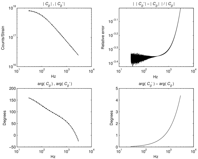
Figure 3: The magnitude (top left) and phase response (bottom left) of the analog sensing function $C_{0}(f)$ (solid curve) and the modified digitised sensing function $C_{0}^{\prime}(f)$ (dotted curve). On the top right the absolute value of the relative error between the two magnitude responses and on the bottom right the difference in degrees of the two phase responses.

Since the quantities in Eqs. (22) and (23) are complex and the measurement contains noise from the external strain the optical gain $\alpha(t)$ has a small imaginary part. This imaginary part is small only to the degree to which Eq. (21) is a good approximation. It should be noted however that Eq. (21) can be made arbitrarily accurate by either making the amplitude of the injected line arbitrarily large or, since the external strain has no component that is correlated with the calibration lines, by integrating for an arbitrarily long amount of time.

The optical gain $\alpha(t)$ is typically calculated on time-scales of a few tens of seconds which, given the typical injected amplitudes of the calibration lines, is sufficient to reduce measurement noise errors to an acceptable few percent.

4 Implementation

4.1 Digitisation of filters and filter performance

The three filters of the feedback loop can be described in terms of analog zero and pole models. This is the starting point of the digitisation procedure.

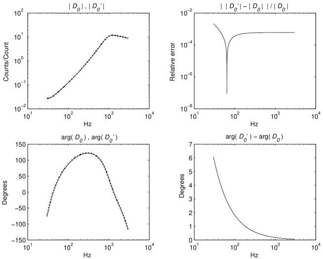
Figure 4: The magnitude (top left) and phase response (bottom left) of the original feedback filter $D_{0}$ (solid curve) and the modified feedback filter $D_{0}^{\prime}$ (dotted curve). On the top right the absolute value of the relative error between the two magnitude responses and on the bottom right the difference in degrees of the two phase responses.

The sensing function $C_{0}$, as we have already discussed, consists essentially of a cavity pole at around $90\,{\rm Hz}$ so the inverse of this filter is a zero at around $90\,{\rm Hz}$. Unfortunately, digitisation of a zero does not lead to a well behaved digital filter. In order to resolve this problem we introduce a pole at high frequencies in the inverted sensing function $C_{0}^{-1}$ prior to digitisation. To ensure the magnitude and phase response of the filter do not change in the frequency range of interest the additional pole is placed at a sufficiently large value of the frequency. We then digitise the analog filter using a bi-linear transform at a sample rate consistent with the presence of the additional pole.

The sensing function also contains a unity gain $8^{\rm th}$ order anti-aliasing elliptic filter at $7570{\rm Hz}$. This filter introduces frequency dependent phase shifts in the data that need to be accounted for. The anti-aliasing filter contains a series of zeros on the imaginary axis, which in the inverted filter turn into poles. To ensure that we obtain a well-behaved inverse digital filter the zeros need to be moved away from the imaginary axis prior to digitisation.

For the Hanford 4km interferometer in the S2 run we generated a modified digital filter $C_{0}^{\prime}$ with a bi-linear transform at a sample rate $16$ times greater than the sample rate the of the time series $q(t)$, i.e. $262144\,{\rm Hz}$. The zeros of the elliptic filter were moved away from the imaginary axis by approximately $160\,{\rm Hz}$ and a single real pole was added at $10^{5}\,{\rm Hz}$.

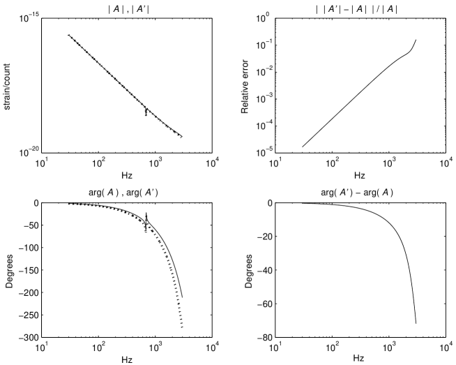
Figure 5: The magnitude (top left) and phase response (bottom left) of the original actuation function $A$ (solid curve) and the modified actuation function $A^{\prime}$ (dotted curve). On the top right the absolute value of the relative error between the two magnitude responses and on the bottom right the difference in degrees of the two phase responses. The large errors in the phase beyond a few hundred Hz are un-important because the contribution to the external strain $h(t)$ from the control signal $x_{c}(t)$ is negligible at these frequencies.

In Figure 3 we show the magnitude and phase responses and errors of the analog sensing function $C_{0}$, as well as our modified digitised sensing function $C_{0}^{\prime}$. The errors between $30{\rm Hz}$ and $3{\rm kHz}$ are less than about $1\%$ in magnitude and $5^{\circ}$ in phase.

The LIGO digital feedback filters $D_{0}$ are constructed from bi-linear transformations at $16384\,{\rm Hz}$ of a series of analog filters. The main one of these is a double pole at DC which, on its own outside a feedback loop, is inherently unstable. In order to stabilise it, the analog filter can be modified by shifting the double pole away from zero by a small amount prior to digitisation. It should be noted that this procedure changes the sign of the feedback filter at DC and introduces errors in the response of the filter at low frequencies. The rest of the filters in $D_{0}$ can be used exactly as they are implemented in the instrument.

Figure 4 shows the magnitude and phase responses, as well as the errors, of the original digital feedback filter $D_{0}$ and the modified digital feedback filter $D_{0}^{\prime}$ for the Hanford 4km interferometer during S2. As expected the errors are larger at low frequencies. However, the errors between $30\,{\rm Hz}$ and $3\,{\rm kHz}$ are less than about $1\%$ in magnitude and $6^{\circ}$ in phase.

The frequency response of the actuation function $A$ is primarily determined by the pendulum suspension of the mirrors and thus consists of a pair of complex poles at the pendulum frequency $f_{p}\approx 0.75{\rm Hz}$. Additionally, the actuation function contains an anti-imaging $4^{\rm th}$ order elliptic filter at $7570{\rm Hz}$, a snubber used to suppress resonances in the electronics and a measured $140\mu s$ time-delay modeled using a $4^{\rm th}$ order Pade filter. The actuator also contains a series of digital notch filters that remove components of the digital control signal at the violin mode frequencies of the mirror suspensions.

All the analog parts of the actuator have been digitised using a bi-linear transform at $16384\,{\rm Hz}$. We have used the existing digital notch filters as they are implemented in the instrument.

Figure 5 shows the result of this procedure. Plotted are the magnitude and phase response of the original actuation function $A$ and the digitised actuation function used in the calibration procedure $A^{\prime}$ as well as the errors for the Hanford 4km interferometer during S2. The errors in the magnitude and phase are less than about $1\%$ and $5^{\circ}$ respectively at frequencies up to a few hundred Hz. At higher frequencies the errors in the phase become larger but this is un-important: the contribution to the external strain $h(t)$ from the control signal $x_{c}(t)$ is negligible above a few hundred Hz.

4.2 Signal processing pipeline

LIGO data is available in so-called “science segments”. At these times the cavities are in resonance and the instrument is sufficiently stable to produce data of scientific quality. The length of science segments depends mostly on the level of seismic activity at the location of each of the sites and can last anywhere between a few tens of seconds to tens of thousands of seconds.

Science runs typically consist of a few hundred science segments. This lends the calculation of the external strain for an entire science run amenable to a cost-effective Beowulf cluster, which is an ensemble of loosely coupled processors with a simple network architecture. In our implementation each processor computes the external strain for a science segment. The few hundred processes required can be scheduled to run on the cluster with a batch system such as Condor [8]. Indeed, the pipeline described below was used to compute the external strain for the entire S2 run for all three LIGO interferometers using Condor on the 300-node Medusa Cluster [9] at UWM.

Figure 6: Signal processing pipeline for time domain calibration. Boxes labeled $\times 16$ and $\times\,1/16$ denote up-sampling and down-sampling respectively.

The first step of our procedure is to compute a table of values for the optical gain $\alpha(t)$ and the digital feedback filter gain $\beta(t)$ for an entire science segment. As we have described in Section 3, obtaining reliable values of the optical gain requires an integration time of a few tens of seconds, so each science segment will have anywhere from a few to a few thousand values of $\alpha(t)$. For the Hanford 4km interferometer during S2 we chose to compute the optical gain every 60s.

Science segments can be up to a few tens of thousands of seconds long. Therefore we cannot keep all the data for a science segment in the memory of a single node. As a result, in our signal processing pipeline, each science segment must be divided into a number of shorter parts. In the current implementation of the pipeline the data is calibrated in $16$ second sub-segments.

Figure 6 shows the digital processing pipeline used in the computation of the external strain $h(t)$ from the error signal, i.e. our implementation of Eq. (16). The top and bottom branches show the computations of the residual and control strains respectively.

To avoid problems involving the dynamic range of double precision floating point numbers, we first high-pass filter 16s of the error signal $q(t)$. For the Hanford 4km interferometer during S2 we implemented the high-pass filter using a $10^{\rm th}$ order Butterworth filter at $40\,{\rm Hz}$. This is a conservative choice and the specific frequency and order of the filter that is necessary depends on the low frequency character of the data. Generally, we expect these choices to depend on the specific science run and interferometer. For numerical stability the high-pass filter is divided into second order sections. Furthermore, to ensure the phase of the signal is not adversely affected by the filtering procedure, the high-pass Butterworth filter is applied to each segment of the data once forward and once in reverse. It should be noted that this procedure is acausal but since we are not attempting to simulate a physical process this is unimportant.

Since the data is being calibrated in segments care must be taken at the boundaries between consecutive segments. The finite impulse response time of the Butterworth filter produces a discontinuity at the beginning and also at the end of each segment (because the high-pass filter is applied forward as well as in reverse). To ensure continuity across contiguous segments we must allow for extra time at the end of each segment. Figure 7 shows a schematic of the procedure we have implemented in the case of three consecutive 16s segments. We use one extra second of data at the end of each segment which allows sufficient time for the high-pass filter to settle. We then then apply the first half of the extra second to the start of the next segment of data. The shaded areas in Figure 7 contain data for which the filters have not settled and are replaced with data from the previous or next segment. It should be noted that this procedure does not remove the few hundred milliseconds of initial ringing of the Butterworth filter at the start of each science segment.

To compute the residual signal $x_{r}(t)$ we first multiply each sample of the high-pass filtered $q(t)$ by a suitably interpolated value of the inverse of the optical gain $\alpha^{-1}(t)$. Interpolations are necessary here because the filter gains are typically computed over a time-scale of tens of seconds, and are not available for every sample of the error signal $q(t)$. We use the table of values of the optical gain created for the entire science segment described above to compute an interpolated $\alpha^{-1}(t)$ for each sample of $q(t)$ using a cubic spline. In principle we could also have used band-limited interpolation but in practice this makes little difference.

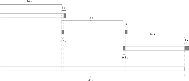
Figure 7: Schematic of three consecutive 16s segments of data. To avoid the discontinuities produced by the finite impulse response of the Butterworth filters in the pipeline, we filter an extra second of data at the end of each 16 s segment. We then use the first half of this second at start of the next segment. Shaded areas contain data for which the filters have not settled and are replaced with data from the previous or next segment.

The inverse sensing function filter has been digitised at $262144\,{\rm Hz}$, and therefore the signal must be up-sampled by a factor of $16$. The up-sampling procedure is simple: $15$ zeros are added between samples and the resulting time-series is smoothed with a low pass filter at a frequency lower than the Nyquist frequency of the original time-series $q(t)$. For the Hanford 4km interferometer during S2 we have chosen a $12^{\rm th}$ order Butterworth filter at $6\,{\rm kHz}$ which is applied to each data segment once forward and once in reverse in second order sections. To ensure continuity across contiguous segments we apply a procedure along the lines described above and in Figure 7 adding an extra second of data at the end of each 16s segment.

We then filter the up-sampled signal through the inverse of the modified sensing function $T_{(C_{0}^{\prime})^{-1}}$. We keep the history of the digital filter across segments to ensure continuity. Finally, to produce the residual signal $x_{r}(t)$ sampled at $16384\,{\rm Hz}$, we down-sample by a factor of $16$ by picking out one out of every $16$ samples.

In our pipeline the digital control signal is computed by multiplying each sample of the high-pass filtered time series $q(t)$ with an interpolated value of the digital filter gain $\beta(t)$ and then filtering the result by the modified digital feedback filter $T_{D_{0}^{\prime}}$. Up to differences between the original and modified digital feedback filter this produces the digital control signal $d(t)$. Note that we could have skipped these steps and instead used the digital control signal that is read out from the instrument.

The low frequency components of $d(t)$ as read out from the instrument and that computed by our pipeline are different. This is mostly due to the high-pass filtering done on $q(t)$ prior to filtering it through $T_{D_{0}^{\prime}}$. In Figure 8 we show a plot of the digital control signal as recorded by the data acquisition system as well as the one computed in our pipeline versus time for a segment of data taken by the Hanford 4 km interferometer during S2. To allow for easier comparison in Figure 8 both the digital control signal as recorded by the data acquisition system and the one produced by our pipeline have been high-pass filtered by applying $4$ second order Butterworth filters at $40\,{\rm Hz}$ consecutively. This removes the low-frequency components and makes the agreement between the two signals manifest.

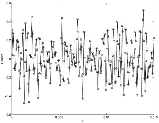
Figure 8: Plot of the digital control signal $d(t)$ as recorded by the data acquisition system (circles joined by a line) and the digital control signal produced by our pipeline (crosses) versus time in seconds for a segment of data taken by the Hanford 4 km interferometer during S2. Due to the high-pass filtering done on the error signal $q(t)$ prior to filtering it through the modified feedback filter $T_{D_{0}^{\prime}}$ the low frequency components of these two signals are different. To allow for easier comparison both signals have been high-pass filtered using $4$ second order Butterworth filters at $40\,{\rm Hz}$.

The digital control signal is then filtered through the modified actuation function $T_{A^{\prime}}$ which produces the control strain $x_{c}(t)$. The histories for both the digital feedback filter $T_{D_{0}^{\prime}}$ and the actuator $T_{A^{\prime}}$ are stored in memory to ensure continuity across 16s segments.

The calibrated strain $h(t)$ is then computed by summing the residual and control strains $x_{r}(t)$ and $x_{c}(t)$.

5 Conclusions

We have described a method to compute the strain $h(t)$ from the output of the LIGO interferometers. This method has been implemented off-line for all three interferometers for the S2 run and results have been presented here for the Hanford 4 km interferometer. The codes that implement the pipeline as well as the digital filters are available under the LSC Algorithm Library (LAL [10]) and the procedure is fully automated under Condor [8].

The pipeline introduces errors associated with the measurement noise involved in the calculation of the optical gain $\alpha(t)$ as well as the digitisation and modifications of the filters. We expect these errors to be less than about $10\%$ in amplitude and $10^{\circ}$ in phase across the detection band. We have tested the pipeline by comparing Fourier transforms of time-domain calibrated data with data calibrated in the frequency domain and found the differences to be well within our errors. We have also faithfully reproduced the digital control signal in the time domain from the error signal using our modified servo filter $T_{G^{\prime}_{0}}$ (see Figure 8).

At this time a third science run (S3) has taken place and a similar off-line procedure will be applied to generate strain data for that run. The current plan is to place an on-line system at the LIGO sites to generate $h(t)$ in the near future.

References

- [1] Abramovici A et al 1992 Science 256 325.
- [2] Barish B and Weiss R 1999 Phys. Today 52 44.
- [3] B. Abbot et al 2004 Nucl.Instrum.Meth. A517 154.
- [4] Adhikari R et al 2003 Class. Quantum Grav. 20 S903; Adhikari R et al 2003 LIGO Technical Note LIGO-T-030097-00-D.
- [5] Wilke et al 2002 Class. Quantum Grav. 19 1377.
- [6] Hewitson M et al 2003 Rev. Sci. Instrum. 74 4184; Hewitson M et al 2003 Class. Quantum Grav. 20 1.
- [7] Mohanty S and Rakhmanov M 2003 LIGO Technical Note LIGO-T-030209-00-Z.
- [8] http://www.cs.wisc.edu/condor/
- [9] http://www.lsc-group.phys.uwm.edu/beowulf/medusa/index.html
- [10] http://www.uwm-lsc.phys.uwm.edu/lal/