On the possible sources of gravitational wave bursts detectable today

Abstract

We discuss the possibility that galactic gravitational wave sources might give burst signals at a rate of several events per year, detectable by state-of-the-art detectors. We are stimulated by the results of the data collected by the EXPLORER and NAUTILUS bar detectors in the 2001 run, which suggest an excess of coincidences between the two detectors, when the resonant bars are orthogonal to the galactic plane. Signals due to the coalescence of galactic compact binaries fulfill the energy requirements but are problematic for lack of known candidates with the necessary merging rate. We examine the limits imposed by galactic dynamics on the mass loss of the Galaxy due to GW emission, and we use them to put constraints also on the GW radiation from exotic objects, like binaries made of primordial black holes. We discuss the possibility that the events are due to GW bursts coming repeatedly from a single or a few compact sources. We examine different possible realizations of this idea, such as accreting neutron stars, strange quark stars, and the highly magnetized neutron stars (“magnetars”) introduced to explain Soft Gamma Repeaters. Various possibilities are excluded or appear very unlikely, while others at present cannot be excluded.

I Introduction

In ref. ROG01 the ROG collaboration has presented the analysis of the data collected by the EXPLORER and NAUTILUS resonant bars during nine months in the year 2001. When the number of coincidences between the two resonant bars is plotted against sidereal time, one finds an excess of events with respect to the expected background, concentrated around sidereal hour four. At this sidereal hour the two bars are oriented perpendicularly to the galactic plane, and therefore their sensitivity for galactic sources of gravitational waves (GWs) is maximal. Furthermore, for these events the energy deposed in one bar is well correlated with the energy deposed in the other. The significance of this observation has been debated  Finn ; ROG02 ; ROG02bis , and certainly further experimental work will be necessary to put the indications on a firmer ground. New data from bars and interferometers, from long data taking runs, should soon clarify the situation.

As we will discuss below, from a theoretical point of view the existence of GW bursts with the intensity and the rate necessary to explain the EXPLORER/NAUTILUS results, if they will be confirmed by further data, would certainly be a great surprise. It would then be necessary to reconsider with an open mind a number of unexpected possibilities. The purpose of this paper is to provide a general framework for such a study, indicating what are the difficulties, which directions of investigation appear to be more promising and which are ruled out. In particular, we hope that our work will help to set the stage for the analysis of future data.

The structure of the paper is as follows. In sect. II we present some of the basic aspects to be explained, that is: (1) the energy which must be released in GWs in order to explain the events observed, and (2) the rate which is inferred from the EXPLORER/NAUTILUS observations. The other crucial experimental information is the distribution of the events as a function of sidereal time. This is presented in sect. III, together with a detailed discussion of what can be learned from sidereal time analysis. We think that this section has also a more general methodological interest. In sect. IV we examine one of the most obvious candidates, the coalescence of a compact binary system. We find that compact objects of solar masses, at typical galactic distances, would account for the energy release. However, the rate expected from binaries made of neutron stars and/or black holes is many order of magnitude smaller than the observed rate. We then turn our attention to more exotic binary systems, such as those involving primordial black holes. The theoretical uncertainties on exotic events make more difficult to put direct limits on their rate. However, the coalescence of binary systems should be a phenomenon which takes place at a more or less steady rate for a time comparable to the age of the Galaxy. We show in sect. V that the corresponding loss of mass of the Galaxy into GWs is constrained by galactic dynamics. Again, we think that this section is of more general interest, independently of the application to the EXPLORER/NAUTILUS data.

These considerations lead us to suggest, in sect. VI, that the all events might be generated by a single (or just a few) “GW burster”, i.e., by an object which emits repeatedly bursts of GWs, and we examine different possible implementations of this idea.

In sect. VII we show that the signal cannot be accounted for by non-gravitational phenomena like the deposition of recoil energy in the bars due to the passage of massive particles. We present our conclusions in sect. VIII.

II Energy requirements

Given a GW with Fourier spectra $\tilde{h}_{+,\times}(f)$, the gravitational energy radiated per unit area and unit frequency is given by Th

$$\frac{dE}{dAdf}=\frac{\pi c^{3}}{2G}f^{2}\left(|\tilde{h}_{+}(f)|^{2}+|\tilde{h}_{\times}(f)|^{2}\right)\,.$$ (1)

For a wave coming from an arbitrary direction and with arbitrary polarization, a detector does not measure directly $\tilde{h}_{+}(f)$ and $\tilde{h}_{\times}(f)$ but rather the combination $\tilde{h}(f)=F_{+}\tilde{h}_{+}(f)+F_{\times}\tilde{h}_{\times}(f)$, where $F_{+,\times}$ are the detector pattern function. For a bar, $F_{+}=\sin^{2}\theta\cos 2\psi$, $F_{\times}=\sin^{2}\theta\sin 2\psi$, where $\psi$ describes the polarizations and $\theta$ is the angle of arrival, measured from the bar axis. The events we consider here are recorded when the bar is orthogonal to the galactic plane, and therefore when $\sin^{2}\theta\simeq 1$. Assuming that the source is emitting randomly polarized GWs, we average over $\psi$. Then

$$\langle\tilde{h}^{2}(f)\rangle\simeq\frac{1}{2}\,\left[|\tilde{h}_{+}(f)|^{2}+|\tilde{h}_{\times}(f)|^{2}\right]\,,$$ (2)

where $\langle\ldots\rangle$ denotes the average over the polarizations and we used $\langle\sin^{2}2\psi\rangle=\langle\cos^{2}2\psi\rangle=1/2$ and $\langle\sin 2\psi\cos 2\psi\rangle=0$. Therefore eq. (1) becomes

$$\frac{dE}{dAdf}=\frac{\pi c^{3}}{G}f^{2}\langle\tilde{h}^{2}(f)\rangle\,.$$ (3)

For a burst, we assume that $\langle\tilde{h}^{2}(f)\rangle$ is equal to a constant $\tilde{h}_{c}^{2}$ between a frequency $f_{\rm min}$ and a frequency $f_{\rm max}$. Denoting by $r$ the distance to the source and assuming isotropic emission, the total radiated energy $\Delta E_{\rm rad}$ is therefore given by

$$\Delta E_{\rm rad}=\frac{4\pi^{2}r^{2}c^{3}\tilde{h}^{2}_{c}}{G}\,\,\frac{1}{3}(f_{\rm max}^{3}-f_{\rm min}^{3})\,.$$ (4)

Typically, the term $f_{\rm min}^{3}$ is negligible in comparison with $f_{\rm max}^{3}$, and therefore we write simply

$$\Delta E_{\rm rad}\simeq\frac{4\pi^{2}r^{2}c^{3}}{3G}\tilde{h}^{2}_{c}\,f_{\rm max}^{3}\,.$$ (5)

For EXPLORER and NAUTILUS the value of $\tilde{h}_{c}$ is related to the energy $E_{s}$ deposed in the bar by

$$\tilde{h}_{c}=2.5\times 10^{-21}\,{\rm Hz}^{-1}\left(\frac{E_{s}}{100\,{\rm mK}}\right)^{1/2}\,\,.$$ (6)

Therefore, under the hypothesis that the events recorded indeed correspond to GWs, each burst originates from a process that liberated in GWs the energy

$$\Delta E_{\rm rad}\simeq 10^{-2}M_{\odot}c^{2}\,\left(\frac{E_{s}}{100\,{\rm mK}}\right)\left(\frac{r}{8\,{\rm kpc}}\right)^{2}\left(\frac{f_{\rm max}}{1{\rm kHz}}\right)^{3}.$$ (7)

A typical value of $E_{s}$ for the considered events is $E_{s}\sim 100$ mK for the 2001 data, see ref. ROG01 .

In terms of the GW amplitude $h$, again assuming a flat Fourier spectrum up to a frequency $f_{\rm max}$, for a burst of duration $\Delta t\simeq 1/f_{\rm max}$ we have $h\simeq\tilde{h}_{c}f_{\rm max}$, so eq. (6) gives

$$h\simeq 2.5\times 10^{-18}\left(\frac{E_{s}}{100\,{\rm mK}}\right)^{1/2}\left(\frac{f_{\rm max}}{1{\rm kHz}}\right)\,.$$ (8)

Assuming that a couple of events are due to backgrounds, as is expected in a two hours period ROG01 , we estimate that the 8 events recorded correspond to a signal rate of order $200$  events/yr. The challenge is therefore to explain what kind of source could give such a strong GW emission, at such a high rate. We also remark that there is no observed neutrino counterpart of these events Aglietta .

III Sidereal time analysis

The other crucial piece of information is the distribution of the number of coincidences when plotted against sidereal time, as stressed in particular in refs. BP1 ; BP2 ; BP3 . The purpose of this section is to discuss in detail what we can learn about the location (and possibly the polarization) of the sources from the sidereal time analysis.

The experimental data for the 2001 run are shown in fig. 1, adapted from ref. ROG01 . The coincidences are binned in one hour bins corresponding to the sidereal hour of arrival. The number of accidental coincidences (dotted line) is estimated shifting the data stream of one detector with respect to the data stream of the other by a step $\delta t=2$ s and measuring the number of coincidences, which now are all accidentals. The analysis is repeated with a step $2\delta t$, then with $3\delta t$, etc., up to $100\delta t$. If $n(j)$ is the number of coincidences found with a shift $j\delta t$, then the average number of accidental coincidences is taken to be $\bar{n}=(1/100)\sum_{j=1}^{100}n(j)$. We see from the figure that there is an excess of coincidences with respect to the expected number of accidentals, at sidereal hours 3 and 4. The data in fig. 1 refers to events collected only in periods with more than 12 hr of continuous operation. If we consider all periods with more than 1 hr of continuous operation the events at the peak becomes $4+4$ rather that $4+3$ as in fig. 1, and the background also rises slightly, see fig. 7 of ref. ROG01 .

Figure 1: The number of coincidences found in the 2001 run (solid line) and the estimated background (dashed line), against sidereal time $\bar{t}=(t_{\rm Expl}+t_{\rm Nau})/2$ (adapted from fig. 5 of ref. ROG01 ).

While the statistical significance of the peak is not large, two important facts make this result more intriguing: (1) sidereal hour 4 is a very special moment. In fact, a peak at this value of sidereal time is predicted to appear for sources in the galactic plane. This is a very general prediction, independent on the precise location and nature of the sources. As we will discuss in detail below, depending on the distribution of sources in the galactic plane (e.g., a uniform distribution in the disk, sources concentrated in the galactic center, etc.) a second peak, possibly smaller, can appear at another value of sidereal time, but the value of $t$ of this second peak depends instead strongly on the specific position of the sources. (2) For the 8 events at the peak, the energy deposed in one bar is very well correlated with the energy deposed in the other, while for the events at other sidereal hours the energy deposed in one bar and in the other are completely uncorrelated ROG01 .

To extract physical informations from the plot against sidereal hour we proceed as follows. Let $\theta$ denote the angle between the direction of a source and the longitudinal axis of the bar. The response of a single bar to GWs from this source is

$$\tilde{h}(f)=\sin^{2}\theta\left(\tilde{h}_{+}\cos 2\psi+\tilde{h}_{\times}\sin 2\psi\right)\,.$$ (9)

Therefore the response in amplitude is proportional to $\sin^{2}\theta$ and, since the energy is quadratic in the amplitude, the response of the detector in energy is proportional to $\sin^{4}\theta$. Furthermore, there can be an effect due to the polarization of the waves, i.e., to the angle $\psi$. We will consider first the case of unpolarized GWs and then we will discuss the possible modification due to the dependence on $\psi$.

III.1 Randomly polarized GWs

If the GWs come from an ensemble of sources or from a single source which emits randomly polarized waves, the effect of $\psi$ will be averaged out and the energy deposed in a detector will just be proportional to $\sin^{4}\theta$. Of course $\theta=\theta(t)$ because of the rotation of the Earth. Using a bit of geometry (whose details are left to appendix A) one can see that

$$\cos\theta(t) = [n_{x}\cos(\alpha-\Omega t)+n_{y}\sin(\alpha-\Omega t)]\cos\delta+$$ (10)

$$+n_{z}\sin\delta\,,$$

where $\alpha,\delta$ are the right ascension and declination of the source, $a$ is the azimuth of the bar, $l$ its latitude, $n_{x}=-\cos a\sin l$, $n_{y}=\sin a$, $n_{z}=\cos a\cos l$, $\Omega=2\pi/24$ is the rotation frequency of the Earth in units $1/$ (sidereal hours), $t$ is the local time measured in sidereal hours, and all angles, including $\alpha,\delta$, are expressed in radians.

The axis of the two detectors are aligned to within a few degrees of one another, so that the response of the two bars to any source can be considered identical. The latitudes and azimuths are: for EXPLORER, $l=46.45N$ and $a=39^{o}E$ while for NAUTILUS $l=41.82N$, $a=44^{o}E$. The longitudes are instead $6.20E$ and $12.67E$, respectively. Given their difference in longitude, the local sidereal time at the EXPLORER and at the NAUTILUS locations differ by $\Delta t\simeq 25.88$ min. We will denote by $\bar{t}$ the average between the two local sidereal times, $\bar{t}=(t_{\rm Expl}+t_{\rm Nau})/2\simeq t_{\rm Expl}+0.216$ hr. (The same variable was used in ref. ROG01 . To compare with other experiments it might be more convenient to use Greenwich sidereal time $t_{\rm Green}$, related to $\bar{t}$ by $\bar{t}\simeq t_{\rm Green}+0.629$ hr).

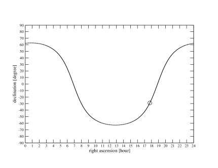
Figure 2: The location of the galactic plane in the equatorial coordinate system. The position of the galactic center is marked by a circle.

In the equatorial coordinate system $(\alpha,\delta)$ the galactic plane is represented by the curve in fig. 2. For sources in the galactic plane a plot of $\sin^{4}\theta$ against sidereal time $t$, with $0\leq t\leq 24$, always shows two maxima: one peak is close to sidereal hour 4, because at that moment the bar turns out to be almost perpendicular to the galactic plane. The precise position of the source within the galactic plane results only in a minor variation of the precise value of $\bar{t}\simeq 4$ where $\sin^{2}\theta=1$. Instead, the sidereal time at which there is the second peak depends strongly on the location of the source.

Fig. 3 shows $\sin^{4}\theta$ as a function of $\bar{t}$ for a source located in the galactic center, i.e., $\alpha=266.405^{o}$ and $\delta=-28.936^{o}$. In fig. 4 we show $\sin^{4}\theta$ for another source in the galactic plane, taking as an example a source with equatorial coordinates $(\alpha=135^{o},\delta=-40^{o})$. Both curves have a maximum in the bin $4<\bar{t}<5$ (more precisely, at $\bar{t}\simeq 4.55$ for the galactic center and $\bar{t}\simeq 4.27$ for the source of fig. 4) and they have a second peak whose position depends on the source location. Furthermore, they have a minimum where $\sin^{4}\theta$ becomes zero. Moving away from the galactic plane, e.g. increasing the declination $\delta$ at fixed $\alpha$ (see fig. 2) at first the curve still has two maxima, with positions that depend on the values of $(\alpha,\delta)$, but then one arrives at a critical value of $\delta$ where the two maxima coalesce. Above this critical value there is just a single maximum, and as we increase further $\delta$ the value at the peak becomes smaller than one. At the same time the value at the minimum moves away from zero, and therefore the response curve becomes much flatter. Fig. 5 shows the curve for a source with $\alpha=266.405^{o},\delta=80^{o}$. In the limit $\delta=90^{o}$ we see from eq. (10) that the curve becomes flat, at a value which depends on $a,l$, and which in our case is $\sin^{4}\theta\simeq 0.504$. A plot of $\sin^{2}\theta$ as a function of the local sidereal time $t$ and of the declination $\delta$ is shown in fig. 6. The effect of changing $\alpha$ on this figure is simply to produce a shift in the origin of sidereal time, as we see from the fact that in eq. (10) $\alpha$ and $t$ appear only in the combination $\alpha-\Omega t$.

Figure 3: $\sin^{4}\theta$ against sidereal time $\bar{t}$ (in hr) for the galactic center.

Figure 4: $\sin^{4}\theta$ against sidereal time $\bar{t}$ (in hr) for a source with coordinates $\alpha=135^{o}$ and $\delta=-40^{o}$.

Figure 5: $\sin^{4}\theta$ against sidereal time $\bar{t}$ (in hr) for a source with $\alpha=266.405^{o},\delta=80^{o}$.

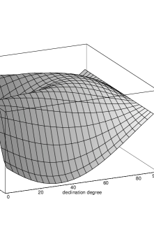
Figure 6: $\sin^{2}\theta$ as a function of sidereal time $t$ and of the declination $\delta$, for $\alpha=135^{o}$.

We now discuss how these response curves are reflected in a plot of the number of observed coincidences, $N_{c}$, against sidereal time. Consider for definiteness the situation in which the sources are in the direction of the galactic center. In fig. 3 we have shown $\sin^{4}\theta$ as a function of $\bar{t}$ for these sources, and it is intuitive that the maxima of $N_{c}$, as a function of $\bar{t}$, coincide with the two maxima of $\sin^{4}\theta$, since at that values of sidereal time the bars have their best orientation with respect to these sources. However, it is important to understand that the functional form of $N_{c}$, and in particular the width of the maxima, is not the same as that of the function $\sin^{4}\theta$. Rather, it depends crucially on the ratio between the energy of the events and the energy threshold of the detectors BP1 ; BP2 ; BP3 ; ROG02bis . To understand this point, suppose that in a given observation time arrive $n$ events in each one-hour bin and restrict for the moment to the simplified situation in which a signal arriving at a generic sidereal time $t$ deposes in the bar an energy $E_{0}\sin^{4}\theta(t)$, with $E_{0}$ the same for all signals. Consider first the limiting case in which the threshold of the detector is very low with respect to $E_{0}$, e.g., is represented by the dotted line $A$ in fig. 7. In this case all the events are above threshold and therefore are recorded, except those falling exactly in the blind direction of the detectors, which in this example corresponds to the bins between sidereal hours 19 and 23. Therefore in the bins corresponding to sidereal hours 19 to 23 we would record zero events, while in all others we would observe $n$ events per bin. In this limiting case, therefore, $N_{c}(\bar{t})$ shows no peak at all; rather, it is a flat function, $N_{c}(\bar{t})=n$, except for a dip in correspondence to the blind direction.

The opposite limiting case is represented by an energy threshold very close to $E_{0}$ (the dotted line B in fig. 7). In this case, only when we are in the two bins where $\sin^{4}\theta$ becomes equal to one we can detect the signals, while as soon as we move to the next bin we fall below the threshold and no signal is detected. In this case $N_{c}=n$ in the bins $4<\bar{t}<5$ and $13<\bar{t}<14$, while $N_{c}=0$ otherwise. A plot of $N_{c}(\bar{t})$ will show two very narrow peaks, each one concentrated just in a single sidereal hour bin.

In a more realistic situation, the above picture will be complicated by the fact that the signals will arrive with a distribution in energy, rather than being monoenergetic. Moreover, the energy of the events is in any case “dispersed” by the fact that the events observed are a combination of the GW signal and of the noise. The above example, however, suffices to illustrate that the width of the peak is crucially affected by the energy distribution of the events and by the detector thresholds, and can be very flat (for great values of the typical signal-to-noise ratio) to very narrow (for small SNR). One should also observe that, when the average SNR of the events is small, we can see $\sin^{4}\theta$ as a measure of the probability that, in a single detector, a signal is not lost below the energy threshold. In a two-detector correlation the probability that both detectors see the signal is therefore rather measured by $\sin^{8}\theta$, which therefore is a more appropriate envelope for the graph in fig. 7, and this results in an even narrower peak.

It is also interesting to note that, in the case of large SNR, informations on the location of the sources cannot be extracted from $N_{c}(t)$, which is now basically flat, but it could be obtained plotting against sidereal time the average energy of the coincident events, although probably a large sample of data would be needed, to compensate for the spread in the intrinsic energies of the signals.

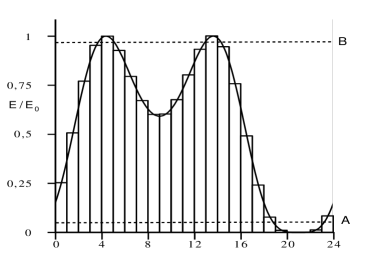
Figure 7: The energy of the events in the various sidereal time bins, compared to two possible thresholds of the detectors (the dotted lines marked as A and B).

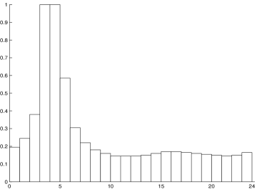
Figure 8: A simulation of the number of events per bin, for a distribution of sources in the galactic plane (chosen to be uniform in galactic longitude) when the detector threshold is such that $E/E_{0}=0.9$.

If we assume a given distribution of sources and a given typical value of the detector threshold with respect to the signal, we can simulate the distribution of the number of events as a function of sidereal time. In fig. 8 we show an example where, for illustration, we considered a population of sources all in the galactic plane, and distributed uniformly in galactic longitude (this is natural for sources seen from the Earth, if we can detect only sources which are not too far, say $r<0.5$ kpc. If one would be sensible also to very far sources, then clearly toward the galactic center there would be many more sources than in the opposite direction). We assume that each source deposit in the bar an energy $E_{0}\sin^{4}\theta(t)$, with $E_{0}$ the same for all bursts and for all sources. We fix a detector threshold (in fig. 8 we have chosen a rather high threshold, $E/E_{0}=0.9$). For each source we produce a plot as fig. 7, and we see which bins are above threshold. Then as the contribution of this source we take $N_{c}(t)=1$ for these bins and $N_{c}(t)=0$ otherwise. Summing the contributions of all sources and normalizing the distribution so that the value at the peak is one, we get fig. 8. Of course this is a rather simplified model, but it illustrates that a distribution of galactic sources may produce a single peak close to sidereal hour four (whose width is controlled by the threshold that we set).

Comparing with the experimental data in fig. 1 we see that the preliminary indication, within the statistics available, is that there could indeed be a peak near sidereal hour 4. No second peak of some statistical significance can be seen. From the above discussion, this points toward the existence of several sources distributed across the galactic disk. Independently of the details of the models considered in fig. 8, the result follows more generally from the fact that for a distribution of sources in the galactic plane each single source would contribute either to the bins around sidereal hour 4 common to all sources in the galactic plane, or to another bin which depends on the specific source location. Only in the former case the contributions from different sources add up and, within the present statistics, give rise to something which emerges over the background.

However, here we should not rush toward conclusions. Even assuming that the events really correspond to GWs, it is clear that the full form of the curve can be understood only when sufficient statistics will be available. We will therefore keep open, for the moment, the possibility that further structures in the sidereal time plot might appear with further data, and we will examine different possibilities.

We also mention that the sidereal time analysis can be very useful even in the study of extragalactic sources BP1 ; BP2 . However, eq. (7) clearly excludes an interpretation in terms of GWs of extragalactic origin for the EXPLORER/NAUTILUS data, and therefore we will focus on galactic sources.

III.2 Polarized GWs

In sect. VI we will examine the possibility that all events come from just one source which emits repeatedly GW bursts. One can expect from such a source a coherent motion of matter with some given quadrupolar pattern related to the source geometry and to its rotation axes, and consequently the emission of polarized GWs. As we will see in this section, the polarization can affect the sidereal time analysis in an interesting way.

The response of the detector (in amplitude) is given in eq. (9), and the polarization angle $\psi$ depends on sidereal time, just as $\theta$. The calculation of the dependence of this response function on local sidereal time $t$, for a given location of the source and a given choice of the polarization axes, is in principle straightforward but somewhat lengthy, and we give the details in Appendix A.

In fig. 9 we show the result for a source located in the direction of the galactic center (a similar result is reported in ref. BGMP ). In this figure the envelope is $\sin^{4}\theta$, i.e. the response function (in energy) for an unpolarized source, and is therefore the same quantity already shown in fig. 3. The thick line is the function $\sin^{4}\theta\cos^{2}2\psi$, i.e. the response function (in energy) for a source which has only the $+$ polarization, while the dotted curve is $\sin^{4}\theta\sin^{2}2\psi$, i.e. the response function in energy for the $\times$ polarization. (The angle $\psi$ is measured with respect to an axis orthogonal to the propagation direction and lying along the galactic plane, see Appendix A).

Figure 9: The response function in energy for unpolarized GWs (the envelope), for the $+$ polarization (thick line), and for the $\times$ polarization (dotted line), for a source at the Galactic center.

From this figure we see a number of interesting effects. First of all, the maxima are shifted with respect to the unpolarized case. This is due to the fact that the maxima of $\sin^{2}2\psi$ and of $\cos^{2}2\psi$ do not coincide in general with the maxima of $\sin^{4}\theta$, and therefore the position of the peaks in the response function is determined by a combination of the two effects. For the same reason, the values of the response function at the peaks will be smaller than one, and need not be equal among the two peaks. We also see that the peak close to sidereal hour 4 in the $+$ polarization is narrower compared to the unpolarized case, because for the $+$ polarization the maximum of $\cos^{2}2\psi$ is close to the maximum of $\sin^{4}\theta$ (as we see from the fact that the position of the peak close to sidereal hour 4 is only slightly shifted) and therefore the additional factor $\cos^{2}2\psi$ in the energy response gives a further suppression outside the peak. New blind directions appear, when $\cos^{2}2\psi=0$ or $\sin^{2}2\psi=0$, which contribute to make the peaks narrower.

Figure 10: The square of the quantities shown in fig. 9 (which is the appropriate response function for a two-detector correlation).

Recalling that the response function of a two-detector correlation, for low typical SNR, is the square of the single-detector response function, we see that finally we can obtain very narrow peaks, as shown in fig. 10. This means that in the case of a source emitting waves with a high degree of polarization along the galactic plane it is not necessary to have a very low value of the typical SNR in order to find a narrow peak in the number of observed coincidences $N_{c}(\bar{t})$. A threshold of order $0.5$ in the response function of fig. 10 suffices to have $N_{c}(\bar{t})$ concentrated in just two hour bins around $\bar{t}=4$, for a source radiating the $+$ polarization. Therefore the number of observed events is not necessarily a large underestimate of the total number of events, as it would instead be the case if most of the signals were lost below the threshold.

In this example we have considered the (rather special) case in which the $+$ polarization is perpendicular to the galactic plane, i.e., the two axes used to define $h_{+}$ and $h_{\times}$ are one parallel and the other perpendicular to the galactic plane (see Appendix A). More in general, we can rotate these axes in the transverse plane by an angle $\psi_{0}$. A source which, with respect to these new axes, emits purely the $h_{+}$ (or purely the $h_{\times}$) polarization will have a response function obtained shifting $\psi\rightarrow\psi-\psi_{0}$, and therefore the position of the peaks depends on $\psi_{0}$. As an example, we show in fig. 11 the response to the $+$ and $\times$ polarization, for a source located at $\alpha=135^{o},\delta=-40^{o}$ (i.e., the same source as in fig. 4) and with $\psi_{0}=0.25$ rad.

Figure 11: The same as fig. 9, for a source with coordinates $\alpha=135^{o},\delta=-40^{o}$, and with a shift $\psi\rightarrow\psi-\psi_{0}$ with $\psi_{0}=0.25$ rad.

IV Coalescence of compact binaries

As we will recall below, for binaries with neutron stars (NS) and/or black holes (BH) the expected galactic merging rates are far too small, compared to the value $O(200)$ events per year discussed in sect. II. However, stimulated by the experimental data, one might wish to consider more unusual possibilities, like BHs of primordial origin or other exotic objects. For this reason, and also in order to understand better the difficulties of finding a good candidate source for the EXPLORER/NAUTILUS data, we start our discussion with the coalescence of compact binaries.

The merging of NS-NS, NS-BH or BH-BH binaries is a process that generates GWs at the kHz, where the bars are sensitive. Furthermore, they typically liberate an energy of order $10^{-2}M_{\odot}c^{2}$ in GWs. This can be estimated first of all analytically, using the wave form of the inspiral phase,

$$h_{+}(t) = -\frac{2^{4/3}}{r}(GM_{c})^{5/3}\omega_{\rm gw}^{2/3}(\tau)\,\left(\frac{1+\cos^{2}\iota}{2}\right)\cos[\Phi(\tau)]\,,$$

$$h_{\times}(t) = -\frac{2^{4/3}}{r}(GM_{c})^{5/3}\omega_{\rm gw}^{2/3}(\tau)\,\cos\iota\,\sin[\Phi(\tau)]\,,$$ (11)

where $M_{c}$ is the chirp mass, $M_{c}=(M_{1}M_{2})^{3/5}/(M_{1}+M_{2})^{1/5}$, $M_{1},M_{2}$ are the masses of the two objects, $\iota$ is the inclination of the orbit with respect to the line of sight, $\tau$ is the time to coalescence, $\Phi$ is the accumulated phase and $\omega_{\rm gw}(\tau)$ is the chirping frequency of the GW. Explicitly,

$$\Phi(t)=\frac{8}{5}\left(\frac{5^{3/8}}{4}\right)(GM_{c})^{-5/8}\tau^{5/8}+\Phi_{0}\,,$$ (12)

$$\omega_{\rm gw}(\tau)=\left(\frac{5^{3/8}}{4}\right)(GM_{c})^{-5/8}\tau^{-3/8}\,.$$ (13)

Taking the Fourier transform in the saddle point approximation (see e.g. ref. Cut ) one gets, apart from irrelevant phases,

$$\tilde{h}_{+}(f) = \frac{1}{\pi^{2/3}}\,\left(\frac{5}{24}\right)^{1/2}\frac{1}{r}\frac{(GM_{c})^{5/6}}{f^{7/6}}\,\left(\frac{1+\cos^{2}\iota}{2}\right)\,,$$

$$\tilde{h}_{\times}(f) = \frac{1}{\pi^{2/3}}\,\left(\frac{5}{24}\right)^{1/2}\frac{1}{r}\frac{(GM_{c})^{5/6}}{f^{7/6}}\,\cos\iota\,.$$ (14)

Using eq. (1) and performing the angular integration one finds the energy spectrum,

$$\frac{dE}{df}=\frac{\pi^{2/3}}{3G}\,(GM_{c})^{5/3}\,f^{-1/3}\,.$$ (15)

Integrating up to a maximum frequency $f_{\rm max}$ for which we are still in the inspiral phase we can estimate the total energy radiated during the inspiral phase,

$$\Delta E_{\rm rad}\simeq\frac{\pi^{2/3}}{2G}(GM_{c})^{5/3}\,f_{\rm max}^{2/3}\,,$$ (16)

or, inserting the numerical values,

$$\Delta E_{\rm rad}\simeq 4.2\times 10^{-2}M_{\odot}c^{2}\,\left(\frac{M_{c}}{1.22M_{\odot}}\right)^{5/3}\,\left(\frac{f_{\rm max}}{1\,{\rm kHz}}\right)^{2/3}\,,$$ (17)

where the normalization of the chirp mass corresponds to $M_{1}=M_{2}=1.4M_{\odot}$.

This simple analytic treatment gives a value in very good agreement with that found numerically, from sophisticated hydrodynamical simulations of NS-NS coalescence including both the inspiral and plunge phases Ruf ,

$$\Delta E_{\rm rad}\simeq(1-3)\times 10^{-2}\,M_{\odot}c^{2}\,.$$ (18)

Figure 12: The distribution of distances $r$ against mass $M$ for the eight 2001 events at the peak at sidereal hours 3 and 4.

Figure 13: The distribution of distances $r$ against $\cos\iota$ for the eight 2001 events at the peak at sidereal hours 3 and 4, setting $M=1.35M_{\odot}$.

Comparison with eq. (7) indicates that, from the energetic point of view, the coalescence of compact binaries is an interesting candidate. Actually, eq. (7) has been obtained assuming, for lack of better informations, a square waveform in frequency space. Since in the case of an inspiral we have the exact waveform, we can be more precise. Averaging over the angle $\psi$ we have in fact

$$\tilde{h}_{c}^{2}=\frac{1}{2}\sin^{4}\theta\left(|\tilde{h}_{+}(f)|^{2}+|\tilde{h}_{\times}(f)|^{2}\right)\,,$$ (19)

while from eq. (14) we have

$$|\tilde{h}_{+}(f)|^{2}+|\tilde{h}_{\times}(f)|^{2}=\frac{5}{24\,\pi^{4/3}r^{2}}\frac{(GM_{c})^{5/3}}{f^{7/3}}\,g(\iota)\,,$$ (20)

where

$$g(\iota)=\left(\frac{1+\cos^{2}\iota}{2}\right)^{2}+\cos^{2}\iota\,.$$ (21)

We can then substitute this expression for $\tilde{h}_{c}$ into eq. (6). We set $f\simeq 920$ Hz (corresponding to the resonant frequency of the bars). For events coming from the galactic plane, detected around sidereal hour four, we can also set $\sin\theta\simeq 1$. Then we find

$$\frac{E_{s}}{100\,{\rm mK}}\simeq 1.1\,\left(\frac{M_{c}}{1.22M_{\odot}}\right)^{5/3}\,\left(\frac{8\,{\rm kpc}}{r}\right)^{2}\,\left(\frac{g(\iota)}{0.8}\right)\,.$$ (22)

We have chosen as a reference value for $g(\iota)$ its average value over the solid angle. Each event, i.e. each value of $E_{s}$, determines a curve in the plane $(\tilde{M}_{c},r)$, where

$$\tilde{M}_{c}=M_{c}\,\left(\frac{g(\iota)}{0.8}\right)^{3/5}$$ (23)

and this allows us to check whether each event can be interpreted with reasonable values for $M_{c}$ and $r$. The function $g(\iota)$ varies between between $1/4$ for $\cos\iota=0$, i.e. when the observer is in the plane of the orbit, and $g(\iota)=2$ for $\cos\iota=1$, i.e. when the line of sight of the observer is perpendicular to plane of the orbit. Correspondingly, $\tilde{M}_{c}$ ranges between $0.50M_{c}$ and $1.73M_{c}$.

The results are shown in fig. 12, for the eight events at sidereal hours 3 and 4 in the 2001 data. We have written $M_{c}=M/2^{1/5}$, which is the chirp mass of a system with two equal masses $M_{1}=M_{2}=M$, and we have fixed $g(\iota)=0.8$. In fig. 13 we fix instead $M=1.35M_{\odot}$, a typical value for a NS, and we plot $r$ against $\cos\iota$ for the same eight events.

We see that very natural values of $M$ and $r$ are obtained. Binary systems composed of compact solar-mass objects, at typical galactic distances, would be compatible with the energetic observed in the events.

The problem with these sources, however, is the rate. Before the recent discovery of a new NS-NS binary, the rate of NS-NS coalescences in the Galaxy was estimated to be in the range $10^{-6}$ to $5\times 10^{-4}$ mergings per year KNST . This estimate depends strongly on the shortest-lived systems known, and the recent discovery of a new NS-NS binary, with the shortest known merging time (85 Myr), brings this estimate up by one order of magnitude, possibly up to a factor 30 Bur ; still, we are very far from the $O(200)$ events per year needed to explain the NAUTILUS/EXPLORER observations. The estimates of the coalescence rate of binary systems involving black holes (BH-BH and BH-NS) can be based only on stellar evolution models, rather than on observations, since no such systems have yet been observed. The theoretical calculations suffers from large uncertainties, but the rate for BH-BH and BH-NS coalescence is estimated to be of the same order of magnitude (or smaller) than the NS-NS coalescence rate, see e.g. ref. BKB and references therein.

Under the stimulus of the NAUTILUS/EXPLORER data, one might consider more exotic possibilities, as for example black hole of primordial rather than astrophysical origin. In this case the estimates based on stellar evolution do not apply, and it is interesting to observe that primordial BHs produced in the early universe at the QCD phase transition would have today a mass of approximately $0.5M_{\odot}$ Jed . The density of MACHO’s, and therefore also of primordial BHs of mass $\sim 0.5M_{\odot}$, can be constrained from the microlensing of stars from the Large Magellanic Cloud Alc ; Benn . These data suggest that the fraction of our Galaxy’s stellar mass which is in the form of black holes can be significantly larger than 1%. With some assumptions, the fraction of primordial black holes in binary systems, and their distributions in eccentricity and semi-major axis has been estimated in NakTh ; Nak , and it has been found that the coalescence rate of primordial black hole binaries could be of order $5\times 10^{-2}$ events per year per galaxy. This is still far too small to explain the data. Furthermore, a stellar population of primordial origin is expected to reside in the galactic halo rather than in the galactic disk, so there should be no reason to get an enhanced signal when the bars are oriented favorably with respect to the galactic plane. However, when one enters into the realm of exotic possibilities there are large uncertainties in the theoretical estimates. For instance, for primordial black holes, there are large uncertainties on the detailed formation mechanism, and therefore one should keep an open mind on this option.

Other interesting informations might come observing that the coalescence of any population of compact binaries should be a phenomenon which takes place at a more or less steady rate for a timescale comparable to the age of the Galaxy. It is therefore useful to examine whether, independently of the nature of the sources, the corresponding mass loss of the Galaxy to GWs is compatible with known facts of galactic dynamics. We discuss this issue in the next section.

V Upper limits on the GW emission from the Galaxy

From the energy radiated in each burst, eq. (7), and a rate $O(200)$ events/yr, we see that the mass lost by the Galaxy into GWs is of order

$$-\dot{M}\sim 2\frac{M_{\odot}}{\rm yr}\,\left(\frac{r}{8\,{\rm kpc}}\right)^{2}\left(\frac{f_{\rm max}}{1{\rm kHz}}\right)^{3}\,,$$ (24)

where now $r$ is an average distance of these sources. If the events are indeed due to the merging of compact objects we know the energy which has been released by each burst, independently of the values of $r$ and of $f_{\rm max}$, see eq. (18), and therefore we can write

$$-\dot{M}\sim(2-6)\frac{M_{\odot}}{\rm yr}\,.$$ (25)

This is a very large mass loss. For comparison, the mass loss of the Galaxy due to electromagnetic radiation is $9\times 10^{-3}M_{\odot}/{\rm yr}$. In this section we will investigate whether such a high value is compatible with known facts of galactic dynamics.

If the mass loss is really due to GWs from a number of different sources distributed across the galactic disk, it is difficult to imagine that its rate changed dramatically with time over the age of the Galaxy. Assuming a steady mass loss at the level of eq. (25) for a time comparable to the age of the oldest clusters in the Galaxy, $T\sim 1.2\times 10^{10}$ yr, gives a total mass loss over the history of the Galaxy of at least $\Delta M\sim 2\times 10^{10}M_{\odot}$. For comparison, the total mass of the disk is estimated to be $6\times 10^{10}M_{\odot}$ and the total mass of the disk plus bulge and spheroid is $9\times 10^{10}M_{\odot}$. The total halo mass is $M_{\rm halo}\sim 2\times 10^{12}M_{\odot}$ WE , but for us this is a less relevant reference value, since this is the mass in a spherical halo with radius of order 170 kpc, and therefore events coming from the halo would not show any special correlation with the galactic plane.

Of course, the present value of the mass of the Galaxy gives only a first scale for comparison, since on the one hand we can imagine that the mass of the Galaxy could have been larger at the formation and, on the other hand, tighter constraints on the possible mass loss may come from galactic dynamics. Some of these issues have been considered many years ago SFR ; PA ; OB , and it is interesting to go back to these considerations using the present knowledge of galactic dynamics, and to compare with the energy loss given in eq. (25). The most stringent limits are discussed in the following subsections.

V.1 Effect of the mass loss on the radial velocity of stars

Let us first recall the basic fact of galactic dynamics that, because of the differential rotation of the Galaxy, the radial velocities $v_{r}$ of stars as seen from the sun, at first order in the distance $R$ between the sun and the star (after correcting for the solar motion and averaging over the peculiar velocities of the individual stars) is given by

$$v_{r}=AR\sin 2l\,,$$ (26)

where $A=(-1/2)(Rd\omega/dR)_{\odot}$ is Oort’s $A$ constant, $l$ is the galactic longitude, and for simplicity we have written only the expression valid for galactic latitude $b=0$ (see e.g. BT ).

If the Galaxy is loosing mass, stars become less and less bound and acquire radial velocities with respect to the Galaxy rest frame. The physics of the effect can be understood easily limiting ourselves to a star in a circular orbit of radius $r$ in the galactic plane, with a Keplerian longitudinal velocity $v_{l}$ given by $v_{l}^{2}=GM/r$; $M$ is an effective mass related to the mass at the interior of $r$. In particular the effective mass inside the solar circle is obtained from $v_{l}\simeq 220$ km/s and $r\simeq 8$ kpc and is $M\simeq 8\times 10^{10}M_{\odot}$. The conservation of the angular momentum $J=mrv_{l}$ gives $\dot{r}v_{l}+r\dot{v}_{l}=0$, or $v_{r}/r=-\dot{v}_{l}/v_{l}$, where $v_{r}=\dot{r}$ is the radial velocity in the frame of the Galaxy. Using the Keplerian value for $v_{l}$, this gives

$$v_{r}=-\frac{\dot{M}}{M}\,r\,.$$ (27)

In the frame of the sun, this gives an additional contribution to the radial velocity (26),

$$v_{r}=AR\sin 2l+KR\,,$$ (28)

where

$$K=-\frac{\dot{M}}{M}\,.$$ (29)

and $R$ is the sun-star distance. In the literature on galactic dynamics the additional term in eq. (28) is known as a K-term. (More generally, one can define a K-term as any additional term to be added to the right-hand side of eq. (26), independent of the galactic longitude, and with an arbitrary dependence on $R$, e.g. a constant. We see that in the case of mass loss one gets a K-term growing linearly with $R$). The difficulty of extracting from the data the effect due to the mass loss is that the K term receives contributions from many other effects of galactic dynamics; for example, the value of $K$ extracted from young stars at distances $R<0.6$ kpc is strongly influenced by the kinematic peculiarities of the Gould Belt, and therefore the value of $K$ depends on the distance of the sample, and it turns out to depend also on the age of the stars chosen. To have an idea of the systematics involved, we observe that ref. TFF , using the Hipparcos data, finds that for $0.1{\rm kpc}\leq R\leq 0.6$ kpc, $K$ (expressed in km/(s kpc) ) ranges from $7.1\pm 1.4$ if one uses stars younger than 30 Myr to $-5.4\pm 2.3$ for stars with age between 60-90 Myr, with an average over all stellar ages $K=0.5\pm 0.9$. Samples including only stars at larger distances, and therefore insensitive to the Gould belt, give instead negative values of $K$; in particular, including only stars with $0.6{~{}\rm kpc}\leq R\leq 2$ kpc, and averaging over all stellar ages, one finds $K=-2.9\pm 0.6$ TFF . A negative value of $K$ might in principle be due to the influence of the spiral arm structure, but even taking into account spiral arm kinematics, the sample at $R>0.6$ kpc gives a negative value, $K=-(1-3)\,{\rm km}\,\,{\rm s}^{-1}\,{\rm kpc}^{-1}$ FFT , and the physical origin of the negative sign, representing a contraction rather than an expansion, is not really well understood.

To get a bound on the energy loss to GWs, one should in principle be able first of all to understand the other mechanisms which are at work and which give a negative contribution to $K$, evaluate them precisely, subtract them, and see if one is left with a positive value of $K$ growing linearly with $R$. This is beyond the accuracy of our knowledge of the Galaxy. However, in any case we certainly do not expect a fine tuned cancellation between some negative contributions to $K$ and the positive contribution due to a possible GW emission. Let us assume for definiteness that a positive contribution to $K$ from GW mass loss is smaller than 20% of the absolute value of $K$. We use the value measured at $R>0.6$ kpc, to get rid of effects due to the Gould Belt, i.e., $K=-(1-3)\,{\rm km}\,\,{\rm s}^{-1}\,{\rm kpc}^{-1}$, and therefore we assume that the positive contribution from GWs is smaller than $O(0.4)\,{\rm km}\,{\rm s}^{-1}\,{\rm kpc}^{-1}$. From eq. (29), using $M=8\times 10^{10}M_{\odot}$, this translates into

$$-\dot{M}<O(30)M_{\odot}/{\rm yr}\,.$$ (30)

Clearly, the precise value of the bound can be modified somehow, changing the level of fine tuning that one is willing to tolerate, but eq. (30) gives a first order-of-magnitude estimate.

V.2 Mass loss and outward motion of the LSR

Rather than looking at the $K$ term, i.e. at the expansion/contraction of the stars within a few kpc from the sun, one can investigate whether the local standard of rest (LSR) has an overall outward radial velocity, as suggested by eq. (27). Long ago Kerr Kerr indeed suggested an outward radial motion of the LSR with a velocity $u_{\rm LSR}=7$ km/s, as an explanation for the lack of axisymmetry of the galactic rotation curve obtained with 21 cm surveys, and this effect was attributed to mass loss due to GWs in ref. SFR . In more recent years the experimental determination of $u_{\rm LSR}$ has not become much more clear. Blitz and Spergel BS from 21 cm line emission find $u_{\rm LSR}=+14$ km/s (where the positive sign means radially outward); results consistent with this value have been found from Cepheid kinematics MCS while in ref. KT , from a variety of measurements (OH/IR stars, globular clusters, high-velocity stars, planetary nebulae), it is proposed $u_{\rm LSR}=-1\pm 9$ km/s. From young open clusters Hron one finds a maximum value $u_{\rm LSR}=3\pm 2$ km/s. Recent work on OH/IR stars DGS gives $u_{\rm LSR}=2.7\pm 6.8$ km/s.

However, even if an outward velocity of the LSR of a few km/s indeed exists, it cannot be due to mass loss. In fact, the observation of the 21 cm absorption line toward the galactic center RS shows that the gas along the line-of-sight has a mean radial velocity with respect to the LSR of $-0.23\pm 0.06$ km/s. The absorbing material is probably at 1-2 kpc from the galactic center. A radial expansion due to mass loss predicts a radial velocity $v_{r}\sim r$, eq. (27), and therefore, if at the sun location $r\simeq 8$ kpc this effect has to be responsible for a velocity of the LSR, we should see a comparable difference in velocity between us and this gas, $\Delta v_{r}=(-\dot{M}/M)\Delta r$. The model of Blitz and Spergel based on the existence of a rotating triaxial spheroid BS manages to escape this limit because it predicts a dependence of $v_{r}$ on $r$ rather flat between 3 and 8 kpc from the galactic center. For a mass-loss model instead $v_{r}\sim r$ and we do not have this escape route.

As in the previous section, there can be in general both positive and negative contributions from different physical mechanisms to the value $\Delta v_{r}=-0.23\pm 0.06$ km/s, and to extract a bound on mass loss to GW (or, for that matter, to any mass loss) we require that no fine tuning between different contributions takes place. Again we set conventionally at 20% the maximum fine tuning that we allow, which means that we say that a positive contribution from GWs to $\Delta v_{r}$, if it exists at all, must be smaller than $O(0.04)$ km/s. Setting the distance between us and the gas to $\Delta r=6$ kpc, this gives a bound on the mass loss to GWs, $(-\dot{M})/{M}<O(0.04)\,{\rm km}\,{\rm s}^{-1}/{6\,{\rm kpc}}$; using again $M=8\times 10^{10}$, this means

$$-\dot{M}<O(0.5)\,M_{\odot}/{\rm yr}\,.$$ (31)

Again, we should repeat the caveat that this value depends somehow on the level of fine tuning that we allow but it is clear that to stretch it to, say, $10M_{\odot}/{\rm yr}$, we must make rather unnatural fine-tuning assumptions.

V.3 Upper limits from globular clusters and wide binaries

Upper limits of the same order of magnitudes have been found by Poveda and Allen PA using globular clusters as probes. The idea is that, if the mass of the Galaxy was much bigger in the past, the orbits of globular clusters would have been much closer to the galactic nucleus, and this close interaction with a very massive central nucleus would have produced the tidal disruption of the cluster. Using in particular the globular cluster Omega Centauri (NGC5139) as a probe, and assuming a mass loss localized in the galactic center, ref. PA finds that the fact that this cluster still exists today implies that the Galaxy cannot have lost more than $O(1)\times 10^{10}M_{\odot}$ over its lifetime, implying a bound on a steady mass loss

$$-\dot{M}<O(1)\,M_{\odot}/{\rm yr}\,.$$ (32)

Actually, Omega Centauri is a rather unusual globular cluster because its metalicity distribution, mass and shape lend support to the idea that it is the remain of a dwarf galaxy which has been tidally stripped by our Galaxy Maj ; Tsu . In this case the considerations of ref. PA would not apply, since they assume an adiabatic evolution of the orbit. For this reason, the analysis of ref. PA has been repeated in ref. DR for two more globular clusters, M92 and M5. For M92 one finds basically the same limit as for Omega Centauri, while M5 gives a limit larger by a factor of two.

It should be observed, however, that eq. (32) is obtained assuming a mass loss concentrated in the galactic center. Since the motion of the cluster is sensitive only to the mass in the interior of the orbit, if the mass loss is distributed uniformly over the galactic disk, the limit is relaxed by an order of magnitude, and one finds DR

$$-\dot{M}<O(10)\,M_{\odot}/{\rm yr}\,,$$ (33)

from $\omega$-Cen and M92, and $-\dot{M}<O(20)\,M_{\odot}/{\rm yr}$ from M5.

A limit comes also from the existence of old wide binaries, since for a very massive galactic nucleus the galactic orbits would have been much smaller than at present, therefore the density of stars would have been much larger and the dissolution time of binaries due to stellar encounters correspondingly shorter. From a list of 11 well observed old wide binaries Poveda and Allen PA find a limit on steady mass loss

$$-\dot{M}<O(10)\,M_{\odot}/{\rm yr}\,.$$ (34)

V.4 Comparison with the Explorer/Nautilus data

Comparing the limits discussed in these sections with the mass loss given in eqs. (24) or (25) we can make the following considerations. Taking into account the uncertainties in the theoretical bounds, we cannot exclude that GW emission can generate a steady mass loss at the level of eq. (24) or eq. (25). However, such a large mass loss can be reconciled with the bounds discussed only invoking a certain amount of fine tuning. It should also be mentioned that the galactic disk accretes external matter, so this could partially compensate the mass loss. However, the accretion is mostly from the edge of the disk and in this case it should not influence much our considerations.

We can therefore summarize as follows the points which must be addressed in order to advance an interpretation of the data in terms of a population of sources residing in the galactic disk. (i) The estimated merging rates of NS-NS, NS-BH and BH-BH binaries are far too small. (ii) Exotic objects, for instance related to dark matter candidates, are more difficult to rule out on the basis of population synthesis models, simply because of our ignorance of their dynamics and evolution. However, objects of primordial origin, like primordial BHs, should reside in the halo and in this case they would not explain a correlation between the orientation of the bars and the galactic disk. (iii) Independently of its nature, a population of sources which produces a steady mass loss to GWs, at the level required to explain the data, over a timescale comparable to the age of the Galaxy, might be difficult to reconcile with the limits from galactic dynamics discussed in this section. Thus, an evolutionary scenario able to explain why the mass loss is larger today than in the past would probably be needed.

An answer to the last point might come considering sources localized close to the galactic center, rather than distributed in the galactic disk. Stellar dynamics in the environment of a supermassive black holes can have completely different timescales. Extreme examples are given for instance by BL Lac objects, whose luminosity can change by a factor of 100 over just a few months. The recent discoveries of X-ray flaring with a timescale of one hour from the galactic center Baga , and of rapid IR flaring Ghez point toward the possibility of an active galactic nucleus, even if with a very low luminosity compared to typical AGN. In any case, for the galactic center, periods of enhanced activity on a timescale of, say, millions of years, are certainly possible in principle, so it is possible that the activity that we are seeing today is larger than the average value over the entire age ($t\sim 10^{10}$ yr) of the Galaxy, and then the limits discussed above on the mass loss of the Galaxy would disappear. This hypothesis has a clear-cut experimental test, to be checked on future data: as we see from fig. 3, a second peak should appear, centered at sidereal hour 14.

VI GW bursters

In this section we explore the possibility that all events come from a single source (or at most a few sources), which repeatedly emits GW bursts. We will discuss in sections VI.1-VI.3 some possible physical mechanisms that could produce such a “GW burster”. First we discuss how this hypothesis might help in the interpretation of the data.

A motivation for this hypothesis is that it allows us to overcome the limits on the mass loss discussed in the previous section. In fact, if each event comes from a different source, it is very difficult to escape the conclusion that the average value of the distance $r$ to the source, which appears in eq. (7), is at least of the order of the distance to the galactic center, $r\simeq 8$ kpc. Indeed, the problem is that even within such a distance there is not, as far as we know, a sufficiently large population of candidate sources.

If instead we assume that the source is always the same, then the detectors will be sensitive to the closest one, and therefore $r$ in eq. (7) can be smaller. Of course, if the source that we see is “typical” of its population, in the sense that its distance from us is of the order of the average distance which could be inferred from the number of similar galactic objects, we do not gain anything, because the factor $\sim r^{2}$ in energy which we gain from the fact that the source is close to us is compensated by the fact that in the Galactic disk there are $\sim 1/r^{2}$ similar sources. The total energy radiated in GWs by the Galaxy would then be the same. However, when we observe just a single source, statistical considerations do not apply, and the source is where it is. In this case it therefore makes sense to consider a lucky situation, where we happen to be closer than expected to a source, or where a transient phenomenon which lasts only for a short period happens to be on. If instead each event in the EXPLORER/NAUTILUS data is produced by a different source, the conclusion that the average distance of the sources will be the typical one of the population should be inescapable.

Placing the source close to us opens the possibility that it is at work some less powerful mechanism for GW production. For a still rather respectable distance of 500 pc, eq. (7) gives $\Delta E_{\rm rad}\sim 4\times 10^{-5}M_{\odot}c^{2}$ for each burst while, taking $r\sim 100$ pc (which is of the order of the distances to the closest known neutron stars) gives $\Delta E_{\rm rad}\sim 10^{-6}M_{\odot}c^{2}$. From population synthesis models it was estimated that the closest NS is at about 5 pc (see ref. ST , pag. 12). For a source at such a small distance $\Delta E_{\rm rad}\sim 4\times 10^{-9}M_{\odot}c^{2}$. (However, if the source is too close, the fact that it is approximately in the direction of the galactic plane would have to be explained by chance). Actually, the local density of old NS is reduced by an order of magnitude by the fact that their birth velocities are large LLNat , so 10 pc is probably a safer estimate. On the other hand, the solar vicinity is enriched with young NSs (and possibly BHs) which originate in the Gould Belt PTPCT .

If the source emits $O(200)$ bursts per year it will radiate $10^{-2}$ solar masses per year for $r\simeq 500$ pc and $2\times 10^{-4}M_{\odot}/$yr for $r\simeq 100$ pc, and therefore it could be a transient phenomenon which lasts for a period between a few years and a few thousands years.

As we have seen in sect. III, a single source in the galactic plane which emits randomly polarized GWs has a response function with two peaks, one close to sidereal hour 4, and a second at a position which depends on the source location. Therefore the signature for such a source would be the emergence of a second peak when higher statistics will be available. The position of the peaks can be shifted if the source emits polarized GWs, and in this case the height of the second peak can be smaller than the first.

A process which emits a large burst of GWs should be a cataclysmic event which results in the disruption of the source, and therefore it should be difficult to find mechanisms that produce a GW burster. However, if the source is sufficiently close to us we can explain the data with relatively small bursts, e.g. $10^{-6}M_{\odot}c^{2}$ for $r\sim 100$ pc. At this level, it is possible to imagine galactic mechanisms that produce a GW burster. In the next subsections we will present some possible realizations of this idea.

VI.1 Accreting neutron stars

Generally speaking, in astrophysics the presence of repeated activity is often related to accretion onto compact objects. An example is provided by X-ray bursters. These are neutron stars which accrete matter from a companion. The magnetic field of the NS is not sufficiently strong to channel the accreting matter toward the poles, and therefore the accretion is spherically symmetric. Each time a layer of about one meter of material is accreted (which happens in a time which, depending on the particular star, can be between a few hours and a few days) a thermonuclear flash takes place, and is observed as an X-ray burst. These sources therefore repeatedly emit X-ray bursts.

Stimulated by this example, we ask whether a NS accreting at a steady rate can undergo periodically some structural changes which are accompanied by the emission of GWs. We start from the observation that the mass-radius relation of a NS depends on the equation of state, but it is always such that the larger is the mass, the smaller is the radius. Thus, when a NS accretes material, its new equilibrium radius decreases. If the NS were a fluid, a continuous accretion of matter would produce a continuous decrease of the radius. However, neutron stars have a solid crust, about one km thick and with a rigidity which, in the inner part, is huge by terrestrial standards. Therefore the radius will rather stays constant until sufficient material has been accreted so that the crust can be broken, and the evolution of the radius will rather be a sequence of jumps, as shown schematically in fig. 14.

Figure 14: A schematic drawing of the evolution of $R$ against time for an accreting NS. The dashed line is the evolution of an idealized fluid NS while the solid line is the evolution of a real NS with a solid crust.

In each jump a certain amount of energy is released. Two questions are therefore important for our purposes: how much energy is released per jump, and whether this energy can be radiated away in GWs.

Neutron star perturbations can be described in terms of quasi normal modes, which can be excited by many possible mechanism: accreting material, crust breaking, starquakes, onset of phase transitions, coalescence, etc. These perturbations can excite in particular the neutron star quasi normal modes described by spherical harmonics with $l=2$, which dominates the emission of GWs.

Furthermore, if the NS is rotating, even the radial oscillation will induce a time varying quadrupole moment, and in this case energy will be liberated in GWs, with a damping timescale Chau

$$\tau_{\rm GW}\simeq 9{\rm ms}\,\frac{M}{M_{\odot}}\left(\frac{P_{\rm rot}}{1\,\rm ms}\right)^{4}\left(\frac{14\,\rm km}{R}\right)^{2}\,,$$ (35)

where $P_{\rm rot}$ is the rotational period. We have taken 14 km as a reference value for $R$, since this is the typical value of the radius for a fast rotating NS in a large range of masses, $0.3<M<1.2M_{\odot}$, see e.g. sect. 7.1 of ref. Gle .

For a NS spinning with $P_{\rm rot}$ of the order of a few ms, $\tau_{\rm GW}$ is smaller than the damping time due to viscosity, and the energy liberated will be radiated away mainly in GWs (see also refs. CD ; MVP ).

The next question is how much energy is liberated in each jump. The source of energy is the potential energy $U$ of the NS. In order of magnitude, $U\simeq(3/5)GM^{2}/R$ and, if the crust breaks when a mass $\Delta M$ has been accreted, the energy liberated is

$$\frac{\Delta U}{U}\sim 2\frac{\Delta M}{M}-\frac{\Delta R}{R}\,.$$ (36)

The two contributions go in the same direction since a positive $\Delta M$ induces a negative $\Delta R$. However, for typical equations of states, especially for rotating neutron stars, $|\Delta R|/R$ is smaller than $\Delta M/M$ (see e.g. fig. 7.1 of ref. Gle ), so we just set $|\Delta U/U|\sim 2\Delta M/M$. As an order of magnitude

$$|U|\sim\frac{3}{5}\frac{GM^{2}}{R}=\frac{3}{10}\left(\frac{2GM/c^{2}}{R}\right)\,Mc^{2}\sim 0.1Mc^{2}\,$$ (37)

for a typical NS. Therefore the energy that is released when the crust of a NS collapses under the weight of a mass $\Delta M$ can be roughly estimated as $E_{\rm rad}\sim|\Delta U|\sim 0.2\Delta Mc^{2}$. To estimate the value of $\Delta M$ which induces the collapse of the crust we consider the pressure $P$ exerted by the mass $\Delta M$,

$$P=\frac{GM\Delta M}{R^{2}}\,\frac{1}{4\pi R^{2}}=\frac{GM\Delta M}{4\pi R^{4}}$$ (38)

and we equate it to the maximum shear stress $\sigma_{\rm max}$ that can be sustained by the NS crust. The latter has been investigated in the context of pulsar glitches Rud ; BP ; RudI ; RudII ; ST ; SW ; the maximum shear stress can be written as RudI

$$\sigma_{\rm max}=\frac{L}{R}\mu\,\theta_{\rm max}\,,$$ (39)

where $L\simeq 1$ km is the thickness of the crust, $R$ is the NS radius, $\mu$ is the shear modulus and $\theta_{\rm max}$ is the maximum strain angle that the crust can sustain without breaking. In the lower part of a 1 km thick NS crust, it is estimated that $\mu\sim 10^{30}$ cgs, while in most of the crust region it is of order $2\times 10^{29}$ cgs RudI . Concerning $\theta_{\rm max}$, experience with very strong terrestrial materials gives $\theta_{\rm max}\sim 10^{-2}$ (only after hardening and at low temperatures). However, the actual value of $\theta_{\rm max}$ is probably lowered by dislocations, and could be of order $\theta_{\rm max}\sim 10^{-5}$ to $10^{-3}$ SW . Therefore, taking $L/R\simeq 0.1$, we get

$$\Delta M\sim\,4\times 10^{-9}M_{\odot}\,\left(\frac{R}{14\,\rm km}\right)^{4}\left(\frac{M_{\odot}}{M}\right)\left(\frac{\theta_{\rm max}}{10^{-3}}\right)\,.$$ (40)

and correspondingly the maximum energy that can be liberated in a single starquake is

$$\Delta E_{\rm rad}\sim\,8\times 10^{-10}M_{\odot}c^{2}\,\left(\frac{R}{14\,\rm km}\right)^{4}\left(\frac{M_{\odot}}{M}\right)\left(\frac{\theta_{\rm max}}{10^{-3}}\right)\,.$$ (41)

Taking the most favorable values $M\sim 0.5M_{\odot}$ and $\theta_{\rm max}\sim 10^{-2}$ we can arrive to $\Delta E_{\rm rad}\sim 10^{-8}M_{\odot}c^{2}$. However, if we use the more plausible estimate $\theta_{\rm max}\sim 10^{-5}$ to $10^{-3}$, as well as $M\sim 1.4M_{\odot}$ (which in turn gives a smaller value of $R$, $R\sim 10-12$ km Gle ), we obtain much smaller values, $\Delta E_{\rm rad}\sim 10^{-12}$ to $10^{-10}M_{\odot}c^{2}$.

As we discussed above, even placing the source extremely close to us, say $r\sim 5$ pc (corresponding to the estimated distance to the closest NS), we still need a mechanism which radiates at least $4\times 10^{-9}M_{\odot}c^{2}$. So it seems that, even with such an extreme choice for $r$, it is not easy to explain the events seen by EXPLORER/NAUTILUS by the breaking of a neutron star crust. Furthermore, a very close accreting NS should have been seen as an X-ray source.

Another possibility, however, is that the starquake due to the crust breaking, rather than being the source of the GWs, might be the trigger for some more important structural changes inside the NS. In particular, the core of a NS can perform a phase transition from a hadronic to a deconfined quark-gluon phase. In the literature  CD ; MVP it has been considered the possibility that an accreting NS acquires a sufficient mass to perform completely the transition from a hadronic core to a quark-gluon core. The energy gained in the transition, for a NS with a mass $M\sim 1.5M_{\odot}$, is of order $0.15M_{\odot}c^{2}$ MVP , and it has been observed that this large energy can excite quasi normal modes and be liberated in a GW bursts (with high efficiency if the NS rotates sufficiently fast). Particularly interesting appear the discontinuity $g$-modes  Valeria , having typical frequency in the range 0.5-1.4 kHz and constituting an unique probe for density discontinuities, like the ones induced by phase transitions. One can imagine that the phase transition does not take place suddenly and completely in the whole core. Rather, each time the critical mass $\Delta M$ is accreted, a starquake takes place and transforms successive layers of the NS core from the hadronic to the deconfined phase. In this case the $0.15$ solar masses will not be released in a single, very large bursts, but rather in a series of bursts. One can imagine variants of this scenario in which the phase transition involves strange quark matter, hybrid quark stars Gle , or a phase of color crystallization ABR . In all cases, unfortunately, a computation of the energy liberated by the phase transition in a NS layer as a consequence of the starquake appears a rather difficult task, so this scenario remains quite speculative.

VI.2 Soft Gamma Repeaters

Soft Gamma Repeaters (SGRs) are X-ray sources with a persistent luminosity of order $10^{35}-10^{36}$ erg/s, that occasionally emit huge bursts of soft $\gamma$-rays, with a power up to $10^{42}$ erg/s, for a duration of order $0.1$ s. There are three known SGRs in the galactic plane (SGR1900+14, SGR1806-20, SGR1627-41) and one in the direction of the galactic center, SGR1801-23. Furthermore, SGR0525-66 is located in the Large Magellanic Cloud.

These objects are understood as magnetars DT ; TD1 ; TD2 ; TD3 , i.e., as magnetically powered neutron stars with huge magnetic fields of order $10^{14}-10^{15}$ gauss. The hypothesis that SGRs are neutron stars is supported by the hardness and luminosity of the bursts, by the periodic modulation of the soft tail and by the fact that for at least three of them have been found associations with young ($t\sim 10^{4}$ yr) supernova remnants. Experimental evidence for these huge values of the magnetic field comes from the observed spin-down rate Kou . The magnetar model connects SGRs to another class of enigmatic objects, anomalous x-ray pulsars (AXPs), which brings the number of known candidates to about twelve Dunhome .

Magnetic field lines in magnetars drift through the liquid interior of the NS, stressing the crust from below and generating strong shear strains. For magnetic fields stronger than about $10^{14}$ gauss, these stresses are so large that they cause the breaking of the 1 km thick NS crust, and this elastic energy is suddenly released in a large starquake, which generates a burst of soft gamma rays.

The statistical behavior of SGRs is strikingly similar to that of earthquakes: they obey the power low energy distribution of Gutenberg and Richter, and they have the same waiting time distribution Cheng . The bursts arrive in bunches, when the crust is yielding to the magnetic stresses. For instance SGR1900+14, after decades of quiescence, emitted over 50 detected burst during the last week of May 1998, and continued to burst into early June. It emitted a giant flare on Aug. 27, 1998 (see below) and overall during nine months in 1998 it emitted over 1000 detected bursts. The source SGR1627-41 instead suddenly showed up emitting about 100 bursts in June-July 1998 Dunhome .

Occasionally, truly giant flares have been detected. One is the March 5, 1979 event from SGR0525-66 in the LMC, which fueled interest in SGR astronomy; this source emitted overall 16 bursts until May 1983, when the activity ceased. No more bursts have been detected from this source since. The other giant flare is the event on Aug. 27, 1998 from SGR1900+14 Hur . Another very bright bursts was emitted by this source on Apr. 18, 2001, and several more commons bursts where detected in the following weeks, including another large burst on Apr. 28, 2001 (see Wood and references therein). Giant flares liberate more than $10^{44}$ erg (i.e. $10^{-10}M_{\odot}c^{2}$) in gamma rays, and have a longer duration, of order 100 s. In the magnetar model they are believed to be produced by a global large-scale rearrangement of the magnetic field, while smaller bursts are produced by local “crustquakes” of the NS.

The emission of GWs from magnetars has been studied in refs. FP2 ; Ioka . The breaking of the crust produces shear waves Blaes with a period of the order of the ms, that excite non-radial oscillation modes of the NS, damped by the production of GWs with a frequency of the order of the kHz. For “normal” bursts, ref. FP2 estimates that the total elastic energy that can be released is of order $10^{45}\,{\rm erg}\simeq 5.6\times 10^{-10}M_{\odot}c^{2}$, in very good agreement with our eq. (41) (since, independently of the agent which causes the crustquake, either accretion of magnetic fields, this is the maximum elastic energy that can be released by the breaking of the crust). Ref. Ioka performs a detailed analysis of the equilibrium configuration of a magnetic polytrope and finds that, in giant flares, the total energy released by the magnetic field rearrangement can be $E_{\rm tot}>10^{47}\,{\rm erg}\simeq 5.6\times 10^{-8}M_{\odot}c^{2}$, and possibly even as high as $E_{\rm tot}>10^{49}\,{\rm erg}\simeq 5.6\times 10^{-6}M_{\odot}c^{2}$, for extreme values of the parameters of the model. This energy could by radiated in GWs with high efficency.

The distances to observed SGR are highly uncertain, but they should all be at $r>5$ kpc. In particular the distance to SGR1900+14 is estimated at $r\sim 5-6$ kpc. Comparing with eq. (7) we see that, if this is correct, the energy requirements are not met since, for sources at 5 kpc, we need a process which emits more than $10^{-3}M_{\odot}c^{2}$ in GWs.

Nevertheless, magnetars could become very interesting candidates for GW production if it were possible to imagine that one or more of these sources are very close to us. Of course, since no very close source has been detected, we must provide a mechanism which forbids the observation of electromagnetic emission, while leaving the GW emission. One generic possibility that comes to mind is that the $\gamma$-ray emission might be beamed. This cannot be excluded a priori in the case of the “normal” flares, where the $\gamma$-rays originates from localized cracks in the NS crust.

A second possibility is related to the fact that a critical value of the magnetic field $B\raise 1.72218pt\hbox{$>$}\kern-6.99997pt\lower 2.6694pt\hbox{$\sim$}3\times 10^{14}$ gauss is required to suppress the electron cross section on one photon polarization state below the Thomson value. This decrease in the scattering opacity allows the photon luminosities to reach the super-Eddington values $L\sim 10^{4}L_{\rm Edd}$ observed in SGR Pac ; TD2 . Neutron stars with a magnetic field below this critical value would be much less bright electromagnetically, but might still have sufficient tectonic activity to produce a significant amount of GWs.

A distinctive and testable feature of the hypothesis that the EXPLORER/NAUTILUS signals come from SGRs is a temporal clustering of the events, since each source has long periods of quiescence (years or decades) until it suddenly enters in a phase of intense activity, with bursts arriving in bounces on the timescale of hours to 1-2 months. From this point of view, it is interesting to observe that, out of the eight events at the sidereal hour peak in 2001, two came at the distance of one hour from each other (see Table 3 of ref. ROG01 ). If these events correspond to real GW signals, it is very unlikely that they came from two different sources, and they would rather suggest a single source with repeated activity.

Magnetars are believed to stay in their SGR phase in the first $\sim 10^{4}-10^{5}$ yr of their life. Then, when the star cools below a threshold, the dissipation of magnetic activity ceases. This is suggested by the theory TD3 and also fits well with the estimated ages of the supernova remnants which are believed to be associated with SGRs. When the dissipation of magnetic energy ceases the NS enters the so-called “dead magnetar” phase, but the theory suggests that these stars remain strongly magnetized. It is suggested that a large fraction of all NS, say one-half, have indeed been active magnetars Dunhome . In this case, the number of NS highly magnetized but presently magnetically inactive would be of the same order as “normal” NS. Recalling that the distance to the closest NS is estimated to be of order 10 pc, the same order of magnitude estimate would hold for dead magnetars. If these objects maintained a starquake activity, possibly related to a residual slow diffusion of the interior magnetic field, they would certainly be very interesting candidates as GW sources.

VI.3 Strange quark stars

Another possible realization of a GW burster is provided by the $r$-mode instability in strange stars (see chapter 12 of ref. Gle for an introduction to strange stars). As discussed in ref. AJK , in stars made of strange quark matter the $r$-mode instability has a dynamics quite distinct from the neutron star case. In particular, in an accreting strange star the evolution of the GW amplitude generated by the $r$-mode during its first year of evolution consists of a repeated series of bursts on a timescales from hours to months (see in particular fig. 4 of ref. AJK ). The GW amplitude has been estimated to be (eq. (32) of ref. AJK , with $\tilde{J}=1.635\times 10^{-2}$ for an $n=1$ polytrope)

$$h\sim 2\times 10^{-20}\alpha\,\left(\frac{1\,\,{\rm kpc}}{r}\right)\left(\frac{M}{1.4M_{\odot}}\right)\left(\frac{1\,{\rm ms}}{P_{\rm rot}}\right)^{3}\left(\frac{R}{10\,{\rm km}}\right)^{3},$$ (42)

where $P_{\rm rot}$ is the rotation period and $\alpha$ is the $r$-mode amplitude. During the first year of evolution of a young strange star the parameter $\alpha$ performs large oscillations from very low values, $\alpha\sim 10^{-15}$, up to values of order one. These rapid variations therefore result in a series of GW bursts. The amplitude in eq. (42), for a distance $r\sim 1$ kpc, is still too small compared to the values $h\sim 2.5\times 10^{-18}$ which corresponds to the NAUTILUS/EXPLORER events when the energy deposed in the bar is $E_{s}=100$ mK, see eq. (8). Still, as stressed in ref. AJK , the calculation of the GW signal in this early phase of the evolution of the strange star is very model dependent and there are large theoretical uncertainties.

The main problem with this source, however, is that within the model discussed in ref. AJK this kind of activity can take place only for very young quark stars, i.e., in their first year of evolution. Since for the application to the EXPLORER/NAUTILUS data we need a galactic, and even relatively close source, this mechanism cannot explain the EXPLORER/NAUTILUS result, unless there is a way to rise significantly the duration of the activity, as is the case for SGR.

VI.4 Search for periodicities

If the events are all due to different sources, there will be no time correlation between events. However, if all the events are due to a single (or a few) GW burster, it makes sense to explore the possibility that there is a periodicity in the arrival times of the data. An almost periodic behavior could be generated by many different mechanisms. For instance, X-ray bursters show a regular behavior since they accrete at a uniform rate (often regulated by the fact that it is at the Eddington limit), and go off each time that a given critical mass has been accreted. So, if detected, such a periodicity would be really a “smoking gun”, showing that the events come from a single source. We have therefore looked if a fit of the form $t_{n}=t_{0}+nP$ can reproduce the arrival time of the coincidences reported in ref. ROG01 , for sidereal hours 3 and 4. The analysis is complicated by the fact that, even if such a periodicity existed, most of the values $t_{n}$ would correspond to times where either the two detectors were not simultaneously on, or they were not well oriented with respect to the source. Furthermore, in the two bins corresponding to sidereal hours 3 and 4, two events are expected to be background, and therefore introduce spurious correlations. Also, one should not necessarily look for an exact periodicity but rather for some regular activity, i.e., something of the form $t_{n}=t_{0}+nP+\Delta t_{n}$, with $\Delta t_{n}\ll P$, since in general the mechanism that produces the bursts will not be an exact clock, but rather will be related to some physical process, like accretion, which proceeds more or less at a steady rate.

Defining $f(\omega)=\sum_{n}\exp\{-i\omega t_{n}\}$, where the $t_{n}$ are the arrival times of the events (and restricting to the 8 events at sidereal hours 3 and 4), for a periodic behavior with period $P$ the function $|f(\omega)|$ should have a peak at $\omega=2\pi/P$. Of course, a plot of $|f(\omega)|$ will show very many oscillations due to noise, and the point is whether there is a peak which emerges clearly above this noise. Within the statistics avaliable, we find that this is not the case.

To understand more quantitatively what this negative result means, we consider one of the highest peak of $|f(\omega)|$ (which corresponds to a period $P\simeq 4.473$ days), and we verify that with this value of $P$ we are able to reproduce the arrival times of 6 out of the 8 events with a precision of $\pm 3$ hours. We do not assign any positive significance to this result, since $|f(\omega)|$ displays many other peaks of approximately the same intensity. Rather, we can use this result to exclude the existence, in the data, of very precise periodicities, i.e., writing $t_{n}=t_{0}+nP+\Delta t_{n}$, we can say that the data exclude a fit of this form, with $|\Delta t_{n}|\raise 1.72218pt\hbox{$<$}\kern-8.00003pt\lower 2.6694pt\hbox{$\sim$}1$ hr. Further statistics will be needed to examine the existence of approximate periodicities with $|\Delta t_{n}|\raise 1.72218pt\hbox{$>$}\kern-6.99997pt\lower 2.6694pt\hbox{$\sim$}1$ hr.

This negative result still gives useful informations, because it allows us to exclude mechanisms that would produces an extremely regular series of bursts.

VI.5 Cosmic strings

A completely different physical scenario is provided by loops of cosmic strings. Cosmic strings are topological defects which appears in various grand unified theories and which might be nucleated at a symmetry breaking phase transition in the early Universe (for review, see Vilbook ). It has long been known that they can be a source of stochastic background of GWs of cosmological origin Vil . More recently, stimulated by a suggestion of ref. BHV , it has been shown in refs. DV1 ; DV2 that cusps in cosmic string loops can emit GW bursts whose amplitude, depending on the parameters of the model (in particular, the string tension and the number of cusps per loops) can be interesting for GW detection.

However, in our case an interpretation in terms of cosmic strings suffers of two main problems. The first is that, even with the most optimistic values of the parameters, the amplitude for the GW burst in the kHz region does not exceed $h=10^{-21}$, see fig. 1 of ref. DV2 . While this can be barely detectable with the target sensitivities of the LIGO and VIRGO interferometers, it is much smaller than the amplitude corresponding to the EXPLORER/NAUTILUS data which, for a deposited energy $E_{s}=100$ mK, is rather $h\simeq 2.5\times 10^{-18}$.

Second, cosmic string loops are cosmological objects, and therefore there is no reason for obtaining a correlation between the orientation of the bars and the the galactic plane.

VI.6 Summary

In this section we have examined the possibility that all the $O(200)$ events per year inferred from the EXPLORER/NAUTILUS observations come from a single, or at most a few, GW bursters. We have examined different possible realizations of this idea and, in general, we find that the idea is viable only if the source is very close (unless the GW energy liberated in each burst is much larger than the estimates that we presented). To put the source very close, we need a mechanism which shuts off the other form of radiation, like X-rays or $\gamma$-rays, otherwise such close sources would be very bright electromagnetically.

Accretion onto neutron stars does not seem to offer this possibility. However, magnetically powered neutron stars (magnetars) have a dynamics which depends critically on the value of the magnetic field and might offer a broader range of possibilities. Further investigation in this direction is certainly worthwhile.

Magnetars also have the rather special property that, after long periods of relatively quite life, they suddenly become active and emit signals arriving in bounces on a timescale of hours to months. Certainly this will be an important point to be tested on future data from long runs.

VII Acoustic detection of massive particles

Beside the issue of the statistical significance of the results of the 2001 run, which will be hopefully settled in the near future, it is also crucial to understand whether the excitations of the bars could be due to some phenomenon unrelated to GWs. One important source of concern is the fact that particles crossing a bar can lose energy by recoil against the nuclei of the material. This will produce a warming up and a local thermal expansion, which in turns originates mechanical vibrations in the bar. The vibrational energy $E_{s}$ deposed in the fundamental mode of a cylindrical bar by this mechanism has been studied by several authors BH ; GST ; AC ; BRL ; DRG ; AP ; LB and is given by the formula

$$E_{s} = \frac{4\gamma_{G}^{2}}{9\pi\rho Lv^{2}}\left(\frac{dE}{dx}\right)^{2}\times$$ (43)

$$\times \left[\sin\left(\frac{\pi z_{0}}{L}\right)\sin\left(\frac{\pi l_{0}\cos\theta}{2L}\right)\frac{L}{\pi R\cos\theta}\right]^{2}\,,$$

where $L$ is the bar length, $R$ is the bar radius, $l_{0}$ the length of the particle’s track inside the bar, $z_{0}$ the distance of the track midpoint from one end of the bar, $\theta$ the angle between the particle track and the axis of the bar, $dE/dx$ the energy loss per unit length of the particle in the bar, $\rho$ the bar density, $v$ the sound velocity of the material and $\gamma_{G}$ the Grüneisen coefficient of the material, which depends on the ratio of the thermal expansion coefficient to the specific heat ($\gamma_{G}\simeq 1.6$ for Aluminum at low temperatures).

This formula has been well verified experimentally for cosmic rays, when the resonant bar is in a non-superconducting state (which is the mode in which the bar is operated in the 2001 run that we are discussing), while it appears to underestimate $E_{s}$ when the bar is in the superconductive state Ast .

Cosmic rays are detected by two detectors placed above and below each resonant bar, and the corresponding events are eliminated from the list of GW candidate events. However a massive, electrically neutral, long-lived particle could avoid the cosmic ray veto and depose energy in the fundamental vibrational mode of the bar, according to eq. (43). In this section we therefore explore whether it is possible for massive particles to produce a signal compatible with the EXPLORER/NAUTILUS observations.

If the existence of a correlation between the energies deposed in the two bars will be confirmed by further data, it will be extremely difficult to see how such a result could be originated by particles whizzing around, such that occasionally one particle hits one bar while a second particle hits the other bar. Observe in particular, from table 3 of ref. ROG01 , that for each of the eight events at sidereal hours 3 and 4, the energy $E_{\rm Expl}$ deposed in EXPLORER and the energy $E_{\rm Nau}$ deposed in NAUTILUS always differ by less than 20% and in some cases by about 5%. From one event to the other, instead, the energy can change by as much as a factor of 4. Similarly, it is difficult to see how a sidereal time modulation could emerge from the interaction with a random flux of particles.

A dependence on sidereal time could instead be understood if the two bars are detecting particles which are ejected in astrophysical explosions. Even in this case, it is not easy to explain the existence of a strong correlation in energy. One should make the assumption that the particles are produced with an energy spectrum which is strongly peaked, so that the typical spread in energy is small, with $\Delta E/E\sim 5-10\%$. The position of the peak in the energy spectrum might depend on the conditions in the star, so it could change from event to event (as it is observed in the data), still maintaining a correlation between the energies detected in the two bars. Such a scenario does not seem very plausible; nevertheless, let us assume it for the moment and see if we can find more quantitative arguments in order to rule it out.

First of all observe that in this scenario the particles come from astronomical distances and are massive, so any spread $\Delta v$ in their velocities will produce a corresponding spread $\Delta t$ in the arrival times. Since the bursts seen by the bars are concentrated in an interval $\Delta t<0.1$ s, the particles must be highly relativistic, so that their spread $\Delta v$ is sufficiently small. In terms of $\gamma=(1-v^{2}/c^{2})^{-1/2}$ we have, for $v$ close to one,

$$\frac{\Delta v}{v}\simeq\frac{1}{\gamma^{2}}\left(\frac{\Delta\gamma}{\gamma}\right)\,.$$ (44)

Since $\Delta\gamma/\gamma=\Delta E/E$ and we are assuming that $\Delta E/E\,\raise 1.72218pt\hbox{$<$}\kern-8.00003pt\lower 2.6694pt\hbox{$\sim$}1$ in order to account for the energy correlation, we have $\Delta v/v\sim 1/\gamma^{2}$ and therefore $\Delta t/t\sim 1/\gamma^{2}$, where $\Delta t$ is the duration of the bursts, and $t\simeq r/c$ is the time taken by the particle to arrive from a distance $r$. Requiring $\Delta t<0.1$ s gives

$$\gamma>10^{6}\,\left(\frac{r}{1\,\rm kpc}\right)^{1/2}\,.$$ (45)

Therefore, for astronomical distances, we must have highly relativistic particles.

Observe that eq. (43) has a strong angular dependence which is due to the fact that a particle which crosses the bar along its longitudinal axis has a longer path inside the material, and therefore a larger energy loss, compared to a particle which goes through the bar transversally. When a particle enters at an angle $\theta=0$ (i.e. in the longitudinal direction) we have $l_{0}=L,z_{0}=L/2$, and the term $\left[\ldots\right]^{2}$ in eq. (43) becomes $L^{2}/(\pi R)^{2}$. On the other hand, for a particle entering perpendicularly to the bar we have $\cos\theta\rightarrow 0$ and $l_{0}=2R$ so, in eq. (43), $\left[\ldots\right]^{2}\rightarrow\sin^{2}(\pi z_{0}/L)\rightarrow 1/2$ (averaging the sin squared over $z_{0}$). Therefore the energy deposed by particles impinging on the bar longitudinally is larger than for particles impinging transversally by a factor $2L^{2}/(\pi R)^{2}$, which is of order 20 with the values $L\simeq 3$ m, $R\simeq 0.3$ m of the bars. The dependence on $\theta$ of the response function, shown in fig 15, is quite peaked, since the maximum angle for which the particles traverse the bar in the longitudinal direction is $\theta=2R/L\simeq 0.2$. Therefore, even as an acoustic detector of particles, the bar is sensitive to the orientation with respect to the source.

It is useful to separate the discussion into two parts, corresponding to particles traversing the bar along the longitudinal or the transverse direction.

VII.1 Longitudinal trajectories

Since the excess of coincidences is seen when the bar is orthogonal to the galactic plane, particles traversing the bar longitudinally would come from the directions of the galactic poles. So we should ask what lies in these directions and an answer is that, very close to the North Galactic Pole, there is the Virgo cluster of galaxies. This result is quite interesting because, with the 2500 galaxies present in the Virgo cluster (which include giant galaxies) a rate of order 200 events per year could be explained by explosions taking place at a rate of a few events per century per galaxy, quite compatible, for instance, with the rate of supernova explosions.

In fig. 16 we show the sensitivity curve of the bar as an acoustic particle detector, i.e., we show the energy deposed by a particle in the bar as a function of sidereal time, for a fixed energy of the incoming particle and a given source location. The sensitivity to sources located in the Virgo cluster (dashed line) is peaked at sidereal hour 3.9 (using as always the average sideral time between EXPLORER and NAUTILUS). For comparison, we also show the sensitivity to sources in the galactic center (solid line), which has a maximum at sidereal time 21. In both cases, the peaks are quite narrow. The sensitivity curves have been normalized so that the value at the peak is one.

Figure 15: The sensitivity curve of the bar for the acustic detection of massive particle, as a function of the incoming angle $\theta$ (solid line). To appreciate the fact that the response function is quite narrowly peaked, we also plot for comparison the function $\cos^{2}\theta$ (dashed line). The cusp at $\theta=2R/L\simeq 0.2$ reflects the fact that this is the maximum angle for which the particles traverse the bar longitudinally. We averaged over all possible impact points on the surface of the bar.

Figure 16: The response function of the bar for the acustic detection of massive particle, for a source located at the center of the Virgo cluster (dashed line), and for a source in the galactic center (solid line), as a function of sidereal time $\bar{t}$.

Inserting the numerical values in eq. (43) we find that a signal $E_{s}\simeq 100$ mK can be obtained from a particle which crosses the bar longitudinally, with an energy loss in Aluminium

$$\frac{dE}{dx}\simeq 20\,\frac{\rm GeV}{\rm cm}$$ (46)

or, in a generic material,

$$\frac{1}{\rho}\frac{dE}{dx}\simeq 7\,\frac{{\rm GeV}\,{\rm cm}^{2}}{\rm gr}\,.$$ (47)

Traversing the bar longitudinally ($L=3$ m) the particle will then lose approximately $6\times 10^{3}$ GeV, and a similar amount will be lost traversing the atmosphere (since $\rho_{\rm Al}\times(3\,{\rm m})\sim\rho_{\rm Air}\times(10\,{\rm km})$); therefore the particle must have had an initial energy of at least $E\sim 10^{4}$ GeV. This energy arrives on a surface $\pi R^{2}\sim 0.3\,{\rm m}^{2}$. The acceptance of the detector for particles traversing in the longitudinal direction is $A_{L}=\pi R^{2}\delta\Omega$ where $\delta\Omega$ is the solid angle subtended by the particles. For particles traversing the bar in the longitudinal direction the solid angle is quite small, $\delta\Omega\simeq(2R/L)^{2}\,{\rm sr}$ and $A_{L}\simeq 1.1\times 10^{-2}\,{\rm m^{2}}\,{\rm sr}$. Then the total energy radiated in the burst must have been

$$E_{\rm tot}\simeq E\,\frac{4\pi r^{2}}{A_{L}}\simeq 10^{-11}\,\left(\frac{E}{10^{4}\,\rm GeV}\right)\left(\frac{r}{1\,\rm kpc}\right)^{2}\,M_{\odot}c^{2}\,.$$ (48)

In order to obtain an astrophysically realistic value we require that $E_{\rm tot}<10^{-2}M_{\odot}c^{2}$. This gives

$$1\,\raise 1.72218pt\hbox{$<$}\kern-8.00003pt\lower 2.6694pt\hbox{$\sim$}\,\frac{E}{10^{4}\,\rm GeV}\,\raise 1.72218pt\hbox{$<$}\kern-8.00003pt\lower 2.6694pt\hbox{$\sim$}\,\left(\frac{32\,\rm Mpc}{r}\right)^{2}\,,$$ (49)

where the lower bound comes from the fact that and initial particle energy $E\raise 1.72218pt\hbox{$>$}\kern-6.99997pt\lower 2.6694pt\hbox{$\sim$}{10^{4}\,\rm GeV}$ is needed in order to depose $100$ mK in the bar. Eq. (49) also implies a maximum value for the distance to the source, $r\raise 1.72218pt\hbox{$<$}\kern-8.00003pt\lower 2.6694pt\hbox{$\sim$}32$ Mpc; this distance include the Virgo cluster, which is approximately at $r\sim 16$ Mpc. Writing $E=\gamma m$ and using eq. (45) we also find from eq. (49) a limit on the particle mass,

$$m<10^{7}\left(\frac{1\,\rm kpc}{r}\right)^{5/2}\,{\rm GeV}\,.$$ (50)

For a source in the Virgo cluster at $r=16$ Mpc this gives $m<0.3$ MeV.

Our final information on these hypothetical particles is on their flux. The event rate, as we have seen, is $O(200)$ events per year. Using the acceptance $A_{L}$ found above the flux should be

$$F\sim\frac{200}{\rm yr\,\times 1.1\times 10^{-2}\,{\rm m^{2}}\,{\rm sr}}\simeq 6\times 10^{-8}\,{\rm cm}^{-2}{\rm s}^{-1}{\rm sr}^{-1}\,.$$ (51)

Summarizing the above discussion, one might formulate the hypothesis that the EXPLORER/NAUTILUS data could be due to electrically neutral massive particles coming from explosions in the Virgo cluster. In this case the sidereal time dependence could be explained, and one could as well find a sufficient number of sources to justify the observed rate. The candidate particle should have $\gamma>10^{8}$ (from eq. (45) with $r=16$ Mpc), a mass $m<0.3$ MeV, an energy $10^{4}\,{\rm GeV}<E<4\times 10^{4}$ GeV, a stopping power $(1/\rho)dE/dx=7{\rm GeV}{\rm cm}^{2}/{\rm gr}$ and a flux $F\simeq 6\times 10^{-8}\,{\rm cm}^{-2}{\rm s}^{-1}{\rm sr}^{-1}$.

The existence of a particle with these properties is however excluded. WIMPS are obviously out of question: with their typical energy loss on nucleons of order 100 keV and weak cross sections, WIMPS have $(1/\rho)dE/dx\sim 10^{-27}{\rm GeV}{\rm cm}^{2}/{\rm gr}$. More in general, if a particle with a stopping power $(1/\rho)dE/dx=7{\rm GeV}{\rm cm}^{2}/{\rm gr}$ and a flux $F\simeq 6\times 10^{-8}\,{\rm cm}^{-2}{\rm s}^{-1}{\rm sr}^{-1}$ existed, it would have been detected by experiments on cosmic rays at altitude, which for these stopping powers are sensitive to fluxes many orders of magnitudes below our required value. The precise value of the experimental upper limit on the flux depends on the specific properties of the particle which is being searched. However, to get an idea of the order of magnitudes, we may observe that cosmic ray experiments have put limits on the fluxes of hypothetical objects like nuclearites (bound states of $u,d,s$ quarks surrounded by an electron cloud) and Q-balls. These exotic objects are extremely massive and are therefore excluded as our candidate particle. However their energy losses in matter, which is the main parameter for detection, are comparable to the value that we need. The upper limit on the flux of these particles are of order $10^{-14}\,{\rm cm}^{-2}{\rm s}^{-1}{\rm sr}^{-1}$ from altitude experiments and $10^{-16}\,{\rm cm}^{-2}{\rm s}^{-1}{\rm sr}^{-1}$ from underground detectors like MACRO (see ref. GS for review).

Furthermore, a strongly interacting particle with a mass below the MeV would spoil primordial nucleosynthesis.

VII.2 Transverse trajectories

Recall from the discussion of sect. III.1 that the sensitivity curve determines the distribution of the number of events versus sidereal time only when the typical SNR is low. In the opposite limit where almost all events are above threshold, an event will be detected independently of its arrival direction. In this case the bar will detect more events when the particle flux is transverse to the bar axis simply because the geometric acceptance for transverse particles is much larger than for longitudinal particles. In fact, the geometric cross section is now $S=2RL\simeq 1.8\,{\rm m}^{2}$ and the solid angle is of order $4\pi$ (more precise estimates are not necessary for our order of magnitude calculation). Therefore the acceptance for particles arriving transversally is $A_{T}\simeq 4\pi(2RL)\simeq 22.6\,{\rm m}^{2}\,{\rm sr}$, to be compared with the acceptance for particles arriving longitudinally, $A_{L}\simeq 1.1\times 10^{-2}\,{\rm m}^{2}\,{\rm sr}$, as found in the previous subsection.

In the case of sources with high SNR in the galactic plane the dependence of the number of events on $\theta$ would then be proportional to $\sin\theta$, because $L\sin\theta$ is the projection of the bar length in the direction orthogonal to the galactic plane. In a two-detector correlation the number of coincidences will be proportional to $\sin^{2}\theta$; this function has a maximum around sidereal hour 4, so the location of the peak can be reproduced, but the peak in this case is rather broad, so this scenario is is not favored by the present data, which rather suggest the presence of a relatively narrow peak, concentrated in two hours.

The analysis of the possible particle physics candidates proceeds similarly to the previous sections, with two main differences: first, because of the angular dependence of eq. (43), if the particle goes through the bar transversally, in order to depose $100$ mK in the bar we need a value of $dE/dx$ larger by a factor $\sqrt{20}\simeq 4.5$ compared to the longitudinal case, i.e.

$$\frac{dE}{dx}\simeq 90\,\frac{\rm GeV}{\rm cm}\,$$ (52)

in Aluminum. For a transverse length $2R=60$ cm this gives a loss of $5.4\times 10^{3}$ GeV in the bar, very similar to the longitudinal case, plus about the same loss in the atmosphere, so again the initial particle energy should have been at least $10^{4}$ GeV.

A more important modifications is due to the fact that the acceptance $A_{T}$ of the detector is now much bigger, and eq. (48) becomes

$$E_{\rm tot}\simeq E\,\frac{4\pi r^{2}}{A_{T}}\simeq 5\times 10^{-15}\,\left(\frac{E}{10^{4}\,\rm GeV}\right)\left(\frac{r}{1\,\rm kpc}\right)^{2}\,M_{\odot}c^{2}\,.$$ (53)

Correspondingly, eq. (49) is replaced by

$$1<\frac{E}{10^{4}\,\rm GeV}<2\times 10^{12}\left(\frac{1\,\rm kpc}{r}\right)^{2}\,,$$ (54)

where, beside using the new acceptance, we also used a typical galactic distance as a reference value for $r$. Eq. (50) becomes

$$m<2\times 10^{10}\left(\frac{1\,\rm kpc}{r}\right)^{5/2}\,{\rm GeV}\,.$$ (55)

The flux would instead be

$$F\sim\frac{200}{\rm yr\,\times 22.6\,{\rm m^{2}}\,{\rm sr}}\simeq 3\times 10^{-11}\,{\rm cm}^{-2}{\rm s}^{-1}{\rm sr}^{-1}\,.$$ (56)

A flux of this order of magnitudes still remains very difficult to reconcile with cosmic ray experiments (even if some uncertainty can appear, because the experimental limits depend on the detailed interaction properties of the particle in question).

Furthermore, despite the fact that the constraint on the mass given in eq. (55) is now much less tight, still there is no plausible particle physics candidate. In particular, hypothetical neutrons coming from an astrophysical source would be stopped in the atmosphere in about 1 km; all neutrons detected at see level are produced in the collision of primaries with atmospheric nuclei, so they cannot account for a correlated signal in the two bars. Exotic objects like nuclearites and Q-balls are still excluded by the experimental limits on the flux, which are 3 orders of magnitude tighter than the value required by eq. (56). More in general, any object coming from outer space, with an energy loss of the order of the value given in eq. (52) and a flux at see level as in eq. (56) should have been seen in cosmic ray experiments at altitude.

In conclusion, it seems that we can safely exclude that the coincident events are caused by the passage of massive particles.

VIII Conclusion

In the EXPLORER/NAUTILUS 2001 run there is a potentially interesting effect, i.e., an excess of coincidences when the two detectors are perpendicular to the galactic plane, with a correlation in energy between the events in the two bars. Therefore, we think that it is appropriate to start investigating the possibility that galactic burst sources could explain these observations. It is evident from our discussion that there is no obvious physical explanation for these data. We have examined a number of different possibilities, and discussed the difficulties of each. If confirmed, a crucial clue for understanding this effect will be provided by the sidereal time distribution of events, which, with sufficiently large statistics, will be able to discriminate between a population of sources distributed in the galactic disk, a population of sources located at the galactic centers or a single close source.

Another important clue might be a time clustering of the events, with recurring bursts on the timescale of hours, and periods of highly enhanced activity on the scale of the month. This would suggest a kind of activity similar to what is observed in Soft Gamma Repeaters.

New data from GW detectors (the large interferometers LIGO, VIRGO, GEO and TAMA and the bars ALLEGRO, AURIGA, EXPLORER and NAUTILUS) will soon be available, and hopefully the situation will be clarified in the near future.

Appendix A Computation of $\theta(t),\psi(t)$

We have seen in eq. (9) that the response function of the detector depends on the angle $\theta$ and $\psi$. In turn, these angles depend on sidereal time because of the rotation of the Earth. The dependence of $\theta$ on $t$ has been given in eq. (10). In this appendix we perform the explicit computation, both for $\theta(t)$ and for $\psi(t)$.

For definiteness, we consider a source in the galactic plane, but the computation is easily adapted to the most general case. The geometric setting is shown in fig. 17. In the galactic plane, we consider a source $S$ and the Earth (marked by $E$). On the source, we build a reference frame with the $x^{\prime}$ axis pointing toward the Earth and the $z^{\prime}$ axis in the direction of the Galactic North Pole (GNP). Therefore the $y^{\prime}$ axis lies in the Galactic plane. The GW propagates along the $x^{\prime}$ axis and therefore its transverse plane is $(y^{\prime},z^{\prime})$, and the $+$ and $\times$ polarizations are defined with respect to the $y^{\prime}$ and $z^{\prime}$ axes.

Figure 17: The geometric setting discussed in appendix A.

On the Earth we build a reference frame with the $x$ axis pointing toward the source, the $z$ axis toward the GNP and therefore the $y$ axis in the galactic plane. We denote by $\hat{d}$ the unit vector in the direction of the longitudinal axis of the bar. The angle between $\hat{d}$ and the $x$ axis is $\theta$. The angle $\psi$ instead describes how the bar is rotated in the $(y,z)$ plane, i.e., with respect to the axes which are parallel to the $(y^{\prime},z^{\prime})$ axes used to define the polarizations $+$ and $\times$. Therefore the unit vector $\hat{d}$ can be written, in the $(x,y,z)$ frame, as

$$\hat{d}=\hat{x}\cos\theta+\hat{y}\sin\theta\cos\psi+\hat{z}\sin\theta\sin\psi\,.$$ (57)

On the other hand, the direction $\hat{d}$ of the bar is given by its location on Earth (expressed by the latitude $l$ and longitude $L$), its azimuthal angle $a$ and the local sidereal time $t$. At the detector location, we define a new coordinate system with axes $(\hat{E},\hat{N}_{L},\hat{Z})$, where $\hat{E}$ is the east direction, $\hat{N}_{L}$ the local north (both vectors are therefore in the plan tangent to the Earth surface) and $\hat{Z}$ points toward the zenith, so $-\hat{Z}$ points toward the Earth center. In this frame the bar direction is given by

$$\hat{d}=\hat{E}\sin a+\hat{N}_{L}\cos a\,.$$ (58)

The position of a source in the sky, with respect to the Earth, is given in equatorial coordinates, i.e., in the basis $(\hat{\gamma},\hat{\gamma}_{\perp},\hat{N})$, where $\hat{N}$ points to the celestial north pole, $\hat{\gamma}$ to the vernal point and $\hat{\gamma}_{\perp}=\hat{N}\times\hat{\gamma}$. In this basis a unit vector $\hat{n}$ pointing toward a source is expressed in terms of the angles $(\alpha,\delta)$ as

$$\hat{n}=\hat{\gamma}\cos\alpha\cos\delta+\hat{\gamma}_{\perp}\sin\alpha\cos\delta+\hat{N}\sin\delta\ .$$ (59)

In order to express $\hat{d}$ in equatorial coordinates, we first pass from the basis $(\hat{E},\hat{N}_{L},\hat{Z})$ to the basis $(\hat{E},\hat{N},\hat{E}_{\perp})$ where $\hat{E}_{\perp}=\hat{E}\times\hat{N}$. This is done with a rotation by an angle $l$ around the direction $\hat{E}$, see fig. 18. Next we perform a rotation by an angle $\Omega t$ around $\hat{N}$. This brings us to the basis $(\hat{\gamma}_{\perp},\hat{N},\hat{\gamma})$. (If instead of working with local sidereal time $t$ we want to use Greenwich sidereal time, we must rather rotate by an angle $\Omega t_{\rm Green.}+L$). Therefore in the basis $(\hat{\gamma}_{\perp},\hat{N},\hat{\gamma})$ the components of $\hat{d}$ are given by

Figure 18: The rotation between the coordinates systems $(\hat{E},\hat{N}_{L},\hat{Z})$ and $(\hat{E},\hat{N},\hat{E}_{\perp})$. The unit vector $\hat{E}$ is perpendicular to the plane of the figure, pointing downward.

$$\pmatrix{\cos\Omega t&0&\sin\Omega t\cr 0&1&0\cr-\sin\Omega t&0&\cos\Omega t}\pmatrix{1&0&0\cr 0&\cos l&\sin l\cr 0&-\sin l&\cos l}\pmatrix{\sin a\cr\cos a\cr 0},$$ (60)

or, explicitly,

$$\hat{d} = \hat{\gamma}\left(-\sin a\sin\Omega t-\cos a\sin l\cos\Omega t\right)+$$

$$+ \hat{\gamma}_{\perp}\left(\sin a\cos\Omega t-\cos a\sin l\sin\Omega t\right)+\hat{N}\cos a\sin l\,.$$

Using eqs. (59) and (A) we can now compute $\cos\theta(t)$ from $\cos\theta(t)=\hat{n}\cdot\hat{d}$, and we get eq. (10).

In order to compute $\psi(t)$ for a source in the galactic plane we rather need to transform eq. (A), which gives the $t$-dependence of $\hat{d}$, into the $(\hat{x},\hat{y},\hat{z})$ frame, and then we can read $\psi$ by comparing with eq. (57). Therefore we must find the rotation that brings the frame $(\hat{\gamma},\hat{\gamma}_{\perp},\hat{N})$ into the frame $(\hat{x},\hat{y},\hat{z})$. This can be done in steps, introducing first a vector $v=\hat{N}\times\hat{z}$. The unit vector $\hat{v}=v/\parallel v\parallel$ is given by

$$\hat{v}=-\hat{\gamma}\,\sin\alpha_{\rm GNP}+\hat{\gamma}_{\perp}\cos\alpha_{\rm GNP}\,,$$ (62)

where $\alpha_{\rm GNP}$ is the right ascension of the Galactic North Pole (recall that $\hat{z}$ points in the direction of the GNP). The vector $\hat{v}$ lies in the plane $(\hat{\gamma},\hat{\gamma}_{\perp})$, see fig. 19, and makes an angle $\beta_{1}$ with the $\hat{\gamma}$ axis, with

$$\beta_{1}=\arccos(\hat{\gamma}\cdot\hat{v})=\arccos(-\sin\alpha_{\rm GNP})\ .$$ (63)

Figure 19: The vector $\hat{v}=\hat{N}\times\hat{z}$, where $\hat{z}$ point in the direction of the Galactic North Pole. The vector $\hat{v}$ is in the $(\gamma,\gamma_{\perp})$ plane.

Then we can pass from the frame $(\hat{\gamma},\hat{\gamma}_{\perp},\hat{N})$ to the frame $(\hat{v},\hat{v}_{\perp},\hat{N})$, where $\hat{v}_{\perp}=\hat{N}\times\hat{v}$, performing a rotation around $\hat{N}$ by an angle $\beta_{1}$. Next we rotate the $\hat{N}$ axis into the $\hat{z}$ axis, performing a rotation around $\hat{v}$ by an angle

$$\beta_{2}=\arccos(\hat{N}\cdot\hat{z})=\arccos(\sin\delta_{GNP})\ .$$ (64)

This rotation leads into the basis $(\hat{v},\hat{v^{\prime}}_{\perp},\hat{z})$, where $\hat{v}$ and $\hat{v^{\prime}}_{\perp}=\hat{z}\times\hat{v}$ are both in the galactic plane.

Finally, we perform a rotation in the galactic plane in order to bring the first axis in the direction of the desired source. This is accomplished by a rotation around $\hat{z}$ by an angle $\beta_{3}$. If $\hat{n}$ is the direction of the source and $(\alpha,\delta)$ its right ascension and declination, then

$$\cos\beta_{3}=\hat{n}\cdot\hat{v}= -\sin\alpha_{\rm GNP}\cos\alpha\cos\delta+$$ (65)

$$+\cos\alpha_{\rm GNP}\sin\alpha\cos\delta\,.$$

In conclusion, the components of $\hat{d}$ in the frame $(\hat{x},\hat{y},\hat{z})$ are given by

$$\pmatrix{d_{x}\cr d_{y}\cr d_{z}} = \pmatrix{c_{3}&-s_{3}&0\cr s_{3}&c_{3}&0\cr 0&0&1}\pmatrix{1&0&0\cr 0&c_{2}&s_{2}\cr 0&-s_{2}&c_{2}}\times$$ (66)

$$\times\pmatrix{c_{1}&-s_{1}&0\cr s_{1}&c_{1}&0\cr 0&0&1}\pmatrix{d_{\gamma}\cr d_{\gamma_{\perp}}\cr d_{N}}\,,$$

where $c_{i}=\cos\beta_{i},s_{i}=\sin\beta_{i}$, $(i=1,2,3)$ and $d_{\gamma},d_{\gamma_{\perp}},d_{N}$ are the component in the $(\hat{\gamma},\hat{\gamma}_{\perp},\hat{N})$ frame. Comparing with eq. (57), we then find $\psi(t)$ from $\tan\psi=d_{z}/d_{y}$. Figs. 9–11 are obtained from these expressions, shifting sidereal time in order to obtain the mean sidereal time between the NAUTILUS and EXPLORER locations.

Appendix B Microlensing of GWs

A magnification effect could help in explaining the results, and we have investigated whether the microlensing of GWs can play a role in our problem. We find that the answer is clearly negative, but still we consider interesting to resume in this appendix the reasons.

Gravitational waves, just like electromagnetic waves, can be lensed by a large mass situated between the source and the observer. The standard calculation of microlensing is performed using geometrical optics, and in this approximation the amplification factor ${\cal A}$ in the energy density is (see e.g. ref. BM )

$${\cal A}=\frac{u^{2}+2}{u\sqrt{u^{2}+4}}\simeq\frac{1}{u}$$ (67)

where $u=\beta/\theta_{E}$, $\beta$ is the angle of the source with respect to the observer-lens axis (see fig. 20) and $\theta_{E}$ is the Einstein angle,

$$\theta_{E}=\left(2R_{S}\,\frac{D_{SL}}{D_{OL}(D_{SL}+D_{OL})}\right)^{1/2}\,.$$ (68)

Here $R_{S}$ is the Schwarzschild radius of the lens and $D_{SL}$ and $D_{OL}$ are defined in fig. 20. The second equality in eq. (67) holds when $u\ll 1$, i.e. when the source, lens and observer are well aligned.

Figure 20: The geometry for microlensing discussed in the text. S,L,O denote the source, lens and observer, respectively.

There is however a crucial difference between the amplification of electromagnetic waves and of GWs. The geometric optics approximation holds when the reduced wavelength of the wave, $\lambda/(2\pi)$, is much smaller than the typical curvature radius of the spacetime, which in this case is given by the Schwarzschild radius of the lens, $R_{S}$. When $\lambda/(2\pi)$ becomes of order $R_{S}$ diffraction effects become important and the magnification disappears Oha ; BlM ; BHa ; Th2 . When the lens is a stellar mass object, its Schwarzschild radius is of the order of a few kms. For visible light, therefore, the condition $\lambda/(2\pi)\ll R_{S}$ is very well satisfied. On the contrary, the GWs searched at resonant bars have a frequency $f\simeq 1$ kHz, and therefore $\lambda/(2\pi)\sim 50\,{\rm km}\gg R_{S}$. This means that stellar mass objects do not amplify GWs of a detectable frequency. To obtain some amplification, we need a lens with a Schwarzschild radius of at least hundreds of kms so, within the Galaxy, the only possibility is given by supermassive BHs. In this case $\lambda/(2\pi)\ll R_{S}$, and the maximum amplification is given by BlM

$${\cal A}_{\rm max}\simeq 4\pi^{2}\frac{R_{S}}{\lambda}\,.$$ (69)

In other words eq. (67) saturates, because of diffraction effects, at a value of the angle $\beta=\beta_{*}$ such that

$$\frac{\theta_{E}}{\beta_{*}}\simeq 4\pi^{2}\frac{R_{S}}{\lambda}\,.$$ (70)

The supermassive BH at the center of the Galaxy has $M\simeq 3\times 10^{6}M_{\odot}$, and therefore it could provide a maximum amplification factor

$${\cal A}_{\rm max}\simeq 1\times 10^{6}\,.$$ (71)

Unfortunately, this factor is of no help for our purposes. In fact, using eq. (68) for $\theta_{E}$, setting $D_{OL}\simeq 8$ kpc, which is the approximate distance to the galactic center, and using for simplicity the approximation $D_{SL}\ll D_{OL}$ (the result below can change at most by a factor of two without this approximation, when the source is still in the Galaxy), we find that such an amplification is reached only if the source, lens and observer are aligned within an angle $\beta\leq\beta_{*}$ with

$$\beta_{*}\simeq 10^{-13}\left(\frac{D_{SL}}{\rm pc}\right)^{1/2}$$ (72)

and correspondingly the distance $\eta$ between the source and the observer-lens axis (see fig. 20) must be smaller than

$$\eta_{*}\simeq 3\times 10^{-2}\left(\frac{D_{SL}}{\rm pc}\right)^{1/2}R_{\odot}\,.$$ (73)

This is a ridiculously small distance, and the chances of finding a source (not to mention one hundred sources every year!), which emits a GW burst just when it is so precisely aligned between us and the central BH are zero. Smaller magnification factors could be obtained within a larger region, but, besides the fact such events still remain extremely unlikely, smaller magnification factors are also of limited help because in the case of microlensing the source must be behind the central BH, and therefore at a distance from us $r>8$ kpc. Clearly, to alleviate the energy requirement in eq. (7) by, say, a factor of 100 it is much easier to assume that the source is at a smaller value of $r$, say $r\raise 1.72218pt\hbox{$<$}\kern-8.00003pt\lower 2.6694pt\hbox{$\sim$}1$ kpc, rather than hiding it in an extremely narrow cone beyond the central BH.

Another possibility that one can consider is that there is a source of continuous GWs, rather than of bursts, that orbits the central BH, in such a way that at a certain moment the source is well aligned for microlensing, and its emission is suddenly amplified. The idea however does not work since, even assuming an amplification factor $10^{6}$, in order to produce a burst of an apparent energy $10^{-2}M_{\odot}c^{2}$, released in a period of less than $0.1$ s (which is an upper bound on the duration of the bursts seen by the bars) the source should have a continuous emission at a rate $10^{-8}M_{\odot}c^{2}$ in a time $\leq 0.1$ s, corresponding to a steady rate $\geq 3M_{\odot}c^{2}/$yr. No continuous known source can emit at such a huge rate, not to mention the implausibility of the hypothesis that the location of the orbit is so well fine-tuned for performing microlensing.

In conclusion, microlensing of GWs does not appear to play a role in our problem.

- (1) P. Astone et al., Class. Quant. Grav. 19 (2002) 5449.
- (2) Finn L.S., Class. Quant. Grav. 20 (2003) L37.
- (3) P. Astone et al., Class. Quant. Grav. 20 (2003) S785.
- (4) P. Astone, G. D’Agostini and S. D’Antonio, Class. Quant. Grav. 20 (2003) S769
- (5) K.S. Thorne, in “300 Years of Gravitation”, S. Hawking and W. Israel eds., Cambridge University Press, 1987.
- (6) M. Aglietta et al., arXiv:astro-ph/0403207.
- (7) Y. V. Baryshev and G. Paturel, Astron. Astrophys. 371 (2001) 378.
- (8) G. Paturel and Y. V. Baryshev, Astron. Astrophys. 398 (2003) 377.
- (9) G. Paturel and Y. V. Baryshev, ApJ 592 (2003) L99.
- (10) D. Babusci, G. Giordano, G. Murtas and G. Pizzella, accepted for publication on Astron. Astrophys.
- (11) C. Cutler and E. E. Flanagan, (1994) Phys. Rev. D 49 2658
- (12) M. Ruffert, H.-Th. Janka and G. Schäfer, Astron. Astrophys. 311 532 (1996)
- (13) V. Kalogera, R. Narayan, D.N. Spergel and J.H. Taylor, ApJ 556 (2001) 340.
- (14) M. Burgay et al., Nature 426 (2003) 531.
- (15) K. Belczynski, V. Kalogera and T. Bulik, ApJ 527 (2002) 407.
- (16) K. Jedamzik, Phys. Rept. 307 (1998) 155.
- (17) C. Alcock et al., ApJ 486 (1997) 697.
- (18) D.P. Bennet et al, ApJ 579 (2002) 639.
- (19) T. Nakamura, M. Sasaki, T. Tanaka and K. S. Thorne, Astrophys. J. 487 (1997) L139.
- (20) T. Nakamura, Phys. Rept. 307 (1998) 181.
- (21) M. I. Wilkinson and N. W. Evans, MNRAS 310 (1999) 645
- (22) D. Sciama, G. Field and M. Rees, Phys. Rev. Lett. 23 (1969) 1514.
- (23) A. Poveda and C. Allen, ApJ 200 (1975) 42.
- (24) M.W. Ovenden and J. Byl, ApJ 206 (1976) 57.
- (25) J. Binney and S. Tremaine, “Galactic Dynamics”, Princeton University Press, 1987.
- (26) J. Torra, D. Fernandez and F. Figueras, Astron. Astrophys. 359 (2000) 82.
- (27) D. Fernandez, F. Figueras and J. Torra, Astron. Astrophys. 372 (2001) 833.
- (28) F.J. Kerr, MNRAS 123 (1962) 327.
- (29) L. Blitz and D.N. Spergel, ApJ 370 (1991) 205.
- (30) M.R. Metzger, J.A.R. Caldwell and P.L. Schechter, Astron. Journal 115 (1998) 635 .
- (31) K. Kuijken and S. Tremaine, in “Dynamics of Disk Galaxies”, ed. B. Sundelius, Göteborg Univ. Press 1991; ApJ 421 (1994) 178.
- (32) J. Hron, Astron. Astrophys. 176 (1987) 34.
- (33) V.P. Debattista, O. Gerhard and M. N. Sevenster, MNRAS 334 (2002) 355.
- (34) V. Radhakrishnan and V.N.G. Sarma, MNRAS 85 (1980) 249.
- (35) S.R. Majewski et al., arXiv:astro-ph/9910278.
- (36) T. Tsuchiya, D. Dinescu and V. Korchagin, ApJ 589 (2003) L29.
- (37) F. Dubath and A. Rissone, in preparation.
- (38) F.K. Baganoff et al., Nature 413 (2001) 45.
- (39) A. M. Ghez et al., ApJ 601 (2004) L159.
- (40) S.L. Shapiro and S.A. Teukolsky, “Black Holes, White Dwarfs and Neutron Stars”, Wiley 1983.
- (41) A. G. Lyne and D. R. Lorimer, Nature 369 (1994) 127.
- (42) S. B. Popov, R. Turolla, M. E. Prokhorov, M. Colpi and A. Treves, arXiv:astro-ph/0305599.
- (43) W. Chau, ApJ 147 (1967) 664.
- (44) N.K. Glendenning, “Compact Stars”, Springer-Verlag 2000.
- (45) K.S. Cheng and Z.G. Dai, ApJ 492 (1998) 281.
- (46) G. F. Marranghello, C. A. Z. Vasconcellos and J. A. de Freitas Pacheco, Phys. Rev. D 66 (2002) 064027.
- (47) M. Ruderman, Nature 223 (1969) 597.
- (48) G. Baym and D. Pines, Ann. Phys. 66 (1971) 816.
- (49) M. Ruderman, ApJ 366 (1991) 261.
- (50) M. Ruderman, ApJ 382 (1991) 576.
- (51) R. Smolukowski and D. Welch, Phys. Rev. Lett. 24 (1970) 1191.
- (52) G. Miniutti, et al. MNRAS 338 (2003) 389; ApJ 411 (1993) L33.
- (53) M. G. Alford, J. A. Bowers and K. Rajagopal, Phys. Rev. D 63 (2001) 074016.
- (54) R. C. Duncan and C. Thompson, Astrophys. J. 392 (1992) L9.
- (55) C. Thompson and R. C. Duncan, Astrophys. J. 408 (1993) 194.
- (56) C. Thompson and R. C. Duncan, MNRAS 275 (1995) 255.
- (57) C. Thompson and R. C. Duncan, Astrophys. J. 473 (1996) 322.
- (58) C. Kouveliotou et al., ApJ. 510 (1999) L115.
- (59) An excellent introductory source of informations on magnetars is R. C. Duncan’s web page, at the site http://solomon.as.utexas.edu/magnetar.html. See also the popular article by C. Kouveliotou, R. C. Duncan and C. Thompson, Sci. Am. 288N2 (2003) 24.
- (60) B. Cheng, R.I. Epstein, R.A. Guyer and A.C. Young, Nature 382 (1995) 518.
- (61) K. Hurley et al., Nature 397 (1999) 41.
- (62) P.M. Wood et al., Astrophysical Journal 596 (2003) 464.
- (63) J. A. de Freitas Pacheco, Astron. Astrophys. 336 (1998) 397.
- (64) K. Ioka, MNRAS 327 (2001) 639.
- (65) O. Blaes, R.D. Blanford, P. Goldreich and P. Madau, ApJ 343 (1989) 839.
- (66) B. Paczyński, Acta Astron. 42 (1992) 145.
- (67) N. Andersson, D. I. Jones and K. D. Kokkotas, MNRAS 337 (2002) 1224.
- (68) J.J. Drake et al., ApJ 572 (2002) 996.
- (69) A. Vilenkin and E.P.S. Shellard, “Cosmic strings and other topological defects”, Cambridge University Press, Cambridge 2000.
- (70) A. Vilenkin, Phys. Lett B107 (1981) 47.
- (71) V. Berezinsky, B. Hnatyk and A. Vilenkin, Phys. Rev. D64 (2001) 043004.
- (72) T. Damour and A. Vilenkin, Phys. Rev. Lett. 85 (2000) 3761.
- (73) T. Damour and A. Vilenkin, Phys. Rev. D 64 (2001) 064008.
- (74) B.L. Beron and R. Hofstander, Phys. Rev. Lett. 23 (1969) 184.
- (75) A.M. Grassi Strini, G. Strini and G. Tagliaferri, J. Appl. Phys. 51 (1980) 849.
- (76) A.M. Allega and N. Cabibbo, Lett. Nuovo Cim. 83 (1983) 263.
- (77) C. Bernard, A. De Rujula and B. Lautrup, Nucl. Phys. B242 (1984) 93.
- (78) A. De Rujula and S.L. Glashow, Nature 312 (1984) 734.
- (79) E. Amaldi and G. Pizzella, Nuovo Cim. 9 (1986) 612.
- (80) G. Liu and B. Barish, Phys. Rev. Lett. 61 (1988) 271.
- (81) P. Astone et al., Phys. Lett. B 540 (2002) 179
- (82) G. Giacomelli and M. Sioli, arXiv:hep-ex/0211035.
- (83) J. Binney and M. Merrifield, “Galactic Astronomy”, Princeton University Press, 1998.
- (84) H.C. Ohanian, Int. J. Theor. Phys. 9 (1974) 425.
- (85) P.V. Bliokh and A.A. Minakov, Ap. Space Sci. 34 (1975) L7.
- (86) R.J. Bontz and M.P. Haugan, Ap. Space Sci. 78 (1981) 199.
- (87) K.S. Thorne, in “Gravitational Radiation”, eds. N. Deruelle and T. Piran, North-Holland 1983, sect. 2.6.1.