Wormhole solutions in 5D Kaluza-Klein theory as string-like objects

Abstract

The detailed numerical and analytical approximate analysis of wormhole-like solutions in 5D Kaluza-Klein gravity is given. It is shown that some part of these solutions with $E\approx H,E>H$ relation between electric $E$ and magnetic $H$ fields can be considered as a superthin and superlong gravitational flux tube filled with electric and magnetic fields, namely $\Delta-$strings. The solution behaviour near hypersurface $ds^{2}=0$ and the model of electric charge on the basis of $\Delta-$string are discussed. The comparison of the properties of $\Delta-$string and ordinary string in string theory is carried out. Some arguments are given that fermionic degrees of freedom can be build in on the $\Delta-$string. These degrees of freedom are connected with quantum wormholes of spacetime foam. It is shown that the natural theory for these spinor fields is supergravity.

1 Introduction

Up to now the inner structure of elementary particles (such as electron) is unknown. There are two conceptions of their structue in physics: the first one is Newton’s conception and the second one is Einstein’s. The essence of the first approach is that electron is the structurless pount-like object with mass $m$, charge $e$ and spin $\hbar/2$. There are many well known problems in this approach, for example, the infiniteness of own electromagnetic energy, loop divergences in quantum electrodynamics and so on. Now this point of view is extended in one dimension and is known as string theory. In string theory elementary particles are strings with vibrations which numerate elementary particles. On strings live fermion degrees of freedom which are the origin of spin. There are many attractive characteristic properties of string-like conception of elementary particles. They are well known and we will not discuss here. But there is the fundamental insoluble problem: what kind of matter is inside string ? Evidently that we must have some theory for string matter. In this theory we will have another ”elementary particles“ and so on up to infinfity. This is the big problem for string theory.

Another point of view on the inner structure of elementary particles is presented by Einstein. His point of view is that electron has a complicated inner structure with a core filled with fields and where gravity plays a fundamental role. As an example of such conception a wormhole can be considered. In such picture one part of the wormhole entraps electric force lines and another one exhausts these force lines. For an observer at the infinity the first part of wormhole is like to (-) charge and another one (+) charge. This model of electric charge has many problems such as: the absence of spin $\hbar/2$, nonquantized electric charge and so on. One of the problem in this approach is that for the wormhole solutions in 4D Einstein gravity an exotic matter is necessary, whereas Einstein’s idea is that the wormhole must be a vacuum solution filled with a fundamental field (for example, electric field).

In this letter we would like to present and discuss a hybrid between wormhole and string. It is vacuum solutions in 5D Kaluza-Klein gravity. In fact some part of these solutions can be considered as a superlong and superthin gravitational flux tube filled with electric and magnetic field. The thickness of this object is so small that near to the point of attachment to an external Universe quantum wormholes of a spacetime foam will appear between this object and the Universe. This is like a delta of the river flowing into the sea. We call such objects as a $\Delta-$string. The cross section of the tube is an arbitrary parameter and can be choosen in Planck region consequently it is a superthin tube. The length of the tube can be arbitrary long and depends on the relation between electric $E$ and magnetic $H$ fields. It can be infinite if $E=H$. The electromagnetic potential $A_{\mu}$ is connected with off-diagonal components $G_{5\mu}$ of 5D metric.

2 Wormhole-like solutions in 5D Kaluza-Klein gravity

In this section we would like to present wormhole-like solutions in 5D Kaluza-Klein gravity. In the initial Kaluza-Klein interpretation 5D metric does not depend on the fifth coordinate. There are two reasons for this statement:

1. $5^{th}-$dimension has a Planck length. One of the paradigm of quantum gravity is that the Planck length is the minimal length in the nature and we can not say anything about spacetime structure inside Planck length. In such case any physical fields can not be variable inside Planck cell. Consequently if $5^{th}-$dimension is in the Planck region then physical degrees of freedom have not dependence on $5^{th}-$coordinate.

2. 5D spacetime is a total space of U(1) principal bundle, $5^{th}-$dimension is a fibre of the principal bundle and topologically it is the U(1) structure group. It is well known that any group $G$ is a symmetrical space and the metric of $G$ must be symmetrical and coincides with a Killing metric up to a constant $\phi$ which can depend on the coordinates of the base of principal bundle.

Thus these two items give us physical reasonings that any physical fields in 5D kaluza-Klein gravity depend only on the spacetime coordinates $x^{\mu},\mu=0,1,2,3$.

In common case the 5D metric $G_{AB}$ ($A,B=0,1,2,3,5$) has the following form

$$ds^{2}=g_{\mu\nu}dx^{\mu}dx^{\nu}-\phi^{2}\left(dx^{5}+A_{\mu}dx^{\mu}\right)^{2}$$ (2.1)

$\mu,\nu=0,1,2,3$ are the 4D indices. According to the Kaluza - Klein point of view $g_{\mu\nu}$ is the 4D metric; $A_{\mu}$ is the usual electromagnetic potential and $\phi$ is some scalar field. The 5D Einstein vacuum equations are

$$R_{AB}-\frac{1}{2}G_{AB}R=0.$$ (2.2)

Now we would like to present the spherically symmetric solutions with nonzero flux of electric and magnetic fields [1]. For our spherically symmetric 5D metric we take

$$ds^{2} = \frac{dt^{2}}{\Delta(r)}-l_{0}^{2}\Delta(r)e^{2\psi(r)}\left[d\chi+\omega(r)dt+Q\cos\theta d\varphi\right]^{2}$$ (2.3)

$$- dr^{2}-a(r)(d\theta^{2}+\sin^{2}\theta d\varphi^{2}),$$

where $\chi$ is the 5^th extra coordinate; $r,\theta,\varphi$ are $3D$ spherical-polar coordinates; $r\in\{-r_{H},+r_{H}\}$ ($r_{H}$ may be equal to $\infty$), $l_{0}$ is some constant; $Q$ is the magnetic charge as $(\theta,\varphi)$ -component of the Maxwell tensor $F_{\theta,\varphi}=-Q\sin\theta$.

The metric (2.3) gives us the following components of electromagnetic potential $A_{\mu}$

$$A_{0}=\omega(r)\quad\text{and}\quad A_{\varphi}=Q\cos\theta$$ (2.4)

that gives the Maxwell tensor

$$F_{10}=\omega(r)^{\prime}\quad\text{and}\quad F_{23}=-Q\sin\theta.$$ (2.5)

This means that we have radial Kaluza-Klein electric $E_{r}\propto F_{01}$ and magnetic $H_{r}\propto F_{23}$ fields.

Substituting this ansatz into the 5D Einstein vacuum equations (2.2) gives us

$$\frac{\Delta^{\prime\prime}}{\Delta}-\frac{{\Delta^{\prime}}^{2}}{\Delta^{2}}+\frac{\Delta^{\prime}a^{\prime}}{\Delta a}+\frac{\Delta^{\prime}\psi^{\prime}}{\Delta}+\frac{q^{2}}{a^{2}\Delta^{2}}e^{-4\psi} = 0,$$ (2.6)

$$\frac{a^{\prime\prime}}{a}+\frac{a^{\prime}\psi^{\prime}}{a}-\frac{2}{a}+\frac{Q^{2}}{a^{2}}\Delta e^{2\psi} = 0,$$ (2.7)

$$\psi^{\prime\prime}+{\psi^{\prime}}^{2}+\frac{a^{\prime}\psi^{\prime}}{a}-\frac{Q^{2}}{2a^{2}}\Delta e^{2\psi} = 0,$$ (2.8)

$$-\frac{{\Delta^{\prime}}^{2}}{\Delta^{2}}+\frac{{a^{\prime}}^{2}}{a^{2}}-2\frac{\Delta^{\prime}\psi^{\prime}}{\Delta}-\frac{4}{a}+4\frac{a^{\prime}\psi^{\prime}}{a}+\frac{q^{2}}{a^{2}\Delta^{2}}e^{-4\psi}+\frac{Q^{2}}{a^{2}}\Delta e^{2\psi} = 0$$ (2.9)

$q$ is electric charge; these equations are derived after substitution the expression (2.10) for the electric field in the initial Einstein’s equatons (2.6)-(2.9). The 5D $(\chi t)$-Einstein’s equation (4D Maxwell equation) is taken as having the following solution

$$\omega^{\prime}=\frac{q}{l_{0}a\Delta^{2}}e^{-3\psi}.$$ (2.10)

For the determination of the physical sense of the constant $q$ let us write the $(\chi t)$-Einstein’s equation in the following way :

$$\left(l_{0}\omega^{\prime}\Delta^{2}e^{3\psi}4\pi a\right)^{\prime}=0.$$ (2.11)

The 5D Kaluza - Klein gravity after the dimensional reduction says us that the Maxwell tensor is

$$F_{\mu\nu}=\partial_{\mu}A_{\nu}-\partial_{\nu}A_{\mu}.$$ (2.12)

That allows us to write in our case the electric field as $E_{r}=\omega^{\prime}$. Eq.(2.11) with the electric field defined by (2.12) can be compared with the Maxwell’s equations in a continuous medium

$$\mathrm{div}\mathcal{\vec{D}}=0$$ (2.13)

where $\mathcal{\vec{D}}=\epsilon\vec{E}$ is an electric displacement and $\epsilon$ is a dielectric permeability. Comparing Eq. (2.11) with Eq. (2.13) we see that the magnitude $q/a=\omega^{\prime}\Delta^{2}e^{3\psi}$ is like to the electric displacement and the dielectric permeability is $\epsilon=\Delta^{2}e^{3\psi}$. It means that $q$ can be taken as the Kaluza-Klein electric charge because the flux of electric field is $\mathbf{\Phi}=4\pi a\mathcal{D}=4\pi q$.

For $r=0$ Eq. (2.9) gives us the following relationship between the Kaluza-Klein electric $q$ and magnetic $Q$ charges

$$1=\frac{q^{2}+Q^{2}}{4a(0)}$$ (2.14)

where $a(0)=a(r=0)$.

As the relative strengths of the Kaluza-Klein fields are varied it was found [1] that the solutions to the metric in Eq. (2.3) evolve in the following way :

1. $0\leq Q<q$. The solution is a regular flux tube. The throat between the surfaces at $\pm r_{H}$ is filled with both electric and magnetic fields. The longitudinal distance between the $\pm r_{H}$ surfaces increases, and the cross-sectional size does not increase as rapidly as $r\rightarrow r_{H}$ with $q\rightarrow Q$. Essentially, as the magnetic charge is increased one can think that the $\pm r_{H}$ surfaces are taken to $\pm\infty$ and the cross section becomes constant. The radius $r=\pm r_{H}$ is defined by the following way $ds^{2}(r=\pm r_{H})=0,\Delta(\pm r_{H})=0$.

2. $Q=q$. In this case the solution is an infinite flux tube filled with constant electric and magnetic fields. The cross-sectional size of this solution is constant ($a=const.$).

3. $0\leq q<Q$. In this case we have a singular flux tube located between two (+) and (-) electric and magnetic charges located at $\pm r_{sing}$. Thus the longitudinal size of this object is again finite, but now the cross sectional size decreases as $r\rightarrow r_{sing}$. At $r=\pm r_{sing}$ this solution has real singularities which we interpret as the locations of the charges.

Schematically the evolution of the solution from a regular flux tube, to an infinite flux tube, to a singular flux tube, as the relative magnitude of the charges is varied, is presented in Fig.(1).

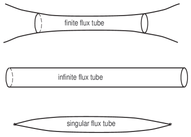
Figure 1: The gravitational flux tubes with the different relation between electric $q$ and magnetic $Q$ charges.

Most important for us here is the case with $\delta=1-\frac{Q}{q}\ll 1$. From Eq. (2.14) we have $q=2a_{0}\sin(\pi/4+\delta)\approx a_{0}\sqrt{2}(1+\delta)$ and $Q\approx a_{0}\sqrt{2}(1-\delta)$.

3 Infinite flux tube solution

In this section we would like to present in details the infinite flux tube solution with $E=H$ as this metric is very good approximation for central part of solutions with $\delta\ll 1$. The metric is the solution of Eq’s (2.6)-(2.9)

$$ds^{2} = \cosh\left(\frac{r\sqrt{2}}{q}\right)dt^{2}-\left[d\chi+\sqrt{2}\sinh\left(\frac{r\sqrt{2}}{q}\right)dt+Q\cos\theta d\varphi\right]^{2}-$$ (3.2)

$$dr^{2}-\frac{q^{2}}{2}\left(d\theta^{2}+\sin^{2}\theta d\varphi^{2}\right)=$$

$$\left[1-\sinh^{2}\left(\frac{r\sqrt{2}}{q}\right)\right]dt^{2}-Q^{2}\left(\frac{d\chi}{Q}+\cos\theta d\varphi\right)^{2}-\frac{q^{2}}{2}\left(d\theta^{2}+\sin^{2}\theta d\varphi^{2}\right)-$$

$$dr^{2}-2\sqrt{2}\sinh\left(\frac{r\sqrt{2}}{q}\right)\left(d\chi+Q\cos\theta d\varphi\right)dt.$$

From the last form (3.2) of the metric we see that the terms

$$dl^{2}=Q^{2}\left(\frac{d\chi}{Q}+\cos\theta d\varphi\right)^{2}+\frac{q^{2}}{2}\left(d\theta^{2}+\sin^{2}\theta d\varphi^{2}\right)$$ (3.3)

are like to the standard metric

$$dl^{2}=\left(\frac{d\chi}{Q}+\cos\theta d\varphi\right)^{2}+\left(d\theta^{2}+\sin^{2}\theta d\varphi^{2}\right)$$ (3.4)

on the $S^{3}-$sphere where $S^{3}-$sphere is presented as the Hopf bundle $S^{3}\rightarrow S^{2}$ with the $S^{1}-$sphere as the fibre. The first term of Eq. (3.2) tells us that the time $t$ is not everywhere the true time coordinate as for $r>r_{1}$ the metric component $G_{tt}=1-\sinh^{2}\left(\frac{r\sqrt{2}}{q}\right)<0$.

The metric (3.2) is very interesting in the following context. It has the form of dynamical splitting off the $5^{th}-$dimension as $G_{55}=1$. The origin of such splitting off is the presence of off-diagonal components of 5D metric $G_{5t}$ and $G_{5}\varphi$ which are electromagnetic potential components. From the physical point of view it is the consequence of the presence of electric and magnetic fields with very special constraint: $E=H$. Mathematically it is an exceptional solution of (2.6)-(2.9) equations.

Another interesting question from the infinite flux tube metric (3.2) is the question about clock reading. The metric (3.2) shows that clock reading is

$$d\tau_{5}=dt\sqrt{1-\sinh^{2}\left(\frac{r\sqrt{2}}{q}\right)}=dt\sqrt{G_{00}-A_{0}^{2}}.$$ (3.5)

Let us compare this 5D infinite flux tube solution with the Levi-Civita - Robertson - Bertotti flux tubes solutions [2]. It is an infinite flux tube filled with parallel electric $F_{01}$ and and magnetic $F_{23}$ fields

$$ds^{2} = a^{2}\left(\cosh^{2}\zeta dt^{2}-d\zeta^{2}-d\theta^{2}-\sin^{2}\theta d\varphi^{2}\right),$$ (3.6)

$$F_{01} = \rho^{1/2}\cos\alpha,\;\;\;\;\;\;\;F_{23}=\rho^{1/2}\sin\alpha,$$ (3.7)

where

$$G^{1/2}a\rho^{1/2}=1.$$ (3.8)

$\alpha$ is an arbitrary constant angle; $a$ and $\rho$ are constants defined by Eq. (3.8); $a$ determines the cross section of the tube and $\rho$ the magnitude of the electric and magnetic fields; $G$ is Newton’s constant ($c=1$, the speed of light); $F_{\mu\nu}$ is the electromagnetic field tensor. For $\cos\alpha=1$ ($\sin\alpha=1$) one has a purely electric (or magnetic) field. This 4D solution is the analog of the 5D flux tube solution with only one difference: electric and magnatic fields can be different. Clock reading for 4D solution is

$$d\tau_{4}=\cosh\left(\frac{r\sqrt{2}}{q}\right)dt.$$ (3.9)

Physically this remark allows us to determine experimentally: is the dimension of our spacetime four or more.

4 Superlong solutions

Now we would like to consider the case with $\delta=1-Q/q\ll 1$. In this section we will show that every such object with cross section $\approx l^{2}_{Pl}$ can be considered as a string-like object.

At first we will investigate solutions of Eq’s (2.6)-(2.9) for different $\delta$’s. The numerical investigations of these equations set show us that the solution is very insensitive to $\delta\ll 1$. In order to avoid this problem we introduce the following new functions

$$\Delta(x) = \frac{f(x)}{\cosh^{2}(x)},$$ (4.1)

$$\psi(x) = \phi(x)+\ln\cosh(x)$$ (4.2)

where $x=r/a(0)^{1/2}$ is a dimensionless radius. In the case $f(x)=1$ and $\phi(x)=0$ we have the above-mentioned infinite flux tube. Thus we have the following equations for the functions (4.1) (4.2)

$$f^{\prime\prime}-4f^{\prime}\tanh(x)-2f\left(1-3\tanh^{2}(x)\right)-\frac{\left(f^{\prime}-2f\tanh(x)\right)^{2}}{f}+$$

$$\frac{a^{\prime}}{a}\left(f^{\prime}-2f\tanh(x)\right)+\left(f^{\prime}-2f\tanh(x)\right)\left(\phi^{\prime}+\tanh(x)\right)+\frac{q^{2}}{a^{2}f}e^{-4\phi}=0,$$ (4.3)

$$a^{\prime\prime}-2+a^{\prime}\left(\phi^{\prime}+\tanh(x)\right)+\frac{Q^{2}f}{a}e^{2\phi}=0,$$ (4.4)

$$\phi^{\prime\prime}+\frac{1}{\cosh^{2}(x)}+\left(\phi^{\prime}+\tanh(x)\right)^{2}+\frac{a^{\prime}}{a}\left(\phi^{\prime}+\tanh(x)\right)-\frac{Q^{2}f}{2a^{2}}e^{2\phi}=0$$ . (4.5)

The corresponding solutions of these equations with the different $\delta$ are presented on Fig’s (4)-(4).

Figure 2: The functions $a(x)$ in accordance with the different relation between electric and magnetic charges. The curves 1,2,3,4 correspond to the following magnitudes of $\delta=10^{-3},10^{-6},10^{-10},10^{-13}$.

Figure 3: The functions $f(x)$ in accordance with the different relation between electric and magnetic charges. The curves 1,2,3,4 correspond to the following magnitudes of $\delta=10^{-3},10^{-6},10^{-10},10^{-13}$.

Figure 4: The functions $\phi(x)$ in accordance with the different relation between electric and magnetic charges. The curves 1,2,3,4 correspond to the following magnitudes of $\delta=10^{-3},10^{-6},10^{-10},10^{-13}$.

We see that (at least in the investigated area of $\delta$) at the point $r=\pm r_{H}$ the function $a(r_{H})\approx 2a_{0}$ (here $r_{H}$ is the point where $\Delta(r_{H})=0$). The most interesting aspect is that $a(r_{H})$ does not grow as $r\rightarrow\pm r_{H}$ and consequently the flux tube with $\delta\ll 1$ (in the region $|r|\leq r_{H}$) can be considered as a string-like object attached to two Universes.

All this shows us that the conditions which are necessary for the consideration of the presented solution as a string-like object definitely are satysfied in the region $|r|\leq r_{H}$ but outside of this region the cross section will increase and spacetime is asymptotically flat. It is easy to see for the special case $Q=0$ [1]. In this case there is the exact solution

$$a = r^{2}_{0}+r^{2},$$ (4.6)

$$\Delta = \frac{q}{2r_{0}q}\frac{r^{2}_{0}-r^{2}}{r^{2}_{0}+r^{2}},$$ (4.7)

$$\psi = 0,$$ (4.8)

$$\omega = \frac{4r_{0}}{q}\frac{r}{r^{2}_{0}-r^{2}}$$ (4.9)

and we see that $a\approx r^{2}$ (at $a\rightarrow\infty$) and $g_{tt}\approx-1+\mathcal{O}(1/r^{2})$, the same is for the others cases with $Q<q$.

The thickness of the gravitational flux tube can be arbitrary small and we choose its in the Planck region. In this case near to the attachment point of the tube to an external Universe the quantum wormholes of a spacetime foam will appear between this object and the Universe. This is like a delta of the river flowing into the sea, see Fig. 5. This remark allows us to call the super-long and thin gravitational flux tube as the $\Delta-$string.

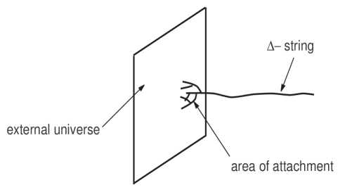
Figure 5: The attachment point of $\Delta-$string to an external Universe.

5 The metric close to $r=\pm r_{H}$

Now we would like to show that the $\Delta-$string solution is nonsingular at the points $\pm r_{H}$ where $\Delta(\pm r_{H})=0$. For this we investigate the solution behaviour near to the point $|r|\approx r_{H}$ where

$$a(r) = a_{0}+a_{1}\left(r-r_{H}\right)+a_{2}\left(r-r_{H}\right)^{2}+\cdots,$$ (5.1)

$$\psi(r) = \psi_{H}+\psi_{1}\left(r-r_{H}\right)+\psi_{2}\left(r-r_{H}\right)^{2}+\cdots,$$ (5.2)

$$\Delta(r) = \Delta_{1}\left(r-r_{H}\right)+\Delta_{2}\left(r-r_{H}\right)^{2}+\cdots.$$ (5.3)

The substitution in Eq’s (2.6)-(2.9) gives us the following solution

$$\Delta_{1} = \pm qe^{-2\psi_{H}},\quad(+)\quad\text{for}\quad r\rightarrow-r_{H}\quad\text{and}\quad(-)\quad\text{for}\quad r\rightarrow+r_{H},$$ (5.4)

$$\psi_{2} = -\psi_{1}\frac{a_{1}+a_{0}\psi_{1}}{2a_{0}},$$ (5.5)

$$\Delta_{2} = \frac{-3a_{0}\psi_{1}+a_{1}}{2a_{0}},$$ (5.6)

$$a_{2} = \frac{2-a_{1}\psi_{1}}{2}.$$ (5.7)

In this case equation (2.10) has the following behaviour near to the points $r=\pm r_{H}$

$$\omega^{\prime}(r)=\frac{a_{0}e^{\psi_{H}}}{q}\frac{1}{\left(r-r_{H}\right)^{2}}+\omega_{1}+\mathcal{O}\left(r-r_{H}\right)$$ (5.8)

where $\omega_{1}$ is some constant depending on $a_{0,1},\psi_{1,2},\Delta_{1,2}$. It leads to the following $\omega(r)$ behaviour

$$\omega(r)=-\frac{a_{0}e^{\psi_{H}}}{q}\frac{1}{\left(r-r_{H}\right)}+\omega_{0}+\mathcal{O}\left(r-r_{H}\right)$$ (5.9)

where $\omega_{0}$ is some integration constant. The $G_{tt}$ metric component is

$$G_{tt}=\frac{a(r)}{\Delta(r)}-\frac{\Delta(r)e^{2\psi(r)}}{a(r)}\omega^{2}(r)=-e^{2\psi_{H}}\frac{2qe^{-\psi_{H}}\omega_{0}-a_{1}-a_{0}\psi_{1}}{q}+\mathcal{O}\left(r-r_{H}\right).$$ (5.10)

Then the metric (2.3) has the following approximate behaviour near to $r=\pm r_{H}$ points

$$\begin{split}ds^{2}=&\left[g_{H}+\mathcal{O}\left(r-r_{H}\right)\right]dt^{2}-\mathcal{O}\left(r-r_{H}\right)\left(d\chi+Q\cos\theta d\varphi\right)^{2}-\\ &\left[e^{\psi_{H}}+\mathcal{O}\left(r-r_{H}\right)\right]dt\left(d\chi+Q\cos\theta d\varphi\right)-dr^{2}-\\ &\left[a(r_{H})+\mathcal{O}\left(r-r_{H}\right]\right)\left(d\theta^{2}+\sin^{2}\theta d\varphi^{2}\right)\approx\\ &e^{\psi_{H}}dt\left(d\chi+Q\cos\theta d\varphi\right)-dr^{2}-a(r_{H})\left(d\theta^{2}+\sin^{2}\theta d\varphi^{2}\right)\end{split}$$ (5.11)

where $g_{H}=-e^{2\psi_{H}}\left(2qe^{-\psi_{H}}\omega_{0}-a_{1}-a_{0}\psi_{1}\right)/q$. It means that at the points $r=\pm r_{H}$ the metric (2.3) is nonsingular.

6 Approximate analytical solution close to pure electric solution with $Q=0$

In this section we would like to investigate analytically the metric close to exact solution with $Q=0$.

$$a(r) = a_{0}(r)+\delta a(r),$$ (6.1)

$$\Delta(r) = \Delta_{0}(r)+\delta\Delta(r),$$ (6.2)

$$\psi(r) = \psi_{0}(r)+\delta\psi(r)$$ (6.3)

and $Q$ is small parameter $Q^{2}/a(0)\ll 1$.

$$a_{0}(r) = r^{2}+r_{0}^{2},$$ (6.4)

$$\Delta_{0}(r) = r_{0}^{2}-r^{2},$$ (6.5)

$$\psi_{0}(r) = 0$$ (6.6)

the functions $a_{0}(r),\Delta_{0}(r)$ and $\psi_{0}(r)$ are the solutions of Einstein equations with $Q=0$. The variation of equations (2.6)-(2.9) with respect to small perturbations $\delta a(r),\delta\Delta(r)$ and $\delta\psi(r)$ give us the following equations set

$$\delta\psi+\frac{a^{\prime}_{0}}{a_{0}}\delta\psi^{\prime}-\frac{Q^{2}\Delta_{0}}{2a_{0}^{3}} = 0,$$ (6.7)

$$\delta a^{\prime\prime}+a^{\prime}_{0}\delta\psi^{\prime}+\frac{Q^{2}\Delta_{0}}{a_{0}^{2}} = 0,$$ (6.8)

$$\delta\Delta^{\prime\prime}-\frac{a^{\prime}_{0}}{a_{0}}\delta\Delta^{\prime}-\frac{\Delta^{\prime}_{0}\delta a^{\prime}}{a_{0}}+\frac{\Delta^{\prime}_{0}a^{\prime}_{0}}{a_{0}^{2}}\delta a+3\Delta^{\prime}_{0}\delta\psi^{\prime}+2\frac{\delta\Delta}{a_{0}}-2\frac{\Delta_{0}}{a_{0}^{2}}\delta a = 0.$$ (6.9)

The solution of this system is

$$\delta\psi(r) = -\frac{1}{4}\frac{Q^{2}}{r^{2}+r_{0}^{2}},$$ (6.10)

$$\delta a(r) = -\frac{Q^{2}}{2}\frac{r}{r_{0}}\arctan\left(\frac{r}{r_{0}}\right)+\frac{Q^{2}}{4},$$ (6.11)

$$\delta\Delta(r) = \frac{Q^{2}}{2}\left[\frac{r}{r_{0}}\arctan\left(\frac{r}{r_{0}}\right)-\frac{r^{2}-r_{0}^{2}}{r^{2}+r_{0}^{2}}+\frac{1}{2}\right].$$ (6.12)

Substituting into equation (11.11) gives us

$$a(r)+\Delta(r)e^{2\psi(r)}=2r_{0}^{2}+\frac{Q^{2}}{2}$$ (6.13)

but

$$a(r)\approx r_{0}^{2}+r^{2}-\frac{Q^{2}}{2}\frac{r}{r_{0}}\arctan\left(\frac{r}{r_{0}}\right)+\frac{Q^{2}}{4}$$ (6.14)

and

$$a(0)\approx r_{0}^{2}+\frac{Q^{2}}{4}$$ (6.15)

therefore

$$a(r)+\Delta(r)e^{2\psi(r)}=2a(0)$$ (6.16)

with an accuracy of $Q^{2}$.

7 Solutions expanded into a series

In this section we will derive the solution of Eq’s set (2.6)-(2.9) by expansion in terms of $r$. Using the MAPLE package we have obtained the solution with accuracy of $r^{12}$

$$\psi(x) = \frac{1}{4}{\tilde{Q}}^{2}{x}^{2}+\left({\frac{5}{48}}{\tilde{Q}}^{4}-\frac{1}{4}{\tilde{Q}}^{2}\right){x}^{4}+\left(-{\frac{7}{30}}{\tilde{Q}}^{4}+{\frac{41}{720}}{\tilde{Q}}^{6}+\frac{1}{4}{\tilde{Q}}^{2}\right){x}^{6}$$ (7.1)

$$+\left(-\frac{1}{4}{\tilde{Q}}^{2}+{\frac{213}{560}}{\tilde{Q}}^{4}-{\frac{111}{560}}{\tilde{Q}}^{6}+{\frac{281}{8064}}{\tilde{Q}}^{8}\right){x}^{8}+$$

$$\left(-{\frac{341}{630}}{\tilde{Q}}^{4}+{\frac{3749}{8400}}{\tilde{Q}}^{6}-{\frac{1553}{9450}}{\tilde{Q}}^{8}+{\frac{5147}{226800}}{\tilde{Q}}^{10}+\frac{1}{4}{\tilde{Q}}^{2}\right){x}^{10}+O\left({x}^{12}\right),$$

$$\Delta(x) = 1-{x}^{2}+\left(\frac{5}{6}{\tilde{Q}}^{2}-\frac{1}{4}{\tilde{Q}}^{4}\right){x}^{4}+\left(-{\frac{9}{10}}{\tilde{Q}}^{2}+{\frac{47}{90}}{\tilde{Q}}^{4}-\frac{1}{12}{\tilde{Q}}^{6}\right){x}^{6}+$$ (7.2)

$$\left(-\frac{6}{7}{\tilde{Q}}^{4}+{\frac{373}{1260}}{\tilde{Q}}^{6}-{\frac{3}{80}}{\tilde{Q}}^{8}+{\frac{13}{14}}{\tilde{Q}}^{2}\right){x}^{8}+$$

$$\left({\frac{218}{175}}{\tilde{Q}}^{4}-{\frac{2893}{4200}}{\tilde{Q}}^{6}+{\frac{5219}{28350}}{\tilde{Q}}^{8}-{\frac{17}{18}}{\tilde{Q}}^{2}-{\frac{37}{1890}}{\tilde{Q}}^{10}\right){x}^{10}+O\left({x}^{12}\right),$$

$$a(x) = 1+\left(1-\frac{1}{2}{\tilde{Q}}^{2}\right)\left[{x}^{2}+\frac{1}{6}{\tilde{Q}}^{2}{x}^{4}+\left(-\frac{1}{10}{\tilde{Q}}^{2}+{\frac{11}{180}}{\tilde{Q}}^{4}\right){x}^{6}+\right.$$ (7.3)

$$\left.\left(-{\frac{13}{140}}{\tilde{Q}}^{4}+{\frac{73}{2520}}{\tilde{Q}}^{6}+\frac{1}{14}{\tilde{Q}}^{2}\right){x}^{8}+\right.$$

$$\left.\left({\frac{239}{2100}}{\tilde{Q}}^{4}+{\frac{887}{56700}}{\tilde{Q}}^{8}-\frac{1}{18}{\tilde{Q}}^{2}-{\frac{13}{175}}{\tilde{Q}}^{6}\right){x}^{10}\right]+O\left({x}^{12}\right)$$

here we have introduced the following dimensionless parameter : $\tilde{Q}=Q/\sqrt{a(0)}$. The substitution in Eq. (11.11) shows that it is valid.

One of the most important question here is : how long is the $\Delta-$string ? Let us determine the length of the $\Delta-$string as $2r_{H}$ where $r_{H}$ is the place where $ds^{2}(\pm r_{H})=0$ (at these points $\Delta(\pm r_{H})=0$). This is very complicated problem because we have not the analytical solution and the numerical calculations indicate that $r_{H}$ depends very weakly from $\delta=(1-Q/q)$ parameter : the big magnitude of this parameter leads to the relative small magnitude of $r_{H}$. The expansion (7.3) allows us to assume that

$$a(r)=a(0)+a_{1}(r,Q)\,\delta_{1}$$ (7.4)

here $\delta_{1}=1-Q^{2}/Q_{0}^{2}$; $Q_{0}^{2}=2a(0)$. If $Q\approx Q_{0}=\sqrt{2a(0)}$ then

$$a(r)\approx a(0)+a_{1}(r,Q_{0})\,\delta_{1}.$$ (7.5)

Using the MAPLE package we have obtained $a_{1}(r)$ with accuracy of $r^{20}$

$$\begin{split}a_{1}(x)={x}^{2}+\frac{1}{3}{x}^{4}+{\frac{2}{45}}{x}^{6}+{\frac{1}{315}}{x}^{8}+{\frac{2}{14175}}{x}^{10}+\\ {\frac{2}{467775}}{x}^{12}+{\frac{4}{42567525}}{x}^{14}+{\frac{1}{638512875}}{x}^{16}+{\frac{2}{97692469875}}{x}^{18}+O\left({x}^{20}\right).\end{split}$$ (7.6)

It is easy to see that this series coincides with $\cosh^{2}(x)-1$. Therefore we can assume that in the first rough approximation

$$a(r)\approx a(0)\left\{1+\left(1-\frac{Q^{2}}{Q_{0}^{2}}\right)\left[\cosh^{2}\left(\frac{r}{\sqrt{a(0)}}\right)-1\right]\right\}.$$ (7.7)

It allows us to estimate the length $L=2r_{H}$ of the $\Delta-$string from equation (11.11) as

$$a(r_{H})=a(0)\left\{1+\delta_{1}\left[\cosh^{2}\left(\frac{r_{H}}{\sqrt{a(0)}}\right)-1\right]\right\}=2a(0).$$ (7.8)

For $r_{H}\gg\sqrt{a(0)}$ we have

$$L\approx\sqrt{a(0)}\ln\frac{1}{\delta_{1}}.$$ (7.9)

One can compare this result with the numerical calculations : $\delta_{1}=10^{-10}$, $r_{H}/\sqrt{a(0)}\approx 15$, $\frac{1}{2}\ln 1/\delta_{1}\approx 15$; $\delta_{1}=10^{-9}$, $r_{H}/\sqrt{a(0)}\approx 11$, $\frac{1}{2}\ln 1/\delta_{1}\approx 10$; $\delta_{1}=10^{-8}$, $r_{H}/\sqrt{a(0)}\approx 10$, $\frac{1}{2}\ln 1/\delta_{1}\approx 9$. We see that $r_{H}/\sqrt{a(0)}$ and $\ln 1/\delta_{1}$ have the same order. This evaluation should be checked up (in future investigations) more carefully as the convergence radius of our expansion (7.1)-(7.3) is unknown.

8 The qualitative model of the $\Delta-$string

The numerical calculations presented on Fig’s (4)-(4) show that the $\Delta-$string approximately can be presented as a finite tube with the constant cross section and a big length joint at the ends with two short tubes which have variable cross section, see Fig. (6).

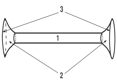
Figure 6: The qualitative model of the $\Delta-$string. 1 is the part of the infinite flux tube solution. 2 are two cones which are pure electric solutions, 3 are two hypersurfaces where $ds^{2}=0$.

For the model of the central tube we take the part of the infinite flux tube solution with $Q=q=Q_{0}$ [1]

$$a_{\infty}=\frac{Q_{0}^{2}}{2}=const,$$ (8.1)

$$e^{\psi}=\frac{a_{\infty}}{\Delta}=\cosh\frac{r}{\sqrt{a_{\infty}}},$$ (8.2)

$$\omega=\sqrt{2}\sinh\frac{r}{\sqrt{a_{\infty}}}$$ (8.3)

here we have parallel electric $E$ and magnetic $H$ fields with equal electric $q$ and magnetic $Q$ charges.

For a model of two peripheral ends (cones) we take the solution with $Q=0$ (equations (6.4)-(6.6)). Here we have only the electric field $E$. At the ends of the $\Delta-$string ($r=\pm r_{H}$) the function $\Delta(\pm r_{H})=0$ and the term $Q^{2}\Delta e^{2\psi}/a^{3}$ in equations (2.6)-(2.9) is zero that allows us to set this term as zero at the peripheral cones.

We have to join the components of metric on the $r=r_{1}=r_{H}-\sqrt{a(0)}$ (here $a(0)=a_{\infty}$).

$$\cosh^{2}\left(\frac{r_{1}}{\sqrt{a(0)}}\right)=\frac{\tilde{a}(r_{1})}{\tilde{\Delta}(r_{1})}=\tilde{g}_{tt}(r_{1})=\tilde{\tilde{g}}_{tt}(r_{1})=\frac{\tilde{\tilde{a}}(r_{1})}{\tilde{\tilde{\Delta}}(r_{1})}$$ (8.4)

here $\tilde{}$ and $\tilde{\tilde{}}$ mean that the corresponding quantities are the metric components for $Q=Q_{0}$ and $Q=0$ solutions respectively. According to equations (6.4)-(6.6)

$$\tilde{\tilde{a}}(r) = a(0)+\left(r-r_{1}\right)^{2},$$ (8.5)

$$\tilde{\tilde{\Delta}}(r) = \alpha\left[a(0)-\left(r-r_{1}\right)^{2}\right]$$ (8.6)

$$\tilde{\tilde{a}}(r_{1}) = \tilde{a}(r_{1})=a(0)$$ (8.7)

here $r_{0}^{2}$ from equation (6.4)-(6.6) is replaced with $\tilde{\tilde{a}}(0)$ and some coefficient $\alpha$ is introduced as Eq’s (2.6)-(2.9) with $Q=0$ have the terms like $\Delta^{\prime\prime}/\Delta$ and $\Delta^{\prime}/\Delta$ only. It gives us

$$\alpha=\frac{1}{\cosh^{2}\left(\frac{r_{1}}{\sqrt{a(0)}}\right)}\approx 4e^{\frac{-2r_{1}}{\sqrt{a(0)}}}$$ (8.8)

since for the long $\Delta-$string $r_{1}/\sqrt{a(0)}\gg 1$. The next joining is for

$$1=\frac{\tilde{\Delta}(r_{1})e^{2\tilde{\psi}(r_{1})}}{\tilde{a}(r_{1})}=\tilde{g}_{55}(r_{1})=\tilde{\tilde{g}}_{55}(r_{1})=\frac{\tilde{\tilde{\Delta}}(r_{1})e^{2\tilde{\tilde{\psi}}(r_{1})}}{\tilde{\tilde{a}}(r_{1})}$$ (8.9)

here the constant term $2\tilde{\tilde{\psi}}_{1}$ is added to solution (6.6) $2\psi_{0}=0$ since again equations (2.6)-(2.9) have $\psi^{\prime\prime}$ and $\psi^{\prime}$ terms only. Consequently

$$e^{2\tilde{\tilde{\psi}}_{1}}=\frac{1}{\alpha}\approx\frac{e^{2r_{1}/\sqrt{a(0)}}}{4}\quad\text{or}\quad\psi_{1}\approx\frac{r_{1}}{\sqrt{a(0)}}-\ln 4.$$ (8.10)

The last component of the metric is

$$a(0)=a_{\infty}=\tilde{g}_{\theta\theta}(r_{1})=\tilde{\tilde{g}}_{\theta\theta}(r_{1})=\tilde{\tilde{a}}(r_{1}).$$ (8.11)

For the electric field we have

$$\tilde{E}(r_{1}) = \frac{qe^{\tilde{\psi}(r_{1})}}{a(0)}=\frac{q}{a(0)}\cosh\left(\frac{r_{1}}{\sqrt{a(0)}}\right)=\frac{q}{a(0)}\frac{1}{\sqrt{\alpha}}$$ (8.12)

$$\tilde{\tilde{E}}(r_{1}) = q\frac{\tilde{\tilde{a}}(r_{1})}{\tilde{\tilde{\Delta}}^{2}(r_{1})}e^{-3\tilde{\tilde{\psi}}(r_{1})}=\frac{q}{a(0)}\frac{1}{\sqrt{\alpha}}$$ (8.13)

and consequently

$$\tilde{E}(r_{1})=\tilde{\tilde{E}}(r_{1}).$$ (8.14)

Thus our final result for this section is that at the first rough approximation the $\Delta-$string looks like to a tube with constant cross section and two cones attached to its ends.

In this section we have considered an approximate model of the $\Delta-$string. The purpose of this model is to show visually how is the form of the $\Delta-$string since it is not clear from the approximate calculations. From this point of view we do not demand the continuity of the metric derivatives as this model helps us only to understand what is it the $\Delta-$string on a qualitative level. Nevertheless we should not forget that the cross section of the long tube and all sizes of two peripheral cones are in Planck region and consequently quantum fluctuations can make unessential requirements to a continuity of classical degrees of freedom.

9 $\Delta-$string as a model of electric charge

In this section we would like to present a model of attachment of the $\Delta-$string to a spacetime.

May be the most important question for the $\Delta-$string is : what will see an external observer living in the Universe to which the $\Delta-$string is attached. Whether he will see a dyon with electric and magnetic fields or an electric charge ? This question is not very simple as it is not very clear what is it the electric and magnetic fields on the $\Delta-$string. Are they the tensor $F_{\mu\nu}$ and fields $E_{i}$ and $H_{i}$

$$F_{\mu\nu} = \partial_{\mu}A_{\nu}-\partial_{\nu}A_{\mu},\quad\mu,\nu=0,1,2,3,$$ (9.1)

$$E_{i} = F_{0i},\quad i,j,k=1,2,3,$$ (9.2)

$$H_{i} = e_{ijk}F^{jk}$$ (9.3)

or something another that is like to an electric displacement $D_{i}=\varepsilon E_{i}$ and $H_{i}=\mu B_{i}$ ? The answer on this question depends on the way how we will continue the solution behind the hypersurface $r=\pm r_{H}$ (where $ds^{2}=0$). We have two possibilities : the first way is the simple continuation our solution to $|r|>r_{H}$, the second way is a string approach - attachment the $\Delta-$string to a spacetime. In the first case $\Delta(r)>0$ by $|r|<r_{H}$ and $\Delta(r)<0$ by $|r|>r_{H}$ it means that by $|r|>r_{H}$ the time and 5th coordinate $\chi$ becomes respectively space-like and time-like dimensions. It is not so good for us. The second approach is like to a string attached to a D-brane. We believe that physically the second way is more interesting.

Let us consider Maxwell equations in the 5D Kaluza-Klein theory

$$R_{5\mu}=\frac{1}{\sqrt{-g}}\partial_{\nu}\left(\sqrt{-g}g_{55}F^{\mu\nu}\right)=0$$ (9.4)

here $g=\det{g_{AB}=a^{4}\sin^{2}\theta e^{2\psi}}$. These 5D Maxwell equations are similar to Maxwell equations in the continuous medium where the factor $\sqrt{-g}g_{55}$ is like to a permittivity for $R_{50}$ equation and a permeability for $R_{5i}$ equations. It allows us offer the following conditions for matching the electric and magnetic fields at the attachment point of $\Delta-$ string to the spacetime

$$\sqrt{-g_{\Delta}}{g_{\Delta}}_{55}F^{0i}_{\Delta} = \sqrt{-g}F^{0i}$$ (9.5)

$$\sqrt{-g_{\Delta}}{g_{\Delta}}_{55}F^{ij}_{\Delta} = \sqrt{-g}F^{ij}$$ (9.6)

here the subscript $\Delta$ means that this quantity is given on the $\Delta-$string and on l.h.s there are the quantities belonging to the $\Delta-$string and on the r.h.s. the corresponding quantities belong to the spacetime to which we want to attach the $\Delta-$string. As an example one can join the $\Delta-$string to the Reissner-Nordström solution with the metric

$$ds^{2}=e^{2\nu}dt^{2}-e^{-2\nu}dr^{2}-r^{2}\left(d\theta^{2}+\sin^{2}\theta d\varphi^{2}\right).$$ (9.7)

Then on the $\Delta-$string

$$\sqrt{-g_{\Delta}}{g_{\Delta}}_{55}F^{tr}_{\Delta}=-\frac{\Delta^{2}e^{3\psi}}{a}\omega^{\prime}=-a\frac{q}{a}$$ (9.8)

For the Reissner-Nordström solution

$$\sqrt{-g}F^{tr}=-r^{2}E_{r(RN)}.$$ (9.9)

Therefore after joining on the event horizon $r=r_{H}$ ($a=a_{H}$) we have

$$E_{r(RN)}=\frac{q}{a_{H}}$$ (9.10)

here we took into account that $a_{H}=r^{2}_{H}$.

For equation (9.6) we have

$$\sqrt{-g_{\Delta}}{g_{\Delta}}_{55}F^{\theta\varphi}_{\Delta}=\frac{Q\Delta e^{3\psi}}{a^{2}}.$$ (9.11)

On the surface of joining $\Delta(r_{H})=0$ consequently we have very unexpected result : the continuation of $F^{\theta\varphi}$ (and magnetic field $H_{r}$) from the $\Delta-$string to the spacetime (D-brane) gives us zero magnetic field $H_{r}$.

Finally our result for this section is that the $\Delta-$string can be attached to a spacetime by such a way that it looks like to an electric charge but not magnetic one. Such approach to the geometrical interpretation of electric charges suddenly explain why we do not observe magnetic charges in the world.

10 Waves on the $\Delta-$string

In this section we will consider small perturbations of 5D metric. Generally speaking they are 5D gravitational waves on the gravitational flux tube (or on the string language - vibrations of $\Delta-$string). In the general case 5D metric is

$$ds^{2}=g_{\mu\nu}dx^{\mu}dx^{\nu}-\phi^{2}\left(d\chi+A_{\mu}dx^{\mu}\right)^{2}$$ (10.1)

here $g_{\mu\nu}$ is the 4D metric; $\mu,\nu=0,1,2,3$; $A_{\mu}$ is the electromagnetic potential; $\phi$ is the scalar field. The corresponding 5D Kaluza-Klein’s equations are (for the reference see, for example, [3])

$$R_{\mu\nu}-\frac{1}{2}g_{\mu\nu}R = -\frac{\phi^{2}}{2}T_{\mu\nu}-\frac{1}{\phi}\left[\nabla_{\mu}\left(\partial_{\nu}\phi\right)-g_{\mu\nu}\Box\phi\right],$$ (10.2)

$$\nabla_{\nu}F^{\mu\nu} = -3\frac{\partial_{\nu}\phi}{\phi}F^{\mu\nu},$$ (10.3)

$$\Box\phi = -\frac{\phi^{3}}{4}F^{\alpha\beta}F_{\alpha\beta}$$ (10.4)

where $R_{\mu\nu}$ is the 4D Ricci tensor; $F_{\mu\nu}=\partial_{\mu}A_{\nu}-\partial_{\nu}A_{\mu}$ is the 4D Maxwell tensor and $T_{\mu\nu}$ is the energy-momentum tensor for the electromagnetic field.

We will consider only $\delta A_{\mu}$ perturbations, $\delta g_{\mu\nu}$ and $\delta\phi$ degrees of freedom are frozen. For this approximation we have equation

$$\nabla_{\nu}\delta F^{\mu\nu}=0.$$ (10.5)

We introduce only one small perturbation in the electromagnetic potential

$$\delta A_{\theta}=f(t,r)$$ (10.6)

since for the background metric $\phi=const$. Generally speaking $A_{\theta}$-component should have some dependence on the $\theta$-angle. But the cross section of the $\Delta-$string is in Planck region and consequently the points with different $\theta$ and $\varphi$ ($r$ = const) physically are not distinguishable. Therefore all physical quantities on the $\Delta-$string should be averaged over polar angles $\theta$ and $\varphi$. It means that the $\delta A_{\theta}$ in Eq. (13.10) is averaged quantity.

After such) remark we have the following wave equation for the function $f(t,r)$

$$\partial_{tt}f(t,x)-\cosh x\partial_{x}\biggl{(}\cosh x\partial_{x}f(t,x)\biggl{)}=0$$ (10.7)

here we have introduced the dimensionless variables $t/\sqrt{a(0)}\rightarrow t$ and $r/\sqrt{a(0)}\rightarrow x$. The solution is

$$f(t,x)=f_{0}F\left(t-2\arctan e^{x}\right)+f_{1}F\left(t+2\arctan e^{x}\right)$$ (10.8)

here $f_{0,1}$ are some constants and $F$ and $H$ are arbitrary functions. This solution has more suitable form if we introduce new coordinate $y=2\arctan e^{x}$. Then

$$f(t,y)=f_{0}F(t-y)+f_{1}H(t+y).$$ (10.9)

The metric is

$$ds^{2}=\frac{a_{0}}{\sin^{2}y}dt^{2}-\frac{dy^{2}}{\sin^{2}y}-a_{0}\left(d\theta^{2}+\sin^{2}\theta d\varphi^{2}\right)-\left(d\chi+\omega dt+Q\cos\theta d\varphi\right)^{2}.$$ (10.10)

Thus the simplest solution is electromagnetic waves moving in both directions along the $\Delta-$string.

11 The comparison with string theory

Now we want to compare this situation with the situation in string theory. How is the difference between the result presented in Section 10 (Eq’s (10.7), (10.8)) and the string oscillation in the ordinary string theory ? The action for bosonic string is

$$S=-\frac{T}{2}\int d^{2}\sigma\sqrt{h}h^{ab}\partial_{a}\mathcal{X}^{\mu}\partial_{b}\mathcal{X}_{\mu}$$ (11.1)

here $\sigma^{a}=\{\sigma,\tau\}$ is the coordinates on the world sheet of string; $\mathcal{X}^{\mu}$ are the string coordinates in the ambient spacetime; $h_{ab}$ is the metric on the world sheet. The variation with respect to $\mathcal{X}^{\mu}$ give us the usual 2D wave equation

$$\Box\mathcal{X}^{\mu}\equiv\left(\frac{\partial^{2}}{\partial\sigma^{2}}-\frac{\partial^{2}}{\partial\tau^{2}}\right)\mathcal{X}^{\mu}=0$$ (11.2)

which is similar to Eq. (10.7). The difference is that the variation of the action (11.1) with respect to the metric $h^{ab}$ gives us some constraints equations in string theory

$$T_{ab}=\partial_{a}\mathcal{X}^{\mu}\partial_{b}\mathcal{X}_{\mu}-\frac{1}{2}h_{ab}h^{cd}\partial_{c}\mathcal{X}^{\mu}\partial_{d}\mathcal{X}_{\mu}=0$$ (11.3)

but for $\Delta-$string analogous variation gives the dynamical equation for 2D metric $h_{ab}$.

The more detailed description is the following. The topology of 5D Kaluza-Klein spacetime is $M^{2}\times S^{2}\times S^{1}$ where $M^{2}$ is the 2D space-time spanned on the time and longitudinal coordinate $r$; $S^{2}$ is the cross section of the flux tube solution and it is spanned on the ordinary spherical coordinates $\theta$ and $\varphi$; $S^{1}=U(1)$ is the Abelian gauge group which in this consideration is the 5th dimension. The initial 5D action for $\Delta-$string is

$$S=\int\sqrt{-\stackrel{{\scriptstyle(5)}}{{g}}}\stackrel{{\scriptstyle(5)}}{{R}}$$ (11.4)

where $\stackrel{{\scriptstyle(5)}}{{g}}$ is the 5D metric (10.1); $\stackrel{{\scriptstyle(5)}}{{R}}$ are 5D Ricci scalars. We want to reduce the initial 5D Lagrangian (11.4) to a 2D Lagrangian. Our basic assumption is that the sizes of 5^th and dimensions spanned on polar angles $\theta$ and $\varphi$ is approximately $\approx l_{Pl}$. At first we have usual 5D $\rightarrow$ 4D Kaluza-Klein dimensional reduction. Following, for example, to review [3] we have

$$\frac{1}{16\pi\stackrel{{\scriptstyle(5)}}{{G}}}\stackrel{{\scriptstyle(5)}}{{R}}=\frac{1}{16\pi G}\stackrel{{\scriptstyle(4)}}{{R}}-\frac{1}{4}\phi^{2}F_{\mu\nu}F^{\mu\nu}+\frac{2}{3}\frac{\partial_{\alpha}\phi\partial^{\alpha}\phi}{\phi^{2}}$$ (11.5)

where $\stackrel{{\scriptstyle(5)}}{{G}}=G\int dx^{5}$ is 5D gravitational constant; $G$ is 4D gravitational constant; $\stackrel{{\scriptstyle(4)}}{{R}}$ is the 4D Ricci scalars. The determinants of 5D and 4D metrics are connected as $\stackrel{{\scriptstyle(5)}}{{g}}=\stackrel{{\scriptstyle(4)}}{{g}}\phi$. One of the basis paradigm of quantum gravity is that a minimal length in the Nature is the Planck scale. Physically it means that not any physical fields depend on the 5^th, $\theta$ and $\varphi$ coordinates.

The next step is reduction from 4D to 2D. The 4D metric can be expressed as

$$d\stackrel{{\scriptstyle(4)}}{{s^{2}}} = g_{\mu\nu}dx^{\mu}dx^{\nu}=g_{ab}(x^{c})dx^{a}dx^{b}+$$ (11.6)

$$\chi(x^{c})\left(\omega^{\bar{i}}_{i}dy^{i}+B^{\bar{i}}_{a}(x^{c})dx^{a}\right)\left(\omega^{\bar{j}}_{j}dy^{j}+B_{\bar{i}a}(x^{c})dx^{a}\right)\eta_{\bar{i}\bar{j}}$$

where $a,b,c=0,1$; $x^{a}$ are the time and longitudinal coordinates;
$-\left(\omega^{\bar{i}}_{i}dy^{i}\right)\left(\omega^{\bar{j}}_{j}dy^{j}\right)\eta_{\bar{i}\bar{j}}=dl^{2}$ is the metric on the 2D sphere $S^{2}$; $y^{i}$ are the coordinates on the 2D sphere $S^{2}$; all physical quantities $g_{ab},\chi$ and $B_{\bar{i}a}$ can depend only on the physical coordinates $x^{a}$. Accordingly to Ref. [4] we have the following dimensional reduction to 2 dimensions

$$\stackrel{{\scriptstyle(4)}}{{R}} = \stackrel{{\scriptstyle(2)}}{{R}}+R(S^{2})-\frac{1}{4}\phi^{\bar{i}}_{ab}\phi^{ab}_{\bar{i}}-$$ (11.7)

$$\frac{1}{2}h^{ij}h^{kl}\left(D_{a}h_{ik}D^{a}h_{jl}+D_{a}h_{ij}D^{a}h^{kl}\right)-\nabla^{a}\left(h^{ij}D_{a}h_{ij}\right)$$

where $\stackrel{{\scriptstyle(2)}}{{R}}$ is the Ricci scalar of 2D spacetime; $D_{\mu}$ and $\phi^{\bar{i}}_{ab}$ are, respectively, the covariant derivative and the curvature of the principal connection $B^{\bar{i}}_{a}$ and $R(S^{2})$ is the Ricci scalar of the sphere $S^{2}=\mathrm{SU(2)/U(1)}$ with linear sizes $\approx l_{Pl}$; $h_{ij}$ is the metric on $\mathcal{L}$

$$\mathrm{su}(2) = \mathrm{Lie(SU(2))}=\mathrm{u}(1)\oplus\mathcal{L},$$ (11.8)

$$\mathrm{u}(1) = \mathrm{Lie(U(1))}$$ (11.9)

here $\mathcal{L}$ is the orthogonal complement of the u(1) algebra in the su(2) algebra; the index $i\in\mathcal{L}$. The metric $h_{ij}$ is proportional to the scalar $\chi$ in Eq. (11.3).

The situation with the electromagnetic fields $A_{\mu}$ and $F_{\mu\nu}$ is

$$A_{\mu} = \left\{A_{a},A_{i}\right\}\;A_{a}\;\text{is the vector;}\;A_{i}\;\text{are 2 scalars};$$ (11.10)

$$F_{ab} = \partial_{a}A_{b}-\partial_{b}A_{a}\;\text{is the Maxwell tensor for}\;A_{a};$$ (11.11)

$$F_{ai} = \partial_{a}A_{i},$$ (11.12)

$$F_{ij} = 0$$ (11.13)

here we took into account that $\partial_{i}=0$ as the point cannot be colored.

Connecting all results we see that only the following physical fields on the $\Delta-$string are possible : 2D metric $g_{ab}$, gauge fields $B^{\bar{i}}_{a}$, vectors $A_{a}$, tensors $F_{ab},F_{a\bar{i}},\Phi^{\bar{i}}_{ab}$, scalars $\chi$ and $\phi$.

The 2D action is

$$S=\int d^{2}x^{a}\phi\left(\det g_{ab}\right)\left(\det{\omega^{\bar{i}}_{i}}\right)\left[\frac{\stackrel{{\scriptstyle(2)}}{{R}}}{16\pi G}-\frac{1}{4}\phi^{2}\left(F_{t\theta}F^{t\theta}+F_{r\theta}F^{r\theta}\right)+\text{other terms}\right].$$ (11.14)

The second term in the $[\ldots]$ brackets give us the wave equation (10.7) and the most important is that the first term is not total derivative in contrast with the situation in ordinary string theory in the consequence of the factors $\phi$ and $\left(\det{\omega^{\bar{i}}_{i}}\right)$. Therefore the variation with respect to 2D metric $g_{ab}$ give us some dynamical equations contrary to string theory where this variation leads to the constraint equations (11.3).

This remark allows us to say that the $\Delta-$string do not have such peculiarities as critical dimensions (D=26 for bosonic string). The reason for this is very simple : the comprehending space for $\Delta-$string is so small that it coincides with $\Delta-$string. Thus we can suppose that the critical dimensions in string theory is connected with the fact that the string curves the external space but the back reaction of curved space on the metric of the string world sheet is not taken into account.

12 Fermionic degrees of freedom on $\Delta-$string

The above-mentioned comparison of bosonic degrees of freedom on $\Delta$ and ordinary strings shows the similarity of dynamical behaviour of these quantities. But for strings in string theory very essential are fermionic degrees of freedom. Therefore the question about the presence of fermionic fields on the $\Delta-$string becomes very important. Of course one can insert these fields in 5D Kaluza-Klein theory by hand and then search $\Delta-$string solutions in this theory. But from authors point of view it is not so fine as all bosonic degrees of freedom have natural geometrical origin (5D metric) but the fermionic degrees of freedom are some external fields. Fortunatelly there is an idea how fermions can be naturally and geometrically incorporated into gravity or more exactly into quantum gravity.

In Ref. [5] Smolin have offered an idea that the wormholes in spacetime foam can be described as fermions. One can apply this idea for our goals by such a manner that fermionic degrees of freedom describe spacetime foam on $\Delta-$string. By such approach every quantum wormhole in spacetime foam is like to electric dipole in a continous medium as such wormhole can entrap the electric force lines. Let us describe Smolin’s idea more careful.

13 The grassmanian operator of a minimalist wormhole

Let us introduce an operator $W(x,y)$ which describes creation/annihilation minimalist wormhole connected two points $x$ and $y$ [5] [7]. Let the operator $W(x,y)$ has the following property

$$W^{2}(x,y)=0.$$ (13.1)

It means that the reiterated creation/annihilation minimalist wormhole is senseless. If the square of some quantity is zero this quantity can be expressed wia Grassman numbers. Basically the operator $W(x,y)$ is nonlocal one but here we will consider the simplest case when $W(x,y)$ can be factorized on two local operators

$$W(x,y)=\theta(x)\theta(y).$$ (13.2)

The Grassman number $\theta(x)$ can be considered as a readiness of a point $x$ to pasting together with a point $y$ (or conversely the separation these points in the minimalist wormhole). The nonlocal function $W(x,y)$ in some sense is similar to 2-point Green’s function in quantum field theory. The Green’s functions $G(x_{1},\ldots,x_{n})$ describe the correlation between quantum fields in the points $x_{1},\ldots,x_{n}$

$$G\left(x_{1},\ldots,x_{n}\right)=\left\langle Q\left|\phi\left(x_{1}\right)\ldots\phi\left(x_{n}\right)\right|Q\right\rangle$$ (13.3)

where $\left\langle Q\left|\right.\right.$ is a quantum state. In similar manner $W(x,y)$ describes such correlation between two points $x$ and $y$ that these points will be connected by a wormhole.

Very essential question appears in such situation: can be $W(x,y)$ operator deduced from some quantum theory of gravity by the quantization only field degrees of freedom (metric) ? This question is not trivial because appearing/disappearing of quantum wormholes occurs with the topology change. i.e. every wormhole changes the topology of spacetime. Such change of topology takes place by deleting and inserting points into an initial space [6], see Fig. 7. But not any gravity theory working with field degrees of freedom can describe such process as on the deleted/inserted points the metric becomes singular. Thus the authors point of view is that the process of creation/annihilation of quantum handles (wormholes) have to be described by an independent manner which can not be deduced from the quantization of field degrees of freedom.

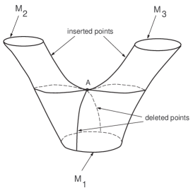
Figure 7: 2 dimensional example of the topology change: $M_{1}$ is an initial space and $M_{2,3}$ are the final spaces which are obtained after some topological surgery. $A$ is the point where the time direction is not determined and the metric becomes singular.

Let us consider three different presentation of $\theta(x)$ operator with scalar and spinor fields.

The first case is

$$W^{ab}(x,y)=\phi(x)\theta^{a}\phi(y)\theta^{b}$$ (13.4)

where $a,b$ are the undotted spinor indices, $\phi(x)$ is the scalar field, $\theta^{a}$ is the Grassman number

$$\theta^{a}\theta^{b}+\theta^{b}\theta^{a}=0.$$ (13.5)

It is easy to proof that

$$\begin{split}W^{ab}(x,y)W_{ab}(x,y)=\phi^{2}(x)\phi^{2}(y)\theta^{a}\theta^{b}\theta_{a}\theta_{b}&=\\ \phi^{2}(x)\phi^{2}(y)\varepsilon_{aa^{\prime}}\varepsilon_{bb^{\prime}}\theta^{a}\theta^{b}\theta^{a^{\prime}}\theta^{b^{\prime}}&\equiv 0\end{split}$$ (13.6)

where

$$\varepsilon^{ab}=\begin{pmatrix}0&1\\ -1&0\end{pmatrix},\qquad\varepsilon_{ab}=\begin{pmatrix}0&-1\\ 1&0\end{pmatrix}.$$ (13.7)

The second case is

$$\begin{split}W(x,y)=\psi_{a}(x)\theta^{a}\psi_{b}(y)\theta^{b}=\psi_{a}(x)\psi_{b}(y)\theta^{a}\theta^{b}&=\\ \left(\psi_{1}(x)\psi_{2}(y)-\psi_{2}(x)\psi_{1}(y)\right)\theta^{1}\theta^{2}&\end{split}$$ (13.8)

where $\psi_{a}(x)$ is an undotted spinor field in $(\frac{1}{2},0)$ representation. The square is zero

$$W^{2}(x,y)=\left(\psi_{1}(x)\psi_{2}(y)-\psi_{2}(x)\psi_{1}(y)\right)^{2}\theta^{1}\theta^{2}\theta^{1}\theta^{2}\equiv 0.$$ (13.9)

In this case $W(x,x)\equiv 0$. It means that the minimalist wormhole can connect only two different points.

The same can be written for $(0,\frac{1}{2})$ representation.

The third case is

$$W(x,y)=\psi_{a}(x)\theta^{a}\psi_{\dot{b}}(y)\bar{\theta}^{\dot{b}}=\psi_{a}(x)\psi_{\dot{b}}(y)\theta^{a}\bar{\theta}^{\dot{b}}$$ (13.10)

where $\psi_{\dot{b}}$ is a dotted spinor in $(0,\frac{1}{2})$ representation. The square is zero

$$\begin{split}W^{2}(x,y)=\left(\psi_{a}(x)\psi_{\dot{b}}(y)\theta^{a}\bar{\theta}^{\dot{b}}\right)\left(\psi_{c}(x)\psi_{\dot{d}}(y)\theta^{c}\bar{\theta}^{\dot{d}}\right)&=\\ \Bigl{(}\psi_{a}(x)\psi_{c}(x)\theta^{a}\theta^{c}\Bigr{)}\left(\psi_{\dot{b}}(y)\psi_{\dot{d}}(y)\bar{\theta}^{\dot{b}}\bar{\theta}^{\dot{d}}\right)&\equiv 0\end{split}$$ (13.11)

as

$$\psi_{a}(x)\psi_{c}(x)\theta^{a}\theta^{c}=\psi_{1}(x)\psi_{2}(x)\theta^{1}\theta^{2}+\psi_{2}(x)\psi_{1}(x)\theta^{2}\theta^{1}\equiv 0.$$ (13.12)

The third case is more interesting because it has both dotted and undotted spinors. We have to note that as the classical canonical theory cannot describes topology change these operators do not correspond to any classical observables. It corresponds to the well-known fact that the Grassman numbers do not have any classical interpretation.

We can suppose that $W(x,y)$ operator is described with dynamical fields : scalar field $\phi(x)$ or spinor field $\psi(x)$. The problem here is what kind of equations we have to apply for the definition of $\phi/\psi$ dynamic ?

The operator $W(x,y)$ can be connected with an indefiniteness (the loss of information) of our knowledge about two points $x^{\mu}$ and $y^{\mu}$ : we do not know if these points are connected by the quantum minimalist wormhole or not. The physical sense of $W(x,y)$ operator is that

$$W(x,y)\approx 0\quad\text{for}\quad|x-y|>l_{0}$$ (13.13)

where $l_{0}$ is some characteristic length depending on some external conditions. For example, for the ordinary spacetime foam without any strong external fields $l_{0}=l_{Pl}=10^{-33}cm$. But in the presence of an external electric field $l_{0}$ can be changed as quantum wormholes can entrap the force lines of electric field.

Let us introduce (following to Smolin) an infinitesimal operator $\delta B(x^{\mu}\rightarrow{x^{\prime}}^{\mu})$ of a displacement of the wormhole mouth

$$\delta B\biggl{(}\theta^{a}\rightarrow{(\theta^{a})}^{\prime},\bar{\theta}^{\dot{a}}\rightarrow{(\bar{\theta}^{\dot{a}})}^{\prime},x^{\mu} \rightarrow {x^{\prime}}^{\mu}\biggl{)}W(y^{\mu},x^{\mu})=W(y^{\mu},{x^{\prime}}^{\mu}),$$ (13.14)

$$W(y^{\mu},x^{\mu}) = \psi_{a}(y^{\mu})\psi_{\dot{b}}(x^{\mu})\theta^{a}\bar{\theta}^{\dot{b}},$$ (13.15)

$$W(y^{\mu},{x^{\prime}}^{\mu}) = \psi_{a}(y^{\mu})\psi_{\dot{b}}({x^{\prime}}^{\mu})\left(\theta^{a}+\varepsilon^{a}\right)\left(\bar{\theta}^{\dot{b}}+\bar{\varepsilon}^{\dot{b}}\right)$$ (13.16)

here $\varepsilon^{\alpha},\bar{\varepsilon}^{\dot{b}}$ is infinitesimal Grassmannian numbers. Therefore we have the following equation for the definition of $\delta B(z^{A}\rightarrow{z^{\prime}}^{A})$ operator (here $z^{A}=\{x^{\mu},\theta^{a},\bar{\theta}^{\dot{b}}\}$ is the coordinates on a superspace)

$$\delta B\left(z^{A}\rightarrow{z^{\prime}}^{A}\right)\psi_{a}(y^{\mu})\psi_{\dot{b}}(x^{\mu})\theta^{a}\bar{\theta}^{\dot{b}}=\psi_{a}(y^{\mu})\psi_{\dot{b}}({x^{\prime}}^{\mu})\left(\theta^{a}+\varepsilon^{a}\right)\left(\bar{\theta}^{\dot{b}}+\bar{\varepsilon}^{\dot{b}}\right).$$ (13.17)

This equation has the following solution

$$\delta B\left(z^{A}\rightarrow{z^{\prime}}^{A}\right)=1+\varepsilon^{\alpha}\frac{\partial}{\partial\theta^{\alpha}}-i\varepsilon^{\alpha}\sigma^{\mu}_{\alpha\dot{\beta}}\bar{\theta}^{\dot{\beta}}\partial_{\mu}+\bar{\varepsilon}^{\dot{\alpha}}\frac{\partial}{\partial\bar{\theta}^{\dot{\alpha}}}+i\theta^{\alpha}\sigma^{\mu}_{\alpha\dot{\beta}}\bar{\varepsilon}^{\dot{\beta}}\partial_{\mu}$$ (13.18)

For the proof of Eq. (13.18) we shall calculate the effect of the $\delta B$ operator on the $W(y^{\mu},x^{\mu})$ operator. On the one hand we have

$$\begin{split}&\delta B\left(z^{A}\rightarrow{z^{\prime}}^{A}\right)W\left(y^{\mu},x^{\mu}\right)=\\ &\biggl{(}1+\varepsilon^{\alpha}\frac{\partial}{\partial\theta^{\alpha}}-i\varepsilon^{\alpha}\sigma^{\mu}_{\alpha\dot{\beta}}\bar{\theta}^{\dot{\beta}}\partial_{\mu}+\bar{\varepsilon}^{\dot{\alpha}}\frac{\partial}{\partial\bar{\theta}^{\dot{\alpha}}}+i\theta^{\alpha}\sigma^{\mu}_{\alpha\dot{\beta}}\bar{\varepsilon}^{\dot{\beta}}\partial_{\mu}\biggl{)}\psi_{a}(y^{\mu})\psi_{\dot{b}}(x^{\mu})\theta^{a}\bar{\theta}^{\dot{b}}=\\ &\psi_{a}(y^{\mu})\psi_{\dot{b}}(x^{\mu})\theta^{a}\bar{\theta}^{\dot{b}}+\psi_{a}(y^{\mu})\psi_{\dot{b}}(x^{\mu})\varepsilon^{a}\bar{\theta}^{\dot{b}}+\psi_{a}(y^{\mu})\psi_{\dot{b}}(x^{\mu})\theta^{a}\bar{\varepsilon}^{\dot{b}}+\\ &\psi_{a}(y^{\mu})\psi_{\dot{b}}(x^{\mu})\delta x^{\mu}\theta^{a}\bar{\theta}^{\dot{b}}\approx\psi_{a}(y^{\mu})\psi_{\dot{b}}(x^{\mu})\left(\theta^{a}+\varepsilon^{a}\right)\left(\bar{\theta}^{\dot{b}}+\bar{\varepsilon}^{\dot{b}}\right)+\\ &\psi_{a}(y^{\mu})\psi_{\dot{b}}(x^{\mu})\delta x^{\mu}\theta^{a}\bar{\theta}^{\dot{b}}\end{split}$$ (13.19)

where

$$\delta x^{\mu}=-i\varepsilon^{\alpha}\sigma^{\mu}_{\alpha\dot{\beta}}\bar{\theta}^{\dot{\beta}}+i\theta^{\alpha}\sigma^{\mu}_{\alpha\dot{\beta}}\bar{\varepsilon}^{\dot{\beta}}.$$ (13.20)

On the other hand

$$\begin{split}&\delta B\left(z^{A}\rightarrow{z^{\prime}}^{A}\right)W\left(y^{\mu},x^{\mu}\right)=\psi_{a}(y^{\mu})\psi_{\dot{b}}(x^{\mu}+\delta x^{\mu})\left(\theta^{a}\right)^{\prime}\left(\bar{\theta}^{\dot{b}}\right)^{\prime}=\\ &\psi_{a}(y^{\mu})\psi_{\dot{b}}(x^{\mu})\left(\theta^{a}\right)^{\prime}\left(\bar{\theta}^{\dot{b}}\right)^{\prime}+\psi_{a}(y^{\mu})\psi_{\dot{b}}(x^{\mu})\delta x^{\mu}\theta^{a}\bar{\theta}^{\dot{b}}\end{split}$$ (13.21)

where $\left(\theta^{a}\right)^{\prime}=\theta^{a}+\epsilon^{a}$ and $\left(\bar{\theta}^{\dot{b}}\right)^{\prime}=\bar{\theta}^{\dot{b}}+\bar{\epsilon}^{\dot{b}}$. We see that r.h.s. of Eq’s (13.19) and (13.20) coincide. It means that the operator $W^{\gamma\delta}(y^{\mu},{x^{\prime}}^{\mu})$ with the shifted wormhole mouth is equivalent to the shift of the coordinates in superspace $z^{A}\rightarrow{z^{\prime}}^{A}$.

After this we can say that $\theta=\{\theta^{\alpha},\theta^{\dot{\alpha}}\}$ are the Grassmanian numbers which we should use as some additional coordinates for the description of the spacetime foam.

Such approach can give us an excellent possibility for understanding of geometrical meaning of spin-$\hbar/2$. Wheeler [9] has mentioned repeatedly the importance of a geometrical interpretation of spin-$\hbar/2$. He wrote: the geometrical description of $\hbar/2$-spin must be a significant component of any electron model.

14 Geometrical interpretation

In this approach superspace is a model of the spacetime foam in quantum gravity. The indefiniteness connected with the creation/annihilation of quantum minimalist wormholes is described by Grassmannian coordinates (see, Fig.8). In this interpretation an infinitesimal Grassmannian coordinate transformation is associated with a displacement of the wormhole mouth, i.e. with a change of the identification procedure (see, Fig.8)

$$\theta^{\prime}=\theta+\varepsilon=Id\biggl{(}y^{\mu}\;\raisebox{6.45831pt}{$\underleftrightarrow{\scriptstyle{\;\;yes\;or\;no\;?\;\;}}$}\;{x^{\prime}}^{\mu}=\\ x^{\mu}-i\varepsilon^{\alpha}\sigma^{\mu}_{\alpha\dot{\beta}}\bar{\theta}^{\dot{\beta}}+i\theta^{\alpha}\sigma^{\mu}_{\alpha\dot{\beta}}\bar{\varepsilon}^{\dot{\beta}}\biggl{)}=W\left(y^{\mu},{x^{\prime}}^{\mu}\right)$$ (14.1)

here the identification procedure $Id(\ldots)$ is described by the operator $W\left(y^{\mu},{x^{\prime}}^{\mu}\right)$. In this case the Grassmannian coordinate transformation has a very clear geometrical sense : it describes a displacement of the wormhole mouth or it is the change of the identification prescription. It is necessary to note that in Ref. [10] there is a similar interpretation of the Grassmanian ghosts : they are the Jacobi fields which are the infinitesimal displacement between two classical trajectories.

In this geometrical approach supersymmetry means that a supersymmetrical Lagrangian is invariant under the identification procedure (13.1), i.e. the corresponding supersymmetrical fields must be described in an invariant manner on the background of the spacetime foam.

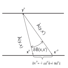
Figure 8: The distinction between two identification prescriptions $\theta$ and $\theta^{\prime}$ leads to a displacement $\delta x^{\mu}=-i\varepsilon^{\alpha}\sigma^{\mu}_{\alpha\dot{\beta}}\bar{\theta}^{\dot{\beta}}+i\theta^{\alpha}\sigma^{\mu}_{\alpha\dot{\beta}}\bar{\varepsilon}^{\dot{\beta}}$

15 Fermionic degrees of freedom on the $\Delta-$string

The fermionic degrees of freedom can appear on the $\Delta-$string if we suppose that quantum gravity play an essential role on the $\Delta-$string. It is the natural assumption because the cross section of the $\Delta-$string is in Planck region. It means that the spacetime foam should give rise to an essential contribution for the consideration of the $\Delta-$string characteristics. Taking into account the presence of quantum wormholes of spacetime foam one can imagine the $\Delta-$string as a shaggy $\Delta-$string, see Fig. 9.

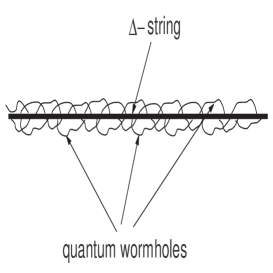
Figure 9: The shaggy $\Delta-$string dressed with quantum minimalist wormholes which can be described by a fermion field.

Taking into account Smolin’s idea about connection between fermions and topology (minimalist quantum wormholes in spacetime foam) one can suppose that spacetime foam on the $\Delta-$string generates fermionic degrees of freedom and the reasonongs similar to Section 13 will lead to an object which is similar to superstrings in string theory.

The problem here is that we should determine what kind of the dynamic (Lagrangian) we should use for spinor field $\psi$ in Eq’s (10.4) (13.10) ? According to Section 14 it can be supergravity where we have gravitation, gauge fields and their fermionic partners. In this approach one can investigate gravitational flux tube solutions with the presence of fermionic fields. Unfortunatelly in supergravity the solutions with spinor fields almost are unknown. Evidently it is connected with mathematical problems of the corresponding Rarita-Schwinger equation. Thus it can be the problem for the future investigations.

16 Conclusions

In this letter we have considered the gravitational flux tube solutions in 5D Kaluza-Klein gravity. These solutions are labeled by the relation between electric and magnetic fields. We have shown that in the case $E\approx H$ (with $E>H$) the corresponding spacetime has a part which is like to a flux tube filled with the electric and magnetic fields. Such tube can be arbitrary thin and long. It allows us to call such superthin and superlong tubes as a string-like objects, namely a $\Delta-$string. We have shown that taking into account the infinitesimal of the cross section (which is in the Planck region) one can reduce 5D initial degrees of freedom to 2D degrees of freedom living on the $\Delta-$string. The corresponding equations describe the propagation of scalar and gauge fields through the $\Delta-$string. It is necessary to note that 2D dynamic on the $\Delta-$string differs from the dynamic of the ordinary string in string theory. The reason is very simple: $\Delta-$string has non-zero cross section.

On the $\Delta-$string one can introduce fermionic degrees of freedom if we take into account such phenomena in quantum gravity as spacetime foam. According to Smolin the quantum wormholes can be connected with a fermion field which describes minimalist wormholes as it presented in Section 13, 14. In this model every quantum wormhole of spacetime is a short $\Delta-$string attached to an external spacetime, see Fig. 10. In such scenario quantum wormholes (or Smolin’s minimalist wormholes) are described by a fermion field. According to Sections 13, 14 these fermion fields are fermion ingredients of some supergravity theory.

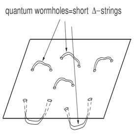
Figure 10: .

17 Acknowledgment

I am very grateful to the ISTC grant KR-677 for the financial support.

References

[1]
V. Dzhunushaliev and D. Singleton, Phys. Rev. D59,
064018 (1999).
[2]
T. Levi-Civita,
Atti Acad. Naz. Lincei, 26, 519 (1917) ;
B. Bertotti,
Phys. Rev., 116, 1331 (1959);
I. Robinson,
Bull. Akad. Pol., 7, 351 (1959).
[3]
J. M. Overduin and P. S. Wesson, Phys. Rept., 283, 303 (1997).
[4]
R. Coquereaux and A. Jadczyk, Commun. Math. Phys. 90, 79 (1983).
[5]
L. Smolin, “Fermions and topology”, gr-qc/9404010.
[6]
Morris W. Hirsch, ”Differential topology“, (Springer-Verlag,
New-York-Heidelberg-Berlin, 1976).
[7]
V. Dzhunushaliev, Found. Phys., 32, 1069 (2002).
[8]
J. L. Friedman and R. D. Sorkin,
Phys. Rev. Lett. 44 (1900) 1100; Gen. Rel and Grav. 14
(1982) 615.
[9]
J.Wheeler, Neutrinos, Gravitation and Geometry
(Princeton Univ. Press, 1960).
[10]
E. Gozzi, M. Reuter and W. D. Tacker, Phys. Rev.,
D40, 3363(1989).