On the origin of the matter-antimatter asymmetry in self-gravitating systems at ultra-high temperatures

Abstract

It is shown, that self-gravitating systems can be classified by a dimensionless constant positive number $\kappa=ST/E$, which can be determined from the (global) values for the entropy, temperature and (total) energy. The Kerr-Newman black hole family is characterized by $\kappa$ in the range $0-1/2$, depending on the dimensionless ratios of angular momentum and charge squared to the horizon area, $J/A$ and $Q^{2}/A$.

By analyzing the most general case of an ultra-relativistic ideal gas with non-zero chemical potential it is shown, that $\kappa$ is an important parameter which determines the (local) thermodynamic properties of an ultra-relativistic gas. $\kappa$ only depends on the chemical potential per temperature $u=\mu/T$ and on the ratio of bosonic to fermionic degrees of freedom $r_{F}=f_{B}/f_{F}$. A gas with zero chemical potential has $\kappa=4/3$. Whenever $\kappa<4/3$ the gas must acquire a non-zero chemical potential. This non-zero chemical potential induces a natural matter-antimatter asymmetry, whenever microscopic statistical thermodynamics can be applied.

The recently discovered holographic solution describes a compact self gravitating black hole type object with an interior, well defined matter state. One can associate a local - possibly observer-dependent - value of $\kappa$ to the interior matter, which lies in the range $2/3-1$ (for the uncharged case). This finding is used to construct an alternative scenario of baryogenesis in the context of the holographic solution, based on quasi-equilibrium thermodynamics.

1 Introduction

In our universe we experience a profound matter-antimatter asymmetry. It’s fundamental origin is not known. The standard explanation for this asymmetry is attributed to the dynamic evolution of the universe shortly after the ”big-bang”. According to the mechanism first sketched out by Sacharov already in the year 1967 [14], a CP-violating process taking place at high temperatures (such as the asymmetric decay of the $X$ and $Y$ bosons below the GUT-scale) combined with a temporary deviation from thermal equilibrium, as could have been caused by the rapid expansion of the universe, can transform a slight matter-antimatter asymmetry at high temperatures into a profound asymmetry at low temperatures.

The low baryon to photon ratio of $\eta\approx 10^{-9}$ encountered in our universe in its present state is usually interpreted as a remnant of a former minuscule asymmetry in the baryon-antibaryon-number of the order of $10^{-9}$. According to the common belief there were roughly $10^{9}+1$ baryons vs. $10^{9}$ antibaryons at the time, when the temperature of the universe fell below the rest-mass of the nucleon. The baryons/antibaryons annihilated at this threshold, predominantly into photons, leaving 1 baryon and $10^{9}$ photons behind. This primordial ratio of $10^{9}$ photons per baryon then was preserved - at least approximately - during the subsequent expansion.

Although such a scenario is thinkable, in the sense that it doesn’t appear to be in direct contradiction to any fundamental physical laws, and is furthermore supported by (indirect) experimental evidence such as today’s high value for the photon to baryon ratio which appears to fit well with the ratio predicted from primordial nucleosynthesis, the scenario relies on several implicit assumptions, which appear questionable.

The first assumption is, that our universe is accurately described by a homogeneous Friedman Robertson Walker (FRW) model, over the full temperature range from the GUT-energy-breaking scale to the low energy scale today. This assumption has been quite successful in explaining many of the phenomena encountered in the observable universe today in terms of a solution of the field equations of only moderate mathematical complexity. On the other hand, today’s standard cosmological has lost much of its original charm. It has turned into a complex model, relying on the experimental determination of several crucial parameters (such as the fraction of cold dark matter, dark energy) whose numerical values cannot be predicted by today’s methods and whose fundamental origin is not known. There is no theorem that the universe must be describable by an FRW-model. In fact, the so called holographic solution, an exact solution to the Einstein-field equations with zero cosmological constant, was shown to be a potential alternative model for the universe [11] . In contrast to the FRW-model the holographic solution has no free parameters. Yet it’s unique properties fit today’s observational facts very well. But its evolution very much differs from that of a FRW-universe.

The second assumption is tied to the first. The standard scenario of big-bang baryogenesis makes heavy use of the argument, that in a homogeneously expanding FRW-type universe the particle numbers of the different species in a co-moving volume-element should remain constant during the expansion. This assumption is model-dependent. Although it is true in the FRW-model, it can fail in other models. In the holographic solution the baryon to photon ratio is time dependent and evolves linearly with temperature.

The third assumption is about the nature of the phase-transition at the time of baryogenesis. The implicit assumption in the standard cosmological model is, that the phase transition caused a vast imbalance in particle numbers almost instantly: If one compares the temperature-dependencies of the particle interaction rates with the Hubble rate, one can conclude quite confidently that the very early universe must have been in thermodynamic equilibrium. This means, that the number- and energy-densities of all known particle species, such as baryons and photons, must have been roughly equal at the time slightly before baryogenesis. Slightly after baryogenesis the standard cosmological model, however, postulates a discrepancy in the energy- and number-densities of photons and (left over) nucleons of the order of $10^{9}$. This extreme imbalance in particle numbers then is assumed to have been preserved throughout the whole intermediate energy range up to nucleosynthesis and beyond, down to the low temperatures encountered today.

The justification for this type of phase transition is, that it provides a plausible explanation for the profound matter anti-matter asymmetry in our universe at low temperatures, if one assumes a minuscule asymmetry at high temperatures (as the high ratio of photons to baryons observed today seems to imply). Unfortunately there is no mechanism which comes close to explain the small primordial asymmetry of order $10^{-9}$. As long as this crucial assumption, which lies at the heart of the matter anti-matter problem, has not found a satisfactory theoretical explanation, it is worthwhile to explore alternatives.

In this paper I attempt to give an alternative explanation for the matter-antimatter asymmetry, which is based on equilibrium thermodynamics of an ultra-relativistic gas of fermions and bosons. The crucial observation is, that whenever the ultra-relativistic fermions develop a non-zero chemical potential comparable to the temperature, this can act as a natural - purely thermodynamic - cause for a profound matter-antimatter asymmetry at high temperatures.

That a non-zero chemical potential induces a matter-antimatter asymmetry is a well known fact from microscopic statistical thermodynamics. The question is, under what circumstances such a non-zero chemical potential can arise. It turns out that self-gravitating systems, which are characterized by the property that their entropy can be expressed as a function of the energy alone, i.e. $S=S(E)$, provide a natural setting for a non-zero chemical potential of the fermions at ultra-relativistic temperatures. Such systems are characterized by a strict proportionality between the total energy and the free energy $F=(1-\kappa)E$. The constant value of $\kappa$ can only take on a very narrow range: $0<\kappa\leq 4/3$. The standard case of an ultra-relativistic gas with zero chemical potential is described by $\kappa=4/3$. Whenever $\kappa\neq 4/3$, non-zero values for the chemical potentials of the fermions necessarily arise. Classical black holes have values of $\kappa$ in the range $0<\kappa\leq 1/2$ ($\kappa=1/2$ for a Schwarzschild black hole, $\kappa\rightarrow 0$ for an extreme Kerr-Newman black hole). An interesting value is $\kappa=1$, which is realized within the holographic solution. For $\kappa=1$ the free energy is minimized to zero.

The question, by what physical process the non-zero chemical potentials of the fermions can arise in the first place, will not be answered in this paper. It seems clear, that one requires some (local) violation of $CP$ and/or $P$. In order to save the $CPT$-theorem $T$ would have to be violated locally as well. The weak interactions are known to violate $P$ maximally. $CP$ is violated in certain weak decay processes. Quite interestingly, the rotating holographic solution appears to provide a natural setting for a significant local $CP$-violation of the macroscopic state, if the interior ultra-relativistic particles (such as neutrinos or anti-neutrinos) are aligned along the direction of the exterior rotation axis. See [12] for more details.

The paper is divided into five principal sections. In section 2 the thermodynamic properties of the most general case of an ultra-relativistic gas of fermions and bosons is discussed. A relation between the chemical potential per temperature of the gas and the dimensionless ratio $\kappa=ST/E$ of the system will be derived. In section 3 I will discuss the relation between energy and entropy for several self-gravitating systems and will demonstrate, how the dimensionless ratio $\kappa$ determines the global and local properties of the system. In section 4 necessary conditions are discussed, under which an ultra-relativistic gas can develop a non-zero chemical potential. In section 5 the findings of the previous sections will be discussed for for some particular self-gravitating systems. Section 6 then describes an alternative scenario for the origin of the matter-antimatter asymmetry, using the holostar solution as a simple model.

2 Thermodynamics of an ultra-relativistic gas of fermions and bosons

The objective of this section is to derive the thermodynamic properties for the most general case of an ultra-relativistic ideal gas consisting out of bosons and fermions. Most of the explicit derivations will be done for fermions. The results then are extended for the more general case of a gas consisting out of bosons, fermions and anti-fermions.

2.1 General properties of an ultra-relativistic ideal gas

An ultra-relativistic gas must be described by the grand canonical ensemble: At ultra-relativistic temperatures we will have copious particle-interchange reactions between the different particle species. Each species exchanges particles, energy and entropy with the other species. The number of particles within any given species cannot be considered fixed, but rather has to adjust to the thermodynamic constraints.

Let us assume, that the time-scale of the interaction processes is small enough so that thermal equilibrium can be attained, yet that the interactions are weak enough so that the gas can be described - at least approximately - as an ideal gas of massless, essentially non-interacting particles. These assumptions should be valid at the high temperatures and densities encountered in the very early universe.

Under the ideal gas assumption the contribution of the individual particle species to the extrinsic quantities, such as entropy and energy, can be calculated separately. The total for each (extrinsic) quantity is formed just by summing up the individual contributions.

I will first consider a gas consisting only out of fermions. The bosons, anti-bosons and anti-fermions will be added later. This only changes some numerical factors, not the general picture. For convenience units $c=1$ will be used throughout this paper.

A gas at ultra-high temperatures is expected to consist exclusively out of elementary (i.e. not composed) particles. The main characteristics, by which elementary particles can be distinguished from each other are mass, spin and charge(s). At ultra-high temperatures some of the characteristic features distinguishing different particle species from each other will become blurred: The particles will act more and more like truly massless particles, the higher the temperature becomes. At ultra-high energies the particle’s rest mass is an utterly insignificant correction to the energy-momentum relation $E\simeq p$. The actual value of the spin of a particle doesn’t play a significant role at ultra-high temperatures either, as all transverse spin-directions are heavily suppressed. We might be able to distinguish the particles by their different charges. However, if the $GUT$-picture is correct, all known charges (electro-weak, strong) will unify at some high energy, so that the charge looses it’s distinguishing quality at high energies. Furthermore the fine-structure constant, as well as the other coupling constants, are expected to remain small, even at the Planck energy, so that the electric charge - as well as the other charges - only provide a very moderate correction to the ideal gas law. If the gas is neutral, the charge(s) of the particles most likely will be quite irrelevant for the thermodynamic properties of a gas at ultra-high temperatures.

Therefore, at energies well above the electro-weak scale it is not unreasonable to assume that the particles are only distinguished by the different representations of the Poincare-group for a massless particle. The only label of a (non-tachyonic) particle in the massless sector of the Poincare-group is the particle’s helicity. If the macroscopic state of the system does not single out a preferred axis (no rotation), the spin of a particle is only relevant to the thermodynamic description in the sense, that the two opposite spin-components provide separate degrees of freedom that must be included in the counting of the fundamental degrees of freedom.

Therefore the only relevant microscopic parameter describing a neutral, isotropic gas of ultra-relativistic fermions in thermodynamic equilibrium should be the number of degrees of freedom of the fermions. Let us denote this number by $f_{F}$.

However, we also have to consider the macroscopic thermodynamic parameters. Therefore we cannot rule out the possibility that the fermions have a non-zero chemical potential. If this happens to be the case, it is reasonable to conjecture that all fermionic species have the same chemical potential at ultra-relativistic energies: The chemical potential is a measure of how much energy must be invested to add a new particle to a closed system, without changing its entropy or volume $\mu=(\partial E/\partial N)_{S,V}$. At ultra-high temperatures, where the rest-masses, charges etc. of the fermions are utterly negligible, the energy required to add a new particle to the gas is expected to be only a (linear) function of temperature, quite independent of the nature of the particle.

Let us denote the ratio of the fermionic chemical potential to the temperature by $u=\mu_{F}/T$. According to the above discussion an ultra-relativistic gas of fermions will be fully described by just two dimensionless parameters: the number of fermionic degrees of freedom $f_{F}$ and the chemical potential per temperature $u$.

2.2 The grand canonical formalism and some important abbreviations

We now proceed to determine the thermodynamic properties of an ultra-relativistic gas of fermions. The relevant quantity in the grand-canonical formalism is the grand canonical potential $J(T,\mu,V)$, which is defined as a function of temperature $T$, chemical potential $\mu$ and volume $V$. For an ultra-relativistic gas with $f_{F}$ fermionic degrees of freedom with energy-momentum relation $\epsilon=p$ the grand canonical potential is given by:

$$J(T,\mu,V)=-\frac{f_{F}}{(2\pi\hbar)^{3}}T\,V\int\int\int d^{3}p\,\ln{(1+e^{-\frac{p-\mu}{T}})}$$ (1)

By introducing the dimensionless integration variable $z=p/T$ we can cast $J$ into another form:

$$J=-T^{4}V\frac{f_{F}}{2\pi^{2}\hbar^{3}}\int_{0}^{\infty}{z^{2}\ln{(1+e^{-z+u})}dz}$$ (2)

where we have set the integration ranges to zero and infinity and replaced the chemical potential per temperature with the dimensionless parameter $u$:

$$u=\frac{\mu}{T}$$ (3)

$u$ depends on $\mu$ and $T$, which are both independent variables in the grand canonical formalism. Therefore, whenever we calculate the thermodynamic quantities from the grand-canonical potential via partial derivatives, we must treat $u$ as a function of the independent variables $\mu$ and $T$.

The integral in equation (2) can be transformed to the following integral by a partial integration:

$$J=-T^{4}V\frac{f_{F}}{2\pi^{2}\hbar^{3}}\frac{1}{3}\int_{0}^{\infty}{z^{3}n_{F}(z,u)dz}$$ (4)

where $n_{F}$ is the mean occupancy number of the fermions:

$$n_{F}(z,u)=\frac{1}{e^{z-u}+1}=\frac{1}{e^{\frac{p-\mu}{T}}+1}$$ (5)

The thermodynamic equations for an ideal gas at ultra-relativistic temperature can be expressed exclusively in terms of definite integrals, whose integrand contains $n_{F}$ multiplied by an integer power of $z$. I will denote these integrals by $Z_{F,n}$:

$$Z_{F,n}(u)=\int_{0}^{\infty}{z^{n}n_{F}(z,u)dz}$$ (6)

Such integrals can be evaluated by the poly-logarithmic function (see the Appendix for specific formula).

2.3 Extrinsic quantities and densities

According to the grand canonical formalism the entropy $S$ can be calculated by a partial differentiation with respect to $J$:

$$S=-\frac{\partial J}{\partial T}=\frac{f_{F}}{2\pi^{2}\hbar^{3}}T^{3}V\left(\frac{4}{3}Z_{F,3}(u)-uZ_{F,2}(u)\right)$$ (7)

For the derivation of the entropy the following identity has been used:

$$\frac{\partial{Z_{F,3}(u)}}{\partial x}=3Z_{F,2}(u)\frac{\partial u}{\partial x}$$ (8)

The pressure is given by:

$$P=-\frac{\partial J}{\partial V}=\frac{f_{F}}{2\pi^{2}\hbar^{3}}\frac{Z_{F,3}(u)}{3}T^{4}=\frac{F_{E}}{3}T^{4}$$ (9)

where the following abbreviation was used:

$$F_{E}=\frac{f_{F}Z_{F,3}(u)}{2\pi^{2}\hbar^{3}}$$ (10)

With the above relation, the grand canonical potential $J$ can be expressed in terms of $P$ and $V$:

$$J=-\frac{F_{E}}{3}VT^{4}=-PV$$ (11)

The entropy $S$ can be expressed as:

$$S=F_{S}T^{3}V$$ (12)

with

$$F_{S}=\frac{f_{F}\left(\frac{4}{3}Z_{F,3}(u)-uZ_{F,2}(u)\right)}{2\pi^{2}\hbar^{3}}$$ (13)

The total energy is calculated from the grand canonical potential via:

$$E=J-\left(T\frac{\partial}{\partial T}+\mu\frac{\partial}{\partial\mu}\right)J=\frac{f_{F}}{2\pi^{2}\hbar^{3}}T^{4}VZ_{F,3}(u)=F_{E}T^{4}V$$ (14)

As expected, we find the equation of state for an ideal ultra-relativistic gas:

$$e=\frac{E}{V}=3P$$

Throughout this paper the extrinsic quantities, such as total energy $E$, total entropy $S$ etc. of a space-time region $V$ will be denoted by capital letters, whereas the densities will be denoted by lower case letters. Quantities referring to the properties of the individual particles, such as the mean energy per particle or the entropy per particle will be denoted by (lower case) greek letters. With this notation the total energy is denoted by $E$, the energy-density by $e$ and the energy per particle by $\epsilon$.

The grand-canonical potential $J$ is related to the total energy via the well-known relation:

$$J=-\frac{E}{3}$$

Keep in mind that $J$ is defined as a function of $T$, $V$ and $\mu$, so that taking a partial derivative with respect to $E$ is tricky.

The energy-density $e=E/V$ is proportional to the fourth power of the temperature and proportional to the number of ultra-relativistic degrees of freedom, via $f_{F}$:

$$e=\frac{E}{V}=F_{E}T^{4}$$

Combining equations (12, 14) we can derive a relation between the entropy, the energy and the temperature:

$$ST=\frac{F_{S}}{F_{E}}E=\kappa E$$ (15)

The ratio of $F_{S}/F_{E}$ will turn out important later, so we have denoted it by $\kappa$:

$$\kappa=\frac{ST}{E}=\frac{F_{S}}{F_{E}}$$ (16)

Note that according to equation (16) $\kappa$ is defined exclusively in terms of the thermodynamic quantities $S$, $T$ and $E$. This definition of $\kappa$ is completely general. It appears, as if $\kappa$ can take on any (non-zero) value. However, for most systems $\kappa$ is of order unity and nearly constant. Take for example an ideal gas of massive particles at low temperature. For $m\gg T$ the entropy per massive particle is $\sigma\approx m/T$ and the total energy per particle is $\epsilon=m+3/2\,T$, so that $\kappa\rightarrow 1$. For any Kerr-Newman black hole with given angular momentum and charge $\kappa$ is constant, and lies in the range $0<\kappa\leq 1/2$ (see section 3.3).

For an ultra-relativistic gas $\kappa=F_{S}/F_{E}$, which is of order unity and nearly constant whenever the number of particle degrees of freedom does not change. For a gas consisting exclusively out of fermions $\kappa$ only depends on $u$, but not on the number of fermionic degrees of freedom $f_{F}$. If the gas has a non-zero contribution of bosons, $\kappa$ also depends - albeit very moderately - on the ratio of bosonic to fermionic degrees of freedom.

The total number of particles is given by:

$$N=-\frac{\partial J}{\partial\mu}=\frac{f_{F}}{2\pi^{2}\hbar^{3}}Z_{F,2}(u)T^{3}V=F_{N}T^{3}V$$ (17)

where we have defined the quantity

$$F_{N}=\frac{f_{F}Z_{F,2}(u)}{2\pi^{2}\hbar^{3}}$$ (18)

Like $F_{E}$ and $F_{S}$, the value of $F_{N}$ only depends on the chemical potential per temperature $u$ and on the number of ultra-relativistic degrees of freedom $f$. When these quantities are fixed, then $F_{E}$, $F_{S}$ and $F_{N}$ are constants.

The number-density $n=N/V$ is proportional to the cube of the temperature and proportional to the number of ultra-relativistic degrees of freedom via $F_{N}$

$$n=\frac{N}{V}=F_{N}T^{3}$$ (19)

We can combine equation (19) with equation (9) in order to obtain a relation, which resembles the ideal gas law:

$$PV=\frac{F_{E}}{3F_{N}}NT=RNT$$ (20)

with

$$R=\frac{F_{E}}{3F_{N}}$$ (21)

In the non-relativistic case $R=1$ (in units $c=k=1$), as will be shown in the Appendix. In the ultra-relativistic case $R$ depends on the ratio of bosonic to fermionic degrees of freedom and on $u$. Yet $R$ remains close to unity for reasonable assumptions with respect to the values of $r=f_{F}/f_{B}$ and $u$. For $u=0$ we get $R_{B}=\pi^{4}/(90\zeta(3))\simeq 0.90039$ for bosons. For fermions the value is higher by the factor $7/6$: $R_{F}=7/6\,R_{B}=7\pi^{4}/(540\zeta(3))\simeq 1.05046$.

2.4 Thermodynamic parameters of individual particles

In this section the thermodynamic parameters which refer to the properties of the individual particles will be derived.

The energy per particle is proportional to $T$, as can be seen by combining equations (14, 17):

$$\epsilon=\frac{E}{N}=\frac{Z_{F,3}(u)}{Z_{F,2}(u)}\,\,T=\frac{F_{E}}{F_{N}}\,\,T$$ (22)

The energy per particle depends linearly on the temperature, quite as expected for an ultra-relativistic gas. The constant of proportionality $F_{E}/F_{N}$ doesn’t depend on the number of degrees of freedom (for a gas consisting exclusively out of fermions). It only depends on $u$, the ratio of the chemical potential to the temperature. This ratio might depend indirectly on the temperature. However, as has already been discussed in section 2.1 and as we will see later, $u$ is effectively constant when the number of ultra-relativistic degrees of freedom of the different particle species making up the gas does not change.

The entropy per particle $\sigma$ can be read off from equations (12, 13, 17):

$$\sigma=\frac{S}{N}=\frac{4}{3}\frac{Z_{F,3}(u)}{Z_{F,2}(u)}-u=\frac{F_{S}}{F_{N}}$$ (23)

Similar to the ratio $\epsilon/T=F_{E}/F_{N}$ the entropy per particle $\sigma=F_{S}/F_{N}$ only depends on $u$.

$\sigma$ might be (slightly) temperature-dependent via $u$. Note, however, that for a ”normal” ultra-relativistic gas with non-zero chemical potential we know, that the entropy per particle is constant. For example, a photon gas has $\sigma_{B}\simeq 3.6$ and a gas of massless fermions with zero chemical potential has $\sigma_{F}\simeq 4.2$. Therefore it seems reasonable to assume, that $\sigma$ is nearly constant even in the more general case, where the chemical potential of the fermions is non-zero.

The nearly constant energy per particle per temperature $\epsilon/T$, and the entropy per particle $\sigma$ are related. We find:

$$\sigma=\frac{F_{S}}{F_{E}}\frac{\epsilon}{T}=\kappa\frac{\epsilon}{T}$$ (24)

An interesting case is $\kappa=1$. In such a case the (mean) energy per particle per temperature $\epsilon/T$ is exactly equal to the (mean) entropy per particle $\sigma$. For this particular case the free energy $F$ is exactly zero. $F$ is defined as:

$$F=E-ST$$

If we divide this equation by the particle number $N$, we get the free energy per particle $\phi=F/N$:

$$\phi=\epsilon-\sigma T=(1-\kappa)\epsilon$$

The free energy-density $f=F/V$ follows from the above equation by multiplication with $N/V$:

$$f=e-sT=(1-\kappa)e$$

2.5 Extending the model for bosons

The calculations have been carried through for fermions. The equations for an ultra-relativistic boson gas are very similar to the above equations. We have to replace:

$$n_{F}(z,u)\rightarrow n_{B}(z,u)=\frac{1}{e^{z-u}-1}$$ (25)

$$Z_{F,n}\rightarrow Z_{B,n}=\int_{0}^{\infty}{z^{n}n_{B}(z,u)dz}$$ (26)

For an ideal gas the individual contributions to the extrinsic quantities can be summed up.

2.5.1 The three fundamental parameters of an ultra-relativistic ideal gas: $f_{F}$, $f_{B}$ and $u$

Before we put the bosonic and fermionic contributions together, let us reflect on the fundamental characteristics that will describe the most general case of an ultra-relativistic gas.

Although we won’t be able to distinguish the ultra-relativistic particles by their rest-mass or by the transverse components of their spins, we still should be able to distinguish bosons from fermions. We should also be able to count the different helicity states of a particle (one for a neutrino, two for an electron according to the Standard Model of particle physics). Furthermore, it should be possible to discern the particles in an operational sense, if they have different chemical potentials.

Therefore the only relevant thermodynamic characteristics of a gas consisting of ultra-relativistic fermions and bosons appear to be the respective degrees of freedom of fermions and bosons and their respective chemical potentials. Let us denote the fermionic degrees of freedom by $f_{F}$ and the bosonic degrees of freedom by $f_{B}$.

Generally, i.e. at low energies, the different particle species can have very differing values for the chemical potentials. It is usually assumed that the chemical potential of a non-relativistic particle is related to its rest-mass. There are some restraints. Ultra-relativistic Bosons cannot have a positive chemical potential, as $Z_{B,n}(u)$ is a complex number for positive $u$. Photons and gravitons, in fact all massless gauge-bosons, have a chemical potential of zero, which reflects the fact, that they can be created and destroyed without being restrained by a particle-number conservation law.

Here we are considering a gas of ultra-relativistic particles, where particle-antiparticle pair production will take place abundantly. There will not only be particles around, but every particle will come with its antiparticle. The chemical potentials of a particle and its anti-particle add up to zero: $\mu+\overline{\mu}=0$. This restricts the chemical potential of the bosons: As ultra-relativistic bosons cannot have a positive chemical potential, the chemical potential of any ultra-relativistic bosonic species must be zero, i.e. $\mu_{B}=\overline{\mu_{B}}=0$, whenever the energy is high enough to create boson/anti-boson pairs. This restriction does not apply to the fermions, which can have a non-zero chemical potential at ultra-relativistic energies, as both signs of the chemical potential are allowed. So for ultra-relativistic fermions we can fulfill the relation $\mu_{F}+\overline{\mu_{F}}=0$ with non-zero $\mu_{F}$.

In the following discussion let us take the convention, that any fermion with $\mu_{F}>0$ is classified as ordinary matter, so that all of the anti-fermions have a negative chemical potential. As has been discussed before, it is reasonable to assume that at ultra-high temperatures all fermions will have the same universal value for the chemical potential, which is expected to be proportional to the temperature.

If the fermions have a non-zero chemical potential, we can distinguish bosons from fermions in an operational sense by their different chemical potentials. We don’t have to determine the particle’s spin (integer for bosons, half-integer for fermions).

According to the previous discussion an ideal (uncharged, locally isotropic) gas at ultra-relativistic temperatures is characterized by just three dimensionless numbers: The bosonic and fermionic degrees of freedom $f_{B}$ and $f_{F}$ and the ratio of the chemical potential of the fermions to the temperature, $u=\mu_{F}/T$. Henceforth we will express the thermodynamic properties of the system in terms of these three fundamental parameters.

For many of the following relations it is convenient to replace $f_{F}$ and $f_{B}$ with the ratio of bosonic to fermionic degrees of freedom:

$$r_{f}=\frac{f_{B}}{f_{F}}$$ (27)

and the total number of degrees of freedom

$$f=2(f_{F}+f_{B})$$ (28)

We take the convention here, that $f_{F}$ and $f_{B}$ denote the degrees of freedom of one particle species, including particle and antiparticle. With this convention a photon gas ($g=2$) is described by $f_{B}=1$ (There are two photon degrees of freedom: The photon is its own anti-particle; it comes in two helicity states). All other particle characteristics, such as the different chirality states for a Dirac-electron, are counted extra. The total number of the degrees of freedom in the gas, counting particles and anti-particles separately, will thus be given by $f=2(f_{F}+f_{B})$.

2.5.2 Extending the thermodynamic relations to the general case

We can use all the relations derived for a fermion gas simply by making the following replacements:

$$F_{E}\rightarrow F_{E}(u,f_{F},f_{B})=\frac{f_{F}\left(Z_{F,3}(u)+Z_{F,3}(-u)\right)+2f_{B}Z_{B,3}(0)}{2\pi^{2}\hbar^{3}}$$ (29)

$$F_{N}\rightarrow F_{N}(u,f_{F},f_{B})=\frac{f_{F}\left(Z_{F,2}(u)+Z_{F,2}(-u)\right)+2f_{B}Z_{B,3}(0)}{2\pi^{2}\hbar^{3}}$$ (30)

$$F_{S}\rightarrow F_{S}(u,f_{F},f_{B})=\frac{f_{F}\left(\frac{4}{3}\{Z_{F,3}(u)\}-u[Z_{F,2}(u)]\right)+2f_{B}\frac{4}{3}Z_{B,3}(0)}{2\pi^{2}\hbar^{3}}$$ (31)

For brevity commutator anti-commutator notation was (mis)used:

$$\{Z_{F,n}(u)\}=Z_{F,n}(u)+Z_{F,n}(-u)$$

and

$$[Z_{F,n}(u)]=Z_{F,n}(u)-Z_{F,n}(-u)$$

Once in a while we might want to determine the entropy-, number- and energy-densities of the individual components of the gas, i.e. for a single bosonic or fermionic degree of freedom. In such a case we just have to set $f_{B}$ or $(f_{F},u)$ to zero in the in above defined quantities $F_{E}$, $F_{N}$ and $F_{S}$. For example, in order to obtain the bosonic contributions we set $f_{F}=u=0$; in order to obtain the fermionic contribution (including the fermionic antiparticles) we set $f_{B}=0$. This procedure gives

$$N_{B}=F_{N}(0,0,f_{B})\,\,VT^{3}=\frac{2f_{B}Z_{B,2}(0)}{2\pi^{2}\hbar^{3}}\,\,VT^{3}=f_{B}\frac{2\zeta(3)}{\pi^{2}\hbar^{3}}\,\,VT^{3}$$ (32)

for the number of bosons and

$$N_{F}+\overline{N_{F}}=F_{N}(u,f_{F},0)\,\,VT^{3}=\{F_{N}\}\,\,VT^{3}$$ (33)

for the number of fermions + anti-fermions, where we have defined the quantity

$$\{F_{N}\}=F_{N}(u,f_{F},0)=\frac{f_{F}\left(Z_{F,2}(u)+Z_{F,2}(-u)\right)}{2\pi^{2}\hbar^{3}}$$ (34)

in a somewhat abusive usage of anti-commutator notation.

Calculating the fermionic and anti-fermionic contributions individually is a little bit more tricky. Here we must keep in mind that the fermions are described by the terms with positive $u$ and the anti-fermions with the corresponding negative value $-u$. The number of anti-fermions is given by:

$$\overline{N_{F}}=\frac{f_{F}Z_{F,2}(-u)}{2\pi^{2}\hbar^{3}}\,\,VT^{3}$$ (35)

whereas the number of fermions is obtained by replacing $-u$ with $u$ in the above formula.

The total entropy of the fermions is:

$$S_{F}=\frac{f_{F}\left(\frac{4}{3}Z_{F,3}(u)-uZ_{F,2}(u)\right)}{2\pi^{2}\hbar^{3}}\,\,VT^{3}$$ (36)

For the anti-fermions we have:

$$\overline{S_{F}}=\frac{f_{F}\left(\frac{4}{3}Z_{F,3}(-u)+uZ_{F,2}(-u)\right)}{2\pi^{2}\hbar^{3}}\,\,VT^{3}$$ (37)

For the calculation that follows we will not only need the sum of the number of fermions and anti-fermions, but also their difference:

$$\Delta N_{F}=N_{F}-\overline{N_{F}}=[F_{N}]\,VT^{3}$$ (38)

where again commutator-notation was (ab)used:

$$[F_{N}]=\frac{f_{F}\left(Z_{F,2}(u)-Z_{F,2}(-u)\right)}{2\pi^{2}\hbar^{3}}$$ (39)

The quantity just defined in equation (39) allows us to express $F_{S}$ via $[F_{N}]$ and $F_{E}$:

$$F_{S}=\frac{4}{3}F_{E}-u[F_{N}]$$ (40)

Using the identities known for the poly-log function it is rather easy to show that

$$Z_{F,2}(u)-Z_{F,2}(-u)=\frac{u}{3}\left(\pi^{2}+u^{2}\right)$$ (41)

so that

$$[F_{N}]=\frac{f_{F}}{6\hbar^{3}}\left(1+\frac{u^{2}}{\pi^{2}}\right)u$$ (42)

This allows us to express $u$ as an implicit function of $\Delta n_{F}$, $T$ and $f_{F}$:

$$\frac{\Delta n_{F}}{T^{3}}=\frac{f_{F}}{6\hbar^{3}}\left(1+\frac{u^{2}}{\pi^{2}}\right)u$$ (43)

Another important expression that can be simplified by the known identities for the poly-log function is

$$\frac{Z_{F,3}(u)+Z_{F,3}(-u)}{2Z_{B,3}(0)}+1=\frac{15}{8}\left(1+\frac{u^{2}}{\pi^{2}}\right)^{2}$$ (44)

so that $F_{E}$ can be expressed in a closed form as a function of $u$:

$$F_{E}=\frac{f_{F}\pi^{2}}{15\hbar^{3}}\left(\frac{15}{8}\left(1+\frac{u^{2}}{\pi^{2}}\right)^{2}+(r_{f}-1)\right)$$ (45)

$F_{S}$ can be determined as an explicit function of $u$ via equation (40).

With relations (42, 45) one can determine $u$ in a closed form. Rearranging equation (40) we find

$$\frac{4}{3}-\kappa=\frac{u[F_{N}]}{F_{E}}$$ (46)

Inserting the expressions for $[F_{N}]$ and $F_{E}$ into the above formula we finally get

$$1-\frac{3}{4}\kappa=\frac{\frac{u^{2}}{\pi^{2}}\left(1+\frac{u^{2}}{\pi^{2}}\right)}{\left(1+\frac{u^{2}}{\pi^{2}}\right)^{2}+\frac{8}{15}(r_{f}-1)}$$ (47)

Equation (47) is a quadratic equation in the variable $u^{2}/\pi^{2}$ which is easy to solve. A closed formula will be derived below. It is clear from the above relation that there is only a (real) solution for $u$ if $\kappa\leq 4/3$, because the right hand side of equation (47) is always positive. For $\kappa=4/3$ the only possible value for $u$ is zero, independent of the value of $r_{f}$. If $u$ is a solution, so its negative value $-u$ is a solution as well. Therefore any non-zero value of $u$ allows us to distinguish particles and anti-particles by their respective positive / negative values of $u$.

2.5.3 Fermionic weighting factors

Non-zero $u$ is only possible for fermions. Ultra-relativistic bosons always have $u=0$. Therefore the extrinsic thermodynamic quantities of the bosons, such as number-, energy- and entropy-densities can be calculated by multiplying the values derived from the well known Planck-distribution with the number of bosonic degrees of freedom $f_{B}$. For a gas of massless fermions with zero chemical potential it is common practice to multiply the fermionic degrees of freedom with the so called ”fermionic weighting factors”, which relate the number-, energy-, entropy-densities of a single fermionic degree of freedom to a single bosonic degree of freedom. It is convenient to extend this procedure for non-zero $u$. The weighting factor for the energy density is given by

$$w_{E}(u)=\frac{Z_{F,3}(u)}{Z_{B,3}(0)}$$ (48)

The weighting factor for the number-density is

$$w_{N}(u)=\frac{Z_{F,2}(u)}{Z_{B,2}(0)}$$ (49)

The weighting factor for the entropy-density can be calculated from the two other weighting factors

$$w_{S}(u)=\frac{\frac{4}{3}Z_{F,3}-uZ_{F,2}(u)}{\frac{4}{3}Z_{B,3}(0)}=w_{E}(u)-u\,w_{N}(u)\frac{45\zeta(3)}{2\pi^{4}}$$ (50)

To get the weighting factors for the anti-fermions, which will be denoted by barred quantities, we just have to replace $u$ with $-u$, i.e. $\overline{w_{E}}=w_{E}(-u)$ and $\overline{w_{N}}=w_{N}(-u)$. For $u=0$ we get the well known factors $7/8$ and $3/4$ by which the energy-and number-densities of a gas of fermions differ from those of a photon gas with the same number of degrees of freedom.

2.5.4 On the relation between the thermodynamic parameters $u$, $r_{f}$ and $\kappa$.

From the relations given in the previous two sections it is clear, that all thermodynamical quantities can be calculated in closed form, whenever $u$ is known. $u$ depends implicitly on $r_{f}$ and $\kappa$, as can be seen by inspection of equation (47).

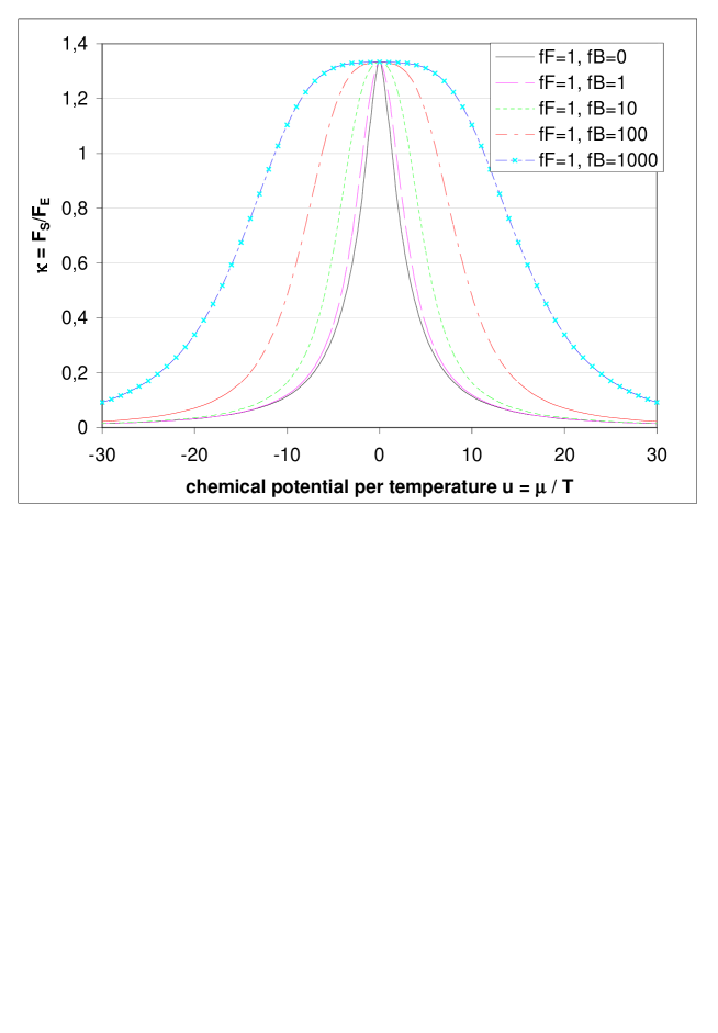
Figure 1: $\kappa=F_{S}/F_{E}$ as a function of the chemical potential per temperature of the fermions $u$, plotted for various values of the ratio of bosonic to fermionic degrees of freedom $r_{f}=f_{B}/f_{F}$

In order to get a better feeling of the functional relation between $u$, $r_{f}$ and $\kappa$ it is instructive to plot $\kappa(u,r_{f})$ as a function of the (fermionic) chemical potential per temperature $u$ for various - fixed - ratios $r_{f}=f_{B}/f_{F}$. Figure 1 shows such a plot. $\kappa(u)$ is a strictly positive, symmetric function of $u$ with a bell-shaped form, similar to a Lorentz-profile. $\kappa(u)$ attains its maximum value at $u=0$ and approaches zero quite rapidly for large absolute values of $|u|$. The maximum value $\kappa(0)=4/3$ is independent of the parameter $r_{f}$, whereas the width of the bell-shaped curve grows monotonically with $r_{f}$.

If $\kappa>4/3$ there is no solution for $u$ in the equation $\kappa(u,r_{f})=const$, whatever the ratio of the number of degrees of bosonic to fermionic degrees of freedom might be. Negative values of $\kappa$ are not possible either. $\kappa=0$ requires $u=\infty$, which doesn’t seem to make sense from a physical perspective. It is already clear from equation (16) that $\kappa$ must be a positive quantity for any reasonable closed thermodynamic system: $\kappa=ST/E$ can only become negative if either the entropy, the temperature or the total energy becomes negative. The microscopic statistical entropy is always non-negative, negative temperatures only arise for certain sub-systems and the total energy of a system is always positive (at least in general relativity). $\kappa=0$ requires either zero temperature or entropy or infinite energy, which is not physically sensible.

In the range $0<\kappa<4/3$ the chemical potential per temperature is always non-zero, and depends on the ratio $r_{f}$. For any given $r_{f}$ and $\kappa$ the corresponding value for $u$ can be read off from Figure 1 by determining the intersection of the horizonal line $\kappa=const$ with the bell-shaped curve parameterized by $r_{f}$. The innermost curve with $r_{f}=0$ describes a gas consisting exclusively out of fermions. Curves with larger $r_{f}$ lie above curves with lower $r_{f}$. All curves have one point in common: The global maximum at $u=0$ with $\kappa=4/3$. From this construction it is clear that for any given $0<\kappa<4/3$ the chemical potential per temperature $u$ attains its minimum value for the innermost curve parameterized by $r_{f}=0$ and that $u$ increases monotonically with $r_{f}$ (for fixed $\kappa$).

2.5.5 A closed formula for the chemical potential per temperature of the fermions $u$

Figure 1 allows a graphical determination of $u$. In general one has to solve equation (47). This relation can be expressed in the following form, which allows an experimental determination of $u$, whenever the ratios of fermionic to bosonic number- and energy-densities is known.

$$u=(\frac{4}{3}-\kappa)\frac{\pi^{4}}{30\zeta(3)}\frac{w_{E}+\overline{w_{E}}+2r_{f}}{w_{N}-\overline{w_{N}}}=(\frac{4}{3}-\kappa)\frac{\pi^{4}}{30\zeta(3)}\frac{\frac{e_{F}}{e_{B}}+1}{\frac{\Delta n_{F}}{n_{B}}}$$ (51)

where we have used

$$\frac{w_{N}-\overline{w_{N}}}{2r_{f}}=\frac{\Delta N_{F}}{N_{B}}=\frac{\Delta n_{F}}{n_{B}}$$ (52)

and

$$\frac{w_{E}+\overline{w_{E}}}{2r_{f}}=\frac{E_{F}}{E_{B}}=\frac{e_{F}}{e_{B}}$$ (53)

Note that $n_{B}$ is the (total) number-density of the bosons (all bosons added up, with no distinction between bosons and ”anti-bosons”), whereas $\Delta n_{F}$ denotes the fermion number density (number of fermions minus anti-fermions). $e_{B}$ and $e_{F}$ denote the total energy-densities of bosons and fermions.

Using equation (42) one can express equation (51) only in terms of the ratio $e_{F}/e_{B}$:

$$\frac{u^{2}}{\pi^{2}}(1+\frac{u^{2}}{\pi^{2}})=(\frac{4}{3}-\kappa)\frac{2r_{f}}{5}\left(\frac{e_{F}}{e_{B}}+1\right)$$ (54)

This is a quadratic equation in $u^{2}/\pi^{2}$, which is easy to solve whenever $r_{f}$, $\kappa$ and the ratio of the energy-densities of fermions to bosons is known.

Inserting equation (44) into equation (54) and using equation (53) we get a closed formula for $u$ in terms of the relevant parameters $\kappa$ and $r_{f}$:

$$u=\pi\sqrt{\frac{2}{3\kappa}\left(1+\sqrt{1+\frac{6}{5}\kappa(\frac{4}{3}-\kappa)(r_{f}-1)}\right)-1}$$ (55)

For $\kappa=4/3$ we find $u=0$, independent of $r_{f}$. Whenever $u$ is small we can derive an approximation formula from equation (55) or equation (54) for small $u$:

$$u\approx\pi\sqrt{(\frac{4}{3}-\kappa)(r_{f}+\frac{7}{8})\frac{2}{5}}$$ (56)

2.5.6 Supersymmetry

In the important supersymmetric case $r_{f}=1$, i.e. equal number of fermionic and bosonic degrees of freedom, equation (55) is very much simplified:

$$u=\pi\sqrt{\frac{\frac{4}{3}-\kappa}{\kappa}}$$ (57)

For $\kappa=1$ we find

$$u=\frac{\pi}{\sqrt{3}}$$

so that

$$\frac{e_{F}}{e_{B}}=\frac{w_{E}+\overline{w_{E}}}{2}=\frac{7}{3}$$

The ratio of the entropy-densities of fermions to bosons turns out to be simple, as well:

$$\frac{s_{F}}{s_{B}}=\frac{w_{N}\sigma_{F}+\overline{w_{N}\sigma_{F}}}{2\sigma_{B}}=\frac{3}{2}$$

For $\kappa=2/3$ we find ($r_{f}=1$)

$$u=\pi$$

so that

$$\frac{e_{F}}{e_{B}}=\frac{w_{E}+\overline{w_{E}}}{2}=\frac{13}{2}$$

and

$$\frac{s_{F}}{s_{B}}=\frac{w_{N}\sigma_{F}+\overline{w_{N}\sigma_{F}}}{2\sigma_{B}}=\frac{11}{4}$$

and

$$\frac{\Delta n_{F}}{n_{B}}=\frac{w_{N}-\overline{w_{N}}}{2}=\frac{\pi^{3}}{6\zeta(3)}\simeq 4.299$$

2.5.7 Some more relations

Generally it can be shown, that the ratio of the energy-, entropy-and number-densities are related by

$$\frac{s_{F}}{s_{B}}+1=\frac{3\kappa}{4}\left(\frac{e_{F}}{e_{B}}+1\right)$$ (58)

and

$$\frac{\Delta n_{F}}{n_{B}}=(\frac{4}{3}-\kappa)\frac{\pi^{4}}{30u\zeta(3)}\left(\frac{e_{F}}{e_{B}}+1\right)$$ (59)

From equation (58) one can see, that for $\kappa=4/3$ the ratios of the entropy-densities is equal to the ratio of the energy-densities. This reflects the well known result for an ultra-relativistic gas with zero chemical potential, where $s_{F}/s_{B}=e_{F}/e_{B}=7/8$.

An important quantity is the ratio of the energy-density of a fermionic particle anti-particle pair to a bosonic particle pair:

$$\frac{w_{E}+\overline{w_{E}}}{2}=\frac{5\omega^{2}}{6\kappa^{2}}-1$$ (60)

with

$$\omega(\kappa,r_{f})=1+\sqrt{1-\frac{6}{5}\kappa(\frac{4}{3}-\kappa)(r_{f}-1)}$$ (61)

For the supersymmetric case ($r_{f}=1$) the above defined quantity $\omega$ does not depend on $\kappa$. We have $\omega=2$, so that the ratio of the energy-densities reduces to

$$\frac{w_{E}+\overline{w_{E}}}{2}=\frac{10}{3\kappa^{2}}-1$$ (62)

The ratio of the number-density of a fermionic particle anti-particle pair (number of fermions minus anti-fermions) to a boson pair is given by:

$$\frac{w_{N}-\overline{w_{N}}}{2}=\frac{\pi^{3}}{18\zeta(3)}\frac{\omega}{\kappa}\sqrt{\frac{2\omega}{3\kappa}-1}=u\frac{\pi^{2}}{18\zeta(3)}\frac{\omega}{\kappa}$$ (63)

where we have used:

$$u=\pi\sqrt{\frac{2\omega}{3\kappa}-1}$$ (64)

In the supersymmetric case the ratio of the number densities reduces to

$$\frac{w_{N}-\overline{w_{N}}}{2}=\frac{\pi^{3}}{9\zeta(3)}\frac{1}{\kappa}\sqrt{\frac{4}{3\kappa}-1}=\frac{\pi^{2}}{9\zeta(3)}\frac{u}{\kappa}$$ (65)

2.6 The free energy

Knowing the grand canonical potential the free energy $F(T,V,N)$ can be calculated:

$$F=J+\sum{\mu N}=J+\mu_{F}N_{F}+\overline{\mu_{F}}\overline{N_{F}}=-\frac{F_{E}}{3}VT^{4}+uT\Delta N_{F}$$ (66)

or somewhat differently, using equations (38) and (40):

$$F=\left(u[F_{N}]-\frac{F_{E}}{3}\right)VT^{4}=(F_{E}-F_{S})VT^{4}=E-ST$$ (67)

The boson number $N_{B}$ does not show up in equations (66) and (67) and the fermion number appears as difference of the number of fermions minus anti-fermions. This reflects the fact that the chemical potential of any ultra-relativistic boson must be zero, whereas fermions are expected to have a non-zero chemical potential.

In the canonical formalism the entropy is calculated from the free energy by a partial differentiation with respect to $T$. In order to do this, the free energy must be expressed as a function of $T$, $V$ and the number of different particles $N_{i}$. This is not the case with equation (67).

2.6.1 A conservation law for the fermion number

From equation (66) one can show that the fermion number, i.e. the difference of fermion and anti-fermion numbers $\Delta N_{F}=N_{F}-\overline{N_{F}}$, is a ”conserved quantity” whenever $u$ (or rather $\mu_{F}$) takes on a non-zero value. If we take the partial derivative of $F$ with respect to $T$ we get

$$S=-\frac{\partial F}{\partial T}=\frac{4}{3}F_{E}T^{3}V+\frac{1}{3}\frac{\partial F_{E}}{\partial T}T^{4}V-\Delta N_{F}(u+T\frac{\partial u}{\partial T})-uT\frac{\partial\Delta N_{F}}{\partial T}$$

$$=\frac{4}{3}F_{E}T^{3}V-\Delta N_{F}u+T\left(T^{3}V[F_{N}]-\Delta N_{F}\right)\frac{\partial u}{\partial T}-uT\frac{\partial\Delta N_{F}}{\partial T}$$

$$=\left(\frac{4}{3}F_{E}-u[F_{N}]\right)T^{3}V-uT\frac{\partial\Delta N_{F}}{\partial T}$$ (68)

where we have used

$$\frac{\partial F_{E}}{\partial T}=3[F_{N}]\frac{\partial u}{\partial T}$$ (69)

and

$$\Delta N_{F}=[F_{N}]VT^{3}$$ (70)

By comparing the result of equation (68) with equation (40) one can see, that the entropy calculated from the free energy $F$ and the entropy derived from $J$ ($S=F_{S}VT^{3}$) are only equal if

$$uT\frac{\partial\Delta N_{F}}{\partial T}=\mu\frac{\partial\Delta N_{F}}{\partial T}=0$$ (71)

This means that the total fermion number $\Delta N_{F}$ (=number of fermions, counting fermions with a plus-sign and anti-fermions with a minus-sign) must be independent of temperature, whenever the chemical potential $\mu$ of the fermions is non-zero. It is quite remarkable, that the assumption of non-zero chemical potential gives us a thermodynamic ”conservation-law” for the total fermion number. At ultra-high temperatures there will be several different fermionic species present, which will undergo various particle-interchanging reactions. Yet the total fermion number, i.e. the difference of fermions and anti-fermions is conserved. Although the conservation of fermion number is built into the Standard Model of particle physics (all of the fundamental particles - excluding the gauge-bosons - are fermions and can only be created in pairs), the Standard Model does not really explain lepton or baryon number conservation. There is no dynamical symmetry associated with the merely empirical conservation of lepton ($L$) or baryon ($B$) number. Certain supersymmetric theories only conserve $L-B$. In this respect it comes somewhat of a surprise that there might be a thermodynamic origin to the conservation of fermion number. This hints to some deeper connection between thermodynamics, general relativity and quantum field theory. Note also, that the thermodynamic equations derived in the previous sections refer to the number-densities of a boson particle anti-particle pair in a symmetrized version ($N_{B}+\overline{N_{B}}$ with $N_{B}=\overline{N_{B}}$), whereas the fermion anti-fermion number-densities always appear as anti-symmetrized quantities $\Delta N_{F}=N_{F}-\overline{N_{F}}$.

The fermion number ”conservation law” can only be applied to fermions, because - as discussed beforehand - only fermions can have a non-zero chemical potential. For relativistic bosons the chemical potential must be zero, therefore equation (71) does not include the boson number $N_{B}$.. This result is not quite unexpected: A conservation law for boson-numbers would be in conflict with the fundamental physical principle of gauge-invariance: All fundamental bosons are gauge-bosons, i.e. they mediate the electro-magnetic, weak and strong interactions between the (fermionic) particles of the Standard Model. It is mandatory for a gauge boson that it can be created (in a virtual process) without being restrained by a particle-number conservation law.

2.7 Zero chemical potential - a rather special case

In this section I will discuss the rather special subcase of a zero chemical potential of the fermions. We will see that a zero chemical potential arises only under very special conditions.

The relevant thermodynamic quantities $F_{S}$ and $F_{E}$, which appear in the relations for the energy- and entropy-densities of an ultra-relativistic gas, only depend on $u$ and the number of fermionic and bosonic degrees of freedom. At ultra-high temperatures, above the unification scale, one expects that the number of fundamental degrees of freedom does not change and that the chemical potential per temperature remains constant. Therefore it seems attractive to assume that $F_{E}$ and $F_{S}$ are independent of temperature $T$. If this is actually the case, calculating the entropy from the free energy via equation (67) is trivial.

In this rather special case one gets an independent expression for the entropy, which - combined with equation (12) - allows one to derive a relation between $F_{E}$ and $F_{S}$. This relation fixes $\kappa$, so that we can determine $u$ whenever the number of degrees of freedom $f_{F}$ and $f_{B}$ of the ultra-relativistic gas is known.

There is no guarantee that $F_{E}$ and $F_{S}$, which depend on $f_{F}$, $f_{B}$ and $u$ are independent of the thermodynamic variable $T$, though. Even at ultra-high temperatures we cannot be sure that the chemical potential per temperature $u$ of the fermions does not depend on $T$. The number of ultra-relativistic fermionic and bosonic degrees of freedom change whenever the temperature reaches the mass-threshold of a particular species. This induces an indirect dependence of $F_{E}$ and $F_{S}$ on temperature, which most likely has an - indirect - effect on the value of $u$. Note also, that the assumption of scale invariance at high temperatures not necessarily requires $\mu\propto T$. A logarithmic dependence is compatible with scale invariance as well. One therefore must check very carefully if the results based on the assumption of ”constant” $F_{E}$ and $F_{S}$ are consistent. In fact, equation (69) already tells us, that constant $F_{E}$ and $F_{S}$ requires that $\partial u/\partial T=0$ or $u=0$.

Assuming that $F_{E}$ and $F_{S}$ do not depend on $T$, one gets the following alternative expression for the entropy:

$$-S=\frac{\partial F}{\partial T}=4(F_{E}-F_{S})VT^{3}$$ (72)

If we compare the above value for the entropy with the entropy derived from the grand canonical potential, given by equation (12), we can determine $\kappa$. We find $\kappa=4/3$.

$\kappa$ has been expressed as a quadratic function of $u^{2}$ and $r_{f}$ in equation (47). A close look at this equation shows (see also Figure 1), that whatever the value of $r_{f}$ might be, the only solution for $\kappa=4/3$ is $u=0$. Whenever an ultra-relativistic gas of fermions and bosons can be described by $\kappa=4/3$ the chemical potential of the ultra-relativistic fermions must be identical zero. This could already have been seen from equation (40).

The assumption that the chemical potential of the fermions should be zero at high temperatures is not new. An argument for a nearly zero chemical potential at high temperatures in a cosmological context can be found in Weinberg’s classical treatise [15, p. 531]. Weinberg’s argument is based on the assumption, that the number of photons in the universe at these high temperatures is vastly larger than the number of baryons, i.e. by a factor $10^{9}$.

The result $u=0$ is self-consistent. For $u=0$ the partial derivative of $F_{E}$ and $F_{S}$ with respect to $T$ is zero, trivially. Note also, that for $u=0$ the particle numbers $N_{i}$ of the different species need not be considered in the expression for the free energy (the chemical potentials of all particles are zero and the $N_{i}$ are always multiplied by the chemical potentials $\mu_{i}$ in the expression for the free energy). In the particular case of an ultra-relativistic gas with zero chemical potential the free energy $F$ is equal to the grand canonical potential $J$, so that it is not surprising that it doesn’t matter whether we derive $S$ by a partial integration from $J=-(F_{E}/3)\,VT^{4}$ or from $F=(F_{E}-F_{S})\,VT^{4}$, assuming that $F_{E}$ and $F_{S}$ are constant.

The combination $u=0,\kappa=4/3$ therefore is a perfectly possible choice of parameters for an ultra-relativistic gas. Furthermore, this choice minimizes the free energy to its least possible value: $F=-E/3$. Why then consider the more general case $\kappa<4/3$ and $u\neq 0$, where the free energy is higher?

It is not possible to give a short answer just right now. Exterior constraints might impose a different value of $\kappa$ on the whole system. We will see in the next section that self gravitating systems are characterized by values of $\kappa$ which lie in the range $0<\kappa\leq 1$. Although gravity is a weak force, it has the virtue of being positive all the time. For sufficiently large systems it will be quite difficult to escape the exterior constraints imposed on a thermodynamic system by the general theory of relativity.

3 On the relation between entropy, energy and free energy for self gravitating systems

The purpose of this section is to shed some light on the physical interpretation of the thermodynamic parameter $\kappa$, which turned out to be of some relevance in the previous section. We will see that whenever the entropy of a closed system can be expressed as a function of the total energy alone, i.e. $S=S(E)$ (and when $\kappa\approx const$) the entropy $S$ and the total energy $E$ are related by a power-law. $\kappa$ then is nothing else than the exponent in the relation between $S$ and $E$. Some examples for physical systems which can be described by such a power relation are given at the end of this section.

3.1 A linear relation between the total and the free energy

Equation (15) implies the following relation between the free energy $F$ and the total energy $E$.

$$F=E-ST=(1-\kappa)E$$ (73)

We find, that $F$ and $E$ are proportional to each other, with the factor of proportionality given by $1-\kappa$. Note that the above equation doesn’t necessarily imply a strictly linear relation. Equation (15) is completely general, as long as no assumptions with respect to $\kappa$ are imposed. One can regard the above equation as a definition for $\kappa$.

At ultra-relativistic temperatures we have seen that the allowed range for $\kappa$ is quite restricted: $0<\kappa\leq 4/3$. It is clear that $\kappa$ can only vary very moderately within a particular thermodynamic model, at least at high temperatures. Here we are not interested in the most general thermodynamic model possible, but rather in the cases which are relevant from a physical perspective. As has been already discussed in the previous section, at ultra-high temperatures one expects $u$ to be nearly constant: Due to the lack of a specific mass- or energy scale at ultra-high temperatures the chemical potential of an ultra-relativistic fermion will depend nearly linearly on the temperature. As $\kappa$ is a function of $u$ and $r_{f}$ only, it must be nearly constant whenever the ratio of bosonic to fermionic degrees of freedom $r_{f}$ does not change and the chemical potential of the ultra-relativistic fermions has the expected nearly linear temperature-dependence.

From equation (73) one sees, that any thermodynamic system with constant $\kappa$ is characterized by the property, that it’s free energy $F$ is exactly proportional to the total energy $E$. The value $\kappa=1$ is special. It renders the free energy exactly zero, regardless of the total energy of the system.

Another interesting value for $\kappa$ was pointed out in the previous section: For $\kappa=4/3$ the chemical potential of all particles zero, regardless of the number of degrees of freedom of fermions and bosons. In this case we attain the well-known result, that the free energy $F$ of an ultra-relativistic gas (with zero chemical potential) is equal to the grand-canonical potential $J$. However, the free energy is negative with $F=J=-E/3$.

Are there other values of $\kappa$ which might be of relevance and are there actually systems - in theory and in praxis - that can be described by a specific value of $\kappa\neq 4/3$?

3.2 Thermodynamic systems with S = S(E)

Before I attempt to answer this question, it is instructive to find out what more can be inferred about the thermodynamic properties of a closed system with nearly constant $\kappa$. In order to make specific predictions some additional assumptions are required. We are interested in the thermodynamic behavior of a gas at ultra-high temperatures, i.e. temperatures well above the electron mass threshold. Such extreme temperatures are only conceivable for self-gravitating systems, such as in the early phase of the universe or during relativistic collapse of a massive star. For sufficiently compact gravitationally bound objects, such as neutron stars (and even more so for black holes) there is a more or less rigid relationship between size (= boundary area) and the total energy (=asymptotic gravitating mass) of the system. It appears as if this is a universal property of bounded self gravitating systems, whose internal energy sources - such as thermo-nuclear reactions - have ceased so that their energy output is determined by gravitational phenomena alone.

Whenever there is a definite relationship between the system’s spatial extension and its total energy, i.e. $V=V(E)$ - or alternatively $A=A(E)$, where $A=\partial V$ is the system’s boundary area - the temperature can only depend on $E$. This follows from the ultra-relativistic gas law $E\propto V(E)T^{4}$ and the assumption of scale-invariance at ultra-high temperatures. In this case the entropy will also be an exclusive function of $E$, as $S\propto VT^{3}$ at ultra-relativistic temperatures. The result is, that whenever the temperature of a system is high enough and it’s spatial extension depends only on its total energy, the system’s entropy can be expressed as a function of $E$ alone:

$$S=S(E)$$

This is even true for the most extreme version of a self-gravitating system, a black hole: Although the ”volume” of a black hole cannot be properly defined and it’s interior matter state clearly is not that of an ultra-relativistic gas, it’s boundary area $A$ remains a meaningful concept. For a spherically symmetric black hole we find $S\propto A\propto E^{2}$. In the more general case of a Kerr-Newman black hole the entropy also depends on the exterior conserved quantities, which are the black hole’s angular momentum $J$ and charge $Q$. However, this additional complication does not change the results that will be obtained in this and the following sections. The essential requirement is that the total differential of the entropy only depends on one of the three variables $E,V,N$, i.e. $dS=(\partial S/\partial E)dE$ + terms independent of $V$ and $N$. This requirement is fulfilled by all classical black hole solutions.

Whenever the entropy $S$ happens to be a function of the energy $E$ alone, one can use the well known thermodynamic identity:

$$\frac{\partial S}{\partial E}T=1$$ (74)

and replace the partial derivative with a total derivative. This allows one to express the temperature as the total derivative of $E$ with respect to $S$:

$$T=\frac{dE}{dS}$$

Inserting this into equation (15) we get:

$$\frac{dE}{E}=\kappa\frac{dS}{S}$$ (75)

This equation can be integrated, whenever $\kappa$ is a function of energy (or entropy) alone. If $\kappa$ is constant, the integral is trivial:

$$S=\alpha\cdot E^{\frac{1}{\kappa}}$$ (76)

$\alpha$ is an integration constant. We find, that whenever the entropy of a closed system is related to its total energy by a power-law, $\kappa$ is nothing else than the exponent describing this relation, i.e. $E\propto S^{\kappa}$. The temperature follows from equation (74):

$$T=\frac{\kappa}{\alpha}E^{1-\frac{1}{\kappa}}$$ (77)

It is important to keep in mind, that the relation between total energy and total entropy is a global one, which is only valid for the system as a whole. The temperature derived in equation (77) thus must be interpreted as the ”global” temperature of the system in question. A global relation between entropy and energy does not necessarily mean, that one can define a local temperature at every space-time point.

All this has been quite abstract. The question that naturally arises at this point is, whether we actually can find (closed) systems in nature that are characterized by a power-law dependence between $E$ and $S$, or more generally by a relation $S=S(E)$. It appears, that $S=S(E)$ is a common occurrence among self-gravitating systems.

3.3 Black hole solutions

Let us first apply equations (76, 77) to the simplest theoretical self gravitating system known, a spherically symmetric black hole. For the Schwarzschild black hole we have the (global) relation $S=4\pi E^{2}/\hbar$, where $E$ is taken to be the gravitational mass of the black hole measured at spatial infinity. We find $\kappa=1/2$ and $\alpha=4\pi/\hbar$. Inserting these values into equation (77) then gives us - not unexpectedly - the right relation for the Hawking temperature of a black hole, measured at spatial infinity, i.e. $T=\hbar/(8\pi E)$.

According to the relation $F=(1-\kappa)E$, the free energy for a spherically symmetric black hole amounts to half it’s total energy. We will see later, that there are exact solutions to the classical field equations, which minimize $F$ to zero in the interior, matter-filled region. In a certain sense one can say, that a classical black hole does a good job in minimizing the free energy globally ($F=E/2$), but fails to minimize the free energy locally to the least possible value conceivable for a self-gravitating system ($F=0$).

The relation $S=S(E)$ can be extended to charged and rotating black holes. Although the relation between the total energy and entropy of the more general black hole solutions also depends on the total charge(s) $Q_{i}$ and the total angular momentum $J$, these quantities are globally conserved. The total differential of the entropy $dS$ only depends on $dE$, $dQ_{i}$ and $dJ$, but not on $dV$ or $dN$. For an isolated black hole in an exterior vacuum space-time the conserved quantities cannot change, so that $dJ=dQ_{i}=0$. Whenever we can consider the black hole and its surroundings as a closed system, we should not treat the exterior conserved quantities as independent thermodynamic variables, so that the temperature can be derived from a total derivative $T=\partial E/\partial S=dE/dS$ whenever $dJ=dQ_{i}=0$.

This can be seen as follows: For a Kerr-Newmann black hole $\kappa$ can be calculated from its definition in equation (16). Using the well known relations for the mass $M=E$, entropy $S$ and temperature $T$ of a Kerr-Newman black hole we find:

$$\kappa=\frac{ST}{E}=\frac{1}{2}\sqrt{1-\left(\frac{Q}{M}\right)^{2}-\left(\frac{J}{M^{2}}\right)^{2}}$$ (78)

or alternatively, as a function of $J,Q$ and area $A$:

$$\kappa=\frac{1}{2}\frac{1-\left(\frac{4\pi Q^{2}}{A}\right)^{2}-\left(\frac{8\pi J}{A}\right)^{2}}{\left(1+\frac{4\pi Q^{2}}{A}\right)^{2}+\left(\frac{8\pi J}{A}\right)^{2}}$$ (79)

$\kappa$ lies in the range $0\leq\kappa\leq 1/2$ and only depends on the dimensionless ratios $Q/M$ and $J/M^{2}$ (alternatively on $Q^{2}/A$ and $J/A$). For an extreme Kerr-Newman black hole $\kappa=0$. In this case the black hole’s free energy is equal to its total energy. This is the maximum possible value for the free energy. For a general Kerr-Newman black hole of given mass $M$ or area $A$ the free energy $F=(1-\kappa)E$ is minimized, when $\kappa$ takes on its maximum value. This is the case for $\kappa=1/2$, corresponding to $Q=J=0$, i.e. a spherically symmetric Schwarzschild black hole. The expectation, that the Schwarzschild black hole should be the thermodynamically preferred state, which minimizes the free energy, is quite in agreement with the general expectation, that any charged or rotating black hole will shed angular momentum and charge, until it becomes a spherically symmetric Schwarzschild black hole. A very important parameter for the more general black hole solutions is the irreducible mass, which is proportional to the black hole’s horizon area / entropy. Whereas the mass $M$ of a black hole can change in the various allowed processes which extract energy (but not entropy) from a black hole, a black hole’s mass can never be lowered below its irreducible mass by any classical process. For a Schwarzschild black hole its irreducible mass is identical to its gravitating mass, so - from the classical viewpoint - a further reduction of the total energy is not possible.

It is possible to determine the correct relation between entropy and total energy of a Kerr-Newman black hole through $\kappa$, assuming that the partial derivative $1/T=\partial S/\partial E$ can be replaced by a total derivative:

$$\kappa=\frac{ST}{E}=\frac{S}{E}\frac{\partial E}{\partial S}=\frac{S}{E}\frac{dE}{dS}$$

This is a differential relation between $S$ and $E$, which can be integrated:

$$\frac{dS}{S}=\frac{dE}{\kappa E}=\frac{2dE}{E\sqrt{1-\left(\frac{Q}{E}\right)^{2}-\left(\frac{J}{E^{2}}\right)^{2}}}$$

This integration is easy to perform by a change of variables $x=E^{2}$:

$$\ln{S}=\int{\frac{dx}{\sqrt{x^{2}-Q^{2}x-J^{2}}}}=\ln{(2\sqrt{x^{2}-Q^{2}x-J^{2}}+2x-Q^{2})}+C$$ (80)

Exponentiating the above result and replacing $x$ with $E^{2}=M^{2}$ gives us the following relation:

$$S\propto 2M^{2}+2\sqrt{M^{2}-Q^{2}-\frac{J^{2}}{M^{2}}}-Q^{2}$$ (81)

This is the correct formula for the entropy of a Kerr-Newman black hole, if we multiply the right hand side by $\pi/\hbar$.

Note that the quadratic correspondence between energy and entropy $S\propto E^{2}$ holds approximately for charged and rotating black holes. For instance, an extreme Kerr black hole with $M^{2}=J$ and $Q=0$ has $S=2\pi J/\hbar=2\pi M^{2}/\hbar$. For an extremely charged Reissner Nordström black hole with $J=0$ and $Q=M$ we find $S=\pi Q^{2}/\hbar=\pi M^{2}/\hbar$.

3.4 The holographic solution

Classical black holes are vacuum solutions of the field equations and therefore not very well suited for a thermodynamic analysis based on microscopic statistical thermodynamics, which requires matter. Are there other systems to which equations (76, 77) apply?

Recently the so called holographic solution was discovered in [10]. The holographic solution is an exact solution of the original Einstein field equations. It describes a self-gravitating system of arbitrary size with an interior string equation of state. The holostar has properties very similar to a black hole. Most notably its entropy and temperature at infinity are proportional to the Hawking result, as can be shown by simple microscopic statistical thermodynamic analysis of the interior matter-filled space-time. The holographic solution and its properties are discussed extensively in [11, 12, 9, 13]. Here I will just point out some of the results which are relevant in the context of this paper.

For any thermodynamic system the total energy $E$ is one of its key variables. In contrast to the entropy, which is a pure number, and the temperature, which is a local parameter, whose normalization is tied to the total energy, the concept of total energy is somewhat ambiguous in a curved space-time. In general relativity it is of paramount importance to define the point of reference, from which the total energy of the space-time is calculated. In the black hole case the only sensible reference ”point” is the position of an asymptotic observer at spatial infinity. The temperature and energy attributed to a black hole refer to this point of reference. In contrast to a black hole the holostar solution is regular throughout the whole space-time. There is no event-horizon which separates two causally disconnected regions. Therefore other choices of reference-point are possible.

If we take spatial infinity as reference point, we get $\kappa=1/2$, equal to the black hole case. This is not unexpected, because a holostar viewed from the exterior space-time is practically indistinguishable from a black hole.

However, another natural reference point is the position of the holostar’s spherical boundary membrane. The effective potential for the geodesic motion of particles has a global minimum at this position, so that the membrane might be viewed as a ”better” reference position for a stationary observer. If one calculates the total energy with respect to this reference point (by a proper integral over the interior energy-density) one gets $E\propto r_{h}^{3/2}$, where $r_{h}$ is the radial coordinate position of the holostar’s boundary. For large holostars $r_{h}$ is nearly identical to the holostar’s gravitational radius, so that $r_{h}\simeq 2M$. The entropy of the holostar is proportional to its boundary area, i.e. $S\propto r_{h}^{2}$. Therefore the holostar is characterized by $S\propto E^{4/3}$, if the total energy is evaluated at the boundary membrane. This dependence translates to $\kappa=3/4$, which predicts $T\propto E^{-1/3}\propto r_{h}^{-1/2}$, which is the correct temperature dependence for the holostar’s surface temperature at the boundary membrane. Using the exact numerical figures from [11] (and setting $\hbar=1$) one finds $\alpha=\pi\,3^{4/3}r_{0}^{2/3}$, from which $T=1/(4\pi\sqrt{r_{0}r})$ follows, exactly the result derived in [11] and independently in [12]. $r_{0}$ is a (constant) scale factor with dimensions of length, roughly equal to twice the Planck length.

A third natural reference point is that of a geodesically moving observer in the interior space-time. Note, that this is a local point of reference, as the observer moves - in highly relativistic motion - through the interior space-time. But the local observer sees only a small fraction of the whole space-time: He can never look beyond his current Hubble-radius. One cannot expect that the global relations are applicable to this local observer. If we restrict the calculation of ”total” entropy and energy to the local Hubble-volume of the co-moving observer, we get $E\propto r$ and $S\propto r^{3/2}$, where $r$ is the current value of the scale factor ($H\propto 1/r$). This translates to $\kappa=2/3$, which predicts a temperature dependence $T\propto 1/\sqrt{E}\propto 1/\sqrt{r}$, again exactly the temperature dependence that the co-moving observer experiences in his local Minkowski frame.

Quite interestingly, the local thermodynamic properties of the interior holostar space-time can also be characterized by a different constant value of $\kappa$, which is tied to the viewpoint of a - most likely hypothetic - stationary observer at constant radial coordinate position $r$. In [12] it has been shown, that the holostar’s total entropy and its temperature at infinity are exactly proportional to the Hawking result if one calculates the local entropy-density and temperature in the ($t,r,\theta,\varphi$) coordinate-system, where the holostar space-time appears static. However, unless $\kappa=1$ the holostar’s temperature at infinity $T_{\infty}$ and its total entropy $S$ are not related with the right factor. If the holostar-solution is to reproduce the Hawking-result with the correct relation between $T$ and $S$, $\kappa$ must be unity in the interior space-time. This result is quite remarkable, as $\kappa=1$ implies that the free energy $F$ be identical zero. Therefore the holostar minimizes it’s interior free energy to zero, at least from the viewpoint of a stationary interior observer.

3.5 Friedmann-Robertson-Walker type solutions

Does the relation $S\propto E^{1/\kappa}$ hold in other contexts? There is another self-gravitating system, which we are quite familiar with. It is called ”the universe”. Can the universe be described by a relation between $S$ and $E$ with $\kappa=const$?

In order to answer this question one has to analyze the evolution of energy- and entropy-densities in the universe’s different evolutional stages (matter-dominated, radiation-dominated, etc.). Quite clearly this analysis is model-dependent. In this section the analysis will be done in the context of the standard Friedmann Robertson-Walker (FRW) model for the universe, which is based on the so called cosmological principle. In the next section I will discuss a somewhat more exotic model of a flat, holographic universe.

In an homogeneously expanding space-time the expansion must be nearly adiabatic, as there can be no net heat flow into or out of a particular co-moving volume element in a homogeneous universe (unless one assumes extra dimensions). With this assumption entropy is approximately conserved in any co-moving volume. This means, that the entropy-density $s$ will always be proportional to the inverse volume. With the known relation $R\propto 1/T$ between the scale factor $R$ and the temperature $T$ we find $s\propto T^{3}$.

In the matter-dominated era the energy-density $e$ has the same behavior: $e\propto 1/R^{3}\propto T^{3}$ (unless we assume that particles are created or destroyed, violating local energy-conservation in a co-moving volume). Therefore $s\propto e$, which suggests $\kappa=1$. However, there is a slight difficulty in applying this finding to the framework developed so far. We have assumed a power-law between the total entropy and energy, which not necessarily translates to the same power-law for the densities. Determining the ”total entropy” or the ”total energy” of the universe is tricky, if not impossible. We would have to multiply the respective densities with the ”total volume of the universe” at a given time. This might not be well defined, particularly for an open universe, which cannot be ruled out by today’s measurements.

Yet there is an interesting observation: The product of the entropy-density (which scales with $T^{3}$) and the ”volume of the universe” (which scales with $R^{3}\propto 1/T^{3}$) is constant. The same applies to the product of the energy-density with the volume for the matter-dominated era. So we might still be able to relate the total (constant) entropy to the total (constant) energy of the universe, by calculating the (finite) ratio of the entropy to the energy in any finite co-moving region. This ratio is time- and position-independent for a matter-dominated FRW-universe. As the ratio is the same for any arbitrary finite region, it is reasonable to assume that $S\propto E$ for the whole universe, even if its total volume, energy and entropy may be infinite. Note also, that in a homogeneously expanding universe any one of its finite parts can be regarded as a closed system to a very good approximation, so that we can calculate the total energy and entropy for any large enough part without having to know what lies beyond. The relation found by this procedure will be valid for the whole universe, at least so far as the cosmological principle can be trusted.

With this somewhat debatable interpretation we find $\kappa=1$ for the matter-dominated era. However, in the matter-dominated era the particles are not relativistic, so the formula for an ultra-relativistic gas cannot be applied.

Yet when we look far back into the past where the universe is expected to be radiation-dominated, an ideal gas of ultra-relativistic fermions and bosons should be a very good approximation to the thermodynamics in the very early history of the universe. Can we attribute a sensible value to $\kappa$ in this case?

Assuming that the expansion remains adiabatic, we find that the energy density scales with $T^{4}$ and the entropy-density with $T^{3}$. This gives us $s\propto e^{3/4}$, which - naively - could be interpreted as $\kappa=4/3$. The problem is, that in the radiation dominated era the ”total energy” in any (finite) co-moving volume element diverges ($E\propto T$), whereas the ”total entropy” in the same volume remains constant. With respect to the total energy and entropy in a given co-moving volume element one would rather have to postulate $\kappa\propto\ln{T}\propto\ln{E}$, i.e. a non-constant value of $\kappa$ which depends logarithmically on the temperature. This construct is highly problematic. It requires a maximum temperature, because for unbounded temperatures the ceiling $\kappa\leq 4/3$ would be exceeded. Furthermore, the entropy cannot be a function exclusively of the total energy. This would require $\kappa$ to be a function of total energy alone, i.e. $\kappa=c\ln{E}$. But the ”constant” of proportionality $c$ depends on the particular choice of the co-moving volume. Unless there is a ”preferred” volume element, such as the total volume of a closed universe, the choice of the correct co-moving volume is ambiguous.

3.6 Holographic homogeneous flat universes

An interesting case is that of a homogeneously expanding flat ($\Omega=1$) universe with the additional assumption, that the matter in this universe strictly obeys the holographic principle. This means that the entropy in any space-time region doesn’t scale with volume, but with the area of it’s boundary. If we denote the co-moving length by $r$, we find the following dependence for the entropy in a holographic flat universe:

$$S\propto r^{2}\propto A\propto V^{\frac{2}{3}}$$ (82)

For the total matter in a holographic universe let us assume an equation of state of the following general form:

$$P=w\frac{E}{V}$$ (83)

In the radiation-dominated era we have $w=1/3$, in the matter-dominated era $w=0$. A vacuum-dominated era is characterized by $w=-1$, a string-dominated era by $w=-1/3$ and a domain-wall dominated era by $w=-2/3$.

Note that $w\neq 1/3$ is not necessarily in contradiction with the equation of state for an ultra-relativistic gas. With $w$ we denote the equation of state for all types of matter/energy in the universe. Although matter at ultra-high temperatures will almost certainly include a significant contribution of radiation, the matter must not necessarily consist exclusively out of radiation. If string theory is the correct description of the phenomena at the high energy limit, we should expect a significant ”string contribution” to the mass-energy at ultra-high temperatures. In this respect it is quite remarkable, that by combining a vacuum stress-energy tensor ${T_{\mu\nu}}\propto diag(1,-1,-1,-1)$ with the stress energy-tensor for radiation ${T_{\mu\nu}}\propto diag(1,1/3,1/3,1/3)$ one gets the stress-energy tensor of an isotropic string gas, whenever the radiation and vacuum contributions are equal:

$${T_{\mu\nu}}_{vac}+{T_{\mu\nu}}_{rad}\propto diag(1,-1/3,-1/3,-1/3)\propto{T_{\mu\nu}}_{string}$$ (84)

with

$$\rho_{vac}=\rho_{rad}=\frac{\rho_{string}}{2}$$

Therefore, a universe with an overall string equation of state can still contain a significant fraction of radiation, if the radiation is paired with an equivalent contribution of ”vacuum energy”.

If one knows the equation of state for the total matter state one can calculate the dependence of the total energy on the volume via the thermodynamic relation $dE=-PdV$, replacing $P$ with equation (83):

$$\frac{dE}{E}=-w\frac{dV}{V}$$ (85)

The above equation can be easily integrated, yielding

$$E\propto V^{-w}$$ (86)

Relating this to equation (82) we get the following correspondence between $S$ and $E$:

$$S\propto E^{-\frac{2}{3w}}$$ (87)

so that we can identify $\kappa$ with the equation of state parameter $w$:

$$\kappa\longleftrightarrow-\frac{3w}{2}$$ (88)

An interesting case is $w=-1/3$, which corresponds to a string equation of state. In this case $\kappa=\frac{1}{2}$, so that

$$E\propto V^{\frac{1}{3}}\propto\sqrt{A}\propto r$$ (89)

and

$$S\propto V^{\frac{2}{3}}\propto A\propto r^{2}$$ (90)

These relations are identical to the results for a spherically symmetric black hole, when the scale-factor $r$ is identified with the Schwarzschild radius. We arrive at the remarkable conclusion, that a holographic flat universe with a string equations of state for the total matter-content delivers the same dependence between total energy $E$, area $A$ and entropy $S$ as a spherically symmetric black hole. It is well known that the entropy and temperature for an extreme or nearly extreme black hole (including the correct grey-body factors) can be derived rigourously in the context of string theory by counting string / brane states in the low coupling limit. The construct of a holographic flat universe suggests another non-trivial connection between the properties of stringy matter, the holographic principle and black hole type objects, for which the relation $S\propto A$ holds.

In order to see how a flat holographic universe fits into the big bang picture of a a hot, high density initial state, one has to analyze the dependencies of energy-density and temperature on the scale factor $r$.

From equation (86) one finds that the energy-density scales as

$$e=\frac{E}{V}\propto V^{-(w+1)}\longleftrightarrow V^{-\frac{2}{3}(\frac{3}{2}-\kappa)}$$ (91)

The energy-density increases with decreasing scale-factor as long as $w>-1$. The limiting case $w=-1$ is the equation of state for a ”true” cosmological constant. $w>-1$ corresponds to the condition $\kappa<3/2$ via equation (88). This condition is always fulfilled for $\kappa$ in the permissible range $(0,4/3]$.

Using equation (87) the temperature in a flat holographic universe can be calculated:

$$T=\frac{dE}{dS}\propto V^{-(\frac{2}{3}+w)}\longleftrightarrow V^{\frac{2}{3}(\kappa-1)}$$ (92)

The temperature increases with decreasing scale factor whenever $w>-2/3$. The limiting case $w=-2/3$ is the equation of state of a domain wall. A flat holographic universe expanding from a hot, high density initial state therefore requires $w>-2/3$, or alternatively $\kappa<1$.

Equation (88) relates $\kappa$ to the equation of state parameter $w$. We have already seen that the implicit equation $\kappa(u,r)=const$ only gives solutions in the range $0<\kappa\leq 4/3$. But this requirement was derived in the context of microscopic statistical thermodynamics of an ultra-relativistic ideal gas, which has an equation of state with $w=1/3$. With the somewhat shaky assumption, that the formalism developed for an ultra-relativistic gas can be extended to other forms of matter, and that the permissible range for $\kappa=ST/E$ is more or less independent of the matter temperature, one can derive a restriction on the admissible $w$-values (for the total equation of state) in a flat holographic universe:

$$-\frac{8}{9}\leq w<0$$ (93)

It is intriguing to interpret this result such, that in a flat homogeneous holographic universe the only equation of state that make sense (for the total matter contribution) is $w=-1/3$ for stringy matter and $w=-2/3$ for matter composed out of domain-walls.

The above result relied on $0<\kappa\leq 4/3$. If one demands a hot initial state, the requirement $\kappa<1$ restrains $w$ somewhat further. We find $-2/3<w<0$, which seems to indicate that stringy matter is the only possible form of matter at ultra-high temperatures in a holographic flat universe. Note, that this does not necessarily imply that all of the matter at ultra-high temperatures must actually be strings.

4 Necessary conditions for a thermodynamical origin of a matter anti-matter asymmetry at ultra-high temperatures

The purpose of this section is to analyze from the most general point of view, what conditions have to be met that microscopic statistical thermodynamics could be a possible cause for a matter anti-matter asymmetry in a closed system at ultra-high temperatures.

It is not the purpose of this section to give arguments whether it is likely, unlikely, or impossible, if these conditions actually apply to a realistic self-gravitating object. This would be a futile task, anyway, because - as yet - we lack a universally accepted self-consistent description for a realistic self-gravitating object containing matter, to which microscopic statistical thermodynamics could be applied. The discussion of a possible application of the results derived in this section to some particular solutions of the field equations is referred to the last section.

However, in the previous section several examples of simple theoretical self-gravitating systems have been given, for which the entropy $S$ turned out to be an exclusive function of the total energy $E$ (and of exterior, conserved quantities, such as angular momentum and charge). Most of these systems were characterized by a power-law relating $S$ and $E$. Whenever this was the case, $\kappa$ could be identified as the exponent in the relation $E\propto S^{\kappa}$.

The assumption of a power-law dependence between $S$ and $E$ appears to be applicable to a wide range of self-gravitating systems, regardless of their size. This suggests the conjecture, that any self-gravitating system might be characterized by such a power-law, and that different realizations of self-gravitating systems can be classified by their specific value of $\kappa$.

Whenever $\kappa$ falls into the allowed range $0<\kappa\leq 4/3$, one can determine the chemical potential per temperature $u$ of the ultra-relativistic fermions, when the ratio $r_{f}$ of bosonic to fermionic degrees of freedom is known. The fermionic chemical potential is generally non-zero and proportional to the temperature, except for the rather special case $\kappa=4/3$.

A non-zero value of $u$ at ultra-high temperatures is very interesting with respect to the matter-antimatter asymmetry, which can be found in our universe today. A non-zero chemical potential naturally induces an asymmetry between fermions and anti-fermions. This can be seen in Figure 2, where the number- and energy-densities of a single fermionic degree of freedom is plotted as a function of $u$.

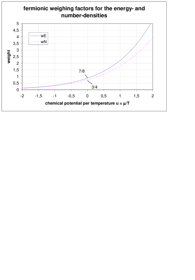
Figure 2: Fermionic weighting factors for the energy density $w_{E}$ and number-density $w_{N}$ as a function of the chemical potential per temperature $u$, normalized to energy- and number-densities of a single bosonic degree of freedom

As can be seen from Figure 2 both the number- and energy-densities of the fermion gas are monotonically increasing functions of $u$. With the convention that $u>0$ for fermions and $-u<0$ for anti-fermions one can easily see, that the number- and energy-densities of the ultra-relativistic fermions will always be larger than those of the anti-fermions for any non-zero value of $u$. The extent of the asymmetry depends on $u$. The higher $u$ gets, the larger the interval $[-u,u]$ separating fermions from anti-fermions becomes, with the result that the asymmetry increases. Except for very small values of $u$ the asymmetry is substantial. Let us denote the ratio of the fermionic energy-density to that of the anti-fermions by $\eta_{E}$:

$$\eta_{E}=\frac{w_{E}}{\overline{w_{E}}}=\frac{w_{E}(u)}{w_{E}(-u)}$$ (94)

When $u$ is of order unity, this ratio is already as high as $\eta_{E}\approx 7.3$. The ratio of the number-densities is somewhat lower, $\eta_{N}\approx 6.7$.

$\kappa$	$f_{B}/f_{F}$	$u$	$\sigma$	$\eta_{E}$	$\eta_{N}$
1.3	0	0.107512	4.19374	1.93178	1.87925
1.3	1/3	0.126313	4.01018	2.16376	2.09484
1.3	1	0.157276	3.85278	2.60340	2.50067
1.3	10	0.376545	3.63858	8.84216	8.03993
1.3	1000	2.740314	3.59779	20350.5	11335.5
1.2	0	0.736353	3.87561	4.05095	3.81702
1.2	1/3	0.856558	3.73527	5.08402	4.74221
1.2	1	1.047198	3.61357	7.28068	6.68068
1.2	10	2.160968	3.45176	57.0708	47.0928
1.2	1000	8.470505	3.48670	1314228	549864
1	0	1.344163	3.37921	12.6967	11.3453
1	1/3	1.531235	3.29933	17.9802	15.7897
1	1	1.813799	3.22988	30.2894	25.8847
1	10	3.289695	3.15745	420.603	306.846
1	1000	11.33153	3.33078	$6.6\cdot 10^{7}$	$2.2\cdot 10^{7}$
0.75	0	2.224800	2.75355	64.0613	52.5125
0.75	1/3	2.444664	2.73147	95.1571	76.2157
0.75	1	2.770624	2.71499	169.932	131.383
0.75	10	4.460321	2.74705	3007.39	1918.02
0.75	1000	14.14244	3.10305	$2.5\cdot 10^{9}$	$6.9\cdot 10^{8}$
0.5	0	3.548946	2.12022	656.161	464.752
0.5	1/3	3.746269	2.12686	917.248	635.131
0.5	1	4.055779	2.14011	1541.90	1030.27
0.5	10	5.843934	2.24645	27124.5	14804.4
0.5	1000	17.25375	2.78416	$1.2\cdot 10^{11}$	$2.8\cdot 10^{10}$

Table 1: Thermodynamic parameters for an ultra-relativistic gas of fermions and bosons for various values of $\kappa$ and $r_{f}=f_{B}/f_{F}$. $u$ is the chemical potential per temperature of the fermions, $\sigma$ is the (mean) entropy per particle, $\eta_{E}$ is the ratio of the energy-density of fermions to anti-fermions, $\eta_{N}$ is the respective ratio of the number-densities

In order to supply somewhat more accurate figures for the following discussion I have compiled some $u$-values for various combinations of $\kappa$ and $r_{f}$ in Table 1 .

One can see, that for any fixed value of $\kappa$ the asymmetry is smallest for a gas consisting completely out of fermions and anti-fermions ($r_{f}=0$). The more bosonic degrees of freedom are added to the system ($r_{f}$ increasing), the larger the asymmetry between fermions and anti-fermions becomes. This reflects the fact that $u$ increases monotonically with $r_{f}$ for any fixed value of $\kappa$.

The asymmetry also depends crucially on $\kappa$. The asymmetry becomes more profound the smaller $\kappa$ becomes. Even for rather large values of $\kappa\simeq 1.3$, close to the maximum value ($4/3$), the asymmetry is substantial. In order to achieve very small asymmetries, such as the primordial asymmetry $\eta_{N}\simeq 1+10^{-9}$ believed to have been present before baryogenesis in the standard big bang model, one requires $\kappa$ to be extremely close to $\kappa\simeq 4/3$. Such fine-tuning is highly improbable from the viewpoint of microscopic statistical thermodynamics. Furthermore, a realistic self-gravitating system with $\kappa=4/3$ is not known to the author.

For the interesting case $\kappa=1$ (the free energy of the system is minimized to zero) there are at least $11.35$ fermions per anti-fermion in thermodynamic equilibrium.

From all known self-gravitating systems black hole type objects exhibit the smallest value of $\kappa\in[0,1/2]$ and thus the greatest asymmetry. For $\kappa=1/2$ and $r_{f}=0$ (only fermions, no bosons) we find $\eta_{N}\approx 465$ and $\eta_{E}\approx 656$ from Table 1. In the ”supersymmetric” case $r_{f}=1$ (equal numbers of bosonic and fermionic degrees of freedom) the asymmetry is higher still, $\eta_{N}\simeq 635$ and $\eta_{E}\simeq 917$. For black hole type objects with appreciable angular momentum and charge $\kappa\rightarrow 0$, so that the asymmetry becomes even more profound.

$u$	$w_{E}$	$\overline{w_{E}}$	$w_{N}$	$\overline{w_{N}}$	$\sigma_{F}$	$\overline{\sigma_{F}}$
0	7/8	7/8	3/4	3/4	4.20183	4.20183
0.1	0.96221	0.79540	0.82138	0.68439	4.11908	4.28572
0.3	1.16213	0.65657	0.98316	0.56888	3.95720	4.45675
0.5	1.40108	0.54130	1.17339	0.47185	3.80042	4.63175
1	2.21581	0.33259	1.80039	0.29330	3.43261	5.08405
2	5.28158	0.12401	3.95683	0.11075	2.80738	6.03266
3	11.6616	0.04586	7.89005	0.04116	2.32318	7.01228
5	44.8024	0.00622	24.1791	0.00560	1.67347	9.00168
10	462.715	0.00004	152.336	0.00004	0.93967	14.0000

Table 2: Thermodynamic parameters of an ultra-relativistic gas of fermions and bosons as a function of the chemical potential per temperature $u$. $w_{E}$ is the ratio of the energy density of the fermions, normalized to the energy density of an ideal boson gas. $\overline{w_{E}}$ is the respective ratio for the anti-fermions. $w_{N}$ and $\overline{w_{N}}$ are the normalized number-densities. $\sigma_{F}$ is the entropy per fermion and $\overline{\sigma_{F}}$ the entropy per anti-fermion.

Note, that all the relevant thermodynamic parameters, such as number-, energy- and entropy-densities of a single fermionic degree of freedom can be calculated just by knowing $u$. In Table 2 the weighting factors $w_{E}$ and $w_{N}$ and the entropy per fermion $\sigma_{F}$ were compiled (barred quantities for the anti-fermions) for different values of $u$

5 A critical comparison of the solutions describing a self-gravitating object

The reader might question whether the thermodynamic model of an ultra-relativistic gas with the additional constraint $S=S(E)$ has any relevance to the real world. It seems difficult to fulfill both conditions under which the thermodynamic model discussed in the previous sections is valid:

Although the condition $S=S(E)\propto E^{2}$ is fulfilled for a spherically symmetric (uncharged) black hole, we quite definitely cannot describe a black hole’s interior by an ultra-relativistic gas. The interior of a classical black hole is vacuum (except for the ”position” of the singularity, which cannot be regarded as a well defined part of the space-time). And whereas the assumption of an ultra-relativistic gas appears to be valid for the early universe, the first condition $S=S(E)$ is meaningless in the radiation dominated phase of a homogeneously expanding FRW-type universe, as $S=const$ in any co-moving volume, whereas $E$ diverges. The matter-dominated phase of the universe isn’t too encouraging either: Although $S\propto E$ in any co-moving volume, the particles are not relativistic.

However, there are situations in which both conditions might be fulfilled. One such - rather theoretical - situation was discussed in section 3.6. In a flat holographic FRW-type universe one can derive a permissible range for the equation of state parameter $w$, by the requirement that the expansion started out from a hot high-density initial state. We found $-2/3<w<0$, which points to stringy matter as the preferred form of matter at ultra-high temperatures. An equation of state with $w=-1/3$ is also interesting, because it correctly reproduces the relations between entropy, energy and area of a (spherically symmetric) black hole. As the stress-energy tensor for an isotropic string-gas can be thought to be composed out of a radiation and a vacuum-contribution, it is very well conceivable that a flat holographic universe with an overall string equation of state will contain an appreciable contribution of ultra-relativistic particles at high densities. Therefore a holographic flat universe can fulfill both conditions, which are $S=S(E)$ and an appreciable contribution of radiation to the total energy budget at high temperatures.

Another system, to which the results derived in this paper can be applied, is the so called holographic solution. The holographic solution, in short holostar, is an exact, static solution to the field equations with zero cosmological constant. It has been derived in [10] and has been discussed extensively in [11, 12, 9, 13]. In fact the results presented in this paper are an offspring of the thermodynamic analysis of the holographic solution reported in [12], applied to a broader context.

The essential difference between the holographic solution and the - hypothetical - model of a flat holographic universe with a string equation of state discussed in section 3.6, is that the holographic solution describes a locally anisotropic arrangement of strings with a well defined center and a spherically symmetric - but inhomogeneous - energy-density, whereas the model of a flat holographic universe is of the isotropic, homogeneous FRW-type.

It is not possible to discuss the holographic solution in detail in this paper. The interested reader is referred to the mentioned citations. Here is a short summary of the results:

The holographic solution describes the most compact self-gravitating object possible, which is not a black hole. The holostar’s properties are nearly identical to those of a black hole as seen from the outside, but very different from the inside. Instead of the event horizon the holostar has a real physical boundary membrane consisting of pure tangential pressure and situated roughly two Planck lengths outside of the holostar’s gravitational radius. The membrane separates the singularity-free interior matter distribution from the exterior vacuum space-time. The tangential pressure of the membrane is exactly equal to the pressure of the - fictitious - membrane attributed to a black hole by the membrane paradigm. This guarantees, that the dynamic behavior of the new solution with respect to the outside world is nearly identical to that of a black hole of the same mass. Furthermore, the membrane is situated at the global minimum of the gravitational potential.

The interior of the holographic solution is non-singular. This makes it possible to describe the interior matter state by microscopic statistical thermodynamics. A very simple thermodynamic model discussed in [12] is the assumption of an ultra-relativistic gas, which requires $\kappa=1$ if the thermodynamic entropy of the holostar is to reproduce the Hawking result. In the holostar space-time (and in general for any thermodynamic system with $\kappa<4/3$) the equation $\kappa(u,r)=const$ only has a solution, if there is at least one fermionic species present. If the gas consists only of bosons, there is no solution. This can be interpreted such, that the degeneracy pressure of at least one ultra-relativistic fermionic species is required to prevent the holostar space-time to undergo continued gravitational contraction to a singularity.

The holographic solution has a very strong string character. Therefore it appears not justified to interpret its interior matter state exclusively in terms of particles. If one interprets the interior matter state in terms of strings, one finds that the holographic solution describes a spherically symmetric, radial collection of strings, which are attached to the spherical boundary membrane. The strings are densely packed, in the sense that the transverse area surrounding each string is equal to the Planck-area. The number of strings (or rather of string segments) attached to the spherical boundary area is equal to its proper area, measured in Planck units. The same result applies to any concentric sphere in the holostar’s interior, meaning that the number of strings puncturing any thin spherical concentric shell is proportional to the proper area of the shell. In the string picture it is very easy to see, that the number of fundamental degrees of freedom scales with area, not with volume. Furthermore, if one takes into account that string theory predicts a minimum transverse area of the strings, the dense package of the strings in the holographic solution (each separated by a Planck area from its neighbors) is the fundamental reason, why the holographic solution does not collapse to a singularity, although it’s boundary lies only two Planck lengths outside of it’s gravitational radius. This argument is independent of the size of the holostar, so that arbitrarily large holostars approaching or even exceeding the size of the observable universe can be constructed, simply by laying out a sufficiently large number of strings radially.

Although the overall interior equation of state is that of a stringy matter, the holographic solution has a definite particle interpretation: The number of ultra-relativistic interior particles in the holographic solution can be shown to be proportional to the area of its boundary. This result only requires the Einstein field equations, spherical symmetry, an interior matter-distribution $\rho=1/(8\pi r^{2})$ and microscopic statistical thermodynamics of an ideal ultra-relativistic gas (see [12] for a detailed derivation and discussion). The holographic solution therefore can be seen as the most radical fulfilment of the holographic principle: The number of its (interior) fundamental constituents, be it strings or be it particles, scales with boundary area.

Quite interestingly and unexpectedly, the holographic solution turned out to be an excellent description for many phenomena encountered in our universe today. Geodesic motion of particles within the holostar space-time is practically indistinguishable from a homogeneously expanding FRW-type universe at late times. A geodesically moving observer will experience an isotropic Hubble-flow of massive particles in his frame of reference. The matter-density decreases with $\rho\propto 1/t^{2}$. Within the local Hubble-volume of an geodesically moving observer the matter-density is homogeneous by all practical purposes. The observer is immersed in a radiation-bath, whose temperature falls off over time with $T\propto 1/\sqrt{t}$. The geodesic motion of photons preserves the Planck-distribution, so the radiation remains thermal after decoupling.

Although the holographic solution has practically no tunable parameters, it fits the observational facts remarkably well. The overall string nature of the solution automatically leads to the prediction of unaccelerated expansion with $H=1/t$, which is in very good agreement with the observational results. Other non-trivial relations between the Hubble length, the total matter-density, the CMBR-temperature and the Hubble-constant can be derived, which are all fulfilled by the observations to an accuracy of a few percent.

6 An alternative scenario for the origin of the matter-antimatter asymmetry in our universe

The most interesting fact about the holographic solution - from the perspective of this paper - is that it provides a promising alternative scenario for the matter-antimatter asymmetry in our universe. This scenario allows us to explain today’s high value of the photon-to-baryon ratio in a very natural way.

The crucial observation is, that in the holographic solution not the number-ratios of the different particle species, but rather their respective energy- (and entropy-) densities remain constant during the evolution. This points to a very different type of phase-transition at the time of nucleosynthesis and baryogenesis, as compared to the standard cosmological models:

Today’s observations show, that the energy-densities of photons electrons are nearly equal, within a factor of 2 or 3. For any model of the universe we can extrapolate the energy-densities back to a time of the phase transition, which converted the relativistic electron-positron gas to a non-relativistic electron gas. In the standard cosmological model this extrapolation gives the result, that the energy density of the photons must have been a factor $10^{9}$ higher than that of the electrons shortly after the phase transition. From equilibrium thermodynamics we know that the number- and energy-densities of photons and electrons must have been nearly equal shortly before the phase-transition. Thus the phase-transition produced a huge discrepancy between electron and photon numbers shortly after. The standard explanation for this phenomenon is a very small ”primordial” asymmetry of the order $1+10^{-9}$ between electrons and anti-electrons. However, this is an ”a posteriori” explanation. So far we lack a theory which would allow us to predict the correct theoretical value of the asymmetry from first principles.

If we extrapolate today’s observed energy-densities back to the time of the phase-transition using the holostar model, we find quite a different result: The energy-density of photons and electrons are comparable, before and after the phase transition. This means, that instead of producing a great asymmetry in the number- and energy-densities of photons and electrons, the positrons dropped out rather smoothly during the phase-transition. It is quite clear, that such a smooth transition, which leaves the energy- and number-densities of the different particle species nearly unchanged, requires a rather large asymmetry between fermions and anti-fermions shortly before the phase-transition. However, this is exactly what the thermodynamic analysis of the holographic solution predicts.

For the following discussion let us assume $\kappa=1$, which is required if the holostar-solution is to reproduce the Hawking temperature and entropy correctly (or if the free energy of the system should be minimized to zero).

What will the equilibrium ratio of electrons to positrons be at the electron-mass threshold $T\approx m_{e}/3$ for $\kappa=1$? To answer this question we have to determine $u$, for which we have to know the ratio $r=f_{B}/f_{F}$ of bosonic to fermionic degrees of freedom. Slightly above the electron-mass threshold the only relativistic particles will be electrons, positrons, neutrinos and photons. The two helicity-states of the electron and the three neutrino-flavors (each with one helicity state) amount to $f_{F}=5$. The photons are characterized by $f_{B}=1$. This results in $r=1/5$ for which we find $u\approx 1.46$.

The ratio of electron and positron number-densities only depend on $u$ and are given by

$$\eta_{N}=\frac{Z_{F,2}(u)}{Z_{F,2}(-u)}\approx 14$$ (95)

There will be roughly 14 electrons per positron in thermal equilibrium. When the temperature falls below the threshold, one electron annihilates with one positron, leaving roughly 13 electrons behind. The annihilation energy, which is roughly $2/15\approx 13\%$ of the original energy, will be distributed among the remaining ultra-relativistic particles, which are photons and neutrinos. If the neutrinos have already decoupled from the radiation, all of the energy will go into the photons.

In thermodynamic equilibrium well above the threshold the energy-density of the electrons and anti-electrons is roughly twice as high as the energy-density of the photons for $u\approx 1.46$:

$$\frac{e_{e^{\pm}}}{e_{\gamma}}=\frac{w_{E}+\overline{w_{E}}}{2}\approx 1.77$$ (96)

The annihilation diminishes the energy-density in the electrons by a fraction $2\overline{w_{E}}/(w_{E}+\overline{w_{E}})\approx 12\%$.

For simplicity let us assume that all of the annihilation energy goes to the photons. This would be the case if the neutrinos had already decoupled from the radiation. As the energy density of the photons is roughly half the energy-density in the electrons, the transfer of roughly 12 % of the electron energy-density to the photon gas will increase the energy-density of the photons by roughly 20 %. The ratio of the energy-densities of electrons and photons after the annihilation-process will be roughly given by

$$\frac{e_{e}}{e_{\gamma}}=\frac{w_{E}-\overline{w_{E}}}{2+2\overline{w_{E}}}\approx 1.29$$ (97)

We find, that the energy-densities of electrons and photons are still comparable to each other after annihilation. The phase-transition proceeds quite smoothly in a quasi-equilibrium way.

The numerical figures quoted here are just rough estimates. However, due to the quasi-equilibrium nature of the phase transition one can be quite confident, that equilibrium thermodynamics is a fairly good approximation throughout the whole process. Therefore the found ratio $e_{e}/e_{\gamma}\approx 1.3$ should not deviate greatly from the exact result. A detailed calculation is expected to give corrections which might raise or lower the estimate by a factor of $2$, but not vastly more.

If the ratio of the energy-densities is conserved in the further evolution of the universe, as is the case for particles in geodesic motion within the holostar-solution, one gets the prediction, that the electron-density should be roughly a factor $1.3$ higher than the photon density today. The actual value appears to be somewhat lower: If we take the WMAP values $\Omega_{b}\approx 0.04$ and $h=0.71$ and a proton to nucleon-ratio of 7/8 we get

$$\frac{e_{e}}{e_{\gamma}}\approx 0.4$$ (98)

This is a factor of 3 too low. On the other hand, the value of $\Omega_{b}$ has been determined in the context of an FRW-model. Any such determination is model-dependent, as can be seen quite clearly for the case of the so-called ”dark energy”. In order to explain the observations in the standard FRW-models we require a significant dark-energy component $\Omega_{\Lambda}\approx 0.7$, which is usually identified with a positive cosmological constant. In the holostar-model the same phenomena are explained in the context of an exact solution of the field equations with zero cosmological constant. At first order the positive cosmological constant in the FRW-model has the same effect on the luminosity-redshift relation as the string equation of state in the holostar-model.

It is conceivable, that the holostar model of the universe doesn’t need dark matter either, or maybe not as much. In such a case the electron density could be higher, up to a factor of 6. Today’s observational value for the ratio of electron to photon energy-density then would lie in the range 0.4 …2.4.

In the holostar solution the ratio of the energy-densities remains constant. This allows us to predict the baryon to photon ratio from first principles. As the individual photon energy scales with temperature, the number-density of the photons must increase (with respect to the electrons) when the temperature is lowered. If one knows the ratio of the energy- and number densities at any one time, one can calculate the baryon-to-photon ratio as a function of $T$. With $n_{b}\approx(8/7)\,n_{e}=(8/7)e_{e}/m_{e}$ and the well known relation between energy-density and number-density of a photon gas $e_{\gamma}\simeq 2.7\,n_{\gamma}T$ we find:

$$\frac{n_{b}}{n_{\gamma}}\approx\frac{3T}{m_{e}}\frac{e_{e}}{e_{\gamma}}$$ (99)

If we replace $T$ with the current value of the CMBR-temperature and plug in the prediction from equation (97) for the ratio of the energy-densities we can estimate the baryon-to-photon ratio today. It turns out as:

$$\eta\approx 18.3\cdot 10^{-10}$$ (100)

which is a factor of 3 higher than the baryon-to-photon ratio determined by WMAP.

7 Discussion

The very simple model of an ultra-relativistic gas described by three dimensionless parameters, the number of fermionic degrees of freedom $f_{F}$, the number of bosonic degrees of freedom $f_{B}$ and the chemical potential per temperature of the fermions $u$ naturally leads to a profound matter-antimatter asymmetry, whenever $u$ is non-zero.

For self-gravitating systems characterized by a power-law dependence between total energy $E$ and entropy $S$, i.e. $E\propto S^{\kappa}$ the parameter $u$ can be determined when the ratio $r_{f}=f_{B}/f_{F}$ of bosonic to fermionic degrees of freedom is known. $\kappa=ST/E$ has been shown to be a symmetric function of $u$ at ultra-high temperatures. Whenever the implicit equation $\kappa(u,r_{f})=const$ has a non-zero solution, we find two values for $u$, one positive, the other equal in magnitude but negative. Positive $u$ describes fermions, its negative counterpart anti-fermions. Solutions only exist in the range $0<\kappa\leq 4/3$. The maximum possible value for $\kappa$ is $4/3$, in which case $u$ is zero regardless of $r_{f}$. This corresponds to the well known case of an ultra-relativistic gas of fermions and bosons with zero chemical potential. For $\kappa<4/3$ the value of $u$ is always non-zero, and grows with increasing $r_{f}$.

A non-zero value of $u$ leads to a natural asymmetry between fermions and anti-fermions in thermodynamic equilibrium. This asymmetry is profound unless $u$ is very small (which requires $\kappa\rightarrow 4/3$).

Several examples for self-gravitating systems were given, which have values of $\kappa$ in the range between $0<\kappa\leq 1$. A spherically symmetric Schwarzschild black hole corresponds to $\kappa=1/2$. Charged and rotating black holes have lower values. Any extreme Kerr-Newman black hole has $\kappa\rightarrow 0$. The black holes exhibits the largest asymmetry among the known types of self-gravitating objects.

By the definition of $\kappa$ the Gibb’s free energy $F$ is related to the total energy by $F=(1-\kappa)E$. Therefore, minimizing the free energy of a system with a given total energy $E$ corresponds to maximizing $\kappa$. In the black hole case, the free energy is minimized for a Schwarzschild black hole: $F=E/2$ with $\kappa=1/2$. However, there are self-gravitating objects which minimize the free energy even further.

The recently discovered holographic solution is characterized by $\kappa=1$ in its matter-filled (interior) region. These solution has an interior matter state which is non-singular, so that the assumption of an ultra-relativistic gas is valid, at least for small values of the scale factor and high densities. For $\kappa=1$ we have an asymmetry at high temperatures which amounts to 1 anti-fermion per 14 fermions at a temperature corresponding to the electron-mass threshold. When the temperature drops below this threshold, the mutual annihilation of electrons and positrons is very moderate. 1 positron annihilates with 1 electron leaving 13 electrons behind. Assuming that the annihilation proceeds in a quasi-equilibrium way, the equilibrium ratio of the energy-densities of electrons to photons before annihilation is roughly $1.8$, after the annihilation roughly 1.3.

In the holographic solution it is not the number-densities of the particles that remain constant during the expansion, but the energy- and entropy-densities. This means, that the number-density of the electrons with respect to the number-density of the photons falls linearly with temperature. From this behavior the baryon-to-photon ratio at the CMBR-temperature can be predicted. It amounts to $\eta\approx 18\cdot 10^{-10}$, quite close to the current value of $\eta\approx 6.5\cdot 10^{-10}$.

The simple thermodynamic model of an ultra-relativistic gas combined with the holographic solution allows us to construct a very different scenario of baryogenesis / nucleosynthesis, which proceeds from a profound - thermodynamically induced - matter-antimatter asymmetry to the nearly complete absence of anti-matter today. Because the asymmetry was profound already at high temperatures, the phase-transitions at the respective mass-thresholds of the particles proceed very smoothly, as the fraction of anti-matter that is annihilated at the threshold is quite small (less than 8% of the total). This scenario has some experimental backing in today’s observed baryon to photon number ratio.

A straight forward task for future research is a more accurate calculation for the energy- and number-densities of the electrons and photons after the annihilation of the positrons at the electron mass threshold, taking into account all relevant interactions.

A more difficult task will be the analysis, how nucleosynthesis proceeds in the holostar universe. Here one has to take two effects into account. First, the Hubble-rate at the nucleosynthesis temperature in the holostar universe is significantly higher than in the standard FRW-models. A higher expansion rate shuts off the reactions converting D, T and He3 to the tightly bound He4 nucleus faster, so that a higher fraction of D and He3 will be left over. On the other hand, the baryon and electron number densities at the temperature of nucleosynthesis is higher than in the FRW-models, which makes the conversion to He4 more effective. The higher density counteracts the faster expansion rate, so it is conceivable that nucleosynthesis in the holostar universe might produce results similar to the calculations based on the standard FRW-model. When we have a good picture how nucleosynthesis proceeds in the holostar model of the universe, we might be able to decide whether the scenario for the matter-antimatter asymmetry presented in this work is worthwhile of further consideration, not only from a theoretical perspective, but from a very practical point of view.

Appendix A Thermodynamics of an ideal gas

In this appendix I summarize the basic derivations and results for the thermodynamics of an ideal gas of non-interacting particles, which are subject to the exact relativistic energy-momentum equation $\epsilon^{2}=p^{2}+m^{2}$. The momentum distribution is assumed to be spherically symmetric. The treatment is fully general and complete. It includes the possibility of a non-zero chemical potential of the particles. The derivations are exact. The results involve integrals which cannot be expressed in terms of simple functions. For the two relevant limiting cases, the ultra-relativistic case $p\gg m$ and the non-relativistic case $p\ll m$, the results can be approximated to an excellent precision by standard mathematical functions, such as the Gamma- or the Poly-logarithmic function.

I haven’t found this elsewhere, so this compilation might turn out useful for future reference.

A.1 The grand canonical potential $J$ and some useful abbreviations

The thermodynamic relations for an ideal gas will be derived in the grand canonical formalism. The grand canonical potential for a single particle species with $f$ internal degrees of freedom is given by:

$$J=\mp f\,T\int{\frac{d^{3}p\,d^{3}x}{(2\pi\hbar)^{3}}\ln{(1\pm e^{-\frac{\epsilon-\mu}{T}})}}$$ (101)

The $+$ sign in the logarithm refers to fermions, the $-$ sign to bosons. The sign in front of the integral is reversed, i.e. a $-$ sign for fermions, a $+$ sign for bosons.

For an ideal non-interacting gas, which is not subject to any exterior forces, the energy $\epsilon$ of a particle will not depend on position $x$. The integral over $d^{3}x$ just gives the spatial volume occupied by the gas:

$$V=\int{d^{3}x}$$

We will choose the volume small enough, so that the relevant thermodynamic parameters $T$ and $\mu$ are effectively constant in this volume. (For any realistic model one will have to check, whether the solution is compatible with this assumption).

Under the assumption of a spherically symmetric momentum distribution $\epsilon=\epsilon(p)$, with $p^{2}=p_{x}^{2}+p_{y}^{2}+p_{z}^{2}$, we can rewrite equation (101) as follows:

$$j=\frac{J}{V}=\mp\frac{f}{2\pi^{2}\hbar^{3}}T\int_{0}^{\infty}{p^{2}\ln{(1\pm e^{-\frac{\epsilon-\mu}{T}})}dp}$$ (102)

$j$ is the density of the grand canonical potential. The total (extrinsic) thermodynamic quantities for a given volume $V$, such as the grand canonical potential $J$ or the total energy $E$ will be written with capital letters, whereas the densities will be denoted by lower case letters. Quantities referring to the individual particles, such as the energy per particle $\epsilon$ will be denoted by (lower case) greek letters. In the following paragraphs the derivations will be done for a pure fermion gas. The calculation for bosons is practically identical. One just has to replace the $+$ sign with a $-$ sign in all results. In order to save space I will use the abbreviation

$$g=\frac{f}{2\pi^{2}\hbar^{3}}$$ (103)

which includes the number of degrees of freedom $f$ and the dimensional factor $1/(2\pi^{2}\hbar^{3})$, which occurs commonly for a spherically symmetric momentum distribution in three spatial dimensions.

The density of the grand canonical potential for fermions $j_{F}=J/V$ then becomes:

$$j_{F}=-g_{F}T\int_{0}^{\infty}{p^{2}\ln{(1+e^{-\frac{\epsilon(p)-\mu}{T}})}dp}$$ (104)

The energy-momentum relation for any free particle is given by:

$$\epsilon^{2}=p^{2}+m^{2}$$ (105)

For the integrals that arise it is useful to replace the dimensional integration variable $p$ with a dimensionless variable $z$. Let us define $z$ as the ”kinetic energy” (total energy minus energy at rest) of the particle, scaled to the local temperature:

$$z=\frac{\epsilon-m}{T}$$ (106)

It is easy to show that

$$p^{2}dp=T^{3}(z+\frac{m}{T})\sqrt{z}\sqrt{z+2\frac{m}{T}}dz$$ (107)

Let us denote the $z$-dependent term in the above equation by:

$$I^{\prime}(z,x)=(z+x)\sqrt{z(z+2x)}$$ (108)

In the following discussion the dimensionless ratio $x=m/T$ is a very important quantity:

$$x=\frac{m}{T}$$ (109)

$x\rightarrow 0$ in the ultra-relativistic case $m\ll T$ with $x=0$ for relativistic particles, such as photons, whereas $x\gg 1$ in the non-relativistic case.

With the above abbreviations we find

$$p^{2}dp=T^{3}I^{\prime}dz$$ (110)

The integral of $I^{\prime}$ with respect to $z$ is easy to derive:

$$I(z,x)=\frac{\left(z(z+2x)\right)^{\frac{3}{2}}}{3}$$ (111)

The integration constant has been chosen such, that $I(0,x)=0$. This choice is dictated by the requirement, that the integral for $j$ can be transformed to a standard form by an integration by parts with zero boundary term.

For the following calculations the dimensionless chemical potential per temperature $u$ will turn out useful

$$u=\frac{\mu}{T}$$ (112)

With these abbreviations the dimensionless expression in the exponent of the Boltzmann-factor becomes:

$$\alpha=\frac{\epsilon-\mu}{T}=z-\frac{\mu}{T}+\frac{m}{T}=z-u+x$$ (113)

Note that $\alpha$ depends linearly on the dimensionless integration variable $z$. We are now ready to transform the expression for the grand canonical potential by an integration by parts to a more familiar expression:

$$j_{F}=-g_{F}T^{4}\int_{0}^{\infty}{I^{\prime}(z,x)\ln{(1+e^{-\alpha(z,x,u)})}dz}=-g_{F}T^{4}\int_{0}^{\infty}{n_{F}\,Idz}$$ (114)

where $n_{F}$ is the so called occupation number for a fermion:

$$n_{F}=\frac{1}{1+e^{\frac{\epsilon-\mu}{T}}}=\frac{1}{1+e^{\alpha}}=\frac{1}{1+e^{z-u+x}}$$ (115)

A.2 Deriving thermodynamic quantities from the grand canonical potential

The entropy-density $s=S/V$ in the grand-canonical formalism is derived by a partial differentiation of the grand canonical potential density by $T$:

$$s_{F}=-\frac{\partial j_{F}}{\partial T}=g_{F}\,\frac{\partial}{\partial T}\left(T\ln{(1+e^{-\frac{\epsilon-\mu}{T}})}\right)$$ (116)

from which we find (by pulling the derivative under the integral):

$$s_{F}=\frac{-j_{F}}{T}+g_{F}\int_{0}^{\infty}{\frac{\epsilon-\mu}{T}\frac{p^{2}dp}{1+e^{\frac{\epsilon-\mu}{T}}}}=g_{F}T^{3}\int_{0}^{\infty}{n_{F}\left(I+\alpha I^{\prime}\right)dz}$$ (117)

The number-density $n=N/V$ follows from a partial derivative with respect to $\mu$:

$$n_{F}=-\frac{\partial j_{F}}{\partial\mu}=g_{F}T\,\frac{\partial}{\partial\mu}\left(\ln{1+e^{-\frac{\epsilon-\mu}{T}}}\right)$$ (118)

which gives:

$$n_{F}=g_{F}\int_{0}^{\infty}{\frac{p^{2}dp}{1+e^{\frac{\epsilon-\mu}{T}}}}=g_{F}T^{3}\int_{0}^{\infty}{n_{F}I^{\prime}dz}$$ (119)

The energy-density $e=E/V$ is given by:

$$e_{F}=j_{F}+s_{F}\,T+n_{F}\,\mu$$ (120)

which evaluates to:

$$e_{F}=g_{F}T^{4}\int_{0}^{\infty}{n_{F}\left(x+z\right)I^{\prime}dz}$$ (121)

The pressure is given by a partial derivative with respect to the volume:

$$P=-\frac{\partial J_{F}}{\partial V}=-j_{F}=g_{F}T^{4}\int_{0}^{\infty}{n_{F}\,I\,dz}$$ (122)

For a boson gas we can use the same expressions. We just have to replace the fermion occupation number $n_{F}$ by the occupation number for a boson:

$$n_{F}\rightarrow n_{B}=\frac{1}{e^{\frac{\epsilon-\mu}{T}}-1}=\frac{1}{e^{\alpha}-1}$$

So far the derivation was completely general. For any sufficiently small volume, where the temperature and the chemical potential can be considered to be constant, the relevant thermodynamic parameters, such as entropy-, energy- and number-density, pressure etc. are related via integrals of the form:

$$\int_{0}^{\infty}{n_{P}(z,u,x)\,z^{n}\,I(z,x)\,dz}$$

or

$$\int_{0}^{\infty}{n_{P}(z,u,x)\,z^{n}\,I^{\prime}(z,x)\,dz}$$

These integrals only depend on the two dimensionless parameters $u=\mu/T$ and $x=m/T$, which take on (nearly) constant values in any sufficiently small volume, where the temperature can be considered to be constant. $n_{P}$ is the occupation number, with $P$ denoting the particle species ($n_{F}$ for a fermion, $n_{B}$ for a boson).

For fermions the above integrals are well defined for all values of $x$ and $u$. For bosons this is not the case, because $n_{B}(z)$ has a pole along the positive $z$-axis, whenever $x<u$. Therefore, for bosons we have to postulate that $x_{B}\geq u_{B}$, which means that the rest mass of a boson can never be less than its chemical potential in the ideal gas case:

$$m_{B}\geq\mu_{B}$$ (123)

For a gas of ultra-relativistic bosons (with $x_{B}=0$) we get the already known result $u_{B}\leq 0$.

Many qualitative features and some quantitative results can be obtained without having to solve the integrals. To give an example: From equation (122) we find that the partial pressure depends on the fourth power of the temperature times a function $f$ of the dimensionless parameters $u$ and $x$:

$$P\propto T^{4}f(u,x)$$

with

$$f(u,x)=\int_{0}^{\infty}{n_{P}\,I\,dz}$$

For a gas with zero chemical potential and for ultra-relativistic energies it is easy to see, that $f\rightarrow const$, so we recover the well known result $P\propto T^{4}\propto e$ in the ultra-relativistic case.

More specifically, the pressure is related to the energy-density $e$ by:

$$P=w(x,u)\,e$$ (124)

with

$$w(x,u)=\frac{\int{n_{P}Idz}}{\int{n_{P}(x+z)I^{\prime}dz}}$$ (125)

It is not difficult to evaluate the above integral numerically for any given ratio of $u=\mu/T$ or $x=m/T$. For $x=0$, i.e. for the ultra-relativistic case, $w=1/3$ independent of $u$.

More often than not we don’t require the general result. Usually it suffices to know the (quite common) special cases of an ideal gas at ultra-relativistic energies ($x\rightarrow 0$) or at non-relativistic energies $x\gg 1$. For these cases it is easy to approximate the expressions in the integrals and solve the integrals exactly by the poly-logarithmic function and/or the Gamma-function. This will be shown in the following section.

A.3 The ultra-relativistic case

For an ultra-relativistic gas the influence of the rest-mass $m$ of the particles becomes negligible, so we can set $m=0$. The integrals only depend on one parameter, the chemical potential per temperature $u$. We find:

$$I\rightarrow\frac{z^{3}}{3}$$ (126)

$$I^{\prime}\rightarrow z^{2}$$ (127)

$$\alpha=\frac{\epsilon-\mu}{T}\rightarrow z-u$$ (128)

$$n_{P}\rightarrow\frac{1}{e^{z-u}\pm 1}$$ (129)

With these approximations (which are exact for zero-rest mass particles) all integrals are of the form:

$$\int_{0}^{\infty}{\frac{z^{n}\,dz}{e^{z-u}\pm 1}}$$

Any of these integrals reduces to finding the respective value of the poly-logarithmic function:

$$\int_{0}^{\infty}{\frac{z^{n}\,dz}{e^{z-u}\pm 1}}=\mp\Gamma(n+1)PolyLog_{n+1}(\mp e^{u})$$ (130)

The minus sign is for fermions, the plus sign for bosons.

In some cases not even that is needed. For example, using equation (125) in the ultra-relativistic case yields:

$$w\rightarrow\frac{\int{n_{P}\frac{z^{3}}{3}dz}}{\int{n_{P}z^{3}dz}}=\frac{1}{3}$$

Not quite unexpectedly we get the equation of state for an ultra-relativistic gas: $P=w\,e$ with $w=1/3$. We have already seen from the numerical evaluation of $w$ that the equation of state is independent of the value of $u$ and independent of the particle species (fermions, bosons) at ultra-relativistic energies. The equation of state for an ultra-relativistic gas is universal. This must be so: If we take the stress-energy tensor of a homogeneous matter distribution of massive particles $T_{\mu\nu}=diag(\rho,0,0,0)$ and boost it in the six spatial directions ($\pm x,\pm y\pm z$) with a high $\gamma$-factor, the stress-energy tensor that results from the addition of the six boosted versions is nothing else than the stress-energy tensor of an ultra-relativistic gas. The same result is obtained, when one sums up the stress energy tensor for a homogeneous flow of photons (or neutrinos) moving in the six possible spatial directions. From this argument one can see very clearly, that the chemical potential of an ultra-relativistic particle is irrelevant, so far as the equation of state is concerned.

A.4 The non-relativistic case

In the non-relativistic case we can replace the relevant quantities in the integrals with the following expressions:

$$I\rightarrow\sqrt{2}\frac{2}{3}\left(\frac{m}{T}\right)^{\frac{3}{2}}z^{\frac{3}{2}}$$ (131)

$$I^{\prime}\rightarrow\sqrt{2}\left(\frac{m}{T}\right)^{\frac{3}{2}}z^{\frac{1}{2}}$$ (132)

$$\alpha=z-u+x$$ (133)

$$n_{P}\rightarrow e^{-z}\,e^{-(\frac{m}{T}-u)}$$ (134)

This means, that all integrals are of the form, which can be evaluated by the Gamma-function:

$$\int_{0}^{\infty}{z^{n}\,e^{-z}\,dz}=\Gamma(n+1)$$ (135)

When ratios of the above integrals are required, we can use the well known relation for the Gamma-function in order to find exact results.

$$\Gamma(n+1)=n\Gamma(n)$$

Note that in the non-relativistic case $n_{P}$ is independent of the particle species. The only relevant parameters are the particle’s mass per temperature $x=m/T$ and its chemical potential per temperature $u=\mu/T$.

A.5 Some important relations

In the following paragraphs some important relations, such as the entropy per particle, the (free) energy per particle etc. are compiled. Whenever appropriate I have omitted the index $F$ or $B$ denoting a fermion or boson.

A.5.1 The entropy per particle

The entropy per particle $\sigma$ is obtained by dividing the entropy density $s$ by the number-density $n$. We find:

$$\sigma=\frac{s}{n}=\frac{m}{T}-u+\eta_{\sigma}(u,x)$$ (136)

with

$$\eta_{\sigma}(u,x)=\frac{\int{n_{P}(I+zI^{\prime})dz}}{\int{n_{P}I^{\prime}dz}}$$ (137)

Let us discuss the two relevant limiting cases in somewhat greater detail. In the non-relativistic case it is easy to see with the relations given in section A.4, that $\eta_{\sigma}\rightarrow 5/2$, independent of $u$:

$$\eta_{\sigma}(u,x\rightarrow\infty)\rightarrow\frac{\int{e^{-z}(\frac{2}{3}+1)z^{3/2}dz}}{\int{e^{-z}z^{1/2}dz}}=\frac{5}{3}\frac{\Gamma(5/2)}{\Gamma(3/2)}=\frac{5}{2}$$ (138)

Therefore the entropy per particle for an ideal gas of massive particles at non-relativistic energies $\sigma_{m}$ is given by:

$$\sigma_{m}=\frac{m}{T}-u+\frac{5}{2}$$ (139)

For $u\approx 0$ and for $m/T\gg 1$ we get the known result, that the entropy per massive particle is (almost) equal to the ratio of rest mass to temperature.

$$\sigma_{m}\approx\frac{m}{T}$$

The above result can be expressed somewhat differently:

$$\sigma_{m}=\frac{m+\frac{3}{2}T-\mu}{T}+1=\frac{m+\epsilon_{th}-\mu}{T}+1=\frac{\epsilon-\mu}{T}+1$$ (140)

$\epsilon_{th}=\frac{3}{2}\,T$ is nothing else than the (mean) thermal energy of the particle in three spatial dimensions ($\frac{1}{2}\,kT$ for each spatial dimension according to the equipartition theorem) and $\epsilon=m+\epsilon_{th}$ is the (mean) total energy of the particle. We get the interesting result, that the entropy per particle is exactly one, if the chemical potential of the particle is equal to its total energy, i.e. $\mu=\epsilon$. On the other hand, if the chemical potential per temperature $u$ is small, the entropy per particle is dominated by the term $m/T$, which becomes very large for temperatures well below the rest mass of the particle.

In the ultra-relativistic case we find:

$$\eta_{\sigma}(u,x)\rightarrow\frac{4}{3}\frac{\int{\frac{z^{3}}{e^{z-u}\pm 1}dz}}{\int{\frac{z^{2}}{e^{z-u}\pm 1}dz}}$$ (141)

The only relevant parameter in the ultra-relativistic case is the dimensionless quantity $u=\mu/T$. It is convenient to define the following functions of $u$:

$$Z_{F,n}(u)=\int_{0}^{\infty}{z^{n}n_{F}(z,u)dz}=\int_{0}^{\infty}{\frac{z^{n}\,dz}{e^{z-u}+1}}$$ (142)

and

$$Z_{B,n}(u)=\int_{0}^{\infty}{z^{n}n_{B}(z,u)dz}=\int_{0}^{\infty}{\frac{z^{n}\,dz}{e^{z-u}-1}}$$ (143)

In the following discussion I will omit the index $B,F$, whenever $Z_{F,n}(u)$ or $Z_{B,n}(u)$ is referenced. With the above definitions we have:

$$\sigma(u)\rightarrow\frac{4}{3}\frac{Z_{3}(u)}{Z_{2}(u)}-u$$ (144)

demonstrating that the entropy per particle in the ultra-relativistic case depends only the dimensionless quantity $u$.

A.5.2 The entropy per particle in general relativity

We can express the entropy per particle in equation (139) in a form which will prove most interesting from a general relativistic viewpoint. In general relativity all energies are treated on the same footing. The space-time metric only depends on the total energy. There is no need to distinguish between the ”kinetic energy”, the ”rest mass energy” or the - often not even definable notion of - ”gravitational energy” for a self gravitating system. This property of general relativity is very welcome, because it allows us to calculate the metric without having have to know, how a large (or small !) system works internally, i.e. how the different ”types” of energy add up.

On the other hand, it is well known that self-gravitating systems, such as black holes, have an entropy which is directly related to the system’s total energy (in the case of a spherically symmetric black hole, its entropy is related to the square of the system’s total gravitational mass). This observation (as well as the principle of equivalence and the scale invariance of the theory) suggests, that the entropy of any self gravitating system, including particles, should only depend on (i) it’s total energy $\epsilon$ and (ii) the total energy’s conjugate thermodynamic parameter, which is temperature. The temperature is required, because entropy is a dimensionless quantity. The only dimensionless parameter that can be formed from the total energy $\epsilon$ and the temperature $T$ is the ratio $\epsilon/T$, so - on very general grounds - we expect this ratio to by the correct expression for the entropy per particle, irrespective whether the particle is compound or elementary and whether it is relativistic or non-relativistic.

Note that the proposed relation $\sigma=\epsilon/T$ for the entropy per particle fits very well with the definition of entropy: Assume that we have a (compound) particle with total energy $\epsilon$ residing in a thermal bath with temperature $T$. Now add some energy (in the form of ”heat” $\delta Q$) to the system and transfer this energy in a reversible process to the compound particle. Leave the temperature of the thermal bath unchanged. For a molecule this could be achieved by inducing a vibrational or rotational mode. For a black hole this could be the absorption of a photon. The total energy of the compound particle will change. According to the first law of thermodynamics $\delta\epsilon=\delta Q$. However, the entropy of the particle must have changed as well according to the definition of the entropy: $\delta S=\delta Q/T=\delta\epsilon/T$. There is nothing - in principle - that could prevent us to make the internal energy change as large as we want. In the ultimate limit $\sigma_{m}=\epsilon/T$. According to the equivalence principle this relation should hold in general, irrespective of the size or nature of any particle.

However, if we express equation (139) in terms of the total energy and temperature, we find:

$$\sigma_{m}=\frac{\epsilon}{T}+(1-u)$$ (145)

There is an ”unwanted” additional factor $1-u$. Our expectation was wrong, unless $u=1$. The miraculous thing is, that $u=1$ is exactly what is expected, when one takes into account that the free energy $F=E-ST$ must be minimized for any (closed) system. We will see later in section A.5.5 that - in the non-relativistic case - the free energy of an ideal gas is minimized to zero, when the chemical potential per temperature $u$ is unity.

Furthermore, in [11] it has been shown, that the so called holographic solution of general relativity is compatible with the Hawking entropy-area law only if $F=0$ throughout the whole interior of the solution. $F=0$ is a general requirement, which not only holds in the non-relativistic (matter-dominated) low energy phase, but also at ultra-relativistic energies.

This can easily be seen: If $\sigma=\epsilon/T$, then $F=0$ follows automatically. One just has to multiply $\sigma$ and $\epsilon$ with the particle number to obtain $S=E/T$, which implies $F=E-ST=0$.

A.5.3 The energy per particle

The energy per particle $\epsilon=e/n$ follows from equations (121, 119):

$$\epsilon=m+\eta_{\epsilon}\,T$$ (146)

with

$$\eta_{\epsilon}=\frac{\int{n_{P}\,z\,I^{\prime}\,dz}}{\int{n_{P}\,I^{\prime}\,dz}}$$ (147)

For the non-relativistic case $\eta_{\epsilon}$ can be approximated by:

$$\eta_{\epsilon}\rightarrow\frac{\int_{0}^{\infty}{e^{-z}z^{\frac{3}{2}}dz}}{\int_{0}^{\infty}{e^{-z}z^{\frac{1}{2}}dz}}=\frac{\Gamma(\frac{5}{2})}{\Gamma(\frac{3}{2})}=\frac{3}{2}$$ (148)

so that

$$\epsilon=m+\frac{3}{2}\,T$$ (149)

This is exactly as expected: Any translational degree of freedom contributes a thermal energy of $T/2$ to the total energy of the particle.

In the ultra-relativistic case we find:

$$\eta_{\epsilon}\rightarrow\frac{Z_{3}(u)}{Z_{2}(u)}>0$$ (150)

so that

$$\epsilon=m+\eta_{\epsilon}\,T\rightarrow\frac{Z_{3}(u)}{Z_{2}(u)}\,T$$ (151)

The energy per particle in the ultra-relativistic case is proportional to the temperature. The factor or proportionality only depends on the dimensionless variable $u=\mu/T$. If $u=const$, i.e. if the chemical potential is a linear function of the temperature, the mean energy per particle is strictly proportional to the temperature.

A.5.4 The free energy-density

The free energy-density $f=F/V$ follows from the definition of the free energy $F=E-ST$. We find:

$$f=e-sT=g_{F}T^{4}\int_{0}^{\infty}{n_{P}(uI^{\prime}-I)dz}$$ (152)

In the non-relativistic case we can approximate this relation as follows:

$$f\rightarrow g\sqrt{\frac{\pi}{2}}T^{\frac{5}{2}}m^{\frac{3}{2}}e^{-(\frac{m}{T}-u)}(u-1)$$ (153)

For a system at constant volume the free energy is minimized. In the non-relativistic case the free energy is exactly zero for $u=1$.

In the ultra-relativistic case we find

$$f\rightarrow g_{F}T^{4}\left(uZ_{2}(u)-\frac{Z_{3}(u)}{3}\right)$$ (154)

so that the free energy is minimized to zero whenever

$$Z_{3}(u)=3uZ_{2}(u)$$ (155)

The above equation is an implicit equation for $u$, which can be solved numerically. For fermions one finds $u\simeq\pm 1.34416$. For an ideal gas consisting exclusively out of bosons there is no solution for the above equation.

A.5.5 The free energy per particle

The free energy per particle $\phi=F/N$ is given by

$$\phi=\frac{f}{n}=T(u-\eta_{\phi})$$ (156)

with

$$\eta_{\phi}=\frac{\int{n_{P}Idz}}{\int{n_{P}I^{\prime}dz}}$$ (157)

In the non-relativistic case $\eta_{\phi}$ is equal to unity (see section A.5.6), so that

$$\phi\rightarrow T(u-1)$$ (158)

As in the previous section, the free energy per particle is zero, whenever $u=1$. This result is independent of the temperature.

In the ultra-relativistic case $\eta_{\phi}$ depends on the value of the chemical potential per temperature:

$$\eta_{\phi}\rightarrow\frac{Z_{3}(u)}{3Z_{2}(u)}$$ (159)

so that

$$\phi\rightarrow T(u-\frac{Z_{3}(u)}{3Z_{2}(u)})$$ (160)

For $u=0$ one can express $\eta_{\phi}$ by the Riemann $\zeta$-function (see section A.5.6). The numerical values are: $\phi\rightarrow\eta_{\phi}\,T\simeq-1.0505\,T$ for fermions and $\phi\rightarrow\eta_{\phi}\,T\simeq-0.90039\,T$ for bosons.

A.5.6 The ideal gas law

Combining equations (122, 119) we get

$$P=R\,n\,T$$ (161)

with

$$R=\eta_{\phi}=\frac{\int_{0}^{\infty}{n_{P}\,I\,dz}}{\int_{0}^{\infty}{n_{P}\,I^{\prime}\,dz}}$$ (162)

In the non-relativistic case it is easy to see from the approximations given in section A.4 that

$$R=\frac{\frac{2}{3}\Gamma(\frac{5}{2})}{\Gamma(\frac{3}{2})}=1$$

We get the ideal gas law $PV=NT$ (in units $k=c=1\rightarrow R=1$).

In the ultra-relativistic case we have from equation (159):

$$R=\frac{Z_{3}(u)}{3Z_{2}(u)}$$

which evaluates to $R_{B}=\pi^{4}/(90\zeta(3))=0.90039$ for bosons and $R_{F}=7/6\,R_{B}\simeq 1.0505$ for fermions in the case $u=0$.

A.5.7 The ratio of particles to anti-particles

Particles are labeled by a positive value of $u$ and anti-particles with a negative value. For number-ratio we find from equation (119):

$$\eta_{N}=\frac{\int_{0}^{\infty}{n_{P}(u)I^{\prime}dz}}{\int_{0}^{\infty}{n_{P}(-u)I^{\prime}dz}}$$

In the ultra-relativistic case this reduces to

$$\eta_{N}=\frac{Z_{2}(u)}{Z_{2}(-u)}$$

At ultra-relativistic energies the bosons have $u=0$, therefore it only makes sense to talk of a non-trivial ratio of particle to anti-particle numbers for the fermions.

For non-relativistic energies we find, independent of particle species:

$$\eta_{N}=e^{2u}$$

For $u=1$ we have $\eta_{N}\simeq 7.39$. Curiously this is quite close to the ratio of protons to neutrons in our universe.

A.6 Summary

The thermodynamics of an ideal gas depends on the following dimensionless quantities:

$$x=\frac{m}{T}$$ (163)

$$u=\frac{\mu}{T}$$ (164)

The following dimensionless quantity appears in the Boltzmann-factor for the particle occupation number:

$$\alpha=\frac{\epsilon-\mu}{T}=z-\frac{\mu}{T}+\frac{m}{T}=z-u+x$$ (165)

The occupation number $n_{P}$ is given by:

$$n_{P}=\frac{1}{e^{\frac{\epsilon-\mu}{T}}\pm 1}=\frac{1}{e^{\alpha}\pm 1}=\frac{1}{e^{z-u+x}\pm 1}$$ (166)

where the plus-sign refers to fermions ($n_{F}$) and the minus sign to bosons ($n_{B}$)

$z$ is a dimensionless integration variable: $z=(\epsilon-m)/T$ with $\epsilon^{2}=p^{2}+m^{2}$.

Furthermore we need the following functions:

$$I^{\prime}(z,x)=(z+x)\sqrt{z(z+2x)}$$ (167)

and

$$I(z,x)=\frac{\left(z(z+2x)\right)^{\frac{3}{2}}}{3}$$ (168)

The grand canonical potential density $j=J/V$ is given by:

$$j=-gT^{4}\int_{0}^{\infty}{n_{P}\,I\,dz}$$ (169)

where the constant $g$ depends linearly on the number of degrees of freedom:

$$g=\frac{f}{2\pi^{2}\hbar^{3}}$$

The entropy-density $s=S/V$ is:

$$s=gT^{3}\int_{0}^{\infty}{n_{P}\,\left(I+\alpha I^{\prime}\right)\,dz}$$ (170)

The number-density $n=N/V$

$$n=gT^{3}\int_{0}^{\infty}{n_{P}\,I^{\prime}\,dz}$$ (171)

The energy-density $e=E/V$ is given by:

$$e=gT^{4}\int_{0}^{\infty}{n_{P}\left(x+z\right)\,I^{\prime}\,dz}$$ (172)

and the (partial) pressure $P$:

$$P=-j=gT^{4}\int_{0}^{\infty}{n_{P}\,I\,dz}$$ (173)

All other thermodynamic relations can be obtained by combining the four equations above. Approximations for $I$, $I^{\prime}$ etc. for the non-relativistic and the ultra-relativistic case can be found in sections A.3 and A.4.

For bosons $x\geq u$ is a general requirement. For fermions no such restriction applies.

References

- [1] Ujjaini Alam, Varun Sahni, Tarun Deep Saini, and A. A. Starobinsky. Is there supernova evidence for dark energy metamorphosis? 2003, astro-ph/0311364.
- [2] Ujjaini Alam, Varun Sahni, and A. A. Starobinsky. The case for dynamical dark energy revisited. 2004, astro-ph/0403687.
- [3] Alain Coc, Elisabeth Vangioni-Flam, Pierre Descouvemont, Abderrahim Adahchour, and Carmen Angulo. Updated Big-Bang nucleosynthesis compared to WMAP results. Invited contribution to the Origin of Matter and Evolution of the Galaxies (OMEG03) conference, RIKEN, Japan, 2004, astro-ph/0401008.
- [4] Adam G. Riess et al. Observational evidence from supernovae for an accelerating universe and a cosmological constant. Astronom. J., 116:1009, 1998.
- [5] D. N. Spergel et al. First year Wilkinson Microwave Anisotropy Probe (WMAP) observations: Determination of cosmological parameters. accepted by ApJ, 2003, astro-ph/0302209.
- [6] H. K. Jassal, J. S. Bagla, and T. Padmanabhan. Wmap constraints on low redshift evolution of dark energy. 2004, astro-ph/0404378.
- [7] J. Jonsson, A. Goobar, R. Amanullah, and L. Bergstrom. No evidence for dark energy metamorphosis ? 2004, astro-ph/0404468.
- [8] Saul Perlmutter and Brian P. Schmidt. Supernovae & Gamma Ray Bursts, chapter Measuring cosmology with Supernovae. Springer, Lecture Notes in Physics (in press), 2003, astro-ph/0303428.
- [9] M. Petri. Charged holostars. 2003, gr-qc/0306068.
- [10] M. Petri. Compact anisotropic stars with membrane - a new class of exact solutions to the einstein field equations. 2003, gr-qc/0306063.
- [11] M. Petri. The holographic solution - Why general relativity must be understood in terms of strings. 2004, gr-qc/0405007.
- [12] M. Petri. Holostar thermodynamics. 2003, gr-qc/0306067.
- [13] M. Petri. Are we living in a string dominated universe? 2004, gr-qc/0405011.
- [14] A. D. Sakharov. Cp symmetry violation, c-asymmetry and baryonic asymmetry of the universe. Pisma Zh. Eksp. Teor. Fiz., 5:32, 1967.
- [15] Steven Weinberg. Gravitation and Cosmology - Principles and Applications of the General Theory of Relativity. John Wiley and Sons, Inc., New York, 1972.