The holographic solution - Why general relativity must be understood in terms of strings

Abstract

This paper discusses the so called holographic solution, in short ”holostar”. The holostar is the simplest exact, spherically symmetric solution of the original Einstein field equations with zero cosmological constant, including matter. The interior matter-distribution follows an inverse square law $\rho=1/(8\pi r^{2})$. The interior principal pressures are $P_{r}=-\rho$ and $P_{\perp}=0$, which is the equation of state for a collection of radial strings with string tension $\mu=-P_{r}=1/(8\pi r^{2})$. The interior space-time is separated from the exterior vacuum space-time by a spherical two-dimensional boundary membrane, consisting out of (tangential) pressure. The membrane has zero mass-energy. Its stress-energy content is equal to the holostar’s gravitational mass. The total gravitational mass of a holostar can be determined by a proper integral over the Lorentz-invariant trace of the stress-energy tensor.

The holostar exhibits properties similar to the properties of black holes. The exterior space-time of the holostar is identical to that of a Schwarzschild black hole, due to Birkhoff’s theorem. The membrane has the same properties (i.e. the same pressure) as the fictitious membrane attributed to a black hole according to the membrane paradigm. This guarantees that the dynamical action of the holostar on the exterior space-time is identical to that of a black hole. The holostar possesses an internal temperature proportional to $1/\sqrt{r}$ and a surface redshift proportional to $\sqrt{r}$, from which the Hawking temperature and entropy formula for a spherically symmetric black hole are derived up to a constant factor.

The holostar’s interior matter-state is singularity-free. It can be interpreted as the most compact spherically symmetric (i.e. radial) arrangement of classical strings: The radially outlayed strings are densely packed, each string occupies exactly one Planck area in its transverse direction. This maximally dense arrangement is the reason why the holostar does not collapse to a singularity and why the number of interior degrees of freedom scales with area. Although the holostar’s total interior matter state has an overall string equation of state, part of the matter can be interpreted in terms of particles. The number of zero rest-mass particles within any concentric region of the holostar’s interior is shown to be proportional to the proper area of its boundary, implying that the holostar is compatible with the holographic principle and the Bekenstein entropy-area bound, not only from a string but also from a particle perspective.

In contrast to a black hole, the holostar-metric is static throughout the whole space-time. There are no trapped surfaces and no event horizon. Information is not lost. The weak and strong energy conditions are fulfilled everywhere, except for a Planck-size region at the center. Therefore the holostar can serve as an alternative model for a compact self-gravitating object of any conceivable size.

The holostar is the prototype of a closed system in thermal equilibrium. Its lifetime is several orders of magnitude higher than its interior relaxation time. The thermodynamic properties of the interior space-time can be derived exclusively from the geometry. The local entropy-density $s$ in the interior space-time is exactly equal to the proper geodesic acceleration of a stationary observer, $s=g/\hbar$. It is related to the local energy-density via $sT=\rho$. The free energy in the interior space-time is minimized to zero, i.e. $F=E-ST=0$. Disregarding the slow process of Hawking evaporation, energy and entropy are conserved locally and globally.

Although the holostar is a static solution, it behaves dynamically with respect to the interior motion of its constituent particles. Geodesic motion of massive particles in a large holostar is nearly radial and exhibits properties very similar to what is found in the observable universe: Any material observer moving geodesically outward will observe an isotropic outward directed Hubble-flow of massive particles from his local frame of reference. An inward moving observer experiences an inward directed Hubble-flow. The outward motion is associated with an increase in entropy, the inward motion with a decrease. The radial motion of the geodesically moving observer is accelerated, with the proper acceleration falling off over time (for an outward moving observer). The acceleration is due to the interior metric, there is no cosmological constant.

Geodesic motion of massive particles is highly relativistic, as viewed from the stationary coordinate system. The $\gamma$-factor of an inward or outward moving observer is given by $\gamma\approx\sqrt{r/r_{0}}$, where $r_{0}$ is a fundamental length parameter which can be determined experimentally and theoretically. $r\approx 2r_{Pl}$. Inmoving and outmoving matter is essentially decoupled, as the collision cross-sections of ordinary matter must be divided by $\gamma^{2}$, which evaluates to $\approx 10^{60}$ at the radial position of an observer corresponding to the current radius of the universe.

The total matter-density $\rho$, viewed from the extended Lorentz-frame of a geodesically moving observer, decreases over proper time $\tau$ with $\rho\propto 1/\tau^{2}$. The radial coordinate position $r$ of the observer evolves proportional to $\tau$. The local Hubble value is given by $H=1/\tau$. Although the relation $\rho\propto 1/r^{2}$ seems to imply a highly non-homogeneous matter-distribution, the large-scale matter-distribution seen by a geodesically moving observer within his observable local Hubble-volume is homogeneous by all practical purposes. The large-scale matter-density within the Hubble-volume differs at most by $\delta\rho/\rho\approx 10^{-60}$ at radial position $r\approx 10^{61}$, corresponding to the current Hubble-radius of the universe. The high degree of homogeneity in the frame of the co-moving observer arises from the combined effect of radial ruler distance shrinkage due the radial metric coefficient ($\sqrt{g_{rr}}\propto\sqrt{r/r_{Pl}}$ and Lorentz-contraction in the radial direction because of the highly relativistic geodesic motion, which is nearly radial with $\gamma\propto\sqrt{r/r_{Pl}}$ .

The geodesically moving observer is immersed in a bath of zero rest-mass particles (photons), whose temperature decreases with $T\propto 1/\sqrt{\tau}$, i.e. $\rho\propto T^{4}$. Geodesic motion of photons within the holostar preserves the Planck-distribution. The radial position of an observer can be determined via the local mass-density, the local radiation-temperature, the local entropy-density or the local Hubble-flow. Using the experimentally determined values for the matter-density of the universe, the Hubble-value and the CMBR-temperature, values of $r$ between $8.06$ and $9.18\cdot 10^{60}r_{Pl}$ are calculated, i.e values very close to the current radius and age of the universe. Therefore the holographic solution might serve as an alternative model for a universe with an overall negative (string type) equation of state, without need for a cosmological constant.

The holostar as a model for a black hole or the universe contains no free parameters: The holostar metric and fields, as well as the initial conditions for geodesic motion are completely fixed and arise naturally from the solution. An analysis of the characteristic properties of geodesic motion in the interior space-time points to the possibility, that the holostar-solution might contribute substantially to the understanding of the phenomena in our universe. The holostar model of the universe is free of most of the problems of the standard cosmological models, such as the ”cosmic-coincidence-problem”, the ”flatness-problem”, the ”horizon-problem”, the ”cosmological-constant problem” etc. . The cosmological constant is exactly zero. There is no horizon-problem, as the co-moving distance $r$ evolves exactly proportional to the Hubble-radius ($r\propto\tau$ for $r\gg r_{Pl}$). Inflation is not needed. There is no initial singularity. The expansion (= radially outward directed geodesic motion) starts out from a Plank-size region at the Planck-temperature, which contains at most one ”particle” with roughly 1/8 to 1/5 of the Planck-mass. The maximum angular separation of particles starting out from the center is limited to roughly $60^{\circ}$, which could explain the low quadrupole and octupole-moments in the CMBR-power spectrum. The relation $r\propto\tau$ for $r\gg r_{Pl}$, whose fundamental origin can be traced to the zero active gravitational mass-density of the string-type matter in the interior space-time, can be interpreted in terms of a permanently unaccelerated expansion, from which $H\tau=1$ follows. This genuine prediction of the holostar model is very close to the observations, which give values between $0.98$ and $1.04$. Permanently undecelerated expansion is also compatible with the luminosity-redshift relation derived from the most recent supernova-measurements, although the experimental results favor the concordance $\Lambda$CDM-model over the holostar-model at roughly $1\sigma$ confidence level. The Hubble value in the holostar-model of the universe turns out lower than in the concordance model. $H\simeq 1/r=62.35\,(km/s)/MPc$ is predicted. This puts $H$ into the range of the other absolute measurements, which consistently give values $H\approx 60\,(km/s)/MPc$ and is compatible with the recent supernova-data, which favor values in the range $H\approx 60-65$. Geodesic motion of particles in the holostar space-time preserves the relative energy-densities of the different particle species (not their number-densities!), from which a baryon-to photon ratio of roughly $\eta\approx 10^{-9}$ at $T_{CMBR}=2.725\,K\approx 10^{-9}(m_{e}c^{2}/k)$ is predicted.

The holographic solution also admits microscopic self-gravitating objects with a surface area of roughly the Planck-area and zero gravitating mass.

1 Introduction:

In a series of recent papers new interest has grown in the problem of finding the most general solution to the spherically symmetric equations of general relativity, including matter. Many of these papers deal with anisotropic matter states. Anisotropic matter - in a spherically symmetric context - is a (new) state of matter, for which the principal pressure components in the radial and tangential directions differ. Note that an anisotropic pressure is fully compatible with spherical symmetry, a fact that appears to have been overlooked by some of the old papers. One of the causes for this newly awakened interest could be the realization, that models with anisotropic pressure appear to have the potential to soften up the conditions under which spherically symmetric collapse necessarily proceeds to a singularity. Another motivation for the renewed interest might be the prospect of the new physics that will have to be developed in order to understand the peculiar properties of matter in a state of highly anisotropic pressure and to determine the conditions according to which such matter-states develop.

The study of anisotropic matter states on a large scale might also become relevant from recent cosmological observations. It is well known, that the cosmic microwave background radiation (CMBR) contains a dipole with a direction pointing roughly to the Virgo cluster. The common explanation for this anisotropy is the relative motion of the earth with respect to the preferred rest-frame of the universe, which is identified with the frame in which the CMBR appears spherically symmetric. Yet despite years of research the physical cause for this peculiar motion has remained unclear. The observations have failed to deliver independent conclusive evidence for a sufficiently large mass concentration in the direction of Coma/Virgo. In a recent paper the question was raised, whether the universe might exhibit an intrinsic anisotropy at large scales [45]. Not only the CMBR-dipole, but also the quadrupole and the octupole coefficients of the CMBR-multipole expansion single out preferred axes, which all point in the same direction as the dipole, i.e. roughly to the Virgo direction. In an earlier paper the same authors found an alignment of optical and radio polarization data with respect to Virgo [28, 27]. In [45] a Bayesian analysis was performed with the result, that the common alignment of five different axes appears very unlikely in the context of the Standard Cosmological Model of a homogeneously expanding Friedman Robertson-Walker universe. The authors argue, that within the standard big bang hypothesis one rather expects an isotropic distribution of the different multipole alignment axes for the post-inflationary state. As the experimental evidence rather points to the contrary the authors conclude, that we might be living in a universe that exhibits an intrinsic anisotropic on very large scales. In a very recent paper another team of authors pointed out, that the quadrupole and (three) octupole planes are correlated with 99.97 % confidence level and that the alignment of the normals of these planes with the cosmological dipole and the equinoxes is inconsistent with Gaussian random skies at 99.8 % confidence level [48].

Anisotropic matter states are also predicted by string theory. The equation of state for a cosmic string or for a 2D-membrane is naturally and necessarily anisotropic. The interior matter-state of the solution discussed in this paper has a definite string interpretation: It is that of a collection of radially outlayed strings, attached to a spherical 2D-boundary membrane. The string tension falls off as $1/r^{2}$. The strings are ”densely” packed in the sense, that the transverse extension of the strings amounts to exactly one Planck area [42].

The absence of singularities and trapped surfaces in the holostar space-time is compatible with a very recent result in string theory. According to [49] the so called VSI space-times - exact solutions of string theory - are incompatible with trapped surfaces. The proof is quite general. It is based on geometric arguments and doesn’t require the field equations. If this result is confirmed, string theory might turn out to be incompatible with trapped surfaces and - consequentially - classical space-time singularities, such as can be found in the classical black hole solutions.

Therefore the result reported in [49] has two possible outcomes: Either string theory is the - essentially - correct description for a physically realistic space-time in the high and the low energy limit. Then trapped surfaces, the classical vacuum black hole solutions and - most likely - space-time singularities (of ”macroscopic scale”) cannot be part of a physically realistic description of the world we live in. We will have to search for other solutions of the classical field equations without singularities and trapped surfaces, preferentially with a strong string character. The holostar is the simplest member of such a class of solutions.

The other outcome - which might be the preferred scenario by the 1000 or more researchers who invested much time and effort in the study of singularities, event horizons, apparent horizons and trapped surfaces - might be, that despite their highly undesirable properties event horizons, trapped surfaces and singularities are real. Then string theory cannot fulfill its main objective to provide a unified description for all forces, including gravity, on all energy scales. We will have to look for another approach.

Whatever the final outcome is going to be, for the present time we have to work with the theories and solutions we know.

In this paper the geometric properties of the so called holographic solution, an exact solution of the Einstein field equations, are studied in somewhat greater detail. The holographic solution turns out to be a particularly simple model for a spherically symmetric, self gravitating system with a highly - in fact maximally - anisotropic, string-type pressure. Despite its simplicity and its lack of adjustable parameters, the holostar appears very well suited to explain many of the phenomena encountered in various self gravitating systems, such as black holes, the universe and - possibly - even elementary particles.

The paper is divided into three sections. In the following principal section some characteristic properties of the holographic solution are derived. In the next section these properties are compared to the properties of the most fundamental objects of nature that are known so far, i.e. elementary particles, black holes and the universe. The question, whether the holostar can serve as an alternative, unified model for these fundamental objects (within the limitations of a classical description!) will be discussed. The paper closes with a discussion and outlook.

2 Some characteristic properties of the holographic solution

In this section I derive some characteristic properties of the holostar solution. As the exterior space-time of the holostar is identical to the known Schwarzschild vacuum solution, only the interior space-time will be covered in detail.

Despite the mathematically simple form of the interior metric, the holostar’s interior structure and dynamics turns out to be far from trivial. A remarkable list of properties can be deduced from the interior metric, indicating that the holostar has much in common with a spherically symmetric black hole and with the observable universe.

2.1 The holostar metric and fields

For any spherically symmetric problem the metric is characterized by two functions, which only depend on the radial coordinate value $r$. In units $c=G=1$ and with the (+ - - -) sign convention the most general spherically symmetric metric can be expressed as:

$$ds^{2}=B(r)dt^{2}-A(r)dr^{2}-r^{2}d\Omega$$ (1)

The holostar solution is the simplest spherically symmetric solution of the Einstein field equations containing matter. It’s remarkable properties arise from a delicate cancelation of terms in the Einstein field equations, which only arises for a matter-distribution equal to

$$\rho(r)=\frac{1}{8\pi r^{2}}$$ (2)

and a string type equation of state

$$P_{r}(r)=-\rho(r)$$ (3)

The equation of state $\rho+P_{r}=0$ implies $AB=1$, which ”linearizes” the field equations (in a spherically symmetric problem) and decouples the set of two non-linear differential equations for the metric coefficients $A$ and $B$ to a single linear first order differential equation:

$$\left(rB\right)^{\prime}=1-8\pi r^{2}\rho$$ (4)

For $AB=1$ the tangential pressure is a linear function of the metric’s first and second derivatives:

$$8\pi P_{\theta}=\frac{B^{\prime\prime}}{2}+\frac{B^{\prime}}{r}$$ (5)

For the linearized equations a (weighted) superposition principle holds: Any solution can be expressed as the superposition of the weighted sum of already known solutions, as long as the weights $w_{i}$ satisfy the norm condition $\sum{w_{i}}=1$, i.e. add up to one. The metric coefficient $B$ and the fields $\rho$, ${P_{r}}$, ${P_{\theta}}$ of any conceivable solution can be derived from the weighted sum of the metric coefficients $B_{i}$ and fields $\rho_{i}$ etc. of the already known solutions. See [40] for a somewhat more detailed discussion and derivation.

Independent from the simplifications arising from an equation of state of the form $\rho+P_{r}=0$, the ”special” matter-distribution $\rho=1/(8\pi r^{2})$ renders the generally non-homogeneous differential equation for the radial metric coefficient $A$ to a homogeneous differential equation. For any spherically symmetric problem the radial metric coefficient $A$ can be derived exclusively from the (total) matter-density $\rho$ by a simple integration:

$$\left(\frac{r}{A}\right)^{\prime}=1-8\pi r^{2}\rho$$ (6)

It is important to keep in mind that equation (6) is completely general and does not depend on the equation of state. The only requirement is spherical symmetry and the Einstein field equations with zero cosmological constant. Therefore in any spherically symmetric problem the spatial part of the metric $A(r)$ is independent of the pressure.

It is easy to see from equation (6) that a matter-density of the form $\rho=1/(8\pi r^{2})$ is special. For this matter-density the spatial part of the metric attains its simplest possible form: $A\propto r$.

With the additional assumption, that the holostar resides in an exterior vacuum space-time one arrives at the following form for the matter-distribution

$$\rho(r)=\frac{1}{8\pi r^{2}}\left(1-\theta(r-r_{h})\right)$$ (7)

$\theta(r)$ denotes the Heavyside step functional and $\delta(r)$ the Dirac delta-distribution.

With the additional simplification due to the (string) equation of state $\rho+P_{r}=0$ we get:

$$B(r)=\frac{1}{A(r)}=\frac{r_{0}}{r}(1-\theta(r-r_{h}))+\left(1-\frac{r_{+}}{r}\right)\theta(r-r_{h})$$ (8)

$$P_{\theta}=\frac{1}{16\pi r_{h}}\delta(r-r_{h})$$ (9)

$r_{h}=r_{+}+r_{0}$ is the position of the holostar’s boundary membrane, which separates the interior matter distribution from the exterior vacuum space-time. $r_{+}=2M$ is the gravitational radius of the holostar, $M$ its gravitating mass and $r_{0}$ is a fundamental length. There is some significant theoretical evidence [39, 41] that $r_{0}$ is comparable to the Planck-length up to a numerical factor of order unity ($r_{0}^{2}\approx 4\sqrt{3/4}\,A_{Pl}\simeq 3.5\,\hbar$). An experimental determination of the fundamental area $r_{0}^{2}$ is given in section 2.11.3 of this paper. The experimental result $r_{0}^{2}\approx 3.5\,\hbar$ agrees quite well with the theoretical expectation.

At the holostar’s center a negative point mass $M_{0}=-r_{0}/2$ of roughly Planck mass is situated. From a purely classical point of view the holostar space-time therefore contains a ”naked” singularity, which - however - is ”covered up” by the surrounding matter. The question is, whether this (formal) negative point mass is observable. In a spherically symmetric context the only relevant observable for a spherically symmetric object is its gravitating mass, which can be calculated from the (improper) integral over the mass-energy density. For the holographic solution the mass ”visible” for an observer situated at radial position $r$ is given by

$$M(r)=\frac{r-r_{0}}{2}$$

$M(r)$ is zero at $r=r_{0}$ and negative only for $r<r_{0}$. We find that the observable effect of the negative mass singularity is ”shielded” from the outside world by the surrounding matter such, that the presence of a negative mass is ”noticeable” only within the Planck-sized region $r<r_{0}$. But for distances smaller than the Planck distance, we expect the classical description to break down. In fact, according to recent results in loop quantum gravity, measuring the geometry with sub-Planck precision makes no sense, as the geometric operators are quantized. With this in mind the negative point mass singularity at the center rather appears as an artifact of the purely classical description: For $r\gg r_{0}$, i.e. for an energy/distance range where classical general relativity can be expected to be a fairly good approximation, the quantum singularity at $r<r_{0}$ has no noticeable adverse effects for any classical observer.

2.2 Proper volume and radial distance

The proper radius, i.e. the proper length of a radial trajectory from the center to radial coordinate position $r$, of the holostar scales with $r^{3/2}$:

$$l(0,r)=\int_{0}^{r}{\sqrt{A}dr}=\frac{2}{3}r\sqrt{\frac{r}{r_{0}}}$$ (10)

The proper radial distance between the membrane at $r_{h}$ and the gravitational radius at $r_{+}$ is given by:

$$l(r_{+},r_{h})=\frac{2}{3}r_{+}\sqrt{\frac{r_{+}}{r_{0}}}\big{(}(1+\frac{r_{0}}{r_{+}})^{\frac{3}{2}}-1\big{)}\cong r_{0}\sqrt{\frac{r_{+}}{r_{0}}}=\sqrt{r_{+}r_{0}}$$ (11)

The proper volume of the region enclosed by a sphere with proper area $4\pi r^{2}$ scales with $r^{7/2}$:

$$V(r)=\int_{0}^{r}{4\pi r^{2}\sqrt{\frac{r}{r_{0}}}dr}=\frac{6}{7}\sqrt{\frac{r}{r_{0}}}V_{flat}$$ (12)

$V_{flat}=(4\pi/3)r^{3}$ is the volume of the respective sphere in flat space.

Therefore both volume and radial distance in the interior space-time region of the holostar are enhanced over the respective volume or radius of a sphere in flat space by the square-root of the ratio between $r_{h}=r_{+}+r_{0}$ and the fundamental distance defined by $r_{0}$.

The proper integral over the mass-density, i.e. the sum over the total constituent matter, scales as the proper radius, i.e. as $r_{h}^{3/2}$.

The enormous shrinkage of radial ruler distances due to the radial metric coefficient $\sqrt{A}=\sqrt{r/r_{0}}$ implies, that the matter-density in any extended volume is nearly homogeneous. A stationary observer at radial position $r$ will find, that a concentric sphere with proper radius $r_{p}\approx r$ will have negligible extension in terms of the radial coordinate parameter $r$ (Keep in mind, that $r$ not a proper distance measure!): With $r_{p}=\sqrt{A}\delta r$ we find that $\delta r=r_{p}/\sqrt{A}$. The matter-density within any sphere of proper radius $r_{p}$ will differ at most by:

$$\frac{\delta\rho}{\rho}\leq\frac{\rho(r+\delta r)-\rho(r-\delta r)}{\rho(r)}\simeq 4\frac{\delta r}{r}=4\frac{r_{p}}{r}\sqrt{r_{0}/r}$$

For $r_{p}\approx r$ the maximum relative difference in density will be given by $\delta\rho/\rho\approx 4\sqrt{r_{0}/r}$. As $r_{0}$ is comparable to the Planck length, the matter-density in the holostar space-time can be regarded as nearly homogeneous for any stationary observer further than a million Planck-distances from the center. We will see later in section 2.12 that the situation is even more favorable for a geodesically moving observer. For such an observer the local Hubble distance $r_{H}=1/H$ is equal in magnitude to the radial coordinate value, i.e. $r_{H}\approx r$. Far away from its turning point of the motion such an observer moves highly relativistically on a nearly radial trajectory with a $\gamma$-factor proportional to $\sqrt{A}$. Due to Lorentz-contraction in the radial direction a geodesically moving observer will find that the large scale matter-distribution is homogeneous with a relative deviation from homogeneity that is unmeasurable by all practical purposes: $\delta\rho/\rho\approx 1/A=r_{0}/r$ within the local Hubble volume of such an observer. For example, at radial position $r\approx 10^{61}\,r_{Pl}$, corresponding to the current radius of the universe, the density within the a sphere of proper radius $r_{p}\approx 10^{61}$ varies at most by $\delta\rho/\rho\approx 10^{-60}$. Keep in mind that in practice the matter-distribution will show much larger fluctuations due to the magnification of quantum fluctuations during the expansion and by the various processes of structure formation.

2.3 Energy-conditions

For a space-time with a diagonal stress-energy tensor, $T_{\mu}^{\nu}=diag(\rho,-P_{1},-P_{2},-P_{3})$, the energy conditions can be stated in the following form:

• weak energy condition: $\rho\geq 0$ and $\rho+P_{i}\geq 0$

• strong energy condition: $\rho+\sum{P_{i}}\geq 0$ and $\rho+P_{i}\geq 0$

• dominant energy condition: $\rho\geq|P_{i}|$

It is easy to see that the holostar fulfills the weak and strong energy conditions at all space-time points, except at $r=0$, where - formally - a negative point mass of roughly Planck-size is situated. The dominant energy condition is fulfilled everywhere except at $r=0$ and at the position of the membrane $r=r_{h}$.

According to the recent results of loop quantum gravity, the notion of space-time points is ill defined. Space-time looses its smooth manifold structure at small distances. At its fundamental level the geometry of space time should be regarded as discrete [36, 37]. The minimum (quantized) area in loop quantum gravity is non-zero and roughly equal to the Planck area [4, 46]. Therefore the smallest physically meaningful space-time region will be bounded by a surface of roughly Planck-area. Measurements probing the interior of a minimal space-time region make no sense. A minimal space-time region should be regarded as devoid of any physical (sub-)structure.

A similar result follows from string theory. Although string theory treats space-time as a smooth manifold structure up to the highest energies and smallest scales, all observables, such as the frequency of a vibrating string, are quantized in terms of the string scale. Probing the high - trans-Planckian - energy regime, i.e. at distances far smaller than the string scale, just leads to the dual description of an equivalent string theory at low energies. For instance a string state at low energies with N ”winding modes” and M ”longitudinal modes” cannot be distinguished - with respect to its total vibrational energy - from a string state at high energies, where the numbers N and M of the ”winding” and ”longitudinal” are interchanged.

If the energy conditions are evaluated with respect to physically meaningful space-time regions, i.e. by integrals over at least Planck-sized regions, the following picture emerges: Due to the negative point mass at the center of the holostar the weak energy condition is violated in the sub Planck size region $r<r_{0}$. However, from the viewpoint of loop quantum gravity this region should be regarded as inaccessible for any meaningful physical measurement.

I therefore propose to discard the region $r<r_{0}$ from the physical picture. This deliberate exclusion of a classically well defined region might appear somewhat conceived. From the viewpoint of loop quantum gravity it is quite natural. Furthermore, disregarding the region $r<r_{0}$ is not inconsistent. In fact, the holographic solution in itself very strongly suggests, that whatever is ”located” in the region $r<r_{0}$ is irrelevant to the (classical) physics outside of this region, not only from a quantum, but also from a purely classical perspective: If we ”cut out” the region $r<r_{0}$ from the holostar space-time and identify all space-time points on the sphere $r=r_{0}$, we arrive at exactly the same space-time in the physically relevant region $r\geq r_{0}$, as if the region $r<r_{0}$ had been included. The reason for this is, that the gravitational mass of the region $r\leq r_{0}$ - evaluated classically - is exactly zero. This result is due to the (unphysical) negative point mass at the (unphysical) position $r=0$ in the classical solution, which cancels the integral over the mass-density $\propto 1/r^{2}$ in the interval $(0,r_{0}]$. Although neither the negative point mass nor the infinite mass-density and pressure at the center of the holostar are acceptable, they don’t have any classical effect outside the physically meaningful region $r>r_{0}$.

Thus the holographic solution satisfies the weak (positive) energy condition in any physically meaningful space-time region throughout the whole space-time manifold. The same is true for the strong energy condition.

The two space-times with the region $r\leq r_{0}$ ”cut out” or with $m_{0}=-r_{0}/2$ at $r=0$ can only be distinguished from each other by measurements in the sub-Planck size region $r<r_{0}$. Whether these two space-times are different therefore appears rather as a philosophical question with no practical consequence. Only if our measurement capabilities increase dramatically, so that Planck-precision measurements become possible, one might be able to answer this question. However, if the results of loop quantum gravity (quantization of the geometric operators) or of string theory (dualities) are essentially correct, chances are, that it will be impossible in principle to distinguish both space-times.

Can one ”mend” the violation of the dominant energy condition in the membrane by a similar argument? Due to the considerable surface pressure of the membrane the dominant energy condition is clearly not satisfied within the membrane. Unfortunately there is no way to fulfill the dominant energy condition by ”smoothing” over a Planck-size region, as is possible in case of the weak and strong energy conditions. Therefore the violation of the dominant energy condition by the membrane must be considered as a real physical effect, i.e. a genuine property of the holostar space-time.

Is the violation of the dominant energy condition within the membrane incompatible with the most basic physical laws? The dominant energy condition can be interpreted as saying, that the speed of energy flow of matter is always less than the speed of light. As the dominant energy condition is violated in the membrane, one must expect some ”non-local” behavior of the membrane. Non-locality, however, is a well known property of quantum phenomena. Non-local behavior of quantum systems has been verified experimentally up to macroscopic dimensions. This suggests that the membrane might be a macroscopic quantum phenomenon. In [41] it is proposed, that the membrane should consist of a condensed boson gas at a temperature far below the Bose-temperature of the membrane. In such a case the membrane could be characterized as a single macroscopic quantum state of bosons. One would expect collective non-local behavior from such a state.

2.4 ”Stress-energy content” of the membrane

One of the outstanding characteristics of the holographic solution is the property, that the ”stress-energy content” of the membrane is equal to the gravitating mass $M$ of the holostar.

For any spherically symmetric solution to the equations of general relativity the total gravitational mass $M(r)$ within a concentric space-time region bounded by $r$ is given by the following mass function:

$$M(r)=\int_{0}^{r}{\rho\,\widetilde{dV}}=\int_{0}^{r}{\rho\,\,4\pi r^{2}dr}$$ (13)

$M(r)$ is the integral of the mass-density $\rho$ over the (improper) volume element $\widetilde{dV}=4\pi r^{2}dr$, i.e. over a spherical shell with radial coordinate extension $dr$ situated at radial coordinate value $r$. Note, that in a space-time with $AB=1$ the so called ”improper” integral over the interior mass-density appears just the right way to evaluate the asymptotic gravitational mass $M$: The gravitational mass can be thought to be the genuine sum (i.e. the proper integral) over the constituent matter, corrected by the gravitational red-shift. The proper volume element is given by $dV=4\pi r^{2}\sqrt{A}dr$. The red-shift factor for an asymptotic observer situated at infinity, with $B(\infty)=1$, is given by $\sqrt{B}$. Therefore the proper integral over the constituent matter, red-shift corrected with respect to an observer at spatial infinity, is given by: $M=\int{\rho\,\sqrt{AB}\,4\pi r^{2}dr}$. This is equal to the improper integral in equation (13), whenever $AB=1$.

If the energy-content of the membrane is calculated by the same procedure, replacing $\rho$ with the two principal non-zero pressure components $P_{\theta}=P_{\varphi}$ in the membrane, one gets:

$$\int_{0}^{\infty}{(2P_{\theta})4\pi r^{2}dr}=\frac{r_{h}}{2}=M+\frac{r_{0}}{2}\cong M$$ (14)

The holostar’s membrane is nothing else than its - real, physically localizable - boundary. The single main characteristic of the holostar solution with respect to the exterior space-time, its gravitating mass $M$, can be derived exclusively from the properties of its boundary - a result which is quite compatible with the holographic principle. Note also, that the tangential pressure of the holostar’s membrane, $P_{\theta}=1/(32\pi(M+r_{0}/2))$, is (almost) exactly equal to the tangential pressure attributed to the event horizon of a spherically symmetric black hole by the membrane paradigm [44, 55], $P_{\theta}=1/(32\pi M)$. According to the membrane paradigm all properties of an (uncharged, non-rotating) black hole - with respect to the exterior space-time - can explained in terms of a - fictitious - membrane with $\rho=0$ and $P_{\theta}=1/(32\pi M)$. For charged / rotating black holes a similar result holds. The equivalence of the - fictitious - black hole membrane with the - real - holostar membrane therefore guarantees, that the holostar’s dynamical action on the exterior space-time is practically indistinguishable from that of a black hole with the same gravitating mass.

2.5 On the physical interpretation of the trace of the stress-energy tensor in the holographic space-time

The integral over the mass-density (or over some particular pressure components) might not be considered as a very satisfactory means to determine the total gravitational mass of a self gravitating system. Neither the mass-density nor the principal pressures have a coordinate independent meaning: They transform like the components of a tensor, not as scalars.

In this respect it is quite remarkable, that the gravitating mass of the holostar can be derived from the integral over the trace of the stress-energy tensor $T=T_{\mu}^{\mu}$. In fact, the integral over $T$ is exactly equal to $M$ if the negative point mass $M_{0}=-r_{0}/2$ at the center is included, or - which is the preferred procedure - if the integration is performed from $r\in[r_{0},\infty]$, as was suggested in the previous section.

$$\int_{0}^{\infty}{T\,\sqrt{-g}d^{3}x}=\int_{0}^{\infty}{T\,4\pi r^{2}dr}=\frac{r_{h}}{2}+M_{0}=M$$ (15)

with

$$T=\frac{1}{4\pi r^{2}}\left(1-\theta(r-r_{h})\right)-\frac{1}{8\pi r_{h}}\delta(r-r_{h})$$

Contrary to the mass-density or the pressure, $T$ is a Lorentz-scalar and therefore has a definite coordinate-independent meaning at any space-time point. Note, that the scalar $T(x^{\mu})$ gives quite an accurate account for the ”strength” of the local source-distribution at $x^{\mu}$, which creates the gravitational field of the holostar.

The gravitating mass of the holostar can also be derived from the so called Tolman-mass $M_{Tol}$ of the space-time:

$$M_{Tol}=\int_{0}^{\infty}{(\rho+P_{r}+2P_{\theta})\sqrt{-g}d^{3}x}=\frac{r_{h}}{2}+M_{0}=M$$ (16)

The Tolman mass is often referred to as the ”active gravitational mass” of a self-gravitating system. The motion of particles in a wide class of exact solutions to the equations of general relativity indicate that the sum of the matter density and the three principle pressures can be interpreted as the ”true source” of the gravitational field.

The holostar space-time therefore has three identical measures for it’s total gravitating mass $M$, the ”normal” mass $M_{\rho}$, derived by an integral over the energy-density $\rho$, the ”invariant” mass $M_{T}$, derived by an integral over the (coordinate independent) trace $T$ of the stress-energy tensor, and the ”Tolman” mass $M_{Tol}$, derived by an integral over the active gravitational mass-density $\rho+P_{r}+2P_{\theta}$.

Also note, that the rr- and tt-components of the Ricci-tensor are zero everywhere, except for a $\delta$-functional at the position of the membrane:

$$R_{0}^{0}=R_{1}^{1}=-\frac{1}{2r_{h}}\delta=-\frac{1}{4M+2r_{0}}\delta$$

2.6 The equations of geodesic motion

In this section the equations for the geodesic motion of particles within the holostar are set up. Keep in mind that the results of the analysis of pure geodesic motion have to be interpreted with caution, as pure geodesic motion is unrealistic in the interior of a holostar. In general it is not possible to neglect the pressure-forces totally. In fact, as will be shown later, it is quite improbable that the motion of massive particles will be geodesic throughout the holostar’s whole interior space-time. Nevertheless, the analysis of pure geodesic motion, especially for photons, is a valuable tool to discover the properties of any space-time.

Disregarding pressure effects, the interior motion of massive particles or photons can be described by an effective potential. The geodesic equations of motion for a general spherically symmetric space-time, expressed in terms of the ”geometric” constants of the motion $r_{i}$ and $\beta_{i}$, were given in the appendix of [40]:

$$\beta_{r}^{2}(r)+V_{eff}(r)=1$$ (17)

$$V_{eff}(r)=\frac{B(r)}{B(r_{i})}\left(1-\beta_{i}^{2}(1-\frac{r_{i}^{2}}{r^{2}})\right)$$ (18)

$$\beta_{\perp}^{2}(r)=\frac{B(r)}{B(r_{i})}\frac{r_{i}^{2}}{r^{2}}\,\beta_{i}^{2}$$ (19)

$r_{i}$ is the interior turning point of the motion, $\beta_{r}$ is the radial velocity, expressed as fraction to the local velocity of light in the radial direction, $\beta_{\perp}$ is the tangential velocity, expressed as fraction to the local velocity of light in the tangential direction. $\partial r,\partial\varphi$ and $\partial\theta$ are orthogonal for a stationary observer in the coordinate frame, so $\beta^{2}=\beta_{r}^{2}+\beta_{\perp}^{2}$. The quantities $\beta^{2},\beta_{r}^{2}$ and $\beta_{\perp}^{2}$ all lie in the interval $[0,1]$.

One would think, that the turning point $r_{i}$ of the motion of a particle in any spherically symmetric space-time can be chosen arbitrarily. We will see later, that this is not the case in the holostar space-time. Self-consistency requires, that $r_{i}\simeq r_{0}$. However, in the following discussion we will assume that $r_{i}$ can - in principle - take on any value $r_{i}\leq r_{h}$.

$\beta_{i}=\beta(r_{i})=\beta_{\perp}(r_{i})$ is the velocity of the particle at the turning point of the motion, $r_{i}$. By definition $\beta_{r}(r_{i})=0$ at any turning point of the motion, therefore $\beta_{i}$ is purely tangential at $r_{i}$. For photons $\beta_{i}=1$. Pure radial motion for photons is only possible, when $r_{i}=0$. In this case $V_{eff}=0$. Therefore the purely radial motion of photons can be considered as ”force-free”.

In order to integrate the geodesic equations of motion, the following relations are required:

$$\beta_{r}(r)=\frac{dr}{dt}/\sqrt{\frac{B}{A}}$$ (20)

$$\beta_{\perp}(r)=\frac{rd\varphi}{dt}/\sqrt{B}$$ (21)

$t$ is the time measured by the asymptotic observer at spatial infinity. If the equations of motion are to be solved with respect to the proper time $\tau$ of the particle (this is only reasonable for massive particles with $\beta<1$), the following relation is useful:

$$dt=d\tau\frac{\gamma_{i}\sqrt{B(r_{i})}}{B}$$ (22)

$\gamma^{2}=1/(1-\beta^{2})$ is the special relativistic $\gamma$-factor and $\gamma_{i}=\gamma(r_{i})$, the local $\gamma$-factor of the particle at the turning point of the motion.

Within the holostar’s interior $B=r_{0}/r$. Therefore the equations of motion reduce to the following set of simple equations:

$$\beta_{r}^{2}(r)=1-\frac{r_{i}}{r}\left(1-\beta_{i}^{2}\left(1-\frac{r_{i}^{2}}{r^{2}}\right)\right)=\left(\frac{dr}{dt}\frac{r}{r_{0}}\right)^{2}$$ (23)

$$\beta_{\perp}^{2}(r)=\beta_{i}^{2}\left(\frac{r_{i}}{r}\right)^{3}=\left(\frac{rd\varphi}{dt}\right)^{2}\frac{r}{r_{0}}$$ (24)

The equation for $\varphi$ can be expressed as a function of radial position $r$, instead of time:

$$\frac{d\varphi}{dr}=\frac{r_{i}\beta_{i}}{r^{2}\beta_{r}(r)}\sqrt{\frac{r_{i}}{r_{0}}}$$ (25)

Far away from the turning point of the motion one can approximate equation (25) This approximation will turn out useful later. We know from equation (24) that the tangential velocity component $\beta_{\perp}$ along the trajectory of any geodesically moving particle becomes arbitrarily small, whereas the radial velocity component $\beta_{r}$ becomes nearly unity, when we are far away from the turning point of the motion. (This shows, that geodesic motion always is nearly radial far away from the turning point of the motion $r_{i}$) Whenever we know the (small) tangential velocity-component $\beta_{e}=\beta_{\perp}(r_{e})$ of a particle at any arbitrary radial position $r_{e}$ along its trajectory, we can express the above equation in terms of $\beta_{e}$ and $r_{e}$:

$$\frac{d\varphi}{dr}=\frac{r_{e}\beta_{e}}{\beta_{r}r^{2}}\sqrt{\frac{r_{e}}{r_{0}}}\simeq\frac{r_{e}\beta_{e}}{r^{2}}\sqrt{\frac{r_{e}}{r_{0}}}$$ (26)

because

$$\beta_{r}^{2}=1-\frac{r_{i}}{r}(1-\beta_{i}^{2})-\beta_{i}^{2}\frac{r_{i}^{3}}{r^{3}}\simeq 1$$

for $r>r_{e}\gg r_{i}$.

and

$$\beta_{i}r_{i}^{\frac{3}{2}}=\beta_{\perp}(r_{e})r_{e}^{\frac{3}{2}}$$

from equation (24).

Equation (25) determines the orbit of the particle in the spatial geometry. It is not difficult to integrate. For $r\gg r_{i}$ the radial velocity $\beta_{r}(r)$ is nearly unity, independent of the nature of the particle and of its velocity at the turning point of the motion, $\beta_{i}$. In the region $r\gg r_{i}$ we find $d\varphi\propto dr/r^{2}$, so that the angle remains nearly unchanged. This implies, that the number of revolutions of an interior particle around the holostar’s center is limited. The radial coordinate position $r_{1}$ from which an interior particle can at most perform one more revolution is given by $\varphi(\infty)-\varphi(r_{1})<2\pi$. Expressing $r_{1}$ in multiples of $r_{i}$ yields:

$$\frac{r_{1}}{r_{i}}>\beta_{i}\sqrt{\frac{r_{i}}{r_{0}}}\frac{1}{2\pi}$$ (27)

Whenever $r_{i}\approx r_{0}$ the particle will not be able to complete even one full revolution. For $r_{i}\simeq r_{0}$ and $\beta_{i}\simeq 1$, a choice of parameters which will turn out to be of relevance later, the maximum angle that can be covered is $\Delta\varphi\simeq 1$, corresponding to roughly $57^{\circ}$.

The total number of revolutions of an arbitrary particle, emitted with tangential velocity component $\beta_{i}$ from radial coordinate position $r_{i}$ is very accurately estimated by the number of revolutions in an infinitely extended holostar:

$$N_{rev}\simeq\frac{1}{2\pi}\int_{r_{i}}^{\infty}{\frac{d\varphi}{dr}}=\beta_{i}\sqrt{\frac{r_{i}}{r_{0}}}\frac{1}{2\pi}\int_{0}^{1}{\frac{dx}{\sqrt{1-x\left(1-\beta_{i}^{2}(1-x^{2})\right)}}}$$ (28)

The definite integral in equation (28) only depends on $\beta_{i}$. It is a monotonically decreasing function of $\beta_{i}^{2}$. Its value lies between $1.4022$ and $2$ (the lowest value is attained for $\beta_{i}=1$, i.e. for photons, and the higher value for $\beta_{i}=0$, i.e. for pure radial motion of massive particles.) From equation (28) it is quite obvious that particles emitted from the central region of the holostar will cover only a small angular portion of the interior holostar space-time.

In the following sections we are mainly interested in the radial part of the motion of the particles.

From equation (18) it can be seen, that whenever $B(r)$ is monotonically decreasing, the effective potential is monotonically decreasing as well, independent of the constants of the motion, $r_{i}$ and $\beta_{i}$. Within the holostar $B(r)=r_{0}/r$, therefore the interior effective potential decreases monotonically from the center at $r=0$ to the boundary at $r=r_{h}$, which implies that the radial velocity of an outmoving particle increases steadily. The motion appears accelerated from the viewpoint of an exterior asymptotic observer. The perceived acceleration decreases over time, as the effective potential becomes very flat for $r\gg r_{i}$.

For all possible values of $r_{i}$ and $\beta_{i}$ the position of the membrane is a local minimum of the effective potential. Within the holostar’s interior the effective potential is monotonically decreasing with $r$. Therefore any particle starting out from the holostar’s interior and moving geodesically must cross the membrane, finding itself in the exterior space-time. Any interior particle has two options: Either it oscillates between the interior and the exterior space-time or it passes over the angular momentum barrier situated in the exterior space-time (or tunnels through) and escapes to infinity.

In order to discuss the general features of the radial motion it is not necessary to solve the equations exactly. For most purposes we can rely on approximations.

For photons the radial equation of motion is relatively simple:

$$\beta_{r}(r)=\sqrt{1-\left(\frac{r_{i}}{r}\right)^{3}}=\frac{dr}{dt}\frac{r}{r_{0}}$$ (29)

An exact integration requires elliptic functions. For $r\gg r_{i}$ the term $(r_{i}/r)^{3}$ under the root can be neglected, so that the solution can be expressed in terms of elementary functions.

For massive particles the general equation (23) is very much simplified for pure radial motion, i.e. $\beta_{i}=0$:

$$\beta_{r}(r)=\sqrt{1-\frac{r_{i}}{r}}=\frac{dr}{dt}\frac{r}{r_{0}}$$ (30)

This equation can be integrated with elementary mathematical functions. The general equation of motion (23) requires elliptic integrals. However, in the general case of the motion of a massive particle ($\beta_{i}\neq 0$ and $\beta_{i}^{2}<1$) the equation for the radial velocity component (23) can be approximated as follows for large values of the radial coordinate coordinate, $r\gg r_{i}$:

$$\beta_{r}^{2}(r)\simeq 1-\frac{r_{i}}{r}\left(1-\beta_{i}^{2}\right)=1-\frac{r_{i}}{r}\frac{1}{\gamma_{i}^{2}}$$ (31)

Whenever $r\gg r_{i}$ the solution to the general radial equation of motion for a massive particle is very well approximated by the much simpler, analytic solution for pure radial motion of a massive particle given by equation (30). One only has to replace $r_{i}$ by $r_{i}/\gamma_{i}^{2}$. The radial component of the motion of a particle emitted with arbitrary $\beta_{i}$ from $r_{i}$ is nearly indistinguishable from the motion of a massive particle that started out ”at rest” in a purely radial direction from a somewhat smaller ”fictitious” radial coordinate value $\widetilde{r_{i}}=r_{i}/\gamma_{i}^{2}$.

2.7 Bound versus unbound motion

In this section I discuss some qualitative features of the motion of massive particles and photons in the holostar’s gravitational field.

An interior particle is bound, if the effective potential at the interior turning point of the motion, $r_{i}$, is equal to the effective exterior potential at an exterior turning point of the motion, $r_{e}$. The effective potential has been normalized such, that at any turning point of the motion $V_{eff}(r)=1$. A necessary (and sufficient) condition for bound motion then is, that the equation

$$V_{eff}(r_{e})=1$$ (32)

has a real solution $r_{e}\geq r_{h}$ in the exterior (Schwarzschild) space-time.

2.7.1 Bound motion of massive particles

For pure radial motion and particles with non-zero rest-mass equation (32) is easy to solve. We find the following relation between the exterior and interior turning points of the motion:

$$r_{e}=\frac{r_{+}}{1-\frac{r_{0}}{r_{i}}}$$ (33)

Equation (33) indicates, that for massive particles bound orbits are only possible if $r_{i}>r_{0}$. If the massive particles have angular momentum, the turning point of the motion, $r_{i}$, must be somewhat larger than $r_{0}$, if the particles are to be bound. Angular motion therefore increases the central ”unbound” region. The number of massive particles in the ”unbound” central region, however, is very small. In [41] it will be shown, that the number of (ultra-relativistic) constituent particles within a concentric interior region of the holostar in thermal equilibrium is proportional to the boundary surface of the region with $N\approx{(r/(r_{0}/2))}^{2}$.

Let us assume that a massive particle has an interior turning point of the motion far away from the central region, i.e. $r_{i}\gg r_{0}$. Equation (33) then implies, that for such a particle the exterior turning point of the motion will lie only a few Planck-distances outside the membrane. This can be seen as follows:

If a massive particle is to venture an appreciable distance away from the membrane, the factor $1-r_{0}/r_{i}$ on the right hand side of equation (33) must deviate appreciably from unity. This is only possible if $r_{0}\approx r_{i}$. In the case $r_{i}\gg r_{0}$ equation (33) gives a value for the exterior turning point of the motion, $r_{e}$, that is very close to the gravitational radius of the holostar. Any particle emitted from the region $r_{i}\gg r_{0}$ will barely get past the membrane. Even particles whose turning point of the motion is as close as two fundamental length units from the center of the holostar, i.e. $r_{i}=2r_{0}$, have an exterior turning point of the motion situated just one gravitational radius outside of the membrane at $r_{e}=2r_{+}$.

The above analysis demonstrates, that only very few, if any, massive particles can escape the holostar’s gravitational field on a classical geodesic trajectory. As has been remarked before, an escape to infinity is only possible for massive particles (with zero angular momentum) emanating from a sub Planck-size region of the center ($r_{i}<r_{0}$). It is quite unlikely that this region will contain more than one particle.

In the case of angular motion the picture becomes more complicated. In general the equation $V(r_{e})=1$ is a cubic equation in $r_{e}$:

$$B(r_{i})=\frac{r_{0}}{r_{i}}=(1-\frac{r_{+}}{r_{e}})\left(1-\beta_{i}^{2}(1-\frac{r_{i}^{2}}{r_{e}^{2}})\right)$$ (34)

It is possible to solve this equation by elementary methods. The formula are quite complicated. The general picture is the following: For any given $r_{i}$ the particle becomes ”less bound”, the higher the value of $\beta_{i}^{2}$ at the interior turning point gets. Particles with interior turning point of the motion close to the center are ”less bound” than particles with interior turning point close to the boundary. For sufficiently small $r_{i}$ bound motion is not possible, whenever a certain value of $\beta_{i}^{2}$ is exceeded.

For particles with $r_{i}\ll r_{h}<r_{e}$ equation (34) is simplified, as $r_{i}^{2}/r_{e}^{2}$ can be neglected. We find

$$\frac{r_{0}}{r_{i}}\approx(1-\frac{r_{+}}{r_{e}})(1-\beta_{i}^{2})=(1-\frac{r_{+}}{r_{e}})\frac{1}{\gamma_{i}^{2}}$$ (35)

which allows us to determine $r_{e}$ to a fairly good approximation:

$$r_{e}\approx\frac{r_{+}}{1-\frac{r_{0}\gamma_{i}^{2}}{r_{i}}}$$ (36)

The motion is bound, as long as $r_{i}>\gamma_{i}^{2}r_{0}$. This inequality seems to indicate, that any massive particle is able to escape the holostar in principle, as long as $\gamma_{i}$ is high enough. This however, is not true:

The geodesic motion of massive particles and photons is described by an effective potential, which is a function of $r_{i}$ and $\beta_{i}$. From equation (18) it can be seen, that the exterior effective potential for fixed $r_{i}$ is a monotonically decreasing function of $\beta_{i}^{2}$, i.e. $V_{eff}(r,\beta_{i}^{2})\geq V_{eff}(r,1)$. This is true for any radial position $r$. Therefore the exterior effective potential of any particle with fixed $r_{i}$ and arbitrary $\beta_{i}$ is bounded from below by the effective potential of a photon. This implies that whenever a photon possesses an exterior turning point of the motion, any particle with $\beta_{i}^{2}<1$ must have an exterior turning point as well, somewhat closer to the holostar’s membrane. Therefore escape to infinity from any interior position $r_{i}$ for an arbitrary rest-mass particle is only possible, if a photon can escape to infinity from $r_{i}$.

In the following section the conditions for the unbound motion of photons are analyzed.

2.7.2 Unbound motion of photons

The effective potential for photons at spatial infinity is zero. Therefore in principal any photon has the chance to escape the holostar permanently. Usually this doesn’t happen, due to the photon’s angular momentum.

Disregarding the quantum-mechanical tunnel-effect, the fate of a photon, i.e. whether it remains bound in the gravitational field of the holostar or whether it escapes permanently on a classical trajectory to infinity, is determined at the angular momentum barrier, which is situated in the exterior space-time at $r=3r_{+}/2$. The exterior effective potential for photons possesses a local maximum at this position. If the effective potential for a photon at $r=3r_{+}/2$ is less than 1, i.e. $V_{eff}(3r_{+}/2)<1$, the photon has a non-zero radial velocity at the maximum of the angular momentum barrier. Escape is classically inevitable. The condition for (classical) escape for photons is thus given by:

$$\frac{r_{i}}{r_{0}}\leq 3\left(\frac{r_{+}}{2r_{0}}\right)^{\frac{2}{3}}$$ (37)

Any photon emitted from the region defined by equation (37) will escape, if its motion is purely geodesic.

On the other hand, any photon whose internal turning point of the motion lies outside the ”photon-escape region” defined by equation (37) will be turned back at the angular momentum barrier and therefore is bound. Likewise, all massive particles outside the photon escape region must be bound as well, because the exterior effective potential of a massive particle is always larger than that of a photon with the same $r_{i}$, i.e. the angular momentum barrier for a massive particle is always higher than that of a photon emitted from the same $r_{i}$. Therefore every particle with interior turning point of the motion outside the ”photon escape region” will be turned back by the angular momentum barrier.

For large holostars, the region of classical escape for photons becomes arbitrarily small with respect to the holostar’s overall size. A holostar of the size of the sun with $r_{+}/r_{0}\approx 10^{38}$ has an ”unbound” interior region of $r_{i}\leq 4.10^{25}r_{0}\approx 0.5\,nm$. The radial extension of the ”photon escape region” is 13 orders of magnitude less than the holostar’s gravitational radius. The gravitational mass of this region is negligible compared to the total gravitational mass of the holostar.

2.7.3 Unbound motion of massive particles

For particles with non-zero rest-mass the analysis is very much simplified, if the effect of the angular momentum barrier is neglected. Massive particles generally have an effective potential at spatial infinity larger than zero. A necessary, but not sufficient condition for a massive particle to be unbound is, that the effective potential at spatial infinity be less than 1. This condition translates to:

$$r_{i}<\frac{r_{0}}{1-\beta_{i}^{2}}=r_{0}\gamma_{i}^{2}$$ (38)

According to equation (38) escape on a classical geodesic trajectory for a massive particle is only possible from a region a few Planck-lengths around the center, unless the particle is highly relativistic. For example, massive particles with $\beta_{i}^{2}=0.5$ can only be unbound, if they originate from the region $r_{i}<2r_{0}$. If the region of escape for massive particles is to be macroscopic, the proper tangential velocity $\beta_{i}^{2}$ at the turning point of the motion must be phenomenally close to the local speed of light. Note however that in such a case there usually is an angular momentum barrier in the exterior space-time (see the discussion in the previous section).

2.8 An upper bound for the particle flux to infinity

The lifetime of a black hole, due to Hawking evaporation, is proportional to $M^{3}$. Hawking radiation is independent of the interior structure of a black hole. It depends solely on the exterior metric up to the event horizon. As the exterior space-times of the holostar and a black hole are identical (disregarding the Planck-size region between gravitational radius and membrane) the estimated lifetime of the holostar, due to loss of interior particles, should not significantly deviate from the Hawking result.

An upper bound for the flux of particles from the interior of the holostar to infinity can be derived by the following, albeit very crude argument:

Under the - as we will later see, unrealistic - assumption, that the effects of the negative radial pressure can be neglected, the particles move on geodesics and the results derived in the previous sections can be applied.

For large holostars and ignoring the pressure the particle flux to infinity will be dominated by photons or other zero rest-mass particles, such as neutrinos, emanating from the ”photon escape region” $r_{i}<Cr_{+}^{2/3}r_{0}^{1/3}$ defined by equation (37).

The gravitational mass $\Delta M$ of this region, viewed by an asymptotic observer at infinity, is proportional to $r_{+}^{2/3}r_{0}^{1/3}$.

The exterior asymptotic time $\Delta t$ for a photon to travel from $r_{i}$ to the membrane at $r_{h}\simeq r_{+}$ is given by:

$$\Delta t=\int_{r_{i}}^{r_{+}}{\sqrt{\frac{A}{B}}\frac{dr}{\beta_{r}}}=\int_{r_{i}}^{r_{+}}{\frac{r}{r_{0}}\frac{dr}{\sqrt{1-(\frac{r_{i}}{r}})^{3}}}$$

For a large holostar with $r_{i}\ll r_{+}$ the integral can be approximated by:

$$\int_{r_{i}}^{r_{+}}{\frac{r}{r_{0}}\frac{dr}{\sqrt{1-(\frac{r_{i}}{r}})^{3}}}\approx\int_{0}^{r_{+}}{\frac{r}{r_{0}}dr}=\frac{r_{+}^{2}}{2r_{0}}$$

Note, that the time of travel from the membrane, $r_{h}$, to a position $r$ well outside the gravitational radius of the holostar is of order $r-r_{h}$, i.e. very much shorter than the time of travel from the center of the holostar to the membrane, which is proportional to $r_{h}^{2}$.

Under the assumption that the continuous particle flux to infinity is comparable to the time average of the - rather conceived - process, in which the whole ”photon escape region” is moved in one bunch from the center of the holostar to its surface, one finds the following estimate for the mass-energy-flux to infinity for a large holostar:

$$\frac{\Delta M}{\Delta t}\propto{\left(\frac{r_{0}}{r_{+}}\right)}^{4/3}\propto{\left(\frac{\sqrt{\hbar}}{M}\right)}^{4/3}$$ (39)

This flux is larger than the flux of Hawking radiation, for which the following relation holds:

$$\frac{dM}{dt}\propto\left(\frac{\sqrt{\hbar}}{M}\right)^{2}$$

However, the pressure effect has not been taken into account in equation (39). As will be shown in the following sections, the pressure reduces the photon flux two-fold: First it reduces the local energy of the outward moving photons, so that less energy is transported to infinity. Second, if the local energy of the individual photons is reduced with respect to pure geodesic motion, the chances of classical escape for a photon are dramatically reduced, because most photons will not have enough ”energy” to escape when they finally reach the pressure-free region beyond the membrane.

The first effect reduces the energy of the photon flux by a factor $r_{+}^{-1/3}$, as can be derived from the results of the following section. This tightens the bound given in equation (39) to $dM/dt\propto 1/M^{5/3}$.

The second effect will effectively switch off the flux of photons. As will be shown later, the energy of an ensemble of photons moving radially outward or inward changes in such a way, that the ensemble’s local energy density is always proportional to the local energy density of the interior matter it encounters along its way. Therefore an ensemble of photons ”coming from the interior”, having reached the radial position $r_{h}$ of the membrane, will be indistinguishable from the photons present at the membrane. The majority of the photons at the membrane, however, will have a turning point of the motion close to $r_{h}$, meaning that escape on a classical trajectory is impossible. Therefore, whenever photons coming from the interior have reached the surface of the holostar, $r_{h}$, their energy will be so low, that the vast majority of the photons are bound and will become trapped in the membrane. Classically it appears as if no photon will be able to escape from the holostar.

Massive particles which have high velocities at their interior turning points of the motion behave like photons. Therefore the discussion of the previous paragraph applies to those particles as well. Highly relativistic massive particles will not be able to carry a significant amount of mass-energy to infinity. For massive particles escape to infinity is only possible, if the motion starts out from a region within one (or two) fundamental lengths of the center (see equation (38)) . But this region contains only very few particles, if any at all. Furthermore one has to ensure, that the motion of the massive particles does not become highly relativistically later on. In such a case the massive particles would behave similar to photons and would be subject to the same energy-loss as experienced by the photons.

The holostar therefore must be regarded as classically stable, just as a black hole. Once in a while, however, a particle undergoing random thermal motion close to the surface might acquire sufficient energy in order to escape or tunnel through the angular momentum barrier. Furthermore there are the tidal forces in the exterior space-time, giving rise to ”normal” Hawking evaporation.

Taking the pressure-effects into account, the mass-energy flux to infinity of the holographic solution will be quite comparable to the mass-energy flux due to Hawking-evaporation of a black hole. The exponent $x$ in the energy-flux equation $dM/dt\propto 1/M^{x}$ will lie somewhere between $5/3$ and $2$, presumably quite close, if not equal to $2$.

Even the very crude upper bound of equation (39) yields quite long life-times. For a holostar with the mass of the sun, the evaporation time due to equation (39) is still much larger than the age of the universe ($T\approx 10^{44}s$).

2.9 On the motion of ultra-relativistic particles - pressure effects and self-consistency

In this section the effect of the pressure on the internal motion of ultra-relativistic particles within the holostar is studied. I will demonstrate that the negative, purely radial pressure, equal in magnitude to the mass-density, is an essential property of the holostar, if it is to be a self-consistent static solution.

2.9.1 Geodesic motion of a spherical thin shell of photons

Let us consider the radial movement (outward or inward) of a spherical shell of particles with a proper thickness $\delta l=\sqrt{r/r_{0}}\delta r$, situated at radial coordinate position $r$ within the holostar. The shell has a proper volume of $\delta V=4\pi r^{2}\delta l$ and a total local energy content of $\rho\delta V=\delta l/2$.

In this section the analysis will be restricted to zero rest-mass particles, referred to as photons in the following discussion. In the geometric optics approximation photons move along null-geodesic trajectories. Note that the pressure will have an effect on the local energy of the photon. However, as the local speed of light is independent of the photon’s energy, the pressure will not be able to change the geometry of a photon trajectory, i.e. the values of $r(t),\theta(t),\varphi(t)$ as determined from the equations for a null-geodesic trajectory.

For pure radial motion of photons there can be no cross-overs, i.e. no particle can leave the region defined by the two concentric boundary surfaces of the shell.

The equation of motion for a null-geodesic in the interior of the holostar is given by:

$$\frac{dr}{dt}=\frac{r_{0}}{r}\sqrt{1-\frac{r_{i}^{3}}{r^{3}}}$$ (40)

For $r\gg r_{i}$ the square-root factor is nearly one. Therefore whenever the photon has reached a radial position $r\approx 10r_{i}$, a negligible error is made by setting $r_{i}=0$, which corresponds to pure radial motion.

Equation (40) with $r_{i}=0$ has the solution:

$$r(t)=\sqrt{2r_{0}t-r^{2}(0)}$$ (41)

The radial distance between two photons, one travelling on the inner boundary of the shell, starting out at $r(0)=r_{i}$, one travelling on its outer boundary, starting out from $r(0)=r_{i}+\delta r_{i}$, is given by:

$$\delta r(t)=\sqrt{2r_{0}t-(r_{i}+\delta r_{i})^{2}}-\sqrt{2r_{0}t-r_{i}^{2}}$$ (42)

If $r(t)\gg r_{i}$, Taylor-expansion of the square-root yields:

$$\delta r\approx\delta r_{i}\frac{r_{i}}{r}$$ (43)

In terms of the proper thickness $\delta l=\delta r\sqrt{A}$ of the shell we find the following relation:

$$\frac{\delta l}{\delta l_{i}}=\sqrt{\frac{r_{i}}{r}}$$ (44)

Therefore, if the shell moves radially outward with the local speed of light, its proper thickness changes according to an inverse square root law.

2.9.2 Geodesic expansion of photons against the holostar pressure

Whenever the proper radial thickness changes during the movement of the shell, work will be done against the negative radial pressure. The rate of change in proper thickness $d(\delta l(r))$ per radial coordinate displacement $dr$ of the shell is given by:

$$d(\delta l)=-\delta l_{i}\sqrt{r_{i}}\frac{dr}{2r^{3/2}}$$ (45)

Due to the anisotropic pressure (the two tangential pressure components are zero) any change in volume along the tangential direction will have no effect on the total energy. The purely radial pressure has only an effect on the energy of the shell, if the shell expands or contracts in the radial direction. The work done by the negative radial pressure therefore is given by:

$$dE=-P_{r}4\pi r^{2}d(\delta l)=-\delta l_{i}\sqrt{r_{i}}\frac{dr}{4r^{3/2}}$$ (46)

Because the radial pressure is negative, the total energy of the shell is reduced when the shell is compressed along the radial direction.

The total pressure-induced local energy change of the shell, when it is moved outward from radial coordinate position $r_{i}$ to another position $r\gg r_{i}$ is given by the following integral:

$$\Delta E=\int_{r_{i}}^{r}{dE}=\frac{\delta l_{i}}{2}\left(\sqrt{\frac{r_{i}}{r}}-1\right)$$ (47)

But $\delta l_{i}/2=\rho_{i}\delta V_{i}$ with $\rho_{i}=1/(8\pi r_{i}^{2})$ and $\delta V_{i}=4\pi r_{i}^{2}\delta l_{l}$ is nothing else than the original total local energy of the shell, $\delta E_{i}$. Therefore we find the following expression for the final energy of the shell:

$$\delta E=\delta E_{i}+\Delta E=\delta E_{i}\sqrt{\frac{r_{i}}{r}}$$ (48)

This result could also have been obtained by assuming the ideal gas law $\delta E\propto P_{r}\delta V$ with $\delta V=4\pi r^{2}\delta l$.

The total energy density in the shell therefore changes according to the following expression:

$$\rho(r)=\frac{\delta E}{\delta V}=\frac{\delta E_{i}}{4\pi r^{2}\delta l_{i}}=\frac{\delta E_{i}}{\delta V_{i}}\frac{r_{i}^{2}}{r^{2}}=\rho(r_{i})\frac{r_{i}^{2}}{r^{2}}$$ (49)

We have recovered the inverse square law for the mass-density. The holographic solution has a remarkable self-consistency. Any spherical shell carrying a fraction of the total local energy, moving inward or outward with the local velocity of light, changes its energy due to the negative radial pressure in such a way, that the local energy density of the shell at any radial position $r$ always remains exactly proportional to the actual local energy density $\rho(r)$ of the (static) holographic solution.

This feature is essential, if the holographic solution is to be a self consistent (quasi-) static solution. A holostar evidently contains matter. A fraction of this matter will consist of non-zero rest-mass particles. These particles will undergo random thermal motion. Furthermore, due to Hawking evaporation or accretion processes there might be a small outward or inward directed net-flux of mass-energy between the interior central core region and the boundary. Even if there is no net mass-energy flux, the different particle species might have non-zero fluxes, as long as all individual fluxes add up to zero. If the internal motion (thermal or directed) takes place in such a way, that the local mass-density of the holostar ($\rho\propto 1/r^{2}$) is significantly changed from the inverse square law in a time scale shorter than the Hawking evaporation time-scale, the holostar cannot be considered (quasi-) static.

Movement of an interior particle at the speed of light from $r_{i}\simeq r_{0}$ to the membrane at $r=r_{h}$ takes an exterior time $t\simeq r_{h}^{2}/(2r_{0})\propto M^{2}$. The movement of a particle from $r_{i}=r_{h}/2$ to the membrane is not much quicker: $t\simeq 3r_{h}^{2}/(8r_{0})$. In any case the time to move through the holostar’s interior is much less than the Hawking evaporation time-scale, which scales as $M^{3}$. Therefore a necessary condition for the holostar to be a self-consistent, quasi-static solution is, that the radial movement of a shell of zero rest mass particles should not disrupt the local (static) mass-density.

More generally any local mass-energy fluxes should take place in such a way, that the overall structure of the holostar is not destroyed and that local mass-energy fluxes aren’t magnified to an unacceptable level at large scales.

2.9.3 Geodesic expansion of photons against their radiation pressure

The reader might not be satisfied with the assumption, that the photons of a radially out- or in-moving shell should be subject to the holostar-pressure. The anisotropic holostar-pressure is very different from the isotropic pressure of an ultra-relativistic gas. Although anisotropic pressures might become important at high densities and temperatures, we shouldn’t necessarily expect this to be the case at the low end of the energy scale. Furthermore, at low energy-densities and temperatures the mass-energy density within any spherical thin shell of the holostar will consist only out of a very small fraction of massless or extremely light ultra-relativistic particles, such as photons or neutrinos. A much higher fraction of particles will reside in the massive particle species, such as baryons. At low temperatures one would rather think, that the partial pressure of the baryons is negligible, so that the massless particles only expand/contract against their own radiation pressure. Under these circumstances it is far from clear, whether the geodesic movement of radiation, expanding (or contracting) against its own radiation pressure, will preserve the inverse-square law for the energy density.

The remarkable - non-trivial - answer to this question is yes, as will be shown in the following lines. Let us assume, that only a fraction of the total energy content of a radially outmoving shell consists out of massless particles, i.e.

$$\rho_{\gamma}=c\rho=\frac{c}{8\pi r^{2}}$$

The partial pressure of the massless particles in the shell is then given by the equation of state for an ultra-relativistic gas:

$$P_{\gamma}=\frac{\rho}{3}=\frac{c}{24\pi r^{2}}$$

We have already seen, that a shell of massless particles contracts in the radial direction by an inverse square-root law. Yet there is an expansion in the two tangential directions proportional to $r^{2}$, so that the volume of a shell of radially moving massless particles changes as:

$$V_{\gamma}=V_{i}\left(\frac{r}{r_{i}}\right)^{\frac{3}{2}}$$

From this we can calculate the energy change in the shell due to the expansion of the ultra-relativistic particles against their own - isotropic - partial pressure:

$$dE=-P_{\gamma}dV_{\gamma}=\frac{V_{i}}{r_{i}}\frac{c}{12\pi r^{2}}\left(\frac{r}{r_{i}}\right)^{\frac{1}{2}}$$

The total energy at radial position $r$ is then given by:

$$E_{\gamma}=E_{i}+\int_{r_{i}}^{r}{dE}=E_{i}\left(\frac{r_{i}}{r}\right)^{\frac{1}{2}}$$

where $E_{i}$ is the original mass-energy in the shell at radial position $r_{i}$, i.e. $E_{i}=\rho_{\gamma}(r_{i})V_{i}$. We find, that the energy of the shell changes with an inverse square-root law, exactly as derived in the section before using the anisotropic holostar-pressure.

The mass-energy density is obtained, by dividing $E_{\gamma}$ by $V_{\gamma}$, which gives us:

$$\rho_{\gamma}=\rho_{i}\left(\frac{r_{i}}{r}\right)^{2}$$

Again we have discovered the inverse square law for the energy density.

In the geometric optics approximation the photon number in the shell remains constant, so that the individual energy of the photons must change with $r$ in the same way, as the total energy of the shell changes. Therefore the energy of a single photon, which is proportional to its frequency, changes with an inverse square-root law.

It is quite remarkable that the evolution of the energy-density of a gas of radially outmoving ultra-relativistic particles is not affected, whether we use the anisotropic holostar pressure to calculate the pressure-induced energy-change or whether we use the isotropic pressure derived from the equation of state for an ultra-relativistic gas. In both cases the energy and frequency of an ultra-relativistic particles changes with an inverse square-root law.

For massive particles the analysis of the motion is more complicated, as the pressure is expected to have a noticeable effect not only on the local energy of the particles, but also on the global space-time trajectory of the massive particles. Whenever exterior forces - such as the pressure - are present, the space-time trajectory of a massive particle doesn’t follow a geodesic. The extent of the deviation from geodesic motion generally depends on the particle’s energy. This is contrary to massless particles, for which the constancy of the speed of light guarantees, that their space-time trajectories are independent of energy (at least for low densities).

2.10 Number of interior particles and holographic principle

The self-consistency argument given in the above two sections leads to some interesting predictions. Let us assume that the outmoving shell consists of essentially non-interacting zero rest-mass particles, for example photons or neutrinos (ideal relativistic gas assumption). For a large holostar the mass-density in its outer regions will become arbitrarily low. Therefore the ideal gas approximation should be a reasonable assumption for large holostars. Under this assumption the number of particles in the shell should remain constant. This allows us to determine the number density of zero rest-mass particles within the holostar up to a constant factor:

Let $N_{i}$ be the number of particles in the shell at the position $r_{i}$. Then the number density $n(r)$ of particles in the shell, as it moves inward or outward, is given by the respective change of the shell’s volume:

$$n(r)=\frac{N_{i}}{\delta V}=\frac{N_{i}}{4\pi r^{2}\delta l}=\frac{N_{i}}{4\pi\sqrt{r_{i}}\delta l_{i}}\frac{1}{r^{\frac{3}{2}}}=n(r_{i})\left(\frac{r_{i}}{r}\right)^{\frac{3}{2}}$$ (50)

Under the assumption that the interior matter-distribution of the holostar is (quasi-) static, and that the local composition of the matter at any particular $r$-position doesn’t change with time, self-consistency requires that the number density of zero rest-mass particles per proper volume should be proportional to the number density predicted by equation (50).

The total number of zero rest-mass particles in a holostar will then by given by the proper volume integral of the number density (50) over the whole interior volume:

$$N\propto\int_{0}^{r_{h}}{\frac{dV}{r^{3/2}}}=\int_{0}^{r_{h}}{\frac{4\pi r^{2}\sqrt{\frac{r}{r_{0}}}dr}{r^{3/2}}}\propto r_{h}^{2}\propto A_{h}$$ (51)

We arrive at the remarkable result, that the total number of zero rest-mass particles within a holostar should be proportional to the area of its boundary surface, $A_{h}$. The same result holds for any concentric sphere within the holostar’s interior. This is an - albeit still very tentative - indication, that the holographic principle is valid in classical general relativity, at least for large compact self gravitating objects.

Under the assumption that the region $r<r_{0}/2\approx\sqrt{\hbar}$ can contain at most one particle (see the discussion in [39]), we find:

$$N=\left(\frac{r_{h}}{r_{0}/2}\right)^{2}\approx\frac{r_{h}^{2}}{\hbar}=\frac{A_{h}}{4\pi\hbar}=\frac{S_{BH}}{\pi}$$ (52)

$S_{BH}$ is the Bekenstein-Hawking entropy. The entropy per particle $s$ is roughly equal to $\pi$. This quite close to the entropy per particle of an ultra-relativistic gas, which - in the case of zero chemical potential - amounts to roughly 4.2 for fermions and 3.6 for bosons.

The holostar solution is not only compatible with the holographic principle, it is the most radical fulfilment of this principle: The number of degrees of freedom of the holostar scales with its boundary area. But the fundamental degrees of freedom are not localized exclusively at the boundary: The degrees of freedom of the system can be identified with the holostar’s well defined interior matter-state.

Even more so, every relativistic particle in the holostar’s interior has a well defined entropy comparable to the entropy per particle according to an ideal gas law. The sum of the entropies of the individual particles is equal to the Hawking entropy of a same sized black hole (up to a factor of order unity) under the following assumptions:

• The holostar’s entropy is dominated by zero rest-mass particles

• The region $r<\approx r_{0}/2\approx r_{Pl}$ contains one particle

• The entropy per particle is comparable to the entropy per particles of a relativistic ideal gas

We will see later, that ultra-relativistic (zero rest mass) particles are the dominant particle species (by numbers) in the holostar’s interior space-time. However, the assumption that the holostar’s entropy is dominated by the ultra-relativistic particles is only correct in the radiation dominated central region of the interior space-time. For large $r$ the interior becomes matter-dominated. In the matter dominated era the entropy is dominated by the massive species.

From equation (52) one can estimate the number-density $n_{\gamma}$ of the zero rest mass particles at high temperatures. We find:

$$n_{\gamma}\approx\frac{\sqrt{r_{0}}}{2\pi\hbar}\cdot\frac{1}{r^{\frac{3}{2}}}$$ (53)

2.11 Local radiation temperature and the Hawking temperature

Under the assumption that the mass-energy density of the holostar is dominated by ultra-relativistic particles, the mean energy per ultra-relativistic particle can be determined from the energy density $\rho\propto 1/r^{2}$ and the number-density given in equation (52).

$$\overline{E}(r)=\frac{\rho(r)}{n(r)}\approx\frac{\hbar}{4}\frac{1}{\sqrt{r_{0}r}}\propto\frac{1}{\sqrt{r}}$$ (54)

The relation $E\propto 1/\sqrt{r}$ could have been obtained directly from the pressure-induced energy-change of a geodesically moving shell of zero-rest mass particles: As the number of particles in the shell remains constant, but the shell’s total energy changes according to $\sqrt{r_{i}/r}$, the mean energy per particle must change in the same way as the total energy of the shell varies.

In a gas of relativistic particles in thermal equilibrium the mean energy per relativistic particle is proportional to the local temperature in appropriate units. This hints at a local radiation temperature within the holostar proportional to $1/\sqrt{r}$. This argument in itself is not yet too convincing. It - so far - only applies to the low-density regime in the outer regions of a holostar, where the motion is nearly geodesic and thus interaction free. It is questionable, if a temperature in the thermodynamic sense can be defined under such circumstances.

However, there is another argument for a well defined local radiation temperature with $T\propto 1/\sqrt{r}$: At the high pressures and densities within the central region of the holostar all of the known particles of the Standard Model of particle physics will be ultra-relativistic and their mutual interactions are strong enough to maintain a thermal spectrum. The energy-density of radiation in thermal equilibrium is proportional to $T^{4}$. The energy density $\rho$ of the holostar is known to be proportional to $1/r^{2}$. Radiation will be the dominant contribution to the mass-energy at high temperature, so this argument also hints at a local temperature within the holostar’s central region proportional to $1/\sqrt{r}$.

Therefore it is reasonable to assume that the holostar has a well defined internal local temperature of its zero-rest mass constituent particles everywhere, i.e. not only in the hot central region, and that this temperature follows an inverse square-root law in $r$.

This temperature is locally isotropic. This statement should be self-evident for the high temperature central region of the holostar, where the radiation has a very short path-length and the interaction time-scale is short. But one also finds a locally isotropic temperature in the outer regions of a holostar, where the radiation moves essentially unscattered. Because of spherical symmetry, only radiation arriving with a radial component of the motion at the detector need be considered. Imagine a photon emitted from the hot inner region of the holostar with an energy equal to the local temperature at the place of emission, $r_{e}$. Due to the square-root dependence of the temperature, the local temperature at the place of emission $r_{e}$ will be higher than the local temperature at the place of the detector $r_{a}$ by the square-root of the ratio $r_{a}/r_{e}$. However, on its way to the detector the photon will be red-shifted due to the pressure-effect by exactly the same (or rather inverse) square-root factor, so that its energy, when it finally arrives at the detector, turns out to be equal to the local temperature at the detector. The same argument applies to a photon emitted from the low-temperature outer region of the holostar. Due to the pressure effect this photon will be blue-shifted when it travels towards the detector. Generally one finds, that the pressure induced red-shift (or blue-shift) exactly compensates the difference of the local temperatures between the place of emission $r_{e}$ and the place of absorption $r_{a}$ of a zero rest mass particle.

Disregarding pressure effects, one could naively assume that an individual photon emitted from an interior position $r_{i}$ would undergo gravitational blue shift, as it moves ”down” in the monotonically decreasing effective potential towards larger values of $r$. If this were true, a photon moving from a ”hot” inner position to a ”cold” outer position would become even hotter. This result is paradoxical. In fact, the apparent energy change due to the naive application of the gravitational redshift-formula is exactly opposite to the pressure-induced effect:

$$\frac{\nu}{\nu_{i}}=\sqrt{\frac{g_{00}(r_{i})}{g_{00}(r)}}=\sqrt{\frac{r}{r_{i}}}$$

The naive application of the gravitational Doppler-shift formula to the interior space-time of the holostar leads to grave inconsistencies. In the holostar’s interior the gravitational Doppler-shift formula is not applicable. This has to do with the fact, that its derivation not only requires a stationary space-time, but also relies on the geodesic equations of motion, which are only the ”true” equations of motion in the absence of exterior forces, i.e. in vacuum! Although particles move on geodesics in the (rather unrealistic) case of a pressure-free ”dust-universe”, this is not true when significant pressures are present. Therefore one cannot expect the gravitational Doppler-shift law to be applicable in space-time regions where the pressure is significant. The pressure not only affects the massive particles, but also the photons, as the presence of matter affects the group- and phase-velocities of the photons, which will deviate from the speed of light in vacuum (although only marginally for the low densities encountered in the present universe). This fact is well known in cosmology, where the cosmological red-shift of the CMBR-photons is derived from the energy loss due to the geodesic expansion of the CMBR-photons against their own radiation pressure.

Note finally, that the frequency shift due to the interior pressure applies to all zero rest-mass particles. Furthermore, the pressure-induced frequency shift is insensitive to the route travelled by the zero rest-mass particles. It solely depends on how the volume available to an individual particle has changed, i.e. only depends on the number-density of the particles which is a pure function of radial position. If $r_{a}$ is the radial position where a photon emitted from $r_{e}$ with frequency $\nu_{e}$ is finally absorbed, one finds.

$$\frac{\nu_{e}}{\nu_{a}}=\sqrt{\frac{r_{a}}{r_{e}}}=1+z$$ (55)

2.11.1 Geodesically moving radiation preserves the Planck distribution

It is now an easy exercise to show, that any geodesically moving shell of zero rest mass particles preserves the Planck-distribution:

The Planck-distribution is defined as:

$$n(\nu,T)\propto\frac{\nu^{2}d\nu}{e^{\frac{\nu}{T}}-1}$$

$n$ is the density of the photons, $\nu$ their individual frequency and $T$ the temperature. The left side of the equation, i.e. the number density of the photons with a given frequency, scales as $1/r^{3/2}$ according to equation (50). The right side of the equation has the same dependence. The frequency $\nu$ of any individual photon scales with $1/r^{1/2}$ according to equation (55). The same shift applies to the frequency interval $d\nu$. Therefore the factor $\nu^{2}d\nu$ on the right side of the equation also scales as $1/r^{3/2}$. The argument of the exponential function, $\nu/T$ is constant, because both the frequency of an individual photon $\nu(r)$, as well as the overall temperature $T(r)$ have the same $r$-dependence.

We find that the Planck-distribution is preserved by the geodesic motion of a non-interacting gas of radiation within the holostar. This astonishing result directly follows from the holographic metric and the effects of the negative radial pressure.

2.11.2 A quick derivation of the Hawking temperature law

The local inverse square-root temperature law for the holostar’s interior space-time allows us to derive the Hawking temperature law: The zero rest-mass particles at the surface of the holostar will have a local radiation temperature proportional to $1/\sqrt{r_{h}}$. With the reasonable assumption that this is the true surface temperature of the holostar, one should be able to relate this temperature to the Hawking temperature of a black hole of the same (asymptotic gravitating) mass. The Hawking temperature is measured in the exterior space-time at spatial infinity. As the exterior space-time of the holostar is pressure free, any particle moving out from the holostar’s surface to infinity will undergo ”normal” gravitational red-shift. The red-shift factor is given by the square-root of the time-coefficient of the metric at the position of the membrane, i.e. $\sqrt{r_{0}/r_{h}}$. Multiplying the local surface temperature with this factor gives the holostar’s temperature at infinity. We find $T\propto 1/r_{h}=1/(r_{+}+r_{0})$. Disregarding the rather small value of $r_{0}$ the Hawking temperature of a black hole has exactly the same dependence on the gravitational radius $r_{+}=r_{h}-r_{0}$ as the holostar’s local surface temperature, measured at infinity. We have just derived the Hawking temperature up to a constant factor. A simple dimensional analysis shows that the factor is of order unity (see also the discussion in section 2.10 ). In [41] a more definite relationship will be derived.

Turning the argument around one can use the Hawking temperature to fix the local temperature at the holostar’s boundary membrane. The local temperature of the membrane will blue-shifted with respect to the Hawking temperature $T_{H}$. Setting the blue-shifted Hawking temperature equal to the local temperature of the membrane $T(r_{h})$ we find:

$$T(r_{h})=T_{H}*\sqrt{\frac{B(\infty)}{B(r_{h})}}=\frac{\hbar}{4\pi\sqrt{r_{h}r_{0}}}$$ (56)

Knowing the local temperature within the holostar at one point allows one to determine the temperature at an arbitrary internal position:

$$T=\frac{\hbar}{4\pi\sqrt{rr_{0}}}$$ (57)

2.11.3 A determination of the scale parameter $r_{0}$

With the above equation for the local temperature, the unknown length parameter $r_{0}$ can be estimated. Raising equation (57) to the fourth power gives:

$$T^{4}=\frac{\hbar^{4}}{2^{5}\pi^{3}r_{0}^{2}}\frac{1}{8\pi r^{2}}=\frac{\hbar^{4}}{2^{5}\pi^{3}r_{0}^{2}}\rho$$ (58)

which implies:

$$\frac{r_{0}^{2}}{\hbar}=\frac{\hbar^{3}}{2^{5}\pi^{3}}\frac{\rho}{T^{4}}=\frac{\rho}{4T}\left(\frac{\hbar}{2\pi T}\right)^{3}$$ (59)

Under the assumption, that we live in a large holostar of cosmic proportions we can plug in the temperature of the cosmic microwave background radiation (CMBR) and the mean matter-density of the universe into the above equation. If the recent results from WMAP [17] are used, i.e. $T_{CMBR}=2.725\,K$ and $\rho\approx 0.26\rho_{crit}$, where $\rho_{crit}=3H^{2}/(8\pi)$ is determined from the Hubble-constant which is estimated to be approximately $H\approx 71(km/s)/Mpc$, we find:

$$r_{0}^{2}\approx 3.52\hbar$$ (60)

which corresponds to $r_{0}\approx 1.88\sqrt{\hbar}$. Therefore $r_{0}$ is roughly twice the Planck-length, which is quite in agreement to the theoretical prediction $r_{0}\approx 1.87\,r_{Pl}$ at low energies, obtained in [39].

2.12 Necessary conditions for nearly geodesic motion of massive particles

In this and the following sections the radial motion of non zero rest-mass (massive) particles will be analyzed in somewhat greater detail. The main purpose of this analysis is to show, that as in the case of photons, geodesic motion of massive particles is self-consistent within the holostar solution, i.e. preserves the energy-density $\rho\propto 1/r^{2}$. It cannot be stated clearly enough, though, that for massive particles geodesic motion is at best an approximation to the true motion of the particles within the pressurized fluid consisting of massive particles and photons alike. The radial pressure of the space-time will always exert an acceleration on a massive particle, so that massive particles can never move truly geodesically. However, we will see later, that whenever the geodesic acceleration slightly dominates over the pressure-induced acceleration, a massive particle will start to move outward and its motion will become geodesical for all practical purposes, whenever the particle has reached a radial position $r$ on the order of a few multiples of its starting position $r_{i}$.

2.12.1 Geodesic acceleration and pressure

The motion of a massive particle in the holostar’s interior is subject to two effects: Geodesic proper acceleration and acceleration due to the pressure.

The geodesic (proper) acceleration $g$ for a massive particle at its turning point of the motion, i.e. at the position where it is momentarily at rest with respect to the $(t,r,\theta,\varphi)$ coordinate system, is given by the following expression:

$$g=\frac{d\beta_{r}}{d\tau}=\frac{1}{2}\sqrt{\frac{r_{0}}{r}}\frac{1}{r}$$ (61)

In the holostar’s interior the geodesic acceleration is always radially outward directed, whereas it is inward-directed in the exterior space-time. We find that the geodesic acceleration is always directed towards the membrane. In a certain sense the membrane can be considered as the true source of the gravitational attraction.

Due to the negative radial pressure, an interior (massive) particle will also be subject to a radially inward directed proper acceleration resulting from the ”pressure force”.

Under the rather bold assumption, that the negative radial pressure in the holostar is produced in the conventional sense, i.e. by some yet to be found ”pressure-particles” moving radially inward, which once in a while collide with the massive particles moving outward, the momentum transfer in the collision process will result in an inward directed ”net-force” acting on the massive particles. The acceleration by the pressure force $a_{P}$ can be estimated as follows for a particle in its momentary rest frame:

$$\frac{dp}{d\tau}=m\,a_{P}=P_{r}\sigma=-\frac{\sigma}{8\pi r^{2}}$$ (62)

$m$ is the rest mass of the particle and $\sigma$ it’s rest frame cross-sectional area with respect to the ”force” mediated by the ”pressure-particles”. The cross-sectional area will depend on the characteristics of the field (or particles) that generates the radial pressure. In particular $\sigma$ might depend on the typical interaction energy at a particular $r$-value. If the pressure is gravitational in origin, one would expect the cross-sectional area to be roughly equal to the Planck-area.

For the following discussion I will assume, that $\sigma$ and $m$ (or rather the ratio $\sigma/m$) remain constant in the geodesically moving frame. Note, that this must not necessarily be so. Quantum field theory predicts, that the cross-sectional areas of the strong, weak and electro-magnetic force vary with energy and that the particle mass varies with energy. As the local temperature in the interior holostar space-time depends on $r$, one cannot rule out a priori that $\sigma/m=const$. In section 2.29 some evidence is presented, that $\sigma/m$ might depend on $r$.

The geodesic acceleration $g$ has a $1/r^{3/2}$-dependence, whereas the pressure-induced acceleration $a_{P}$ follows an inverse square law ($a_{P}\propto 1/r^{2}$). For large $r$ the geodesic acceleration dominates over the pressure-induced acceleration, so that we can expect nearly geodesic motion far away from the center. The radial position from which geodesic motion will start out can be derived from the condition $|g|>\approx|a_{P}|$. A rough estimate is obtained by combining equations (62, 61):

$$r\geq\left(\frac{\sigma}{4\pi m}\right)^{2}\frac{1}{r_{0}}$$ (63)

However, there are some subtleties involved. Equation (63) refers to a stationary, non-relativistic situation. If the particles move relativistically - individually or collectively - the derivation brakes down, as $\dot{p}=m\,a_{P}$ is only valid in the momentary rest frame of a particle, whereas $g$ has been calculated in the stationary coordinate frame. Both frames are not necessarily equivalent.

Two sub-cases of relativistic motion have to be considered. Unordered individual motion of particles, corresponding to a stationary situation at high temperatures, and highly relativistic collective motion of particles, corresponding to highly relativistic particle fluxes with respect to a stationary observer at rest in the coordinate system.

We are primarily interested in the geodesic motion of particles, which corresponds to the second sub-case. The calculations will be done in co-moving frame, so equation (62) for the pressure-induced acceleration remains unchanged. This result is not trivial. The radial pressure $P_{r}=-1/(8\pi r^{2})$ so far has only been calculated in the coordinate frame. However, the stress-energy tensor of the holostar space-time is radially boost-invariant, and geodesic motion is nearly radial far away from the turning point of the motion, as $\beta_{\perp}=(r_{i}/r)^{3/2}$, whereas $\beta_{r}\simeq 1$. Therefore a radial boost has no effect on the individual components of the stress-energy tensor. In particular, a geodesically moving particle will measure exactly the same principal pressures and the same energy-density as a stationary observer.

In order to evaluate the condition $|g|\geq|a_{P}|$ for geodesic motion in the co-moving frame, we have to transform the proper acceleration $g$, which was evaluated in the frame of the stationary observer, to the co-moving frame. The essential parameter for the transformation is $\gamma$. Assuming nearly geodesic motion one can use equation (31) to calculate $\gamma$:

$$\gamma^{2}\simeq\frac{1}{1-\beta_{r}(r)^{2}}=\frac{r}{r_{i}}\cdot\gamma_{i}^{2}$$ (64)

$r_{i}$ is turning point of the (geodesic) motion and $\gamma_{i}$ is the (purely tangential) $\gamma$-factor at $r_{i}$. For the following discussion $\gamma_{i}^{2}$ will be set to unity, which corresponds to pure radial motion. Keep in mind, that for a more sophisticated analysis one has to replace $r_{i}\rightarrow r_{i}/\gamma_{i}^{2}$. This doesn’t have any effect on the relations that will be derived in this and the following sections.

$\gamma$ grows with the square root of $r$, so geodesic motion becomes highly relativistic whenever one is far away from the turning point of the motion $r_{i}$. For large $r$ the motion is nearly radial, i.e. in the same direction as the geodesic acceleration $g$. Let us denote the proper geodesic acceleration in the co-moving frame by an overline. It is a well known result from special relativity, that the proper acceleration transforms as $\overline{g}=\gamma^{3}g$, when the motion is parallel to the acceleration, and as $\overline{g}=\gamma^{2}g$, when the motion is perpendicular to the acceleration. The condition for nearly geodesic motion evaluated in the co-moving frame becomes

$$\overline{g}=\gamma^{3}g\geq a_{P}=\frac{\sigma}{8\pi mr^{2}}$$ (65)

The factor $\gamma^{3}$ has the effect to boost the geodesic acceleration from a $1/r^{3/2}$ law to a constant value, so that the ratio $|a_{P}|/|g|$ falls with an inverse square law. Geodesic motion in a sense ”bootstraps” itself. Consider a particle at the position of (unstable) equilibrium with $|g|=|a_{P}|$. Let us denote this position by $r_{i}$. Small fluctuations will displace the particle from its equilibrium position. Whenever $r>\approx r_{i}$ the outward directed geodesic acceleration will dominate over the inward directed pressure-induced acceleration, as $g\propto 1/r^{3/2}$ and $a_{P}\propto-1/r^{2}$ (for low velocities). As the motion becomes more and more geodesical the ratio $a_{P}/g$ quickly approaches an inverse square law, which means that the pressure-induced acceleration becomes negligible with respect to the geodesic acceleration whenever $r>\approx(2-3)r_{i}$.

Even if - for some unknown reason - the motion of a particle at $r>\approx r_{i}$ were to remain non-relativistic for an extended period of time ($\gamma\simeq 1$), the ratio of pressure-induced acceleration to geodesic acceleration would yet follow an inverse square root law, $|a_{P}|/|g|\approx\sqrt{r_{i}/r}$, so that geodesic dominance is inevitable whenever an interior particle has reached a radial position where $|g|>\approx|a_{P}|$. In any case - geodesic motion, slow non-geodesic motion (or no motion at all) - the pressure-induced acceleration falls faster with increasing distance from the holostar’s center than the geodesic acceleration. We can be certain that the motion of a massive particle will become geodesic to a very high degree of precision at sufficiently large values of $r$.

The region of ”almost” geodesic motion is characterized by $|g|\gg|a_{P}|$. Combining equations (65, 61, 64) the condition $|g|\geq|a_{P}|$ for the start of (nearly) geodesic motion can be expressed as:

$$r^{2}\geq\frac{\sigma r_{i}}{4\pi m}\sqrt{\frac{r_{i}}{r_{0}}}$$ (66)

In order to analyze the necessary conditions for geodesic motion it is convenient to cast equation (66) into a form which involves the local radiation temperature $T_{i}$ at the turning point of the motion $r_{i}$. Using equation (57) we find:

$$\left(\frac{r}{r_{i}}\right)^{2}\geq\frac{\sigma}{\hbar}\frac{T_{i}}{m}$$ (67)

The effective potential for geodesic motion in the interior space-time always decreases with growing $r$, so that $r\geq r_{i}$ on any geodesic path. If we set $r=r_{i}$, equation (67) gives rise to the following inequality, which defines the necessary conditions for the onset of geodesic motion:

$$\frac{m}{T_{i}}\geq\frac{\sigma}{\hbar}$$ (68)

$r_{i}$ in equation (67) is the turning point of a particle for true geodesic motion. Self consistency requires that geodesic motion starts out roughly from this point. Therefore we can set the left hand side of equation (66) equal to $r_{i}$, from which the turning point of nearly geodesic motion can be calculated unambiguously:

$$r_{i}\simeq\left(\frac{\sigma}{4\pi m}\right)^{2}\frac{1}{r_{0}}$$ (69)

This is - not quite unexpectedly - the same result as in equation (63).

If cross-sectional areas typical for the strong force ($\sigma_{S}\approx 36\pi\hbar^{2}/m_{p}^{2}\approx 40mb$) and $r_{0}\approx 2\,r_{Pl}$ - as derived in section 2.11.3 - are used, one finds

$$r_{i}\approx\left(\frac{9\hbar^{2}}{m_{p}^{3}}\right)^{2}\frac{1}{r_{0}}\approx 10^{116}\,r_{Pl}\approx 10^{83}\,cm$$ (70)

This is roughly a factor of $10^{55}$ larger than the radius of the observable universe.

It is questionable whether the cross-sectional areas of the strong or electro-magnetic forces should be used in equations (66, 69). The pressure in the holostar’s interior space-time is gravitational in origin, the interior equation of state is that of a radial collection of low energy strings. The tangential extension of each string is equal to the Planck area [42]. Therefore one would rather expect that the cross-sectional area - with respect to the ”pressure force”- should be comparable to the Planck area.

Furthermore, the cross-sectional area and particle mass in equation (67) must be evaluated at the turning point of the motion $r_{i}$. We will see later, that geodesic motion in the holostar starts out from $r_{i}\approx r_{0}$. Therefore we are talking about cross-sectional areas and particle masses at roughly the Planck-temperature. It is reasonable to assume that both $\sigma$ and $m$ are comparable to the Planck-area and the Planck-mass at $r\approx r_{0}$.

If one sets $\sigma\approx\hbar$ one finds from equation (68), that a massive particle starts to move out geodesically from $r=r_{i}$ whenever the local radiation temperature $T_{i}$ at the ”turning/starting point” of the motion $r_{i}$ falls below the particles rest mass (in units $c=k=1$).

For a particle with the mass of a nucleon ($m\approx 10^{-20}\sqrt{\hbar}$) one finds $r_{i}\approx 10^{36}r_{Pl}\approx 17\,m$, roughly $0.5$ % of the gravitational radius of the sun. The local temperature of the holostar at this point is roughly $T_{i}\approx 10^{13}K$, corresponding to a thermal energy of roughly $1\,GeV$, i.e. the rest mass of the nucleon. For an electron the radial position of equal geodesic and pressure induced acceleration will be larger by the squared ratio of the proton-mass to the electron mass: $r_{i}\approx 5.8\cdot 10^{4}km$. At this point the local temperature is roughly $T_{i}\approx 5\cdot 10^{9}K$, corresponding to an energy of $500\,keV$, i.e. the rest mass of the electron.

One important aspect has been glossed over, so far. The position $r_{i}$, where a particle starts to move out geodesically, is a position of unstable equilibrium. A particle that is displaced to $r<r_{i}$ consequentially must move inward, as the inward directed pressure-induced acceleration begins to dominate. All particles in the region $r\leq r_{i}$ will be pushed towards the center. It appears as if the holostar would collapse to a singularity. This, however, is in conflict with the static nature of the holostar metric and fields. There are two answers to this apparent paradox.

The first answer is to assume that $r_{i}\approx r_{0}\approx r_{Pl}$. (We will see in section 2.30 that $r_{i}=r_{0}$ can be proven rigorously.) Although we don’t yet have the necessary machinery for a convincing derivation of this assumption, it is possible to give plausibility arguments: For a particle at $r\approx r_{0}$ ”inward” motion is not an option. The uncertainty principle will not allow a definite localization of any particle at $r\ll r_{0}$. See section 2.22.7 for a thorough derivation. Furthermore, according to the results of loop quantum gravity the region $r<r_{0}\approx r_{Pl}$ is not even well defined. No particle (or geometric entity) can have a surface area less than the minimum area quantum of loop quantum gravity, which is comparable to the Planck area. Therefore, from the loop perspective, the region $r<r_{0}$ will contain very few particles, no matter how many particles we try to ”force” into this region. The same result follows from string theory. The equation of state of the holostar’s interior matter is that of a collection of radial strings. The transverse dimension of the strings is equal to the Planck area [42]. It it not possible to ”compress” a string along its longitudinal direction to a length that is much less than its transverse extension. Therefore the region $r<r_{0}$ can contain only very few strings, no matter how hard we try to compress the strings in their longitudinal or transverse directions. We arrive at the not too unexpected result, that it will be impossible to force any quantum of matter (particle or string) into a region smaller than $r_{0}$. This allows us to set up the following plausibility argument: If equation (69) would give $r_{i}\gg r_{0}$, any particles within the region $r\leq r_{i}$ would be pushed towards the center. But there is a natural limit to the compression at $r\approx r_{0}$ and the holostar is a static solution, so the effective values of $m$ and $\sigma$ must adjust in such a way, that $r_{i}\approx r_{0}$.

The second answer has to do with the fact, that (for $\sigma\approx\hbar$) the temperature at the turning point of the motion is comparable to the particle’s rest mass. Therefore the (unordered) motion of the particles at this point will become relativistic. At relativistic energies we have to replace $m$ in equation (68) with the total relativistic energy of the particle $m\rightarrow E$, which leads to $E>\approx T\cdot\sigma/\hbar$. The equal sign in the above equation refers to the situation, when geodesic and pressure-induced acceleration are equal, i.e. when the situation is stationary. At ultrahigh temperature we find, that stationarity implies $E=\sigma/\hbar\cdot T$, meaning that the total energy of an ultra-relativistic particle must be proportional to its temperature $T$, with the right proportionality factor $\sigma/\hbar$. But the relation $E\propto T$ is well known from the thermodynamic relations for an ultra-relativistic gas. The (thermodynamic) factor of proportionality depends on the relative mixture of ultra-relativistic fermions and bosons ($E\simeq 2.7\,T$ for a gas consisting purely out of photons, $E\simeq\,3.15\,T$ for a pure fermion gas; a mixture has a factor somewhere between the two extremes.). Whenever $\sigma/\hbar$ lies in the range $\approx 2.7-3.2$ the thermodynamic equations for an ultra-relativistic gas guarantee a (nearly) stationary situation. If $\sigma/\hbar$ has the right value, we can have a stationary situation over the full high temperature range $r\leq r_{i}$. A somewhat more detailed discussion of this feature of the holostar solution can be found in the following section.

2.12.2 A case for a gravitational origin of the pressure with a Planck-sized cross-sectional area

The condition for the onset of geodesic motion is given by equation (67), which reads

$$\left(\frac{r}{r_{i}}\right)^{2}\geq\frac{\sigma}{\hbar}\cdot\frac{T_{i}}{m}$$ (71)

The above equation carries a very important message: The geodesic and the pressure induced acceleration are equal whenever $r=r_{i}$. This will be the case, when $m/T$ is equal to the cross-sectional area $\sigma$ of the particle divided by the Planck area. But $m/T$ is nothing else than the entropy per particle $\sigma_{S}$ of a massive particle of an ideal gas in thermodynamic equilibrium:

$$\sigma_{S}=\frac{m}{T}$$ (72)

so that the condition for zero net-acceleration can be expressed as:

$$g+a_{P}=0\rightarrow\frac{\sigma}{\hbar}=\sigma_{S}$$ (73)

Note that there is an ambiguity in the notation. $\sigma$ denotes the cross-sectional area of a particle, but also its entropy. Whenever it is necessary to distinguish between entropy and cross-sectional area, the cross-sectional area will be shown without subscript, whereas the entropy receives a subscript.

It is not altogether unreasonable to assume that a particle’s cross-sectional area might become comparable to its entropy. This situation is well known for black holes. The cross-sectional area for the capture of photons by a spherically symmetric black hole is equal to $\sigma/\hbar=(27/16)\,A/\hbar=(27/4)\,\sigma_{S}$.

For elementary particles, such as the electron or neutrino, one expects that the cross-sectional area of the particle becomes comparable to its entropy roughly at the Planck energy. At ultra-high energies the ideal gas-approximation is nearly ideally fulfilled. The entropy of an ultra-relativistic particle in the ideal gas approximation is of order unity. For a gas with zero chemical potential $\sigma_{B}=3.6$ for a boson and $\sigma_{F}=4.2$ for a fermion. $\sigma/\hbar=\sigma_{S}$ therefore requires very small cross-sectional areas of order Planck area. However, the cross-sectional areas of the strong, electro-magnetic and weak force decrease with energy. Slightly below the Planck-energy the cross-sectional areas of all forces, including gravity, become nearly equal to the Planck area. This suggests, that $T_{i}\approx T_{Pl}$, which requires $r_{i}\approx r_{0}$.

At the Planck-energy, i.e. in the central region $r\approx r_{0}$ of the holostar, we can be quite confident that $\sigma/\hbar\approx\sigma_{S}$ holds, so that the pressure (as well as the uncertainty principle) will prevent any further collapse to regions smaller than $r_{Pl}$.

In the following discussion I will make the assumption, that the cross-sectional area $\sigma$ - with respect to the ”pressure force” - is comparable to the Planck-area, i.e. $\sigma\approx A_{Pl}=\hbar$, independent from the local temperature.

This appears to be in conflict with the well known result for the strong, weak and electro-magnetic forces, for which the cross-sectional area $\sigma$ depends on the collision energy in the center-of-mass frame. These cross-sections are definitely temperature dependent, as the average energy in the center-of-mass frame increases with temperature. However, if the holostar pressure has a gravitational origin with a nearly Planck size cross-sectional area, it is more natural to assume that the gravitational (=geometric!) cross-sectional area is unaffected by the relative motion of the colliding particles.

The author is well aware, that the assumption of a (more or less universal) non-zero, nearly Planck-size geometric cross-sectional area for an elementary particle is in conflict with the general belief (which has its foundations in conventional QFT) that particles should be point-like. But the existence of truly point like particles is challenged by the two major competitors for a unified theory of quantum gravity. The results of string-theory and of loop quantum gravity are quite clearly incompatible with point-like structures.

In this respect it is quite remarkable, that the holostar solution itself suggests that elementary particles might have a non-zero, roughly Planck-sized boundary area, pointing to the possibility that the cross-section associated with the negative pressure might have a geometric origin. The smallest conceivable holostar is given by $r_{h}=r_{0}$. The radius of the membrane cannot be smaller, otherwise the gravitating mass is negative. The fact that $m=0$ for the ”elementary” holostar solution with $r_{h}=r_{0}$ suggests a particle interpretation. Elementary particles are characterized by extremely small masses in natural units. For instance, the mass of the proton is roughly $10^{-20}$ in Planck units. The gravitating mass of a holostar with $r_{h}=r_{0}\approx 2r_{Pl}$ is zero, yet it has a non-zero boundary area $A=4\pi r_{0}^{2}$, which is roughly equal to the Planck area. Its - purely geometric - cross-sectional area is $\sigma\approx\pi r_{0}^{2}=A/4$. As the mass, charge and angular momentum of an ”elementary” holostar with $r_{h}=r_{0}$ are zero, it can only interact with other particles by direct collision. Its cross-sectional area $\sigma$ will thus be equal to its geometric cross-sectional area. This area is independent of the energy of the colliding particles. Remarkably, $\sigma/\hbar$ is identical to the ”Hawking entropy” of such an elementary holostar $\sigma_{S}=A/(4\hbar)$, so that equation (73) is trivially fulfilled.

With $\sigma\approx 3\hbar$ we find from equation (68), that whenever the local temperature of one of the constituent particles of the holostar falls below roughly a third of its rest-mass, the outward directed geodesic acceleration becomes larger than the inward directed pressure-induced acceleration, allowing the particle to move outward on a trajectory which becomes more and more geodesical.

We can now answer the question, what happens in the region of the holostar, where the temperature is higher than the rest-mass of the particle. For the stationary case (no collective motion of particles in a particular direction) the mass $m$ in equation (68) should be replaced by the total mass-energy of the particle, $m\rightarrow E=\sqrt{m^{2}+p^{2}}$. Equation (68), which is the condition of zero net acceleration, then reflects the condition $E=(\sigma/\hbar)\,T$. For an ideal ultra-relativistic gas we have $E=e\,T$ with $e=const$ in the range $2.7<e<3.15$ for an ultra-relativistic gas with zero chemical potential. If $\sigma/\hbar$ lies in the same range, it might be possible to fulfil the condition (68) over the whole temperature range $T>m$.

For example, for photons $E\simeq 2.7\,T$. If $\sigma>2.7\,\hbar$, the pressure-induced acceleration dominates. If $\sigma=2.7\,\hbar$ the net-acceleration in the frame of the observer at rest in the ($t,r,\theta,\varphi$) coordinate system is nearly zero. A gas of ultra-relativistic fermions with zero chemical potential has $E\simeq 3.15\,T$. Putting it all together, we arrive at the conclusion, that for $\sigma\approx 3\,\hbar$ the holostar is nearly static in the high temperature regime.

In section 2.25 it will be shown that the free energy $F$ in the holostar must be zero, if the holostar solution is to reproduce the Hawking temperature and entropy. From $F=0$ one can immediately deduce that $E=\overline{\sigma_{S}}\,T$, where $\overline{\sigma_{S}}$ is the mean entropy per particle. The condition for zero net-acceleration in the high temperature central region of the holostar will then be fulfilled exactly, if

$$\frac{E}{T}=\frac{\sigma}{\hbar}=\overline{\sigma_{S}}$$ (74)

The temperature $T_{i}$, where a particle with rest mass $m$ starts to move outward, is given by:

$$T_{i}=\frac{m}{\overline{\sigma_{S}}}\approx\frac{m}{3}$$ (75)

It is not altogether clear, whether zero net-acceleration is exactly achievable over an extended region of the holostar’s interior. For $\sigma/\hbar<\overline{\sigma_{S}}$ the geodesic outward directed acceleration of a particular particle is larger than the pressure-induced deceleration. If the holostar solution is combined with the results of loop quantum gravity and the Immirzi parameter is fixed at $\gamma=\overline{\sigma_{S}}/(\pi\sqrt{3})$ - see the discussion in [39] - then $\sigma/\hbar=\overline{\sigma_{S}}$, at least at the Planck energy. At lower energies the geometric cross-sectional area of the spin-1/2 fermions is expected to lie in the range $\pi\sqrt{3/4}<\sigma/\hbar<\overline{\sigma_{S}}$ (see [39]). Therefore we expect the effective geometric cross-sectional area $\sigma/\hbar$ for fermionic matter to be always less than the mean entropy per particle $\overline{\sigma_{S}}$, except at the central region $r\approx r_{0}$. If this is essentially the right picture, the geodesic acceleration for spin 1/2 fermions dominates over the pressure-induced acceleration, up to Planckian temperatures $T<\approx T_{Pl}$.

2.13 A possible origin of the negative radial pressure

Note that this section is highly speculative and trods into uncharted territory without the appropriate guide. On the other hand, the issues addressed here must be solved in one way or the other, if the holostar is to be a truly self-consistent model, not only for black holes comparable to the mass of the sun, but for holostars of arbitrary size, up to and exceeding the observable radius of the universe. It might well be that the solution to the problems addressed in this section, if there is any, will turn out to be completely different from what is presented here.

It is an astonishing coincidence, that the local temperature of the holostar at the radial position $r_{i}$, i.e. where the net acceleration (geodesic and pressure-induced) becomes nearly zero for a particular particle, is roughly equal to the rest mass of the particle. At least this is the case, if the result $\sigma/\hbar\approx\sigma_{S}\approx\pi$, which was obtained independently in [39], is used. This can be regarded as an indication, that the negative radial pressure within the holostar is not just a curious mathematical feature of the solution, but could be a real, measurable physical effect, and that the assumption that the pressure is gravitational in origin, with a geometric cross-sectional area $\sigma$ comparable to the Planck-area, is not too far off the track.

In fact, if the pressure were produced by a continuous flow of particles moving radially inward, and that interact only very weakly with the outflowing ”ordinary matter”, this could explain the purely radial nature of the pressure. If the inflowing ”pressure-particles” carry a mass-energy equivalent to that of the outflowing ordinary matter, this could at the same time explain the mystery, that the holostar is a static solution which requires that any outflow of mass-energy must be accompanied by an equivalent inflow.

2.13.1 Is the pressure produced by ordinary matter?

The most conservative assumption is, that the (inflowing) pressure particles are nothing else than the outflowing matter particles, that have reversed their motion in the exterior space-time and are now coming back. We wouldn’t be able to notice the inflowing matter, if the motion of out- and inflowing matter is highly relativistic. This is actually the case in the holostar’s interior. Any massive particle moving nearly geodesically has an extremely high $\gamma$-factor, growing with the square-root of the radial coordinate value. For instance, a particle starting out from the center $r_{i}\approx r_{0}\approx r_{Pl}$ will have $\gamma\approx 10^{30}$, when it has reached a radial position corresponding to the current radius and density of our universe. The cross-sectional area for the collision of an inflowing with an outflowing electron in the center of mass-frame then is roughly given by

$$\sigma\approx\frac{\hbar^{2}}{m_{e}^{2}\gamma^{2}}\approx 10^{-20}A_{Pl}\approx 10^{-60}b$$ (76)

The cross-sectional area for a nucleon will be even lower. These are utterly negligible cross-sections, so that for the low densities encountered currently in our universe the inflowing ”pressure particles” will just pass through the outflowing matter without any reaction at all: If one assumes, that the in- and outflowing matter is distributed uniformly, i.e. most of the matter does not reside in black holes, the probability for one reaction to occur for all of the $N\approx 10^{80}$ particles in the observable universe is roughly $10^{-30}$, if one is willing to wait for a time comparable to the age of the universe.

It is quite likely, that the standard form of the high energy cross-sectional area ($\sigma\propto 1/E^{2}$) has to be modified for collision energies above the Planck energy. For $\sigma\approx\hbar^{2}/E^{2}+E^{2}$, we still have a cross-sectional area of $\sigma\approx 10^{20}\,A_{Pl}$ at $\gamma\simeq 10^{30}$, meaning that the collision rate is roughly $10^{-12}/s$, i.e. roughly 1 collision every million years, for a volume comparable to the current extension of the observable universe.

2.13.2 Or do we need some new form of matter?

As long as one does not know the exact nature of the pressure in the holostar space-time, the assumption $\sigma\approx\hbar$ might turn out to be vastly incorrect. Without having solved the equations of motion including pressure (with the correct value of $\sigma$) one cannot exclude the possibility, that the motion of the particles in the holostar turns out to be extremely non-geodesic. In the most extreme case the true motion of the particles might not even be highly relativistic, so that the argument with respect to the low cross-sectional areas for geodesically moving particles does not apply. If the holostar is to remain a model for the universe under such - somewhat unlikely - conditions, the inflowing ”pressure particles” cannot be ordinary matter, as a non-relativistic inflow of ordinary matter would not have gone un-noticed on our presumably outward directed track. Whenever ”ordinary matter” and ”pressure-particles” must be regarded as distinct, we arrive at two conditions that should be met by the ”pressure particles”:

• The pressure particles should interact very weakly with ordinary matter (at least at energies below roughly 1 MeV)

• the mass-energy density of the pressure particles should be equivalent to the mass-energy density of ordinary matter

The first condition can - in principle - be fulfilled by several particles. The graviton, the supposed messenger particle for the gravitational force, looks like a suitable candidate. The second condition suggests that supersymmetric matter might be the preferred candidate for the pressure-particles, if they exist: It seems quite improbable that massless gravitons, with only two degrees of freedom, can deliver an energy flow exactly equal to the energy flow of ordinary matter at any arbitrary radial position within the holostar. But exact supersymmetry predicts equal numbers and masses of the supersymmetric particles. If the ”pressure particles” were the supersymmetric partners of ordinary matter, it might be possible to fulfil the second condition quite trivially. Furthermore, for interaction energies below the electro-weak unification scale supersymmetric matter and ordinary matter are effectively decoupled. Supersymmetric matter therefore fits both conditions well. Note also, that the holostar solution assumes that the cosmological constant $\Lambda$ is exactly zero. Exact supersymmetry is quite well suited to explain a zero value for $\Lambda$. Therefore - from a purely theoretical point of view - we would get a much more consistent description of the phenomena, if supersymmetry were realized exactly, not only at high energies and densities, but also in the low density / low energy regions of a large holostar.

If the principal agents of the negative radial pressure consist of supersymmetric matter, this requires an efficient mechanism which converts the outflowing ordinary matter into the supersymmetric ”pressure-particles”. This process is expected to take place in the membrane. The membrane is in many respects similar to a two-dimensional domain wall. Therefore the membrane could induce interactions similar to the conversion processes that are believed to take place when ordinary matter crosses a two-dimensional domain wall. On the other hand, if the lightest supersymmetric particle were light enough, ordinary matter could just decay into the lightest superparticle anywhere on its way outward.

Supersymmetry might also provide the solution to the problem, why the ”pressure particles” (bosons?) preferably move inward, whereas ordinary matter (fermions?) moves outward. Such behavior would be easier to understand if one could think up a mechanism that explains this time-asymmetric situation: If geodesic movement in the holostar were fully $T$-symmetric, the time reversed process would be equally likely, in which case the ”pressure-particles” should be ordinary matter (or anti-matter). In the following argument I make use of the fact, that the membrane appears as the primary source of gravitational attraction in the low density region of the holostar, at least for ordinary matter. Could the membrane expel the ”pressure particles”, after the interactions in the membrane have converted ordinary matter into supersymmetric ”pressure particles”? The gravitational force is always attractive, unless we were able to find some form of matter with $M^{2}<0$.

This is the point where supersymmetry might come up with an answer: The Higgs-field, which is expected to give mass to the particles of the Standard Model, is characterized by a quantity $M^{2}$, which is usually identified with the mass squared of the field. Whenever $M^{2}>0$, all particles of the Standard model are massless. Whenever $M^{2}$ falls below zero, the Higgs-mechanism kicks in. In the supersymmetric extension of the Standard Model the dependence of $M^{2}$ on the energy/distance-scale can be calculated. It turns out that $M^{2}$ is positive at the Planck-scale and becomes negative close to the energy scale of the Standard-Model. Therefore the condition $M^{2}<0$ will be fulfilled in the problematic low-density region of the holostar, i.e. whenever $T<M_{Higgs}$. The peculiar property $M^{2}<0$ of the Higgs-field at low energies therefore might provide the mechanism, by which supersymmetric matter is rather expelled from the membrane, whereas ordinary matter is attracted. If supersymmetry can actually provide such a mechanism, we could understand why the holostar is a static solution, not only for small holostars, but also for an arbitrarily large holostar, where a large fraction of the interior matter is situated in the regime where the Higgs-field(s) have $M^{2}<0$ and ”ordinary matter” moves outward.

2.14 Nearly geodesic motion of massive particles

In the following sections we are interested in the low density regions of the holostar, where the motion of massive particles should become more and more geodesic, i.e. for $T\ll m$. The geodesic equation of pure radial motion for a massive particle, starting out at rest from $r=r_{i}$, is given by equation (30):

$$\beta_{r}=\frac{dr}{dt}\frac{r}{r_{0}}=\sqrt{1-\frac{r_{i}}{r}}$$ (77)

The above equation is only correct for pure radial motion. However, we are interested in the characteristic features of the motion far away from its turning point $r_{i}$. As has already been remarked in section 2.6, the general case of geodesic motion is very well approximated by the above equation (for $r\gg r_{i}$), if one replaces $r_{i}\rightarrow r_{i}/\gamma_{i}^{2}$, where $\gamma_{i}$ is the tangential $\gamma$-factor at the turning point of the motion. For pure radial motion $\gamma_{i}=1$.

Integration of the above equation gives:

$$2r_{0}t=\sqrt{1-\frac{r_{i}}{r}}(r^{2}+\frac{3r_{i}}{2}r)+\frac{3}{4}r_{i}^{2}\ln{\left(\frac{2r}{r_{i}}(\sqrt{1-\frac{r_{i}}{r}}+1)-1\right)}$$ (78)

For $r\gg r_{i}$ the logarithm can be neglected and the square-root can be Taylor-expanded to first order:

$$2r_{0}t\approx r^{2}+r_{i}r$$ (79)

or

$$r\approx-\frac{r_{i}}{2}+\frac{1}{2}\sqrt{r_{i}^{2}+8r_{0}t}$$ (80)

2.14.1 Geodesic motion of a thin spherical shell of massive particles

Two massive particles separated initially at $r_{i}$ by a radial coordinate separation $\delta r_{i}$ and moving geodesically outward, will have a radial coordinate separation $\delta r(r)$ that tends to the following constant value when $r\gg r_{i}$

$$\delta r(r)\rightarrow-\frac{\delta r_{i}}{2}$$ (81)

The minus sign in the above equation is due to a ”cross-over” of the massive particles, which takes place at a very early stage of the motion, i.e. where $r\approx r_{i}$. After the cross-over the radial coordinate separation of the massive particles quickly approaches the value $\delta r_{i}/2$ and remains effectively constant henceforth.

Constant coordinate separation means that the proper radial separation viewed by an observer at rest in the ($t,r,\theta,\varphi$)-coordinate system, $\delta l$, develops according to:

$$\delta l(r)=\delta l_{i}\sqrt{\frac{r}{r_{i}}}$$ (82)

Therefore, quite contrary to the movement of the zero-rest mass particles, an outmoving shell of massive particles expands along the radial direction.

Due to the negative radial pressure the energy in the shell increases as the shell expands radially. A similar calculation as in the zero rest mass case gives the following total energy change in the shell:

$$\delta E(r)=\delta E_{i}\sqrt{\frac{r}{r_{i}}}$$ (83)

The proper volume of the shell, as measured from an observer at rest in the chosen coordinate system, changes according to:

$$\delta V(r)=\delta V_{i}\left(\frac{r}{r_{i}}\right)^{\frac{5}{2}}$$ (84)

A factor proportional to $r^{2}$ comes from the proper surface area of the shell, a factor of $r^{1/2}$ from the proper expansion of the shell’s radial dimension.

Note that exactly as in the case of zero rest-mass particles the mass-energy density of the expanding shell, viewed from an observer at rest, follows an inverse square law.

$$\rho(r)=\frac{\delta E(r)}{\delta V}=\frac{\delta E_{i}\sqrt{\frac{r}{r_{i}}}}{\delta V_{i}(\frac{r}{r_{i}})^{\frac{5}{2}}}=\rho_{i}\left(\frac{r_{i}}{r}\right)^{2}$$ (85)

Therefore the geodesic motion of a shell of massive particles also is self-consistent with the static holographic mass-energy density. In fact, this self-consistency is independent of the path of the motion and the nature of the particle. It only depends on the radial pressure which guarantees, that for any conceivable motion, geodesic or not, the energy of the particles will change such that the energy-density law $\rho\propto 1/r^{2}$ within the holostar is preserved.

For instances, if the motion takes place in a way, that the proper expansion of the shell in the radial direction is zero, no work is done against the radial pressure. The energy within the shell will remain constant. The proper volume of such a thin shell of constant proper radial extension will be proportional to the shell’s spherical boundary area, i.e. $V\propto r^{2}$, so that the energy-density within the shell evolves as $\rho\propto 1/r^{2}$.

Under the assumption that no particles are created or destroyed in the shell, the number-density of massive particles develops according to the inverse proper volume of the shell. For a geodesically moving thin shell with $\delta r_{i}=const$ we find:

$$n_{m}(r)=n_{i}(\frac{r_{i}}{r})^{\frac{5}{2}}$$ (86)

2.14.2 Does the motion of massive particles conserve energy?

According to equation (83) the energy of a geodesically moving shell of massive particles increases with $\sqrt{r/r_{i}}$. If we assume no particle creation in the shell, each massive particle must acquire an increasingly larger energy $E=m\sqrt{r/r_{i}}$. Where does this energy come from?

The energy is nothing else than the energy of the motion of a massive particle, as viewed by an asymptotic observer at rest with respect to the $(t,r,\theta,\varphi)$ coordinate system. According to equation (64) the $\gamma$-factor of a geodesically moving particle with respect to the stationary coordinate frame is given by:

$$\gamma^{2}(r)=\frac{r}{r_{i}}$$ (87)

The total energy $E(r)$ of a massive particle with rest mass $m$, viewed by an observer at rest in the coordinate system, will then be given by:

$$E(r)=\gamma\,m=m\sqrt{\frac{r}{r_{i}}}$$ (88)

This is just the energy-increase per particle, which has been derived from the pressure-induced increase due to the radial expansion of the shell against the negative pressure.

Therefore, from the perspective of an exterior observer, energy is conserved not only locally, but globally in the holostar space-time. This is remarkable, because global energy conservation is not mandatory in general relativity. In fact, there exist only a limited class of space-times (such as asymptotically flat space-times) in which a global concept of energy can be rigorously defined. Except for a a small class of symmetric space-times it is generally impossible to define a meaningful concept of gravitational energy.

2.14.3 On the relative number-densities of charged particles and photons

The assumption of the previous section, that the particle-number remains constant in a geodesically expanding shell of massive particles, might not be entirely correct. In section 2.28 it will be shown that geodesic expansion of the massive particles against the negative pressure has the effect to produce new particles in the co-moving frame. At least this will be the case, if the rest mass of the particles doesn’t change during the expansion.

Yet genuine particle-production in the shell must obey the relevant conservation laws. Some conservation laws, such as conservation of lepton- and baryon-number, are empiric. Such ”empiric” conservation laws can be violated without severe consequences for our established physical theories. Some conservation laws, however, are linked to first principles, such as local gauge-symmetries. One of these conservation laws is charge-conservation. Therefore we expect, that particle creation in the shell at least observes charge conservation. As charge is quantized in units of the electron charge the difference between positively and negatively charged elementary particles in the shell must remain constant, so that the net number-density of charged particles $n_{+}-n_{-}$ will always scale with $1/r^{5/2}$ in the holostar space-time, even if the total number density of neutral particle-antiparticle pairs $n_{+}+n_{-}$ evolves differently.

Note, that even if particle production in the frame co-moving with the massive particles is taken into account, the number-density of the massive particles declines much faster than the number-density of the zero-rest mass particles. This is a consequence of the fact, that a geodesically moving shell of photons is compressed in the radial direction, whereas a geodesically moving shell of massive particles expands. Although the expansion against the negative pressure necessarily increases the local energy in the shell, the energy generated by the expansion is not high enough to produce massive particles in excess of the number of photons entering the shell. In section 2.28 it will be shown, that the number-density of geodesically moving massive particles in the co-moving frame evolves as $\overline{n_{m}}\propto 1/r^{2}$, if the rest-mass of the massive particles remains constant.

In any case, the ratio of zero-rest mass particles to massive particles will depend on $r$. The ratio must be independent of the local Lorentz frame of the observer. Therefore, whenever the photons are chemically and kinematically decoupled from the massive particles, their ratio can be used as a ”clock” by an observer co-moving with the massive particles. However, any net momentum transfer between massive and zero rest-mass particles will distort this relation. Therefore this particular ”clock” cannot be considered as highly accurate.

2.15 The Hawking entropy-area law

It has already been shown, that the total number of zero rest-mass particles in the holostar is proportional to the surface area of its membrane. For an ideal gas of massless particles the entropy per particle is constant. This suggests, that the total entropy of the holostar is equal to the Hawking entropy, which also scales with area.

Note, that due to the fact, that the holostar’s temperature at infinity is proportional to $1/r_{h}$, an exterior observer will already be able to deduce an entropy $S\propto r_{h}^{2}$. The observer does not need to know anything about the interior space-time. He only needs to know the fundamental equation of thermodynamics $\partial S/\partial E=1/T$ and the fact, that the total energy of the holostar measured at infinity is proportional to its ”radius”, i.e. $E=M=r_{h}/2$. With these simple assumptions $S\propto r_{h}^{2}$ follows directly from differential calculus. Here, however, we are not interested in the perspective of an exterior observer, who is ignorant of the true cause of the entropy of a compact self-gravitating body. Rather the objective of this section is to determine the entropy of such a body from its interior matter state, which is well defined in the holostar space-time. The unique perspective of the interior observer will enable us to shed some light on the true origin of the Hawking-entropy.

2.15.1 A holostar consisting predominantly out of ultra-relativistic particles

For a large holostar the total number of non-relativistic (massive) particles ($N_{m}\propto r_{h}^{3/2}$) can be neglected with respect to the number of ultra-relativistic (zero rest-mass) particles ($N\propto r_{h}^{2}$). The main contribution to the mass of a large holostar comes from its outer low temperature regions. Whenever the temperature becomes lower than the rest mass of a particular particle, the number density of the non-relativistic massive particles is thinned out with respect to the number density of the yet relativistic particles. For a large holostar the total number of particles is dominated by the zero rest-mass particles. The same is true for a small holostar. For a small holostar the internal local temperature is so high, that the majority of massive particles will become ultra-relativistic, in fact massless whenever the Higgs-mechanism fails to function, because $M_{H}^{2}>0$. Therefore the dominant particle species - in terms of numbers - of a large or small holostar will be ultra-relativistic or zero rest mass particles.

Under the not too unreasonable assumption that the entropy of the holostar is proportional to the number of its particles, one recovers the Hawking entropy-area law for black holes up to a constant factor. This factor is very close to unity, as can be shown by the following simplified argument:

The number-density of the zero rest-mass particles scales with $1/r^{3/2}$. The number-density has dimension $1/r^{3}$, so one needs a dimensional quantity in order to get a meaningful expression for the number-density. The only relevant dimensional quantity in the holostar space-time is the scale parameter $r_{0}$, which introduces a natural length scale. $r_{0}$ has been experimentally determined in section 2.11.3 as roughly twice the Planck length. A reasonable ansatz for the number-density of the mass-less particles, which should be correct within an order of magnitude, is given by:

$$n=\frac{1}{(rr_{0})^{\frac{3}{2}}}$$ (89)

Let us denote the entropy per ultra-relativistic particle by $\sigma$. For an ideal ultra-relativistic gas with zero chemical potential $\sigma$ is equal to $s\simeq 3.6$ for bosons and $\sigma\simeq 4.2$ for fermions. In any case, for an order of magnitude estimate $\sigma\approx 3$ will be a correct enough assumption.

The total entropy is then given by the proper integral of the number-density multiplied by $\sigma$. We find:

$$S=\int_{0}^{r_{h}}{\sigma\,n\,dV}\approx\int_{0}^{r_{h}}{\frac{\sigma}{(rr_{0})^{\frac{3}{2}}}\,4\pi r^{2}\sqrt{\frac{r}{r_{0}}}dr}=\frac{\pi r_{h}^{2}}{\hbar}\cdot\frac{2\sigma\hbar}{r_{0}^{2}}$$ (90)

But $\pi r_{h}^{2}/\hbar$ is nothing else than the Hawking-entropy $S_{BH}=A/(4\hbar)$ for a spherically symmetric black hole with gravitational radius $r_{h}$. With $r_{0}^{2}\approx 3.5\,\hbar$ and with $\sigma\approx 3.6$ we get $S\approx 2\,S_{BH}$ as an order of magnitude estimate. A more definite relationship will be derived in [41]. The fact that a rough order-of magnitude estimate gives such a good agreement suggests quite strongly, that holostar-entropy should in fact be equal to the Hawking entropy.

2.15.2 A holostar consisting predominantly out of massive particles

Although the dominant particle species in the holostar - with respect to particle-numbers - will be massless particles, these particles must not necessarily dominate with respect to their contribution to the local energy- or entropy-density. A large holostar, who’s local radiation temperature is well below the rest mass of the nucleon, will be matter-dominated, with just a very low contribution of ultra-relativistic particles such as neutrinos or photons to its total mass-energy density.

It is instructive to calculate the entropy in the case, where the holostar consists exclusively out of massive particles. The only input that is needed is the assumption, that the holostar is in thermal equilibrium, not only with respect to the radiation (which is Planck-distributed, even when all interactions have ceased), but also with respect to its massive particles. The assumption of thermal equilibrium is reasonable, because the life-time of a holostar is several orders of magnitude larger than its evaporation time, except for Planck-size holostars.

To simplify the calculations, let us assume that the massive particles consist of just one species with mass $m$. The argument works equally well for a combination of massive particles with different masses. The rest mass $m$ of the particles need not be constant. The calculation for the total entropy is not changed, when the rest mass is an (arbitrary) function of the radial coordinate value $r$, i.e. $m=m(r)$.

If the particles with mass $m(r)$ are the only contributor to the holostar’s internal energy-density, their number-density $n_{m}$ is given by:

$$n_{m}=\frac{\rho}{m}=\frac{1}{8\pi m(r)r^{2}}$$ (91)

For a constant rest mass $m$ the number-density of the massive particles in the matter-dominated era will thus scale with $n_{m}\propto 1/r^{2}$.

It is a - apparently not very well known - result from microscopic statistical thermodynamics, that the entropy of a massive particle in thermodynamic equilibrium (with zero chemical potential) is given by:

$$\sigma_{S}=\frac{m}{T}=\frac{4\pi m\sqrt{rr_{0}}}{\hbar}$$ (92)

where equation (57) for the local radiation temperature was used to obtain the the right hand side of the above equation. For $m(r)=const$ the local entropy-density of massive particles in the holostar space-time grows with the square-root of the radial coordinate value $r$, due to the inverse square-root dependence of the temperature. Note that $T\propto 1/\sqrt{r}$ follows solely from the geometric properties of the holostar solution. The exact numerical factor, as written down in equation (57), however, was obtained by setting the holostar’s temperature at infinity equal to the Hawking temperature. Therefore the following calculation cannot claim that the Hawking entropy area law is predicted with the right numerical factor. This factor has already been incorporated into the calculation by fixing the local temperature $T$ to the Hawking temperature. Yet the proportionality of entropy and area $S\propto A/\hbar$ is a genuine prediction derived solely from the holostar’s geometric properties.

With equations (91, 92) the entropy of a matter-dominated holostar can be calculated by a simple integral:

$$S=\int_{0}^{r_{h}}{\sigma_{S}\,n\,dV}=\frac{\pi r_{h}^{2}}{\hbar}=\frac{A}{4\hbar}=S_{BH}$$ (93)

The integrand does not contain the local value of the mass $m(r)$. Therefore the holostar’s entropy is equal/proportional to the Hawking entropy, even if the mass is an arbitrary radial function of $r$. This observation will prove to be important in section 2.29.

2.16 On the identity of local entropy density and geodesic acceleration

With the assumption that the holostar-entropy is exactly equal to the Hawking entropy of a black hole with the same extrinsic properties (mass, charge, angular momentum), one can derive a truly remarkable relation between the entropy-density $s=S/V$ and the geodesic acceleration $g$: With $S=\pi r^{2}/\hbar$ the entropy $\delta S$ within any thin spherical shell of thickness $\delta r$ in the holostar’s interior is given by

$$\delta S=\frac{2\pi r\delta r}{\hbar}$$

If we divide $\delta S$ by the proper volume of the shell $\delta V=4\pi r^{2}\delta r\sqrt{A}$ we get the following value for the entropy-density $s$ at radial coordinate-position $r$:

$$s=\frac{\delta S}{\delta V}=\frac{1}{2r\hbar}\sqrt{\frac{r_{0}}{r}}=\frac{g}{\hbar}$$ (94)

The highly non-trivial result is, that the local entropy-density at radial position $r$ is nothing else, than the proper geodesic acceleration of a stationary observer at this position, measured in Planck units. In a certain sense one can say, that the thermodynamic properties of the holostar space-time are determined globally and locally by its geometric properties. This is not totally unexpected. Jacobson was the first to point out, that the Einstein field equations can be derived from thermodynamics [26] under some reasonable additional assumptions.

It is possible to relate the entropy-density $s$ to other important parameters in the holostar space-time. If the holostar’s entropy is equal to the Hawking entropy, the holostar’s temperature at infinity must be equal to the Hawking temperature as well. The local radiation temperature given in equation (57) was derived exactly under this assumption. If one multiplies equation (94) with the local radiation temperature one finds

$$sT=\frac{1}{8\pi r^{2}}=\rho$$ (95)

Note that the above result even remains valid, if the Hawking temperature is changed by a constant factor (or equivalently, if the holostar’s temperature at infinity is not equal, but just proportional to the Hawking temperature). It is well known, that any rescaling of the Hawking temperature by a constant factor induces the inverse factor in the entropy. This must be so, because otherwise the thermodynamic relation $T\partial S/\partial E=1$ would not remain valid in the exterior space-time: Rescaling the temperature at infinity $T\rightarrow\overline{T}=c\,T$ has no effect on the total energy $E$ of a black hole or holostar. Therefore the entropy $S\rightarrow\overline{S}=x\,S$ must acquire a constant factor $x=1/c$, so that the rescaled product $\overline{T}\overline{S}$, evaluated in the exterior space-time, remains unchanged. The same applies to the product of the relevant interior quantities $sT$: The holostar’s interior entropy-density $s$ is directly proportional to the total entropy $S$, measured by an observer in the exterior space-time (the total volume $V$ of the interior space-time is unaffected by any rescaling or $T$ or $S$). The interior temperature $T$ is directly proportional to the temperature at infinity $T_{\infty}$, because the blue-shifted temperature at infinity must be equal to the local temperature at the holostar’s boundary membrane.

Therefore equation (95) is a very general requirement, independent of the type of interior matter. For the derivation of equation (95) the only necessary assumptions are the geodesic equations of motion, from which $T\propto 1/\sqrt{r}$ for the radiation temperature follows (see section 2.11). $T\propto 1/\sqrt{r}$ - in consequence - implies $T_{\infty}\propto 1/r$ and $S\propto r^{2}$, according to the holostar equations. In fact, the three conditions $T\propto 1/\sqrt{r}$, $T_{\infty}\propto 1/r$ and $S\propto^{2}$ are interchangeable. Any one of these three conditions necessarily leads to equation (95).

If we divide equation (95) by the number-density $n$ (and if we neglect the kinetic energy of the particles $E_{kin}=3/2T\ll m$), we get

$$\sigma_{S}=\frac{s}{n}\simeq\frac{m}{T}$$ (96)

We have derived the correct thermodynamic relation for the entropy of a massive particle (with nearly zero chemical potential) with no reference to microscopic statistical thermodynamics. The only ingredient are the Einstein field equations (=classical geometry) and the Hawking entropy-area formula (=quantum theory, i.e. evolution of a quantum field in the exterior space-time). This again shows, that the field equations of general relativity already contain all necessary information for a complete thermodynamic description of a self-gravitating system.

One can express equation (96) in a slightly different form. For a massive particle in geodesic motion the $\gamma$-factor of the motion, viewed by a stationary observer, is given by $\gamma=\sqrt{r/r_{i}}$, where $r_{i}$ is the turning point of the motion. We will see later, that $r_{i}\approx r_{0}$. The momentum of the particle, viewed from the stationary frame, is $p=\beta\gamma m$. Putting this all together and using equation (57) for the local temperature and $\beta\simeq 1$ for $\gamma\gg 1$, the entropy per massive particle is given by

$$4\pi\sigma_{S}\simeq\frac{r_{0}p}{\hbar}$$ (97)

Therefore the entropy per massive particle in the holostar space-time is directly related to the product of the scale factor $r_{0}$ with its momentum $p$, viewed from an observer in the stationary coordinate frame.

2.16.1 On the interpretation of a compact self-gravitating body as a massive particle

Equation (96), which is the correct thermodynamic equation for the entropy of a massive particle in thermodynamic equilibrium, is quite compatible with the black hole temperature formula. Consider an isolated spherically symmetric black hole (or black hole type object, such as a holostar) in an exterior vacuum space-time. Such a black hole type object has an entropy of $S=4\pi M^{2}/\hbar$. It’s lifetime is finite, due to Hawking evaporation, yet enormous compared to the largest conceivable time-scales, such as the age of the universe. When composite objects with much smaller life-time, such as stars in a galaxy or a globular cluster, can be treated as approximately in thermal equilibrium, there appears to be no fundamental reason why the thermodynamics of a compact black hole type object should be different from the thermodynamics of a (large) particle.

However, an isolated black hole type object cannot be in thermodynamic equilibrium. It will necessarily evaporate due to Hawking-radiation. In order to be in thermal equilibrium with its surroundings, one must place the object into an environment with a temperature comparable to the object’s temperature (at infinity), which is given by $T=\hbar/(8\pi M)$ for a spherically symmetric black hole type object.

If one identifies such a ”thermalized” black hole type object with a massive particle in a thermal bath and sets the temperature of the thermal bath equal to the object’s Hawking temperature, its ”particle type” entropy $\sigma_{S}$ (which includes the entropy of the thermal bath) is given by equation (96), i.e.

$$\sigma_{S}=\frac{M}{T}=\frac{8\pi M^{2}}{\hbar}=2S_{BH}$$ (98)

This is double the entropy of an isolated black hole, which isn’t too surprising. In order to place an isolated black hole with mass $M$ into a stable thermal environment at temperature $T$ one needs additional matter to ”create” the right temperature $T$, so that the black hole does not evaporate. One - very simple way - to create such an environment is to place a second black hole with exactly the same mass at an infinite distance from the first black hole. As the situation is symmetric, each of the two black holes provide the correct temperature at infinity for the other black hole, which allows both black holes to remain stationary.

A similar argument is this: Consider an isolated black hole with mass $M$ and temperature $T$. Such a black hole will evaporate eventually. Now break up the original black hole into two black holes with mass $m=M/2$. The original entropy of the system $S_{1}$ (with one isolated black hole) is given by ($\hbar=1$):

$$S_{1}=4\pi M^{2}$$

Naively applying the black hole entropy-formula to the two black holes of mass $m=M/2$ we find

$$S_{2}=2\cdot 4\pi m^{2}=2\pi M^{2}=\frac{S_{1}}{2}$$

According to the common belief the entropy of the broken up system is a factor two smaller than the entropy of the of the initial system. It appears, that the second law forbids such a process.

But it might not be correct to use the formula for an isoloated black hole for the two broken up black holes. Both black holes aren’t isolated any more. Rather they reside in the thermal environment provided by the other black hole. Any particle evaporated from one black hole will eventually find its way to the other. The situation is (quasi) stationary. As the mass is halved, the temperature at infinity will be doubled with respect to the original configuration $T_{2}=2\,T=\hbar/(4\pi M)$. Therefore the entropy of each of the two broken up black holes is given by $m/T_{2}=2\pi M^{2}$. But this means that the total entropy is nothing else than the original entropy:

$$S_{2}=4\pi M^{2}=S_{1}$$

Entropy appears to be conserved!

Evidently this argument is far too simplistic. It does not work, when we break up the black hole in three or more pieces. Furthermore we have broken spherical symmetry. Yet there is a way out: We can superimpose a spherically symmetric black hole with a spherically symmetric white hole. This preserves spherical symmetry and generates a time-symmetric solution (The field equations are time symmetric, and therefore do not prefer a black hole over a white hole). In a certain sense the static holostar solution is quite similar to the superposition of a white and a black hole: The holostar solution can be regarded as the superimposition of an expanding sector (the geodesically outmoving particles) and a contracting sector (the geodesically inmoving particles). Both sectors are essentially decoupled for large $r$, because of the highly relativistic motion of the particles, which lead to extremely low cross-sections for the collision of a particle in one sector with a particle in the other sector. However, in contrast to a white hole superimposed over a black hole both sectors are not completely disjoint. Geodesically moving particles in the holostar space-time can switch from the expanding to the contracting sector: Any particle starting out from the holostar’s center swings back and forth between the center and the angular momentum barrier situated in the exterior space-time (at $r=3r_{h}/2$, roughly half a Schwarzschild radius outside the membrane). The probability for a switch from the expanding to the contracting sector - or vice versa - is unity at the holostar’s center and nearly 1 at the photon angular momentum barrier in the exterior space-time. Furthermore, any collision between outflowing and inflowing particles can induce such a switch. The highly relativistic motion and - consequentially - the low cross-sections make such a switch quite improbable for the interior region, unless one is quite close to the center.

A third - presumably more acceptable - argument can be devised for the process, where the original (isolated) black hole is not split in half, but rather a small fraction (a single particle or a small black hole) with mass $m\ll M$ is removed to infinity. Such processes continuously occur due to Hawking evaporation. What will the entropy of the broken up system be? If we disregard the back-reaction of the small mass $m$ on the large black hole $M$, we find

$$S_{2}=4\pi(M-m)^{2}+\frac{m}{T}=4\pi M^{2}-4\pi m^{2}=S_{1}+o(m^{2})$$

Except for a small correction of order $m^{2}$ entropy is conserved as well. One can go even one step further. The small correction $S_{1}-S_{2}$ is nothing else than the ”Hawking entropy” of the removed particle (or small black hole) in isolation: $\Delta S=4\pi m^{2}$. One can argue, that this entropy should have been added to $S_{2}$ in the first place: The small mass $m$ at infinity is not large enough to prevent the original large black hole from evaporating (this is a different situation than having two large black holes of identical mass at large separation, or a white and black hole superimposed over each other). Let us assume, that $M$ is constructed exclusively out of stable particles of mass $m$, where $m\ll m_{Pl}$. The final result of the evaporation will be, that we have a collection of isolated particles distributed sparsely in a nearly flat space-time. But after the evaporation of the large black hole there will be no well-defined temperature of the space-time. The calculation of the thermodynamic entropy $m/T$ for the individual particles in a thermal bath fails. Yet the isolated particles will still have an intrinsic entropy. Naively applying the Hawking formula for any one particle one gets $\sigma_{S}=4\pi m^{2}$.

Curiously, entropy conservation leads to the prediction, that the number of ”constituent” particles $N$ of the original large black hole is proportional to $M^{2}$, i.e. $S_{1}=S_{2}\rightarrow N=M^{2}/m^{2}$.

2.16.2 An upper limit for the mass of large black holes in the centers of galaxies

With the assumption that the entropy of a large holostar (or black hole) in a thermal bath is given by equation (92) one can derive an upper limit for the mass of the massive black holes in the center of galaxies, which is quite close to the observations.

According to [35], equation (5.146) there are roughly $3\cdot 10^{8}$ galaxies within the Hubble-length. Using equation (94) one can calculate the total entropy within the Hubble radius $r_{H}$ of an observer at radial position $r$ in the holostar solution. We will see later (see section 2.19) that the local Hubble-radius $r_{H}$ of a geodesically moving observer at radial position $r$ is roughly equal to $r_{H}\approx r$, so that the total entropy within his Hubble-volume is roughly given by:

$$S_{H}\approx\frac{4\pi}{3}r^{3}s=\frac{2\pi r^{2}}{3\hbar}\sqrt{\frac{r_{0}}{r}}$$ (99)

With $r\approx 10^{61}r_{Pl}$ and $r_{0}\approx 2r_{Pl}$ this evaluates to

$$S_{H}\approx 9\cdot 10^{91}$$ (100)

The entropy of all black holes at the centers of galaxies cannot exceed this value. Under the assumption that every galaxy harbors a black hole a rough order of magnitude estimate of the number of large black holes $N_{H}$ within the Hubble-volume can be derived

$$N_{H}\approx 3\cdot 10^{8}$$

which sets a maximum entropy for any of these black holes, given by:

$$S_{max}=\frac{S_{H}}{N_{H}}\approx 3\cdot 10^{83}$$

However, the above equation assumes that the total mass of a galaxy (or the total mass of the universe) is predominately situated in the central black holes. This quite certainly is not the case. Assuming that a large central black hole has a mass which is considerably less than 1 % of the mass of its host galaxy, one gets

$$S_{max}\approx<3\cdot 10^{81}$$ (101)

With the current value of the microwave-background temperature $T=2.725K$ the entropy of a black hole of the mass of the sun is determined by equation (92):

$$S_{\odot}=\frac{M_{\odot}}{T}\approx 4.75\cdot 10^{69}$$

This is roughly seven orders of magnitude less than the entropy calculated by the Hawking formula. The microwave-background temperature is constant within the Hubble-volume. Therefore the entropy of a large black hole according to equation (92) scales linearly with mass. We can express the maximum entropy in equation (101) in units of the sun’s entropy. The maximum entropy can be converted to a maximum mass, which is given by:

$$M_{BH}<6\cdot 10^{11}\,M_{\odot}$$ (102)

The largest black holes that have been observed in active galactic nuclei have mass estimates up to $3\cdot 10^{9}M_{\odot}$ [34, p. 453]. This is still considerably less than the bound given in equation (102). This is not unexpected, due to the rough approximations in its derivation. For instance, if one assumes that the fraction of black hole mass to the total matter-content of the universe is considerably less than 1 % (which is quite certainly the case), one gets a bound which is appropriately lower. Yet the bound in equation (102) is close enough to the experimental value, so that a mere numerical coincidence appears unlikely. If one evaluates the entropy according to the Hawking-formula, ignoring the thermal radiation bath, the mass-estimate fails miserably: One gets a bound which is far too low: $M_{BH}<100-1000M_{\odot}$.

2.17 Motion of massive particles in their own proper time

In this section I will examine the equations of motion from the viewpoint of a moving massive particle, i.e. from the viewpoint of the co-moving material observer who moves geodesically. The geodesic equation of radial motion for a massive particle, expressed in terms of its own proper time, is given by:

$$\frac{dr}{d\tau}=\sqrt{\frac{r_{0}}{r_{i}}}\sqrt{1-\frac{r_{i}}{r}}$$ (103)

The radial coordinate velocity $dr/d\tau$ is nearly constant for $r\gg r_{i}$. Integration of the above equation gives:

$$\tau=\sqrt{\frac{r_{i}}{r_{0}}}\left(r\sqrt{1-\frac{r_{i}}{r}}+\frac{r_{i}}{2}\ln{\left(\frac{2r}{r_{i}}\big{(}\sqrt{1-\frac{r_{i}}{r}}+1\big{)}-1\right)}\right)$$ (104)

For large $r\gg r_{i}$ this can be simplified:

$$\tau\cong\sqrt{\frac{r_{i}}{r_{0}}}\left(r+\frac{r_{i}}{2}\ln{\frac{4r}{r_{i}}}\right)\cong\sqrt{\frac{r_{i}}{r_{0}}}r$$ (105)

The proper time it takes a material observer to move along a radial geodesic trajectory through the holostar space-time is proportional to $r$. This is very much different from what the external asymptotic observer sees. The time measured by an exterior clock at infinity has been shown to be proportional to $r^{2}$.

Under the assumption that we live in a large holostar formula (105) is quite consistent with the age of the universe, unless $r_{i}\ll r_{0}$. As can be seen from equation (105), it takes a material observer roughly the current age of the universe in order to travel geodesically from the Planck-density region at the holostar’s center (i.e. at $r_{i}\approx r_{0}$) to the low density region at $r\approx 10^{61}r_{0}$, where the density is comparable to the density of the universe observed today: For $r_{i}=r_{0}$ we find $\tau=r\approx 1.6\cdot 10^{10}y$, if $r\approx 10^{61}r_{Pl}$. The proper time of travel could be much longer: If a massive particle is emitted (with zero velocity) from $r_{i}>r_{0}$, the proper time of travel to radial position $r$ is larger than the former value by the square root ratio of $r_{i}$ to $r_{0}$. Therefore the holostar solution is compatible with the age of the oldest objects in our universe ($\approx 1.3-1.9\,\cdot 10^{10}y$), but would also allow a much older age.

Note, that the holostar solution has no need for inflation. The ”scale factor” $r$ develops proportional to $\tau$. The ”expansion”, defined by the local Hubble-radius, also develops proportional to $\tau$. Therefore any causally connected region remains causally connected during the ”expansion”. The causal horizon and the particle-horizon remain always proportional to each other. Furthermore the number-density law $n_{m}\propto 1/r^{5/2}$ for massive particles indicates, that very massive particles that have decoupled kinematically from the radiation at an early epoch, such as magnetic monopoles, become very much thinned out with respect to the radiation or the lighter particles, such as baryons, which decouple much later.

2.18 A linear and a quadratic redshift-distance relation

From equation (55) a linear redshift-distance relation can be derived, which is in some sense similar to the redshift-distance relations of the standard Robertson Walker models of the universe.

Imagine a concentric shell of material observers moving radially outward through the holostar. Place two observers in galaxies at the inner and outer surfaces of the shell and another observer in a galaxy midway between the two outer observers. When the observer in the middle reaches radial coordinate position $r_{e}$, the two other observers are instructed to emit a photon with frequency $\nu_{e}$ in direction of the middle observer. At this moment the proper radial thickness of the shell, i.e. the proper distance between the two outer galaxies, shall be $\delta l_{e}$. Let the three galaxies travel geodesically outward. Some million years later (depending on how large $\delta l_{e}$ has been chosen), the photons from the edge-galaxies will finally reach the observer in the middle galaxy. The observer in the middle determines his radial coordinate position at the time of absorption, $r_{a}$. According to equation (55) the photons will have been red-shifted by the squareroot of the ratio of $r_{e}/r_{a}$. In order to derive the redshift-distance relation we only need to know, how the proper distance between the galaxies has changed as a function of $r$. According to equation (82) the proper radial distance grows proportional to the square-root of the radial coordinate value, whenever the galaxies move geodesically:

$$1+z=\frac{\nu_{e}}{\nu_{a}}=\sqrt{\frac{r_{a}}{r_{e}}}=\frac{\delta l_{a}}{\delta l_{e}}$$ (106)

The final result is, that the light emitted from the distant galaxies is red-shifted by the ratio of the proper distances of the galaxies at the time of emission to the time of absorption.

However, this is the result that an observer at rest in the ($t,r,\theta,\varphi$)-coordinate system would see. The co-moving observer will find a different relation (see also the discussion in the following section and in section 2.28). For the co-moving observer the proper radial distance has to be multiplied with his special relativistic $\gamma$-factor. If we denote the proper separation between the galaxies in the system of the co-moving observer with an overline, we find:

$$\frac{\overline{\delta l_{a}}}{\overline{\delta l_{e}}}=\frac{r_{a}}{r_{e}}$$ (107)

If we insert this into equation (106) the result is:

$$(1+z)^{2}=\left(\frac{\nu_{e}}{\nu_{a}}\right)^{2}=\left(\frac{T_{e}}{T_{a}}\right)^{2}=\frac{\overline{\delta l_{a}}}{\overline{\delta l_{e}}}=\frac{r_{a}}{r_{e}}$$ (108)

This result might seem paradoxical. However, this is exactly what the co-moving observer must see: The stress-energy tensor of the holostar space-time is radially boost invariant. Therefore any radial boost should not affect the local physics. This means that in the co-moving frame, as well as in the coordinate frame, the frequency of the photons should be proportional to the local radiation temperature, i.e. $\nu\propto T$. The local radiation temperature, however, depends on the inverse square-root of the radial coordinate value: $T\propto 1/\sqrt{r}$. Due to Lorentz contraction (or rather Lorentz-elongation in the co-moving frame) the proper distance $\overline{\delta l}$ in the radial direction between two geodesically moving massive particles develops proportional to $r$ (see also the next section). Putting all this together gives: $\overline{\delta l}\propto r\propto 1/T^{2}\propto 1/\nu^{2}\propto 1/(1+z)^{2}$.

2.19 An isotropic Hubble flow of massive particles

With the equations of motion for massive particles one can show, that an observer co-moving with the massive particles within the outmoving shell will see an isotropic Hubble-type expansion of the massive particles with respect to his point of view.

First let us calculate the Hubble-flow viewed by the co-moving observer in the tangential direction, by analyzing how the proper distance between the radially moving observer and a neighboring radially moving particle develops. I.e. observer and particle always have the same $r$-coordinate value. Because of spherical symmetry the coordinate system can be chosen such, that both move in the plane $\theta=\pi/2$. The observer moves along the radial trajectory $\varphi=0$ and the neighboring particle along $\varphi=\varphi_{0}$. The proper distance between observer and particle is given by:

$$l=r\varphi_{0}$$

After a time $d\tau$ the distance will have changed due to the radial motion of both particles:

$$\frac{dl}{d\tau}=\frac{dr}{d\tau}\varphi_{0}$$

The ”speed” by which the particle at $\varphi_{0}$ moves away from the observer is given by:

$$v=\frac{dl}{d\tau}=\frac{dr}{d\tau}\varphi_{0}=\frac{dr}{d\tau}\frac{l}{r}$$

Therefore the Hubble-parameter in the tangential direction is given by:

$$H_{\perp}=\frac{v}{l}=\frac{dr}{d\tau}\cdot\frac{1}{r}$$

Note that special relativistic effects due to the highly relativistic motion of the co-moving observer don’t have to be taken into account, because the distances and velocities measured are perpendicular to the direction of the motion.

For the derivation of the Hubble parameter in the radial direction the Lorentz-contraction due to the relativistic motion has to be taken into account. The proper radial separation of two particles in geodesic motion, as seen by the observer at rest in the ($t$, $r$, $\theta$, $\varphi$) coordinate system, develops as:

$$l=l_{i}\sqrt{\frac{r}{r_{i}}}$$

This formula has to be corrected. Due to the relative motion of the co-moving observer, the observer at rest in the ($t$, $r$, $\theta$, $\varphi$) coordinate system will see a proper length, which has been Lorentz-contracted. Therefore the co-moving observer must measure a proper length which is larger by the special relativistic $\gamma$-factor. In the system of the co-moving observer the formula for the proper length (denoted by barred quantities) is then given by:

$$\overline{l}=\overline{l_{i}}\frac{r}{r_{i}}$$

This gives:

$$H_{r}=\frac{\frac{d\overline{l}}{d\tau}}{\overline{l}}=\frac{dr}{d\tau}\cdot\frac{1}{r}=H_{\perp}$$ (109)

The radial and the tangential local Hubble-values are equal. They just depend on $r$ and the ”proper radial coordinate velocity” $dr/d\tau$. Its value is given by equation (103). It is nearly constant for $r\gg r_{i}$. Therefore the isotropic Hubble-parameter can finally be expressed as:

$$H(r)=\frac{1}{r}\sqrt{\frac{r_{0}}{r_{i}}-\frac{r_{0}}{r}}\simeq\frac{1}{r}\sqrt{\frac{r_{0}}{r_{i}}}\simeq\frac{1}{\tau}$$ (110)

When we are far away from the starting point of the motion, i.e. $r\gg r_{i}$, the product of the Hubble constant times the proper time of travel is equal to one to a very high accuracy

$$H\tau=1$$ (111)

If the holostar is to serve as an alternative model for the universe we have to interpret the time of travel $\tau$ as the age of the universe. It is a remarkable experimental fact, that the cosmological concordance model based on the recent WMAP–measurements has determined $H\tau$ in the range $[0.96,1.02]$, which is equal to the holostar prediction within the measurement errors.

Note that the result $H\tau=1$ is consistent with the fact, that the active gravitational mass-density, i.e. the sum of $\rho$ and the three principal pressures is exactly zero in the holostar space-time. It is well known, that in a string-dominated universe $Ht=1$ follows from the zero active gravitational mass-density of the strings (see for example [34, p. 313-314]. In local Minkowski-coordinates the gradient of the gravitational acceleration is proportional to the active gravitational mass-density. This means, that in the absence of exterior forces any space-time with zero active gravitational mass-density will have a deceleration parameter of zero, as viewed from the local Minkowski frame of a co-moving observer. Zero acceleration is particularly interesting with respect to the recent cosmological observations. The supernova data [38, 16] indicate, that the present state of the universe is best described by an average deceleration parameter of zero (in the case of a true cosmological constant the deceleration parameter has undergone a zero transition in the recent past at $z\approx 0.6$). The current observations have shown $Ht\simeq 1$, which is the relation that relates the Hubble constant and the age of the universe in the case of (permanently) zero acceleration, i.e. undecelerated expansion $r\propto t$.

2.20 Distance measurements in the holostar space-time

In order to experimentally determine the geometry of the cosmos, the angular diameter distance $d_{A}$ and the luminosity distance $d_{L}$ and their relations to the redshift $z$ and the (local) Hubble-constant $H$ are very important quantities.

2.20.1 The angular diameter distance

Let us first determine the angular diameter distance $d_{A}$ as a function of redshift $z$. Consider two galaxies with the same $r$-coordinate value, travelling radially outward. At radial position $r_{e}$ a photon is emitted from one galaxy in the ”direction” of the other galaxy. From the viewpoint of the two galaxies, the photon moves in the tangential direction. The photon arrives at the second galaxy at radial position $r_{a}$. What is the distance between both galaxies at the time of absorption?

We can answer this question in the coordinate-frame. Let us chose the coordinate system such, that the plane defined by the motion of the two galaxies corresponds to $\theta=\pi/2$. The galaxy that emitted the photon will move on the ray $\varphi=0$, whereas the galaxy that absorbs the photon moves on the ray characterized by $\Delta\varphi$. As the holostar space-time is nearly flat for large $r$, we expect the angular diameter distance to be nothing else than $d_{A}=r_{a}\Delta\varphi$.

Let’s assume, that the particles that make up the galaxy started out from $r_{i}\ll r_{e}$ so that the radial position $r_{e}$ of the emission of a photon is much larger than the starting position $r_{i}$. In this case we can use equation (26) for the particle trajectory and express $\Delta\varphi$ in terms of $r_{e}$ and $r_{a}$.

$$\Delta\varphi=\int_{r_{e}}^{r_{a}}{d\varphi}\simeq r_{e}\,\beta_{\perp}(r_{e})\,\sqrt{\frac{r_{e}}{r_{0}}}\int_{r_{e}}^{r_{a}}{\frac{dr}{r^{2}}}=\beta_{\perp}(r_{e})\,\sqrt{\frac{r_{e}}{r_{0}}}\left(1-\frac{r_{e}}{r_{a}}\right)$$ (112)

$\beta_{\perp}(r_{e})$ is the tangential velocity component of the photon emitted at $r_{e}$. The motion of the galaxies, as viewed by an observer at rest in the coordinate system, is highly relativistic, if the galaxies move geodesically. The radial gamma-factor for the geodesic motion of a massive particle (or any gravitationally bound system, such as a galaxy) is given by

$$\gamma_{r}(r)=\sqrt{\frac{r}{r_{i}}}$$

.

so that we can express the ratio $r_{e}/r_{0}$ in terms of the radial gamma-factor of the galaxy at the time of emission, $\gamma_{r}(r_{e})=\sqrt{r_{e}/r_{i}}$ and the ratio appearing in the Hubble-law, $r_{i}/r_{0}$:

$$\sqrt{\frac{r_{e}}{r_{0}}}=\gamma_{r}(r_{e})\sqrt{\frac{r_{i}}{r_{0}}}$$

.

The angular separation $\Delta\varphi$ between the two galaxies can be calculated, when the radial position at the time of emission $r_{e}$ and the radial position at the time of absorption at $r_{a}$ is known:

$$\Delta\varphi=\beta_{\perp}(r_{e})\,\gamma_{r}(r_{e})\sqrt{\frac{r_{i}}{r_{0}}}\left(1-\frac{r_{e}}{r_{a}}\right)$$ (113)

The photon at $r_{e}$ is emitted in the direction of the other galaxy, which is at the same radial position at the time of emission, as well as at the time of absorption. Naively one would assume that the photon is emitted into the purely tangential direction, which corresponds to $\beta_{\perp}(r_{e})=1$. However, this is what the observer in the co-moving frame thinks. We are doing the calculation in the coordinate-frame. The observer at rest in the coordinate system sees a galaxy in highly relativistic motion. An isotropic radiation source moving with a high $\gamma$-value appears to the observer at rest as a source strongly pointed into the direction of motion. From the viewpoint of the observer at rest the photons are emitted into a narrow cone closely centered around the direction of motion. The main lobe of the cone lies at angle $\theta\simeq 1/(2\gamma$). But the angle $\theta$ of the cone is nothing else than the mean tangential velocity component $\beta_{\perp}(r_{e})$ of the photons at the time of emission, as viewed by the observer at rest (at least for small $\beta_{\perp}$). This means, that in the frame where we are doing the calculation $\beta_{\perp}(r_{e})\,\gamma_{r}(r_{e})\simeq 1/2$, which very much simplifies equation (113). Using equation (108) relating $r_{a}/r_{e}$ to the red-shift factor $z$ we find:

$$\Delta\varphi=\frac{1}{2}\sqrt{\frac{r_{i}}{r_{0}}}\left(1-\frac{1}{(z+1)^{2}}\right)=\sqrt{\frac{r_{i}}{r_{0}}}\frac{z(1+\frac{z}{2})}{(1+z)^{2}}$$ (114)

Note that the relation $\beta_{\perp}(r_{e})\,\gamma_{r}(r_{e})\simeq 1/2$ is quite independent from the fact, how large the radial gamma-factor $\gamma_{r}(r_{e})$ actually is at the time of emission. It is also independent from the fact, how this radial gamma-factor arises, i.e. whether it is the $\gamma_{r}$-factor of a galaxy in purely geodesic motion, or if the galaxy follows a more complicated - non-geodesic - space-time trajectory. The essential physical input for the determination of $\Delta\varphi$ is, that the motion of the two galaxies should be nearly radial. This is guaranteed whenever we are far away from the turning point of the motion.

The holostar space-time is nearly flat for large $r$, so that the angular diameter distance $d_{A}$ will simply given by:

$$d_{A}(z)=r_{a}\Delta\varphi=\sqrt{\frac{r_{i}}{r_{0}}}r_{a}\frac{z(1+\frac{z}{2})}{(1+z)^{2}}=\tau_{a}\frac{z(1+\frac{z}{2})}{(1+z)^{2}}$$ (115)

For small $d_{A}\ll\tau_{a}$ we find a nearly linear correspondence between redshift and angular diameter distance. $\tau_{a}$ is the proper time of the co-moving observer at the time of absorption. For $d_{A}\rightarrow\tau_{a}/2$, when the angular diameter distance approaches half the current ”age” of the universe, $z\rightarrow\infty$. This means, that there is a maximum value for the angular diameter-distance of any object, and - consequentially - a minimum solid angle: With the reasonable assumption that there is a minimum cross-sectional area to any real physical object, we find that the number of objects that an observer in the holostar space-time can see is limited, in principle. Let us assume, as suggested by loop quantum gravity, that any physical object must at least be of Planck size, so that the minimum cross-sectional area of any physical object is equal to the Planck area, $A_{min}=\hbar$. Such an object subtends a solid angle in the sky, which is given by:

$$d\Omega=\frac{A_{min}}{{d_{A}}^{2}}$$ (116)

By setting $d_{A}$ to the maximum angular diameter distance, we get the minimum solid angle:

$$d\Omega_{min}=\frac{A_{min}}{{{d_{A}}^{2}_{max}}}=\frac{4\hbar}{\tau_{a}^{2}}$$ (117)

The full solid angle of the sphere is $4\pi$, so that the maximum number of objects that can be seen in the sky is

$$N_{max}=\frac{4\pi}{\Omega_{min}}=\frac{\pi\tau_{a}^{2}}{\hbar}$$ (118)

Therefore the number of visible objects in the holostar-universe is proportional to its squared age. As $\tau\propto r$ in the holostar space-time, the maximum observable number of microscopic objects for an observer at radial position $r$ is proportional to the area $A=4\pi r^{2}$ of the concentric sphere with ”radius” $r$. For $\tau=r$ we find the remarkable result $N=A/(4\hbar)=S_{BH}$, where $S_{BH}$ is the Hawking entropy of a spherically symmetric black hole with boundary area $A$. Again we have discovered the holographic principle already discussed in section 2.10, albeit in a local version. The holostar space-time shows a remarkable self-consistency.

The angular diameter distance $d_{A}$ must not be confused with the proper distance or with other distance measures. Different distance measures, even if they are designed to give identical results in flat space, usually differ in curved space-times. In fact, by looking back to $d_{A}=\tau_{a}/2$ we don’t look back a proper distance $l=\tau/2$, we rather look back to infinite redshift, i.e. to the limit of what can be principally observed.

Still one can set up an interesting argument by - falsely - identifying the angular diameter distance $d_{A}$ with the proper distance. Consider a sphere with proper radius $l=\tau/2$. With the - incorrect - identification $d_{A}=l$ this sphere - in a sense - defines the boundary of the ”visible” universe: We will not be able to resolve any two events lying beyond this sphere on a telescope, because no information that would enable us to discern two such events can reach us, due to the infinite red-shift. The interesting observation now is, that any region within this boundary was causally connected to any other region in the past: The largest (proper) distance between two events is attained for events situated at opposite positions at the boundary sphere. A photon travelling from one event to the event on the opposite side must pass through the whole ”visible” universe. Again, by - wrongly - identifying proper distance with angular diameter distance, the time of travel will be twice the radius of the ”visible” universe, i.e. $\tau$. But $\tau$ is nothing else than the age of the universe, so that any region within the ”visible” universe was in causal contact with any other such region at some time in it’s finite past.

2.20.2 The luminosity distance

More important for the determination of large distances is the luminosity-distance $d_{L}$. Whereas the angular diameter-distance is related to the geometric trajectories of the photons, the luminosity distance refers to the energy-flux. In a homogeneously expanding FRW-universe, which is a very good approximation for the geodesic motion of massive particles in the holostar space-time, the luminosity distance and the angular diameter distance are related by $d_{L}=(1+z)^{2}d_{A}$ (see for example [34, p. 92]). This relation is independent of the cosmology. In the holostar space-time one therefore expects a similar dependence:

$$d_{L}(z)=(1+z)^{2}d_{A}(z)=z(1+\frac{z}{2})\tau_{a}$$ (119)

Using the expression for the Hubble-constant (110) we find:

$$H_{a}=\frac{z}{d_{L}}(1+\frac{z}{2})=const$$ (120)

Keep in mind, that $H_{a}$ is the Hubble-constant at the present time, defined via the well-known relation $H=\dot{r}/r=1/\tau$. If we ”define” the Hubble-constant under the assumption of a linear luminosity-redshift relation for $z\ll 1$, which corresponds to the original definition of the Hubble-constant, we find that this value must change with redshift:

$$\widetilde{H}:=\frac{z}{d_{L}}=\frac{1}{\tau_{a}}\frac{1}{1+\frac{z}{2}}$$ (121)

For $z\approx 0$ both definitions are identical, $\widetilde{H_{a}}=1/\tau_{a}=H_{a}$. However, $\widetilde{H}$ gets lower for larger $z$. The specific dependence of the luminosity distance $d_{L}$ on $z$, as predicted in equations (119, 120, 121) should be measurable. The best method to check these relations experimentally is to plot the luminosity distance vs. its theoretical redshift-dependence. The same standard candles should be used over the whole $z$-range. This protects us against possible calibration errors in the first rungs of the cosmological distance ladder.

Such standard candles are provided by the SN-1a supernova measurements. Using the recent results of [5] and [56] we find a linear relation between $d_{L}(z)$ and $z(1+z/2)$ over the whole $z$-range, as can be seen from Figures 1 and 2. Note, that the slope of the regression-line is identical for the low-$z$ data-set (Figure 1) and the full data-set (Figure 2) within the errors. This would not be the case, if $d_{L}$ depended on a power of $1+z$ additionally to the $z(1+z/2)$-dependence.

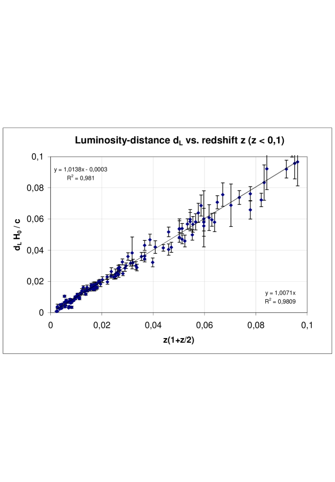
Figure 1: Luminosity distance $d_{L}$ as a function of redshift $z$ for small $z$-values. Sample includes 130 supernovae with $z<0.1$. Luminosity distances and error-bars are taken from [56] and [5]. An unweighted linear regression has been performed on the data, with $y(0)$ fixed to zero (lower right) and $y(0)$ variable (upper left). The respective coefficients of the regression line are shown together with the regression coefficient $R^{2}$.

$d_{L}\widetilde{H_{a}}=z(1+z/2)$ is the dependence of the luminosity-distance in a FRW-universe with zero deceleration parameter. $\widetilde{H_{a}}$ is the value of the Hubble-constant measured via the redshift-distance relation at low redshift. The holostar model of the universe thus predicts a deceleration parameter of zero, i.e. permanently undecelerated expansion. This result is not unexpected. It could have been inferred from the fact, that the active gravitational mass-density within the holostar’s interior space-time is exactly zero, and that the proper geodesic acceleration approaches zero rapidly for large $r$ ($g\propto 1/r^{3/2}$ in the coordinate frame). Note also, that - as was already pointed out in section 2.19 - permanently unaccelerated expansion leads to the prediction $H\tau=1$, which is quite consistent with the WMAP-observations.

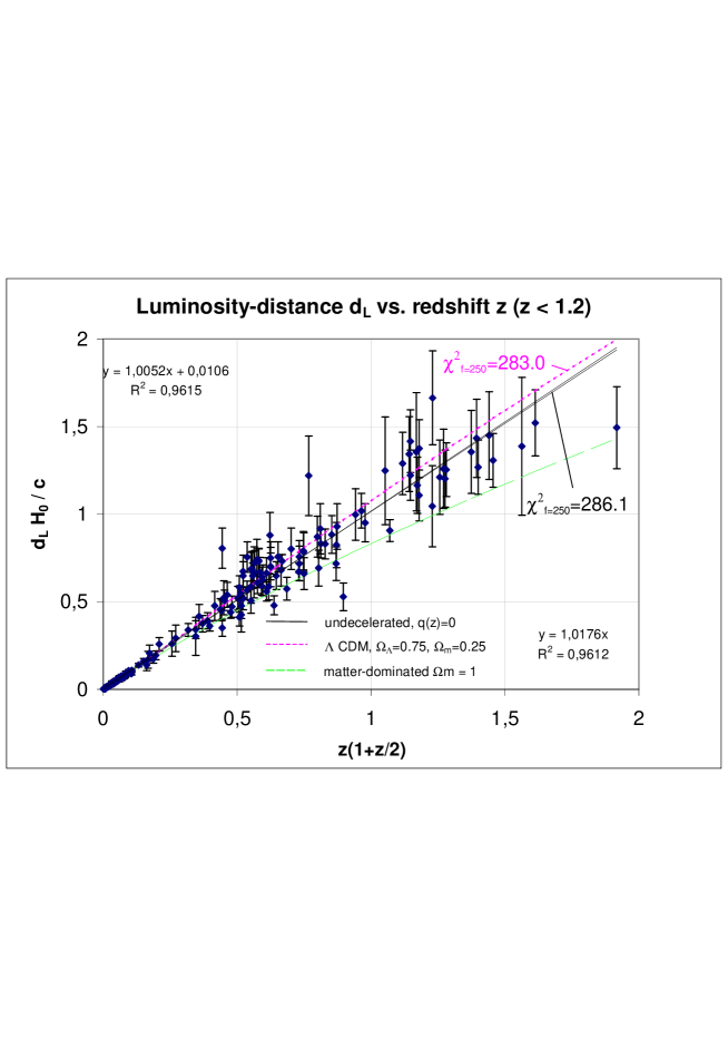
Figure 2: Luminosity distance $d_{L}$ as a function of redshift $z$; full range of $z$-values. Luminosity distances and error-bars are taken from [56] and [5]. The sample includes 253 supernovae with $z<1.2$. The singular high $z$-supernova with $z=1.755$ from [56] is not shown. An unweighted linear regression has been performed on the data, with $y(0)$ fixed to zero (lower right) and $y(0)$ variable (upper left). The respective coefficients of the fit-curves are shown together with the regression coefficient $R^{2}$. The prediction from the standard $\Lambda$-CDM model with $\Omega_{\Lambda}=0.75$ and $\Omega_{m}=0.25$ is shown as dotted line, the prediction for a flat matter-dominated model with $\Omega_{m}=1$ is shown as dashed line.

Figures 1 and 2 show, that the supernova data are compatible with an expansion, that was unaccelerated over the whole $z$-range $0<z<1.2$, well within the measurement errors. Permanently unaccelerated expansion corresponds to a strictly linear dependence in Figures 1 and 2. Due to the large errors it is virtually impossible to decide between the holostar-model (permanently unaccelerated expansion) and the $\Lambda$-CDM models with $\Omega_{\Lambda}+\Omega_{m}\approx 1$ and $\Omega_{m}$ in the range $0.2<\Omega_{m}<0.4$. For instance, the theoretical curve for the $\Lambda$-CDM model with $\Omega_{m}=0.25$ and $\Omega_{\Lambda}=0.75$ is shown in Figure 2 with a dotted line. This line differs from the holostar (straight line) prediction substantially only at large $z>2$, where there are not yet enough data available.

A statistical analysis shows, that it is practically impossible - at least with the current available data and using standard statistical techniques - to make a definite decision in favor of the $\Lambda$-CDM or the holostar model, if one takes the measurement errors into account.

If one uses all data-points of the combined sample of supernova-data ([56] and [5], discarding the three lowest $z$ supernovae, which show very large deviations from the global Hubble-flow) and calculates the $\chi^{2}$-values with respect to the magnitudes predicted by both models, one finds $\chi^{2}=286.1$ for the holostar $q(z)=0$ model and $\chi^{2}=283.0$ for the $\Lambda$-CDM model with $\Omega_{m}=0.25$ and $\Omega_{\Lambda}=0.75$.

For large $N$ the $\chi^{2}$ distribution is quite well approximated by a Gaussian distribution, meaning that the expected outcome of a $\chi^{2}$-test is $f\pm\sqrt{2f}$, where $f$ are the number of degrees of freedom of the distribution. Taking 250 supernova-data one expects $\chi^{2}$ to lie in the range $250\pm 23$. Both models have their $\chi^{2}$ roughly $1.5\,\sigma$ higher than expected. However, one must keep in mind that the (unnormalized) $\chi^{2}$-test only gives correct numbers, when the measurement errors are Gaussian and if one knows the exact value of their Gaussian variance. If the experimenter cannot determine the exact $\sigma_{1}$ Gaussian error, the $\chi^{2}$-value comes out wrong by a constant factor. If the measurement errors are non-Gaussianly distributed (for example because of non-controllable systematics), the Gaussian variance is not a well defined quantity. This is quite evidently the case, as can be seen from the logarithmic plot in Figure 3.

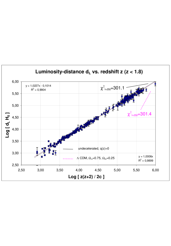
Figure 3: Luminosity distance $d_{L}$ as a function of redshift $z$ in a logarithmic plot; full range of $z$-values. Luminosity distances and error-bars are taken from [56] and [5]. The sample includes all 253 supernovae with $z<1.755$. An unweighted linear regression has been performed on the logarithmic data, with $y(0)$ fixed to zero (lower right) and $y(0)$ variable (upper left). The coefficients of the fit-curves are shown together with the regression coefficient $R^{2}$. The prediction from the standard $\Lambda$-CDM model with $\Omega_{\Lambda}=0.75$ and $\Omega_{m}=0.25$ is shown as dotted line.

Especially the low red-shift data ($N\leq 30$) are problematic. A high percentage of the low-z magnitudes show relative deviations more than a factor 10 higher than the measurement errors. This is incompatible with a Gaussian distribution and points to systematics, such as badly or not compensated peculiar velocities. It is clear, that these data-points will blow up the $\chi^{2}$-value. In a more sophisticated analysis it would be prudent to omit the first 30 or so low $z$ data from the sample. This brings down the $\chi^{2}$ values somewhat closer to the expected range. For $N=224$, i.e. leaving out the first 29 data-points, we find $\chi^{2}_{holo}=230.7$ and $\chi^{2}_{\Lambda CDM}=228.2$.

Although it is - in principle - possible to normalize the $\chi^{2}$-distribution by rescaling the experimentally determined measurement error, I have not done so. Any such rescaling is model-dependent and it is hard to escape unwanted selection effects. The reader therefore has to keep in mind, that the $\chi^{2}$-values quoted in this paper might be off by a constant factor, which is estimated to lie in the range $0.7$ to $1.2$. However, when one tests different theoretical models by a $\chi^{2}$-test, without being sure that the measurement errors are Gaussianly distributed and without being able to put a strong prior on the expected theoretical model, it is not so much the absolute $\chi^{2}$-values, but rather the difference of the $\chi^{2}$-values that is important. Both the holostar- and the $\Lambda$-CDM model fit the data fairly well and their respective $\chi^{2}$-values, although somewhat higher than expected, are so close, that it is not possible to exclude one or the other model by today’s available data. With 220-250 data-points the expected variance of the $\chi^{2}$-test lies between 20-23. Both models differ by $2.5-3$, i.e. roughly one eight of the $\chi^{2}$-variance. Such a small difference cannot be regarded as statistically significant.

In the case of a non-gaussian error distribution a somewhat more robust estimator for the relative error is the absolute deviation. In Figures 3 and 4 the $\chi^{2}$-values were estimated, by summing up the absolute deviations (observed - expected magnitudes) divided by the quoted measurement error, rather than their squares. For large $N$ one can expect this sum to be approximately Gaussian distributed. For a Gaussian distribution the standard deviation is roughly a factor of $1.12$ higher than the absolute deviation. If one estimates a $\chi^{2}$-value by summing up the absolute errors, one will generally underestimate the true $\chi^{2}$-values by approximately this factor.

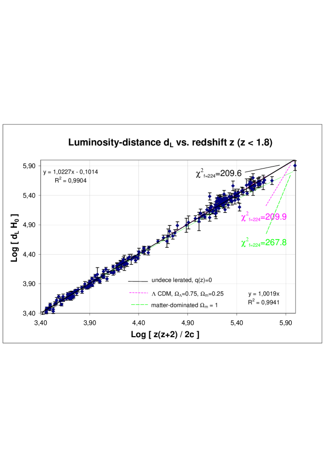
Figure 4: Luminosity distance $d_{L}$ as a function of redshift $z$ plotted logarithmically; the 29 lowest $z$-values were omitted. Luminosity distances and error-bars are taken from [56] and [5]. The sample includes 224 supernovae with $z\leq 1.755$. An unweighted linear regression has been performed on the data, with $y(0)$ fixed to zero (lower right) and $y(0)$ variable (upper left). The respective coefficients of the fit-curves are shown together with the regression coefficient $R^{2}$. The prediction from the standard $\Lambda$-CDM model with $\Omega_{\Lambda}=0.75$ and $\Omega_{m}=0.25$ is shown as dotted line.

This can be seen in the $\chi^{2}$-values of Figure 4. For the 224 high $z$ data points the holostar-model receives $\chi^{2}=209.6$, whereas the $\Lambda$-CDM model has $\chi^{2}=209.9$. Both values are very close to each other and lie 7 % below the expected value $224$ for a genuine $\chi^{2}$-test.

The results of the analysis are summarized in Figure 5, where the observed magnitudes minus the magnitudes expected for permanently undecelerated expansion (= holostar-model) are plotted against red-shift on a logarithmic scale. The holostar-model corresponds to the horizontal line $y=0$. The predictions for the flat $\Lambda$-CDM models with $\Omega_{m}=0.25$ and $\Omega_{m}=0.35$ are shown as dotted and dashed-dotted curves. The curves expected from a flat matter-dominated model ($\Omega_{m}=1$) and a flat vacuum-dominated model ($\Omega_{\Lambda}=1$) are shown as well (lower and upper curve).

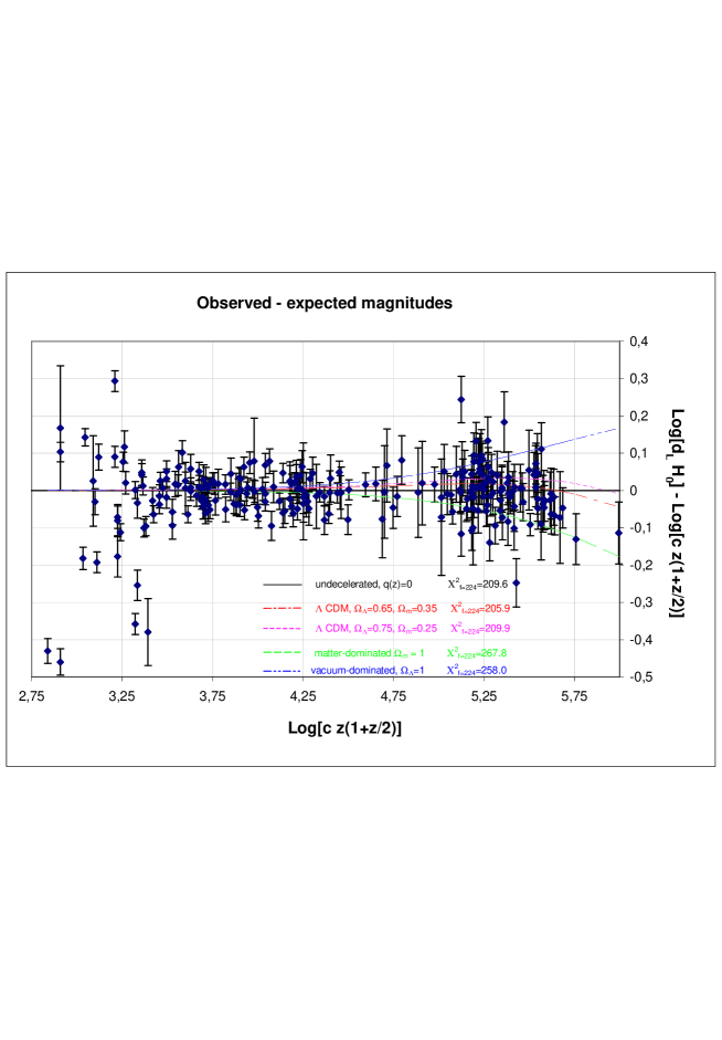
Figure 5: Observed minus expected magnitudes for the full range of $z$-values. The magnitudes and error-bars are taken from [56] and [5]. The sample includes all 253 supernovae with $z\leq 1.755$. The quoted $\chi^{2}$-values refer to the 224 highest $z$-supernovae in the sample. The reference-model (0-line) corresponds to permanently undecelerated expansion. The respective curves for the flat Standard $\Lambda$-CDM model with ($\Omega_{\Lambda}=0.75,\Omega_{m}=0.25$) and ($\Omega_{\Lambda}=0.65,\Omega_{m}=0.35$), as well as the curves for a flat matter-dominated universe (lower curve) and a flat vacuum-dominated universe (upper curve) are shown.

The flat $\Lambda$-CDM model with $\Omega_{m}=0.35$ gives the best $\chi^{2}$-value. The matter-dominated and vacuum dominated models are clearly ruled out by the data. Their respective $\chi^{2}$-values lie three standard deviations higher than the best fitting models.

Although the flat $\Lambda$-CDM model with $\Omega_{m}=0.35$ seems to be slightly preferred, the marginally different $\chi^{2}$-values between the holostar- and the flat $\Lambda$-CDM models in the range $0.2<\Omega_{m}<0.4$ can hardly be regarded as statistically significant, even if one would be willing to accept extremely low confidence levels. It is clear, that in order to rule out one or the other model more high $z$ supernova data are required. For $z>2$ the luminosity red-shift relations of the standard $\Lambda$-CDM models and the holostar-model of the universe differ substantially.

One must also keep in mind, that the so called $K$-corrections relating the observed supernova-intensity in a fixed frequency band to the total bolometric intensity integrated over the whole frequency range is somewhat model-dependent (see for example [8]). Without analysis of the model-dependencies one cannot exclude the possibility of a $z$-dependent systematic error, if one naively interprets the supernova-data in the context of the holostar space-time using the standard $K$-corrections derived in a different context.

The luminosity-distance $d_{L}$ plotted in Figures 1 and 2 is normalized to the Hubble-length $c/\widetilde{H_{0}}$. The Hubble-length cannot be determined by comparing the relative luminosities of the standard candles to their red-shift. In order to determine $\widetilde{H_{0}}$ the absolute magnitude of the standard candles must be known. The absolute magnitude of the SN-1a supernovae has been determined from the first rungs of the cosmological distance ladder, and therefore is subject to the errors within these rungs. On the other hand, a single accurate distance measurement to a nearby supernova, such as SN 1987A, can provide an independent absolute calibration. An analysis of the extended gas envelope of SN 1987A in the large magellanic cloud provides such a means. See [33].

2.21 Structure formation in the holostar space-time

The Hubble law given in equation (110) contains an unknown parameter, the (nearly constant) proper radial coordinate velocity $dr/d\tau\approx\sqrt{r_{0}/r_{i}}$. If the holostar is an appropriate model for the universe, $dr/d\tau$ can be determined by comparing the measured Hubble constant with our current radial coordinate position $r$, which can be estimated from the mass-density. This will be done in section 2.23 and gives $r_{i}\approx r_{0}$, a result that has been hinted already in section 2.12. However, it would be quite helpful if the parameter $dr/d\tau$ could be determined by some independent method. The evolution of the density-fluctuations from the time of decoupling to the structures we find today might provide such a means:

The fluctuations in the microwave background radiation have been determined to be roughly equal to $\delta T/T=10^{-5}$. These small temperature fluctuations are interpreted as the relative density fluctuations at the time of decoupling, i.e. at the time when the microwave background radiation temperature was believed to be roughly 1000 times higher than today. In the adiabatic approach (instantaneous decoupling) the respective fluctuations in the baryon-density at the time of decoupling are $\delta=\delta\rho_{B}/\rho_{B}\approx 3\,\delta T/T$. These fluctuations are believed to have been the seeds of the structure formation process, from which the large scale distribution of galaxies, as we see them today, have formed. The density contrast in the distributions of galaxies on a large scale is roughly of order unity today: $\delta_{today}=\delta\rho/\rho\simeq 1$. In the standard cosmological models this evolution of the density fluctuations is quite difficult to explain. The problem is, that in the dust approximation (no significant pressure, velocity of sound nearly zero), which for a long time was assumed to be the correct description of the universe after decoupling, the fluctuations grow with $\delta\propto t^{2/3}$. In this picture the universe is matter-dominated after decoupling. In a matter-dominated FRW-model we find $r\propto t^{2/3}$. The temperature $T$ and the scale factor $r$ are related by $T\propto 1/r$. Combining these dependencies we get:

$$\delta\propto t^{2/3}\propto r\propto\frac{1}{T}$$ (122)

The above formula predicts $\delta_{today}\approx 10^{-2}$, which is roughly two orders of magnitude less than the observed value.

In order to explain the rather large density fluctuations today, the standard cosmological model has been extended to encompass cold dark matter and - lately - so called ”dark energy”.

In the holostar universe the evolution of the density-fluctuations can be explained quite easily. Only one parameter, the nearly constant radial coordinate velocity $dr/d\tau$ which appears in equation (110) for the Hubble value need to be adjusted.

2.21.1 The evolution of density perturbations in the dust-case

Let us first consider the dust case, i.e. the evolution of the density fluctuations in the holostar by deliberately ignoring the effects of the pressure. The reader should be aware, that this is an unrealistic assumption in the holostar’s interior space-time. The negative radial pressure, equal in magnitude to the matter-density, will always exert a substantial influence on the large scale structure formation. The effect of the pressure will be studied in the subsequent section. We will see that the results for the dust case are almost identical, except for slightly different numerical factors, to the realistic case which includes the pressure.

Far from the starting point of the motion the expansion in the holostar universe (viewed by an observer in the co-moving frame) is very similar to the expansion in the standard Robertson Walker models. The expansion is nearly isotropic. The energy density is matter-dominated over an extended period of time. Therefore the usual standard model formula for the evolution of the density fluctuations should be applicable. In a matter-dominated Robertson Walker universe with zero pressure, the density fluctuations evolve according to the following differential equation (see for example [34]):

$$\ddot{\delta}+2\frac{\dot{r}}{r}\,\dot{\delta}-4\pi\rho\,\delta=0$$ (123)

For the holostar we find:

$$r=\sqrt{\frac{r_{0}}{r_{i}}}\tau$$ (124)

$$\frac{\dot{r}}{r}=\frac{1}{\tau}$$ (125)

$$4\pi\rho=\frac{1}{2r^{2}}=\frac{r_{i}}{2r_{0}}\frac{1}{\tau^{2}}$$ (126)

With these relations equation (123) reduces to the following differential equation:

$$\ddot{\delta}+\frac{2}{\tau}\dot{\delta}-\frac{r_{i}}{2r_{0}}\frac{1}{\tau^{2}}\delta=0$$ (127)

The equation can be solved by the following ansatz:

$$\delta=\tau^{n}$$ (128)

This gives a quadratic equation for $n$

$$n^{2}+n-\frac{r_{i}}{2r_{0}}=0$$ (129)

which can be solved for $n$:

$$n=-\frac{1}{2}\pm\sqrt{\frac{1}{4}+\frac{r_{i}}{2r_{0}}}$$ (130)

In the holographic universe we have the following dependencies:

$$r\propto\tau\propto\frac{1}{T^{2}}$$

Therefore we can express $\delta$ as a function of temperature $T$:

$$\delta\propto\tau^{n}\propto\frac{1}{T^{2n}}\propto\frac{1}{T^{\epsilon}}$$ (131)

with

$$\epsilon=-1\pm\sqrt{1+\frac{2r_{i}}{r_{0}}}$$ (132)

The exponent $\epsilon$ in the above equation can be estimated from the known ratio of the density contrast $\delta_{dec}/\delta_{today}$ and the ratio of the decoupling temperature to the CMBR-temperature.

In the holostar the temperature at decoupling will be larger than in the standard cosmological model, because the number ratio of baryons to photons doesn’t remain constant. If radiation and matter do not interact after decoupling (no re-ionization!), the baryons move geodesically and the baryon number remains constant in the co-moving volume, the baryon-density will scale as $1/r^{3}\propto T^{6}$ in the frame of the co-moving material observer. However, according to the discussion in section 2.28 geodesic expansion against the negative pressure leads to particle creation in the co-moving frame, so that the number-density of the massive particles scales with $1/r^{2}$, if their rest mass remains constant. The baryon-density will scale as $1/r^{2}\propto T^{4}$. Under these circumstances the Saha-equation yields a temperature at decoupling of roughly $T_{dec}\approx 4900K$, when no dark matter component is assumed and the baryon-density today is set to the total matter-density as determined by WMAP [17], i.e. $\rho_{B}=\rho_{m}\approx 2.5\cdot 10^{-27}kg/m^{3}$. A decoupling temperature of $4900K$ corresponds to a red-shift $z_{dec}\simeq 1790$. In order to achieve $\delta_{today}\approx 1$ from $\delta_{dec}\approx 3\cdot 10^{-5}$ at $z_{dec}=1790$, the exponent $\epsilon$ in equation (131) must be roughly equal to $1.48$. For more realistic scenarios in which decoupling doesn’t happen instantaneously $\delta_{dec}$ is estimated to be lower, up to a factor of 10 [50]. For a very slow decoupling scenario with $\delta_{dec}\approx 0.3\cdot 10^{-5}$ we require $\epsilon\approx 1.7$.

For $r_{i}=4r_{0}$ we get $\epsilon=2$, i.e. $\delta\propto 1/T^{2}$, which quite certainly is too high. For $r_{i}=2r_{0}$ we find $\epsilon=\sqrt{5}-1\simeq 1.24$, which is too low. A good compromise is given by $r_{i}\approx 3r_{0}$, which provides a fairly good fit for moderately slow decoupling:

$$r_{i}=3r_{0}\,\rightarrow\,\delta\propto\frac{1}{T^{\sqrt{7}-1}}\simeq\frac{1}{T^{1.65}}$$ (133)

The value $r_{i}=3r_{0}$ is interesting, because for this value the critical mass-energy density in the standard cosmological model, which is given by $\rho_{c}=3H^{2}/(8\pi)$ is exactly equal to the energy density of the holostar, which is given by $\rho=1/(8\pi r^{2})$.

We find that the evolution of the density fluctuations requires $r_{i}\approx 3r_{0}$ and thus $H\approx 0.6/r)$. However, we cannot expect highly accurate results from the above treatment. Although it might be appropriate to ignore the pressure after matter and radiation have become completely decoupled (which might be as low as $z\approx 100$), it is not possible to neglect the pressure in the holostar universe completely. Quite certainly this will not be the case before ”recombination”, i.e. for $z>1800$. If kinematic decoupling happens around $z\approx 100$, the dominant contribution to the evolution of $\delta$ from $z\approx 1800$ (recombination) to $z=1$ (today) falls into an era, where the radiation pressure cannot be neglected.

2.21.2 The evolution of density perturbations in the radiation dominated era

As has been stated before, ignoring the pressure in the holostar space-time is unrealistic. In order to incorporate pressure into the treatment above, we need to know how the anisotropic pressure will manifest itself in the co-moving frame. In [30] universes with anisotropic pressure were studied. The authors found, that an anisotropic pressure will appear as an isotropic pressure for the observer co-moving with the cosmic fluid. The isotropic pressure in the co-moving frame, $P$, is related to the anisotropic pressure components as $P=(P_{r}+2P_{\theta})/3$. If this relation is applied to the holostar, we find $P=-1/(24\pi r^{2})=-\rho/3$. This is the equation of state for an isotropic string gas. Except for the sign the pressure is that of normal radiation. Nonetheless, the sign of the pressure shouldn’t influence the square of the velocity of sound, which is the relevant parameter for the density evolution in a Robertson Walker universe including pressure. Furthermore, the analysis in section 2.9.3 showed that it doesn’t matter, whether one uses the anisotropic holostar pressure or the isotropic radiation pressure of an ultra-relativistic gas in order to calculate the pressure-induced energy change experienced by radiation in geodesic motion. Therefore - whenever matter and radiation cannot be treated as kinematically decoupled - let us make the ansatz, that the density fluctuations in the holostar evolve just as the density fluctuations of a radiation dominated universe. The evolution equation (123) then has to be replaced by:

$$\ddot{\delta}+2\frac{\dot{r}}{r}\dot{\delta}-4\pi\rho\frac{8}{3}\delta=0$$ (134)

If the above equation is expressed in terms of $r_{i}/r_{0}$, the only difference to the dust case in equation (127) is to replace $r_{i}/r_{0}\rightarrow(8r_{i})/(3r_{0})$, so that the exponent in equation (131) is given by:

$$\epsilon=-1\pm\sqrt{1+\frac{16r_{i}}{3r_{0}}}$$ (135)

In order to achieve an exponent of roughly $1.65$ we need $1+16r_{i}/(3r_{0})\approx 7$, which requires

$$\frac{r_{i}}{r_{0}}\approx\frac{9}{8}$$ (136)

Note, that the above value is very close to unity. For $r_{i}=r_{0}$ we find

$$\delta\propto\frac{1}{T^{\sqrt{19/3}-1}}\simeq\frac{1}{T^{1.52}}$$ (137)

which is a good compromise between models assuming instantaneous decoupling ($\epsilon\approx 1.4$) or very slow decoupling ($\epsilon\approx 1.7$).

Equation (135) is quite sensitive to the value of $r_{i}/r_{0}$. It seems quite clear that $r_{i}$ cannot possibly lie outside the range $r_{0}/2<r_{i}<2r_{0}$ in any era, where radiation pressure is significant. If the temperature at decoupling was $4900K$ and decoupling took place very fast, the best fit would be $r_{i}/r_{0}\simeq 0.9$. For non-geodesic motion (after decoupling) one expects that the decoupling temperature will be lower, somewhere in the range between $3500$ and $4900K$. A lower decoupling temperature and non-geodesic motion both require a higher exponent in equation (131), so that $r_{i}\simeq r_{0}$. For non-adiabatic (i.e. not instantaneous) decoupling the baryonic density fluctuations at decoupling have been estimated to be lower (see for example [50]), placing $\delta_{dec}$ in the range $0.3\cdot 10^{-5}<\delta_{dec}<3\cdot 10^{-5}$, in which case $r_{i}/r_{0}$ should be very close to unity.

Whatever the exact value of $r_{i}/r_{0}$ might be, we are drawn to the conclusion that the massive particles making up the matter in our universe must have moved nearly geodesically from $r_{i}\approx r_{0}$. Although the internal logic of the holostar space-time requires $r_{i}\approx r_{0}$, it is difficult to believe this important result without further experimental evidence.

An accurate estimate for the exponent in equation (131) and therefore an accurate prediction for the Hubble-value can only be made if the true equations of motion of massive particles in the holostar space-time, including pressure, are used. However, this requires the inclusion of quantum effects: According to section 2.12 the deviation from pure geodesic motion due to the pressure-forces is completely irrelevant except in the very first stage of the motion, i.e. $r_{i}\leq r<\approx(2-3)\,r_{i}$. But with $r_{i}\approx r_{0}\approx 2\,r_{Pl}$ the motion starts out roughly a Planck distance from the center, where the discreteness of the geometry and quantum effects will come into play. A detailed analysis of the motion of particles in the holostar, including the region close to its center, therefore must be left to future research.

2.22 On the angular correlation of the CMBR

As has already hinted in footnote 61 the experimentally determined ratio $r_{i}/r_{0}\approx 1$ only makes sense, if the particles in the universe - as we see it today - have originated from a few Planck-distances from the holostar’s center. A rather conservative scenario within this line of thought is, that a - presumably massive - precursor particle was created close to the center and then moved out on a nearly geodesic trajectory henceforth. Nearly geodesic motion through the hot interior region of the holostar space time, starting out from $r\approx r_{0}$, seems only conceivable for a massive particle of roughly Planck mass which only interacts weakly with the other particles. Somewhere on its trajectory, not too far from the radial coordinate value where the temperature has dropped below the electro-weak unification scale, the particle (or its intermediate decay products) must have decayed into ordinary matter, endowing the stable final products (electrons, protons, neutrons and neutrinos - or more generally the light quark/leptons) with the high momentum gathered on its outward track. This scenario - although well within the limits of standard physics - is quite an extravagant claim, for which it would be helpful to have another - independent - verification. The missing angular correlation of the microwave background radiation at large angular separations might provide such a means.

The low quadrupole and octupole moments of the CMBR as determined from of the WMAP data [17] demonstrate, that there is practically no correlation between the fluctuations in the microwave background radiation at angular separations larger than approximately $60^{\circ}$, which corresponds to roughly $1$ radian. This feature can be quite effortlessly explained by the motion of massless and massive particles in the holostar space-time

2.22.1 Limits on the angular motion of massive particles

As can be seen from equation (28) particles that were emitted just a few Planck distances from the center have limited angular spread. According to the scenario proposed beforehand let us assume, that a massive particle is created with not too high a tangential velocity $\beta_{i}$ close to the center of the holostar. The particle must not necessarily have a long life-time. Any decay products will follow the original trajectory. The maximum angular spread of the particle (or of its decay products) can be calculated:

$$\varphi_{max}=\beta_{i}\sqrt{\frac{r_{i}}{r_{0}}}\int_{0}^{1}{\frac{dx}{\sqrt{1-x\left(1-\beta_{i}^{2}(1-x^{2})\right)}}}=\beta_{i}\sqrt{\frac{r_{i}}{r_{0}}}\,\xi(\beta_{i}^{2})$$ (138)

$\xi=\xi(\beta_{i}^{2})$ depends on the tangential velocity $\beta_{i}$ at the turning point of the motion. As remarked in section 2.6, $\xi$ lies between $1.4<\xi\leq 2$, depending on $\beta_{i}$. Equation 138 gives an implicit relation for $\beta_{i}^{2}$ , which can be solved iteratively for $\beta_{i}^{2}$, whenever the maximum angular spread $\varphi_{max}$ and the ratio $r_{i}/r_{0}$ is known.

$\varphi_{max}$ and $r_{i}/r_{0}$ can be determined experimentally. However, there is a subtlety involved in the experimental determination of $r_{i}/r_{0}$ from the characteristics of the expansion. The derivation of equation (110) for the Hubble-value relies on the - implicit - assumption, that the motion started out from $r_{i}$ at rest. This is unrealistic. At $r_{i}\approx r_{0}$ there is an extremely high temperature, so that even a particle of nearly Planck mass will have an appreciable velocity at its (true) turning point of the motion, $r_{i}$. Therefore the ratio $r_{i}/r_{0}$ in equation (110) doesn’t refer to the true turning point of the motion $r_{i}$, but rather to a fictitious ”zero-velocity” turning point $\widetilde{r_{i}}$, which describes the radial part of motion far away from the turning point. Both values are related: In section 2.6 it has been shown, that the radial part of the motion of a particle with an appreciable tangential velocity at its turning point is nearly identical to the motion of a particle that started out from a somewhat smaller radial coordinate value, whenever $r\gg r_{i}$. The relation between the true turning point $r_{i}$ of the motion and the apparent (zero-velocity) turning point $\widetilde{r_{i}}$ measured at large distances is given by:

$$r_{i}=\gamma_{i}^{2}\widetilde{r_{i}}$$ (139)

where $\gamma_{i}$ is the special relativistic $\gamma$-factor of the particle at its true turning point of the motion.

The experimentally determined ratio $r_{i}/r_{0}$ in the Hubble equation (110) or in the equation for the density evolution (134) therefore rather refers to $\widetilde{r_{i}}/r_{0}$, whereas $r_{i}$ in equation (138) refers to the true turning point of the motion. In section 2.21 this ratio has been estimated as $\widetilde{r_{i}}/r_{0}\approx 1$, if the density perturbations found in the microwave background radiation $\delta\approx 10^{-5}$ evolve according to equation (131) in combination with equation (135) to the value observed today. Let us denote the experimentally determined ratio with $\kappa$:

$$\kappa=\frac{\widetilde{r_{i}}}{r_{0}}=\frac{1}{\gamma_{i}^{2}}\frac{r_{i}}{r_{0}}$$ (140)

The equation for the maximum angular spread then reads:

$$\varphi_{max}^{2}=\beta_{i}^{2}\xi^{2}(\beta_{i}^{2})\frac{r_{i}}{r_{0}}=\beta_{i}^{2}\gamma_{i}^{2}\xi^{2}(\beta_{i}^{2})\kappa$$ (141)

so that:

$$\beta_{i}^{2}\gamma_{i}^{2}=\frac{\beta_{i}^{2}}{1-\beta_{i}^{2}}\simeq\frac{\varphi_{max}^{2}}{\xi^{2}(\beta_{i}^{2})\kappa}$$ (142)

Whenever we know $\kappa$ and $\varphi_{max}$, the tangential velocity at the true turning point of the motion $\beta_{i}$ follows from equation 142) . Knowing $\beta_{i}$ the true turning point of the motion can be determined

$$r_{i}=\gamma_{i}^{2}\widetilde{r_{i}}=(1+\beta_{i}^{2}\gamma_{i}^{2})\kappa r_{0}$$ (143)

where the relation $\gamma^{2}=1+\beta^{2}\gamma^{2}$ was used.

For $\varphi_{max}=60^{\circ}=\pi/3\approx 1$ the maximum angular spread is nearly unity (in radians). For $\kappa=1$ we find $\xi\approx 1.77$. With these values

$$\beta_{i}^{2}\gamma_{i}^{2}\simeq 0.319$$ (144)

so that

$$\beta_{i}^{2}=\frac{\beta_{i}^{2}\gamma_{i}^{2}}{1+\beta_{i}^{2}\gamma_{i}^{2}}\simeq 0.242$$ (145)

and

$$\frac{r_{i}}{r_{0}}\simeq 1.319$$ (146)

If we know $\beta$ and the momentum $p$ of a massive particle at the radial position $r_{i}$, where the particle’s motion has become nearly geodesical, we can determine the mass of the particle. The momentum of any massive particle is related to its mass $m_{0}$ by

$$p=\beta\gamma m_{0}$$ (147)

To determine $m_{0}$ we need $p$. Any massive particle at the holostar’s center will be immersed in a very hot radiation bath of ultra-relativistic or zero rest mass particles. It seems reasonable to assume, that at position $r_{i}\approx r_{0}$, where the particle starts to move out geodesically, the thermal radiation will have imprinted its momentum on the massive particle. In the holostar the mean momenta $\overline{p}_{\gamma}$ of the ultra-relativistic particles are proportional to the interior radiation temperature, given by equation (57).

$$\overline{p}_{\gamma}=\sigma_{S}T_{\gamma}=\frac{\sigma_{S}}{4\pi}\frac{\hbar}{\sqrt{r_{i}r_{0}}}$$ (148)

In [41] it is shown, that the factor of proportionality $\sigma_{S}$ is equal to the entropy per particle (which is slightly larger than $\pi$ for a great variety of circumstances). Putting all equations together and using the relation $r_{0}^{2}/\hbar\approx 4\sigma_{S}/\pi$ at the Planck-energy proposed in [39] we find:

$$m_{0}\simeq\frac{1}{8}\sqrt{\frac{\sigma_{S}}{\kappa\pi}}\frac{\sqrt{\hbar}}{\beta_{i}\gamma_{i}^{2}}$$ (149)

With $\kappa=1$ and $\varphi_{max}=1$ the mass of the precursor particle $m_{0}$ is given by:

$$m_{0}\simeq 0.201\,m_{Pl}$$ (150)

We have used $\sigma_{S}=3.38$, which is the mean entropy per ultra-relativistic particle, when the ultra-relativistic particles at the Planck-temperature are predominantly fermions. For a more detailed discussion of how $\sigma_{S}$ can be derived from microscopic statistical thermodynamics see [41].

2.22.2 The preon - a massive particle of roughly Planck mass?

It appears, that in order to explain the missing angular correlation in the CBMR at large angular separations we require a heavy precursor particle of roughly a fifth of the Planck mass. Lets call this particle the ”preon”.

Let us assume that the preon is created close to the holostar’s center. Due to $\overline{p}_{\gamma}=\sigma_{S}T_{\gamma}=\sqrt{\sigma_{S}/\pi}/4\approx 0.561\,m_{0}\approx 0.113\,m_{Pl}$ the preon-production will be somewhat inhibited at at $r_{i}\approx 1.3\,r_{0}$, as an energy of $E=\sqrt{\overline{p_{\gamma}}^{2}+m_{0}^{2}}\approx 0.231\,m_{Pl}$ is required. However, at $r=r_{0}/2\approx r_{i}/2.6$ there is just enough energy available to create preons in (in pairs) in substantial numbers, either by the collision of any two massive or massless particles of the surrounding radiation bath, or - slightly more efficiently - by Unruh radiation: At a radial coordinate position $r=r_{0}/2$ the local radiation temperature $T_{\gamma}$ will be up by a factor of $\sqrt{2.6}$ with respect to the temperature at $r_{i}$, so that the mean momentum of the radiation will be given by $\overline{p}_{\gamma}\approx 0.183\,m_{Pl}$. The mean energy of the (massive) preon at $r_{0}/2$ will be higher as well, but not with the same factor as the radiation, because of its non-negligible rest-mass. We find: $E_{0}\approx\sqrt{\overline{p_{\gamma}}^{2}+m_{0}^{2}}\approx 0.272\,m_{Pl}$. The mean momentum of the radiation quanta doesn’t yet suffice to produce the preon efficiently in pairs, at least not with the right momentum. However, the mean energy of the two radiation quanta is almost large enough to produce two preons with zero momentum.

Presumably the most efficient way to produce preons is via Unruh radiation between $r_{0}/2<r<r_{0}$. The Unruh-temperature at $r=r_{0}/2$ will be twice the radiation temperature (see section 2.30). The energy of a particle produced by Unruh radiation therefore is $E\approx 0.366\,m_{Pl}\approx 1.35\,E_{0}$. The production of a preon by Unruh radiation poses no problem, even if the high chemical potential of the ultra-relativistic particles, $\mu>1.34\,T_{\gamma}$, in the holostar is taken into account.

So far the case $\kappa=\widetilde{r_{i}/r_{0}}=1$ was discussed. The mass of the preon $m_{0}$ depends on $\kappa$, albeit only moderately. If $\kappa$ lies in the range $0.5<\kappa<4$ we find the following mass-range:

$$0.164<m_{0}<0.243$$ (151)

in Planck units.

In Table 1 the mass $m_{0}$ and the tangential velocity $\beta_{i}$ of the preon is given for several values of $\kappa$:

$\kappa$	$\beta_{i}$	$\xi$	$m_{0}$
1/2	0.647	1.65	0.165
3/4	0.553	1.72	0.188
1	0.490	1.77	0.201
3/2	0.405	1.83	0.218
2	0.353	1.87	0.228
5/2	0.316	1.89	0.234
3	0.288	1.91	0.238
4	0.250	1.93	0.243

Table 1: preon mass $m_{0}$ as a function of $\kappa$; $\varphi_{max}=56.8^{\circ}$

If equation (134) for the density evolution (with pressure) is correct, $\kappa$ should lie in the range $3/4<\kappa<5/4$, so that the bound for the preon mass will be roughly $0.19<m<0.21$ in Planck units. $\kappa\approx 1$ also fits better with the current measurements of the Hubble-constant (see section 2.23).

We find, that if the current expansion rate of the universe and the evolution of the density perturbations after decoupling can be (approximately) described by the holostar solution, one requires a new particle. Its properties can be quite accurately inferred from the above discussion: Its mass should be less than one quarter of the Planck mass. Its exact value shouldn’t lie too far outside the mass range given by equation (151). The particle - or its decay products - should interact only weakly with the other particles at energies above the electro-weak scale.

2.22.3 An independent estimate for the preon mass

It is possible to estimate the mass of the preon by another, independent argument. According to the discussion in section 2.22.7 the proper volume occupied by a single particle at the holostar’s center is given by

$$V_{1}=\int_{0}^{r_{0}/2}{dV}=\frac{8\pi}{7\sqrt{2}}\left(\frac{r_{0}}{2}\right)^{3}\approx\frac{8\pi}{7\sqrt{2}}V_{Pl}$$ (152)

On its way outward the volume available to the preon will become larger, which enables it to decay into lighter particles, such as neutrons, protons and electrons. The decay is expected to conserve mass-energy locally. What will the energy-density of the stable decay products be at large $r$-values? To simplify the calculations it is convenient to consider a thought-experiment, in which the proper expansion in the radial direction is zero. This thought-experiment simplifies the calculations as we don’t have to take into account any changes of the internal energy in a radially expanding volume due to the non-zero radial pressure. Any motion leaving the internal energy of a spherically outmoving shell of particles unaffected, requires that the proper thickness of the shell remains constant, i.e. the volume develops as the proper surface area of the concentric spherical shell, i.e. $V\propto r^{2}$.

At the radial position $r=9.18\cdot 10^{60}\,r_{Pl}$, which corresponds to the radius of the observable universe today, the volume $V_{1}$ will have expanded to:

$$V_{today}=\left(\frac{r}{r_{Pl}}\right)^{2}V_{1}\simeq 1.0\cdot 10^{18}m^{3}$$ (153)

Assuming local mass-energy conservation and assuming that the mass-energy of the preon ends up predominantly in nucleons (i.e. no significant dark matter component; energy-contributions of electrons, neutrinos and photons negligible with respect to the baryons), the total number of nucleons within this volume will be given by:

$$N_{n}=\frac{E_{preon}}{m_{p}}\approx 1.68\cdot 10^{18}$$ (154)

if the mass-energy of the preon is assumed to be $E_{preon}=p_{\gamma}(r_{0})\simeq\sqrt{\sigma_{S}/\pi}\,m_{Pl}/8=0.13\,m_{Pl}$. From equations (153, 154) the number-density of nucleons in the universe today can be estimated as:

$$n_{n}=1.68\frac{1}{m^{3}}$$ (155)

amounting to roughly $1.7$ nucleons per cubic meter. This is very close to the number-density of nucleons in the universe derived from the total matter-density determined by WMAP assuming no significant dark matter component, $n_{n}=1.48/m^{3}$ (see section 2.23). Therefore a preon-mass in the range between $0.1$ to $0.2$ Planck masses is quite consistent with the findings in the observable universe today.

2.22.4 An estimate for the amplitude of the density perturbations

The assumption that the preon eventually decays into nucleons at a temperature slightly below the nucleon rest-mass, enables us to give a - very crude - estimate for the absolute value of the density contrast $\delta$ at the time of baryogenesis. Astoundingly this crude estimate fits quite well with the experimentally determined values of the density contrast today $\delta_{today}\approx 1$ and at the time of decoupling $\delta_{dec}\approx 10^{-5}$:

The red-shift $z_{b}$ where the mean energy of the radiation is equal to the nucleon rest-mass is given as:

$$z_{b}\approx\frac{m_{p}/3.37}{T_{CMBR}}\approx 1.19\cdot 10^{12}$$ (156)

At this redshift the number-density of the nucleons $n_{b}$ in the holostar space-time will be higher than today by a factor of $z_{b}^{4}$, i.e.

$$n_{b}\approx\frac{1.5}{m^{3}}z_{b}^{4}\approx\frac{3\cdot 10^{48}}{m^{3}}$$ (157)

which corresponds to a matter-density of $\rho_{b}\approx 5\cdot 10^{21}kg/m^{3}$. This value is roughly a factor of thousand higher than the typical neutron star density and four orders of magnitude higher than the typical density of stable nuclei.

If the nucleons in our universe originate from the preon at roughly this redshift, one would expect a density-contrast $\delta_{b}$ on the order of the nucleon to preon mass at this time. With a preon mass $m_{preon}\approx 0.15\,m_{Pl}$ we find

$$\delta_{b}\approx\frac{m_{p}}{m_{preon}}\approx 5\cdot 10^{-19}$$ (158)

As has been shown in section 2.21 the density contrast evolves as a power-law with respect to the redshift. For $\kappa=1$ the exponent is given by $\epsilon=\sqrt{19/3}-1\simeq 1.517$ in the radiation dominated era, so that:

$$\delta\propto\frac{1}{z^{1.517}}$$ (159)

Therefore we can ”predict” the density-contrast at any redshift $z<z_{b}$ from the density-contrast at the time of baryogenesis. We find:

$$\delta_{dec}=\delta_{b}\left(\frac{z_{b}}{z_{dec}}\right)^{1.517}\approx 1.2\cdot 10^{-5}$$ (160)

with $z_{dec}\approx 1800$ and

$$\delta_{today}=\delta_{b}\left(\frac{z_{b}}{1}\right)^{1.517}\approx 1.05$$ (161)

However, keep in mind that as long as not much is known about the particle spectrum at energies above the electro-weak scale this ”prediction” stands on more than shaky ground.

2.22.5 A string explanation for the CMBR power spectrum

The string-character of the holostar space-time allows an alternative explanation, not only for the absolute value of the density perturbations but also for the scale-invariant spectrum of the CMBR-fluctuations found by WMAP. As this has been discussed elsewhere, I will just give a very short summary of the presentation in Peacock [34, p. 316-321]:

It is easy to see, that the holostar’s interior space-time can be interpreted as a collection of strings, aligned in the radial direction. For a string-dominated universe one finds the following rough estimate for the horizon-scale amplitude $\delta_{H}$:

$$\delta_{H}=\left(\frac{\delta\rho}{\rho}\right)_{H}\approx\left(\frac{E_{GUT}}{E_{Pl}}\right)^{2}$$ (162)

As $E_{GUT}\approx 10^{-3}E_{Pl}$ numbers close to the characteristic value $\delta_{H}\approx 10^{-5}$ can arise quite naturally.

Because of the way in which the string network scales, the density perturbations generated by stringy matter have an approximately scale invariant spectrum. However, string structure formation is generally non-Gaussian in nature. Therefore it might be possible to detect a non-Gaussian string signature in the small-scale CMBR anisotropies

2.22.6 Limits on the angular motion of photons - an estimate for the maximum angular correlation distance

So far the maximum angular correlation distance of the microwave background radiation ($\varphi_{max}\approx 60^{\circ}$) has been put in by hand, as determined from the observations. It would be nice, if this value could be derived by first principles. There appears to be a way to do this. For this purpose let us consider the angular spread of zero mass particles in the holostar. The maximum angular spread for a photon emitted from $r_{i}$ is given by:

$$\varphi_{max}=\frac{\sqrt{\pi}}{3}\frac{\Gamma(\frac{1}{3})}{\Gamma(\frac{5}{6})}\sqrt{\frac{r_{i}}{r_{0}}}\simeq 1.4022\sqrt{\frac{r_{i}}{r_{0}}}$$ (163)

Let us consider photon-pair production (or the production of any other massless particle in pairs) by Unruh radiation. This process will be most efficient if the Unruh-temperature is high. In section 2.30 the following relation between radiation temperature and Unruh-temperature will be derived:

$$\frac{T_{U}}{T_{\gamma}}\simeq\frac{r_{0}}{r}$$ (164)

For $r_{i}=r_{0}/2$ the Unruh temperature is twice the radiation temperature, so that photon pair production by the Unruh-effect should be a common occurrence in the central region of the holostar. Unruh creation of photon pairs is most efficient at the most central conceivable location available for a particle within the holostar space-time. According to the discussion in section 2.22.7 there are many good reasons to believe, that $r_{i}=r_{0}/2$ is the ”closest” conceivable position that any one particle can occupy at the holostar’s center. If we insert the ratio $r_{i}/r_{0}=1/2$ into equation (163) we get:

$$\varphi_{max}=\frac{\Gamma(\frac{1}{3})}{\Gamma(\frac{5}{6})}\sqrt{\frac{\pi}{18}}\simeq 0.9915=56.81^{\circ}$$ (165)

Voil$\grave{a}$.

Finally it should be noted, that $\varphi_{max}\approx 1$ makes the ”expansion” of particles that move radially outward in the holostar space-time nearly equal in the radial and the tangential directions: $\delta l_{\perp}=r\varphi_{max}$, whereas $\delta l_{r}\approx r$.

2.22.7 Applying the uncertainty principle to the holostar’s central region

If one compares the theoretical prediction for the Hubble constant, the theoretical prediction for the evolution of the density perturbation amplitudes and maximum correlation angle with the cosmological observations, all methods favor $r_{i}\approx r_{0}$, meaning that the particles making up our universe must have originated from a region $r_{0}/2<r_{i}<2r_{0}$. Is it conceivable, that the particles could have originated from an interior position very much closer to the center?

It is easy to see that the answer is no. Any particle located close to the holostar’s center will have a mean momentum comparable to the Planck-momentum. However, any particle must be subject to the Heisenberg uncertainty relation. If we set the momentum uncertainty $\Delta p$ of the particle equal to its mean (thermal) momentum at $r_{i}$, and the uncertainty in position $\Delta r_{i}$ equal to to $r_{i}$, the uncertainty relation reads:

$$\Delta p\,\Delta r_{i}=\frac{\sigma_{S}}{\pi}\frac{\hbar}{4}\sqrt{\frac{r_{i}}{r_{0}}}\geq\frac{\hbar}{2}$$ (166)

With $\sigma_{S}\approx\pi$ we find the following inequality for $r_{i}/r_{0}$:

$$\frac{r_{i}}{r_{0}}\geq 2$$ (167)

Quite evidently this is not an exact result, as $\Delta p\neq p$ and $\Delta r_{i}\neq r_{i}$. Still one can expect this relation to be correct within a factor of two or three. We find that any particle in the holostar’s center will not be able to occupy a region (or originate from a region) much smaller than $r\approx r_{0}$.

There are some other independent reasons to believe, that $r_{0}$ - or rather $r_{0}/2\approx\sqrt{\hbar}$ - provides a universal cut-off for the region that can by occupied by any one particle in the holostar space-time.

First, it does not seem possible that more than one particle will be able to enter - or occupy - the region bounded by the smallest possible area quantum of loop quantum gravity, which turns out to be roughly equal to $4\pi(r_{0}/2)^{2}$ (see [39]). Therefore the smallest ”separation” between two particles should be roughly equal to $r_{0}$, as far as semi-classical reasoning can still be trusted at the Planck scale.

Second, in [41] the number of particles within a spherical concentric region in the holostar space-time has been determined as $N=(\pi/\sigma_{S})\,(r^{2}/\hbar)\simeq r^{2}/\hbar$ (as $\sigma_{S}\approx\pi$). This relation was derived in the context of microscopic statistical thermodynamics, which generally requires macroscopic $N$. Extrapolating this relation to the Planck-scale using the experimental estimate $r_{0}\approx 2\sqrt{\hbar}$ from equation (60) we find that $N\simeq 1$ for $r=r_{Pl}\approx r_{0}/2$.

A third argument is this: In [39] it has been shown, that $r_{0}/2$ is the radial position of the membrane of an elementary extremely charged holostar with zero (or negligible) mass. A holostar with $r_{h}=r_{0}/2$ is the smallest holostar possible: Any holostar with $r_{h}<r_{0}/2$ necessarily has negative mass.

Therefore any particle coming from the holostar’s hot central region will appear to have originated from $r_{i}\approx r_{0}$ for an observer situated a large distance from the center. Whether the particle was created at the hot central region, or whether an inmoving particle merely reversed its motion at $r\approx r_{0}$ (or was reflected from the center by a small angle) is quite irrelevant to the general picture.

2.23 Estimating cosmological parameters from the radiation temperature

In this section the total local mass-energy density $\rho$, the local Hubble value $H$, the radial coordinate value $r$ and the proper time $\tau$ in a ”holostar universe” will be determined from the temperature of the microwave background radiation.

The total energy density in the holostar universe can be determined from the radiation temperature, whenever $r_{0}^{2}$ is known. It is given by equation (58):

$$\rho=\frac{2^{5}\pi^{3}r_{0}^{2}}{\hbar^{4}}T^{4}$$ (168)

There is some significant theoretical evidence for $r_{0}^{2}\approx 4\sqrt{3/4}\hbar$ at the low energy scale. However $r_{0}^{2}=4\hbar$ or a value a few percent higher than $4\hbar$ might also be possible (for a somewhat more detailed discussion see [39]). With $r_{0}^{2}=4\sqrt{3/4}\hbar$ and $T_{CMBR}=2.725K$ we find:

$$\rho=2.425\cdot 10^{-27}\frac{kg}{m^{3}}=1.450\cdot\frac{m_{p}}{m^{3}}=4.702\cdot 10^{-124}\rho_{Pl}$$ (169)

This is almost equal to the total matter-density of the universe determined by WMAP [17]:

$$\rho_{WMAP}=2.462\cdot 10^{-27}\frac{kg}{m^{3}}$$ (170)

From the matter density the radial coordinate position $r$ within the holostar can be determined.

$$r=\frac{1}{\sqrt{8\pi\rho}}=9.199\cdot 10^{60}r_{Pl}=1.575\cdot 10^{10}ly$$ (171)

This value is quite close the radius of the observable universe.

The local Hubble-constant can be determined from the matter density via equation (110):

$$H=\sqrt{8\pi\rho\frac{r_{0}}{r_{i}}}$$ (172)

With $r_{i}/r_{0}=1$ and the matter density determined beforehand we find:

$$H=2.021\cdot 10^{-18}\,[\frac{1}{s}]=62.36\,[\frac{km/s}{Mpc}]$$ (173)

The Hubble-constant comes out quite close to the value that is used in the concordance model by the WMAP-group [17] with $H=71\,km/s\,/Mpc$. This is an encouraging result. Note, however, that the value of the Hubble constant is model-dependent. It is possible to relate the Hubble value $H_{s}$ of the various versions of the standard cosmological models to the Hubble value $H_{h}$ of the holostar solution via the mass-density. In the standard cosmological models we find:

$$\rho_{m}=\Omega_{m}\rho_{c}=\Omega_{m}\frac{3H_{s}^{2}}{8\pi}$$ (174)

For the holostar the mass-density is given by

$$\rho_{m}=\frac{r_{i}}{r_{0}}\frac{H_{h}^{2}}{8\pi}$$ (175)

Setting the mass densities equal, the local Hubble-values can be related:

$$H_{h}^{2}=\Omega_{m}\frac{3r_{0}}{r_{i}}H_{s}^{2}$$ (176)

Both values are equal, if $\Omega_{m}=r_{i}/(3r_{0})$. This is almost the case for $\Omega_{m}\approx 0.26\approx 1/4$ according to WMAP and $r_{i}/(3r_{0})\approx 1/3$ as determined in section 2.21. This result is quite robust. If we determine $H_{h}$ from $H_{s}$ via equation (176) for various combinations of $\Omega_{m}$ and $H_{s}$ that have been used in the past we get the result of equation (173) with an error on the order of a few percent.

From the local Hubble-value determined in (173) the proper time $\tau$, which can be interpreted as the ”age” of the universe, can be derived:

$$\tau=\frac{1}{H}=9.180\cdot 10^{60}t_{Pl}=1.57\cdot 10^{10}y$$ (177)

This is somewhat larger than the result recently announced by the WMAP group, $t=1.37\cdot 10^{10}y$. Keep in mind, however, that the WMAP-result for the age of the universe is strongly correlated with the prior on the Hubble-constant via the relation $Ht\approx 1$. In fact, it is the product $Ht$ which has been determined to the remarkably high accuracy stated by the WMAP group. In order to determine $H$ or $t$ individually to the same accuracy, independent measurements for $H$ (or $t$) are required, such as provided by the concordance model.

If we set $r_{i}/r_{0}=3/4$ we find an almost perfect agreement of the holostar’s predictions for the local Hubble value $H_{h}=71.85$ (km/s)/Mpc and the current proper time $\tau=13.6\,Gy$ compared to the values determined by WMAP [17], $H=71$ (km/s)/Mpc and $t=13.7\,Gy$.

The holostar solution is quite compatible with the recent findings concerning the large scale structure and dynamics of the universe. The recent WMAP results are reproduced best by setting $\kappa=r_{i}/r_{0}=3/4$. From the evolution of the density perturbations (see section 2.21) one would rather expect $r_{i}\simeq r_{0}$. It is quite clear that $r_{i}/r_{0}$ cannot lie very much outside the range $3/4<r_{i}/r_{0}<1$, which corresponds to an age of the universe in the range between $13-16\,Gy$.

Note that the above age comes close to the ages of the oldest globular clusters. If $r_{i}/r_{0}$ is chosen larger than unity, the proper time $\tau$ in the holostar universe will be larger. For $r_{i}/r_{0}\approx 2$ the holostar universe can easily accommodate even the old estimates for the ages of the globular clusters, which not too far ago have been thought to lie between $13$ to $19$ billion years. The problem with such an assignment is, that the Hubble value comes out far too low. For $r_{i}=2r_{0}$ we find $H\approx 44$ (km/s)/Mpc, which appears incompatible with today’s experimental measurements, even if the large systematic errors in calibrating the cosmological distance scale are taken into account.

From a theoretical point of view $r_{i}=r_{0}$ appears as the most preferable choice (see for instance the discussion in section 2.30). However, this choice is based on an extrapolation of the classical geodesic equations motion from large distances back to roughly a Planck distance from the holostar’s center. It is questionable whether classical reasoning at the Planck-energy scale will remain valid, so that one should expect some moderate adjustment due the quantum nature of space-time at this scale. Therefore it is too early to make a definite numerical prediction for the ratio $r_{i}/r_{0}$ (measured via the Hubble-constant at late times). If $r_{i}/r_{0}$ can be pinned down theoretically we are in the very much desirable position to make a precise prediction for the Hubble value, which should be an order of magnitude better than today’s measurement capabilities. Therefore any significant advances in the understanding of the motion of particles in the holostar universe could be of high practical value for the development of a ”high precision cosmology” in the near future.

2.24 A determination of the local entropy density

Another important quantity that can be determined from the the radiation temperature is the entropy density $s$. According to equation (94) the entropy-density is given by:

$$s=\frac{g}{\hbar}=\frac{1}{2r\hbar}\sqrt{\frac{r_{0}}{r}}$$ (178)

Replacing $r$ with the radiation temperature via equation (57) we find:

$$s=\frac{4r_{0}^{2}}{\hbar}\left(\frac{2\pi T}{\hbar}\right)^{3}$$ (179)

With $r_{0}^{2}/\hbar=4\sqrt{3/4}$ and inserting the CMBR-temperature we get the following prediction for the local entropy-density:

$$s=\frac{5.817\cdot 10^{12}}{m^{3}}=\frac{2.454\cdot 10^{-92}}{r_{Pl}^{3}}$$ (180)

It appears, that this entropy density is quite in conflict with the entropy-density in our universe, which - according to the common belief - is thought to be dominated by the entropy in the CMBR-radiation. The entropy-density of the CMBR is roughly three orders of magnitude lower, $s_{\gamma}\approx 1.5\cdot 10^{9}/m^{3}$. However, this point of view does not take the entropy of the nucleons (and electrons) properly into account. It is a - strangely - utterly ignored result from microscopic statistical thermodynamics, that the entropy $\sigma_{m}$ per massive particle in the non-relativistic limit is given by:

$$\sigma_{m}=\frac{m-\mu}{T}+\frac{5}{2}=\frac{\epsilon-\mu}{T}+1$$ (181)

in units ($c=k=1$). See [34, p. 277] for an approximate derivation when $\mu=0$ and [43] for a full derivation. $\epsilon$ is the total energy per particle, including the kinetic energy $\epsilon=m+(3/2)\,T$.

If one assumes $\mu\approx\epsilon\approx m$ for massive particles, the entropy per massive particle remains small. In a self-consistent space-time, i.e. a space-time that can be considered to be a closed thermodynamical system to a good approximation, this assumption quite likely is not correct. For instance, for a spherically symmetric black hole we know that the entropy is a function of the energy alone $S=S(E)$. The number of particles within a black hole is undefined. But the chemical potential is defined as the energy change at constant entropy, when a particle is added to the system. For a spherically symmetric black hole this energy-change is zero: Adding a particle at constant entropy does not change the total energy of the system, because of the definite relation $E=E(S)$. Therefore the chemical potential of the ”interior particles” must be zero. Something similar applies to the holostar. A holostar has a definite number of particles - at least on average and at high temperatures. But again there is a definite relation between total mass $M$, temperature at infinity $T$ and entropy, i.e. $S\propto M^{2}\propto M/T$. As long as the total mass-energy of the holostar does not change, the total entropy remains constant. Therefore any internal fluctuations of particle-numbers neither change the total energy, nor the total entropy of the whole system. The chemical potential should be zero.

Somewhat more formally:

$$dE=\frac{\partial E}{\partial S}dS+\frac{\partial E}{\partial N}dN+\frac{\partial E}{\partial V}dV+X_{i}dx_{i}$$

$X_{i}dx_{i}$ refer to exterior parameters of the system, such as angular momentum or charge. For a closed system the exterior (conserved) quantities need not be considere. If $E$ only depends on $S$, as is the case for the total energy and entropy of a black hole or holostar, the partial derivatives of $S$ with respect to $N$ and $V$ must be zero. But $\partial E/\partial N$ at fixed $S,V$ is nothing else than the definition for the chemical potential $\mu$. Therefore - seen from a global perspective, the chemical potential of any interior particle must be zero in thermodynamic equilibrium.

It therefore seems reasonable to assume, that that the chemical potential of the massive particles is zero in the holostar’s interior space-time. In this case the constant factor $5/2$ in equation (181) can be neglected, when the temperature is well below the rest-mass of a particular particle, so that

$$\sigma_{m}\simeq\frac{m}{T}$$

Therefore in the matter-dominated era the entropy-density in the holostar universe is given by:

$$s=\left(\frac{m_{p}n_{p}+m_{n}n_{n}+m_{e}n_{e}}{T}+n_{\gamma}\sigma_{\gamma}+n_{\nu}\sigma_{\nu}\right)$$ (182)

The contribution from the three known stable massive particle species (protons, neutrons and electrons) and the two known massless species (photons and neutrinos) to the entropy-density was included. If the reader likes, he can double the photon-contribution in order to include a ”graviton” contribution.

The entropy-density of the CBMR-radiation $n_{\gamma}\sigma_{\gamma}$ is given by:

$$n_{\gamma}\sigma_{\gamma}=\left(\frac{2\pi T}{\hbar}\right)^{3}\frac{f_{\gamma}}{4\pi\cdot 3^{2}\cdot 5}$$ (183)

$f_{\gamma}=2$ is the number of degrees of the CMBR-photons. Under the assumption that the neutrinos have zero chemical potential, we have to use a weighting factor of $7/8$ for every fermionic degree of freedom. Therefore the entropy-density of the radiation, including three neutrinos with one helicity state, is given by using equation (183) and replacing $f_{\gamma}\rightarrow f_{rad}=2+3\cdot 7/8$. In order to calculate the entropy-density we need to know the number-densities of protons, neutrons and electrons. If our universe consists out of cold dark matter (CDM), as is suggested by the observations, we furthermore need to know the masses and number-densities of the dark matter. However, equation (182) tells us, that for non-relativistic matter it suffices to know $\sum{m_{i}\cdot n_{i}}$, which is nothing else than total energy-density of all forms of non-relativistic matter $\rho_{m}=\rho_{CDM}+\rho_{b}+\rho_{e}$. We find:

$$s=\left(\frac{\rho_{m}}{T}+\left(\frac{2\pi T}{\hbar}\right)^{3}\frac{f_{rad}}{4\pi\cdot 3^{2}\cdot 5}\right)$$ (184)

For radiation (with zero chemical potential) the entropy-density and the energy-density is related by:

$$s=\frac{4}{3}\frac{\rho_{rad}}{T}$$ (185)

Inserting this into equation (184) gives:

$$s=\frac{\rho_{m}+\frac{4}{3}\rho_{rad}}{T}$$ (186)

The total matter-density has been very accurately determined by WMAP. Using $\rho_{m}\approx 0.26\rho_{c}=2.462\cdot 10^{-27}kg/m^{3}$, $\rho_{rad}=1.073\cdot 10^{-30}kg/m^{3}$ and the measured value for the CMBR-temperature we find experimentally:

$$s=\frac{5.891\cdot 10^{12}}{m^{3}}=\frac{2.485\cdot 10^{-92}}{r_{Pl}^{3}}$$ (187)

The experimental value is almost equal to the theoretical calculation.

2.25 On the relation between energy- and entropy-density and the free energy

Equation (184) contains a very interesting message. In the matter-dominated era of our universe we can neglect the radiation-contribution to the entropy-density. In this case the entropy-density is nothing else than the energy-density divided by $T$:

$$s\simeq\frac{\rho}{T}$$ (188)

Equation (188) allows us to determine the free energy $F$ in the interior holostar space-time.

$$F=E-ST=V(\rho-sT)=0$$ (189)

We find the remarkable result, that the free energy is minimized to zero, whenever $s=\rho/T$. Note that this is a local relation: The free-energy density $f=\rho-sT$ is zero everywhere in the interior space-time.

From equation (186) one would assume, that the relation $s=\rho/T$ is only valid approximately in the matter-dominated era, when the radiation contribution to the total energy-density can be neglected. This will be the case whenever the average interior radiation temperature lies below the nucleon-rest mass, which requires $M>0.01M_{\odot}$. For any smaller - radiation dominated - holostar we expect, that the entropy-density is higher by a factor of $4/3$. But this is in gross conflict with the general result derived in section 2.16, equation (95), according to which $s=\rho/T$, independent of the type of the interior matter. Any deviation from this result would lead to an entropy (or temperature at infinity) which is not even proportional to the Hawking entropy or temperature.

Whereas for large matter-dominated holostars the proportionality between the holostar’s entropy and the Hawking entropy is obvious, small radiation dominated holostars with $sT=4/3\rho$ appear to be incompatible with the Hawking entropy-area formula. Although one might expect some modification of the Hawking-formula at very high energies, close to the Planck energy, a modification that sets in for black holes with roughly 1 % of the mass of the sun (or less) seems awkward.

Even worse, it does not help to replace the factor $4$ in the Hawking entropy-area formula with a different factor. This does not work, because equation (186) not only contains the entropy, but also the temperature: $sT=\rho$. Any constant rescaling of the Hawking entropy leaves the product $sT$ undisturbed.

It doesn’t help either, to change the total interior matter-density by the unwanted factor $4/3$. The interior matter-density of the holostar is completely fixed. The holostar’s remarkable properties arise from a delicate cancellation of terms in the Einstein equations, which only takes place for the ”special” matter-density $\rho=1/(8\pi r^{2})$.

How then can the requirement $sT=\rho$ be achieved in the radiation dominated era? A complete answer cannot be given in this paper. The interested reader is referred to [41] for a detailed discussion. There it will be shown, that the ultra-relativistic fermions must acquire a non-zero chemical potential in the holostar space-time, which changes the relative contributions to the energy- and entropy-densities of the fermionic and bosonic degrees of freedom in a way that $sT=\rho$ is achieved for the total energy- and entropy density. The required value for the chemical potential depends on the ratio of fermionic to bosonic degrees. In general $\mu$ cannot be expressed in a closed form, but must be found numerically by an implicit function.

However, when the fermionic and bosonic degrees of freedom are equal, the formula become very simple. If every bosonic degree of freedom is paired with a fermionic degree of freedom, as suggested by supersymetry, the non-zero chemical potential of the fermions has the effect to enhance the entropy-density of a fermionic degree of freedom exactly by a factor of 3/2 over a bosonic degree of freedom. The energy-density is enhanced by a factor of 7/3. Therefore the entropy-density on the left side of equation (186), which only contains the bosonic contribution (with zero chemical potential) has to be replaced by:

$$s_{rad}=\frac{4}{3}\frac{\rho_{rad}}{T}\rightarrow s_{SUSY}=\frac{4}{3}\frac{\rho_{rad}}{T}\left(1+\frac{3}{2}\right)=\frac{10}{3}\frac{\rho_{rad}}{T}$$ (190)

whereas the energy-density has to be replaced by

$$\rho_{rad}\rightarrow\rho_{SUSY}=\rho_{rad}\left(1+\frac{7}{3}\right)=\frac{10}{3}\rho_{rad}$$ (191)

so that

$$s_{SUSY}=\frac{\rho_{SUSY}}{T}$$ (192)

Supersymmetry - or rather a (model-dependent) non-zero value for the chemical potential of the fermions - has the remarkable effect to modify the fermionic contribution to the energy- and entropy densities with respect to the bosonic contributions in such a way, that the requirement $s=\rho/T$ is met even in the radiation dominated era. This ensures, that the holostar has an entropy exactly proportional to the Hawking entropy, not only for large holostars with $M>M_{\odot}$, but for any conceivable size.

One can turn the argument around: Hawking’s derivation for the black hole entropy / temperature is extremely robust. The only input is the evolution of a quantum field in the exterior space-time. The approximations are expected to brake down for Planck-sized black holes, but not for black holes with 1 % of the mass of the sun. Viewed from the exterior space-time a holostar has exactly the same gravitational field as a black hole, except for a Planck-sized region outside its gravitational radius. Therefore, from the viewpoint of Hawking’s analysis in the exterior space-time, the holostar should have an entropy exactly equal to the Hawking entropy, with the possible exclusion of Planck-sized holostars. But this requires, that supersymmetry (or at least non-zero chemical potentials of the fermions) must become important in the interior space-time, whenever the temperature is high enough, that the interior matter consists predominantly out of radiation.

2.26 On the conservation of energy and entropy in the interior and exterior space-time

The holostar is a static solution with a constant gravitating mass $M$. Its entropy has been shown to be proportional to the Hawking entropy, i.e. $S\propto M^{2}$. For a large holostar the mass and entropy are nearly constant, because the Hawking evaporation time $t\propto M^{3}/\hbar$ is immensely large. Therefore entropy and entropy are conserved globally in the holostar space-time.

Is entropy and energy conserved locally as well? At first sight entropy and energy-conservation appear to be violated from the local viewpoint of a geodesically moving observer. For such an observer the volume expands isotropically as $r^{3}$, the total energy-density scales with $1/r^{2}$ and the entropy-density with $1/r^{3/2}$ according to equation (94). As the local observer sees more and more of the holostar space-time (his Hubble-radius increases with $r=\tau$), he sees an ever increasing energy $E\propto r$ and an increasing entropy $S\propto r^{3/2}$ within the observable part of the universe, defined by his local Hubble-volume. Both energy and entropy increase by different power laws in $r$.

But $E$ and $S$ have exactly the dependencies on $r$ that are required from local energy/entropy conservation. The important thing to realize is, that the local observer is not sitting in a closed system. Rather, as the observable part of the universe expands, work is done against the negative pressure and entropy is produced by the (pressure-induced) change in energy at a specific well defined temperature. If the pressure-induced work is taken properly into account we find, that energy is conserved locally: With $V\propto r^{3}$ and $P\propto-1/r^{2}$ we find $dE=-PdV\propto+dr$, so that $E\propto r$, which is exactly the energy dependence that a local observer sees within his Hubble-volume. The same argument applies to the entropy. If we take the entropy into account that is produced by the increase in energy via the well known relation $dS=dE/T$, we find for $E\propto r$ and $T\propto 1/\sqrt{r}$, that $dS\propto\sqrt{r}dr$, so that $S\propto r^{3/2}$, exactly as required. For a detailed discussion, which analyzes the phenomena from the frame of the co-moving and a stationary observer, see section 2.28.

Therefore we get the remarkable result, that both energy and entropy are conserved globally and locally in the holostar space-time. Whereas energy-conservation should pose no conceptual problem, entropy-conservation seems to be in conflict with the second law of thermodynamics $\Delta S\geq 0$. However, this is only an apparent contradiction. Quite clearly the second law allows reversible processes with $\Delta S=0$. Yet the entropy increases for any outward moving observer. Not knowing the reason for this increase, any sensible observer must assume that there is a general law of the form $\Delta S>0$. But this is just an apparent increase in entropy, tied to the observer’s state of motion. An inward moving observer, ignorant of the existence of the outmoving observer, will assume $\Delta S<0$. An observer who knows the total picture will conlude that $\Delta S=0$.

The assumption, that the sign of $\Delta S$ might be related to the arrow of time or the expansion of the universe, is not new. Remarkably this more or less intuitive association receives a (partial) justification and a quite unexpected resolution: $\Delta S$ is in fact related to the expansion, but the statement that $\Delta S>0$ when $\Delta\rho<0$ is rather a misconception, based on our ignorance of the large scale structure of the universe. If the entropy-production due to the pressure-induced energy increase is taken properly into account, and if one realizes that the energy- and entropy increase in the ”expanding” sector of the interior space-time is associated with an associated decrease of equal magnitude in the ”contracting” sector, $\Delta S=\Delta E=0$ not just globally, but also locally!

2.27 Local matter distribution and self-similarity

For a very large holostar of the size of the universe, its outer regions will consist of low-density matter, which should be quite comparable in density and/or distribution to the matter we find in our universe. Such matter can be expected form local hierarchical sub-structures comparable to those found in our universe, as long as the scale of the sub-structures remains compatible with the overall mass-energy distribution $\rho\propto 1/r^{2}$ of the holostar.

On not too large a scale some local regions might collapse, leaving voids, others might expand, giving rise to filamental structures. However, any local redistribution of mass-energy has to conserve the total gravitational mass of the holostar, its total angular momentum and - quite likely - its entropy, i.e. its total number of particles. These exterior constraints require that regions of high matter-density must be accompanied by voids.

Furthermore one can expect, that the local distribution of matter within a holostar will exhibit some sort of self-similarity, i.e. the partly collapsed regions should follow the global $1/r^{2}$-law for the local mass-density. This expected behavior is quite in agreement with the observations concerning the mass-distribution in our universe: The flat rotation curves of galaxies, as well as the velocity dispersion in galaxies and clusters of galaxies hint strongly, that the matter distribution of the local matter in galaxies and clusters follows an $1/r^{2}$-law. As far as I know, there has been no truly convincing explanation for this apparently universal scaling law, so far.

In Newtonian gravity a local matter-distribution proportional to $1/r^{2}$ can be described by the so called isothermal sphere (see for instance [34, p. 370]), whose spherically symmetric matter-distribution is given by:

$$\rho=\frac{\sigma_{v}^{2}}{2\pi r^{2}}$$ (193)

$\sigma_{v}^{2}$ is the constant velocity-dispersion of the objects within the sphere, which is interpreted as ”temperature” (thus the term isothermal). It appears, that for $\sigma_{v}^{2}\ll 1$ the isothermal sphere is a useful approximation for the relation between the matter-density and the velocity dispersion of certain galaxies. Clearly the Newtonian approach will fail for relativistic velocity-dispersions. Quite interestingly, the matter-distribution of the holographic solution can be - formally - described by $\sigma_{v}=1/2$, indicating that the Newtonian approach cannot be expected to be a reliable approximation for $\sigma>0.1$.

2.28 Some remarks about the frames of the asymptotic and the co-moving observer

Most of the discussion about the properties of the holostar has been in the frame of the asymptotic observer, who is at rest in the ($t,r,\theta,\varphi$)-coordinate system.

If the holostar is to serve as a model for an expanding universe, one must interpret the phenomena from the frame of the co-moving observer, who moves nearly geodesically on an almost radial trajectory through the low density outer regions of the holostar.

The frames of the co-moving and the asymptotic observer are related by a Lorentz boost in the radial direction. Due to the small tidal acceleration in the holostar’s outer regions, the extension of the local Lorentz frames can be fairly large. The proper acceleration - due to exterior forces, such as the pressure - experienced by the co-moving observer will be very low in the regions which have a density comparable to the density that is observed in the universe at the present time.

The holostar’s interior space-time is boost-invariant in the radial direction, i.e. the stress-energy tensor is unaffected by a radial boost. The co-moving observer moves nearly radially for $r\gg r_{i}$. His radial $\gamma$-factor grows as the square root of his radial coordinate value, whereas his tangential velocity goes rapidly to zero with $1/r^{3/2}$. The radially boosted co-moving observer therefore will see exactly the same total stress-energy tensor - and thus the same total energy density and total principal pressures - as the observer at rest in the ($t,r,\theta,\varphi$)-coordinate system. The above statement, however, only refers to the total energy density and pressures. It is not a priori clear if the individual contributions to the mass-energy and pressures, for example from massive particles and photons, have the same $r$-dependence as the total energy density.

2.28.1 On the number- and energy-densities of massive particles

Let us first consider the case of massive particles. The observer at rest in the coordinate system measures an energy density $\rho$ of the massive particles, which is proportional to $1/r^{2}$. A factor of $1/r^{5/2}$ comes from the number density given in equation (86), a factor of $r^{1/2}$ from the special relativistic $\gamma$-factor that must be applied to the rest mass of the particles according to equation (88).

From a naive perspective (neglecting the effects of the pressure) it appears as if the co-moving observer and the observer at rest in the ($t,r,\theta,\varphi$)-coordinate system disagree on how the energy and number densities of massive particles develop with $r$. Because of the highly relativistic motion of the co-moving observer, the observer at rest in the ($t,r,\theta,\varphi$)-coordinate system will find that the proper volume of any observer co-moving with the massive particles is Lorentz-contracted in the radial direction. Therefore the co-moving observer will measure a larger proper volume, enlarged by the radial $\gamma$-factor, which is proportional to $\sqrt{r}$. If we denote the volume in the frame of the co-moving observer by an overline, we find $\overline{V}\propto\gamma\,r^{5/2}\propto r^{3}$. As long as the massive particles aren’t created or destroyed, the number-density of the massive particles in the co-moving frame therefore must scale as $1/r^{3}$. Furthermore, for the co-moving observer the neighboring massive particles are at rest to a very good approximation. Therefore the mass-energy density in the co-moving frame should be nothing else than the (presumably) constant rest-mass of the particles multiplied by their number-density. From this it follows, that the mass-energy density of the massive particles should scale as $1/r^{3}$ as well.

This naive conclusion, however, is false. It does not take into account the energy change in the co-moving volume due to the radial pressure. Any radial expansion in the co-moving frame affects the internal energy. Due to Lorentz-elongation in the co-moving volume the radial thickness $\overline{l_{r}}$ of the expanding shell develops proportional to $r$ in the co-moving frame. From this the internal energy-change $\delta E$ in the shell can be calculated for a small radial displacement $\delta r$. We find:

$$\overline{\delta E}=-\overline{P_{r}}A\,\overline{\delta l_{r}}\propto\frac{\delta r}{2}$$ (194)

with $\overline{P_{r}}=P_{r}=-1/(8\pi r^{2})$ and $\overline{A}=4\pi r^{2}$. Note that the radial pressure in the co-moving frame is exactly equal to the radial pressure in the coordinate frame due to the boost-invariance of the stress-energy tensor in the radial direction.

From equation (194) the radial dependence of the internal total energy in the co-moving frame follows:

$$\overline{E}\propto r$$

We have already seen that the co-moving volume develops as $\overline{V}\propto r^{3}$, so that the energy density of the massive particles in the co-moving frame, taking the pressure into account, develops exactly as in the coordinate frame, i.e. $\overline{\rho}\propto\overline{E}/\overline{V}\propto 1/r^{2}$.

It is quite obvious that such a dependence is not compatible with the assumption that both the rest-mass and the number of the massive particles in the co-moving volume remain constant. Either the rest-mass of the massive particles must increase during the expansion or new particles (massive or radiation) have to be created by the negative pressure. There is no strong experimental evidence, that the rest mass of the nucleon or the electron have changed considerably during the evolution of the universe, at least in last few billon years. If this is the case we cannot avoid the conclusion that the negative pressure has the effect to create new particles in the co-moving frame. Particle creation in an expanding universe is not new. It is one of the basic assumptions of the steady-state model. Furthermore particle production via expansion against a negative pressure is a well known phenomenon from the inflational equation of state. There are differences. Whereas the isotropic negative pressure of the inflational phase keeps the energy-density in the expanding universe constant during the expansion, the energy-density in the holostar develops as $1/r^{2}$, because the negative string type pressure only acts in one of three spatial directions. As a result the particle creation rate in the holostar is quite low at the present time: Roughly one neutron per cubic kilometer every 10 years is required.

Note, that we have assumed that the massive particles move geodesically in this argument. The non-negligible pressure within the holostar solution might enforce non-geodesic motion. (This is quite unlikely for large $r$, according to the discussion in section 2.12.) Would this change the main results found above, i.e. $\rho\propto 1/r^{2}$ in both the co-moving and the coordinate frame? The answer is no, as can be seen by analyzing the following hypothetical case of non-geodesic motion. Let us assume that the motion of massive particles takes place in such a way, that there is no expansion in the radial direction. If energy-conservation holds globally, it can be shown that in this case the radial motion is subject to a nearly constant proper velocity, as viewed by the observer at rest in the coordinate frame, meaning that the radial $\gamma_{r}$-factor is constant. The observers in both frames don’t see any pressure-induced particle production, because there is no expansion against the radial pressure. Furthermore, in both frames the energy- and number-densities follow an inverse square law, as the expansion only takes place in the two tangential directions and both observers don’t see any $r$-dependent Lorentz-contraction due to the constant $\gamma_{r}$ factor.

The above analysis indicates that, independent whether the motion is geodesic or not, the energy density of the massive particles in the co-moving frame should be proportional to $1/r^{2}$, exactly as in the coordinate frame. The conclusion is, that a radial boost from the coordinate to the co-moving frame not only leaves the total energy density unaffected, but also the respective energy densities of the different particle species. With the assumption that the rest mass of the massive particles is constant the number densities must also evolve according to $1/r^{2}$.

One can see this already from the holostar’s interior energy-density:

$$n_{m}=\frac{\rho}{m}=\frac{1}{8\pi mr^{2}}$$ (195)

The above equation is nearly exact, when the matter-content of the universe is dominated by one single massive species (the nucleon).

2.28.2 On the number- and energy-densities of zero rest mass particles

Let us now discuss the number- and energy densities of the zero rest-mass particles in the two frames. This problem is closely related to the question whether the co-moving observer experiences a different radiation temperature than the observer at rest in the ($t,r,\theta,\varphi$)-coordinate system. The standard argument for the red-shift of radiation in an expanding Robertson-Walker universe is, that the wavelength of the radiation is stretched proportional to the expansion. This gives the known $T\propto 1/r$-dependence for the radiation temperature in the standard cosmological models. If this argument is applied to the holostar, one naively expects that the $T\propto 1/\sqrt{r}$-law (which has been shown to hold in the coordinate frame) is transformed to a $\overline{T}\propto 1/r$-law in the frame of the co-moving observer, due to Lorentz-contraction (or rather elongation) of the photon wavelength.

But a $\overline{T}\propto 1/r$-law wouldn’t be consistent for a small holostar, where - due to the high temperature - the energy density is expected to be dominated by radiation in true thermal equilibrium. The energy density of thermalized radiation is proportional to $T^{4}$. If the only contributor to the total energy density is radiation, the radiation energy density will transform exactly as the total energy density in a radial boost. However, the total energy density is radially boost-invariant. Therefore in the radiation dominated era the energy density of the radiation in any radially boosted frame should scale as $1/r^{2}$. This however implies the $\overline{T}\propto 1/\sqrt{r}$-dependence, at least if the radiation is in thermal equilibrium in the boosted frame.

In a radially boost-invariant space-time one would expect on more general grounds, that it is - in principle - impossible to determine the radial velocity of the motion, at least by direct measurements performed by the observer co-moving with the matter-flow. A $\overline{T}\propto 1/r$-law would imply a radiation temperature incompatible with the energy-density of the radiation, which would allow the co-moving observer to determine his radial velocity. This can be seen as follows:

According to equation (50) the number density of photons in the coordinate frame scales as $n\propto 1/r^{3/2}$. Naively one would assume, that the number-density of photons in the co-moving frame is given by $\overline{n_{\gamma}}=n_{\gamma}/\gamma\propto 1/r^{2}$, due to Lorentz elongation of the co-moving volume with respect to the observer at rest. However, at a closer look one has to take into account the measurement process. Photons cannot be counted just by putting them in a box and then taking out each individual particle. As photons always move with the local speed of light, such a procedure, which would be good for massive particles, doesn’t work. The right way to count photons is to place a small ideal (spherical) absorber somewhere in the space-time, count all the hits per proper time interval and relate the obtained number to the volume (or surface area) of the absorber. But this procedure requires, that the time-delay due to the highly relativistic motion of the co-moving observer has to be taken into account. The co-moving observer will count many more photons in a given standard interval of his proper time, than the observer at rest would count in the same interval. The time-dilation introduces another $\gamma$-factor that exactly cancels the $\gamma$-factor from the Lorentz contraction of the proper volume. Therefore we arrive at the remarkable result, that the number-density of photons should be the same for both observers, i.e. independent of a radial boost.

If we had $\overline{T}\propto 1/r$ in the co-moving frame, we would get $\overline{\rho_{\gamma}}\propto\overline{n_{\gamma}}\overline{T}\propto 1/r^{5/2}$, which implies $\overline{\rho_{\gamma}}\propto\overline{T}^{5/2}$ in the co-moving frame. However, in thermal equilibrium $\overline{\rho_{\gamma}}\propto\overline{T}^{4}$. Even if the argument given above for the number-density of photons were incorrect, i.e. only the volume were Lorentz contracted and time dilation would play no role, we would have $\overline{\rho_{\gamma}}\propto\overline{n_{\gamma}}\overline{T}\propto 1/r^{3}$, implying $\overline{\rho_{\gamma}}\propto\overline{T}^{3}$ in the co-moving frame, which wouldn’t work either.

Therefore it seems reasonable to postulate, that a radial boost from the $(t,r,\theta,\varphi)$-coordinate system to the system of the co-moving observer should not only leave the total energy density unaffected, but also other physically important characteristics such as the thermodynamic state of the system, i.e. whether or not the radiation can be characterized as thermal. This then implies that the thermodynamic relation between energy-density and temperature for an ultra-relativistic gas should be valid in the radially boosted frame of the co-moving observer, i.e. $\overline{\rho}\propto\overline{T}^{4}$, which requires the $\overline{T}\propto 1/\sqrt{r}$ law.

The reader may object, that any radial boost will produce a large anisotropy in the radiation temperature, as measured in the boosted frame. I.e. the radiation will be blue-shifted for photons travelling opposite to the motion of the co-moving observer and red-shifted for photons travelling in the same direction, due to ”normal” Doppler shift. However, this point of view implicitly assumes, that the radiation has originated from matter at rest in the coordinate system. If the radiation that the observer in the co-moving frame sees has originated from the massive particles in his own frame, the radiation will be nearly isotropic: The observer in the co-moving frame experiences an isotropic Hubble-expansion of the massive particles within the current Hubble-radius. Ignoring tidal effects (which are second order) and assuming that special relativity remains correct even for $\gamma$-factors as high as occur in the holostar space-time, it does not matter whether the isotropically expanding volume is at rest or moves relative to a - preferred or not preferred boosted frame - with extremely high $\gamma$-factors.

If the radiation is isotropic in the co-moving frame, one might assume, that it is highly anisotropic in the coordinate frame. But it is quite unlikely that a - hypothetical - observer in the coordinate frame will be able to see the radiation that has originated in the co-moving frame: This radiation has an energy roughly equal to the Planck-energy and thus an extremely low cross-sectional area. What the observer at rest in the coordinate frame will see, however, is Unruh radiation associated with the pressure-induced acceleration. It will be shown in section 2.30 that the Unruh-temperature associated with this acceleration scales with $1/\sqrt{r}$, just as required. Unruh-radiation is always isotropic. If this is the correct interpretation, the only type of radiation that an observer in the coordinate frame can see - effectively - is Unruh radiation with a temperature proportional to the radiation temperature in the co-moving frame. Self-consistency requires, that both temperatures are equal.

Another - not too convincing argument - for the isotropy of the radiation in the co-moving frame can be devised, if one takes the negative radial pressure into account. The radially boosted observer will find that the volume that lies in front of him is Lorentz-contracted in the radial direction. The photons coming from the front side therefore come from a radially ”squeezed” volume. But any volume contraction in the radial direction will reduce the energy of the photons because of the negative radial pressure. The blue-shift of the photons due to the (kinematical) Doppler-shift will be exactly compensated by the red-shift originating from the pressure-induced Lorentz contraction. A similar effect occurs for the photons coming from the rear, i.e. moving in the same direction as the observer.

Although perhaps some new insights are required in order to resolve the problem of relating the observations in the different frames in a satisfactory fashion, nature appears to have taken a definite point of view: If we live in a large holostar, we clearly are in the position of the co-moving observer. Except for a small dipole anisotropy, which can be explained by the small relative motion of our local group with respect to the isotropic Hubble-flow (or by tidal effects), the CMBR is isotropic. Furthermore, in Planck-units the CMBR-temperature is $T_{CMBR}\simeq 2\cdot 10^{-32}T_{Pl}$, whereas the radius of the observable universe is roughly $r\simeq 9\cdot 10^{60}r_{Pl}$ and the mass-density $\rho\simeq 5\cdot 10^{-124}\rho_{Pl}$. These simple figures strongly suggest, that the $T\propto 1/\sqrt{r}$ and $\rho\propto T^{4}$ laws are realized in our universe in the system of the co-moving observer.

2.29 On the baryon to photon ratio and nucleosynthesis

The discussion of the previous section has paved the way to address the problem of nucleosynthesis in the holostar universe. A quite remarkable by-product of the discussion in this section is a surprisingly simple explanation for the baryon to photon ratio in the universe.

2.29.1 The assumption of constant rest mass

In the following discussion I will assume, that the rest-mass of the electron and nucleon are constant, i.e. independent of temperature or radial position. This assumption will be relaxed in the subsequent section.

We have seen in the previous section that the number density of massive particles $\overline{n_{m}}$ and photons $\overline{n_{\gamma}}$ in the co-moving frame develop as:

$$\overline{n_{m}}\propto\frac{1}{r^{2}}\propto T^{4}$$ (196)

and

$$\overline{n_{\gamma}}\propto\frac{1}{r^{\frac{3}{2}}}\propto T^{3}$$ (197)

As a consequence the ratio of the energy-densities per proper volume of massive particles to photons remains constant in the co-moving frame in the holostar universe, i.e:

$$\overline{\rho_{m}}\propto\overline{\rho_{\gamma}}\propto\frac{1}{r^{2}}\propto T^{4}$$ (198)

Comparing the energy density of electrons $\overline{\rho_{e}}$ and photons $\overline{\rho_{\gamma}}$ at the present time, we find that they are almost equal. In fact, assuming the chemical potential of the photons to be zero, the respective energy densities turn out as

$$\overline{\rho_{\gamma}}=8.99\cdot 10^{-128}\,\rho_{Pl}$$ (199)

and

$$\overline{\rho_{e}}=2.23\cdot 10^{-127}\,\rho_{Pl}=2.52\overline{\rho_{\gamma}}$$ (200)

if we assume an electrically uncharged universe, a proton to nucleon ratio of $7/8$ and a universe consisting predominantly out of nucleons (no significant dark matter component). $\rho_{Pl}=m_{Pl}/r_{Pl}^{3}$ is the Planck-density.

In the context of the standard cosmological model this fact appears as a very lucky coincidence, which happens just at the current age of the universe and won’t last long: The energy density of radiation and matter evolve differently in the standard cosmological model. Basically $\rho_{m}\propto T^{3}$, whereas $\rho_{\gamma}\propto T^{4}$, so that the energy density of the radiation falls off with $T$ compared to the energy density of the massive particles.

The particular value of the baryon to photon ratio $\eta$ is a free parameter in the standard cosmological model. The most recent experimental determination of $\eta$ via primordial nucleosynthesis is given by [17] as $\eta\approx 6.5\cdot 10^{-10}$ (at the time of nucleosynthesis). Unfortunately we still lack an established theoretical framework by which this value could be calculated or even roughly estimated from first principles. In the holostar the value of $\eta$ is linked to the nearly constant energy densities of the different fundamental particle species. Whenever we know what the ratio of the energy densities should be, we can estimate the present value of $\eta$.

Can the ratio between the energy densities of photons and electrons in the holostar universe be predicted by first principles? In order to answer this question let us turn our clocks backward until the radiation temperature in the holostar registers somewhere above the electron rest mass, but well below the mass of the muon or pi-meson (for example $T\approx 1-10\,MeV$). The rather fast electromagnetic reactions at the high temperatures and densities ensure that the energy is distributed nearly equally among the relativistic degrees of freedom of electrons/positrons and photons, respectively. When the temperature falls below the threshold defined by the electron-mass, the last (few!) remaining positrons are quickly dispatched, so that the number of photons should be nearly equal to the number of the relic electrons. The same will be true for the respective energy densities, so that as a very rough estimate we can assume, that the energy densities of photons and electrons are equal at decoupling.

At temperatures below nucleosynthesis, i.e. $T<0.1\,MeV$, the energy densities of photons and electrons in the holostar evolve nearly independently. Even when the reactions that have maintained thermal equilibrium before have ceased, the energy-densities of the two particles species will be maintained at a nearly constant ratio, whose exact value is determined by the physics at the time-period where electrons and photons have decoupled chemically. An exact determination of this ratio is beyond the scope of this paper. Quite likely chemical potentials will play an important role (see [41]). However, it is quite encouraging that the very rough estimate $\rho_{e}\approx\rho_{\gamma}$ at the time of chemical decoupling is within a factor of three of the experimental value $\rho_{e}\approx 2.5\,\rho_{\gamma}$ determined at the present time. In fact, $\rho_{e}\simeq 2.3-2.5\,\rho_{\gamma}$ is the theoretical prediction for the ratio of the energy-densities of electrons to photons at high temperatures in thermal equilibrium in the holostar space-time, when the non-zero chemical potential of the electrons is taken into account [41].

The discussion above allows us to make a rough estimate for the value of $\eta$ at the present time. Assuming that photons and electrons decoupled chemically at $T=m_{e}/3$ and assuming equal energy-densities of electrons and photons at this time we find:

$$\eta_{today}\approx\frac{3\,T_{CMBR}}{m_{e}}=1.38\cdot 10^{-9}$$ (201)

This very rough estimate is only a factor of 2 higher than the WMAP-result $\eta_{WMAP}\approx 6.5\cdot 10^{-10}$.

We can also compare the value in equation (201) to the maximum possible value of the baryon to photon ratio in the universe today. Under the assumption that there is no significant dark matter-component $\eta_{max}$ can be estimated from the cosmological number densities of photons and electrons. We find $\eta_{max}\approx 3.14\cdot 10^{-9}$, which is a factor of two higher than the estimate of equation (201).

We are now in the position to discuss nucleosynthesis in the holostar universe. The primordial synthesis of the light elements proceeds somewhat differently as in the standard cosmological model. The two key parameters governing the respective reaction rates, the number density of the nucleons (baryons) $n_{b}$ at the temperature of nucleosynthesis and the (Hubble) expansion rate, turn out to be significantly different in both models.

In the standard cosmological model the number-density of the nucleons depends on the cube of the temperature, i.e. $n_{b}\propto 1/R^{3}\propto T^{3}$, whereas according to the discussion above the co-moving observer in the holostar finds that the number density of non-relativistic particles scales as the fourth power of the temperature, $\overline{n_{b}}\propto 1/r^{2}\propto T^{4}$. Therefore the number-density of the nucleons at the temperature of nucleosynthesis will be roughly nine orders of magnitude higher than in the standard model.

This won’t have a large effect on the ratio of primordial Helium-4 to Hydrogen. The numerical value of the He/H ratio is mainly due to the n/p ratio in thermal equilibrium at $T\approx 0.8\,MeV$, i.e. the temperature where the weak reactions are shut off. However, the higher number-density will have a considerable effect on the amount of Deuterium, Helium-3 and Lithium-7 produced in the first few seconds of the universe.

The relative abundance of these elements depends quite sensitively on the nuclear reaction rates, which are proportional to the number-densities of the reacting species. In order to accurately calculate the relative number densities of all the other elements, excluding H and He-4, one has to consider the dynamic process in which the nuclear reactions compete against the cosmic expansion. Eventually the nuclear reaction rates will fall below the expansion rate, ending the period of nucleosynthesis. Therefore the second key parameter in primordial nucleosynthesis, besides the nucleon number-densities, is the cosmic expansion rate, which is proportional to the Hubble-value.

In the matter dominated era the standard model predicts $H\propto 1/t\propto 1/R^{3/2}\propto T^{3/2}$, whereas in the radiation dominated era $H\propto T^{2}$. In the radiation dominated era the dependence of the expansion rate on the temperature is equal in both models. Taking the different dependencies in the matter-dominated era into account, one can relate the Hubble-constant $H_{h}$ in the holostar universe and the Hubble-constant $H_{s}$ in the standard model at the time of nucleosynthesis. We find:

$$H_{h}\approx\sqrt{\frac{T_{eq}}{T_{CMBR}}}H_{s}=\sqrt{z_{eq}}H_{s}\simeq 60H_{s}$$ (202)

where $z_{eq}\approx 3450$ is the red-shift at which the standard model becomes radiation dominated, according to the recent WMAP findings. The above result is quite consistent with the fact, that the ”age” of the universe at $T=0.1\,MeV$ is roughly $\tau\approx 7s$ in the holostar, whereas in the standard cosmological model we find $t\approx 200s$ at the same temperature.

It should be evident, that due to the differences in the two key parameters nucleosynthesis in the holostar universe will proceed quite differently from the standard model. Without actually solving the rate equations it is difficult to make quantitative predictions. In general the higher number density of nucleons in the holostar will lead to a more effective conversion of Deuterons to the stable Helium-4 nucleus, reducing the relative abundance of the few Deuterium nuclei that survive their conversion to He-4. On the other hand, the significantly larger expansion rate enhances the chance, that the less stable nuclei such as Deuterium and He-3 will survive through the much shorter time period of primordial nucleosynthesis. The nuclear reactions are shut-off faster, providing some amount of ”compensation” for the faster reaction rates due to the higher number densities. Yet it would be quite a coincidence, if nucleosynthesis in the holostar would lead to the same abundances of Deuterium, Helium-3 and Lithium-7 as in the standard cosmological model. Whether the holostar model of the universe can explain the experimentally determined abundances of the light elements in a satisfactory fashion, therefore must be considered as an open question.

2.29.2 A hypothesis of an r-dependent rest mass.

It might turn out that more radical proposals are required to make the holostar solution compatible with the observational results, such as the relative abundances of the light elements.

In this section I will explore the possibility, that the rest-mass of the massive particles might vary with radial distance parameter $r$ (or equivalently, with temperature, mean energy, curvature radius etc.) in the holostar solution. Although there is not much conclusive observational evidence for such a variation, the dualities of string theory suggest the possibility of a power-law relation between mass- and the distance scales. Some implications of such a variation in the context of an FRW-model have been discussed [8]. Therefore let us assume that

$$m=m_{0}\left(\frac{r_{0}}{r}\right)^{n}$$ (203)

Both the nucleon and the electron have masses lying in the range between $m_{e}\approx 4.2\cdot 10^{-23}$ and $m_{p}\approx 7.7\cdot 10^{-20}$ of the Planck mass. The current radius of the universe is $r\approx 10^{61}$ in units of the Planck length. This observation suggest a dependence $m\propto(1/r)^{1/3}$. Note that this dependence is quite compatible with the current values of the cross-sectional areas $\sigma_{T}$ (Thomson-cross-section) of the electron and $\sigma_{B}$ of the nucleon ($\sigma_{B}\approx 1.5\cdot 10^{40}$ for the nucleon and $\sigma_{T}\approx 2.5\cdot 10^{41}$ for the electron in Planck units). In the low energy-limit the cross sections of the elementary particles are roughly proportional to $\hbar^{2}/m^{2}$. All in all we find that the ratio of cross-sectional area of a particle with respect to its mass $\sigma/m$, which already turned out to be an important quantity in section 2.12, is roughly equal to the current radius of the universe and inverse proportional to the cube of the particle mass in Planck units, i.e. $\sigma/m\propto 1/m^{3}\propto r$. Furthermore, an assumed variation $m\propto r^{-1/3}$ is sufficiently small, so that it might have gone unnoticed.

Under the assumption of a matter-dominated universe the number-density of the massive particles is given by:

$$n_{m}=\frac{\rho}{m}=\frac{1}{8\pi r^{2}m(r)}$$

Under the assumption of a radiation dominated universe it is easy to show, using the Hawking-entropy-formula, that the number-density in the radiation is given by:

$$n_{r}=\left(\frac{r_{0}}{r}\right)^{\frac{3}{2}}\frac{1}{2\sigma_{r}r_{0}\hbar}$$

$\sigma_{r}$ is the entropy per particle of the radiation. The above formula remains correct even after the universe has ceased to be radiation dominated, if one multiplies the number-density with the factor denoting the proportion of the energy-density of the radiation to the total energy-density. For photons this factor is roughly 5000, assuming $\Omega_{m}\approx 0.26$ according to WMAP.

The ratio of the number-densities is given by:

$$\frac{n_{r}}{n_{m}}=\frac{4\pi m_{0}r_{0}}{\sigma_{r}\hbar}\left(\frac{r}{r_{0}}\right)^{\frac{1}{6}}=\frac{m}{\sigma_{r}T}$$ (204)

Note, that this relation is independent of the functional dependence of $m(r)$. Therefore the ratio of the number-densities of photons to massive particles will always be proportional to the ratio of the rest mass of a particle to the radiation temperature, no matter how complicated $m$ depends on $r$.

However, the temperature at which the radiation temperature becomes equal to the electron mass (or equivalently, the number-density of the photons becomes nearly equal to the number-density of the electrons), will be much higher in the case $m\propto 1/r^{1/3}$ than in the case $m=const$. It is easy to calculate the energy at which this happens, by recalling that:

$$m\propto 1/r^{1/3}\propto T^{2/3}$$ (205)

so that

$$T\propto\left(\frac{T}{m}\right)^{3}$$ (206)

In the matter-dominated era the temperature depends on the cube of the ratio $T/m$. This ratio is quite low at the present time. With $m_{e}/T_{CMBR}=2.18\cdot 10^{9}$ and using equation (206) we can extrapolate the radiation temperature from today’s value up to the time when the ratio $m_{e}/T$ is unity.

$$T_{eq}=\left(\frac{m_{e}}{T_{CMBR}}\right)^{3}T_{CMBR}=2.8\cdot 10^{28}K$$ (207)

This extrapolation is quite robust, because there are no unknown particle-species in the relevant temperature range $T_{CMBR}<T<m_{e}$.

A temperature of $3\cdot 10^{28}K$ corresponds to a mean particle energy $E=7.8\cdot 10^{15}\,GeV=6.4\cdot 10^{-4}E_{Pl}$, which is quite close to the $GUT$-energy. Therefore the assumption of an $r$-dependent mass with $m^{3}\propto 1/r$ leads to the quite spectacular scenario, that the unification energy-scale turns out to be nothing else than the scale at which the electron becomes relativistic in the thermal environment of the holostar space-time.

Equations (205, 206) allow us to express the relevant quantities, such as Hubble-constant, number-densities, energy-densities etc. in terms of $r$, $T$ or the ratio $m/T$. The ratio $m/T$ is the truly important quantity, because for most physical processes not the absolute value of $T$ is important, but rather the ratios $m_{e}/T$, $m_{b}/T$ etc. . We find:

$$m\propto\frac{1}{r^{1/3}}\propto T^{2/3}\propto\left(\frac{T}{m}\right)^{2}$$ (208)

$$H\propto\frac{1}{r}\propto T^{2}\propto\left(\frac{T}{m}\right)^{6}$$ (209)

$$n_{\gamma}\propto\frac{1}{r^{3/2}}\propto T^{3}\propto\left(\frac{T}{m}\right)^{9}$$ (210)

$$n_{m}\propto\frac{1}{r^{5/3}}\propto T^{10/3}\propto\left(\frac{T}{m}\right)^{10}$$ (211)

$$s\propto\frac{1}{r^{3/2}}\propto T^{3}\propto\left(\frac{T}{m}\right)^{9}$$ (212)

$$\rho\propto\frac{1}{r^{2}}\propto T^{4}\propto\left(\frac{T}{m}\right)^{12}$$ (213)

These relations show, that when $T/m$ is unity, i.e. a factor of roughly $10^{9}$ higher than today, all physically relevant quantities such as energy-densities, number-densities, Hubble-rate etc. are very close to the values of an FRW-type universe at the GUT-energy scale. Furthermore, if we except that the ratio $m/T$ is the truly relevant quantity to which the local length scale $l\propto m/T$ must be referenced, the number-densities of the particles expressed in terms of $l$ evolve as if the ”full” underlying space-time consisted out of 9 (or 10) spatial dimensions: The number-density of the massless particles evolves as $n_{\gamma}\propto 1/l^{9}$, whereas the number-density of the massive particles evolves as $n_{m}\propto 1/l^{10}$. It is quite remarkable and maybe not a coincidence that the fundamental space-time dimensions of string theory are $9+1$, and that the fundamental theory ($M$-theory) is believed to be formulated in $10+1$ dimensions. If the different dependencies of $n_{m}$ and $n_{\gamma}$ on $l$ in holostar space truly have their fundamental origin in string theory, one expects that $10+1$ dimensional $M$-theory will be the full theory, incorporating massless and massive strings, whereas its $9+1$ dimensional offsprings rather refer to the massless sectors of the full theory.

However, these are speculations that rely on the validity of the purely phenomenological assumption that $m\propto 1/r^{1/3}$. At the time this paper is written there appears to be no hard theoretical evidence for such an assumption. An - albeit shaky - argument might be this: $m\propto 1/r^{1/3}$ is equivalent to $\sigma/m\propto r$, due to the dependence of the cross-sectional area $\sigma$ on $1/m^{2}$. According to equation (62) the pressure-induced acceleration in the co-moving frame is given by:

$$a_{P}=\frac{\sigma}{m}P_{r}=-\frac{\sigma}{m}\frac{1}{8\pi r^{2}}$$

This acceleration is negative and tends to slow any massive object compared to its trajectory calculated under the assumption of a pressure free space-time. It is intriguing to relate the pressure-induced acceleration $a_{P}$ to the ”cosmological” acceleration, given by the isotropic Hubble-expansion. In the holostar-space time we have $H\propto 1/r$. By setting $a_{P}=H$ we find:

$$\frac{\sigma}{m}\propto\frac{1}{m^{3}}\propto 8\pi r$$

This is just the desired dependence

It should be possible to notice an acceleration $a_{P}=H$, if it is real. Assuming a Hubble-constant of $H=72$ km/s / MPc the acceleration turns out as $a_{P}\approx 6.9\cdot 10^{-10}m/s^{2}$ The anomalous acceleration of the Pioneer space-crafts has just the right magnitude: $a_{P}\approx 8\cdot 10^{-10}$. See [1] for a discussion of the experimental determination of $a_{P}$ and possible explanations.

2.30 The Unruh temperature and a determination of the parameter $r_{i}$

2.30.1 Local geodesic acceleration and Unruh-temperature

A massive particle at rest in the ($r,\theta,\varphi,t$) coordinate system is subject to a geodesic acceleration given by equation (61). With this acceleration the following Unruh-temperature can be associated

$$T_{U}=\frac{g\hbar}{2\pi}=\frac{\hbar}{4\pi r}\sqrt{\frac{r_{0}}{r}}=T_{\gamma}\frac{r_{0}}{r}$$ (214)

where $T_{\gamma}$ is the local radiation temperature given by equation (57).

At $r\approx r_{0}$ the Unruh temperature is comparable to the radiation temperature, which is quite close to the Planck-temperature. Therefore particles with masses up to nearly Planck-mass can be created out of vacuum in the vicinity of a roughly Planck-size region close to the center of the holostar.

Note that the geodesic acceleration $g$ for a stationary observer falls off with $1/r^{3/2}$, whereas the radiation temperature scales with $1/r^{1/2}$. Therefore the Unruh-temperature due to geodesic acceleration will be negligible with respect to the radiation temperature, whenever $r\gg r_{0}$.

If we multiply the Unruh-temperature with the local radiation temperature of equation (57) we find the following interesting relation, which doesn’t include the - unknown - parameter $r_{0}$:

$$T_{U}T_{\gamma}=\frac{\hbar^{2}}{16\pi^{2}r^{2}}=\frac{\hbar^{2}}{2\pi}\rho$$ (215)

2.30.2 The Unruh-temperature at the membrane

The Unruh temperature, as derived in equation (214), only applies to an observer at rest in the holostar space-time. There are only two conceivable positions in the holostar, where a particle can remain at rest: The membrane, which constitutes the global minimum of the effective potential, and the central position $r\approx r_{0}$, where the effective potential has a local maximum.

Let us first discuss Unruh-radiation at the membrane. As the membrane constitutes the boundary to the exterior space-time, we have to consider the geodesic acceleration induced by the exterior space-time in addition to the geodesic acceleration in the interior. Except for a Planck size black hole the exterior geodesic acceleration is much larger than the interior acceleration (at the position at the membrane), so that the Unruh-temperature at the membrane will be dominated by Unruh-radiation tied to the exterior acceleration. The exterior geodesic acceleration is nothing else than that of a black hole outside of the event-horizon:

$$g_{ext}=\frac{r_{+}}{2r^{2}}\sqrt{A(r)}$$

which amounts to

$$g_{ext}=\frac{r_{+}}{r_{0}}g(r_{h})=\frac{1}{2\sqrt{r_{0}r_{h}}}\left(1-\frac{r_{0}}{r_{h}}\right)\simeq\frac{1}{2\sqrt{r_{0}r_{h}}}$$

at the position of the membrane $r_{h}$. With $g(r_{h})$ I have denoted the interior geodesic acceleration at the membrane.

The Unruh-temperature at the membrane is $T=\hbar g_{ext}/(2\pi)\simeq\hbar/(4\pi\sqrt{r_{0}r_{h}})$. Except for the factor $1-r_{0}/r_{h}$ the radiation temperature and the Unruh-temperature at the membrane are equal. The difference between the two temperatures is practically indistinguishable for large holostars. As the surface red-shift of the holostar is $z=\sqrt{r_{h}/r_{0}}$, both temperatures measured at infinity are equal to the Hawking-temperature of a black hole with the same gravitating mass. This is quite a satisfactory and self-consistent result.

2.30.3 The Unruh temperature at the center and a determination of $r_{i}$

Let us now turn to the holostar’s central position, which is defined as the position, where a particle can be considered to be nearly at rest (in unstable equilibrium). In anticipation of the result, I denote this position by $r_{i}$. At $r_{i}$ self-consistency requires, that the Unruh-temperature should be equal to the radiation temperature. It does not make sense to attribute two different temperatures to the same physical situation. The difficult question is how to properly define this ”rest” position. The concept of point-like particles doesn’t make sense in the holostar space-time, so that $r_{i}=0$ is meaningless. Such an exact value would also be in conflict with the uncertainty principle. In section 2.22.7 is has been shown, that the uncertainty principle forbids that any particle in the holostar space-time can be localized better than $r\approx r_{0}$. Furthermore, the smallest possible ”radius” of a particle is $r_{0}/2$ (see the discussion in section 2.22.7). According to the arguments given in section 2.3 the ”region” $r<r_{0}/2$ should not be considered to be a genuine part of the space-time, so that the smallest ”distance” of any real particle from the center is $r\approx r_{0}$. From this perspective one expects, that the central ”rest” position in the holostar space-time should be the position closest to the center that can be occupied by one single (real) particle, leading to $r_{i}\approx r_{0}$.

A better definition explicitly takes into account that the Unruh- and radiation temperature must be equal at the radial position where a (real) particle/observer is at rest. As the equilibrium at the center is unstable, any particle/observer nearly at rest at the center must eventually start to move out. At late times the particle’s motion will be nearly geodesical. As geodesic motion at late times is nearly radial, the equations of geodesic motion are governed by just one parameter, $r_{i}$, which is defined as the radial position, where the motion started out from rest. Therefore it makes imminent sense to identify the ”rest” position, where Unruh and radiation temperature are equal, with $r_{i}$. With this identification equation (214) immediately allows us to make the prediction:

$$r_{i}=r_{0}$$ (216)

2.30.4 Does the geodesically moving observer see an Unruh temperature?

So far we only analyzed the Unruh temperature for an observer at rest in the coordinate system. Will a geodesically moving observer at an arbitrary position within the holostar also experience an Unruh-temperature, in addition to the local radiation temperature produced by the co-moving matter?

The answer is trivial: A geodesically moving observer is by definition unaccelerated in his own frame of reference, so such an observer will not experience an Unruh temperature. However, pure geodesic motion is not possible within a holostar, due to the pressure. Even in the low-density regions of a holostar where the motion can be considered by all practical purposes to be geodesic, the pressure provides a small deceleration. It is quite easy to calculate this deceleration in the co-moving frame. We find:

$$a_{P}=\frac{\sigma}{m}P=\frac{\sigma}{m}\frac{1}{8\pi r^{2}}$$ (217)

This deceleration is quite low and virtually unnoticeable for radial positions comparable to the current radius of the universe. For example, if we take $\sigma=\hbar$ and $m=m_{e}$ we find $a_{P}\simeq 6.3\cdot 10^{-50}\,m/s^{2}$. Even when the cross-sectional area $\sigma$ is taken to be equal to the electro-magnetic cross section of an electron, $\sigma\approx\hbar/m_{e}^{2}$, we find that the pressure-induced deceleration in the frame of the co-moving observer is of the order $10^{-10}\,m/s^{2}$.

Furthermore, in order to attain an Unruh-temperature comparable to the temperature of the CMBR, the proper acceleration in the co-moving frame would have to be enormous: $a=2\pi T_{U}/\hbar\approx 10^{20}m/s^{2}$ for $T_{U}\simeq 2.73K$. Therefore Unruh radiation does not play any significant role for the co-moving observer (except at $r\simeq r_{i}=r_{0}$).

2.30.5 Unruh temperature due to the pressure-induced acceleration

Let us now turn back to a stationary observer, i.e. an observer at rest in the coordinate system. This observer is subject to two different sources of acceleration: the geodesic acceleration and the pressure-induced acceleration. The geodesic acceleration falls off with $1/r^{3/2}$, so that the Unruh-temperature due to the geodesic acceleration is negligible with respect to the radiation temperature. However, for an observer at rest in the holostar space-time the Unruh-temperature induced by the pressure is not negligible. It is proportional to $1/\sqrt{r}$, i.e. proportional to the radiation temperature. In order to see this, let us go back to the co-moving moving observer, who moves highly relativistically with respect to a stationary observer on a nearly geodesic path. Although the co-moving observer cannot move exactly geodesically with zero proper acceleration, due to the pressure, he is singled out from other reference frames by the requirement, that the pressure-induced acceleration will be smallest in his frame. In order to calculate the pressure-induced acceleration in any other frame, such as the frame of the stationary observer, we only have to transform the proper acceleration measured by the co-moving observer to the other frame. This is an easy exercise in special relativity.

If we denote the pressure-induced acceleration in the stationary frame with a tilde, we get $\widetilde{a_{P}}=\gamma^{3}a_{P}$, because the deceleration $a_{P}$ lies in the direction of motion, i.e. is parallel to the (radial) boost. $\gamma$ is given by equation (87). Therefore the acceleration (or rather deceleration) due to the pressure in the frame of the stationary observer turns out as:

$$\widetilde{a_{P}}=\frac{\sigma}{m}\frac{1}{8\pi r^{2}}\left(\frac{r}{r_{i}}\right)^{\frac{3}{2}}=\frac{\sigma}{2mr_{i}}\frac{1}{4\pi\sqrt{rr_{i}}}$$ (218)

This acceleration can be associated with an Unruh temperature, which the stationary observer should be able to measure in principle.

$$\widetilde{T_{U}}(r)=\frac{\hbar\widetilde{a_{P}}}{2\pi}=\frac{\sigma}{4\pi mr_{i}}\sqrt{\frac{r_{0}}{r_{i}}}T_{\gamma}(r)$$ (219)

We find that the pressure-induced Unruh-temperature in the frame of the stationary observer is proportional to the local radiation temperature $T_{\gamma}$, and therefore much higher than the Unruh-temperature produced by geodesic acceleration as given in equation (214).

In the above equation we have taken $r_{i}$ to be arbitrary. This will allow us to determine $r_{i}$ from a slightly different perspective. For $r_{i}\gg r_{0}$ the Unruh-temperature in the stationary frame would be much lower than the radiation temperature experienced by the co-moving observer. The ratio of the Unruh-temperature to the local radiation temperature is nearly constant and given by:

$$\frac{\widetilde{T_{U}(r)}}{T_{\gamma}(r)}=\frac{\sigma}{\hbar}\frac{T_{i}}{m}\frac{r_{0}}{r_{i}}$$ (220)

$T_{i}=T_{\gamma}(r_{i})$ is the local radiation temperature at the turning point of the motion of the geodesically moving observer.

It seems paradoxical, that the Unruh-temperature of the stationary observer should depend on the - presumably arbitrary - position $r_{i}$, from which a geodesically moving observer started out his motion. The solution to this apparent paradox is, that there is only one possible position $r_{i}=const$ in the holostar space-time, where a real observer can start his motion from rest.

It is possible to determine the value of $r_{i}$ from equation (220). Again it does not make sense to attribute different temperatures to an observer at rest at $r_{i}$. Setting the Unruh temperature and the radiation temperature at $r_{i}$ equal we get

$$\frac{r_{i}}{r_{0}}=\frac{\sigma}{\hbar}\frac{T_{i}}{m}\simeq 1$$ (221)

The last equality follows from the discussion in 2.12 and the results obtained in [39], according to which $\sigma/\hbar\approx\sigma_{S}=m/T_{i}$, so that we get the already known result $r_{0}\simeq r_{i}$. Note that this argument is independent of the argument leading to equation (216). There the Unruh-temperature due to the geodesic acceleration was set equal to the radiation temperature. Here we demand that the Unruh-temperature due to the pressure-induced acceleration should be equal to the radiation temperature throughout the whole space-time.

On the other hand, we already know that $r_{0}=r_{i}$, so we can use equation (221) to obtain an estimate for the mass $m$ of a geodesically moving particle starting out from $r_{i}$:

$$m=\frac{\sigma}{\hbar}T_{0}=\frac{\sigma}{4\pi r_{0}}$$ (222)

where

$$T_{0}=T(r_{0})=\frac{\hbar}{4\pi r_{0}}$$ (223)

is the temperature at $r_{i}=r_{0}$.

2.30.6 An alternative derivation of $r_{i}$

Equations (223, 216) can be derived by a very elegant argument. In section 2.24, equation (179) we found the following expression for the geodesic acceleration:

$$g=4r_{0}^{2}\left(\frac{2\pi T}{\hbar}\right)^{3}=4r_{0}^{2}g_{U}^{3}$$ (224)

where $g_{U}$ is the ”Unruh-acceleration” associated with the radiation temperature $T$. In general we cannot identify the radiation temperature with a proper acceleration via the Unruh-formula. This is only possible when the particle is stationary, i.e. at radial position $r=r_{i}$. But at any stationary position we can set $g_{U}=g$ and consequentially $T_{U}(r_{i})=T_{i}$. Applying this to equation (224) and solving for $g$ we find:

$$g=g_{U}=\frac{1}{2r_{0}}$$ (225)

from which $T(r_{i})=\hbar/(4\pi r_{0})$ and thus $r_{i}=r_{0}$ follow immediately.

2.30.7 Are the acceleration horizon of the stationary observer and the Hubble-horizon of the geodesically moving observer related?

Naively one would assume, that a stationary observer, situated at the holostar’s center, should be able to ”see” the whole holostar universe from his ”elevated” position, at least in principle. On the other hand, we know from section 2.19 that a geodesically moving observer, starting out from the center, will experience an isotropic Hubble-expansion at late times with $H\propto 1/r$. As a geodesically moving observer cannot look beyond his local Hubble-length, it is reasonable to assume that the local Hubble-constant defines a ”true” horizon with $r_{H}=1/H$. The horizon due to the Hubble-expansion shrinks, when the observer approaches the holostar’s center. At radial position $r_{0}$ one would expect a horizon size of order $r_{0}$. This appears to be in conflict with the assumption, that a stationary observer at the center can see everything.

However, this assumption does not take into account the enormous geodesic acceleration of a stationary observer at the holostar’s center, with which a true acceleration horizon is associated. The geodesic acceleration at the center is given by equation (225). The associated acceleration horizon is given by $r_{g}=\hbar/g=2r_{0}$, i.e. two Planck-lengths.

Therefore, at least at the holostar’s center the acceleration horizon and the Hubble-horizon are comparable to each other. It is natural to assume, that this will remain to be the case throughout the whole holostar space-time.

2.30.8 An argument for $\sigma=\sigma_{S}\hbar$ at $r_{i}$

In [41] it was shown, that the energy per ultra-relativistic particle in the holostar space-time is related to the radiation temperature via $E=\overline{\sigma_{S}}T$. $\overline{\sigma_{S}}$ is the (average) entropy per particle, which is slightly larger than $\pi$. The exact value of $\overline{\sigma_{S}}$ depends on the thermodynamic model. In the simple model discussed in [41] $\overline{\sigma_{S}}$ only depends on the ratio of bosonic to fermionic degrees of freedom ($\overline{\sigma_{S}}\simeq 3.3792$, when there are only fermions at $r_{i}$, $\overline{\sigma_{S}}\simeq 3.2299$ when there are equal numbers of fermions and bosons and $\overline{\sigma_{S}}\simeq 3.1568$, when there are 8 times as much bosons than fermions). If we assume that the radiation quanta at $r_{i}=r_{0}$ have just the right energy to create a pair of massive particles at rest at $r_{0}$, we find $m=E=\overline{\sigma_{S}}T_{0}$ from which $\sigma=\overline{\sigma_{S}}\hbar$ follows. This result was obtained independently in [39]. It is the relation that one expects from the Hawking entropy-area formula for a spherically symmetric black hole: $S=A/(4\hbar)=\pi r_{h}^{2}/\hbar=\sigma/\hbar$.

In [41] it was demonstrated, that $r_{h}^{2}\approx(r_{0}/2)^{2}=(\sigma_{S}\hbar/\pi)\approx\hbar$ at energies close to the Planck-energy. If we insert $\sigma\approx\sigma_{S}\hbar$ and $r_{0}\approx 2\sqrt{\sigma_{S}\hbar/\pi}$ into equation (222) for the mass $m$ of the particle, that starts out moving geodesically from $r_{i}$, we find the following value:

$$m\approx\frac{1}{8}\sqrt{\frac{\sigma_{S}}{\pi}}\sqrt{\hbar}\simeq\frac{m_{Pl}}{8}$$

Remarkably this is quite close to the preon-mass estimate in section 2.22.3.

2.31 A relation between the string tension and length

It has been pointed out in the introduction, that the holostar is a string solution. The equation of state of the total interior matter is identical to the equation of state of a radial collection of densely packed classical strings.

The main purpose of this paper was to show, that despite the overall string equation of state, part of the interior matter can be interpreted in terms of ordinary particles.

A discussion which focusses predominantly on the the string-nature of the interior matter can be found in [42]. It is not the purpose of this paper, to reiterate results which have been published elsewhere. However, in light of a recently published result in string theory, which has gained some considerable coverage in the media, I feel obliged to point out how these results, derived purely in the context of string-theory, relate to the properties of the - purely classical - holostar solution.

In [31] it has been shown, that by so called ”fractionation” the string tension will become inverse proportional to the string length, which leads to the prediction, that the strings can occupy a fairly large volume and ”black holes” should be filled with low-energy strings. The radius of such a stringy ”fuzzball” has been estimated in the context of string theory. It turned out to be nearly equal to the Schwarzschild radius of a black hole.

This result is essentially identical to the predictions that can be obtained from the classical holostar solution. The string-tension at the radial coordinate position of the membrane $r_{h}$ is given by

$$\mu=\frac{1}{8\pi r_{h}^{2}}$$ (226)

Assuming the string extends from the holostar’s center to the membrane, its ”length” $R$, determined as the travel time of a photon along the string length measured by an asymptotic observer at infinity, is given by:

$$R=\int_{0}^{r_{h}}{\frac{r}{r_{0}}dr}=\frac{r_{h}^{2}}{2r_{0}}$$ (227)

We immediately see that the string tension is inverse proportional to its length. The constant of proportionality is

$$R\mu=\frac{1}{16\pi r_{0}}\approx\frac{1}{32\pi r_{Pl}}$$ (228)

If one takes into account, that not all strings attached to the membrane extend to the holostar’s center one can calculate a mean string-length, which is a factor of 2 smaller than the maximum length:

$$\overline{R}=\frac{r_{h}^{2}}{4r_{0}}$$ (229)

However, one has to take into account that according to string theory the strings cannot just ”end” in the interior holostar space-time. Either they must form a closed loop, or both string-ends must attach to a D-brane. The only D-brane in the classical holostar solution is the boundary membrane at $r=r_{h}$. Disregarding any closed (interior) loops, any string with one end attached to the holostar’s boundary membrane must have its other end attached to the membrane as well. This doubles the mean length of the string, so that equation (228) should still be the correct result.

3 The holostar as a unified description for the fundamental building blocks of nature?

As has been demonstrated in the previous chapter, the holostar has properties which are in many respects similar to the properties of black holes and the universe.

It is quite remarkable, that the fairly simple model of the holostar appears to have the potential to explain the properties of objects, that so far have been treated as distinct building blocks of nature. Black holes and the universe didn’t appear to have much in common, although both are believed to be self-gravitating systems. The holostar solution points at a deeper connection between self gravitating systems of any size. The holostar solution might even be of some relevance for elementary particles.

This chapter is dedicated to a first preliminary discussion of the question, whether the holostar might be able to serve as an alternative - possibly unified - description for black holes, the universe and elementary particles, at a semi-classical level.

3.1 The holostar as alternative to black holes?

The holostar’s properties are very similar to the properties attributed to black holes. It has an entropy and temperature proportional, if not equal to the Hawking entropy and temperature. Its exterior space-time metric is equal to that of a black hole, disregarding the Planck coordinate distance between the membrane and the gravitational radius. Therefore, as viewed from an exterior observer, the holostar is virtually indistinguishable from a black hole.

With respect to the interior space-time, i.e. the space-time within the event horizon (or within the membrane), there are profound differences:

A black hole has no interior matter, except - presumably - a point mass $M$ at the position of its central singularity. The number and the nature of the interior particles of a black hole, or rather the particles that have gone into the black hole, is undefined. Any concentric sphere within the event horizon is a trapped surface. The holostar has a continuous interior matter distribution, no singularity at its center, no trapped surfaces and - as will be shown in [41] - a definite number of interior particles proportional to its boundary area. The absence of trapped surfaces and of an accompanying singularity is a desirable feature in its own right. Furthermore, the holostar appears to be the most radical fulfillment of the holographic principle: The number of the holostar’s interior particles is exactly proportional to its proper surface area. Many researchers believe the holographic principle to be one of the basic ingredients from which a possible future universal theory of quantum gravitation can be formed.

A black hole has an event horizon. The unique properties of the event horizon, i.e. its constant surface gravity and its (classically) non-decreasing area, determine the thermodynamic properties of a black hole, i.e. its Hawking temperature and entropy. The holostar’s thermodynamic properties are determined by its interior matter configuration. Therefore the holostar solution ”needs” no event horizon. In fact, it possesses no event horizon, because the metric coefficients $B$ and $1/A$ never become zero in the whole space-time. Note, however, that for a large holostar the minimum value of $B$, the metric coefficient with respect to the exterior time coordinate $t$, becomes arbitrarily close to zero. $B$ reaches it’s lowest value at the boundary $r_{h}=r_{+}+r_{0}$:

$$B_{min}=B(r_{h})=\frac{r_{0}}{r_{h}}=\frac{1}{1+\frac{r_{+}}{r_{0}}}\simeq\frac{1}{1+\frac{M}{M_{Pl}}}$$ (230)

For a holostar with a gravitational radius of $n$ Planck lengths, i.e. $r_{+}=nr_{0}$, one gets $B_{min}=1/(n+1)$ and $A_{max}=n+1$. A holostar with the mass of the sun has $n\approx 2\cdot 10^{38}$ and therefore $B_{min}\approx 10^{-38}$.

Instead of an event horizon the holostar possesses a two dimensional membrane of tangential pressure, who’s properties are exactly equal to the properties of the event horizon of a black hole as expressed by the membrane paradigm [44, 55]. Therefore the action of the holostar on the exterior space-time is indistinguishable from that of a same-sized black hole.

The absence of an event horizon is a desirable feature of the holostar. If there is no event horizon, there is no information paradox. Unitary evolution of states is possible throughout the whole space-time.

From the viewpoint of an exterior observer the holostar appears as a viable alternative to a black hole. It is in most respects similar to a black hole but doesn’t appear to be plagued with the undesirable consequences of an event horizon (information paradox) and of a central singularity (breakdown of causality and/or predictability).

Furthermore the holostar’s interior is truly Machian. What matters are the relative positions and motions of the interior particles with respect to the whole object. The holostar’s spherical membrane serves as the common reference for all events, not the ill-defined notion of empty asymptotic Minkowski space. In fact, the active gravitational mass-density in the holostar space-time is non-zero only at the membrane, so that the membrane can be regarded as the ”true” source of the holostar’s gravitational field.

Both the holostar and a black hole are genuine solutions to the field equation of general relativity. From the viewpoint of the theory both solutions have a good chance to be physically realized in the real world. At the time this paper is written the holostar solution looks like an attractive alternative to the black hole solutions. However, only future research - theoretical and experimental - will be able to answer the question, what alternative, if any, will provide a better description of the phenomena of the real world. Some more evidence in favor of the holostar solution will be presented in [41, 39, 42].

3.2 The holostar as a self-consistent model for the universe?

A large holostar has some of the properties, which can be found in the universe in its actual state today: At any interior position there is an isotropic radiation background with a definite temperature proportional to $1/\sqrt{r}$. Geodesic motion of photons preserves the Planck-distribution. Massive particles acquire a radially directed outward motion, during which the matter-density decreases over proper time. Likewise the temperature of the background radiation decreases. The temperature and mass density within the holostar are related by the following formula, $\rho=2^{5}\pi^{3}r_{0}^{2}T^{4}$, which yields results consistent with the observations, when the mass density and microwave-background temperature of the universe are used as input and $r_{0}$ is set to roughly twice the Planck-length.

The theoretical description of the universe’s evolution - according to the equations of motion in the holostar space-time - is in many aspects similar to the standard cosmological model. In the standard model the energy density is related to the cosmological time as $\rho\propto 1/t^{2}$. This relation is valid in the matter dominated as well as in the radiation dominated epoch. It is also valid in the holostar universe, if $t$ is interpreted as the proper time of the co-moving observer. The standard cosmological model furthermore has the following dependence between the total energy density and the radiation temperature: $\rho\propto T^{4}$. In the holostar universe the same relation is valid.

On the other hand, the holostar has some properties, which might not be compatible with our universe: When massive particles and photons are completely decoupled, the ratio of the number-density of photons with respect to the number density of massive particles is predicted to increase over time in the holostar-universe ($n_{m}\propto 1/r^{2}$, whereas $n_{\gamma}\propto 1/r^{3/2}$). The standard cosmological models assumes that this ratio remains nearly constant up to high redshift. Bigbang nucleosynthesis in the standard cosmological models wouldn’t be compatible with the observations, if the photon to baryon ratio at high redshift would be very different from today.

Yet the holostar appears to have the potential to explain some phenomena, which are unexplained in the standard cosmological models:

The standard model has the $\Omega$- or flatness-problem. Why is $\Omega$ today so close to 1? If $\Omega$ is not exactly 1, it must have been close to 1 in the Planck-era to an accuracy of better than $10^{-60}$, i.e. the ratio of one Planck length to the radius of the observable universe today. Such a finetuning is highly improbable. One would expect $\Omega=1$, exactly. However, in the standard cosmological models $\Omega$ is a free parameter. There is no necessity to set it equal to one. The holostar ”solves” this problem in that there is no free parameter. The total energy density is completely fixed. Any other total energy density would result in a very different metric, for which most of the results presented in this paper, as well as in [41, 39], would not hold.

The standard model has the cosmological constant problem: The recent supernova-experiments [5, 18, 38, 16, 56] indicate that the universe is accelerating today. In the standard cosmological model such an acceleration is ”explained” by a positive cosmological constant, $\Lambda>0$. However, the natural value of the cosmological constant would be equal to the Planck-density, whereas the cosmological constant today is roughly a factor of $10^{124}$ smaller than its ”natural” value. Such a huge discrepancy suggests, that the cosmological constant should be exactly zero. The supernova red-shift surveys, however, appear to demand a cosmological constant which amounts to roughly $0.7$ of the critical mass-density today. Why does $\Lambda$ have this particular value? Furthermore, $\Lambda$ and the mass-density scale differently with $\tau$ (or $r$). Why then do we just happen to live in an epoch where both values are so close? The holostar solution provides a solution to the problem of an accelerating universe without need for a cosmological constant. The holostar solution in fact requires a cosmological constant which is exactly zero, which in consequence can be interpreted as an indication that supersymmetry might well be an exact symmetry of nature.

The standard model has the so called horizon problem. This problem can be traced to the fact, that in the standard cosmological models the scale factor of the universe varies as $r\propto t^{2/3}$ in the matter-dominated era and as $r\propto t^{1/2}$ in the radiation dominated era, whereas the Hubble-length varies proportional to $r_{H}\propto t$. If the scale factor varies slower than the Hubble length, the region that can be seen by an observer today will have originated from causally unconnected regions in the past. For example, at red-shift $z_{eq}\approx 1000$, i.e. when matter and radiation have decoupled according to the standard model, the radius of the observable universe consisted of roughly $d_{e}/d_{c}\approx\sqrt{z_{eq}}\approx 30$ causally disconnected radial patches, or $30^{3}$ regions. $d_{e}$ is the distance scale of the expansion, $d_{c}$ of the causally connected regions. The horizon problem becomes even worse in the radiation dominated era. The horizon problem makes it difficult to explain why the CMBR is isotropic to such high degree. Inflation is a possible solution to this problem. However, it is far from clear how and why inflation started or ended. Furthermore, the inflational scenarios need quite a bit of finetuning and there appears to be no theoretical framework that could effectively restrain the different scenarios and/or their parameters. The holostar space-time solves the horizon problem in a quite elegant way. The Hubble length $r$ is always proportional to the scale-factor in the frame of the co-moving observer, as $r\propto\tau$ and $H\propto 1/r$, therefore everything that is visible to the co-moving observer today, was causally connected to him in the past.

Related to the horizon problem is the problem of the scale factor. With the $T\propto 1/r$-law, in the standard cosmological models the scale factor is $r\approx 10^{30}r_{Pl}$ at the Planck-temperature. Why would nature choose just this number? Inflation can solve this problem, albeit not in a truly convincing way. The holostar universe with $T\propto 1/\sqrt{r}$ and $r\propto\tau$ elegantly gets rid of this problem. The scale factor evolves proportional (and within the errors equal!) to the Hubble-length. At the Planck-temperature, both the scale-factor and the Hubble-length are nearly equal to the Planck-length.

Inflation was originally introduced in order to explain the so called monopole-problem. The standard cosmological model without inflation predicts far too many monopoles. Inflation, if it sets in at the right time, thins out the number of monopoles to a number consistent with the observations. It might be, that the holostar universe has an alternative solution to the problem of monopoles or other heavy particles: Heavy particles will acquire geodesic motion very early in the holostar, i.e. at small $r$-coordinate value. But pure geodesic motion in the holostar universe tends to thin out the non-relativistic particles with respect to the still relativistic particles.

Inflation poses another cosmic coincidence problem: According to the recent $WMAP$-data $Ht=1$ to a very high degree of accuracy. $Ht=1$ is the relation expected for permanently unaccelerated expansion. But the Standard Cosmological Model assumes, that the universe first accelerated (in the inflationary phase), then decelerated (in the matter- and radiation dominated phase) and then started accelerating again (in the ”dark energy” dominated phase). All these cosmological era’s are characterized by $Ht\neq 1$. Why do we happen to live just in the time, where the strange sequence of acceleration, deceleration and acceleration produces a value $Ht=1$, i.e. exactly the result expected from constantly undecelerated expansion? And why did the ”switch” from deceleration to acceleration appear to have happened just in our rather recent past?

If we actually live in a large holostar, we should be able to determine our current radial position $r$ by the formulae given in the previous sections. In principal it safest to determine $r$ by the total matter-density via $\rho=1/(8\pi r^{2})$, as no unknown parameters enter into this determination. Using the recent WMAP-data we find:

$$r=\frac{1}{\sqrt{8\pi\rho}}=9.129\cdot 10^{60}\,r_{Pl}=1.560\cdot 10^{10}ly$$

This is quite close to the value $r\approx 1.5\cdot 10^{10}ly\approx 8.8\cdot 10^{60}r_{Pl}$, which was thought to be the radius of the observable universe for a rather long period of time.

However, the (total) matter density is difficult to determine experimentally. Although other estimates of the total mass-energy density, for example by examining the rotation curves of galaxies and clusters, all lie within the same range, the accuracy of the measurements (including systematic errors) is most likely not better than 5 %.

A much better accuracy can be achieved through the precise measurements of the microwave background radiation, whose temperature is known to roughly $0.1\%$. The determination of $r$ by the $CMBR$-temperature, however, requires the measurement or theoretical determination of the ”fundamental area” $r_{0}^{2}$. Its value can be determined experimentally from both the matter-density and the radiation temperature, or theoretically as suggested in [39]. If we use the theoretical value ($r_{0}^{2}\simeq 2\sqrt{3}\hbar$) at low energies we find:

$$r=\frac{\hbar^{2}}{16\pi^{2}T^{2}r_{0}}=9.180\cdot 10^{60}\,r_{Pl}=1.569\cdot 10^{10}ly$$

In a large holostar the momentary value of the $r$-coordinate can also be calculated from the local Hubble-value. In order to do this, the starting point of the motion $r_{i}$ and the fundamental length parameter $r_{0}$, or rather their ratio, have to be known. Theoretically one would expect $r_{i}\simeq r_{0}$ (see for example section 2.30), whereas experiments point to a somewhat lower value. If we use $r_{i}/r_{0}\approx 1$ and $H=71(km/s)/Mpc$ we find:

$$r=\sqrt{\frac{r_{0}}{r_{i}}}\frac{1}{H}=8.062\cdot 10^{60}\,r_{Pl}=1.378\cdot 10^{10}ly$$

Very remarkably, all three different methods for the determination of $r$ give quite consistent results, which agree by 15%. A rather large deviation comes from the Hubble-value, which is not quite unexpected taking into account the difficulty of matching the different cosmological length scales. Note however, that the rather good agreement depends on the assumption $r_{0}\simeq 1.87\,r_{Pl}$ and $r_{i}/r_{0}\simeq 1$. These assumptions, especially the second, could well prove wrong by a substantial factor.

From a theoretical point of view $r_{i}=r_{0}$ is interesting because it allows us to interpret the microwave background radiation in terms of Unruh radiation. If $r_{i}=r_{0}$ turns out to be the right ansatz, the Hubble constant can be predicted. Its value should be:

$$H=\frac{1}{r}=62.36\,\frac{km/s}{Mpc}$$ (231)

This value is well within the measurement errors, which are mostly due to the calibration of the ”intermediate” ladder of the cosmological distance scale via the Cepheid variables.

Note that the absolute measurements of the Hubble-constant via gravitational lensing, the Sunyaev-Zeldovich effect, the Baade-Wesslink method and radioactive decay models consistently yield results in the range $60\pm 10$ (km/s)/Mpc, as remarked by [34, p. 144-145].

Without strong theoretical support for a definite value of $r_{0}$ the matter-density seems to be the best way to determine $r$. If the fundamental length parameter $r_{0}$ can be pinned down theoretically, such as suggested in [39], the extremely precise measurements of the microwave background temperature will give the best estimate for $r$.

The simplicity of the holostar solution and the fact that it has no adjustable parameters makes the holostar solution quite attractive as an alternate model for the universe, a model that can be quite easily verified or falsified.

At the time this paper is written it not clear, whether the holostar will provide a serious alternative to the standard cosmological model. It has the potential to solve many of the known problems of the standard cosmological model. But the standard cosmological model has been very successful so far. One of its great achievements is the remarkably accurate explanation for the distribution of the light elements, produced by bigbang nucleosynthesis. Although the holostar universe is in many respects similar to the standard cosmological models, it is doubtable that the synthesis of the light elements will proceed in exactly the same way as in the standard model. It would be quite a coincidence if the holostar could give a similarly accurate agreement between theory and observation.

Furthermore, it is not altogether clear how the ”true” motion of the massive particles within the cosmic fluid will turn out. Therefore some results from the simple analysis in this paper might have to be revised. There also is the problem of relating the observations in the frames of the co-moving observer and the observer at rest, which was discussed briefly in section 2.28, but which quite certainly requires further more sophisticated consideration.

On the other hand, it is difficult to believe that the remarkably consistent determination of $r$ by three independent methods is just a numerical coincidence with no deeper physical meaning.

The holostar-model of the universe also allows a prediction for the baryon-to photon number ratio, which comes close (within a factor of 2-3) to the actually observed value. It explains the evolution of the density-perturbation fairly well and it might even have an answer for the low quadrupole and octupole moments found in the CMBR-power spectrum.

Therefore the question whether the holostar can serve as an alternative description of the universe should be regarded as open, hopefully decidable by research in the near future. Even if the holostar doesn’t qualify as an accurate description of the universe, its particularly simple metric should make it a valuable theoretical laboratory to study the so far only poorly understood physical effects that arise in a universe with significant (anisotropic) pressure.

3.3 The holostar as a simple model for a self gravitating particle with zero gravitational mass ?

Another unexpected feature of the holographic solution is, that one can choose $r_{+}=2M=0$ and still get a genuine solution with ”structure”, i.e. an interior ”source region” with non-zero interior matter-distribution bounded by a membrane of roughly Planck-area ($r_{+}=0$ implies $r_{h}=r_{0}\neq 0$). Note that the interior ”source region” $r<r_{0}$ should not be considered as physically accessible for measurements. Neither should the interior matter distribution be considered as a meaningful description of the ”interior structure”. In fact, the holostar solution with $r_{h}=r_{0}$ and $M=0$ should be regarded to have no physically relevant interior sub-structure. The only physically relevant quantity is its finite boundary area.

The $r_{+}=0$ solution therefore might serve as a very simple, in fact the simplest possible model for a particle of Planck-size. It describes a (spin-0) particle with a gravitating mass that is classically zero, as can be seen from the properties of the metric outside the ”source region” (i.e. $A=B=1$):

Although it quite unlikely that an extrapolation from the experimentally verified regime of general relativity right down to the Planck scale can be trusted quantitatively, the holographic solution hints at the possibility, that an elementary particle might be - at least approximately - describable as a self-gravitating system.

There are remarkable similarities between the properties of black holes and elementary particles. As has already been noted by Carter [10] the Kerr-Newmann solution has a gyromagnetic ratio of 2, i.e. its g-factor is equal to that of the electron (disregarding radiative corrections). The (three) quadrupole moments of the Kerr-Newman solution are $2/3$ and $-1/3$ in respective units, an interesting analogue to the fractional charges of the three quarks confined within the nucleon?!

It is not altogether folly to identify elementary particles with highly gravitating systems. For energies approaching the Planck-scale gravity becomes comparable to the other forces. Therefore an elementary particle will quite certainly become a strongly gravitating system at high energies. However, the identification of an elementary particle with a solution to the classical field equations of general relativity at the low end of the energy scale has so far met serious obstacles. It is difficult to explain why the masses of the light elementary particles are about 20 orders of magnitude smaller than the Planck-mass.

The common expectation, that the Planck-mass will be the minimum mass of a compact self gravitating object can be traced to the fact, that the only ”natural” unit of mass which can be constructed from the three fundamental constants of nature $c,\,G$ and $\hbar$ is the Planck mass. Thus it seems evident, that any ”fundamental” theory of nature which incorporates the three constants, must have fundamental particles of roughly Planck-mass. This quite certainly would be true, if mass always remains a ”fundamental” parameter of nature, even at the most extreme energy scales.

However, there might be a slight misconception about the significance of mass in high gravitational fields. Without doubt, ”mass” is a fundamental quantity both in Newton’s theory of gravitation and in quantum field theories such as QED or QCD. These theories have very heavily influenced the conception of mass as a fundamental quantity of physics. In a geometric theory, such as Einstein’s theory of general relativity, mass comes not as a natural property of a space-time-manifold. From a general relativistic viewpoint mass isn’t a geometric property at all and enters into the equations of general relativity in a rather crude way, as stated by Einstein himself. Furthermore, mass has dimensions of length. From the viewpoint of loop quantum gravity length - in contrast to area (or volume) - is a concept which is difficult to define. Therefore it is questionable if mass will remain a fundamental parameter in situations of high gravity, where the geometry cannot be considered static but becomes dynamic itself. In these situations it seems more ”natural” to describe the interacting (geometric) objects not by their mass, but rather by the area of their boundaries. Mass appears rather as a perturbation. Surfaces as basis for the ”natural” description of systems with high gravitational fields are not only motivated by recent research results, such as the holographic principle [54, 52], the study of light-sheets [7] and isolated horizons [3, 2], or M-theory, but also by the simple fact, that in natural units $c=G=1$ area has dimension of action (or angular momentum), from which we know that it is quantized in units of $\hbar/2$.

Therefore the ”elementary” holostar with zero gravitational mass, but non-zero boundary area might serve as a very crude classical approximation for the most simple elementary particle with zero angular momentum and charge. Unfortunately none of the known particles can be identified with the ”elementary” uncharged and spherically symmetric holostar-solution with $r_{h}=r_{0}$. Even if a spin-zero uncharged and zero mass particle exists, it is unlikely that more than its cross-sectional area can be ”predicted” by the holostar solution. Still it will be interesting to compare the properties of a charged and/or rotating holostar to the properties of the known elementary particles in order to see how far the equations of classical general relativity allow us to go. Some encouraging results, which point to a deep connection between the holostar solution and loop quantum gravity spin-network states, are reported in [39].

4 Discussion

The holostar solution appears as an attractive alternative for a black hole. It has a surface temperature, which - measured at spatial infinity - is proportional to the Hawking temperature. Its total number of interior relativistic particles is proportional to its proper surface area, which can be interpreted as evidence that the Hawking entropy is of microscopic-statistical origin and the holographic principle is valid in classical general relativity for self gravitating objects of arbitrary size. In contrast to a black hole, the holostar has no event horizon, no trapped surfaces and no central singularity, so there is no information paradox and no breakdown of predictability.

The interior matter-state of a holostar consists of string-type matter, which extends to the holostar’s boundary membrane, situated roughly 2 Planck coordinate lengths outside the holostar’s gravitational radius. The string tension at the boundary is given by $\mu=1/(8\pi r^{2})$, which is inverse proportional to the mean string length $R=r^{2}/(2r_{0})$. This result agrees with a very recent result in string theory [31].

Furthermore, the holostar solution has some potential to serve as an alternative model for a universe with anisotropic negative pressure, without need for a cosmological constant. It also admits microscopic self-gravitating objects with a surface area of roughly the Planck-area and zero gravitating mass.

The remarkable properties of the holostar solution and its high degree of self-consistency should make it an object of considerable interest for future research.

A field of research which presents itself immediately is the the generalization of the holostar solution to the rotating and / or charged case. The derivation of the charged holostar solution is straight forward and is discussed in [39]. A generalization to the case of a rotating body, including spin (and charge), will be an interesting topic of future research.

An accurate description of the thermodynamic properties of the holostar solution is of considerable interest. In [41] the entropy/area law and the temperature-law for the interior holostar matter state are put on a sound foundation. The thermodynamic analysis allows one to relate the Hawking temperature (at spatial infinity) to the local temperature and energy-density in the interior holostar space-time. Using this relation the Hawking prediction is verified to an accuracy of roughly 1%.

Another valuable field of research will be the examination, whether the holostar solution can serve as an alternative model for the universe. The holostar solution appears to have the potential to solve many problems of the standard cosmological models, such as the horizon-problem, the cosmological constant problem, the problem of structure formation from the small density perturbations in the CMBR, etc. . It provides an explanation for the numerical value of the baryon to photon ratio $\eta$. Even some of the more recent observational results, such as the missing angular correlation of the CMBR-fluctuations at angular separations larger than $60^{\circ}$, are explainable in the context of the holostar space-time. On the other hand, it is far from clear whether the holostar solution will ever be able to explain the observed abundances of the light elements, especially Deuterium and Lithium, in a convincing fashion, such as the Standard Cosmological Model can. Nucleosynthesis in a holostar universe will be a demanding challenge. If the holostar can pass this test, it should open up a new field of interesting research in cosmology and particle physics. Quite likely chemical potentials and supersymmetry will play an important role in the holostar universe, at least at temperatures at the GUT-scale.

Lastly, the properties of the membrane, how it is formed, how it is composed and how it manages to maintain its two-dimensional structure will be an interesting research topic, if the holostar turns out to be a realistic alternative for a black hole. The study of anisotropic string type matter states in high gravitational fields should provide fruitful as well.

References

- [1] John D. Anderson, Philip A. Laing, Eunice L. Lau, Anthony S. Liu, Michael Martin Nieto, and Slava G. Turyshev. Study of the anomalous acceleration of pioneer 10 and 11. 2002, astro-ph/0104064.
- [2] Abhay Ashtekar, John C. Baez, and Kiriil Krasnov. Quantum geometry of isolated horizons and black hole entropy. Adv. Theor. Math. Phys., 4:1–94, 2000, gr-qc/0005126.
- [3] Abhay Ashtekar, Christopher Beetle, and Stephen Fairhurst. Isolated horizons: A generalization of black hole mechanics. Class. Quantum Grav., 16:L1–L7, 1999, gr-qc/9812065.
- [4] Abhay Ashtekar and Jerzy Lewandowski. Quantum theory of geometry I: Area operators. Class. Quant. Grav., 14:A55–A82, 1997, gr-qc/9602046.
- [5] Brian J. Barris, John L. Tonry, and et al. 23 high redshift supernovae from the IfA Deep Survey: Doubling the SN sample at z ¿ 0.7. 2003, astro-ph/0310843.
- [6] Sukratu Barve, T. P. Singh, and Louis Witten. Spherical gravitational collapse: Tangential pressure and related equations of state. Gen. Rel. Grav., 32:697–717, 2000, gr-qc/9901080.
- [7] Raphael Bousso. The holographic principle for general backgrounds. Class. Quant. Grav., 17:997–1005, 2000, hep-th/9911002, hep-th/9905177, hep-th/9906022.
- [8] A. Buchalter. On the time variation of c, g, and h and the dynamics of the cosmic expansion. 2004, astro-ph/0403202.
- [9] Alexander Burinskii, Emilio Elizalde, Sergi R. Hildebrandt, and Giulio Magli. Regular sources of the Kerr-Schild class for rotating and nonrotating black hole solutions. Physical Review D, 65:064039, 2002, gr-qc/0109085.
- [10] Brandon Carter. Global structure of the kerr family of gravitational fields. Physical Review, 174:1559, 1968.
- [11] F. J. Chinea, L. Fernandez-Jambrina, and Jose M. M. Senovilla. A singularity free space-time. Physical Review D, 45:481, 1992, gr-qc/0403075.
- [12] Krsna Dev and Marcelo Gleiser. Anisotropic stars: Exact solutions. Gen. Rel. Grav., 34:1793–1818, 2002, astro-ph/0012265.
- [13] Krsna Dev and Marcelo Gleiser. Anisotropic stars II: Stability. 2003, qr-qc/0303077.
- [14] Irina Dymnikova. Variable cosmological term - geometry and physics. 2000, gr-qc/0010016.
- [15] Emilio Elizalde and Sergi R. Hildebrandt. The family of regular interiors for non-rotating black holes with T00 = T11. Physical Review D, 65:124024, 2002, gr-qc/0202102.
- [16] Adam G. Riess et al. Observational evidence from supernovae for an accelerating universe and a cosmological constant. Astronom. J., 116:1009, 1998.
- [17] D. N. Spergel et al. First year Wilkinson Microwave Anisotropy Probe (WMAP) observations: Determination of cosmological parameters. accepted by ApJ, 2003, astro-ph/0302209.
- [18] Saul Perlmutter et al. Measurements of omega and lambda from 42 high-redshift supernovae. Astrophys. J., 517:565, 1999.
- [19] J. R. Gair. Spherical universes with anisotropic pressure. Class. Quant. Grav., 18:4897–4920, 2001, qr-qc/0110017.
- [20] Roberto Giambò. Anisotropic generalizations of de Sitter spacetime. Class.Quant.Grav., 19:4399–4404, 2002, gr-qc/0204076.
- [21] Sergio M. C. V. Goncalves and Sanjay Jhingan. Singularities in gravitational collapse with radial pressure. Gen. Rel. Grav., 33:2125–2149, 2001, gr-qc/0107054.
- [22] H. Hernandez and L. A. Nunez. Nonlocal equation of state in anisotropic static fluid spheres in general relativity. 2001, gr-qc/0107025.
- [23] L. Herrera, L. Martin, and J. Ospino. Anisotropic geodesic fluid spheres in general relativity. J. Math. Phys., 43:4889–4897, 2002, qr-qc/0207040.
- [24] L. Herrera, A. Di Prisco, J. Ospino, and E. Fuenmayor. Conformally flat anisotropic spheres in general relativity. J. Math. Phys., 42:2129–2143, 2001, qr-qc/0102058.
- [25] B. V. Ivanov. Maximum bounds on the surface redshift of anisotropic stars. Physical Review D, 65:104011, 2002, gr-qc/0210090.
- [26] Ted Jacobson. Thermodynamics of spacetime: The Einstein equation of state. Physical Review Letters, 75:1260–1263, 1995, gr-qc/9504004.
- [27] P. Jain, G. Narain, and S. Sarala. to be published in MNRAS, 2003, astro-ph/0301530.
- [28] P. Jain and J. P. Ralston. Mod. Phys. Lett, A14:417, 1999.
- [29] M. K. Mak and T. Harko. Anisotropic stars in general relativity. Proc. Roy. Soc. Lond. A, 459:393–408, 2003, gr-qc/0110103.
- [30] Des J. Mc Manus and Alan A. Coley. Shear-free, irrotational, geodesic, anisotropic fluid cosmologies. Class. Quant. Grav., 11:2045–2058, 1994, gr-qc/9405035.
- [31] Samir D. Mathur. Where are the states of a black hole. 2004, hep-th/0401115.
- [32] Eckehard W. Mielke and Franz E. Schunck. Boson stars: Alternatives to primordial black holes? Nucl. Phys. B, 564:185–203, 2000, gr-qc/0001061.
- [33] Nino Panagia. A geometric determination of the distance to SN 1987A and the LMC. 2003, astro-ph/0309416.
- [34] P. A. Peacock. Cosmological Physics. Cambridge University Press, Cambridge, 1999.
- [35] P. J. E. Peebles. Principles of Physical Cosmology. Princeton University Press, Princeton, New Jersey, 1993.
- [36] Roger Penrose. Quantum Theory and Beyond, chapter Angular momentum: An approach to combinatorial spacetime, pages 151–180. Cambridge University Press, Cambridge, 1971.
- [37] Roger Penrose. Advances in Twistor Theory, Research Notes in Mathematics, volume 37, chapter Combinatorial Quantum Theory and Quantized Directions, pages 301–307. Pitman, San Fransisco, 1979.
- [38] Saul Perlmutter and Brian P. Schmidt. Supernovae & Gamma Ray Bursts, chapter Measuring cosmology with Supernovae. Springer, Lecture Notes in Physics (in press), 2003, astro-ph/0303428.
- [39] M. Petri. Charged holostars. 2003, gr-qc/0306068.
- [40] M. Petri. Compact anisotropic stars with membrane - a new class of exact solutions to the einstein field equations. 2003, gr-qc/0306063.
- [41] M. Petri. Holostar thermodynamics. 2003, gr-qc/0306067.
- [42] M. Petri. Are we living in a string dominated universe? 2004, gr-qc/0405011.
- [43] M. Petri. On the origin of the matter-antimatter asymmetry in self-gravitating systems at ultra-high temperatures. 2004, gr-qc/0405010.
- [44] R. H. Price and K. S. Thorne. The membrane paradigm for black holes. Scientific American, 4:69, 1988.
- [45] John P. Ralston and Pankaj Jain. The virgo alignment puzzle in propagation of radiation on cosmological scales. 2003, astro-ph/0311430.
- [46] Carlo Rovelli and Lee Smolin. Discreteness of area and volume in quantum gravity. Nucl. Phys. B, 442:593–622, 1995, gr-qc/9411005.
- [47] Marcelo Salgado. A simple theorem to generate exact black hole solutions. APS/123-QED, submitted to Class. Quant. Grav., 2003, gr-qc/0304010.
- [48] Dominik J. Schwarz, Glenn D. Starkman, Case Western, Dragan Huterer, and Craig J. Copi. Is the low-l microwave background cosmic. 2004, astro-ph/0403353.
- [49] Jose M. M. Senovilla. On the existence of horizons in spacetimes with vanishing curvature invariants. CERN-PH-TH/2004-052, 2003, hep-th/0311172.
- [50] Joseph Silk. The cosmic microwave background. Plenary talk at International Conference on Theoretical Physics (TH 2002), Paris, France, 22-26 Jul 2002, 2002, astro-ph/0212305.
- [51] T. P. Singh and Louis Witten. Cosmic censorship and spherical gravitational collapse with tangential pressure. Class. Quant. Grav., 14:3489–3499, 1997, gr-qc/9701002.
- [52] L. Susskind. The world as a hologram. Journal of Mathematical Physics, 36:6377, 1995, hep-th/9409089.
- [53] Thomas Thiemann. A length operator for canonical quantum gravity. Journal of Mathematical Physics, 39:3372–3392, 1998, qr-qc/9606092.
- [54] G. t’Hooft. Dimensional reduction in quantum gravity. 1993, gr-qc/9310026.
- [55] Kip S. Thorne, R. H. Price, and D. A. Macdonald. Black Holes: The Membrane Paradigm. Yale University Press, New Haven, Conneticut, 1986.
- [56] John L. Tonry, Brian P. Schmidt, and et al. Cosmological results from high-z supernovae. 2003, astro-ph/0305008.
- [57] R. M. Wald. General Relativity. The University of Chicago Press, Chicago and London, 1984.