Phasing of gravitational waves from inspiralling eccentric binaries

Abstract

We provide a method for analytically constructing high-accuracy templates for the gravitational wave signals emitted by compact binaries moving in inspiralling eccentric orbits. By contrast to the simpler problem of modeling the gravitational wave signals emitted by inspiralling circular orbits, which contain only two different time scales, namely those associated with the orbital motion and the radiation reaction, the case of inspiralling eccentric orbits involves three different time scales: orbital period, periastron precession and radiation-reaction time scales. By using an improved ‘method of variation of constants’, we show how to combine these three time scales, without making the usual approximation of treating the radiative time scale as an adiabatic process. We explicitly implement our method at the 2.5PN post-Newtonian accuracy. Our final results can be viewed as computing new ‘post-adiabatic’ short period contributions to the orbital phasing, or equivalently, new short-period contributions to the gravitational wave polarizations, $h_{+,\times}$, that should be explicitly added to the ‘post-Newtonian’ expansion for $h_{+,\times}$, if one treats radiative effects on the orbital phasing of the latter in the usual adiabatic approximation. Our results should be of importance both for the LIGO/VIRGO/GEO network of ground based interferometric gravitational wave detectors (especially if Kozai oscillations turn out to be significant in globular cluster triplets), and for the future space-based interferometer LISA.

I Introduction

Inspiralling black hole binaries are considered to be the most probable source of detectable gravitational radiation for the first generation laser interferometric gravitational-wave detectors that are operational or nearing the completion of their construction phase GWIFs . The above understanding is based on both astrophysical considerations GLPPS and the availability of highly accurate general relativistic theoretical waveforms required to pluck the weak gravitational wave signal from the noisy interferometric data DIJS . Inspiralling compact binaries are usually modeled as point particles in quasi-circular orbits. For long lived compact binaries, the quasi-circular approximation is quite appropriate, as the radiation reaction decreases the orbital eccentricity to negligible values by the epoch the emitted gravitational radiation enters the sensitive bandwidth of the interferometers. It is easy to deduce that for an isolated binary, the eccentricity goes down roughly by a factor of three, when its semi-major axis is halved P64 .

In recent times, however, scenarios involving compact eccentric binaries are being suggested as potential gravitational wave sources even for the terrestrial gravitational-wave detectors. For instance, one such proposed astrophysical scenario MH02 , involves hierarchical triplets (say, 123), usually modeled to consist of an inner (say, 12) and an outer binary (say, 03, where 0 denotes the center of mass of the 12 binary). If the mutual inclination angle between the orbital planes of the inner and of the outer binary is large enough, then the time averaged tidal force on the inner binary may induce oscillations in its eccentricity, known in the literature as the Kozai mechanism K62 . It was shown that in globular clusters, the inner binaries of hierarchical triplets undergoing Kozai oscillations can merge under gravitational radiation reaction MH02 . Later, it was shown that a good fraction of such systems will have eccentricity $\sim 0.1$, when emitted gravitational radiation from these binaries passes through $10\,{\rm Hz}$ W03 .

It is also believed that the effect of orbital eccentricity will have to be modeled accurately while computing theoretical waveforms for compact binaries relevant for the space-based laser interferometric gravitational-wave detector LISA LISA . The above statement is supported by a recent finding that by observing stellar mass black hole binaries in highly eccentric orbits - which may be common in globular clusters - one can estimate accurately not just the intrinsic binary parameters like masses and eccentricity, but even the position of the host cluster B02 . It is also well known that the cosmological supermassive black hole binaries, embedded in surrounding stellar populations, would be powerful gravitational wave sources for detectors like LISA TB76 . However, the question whether these binaries will be in a quasi-circular or an inspiralling eccentric orbit by the time their gravitational waves are detectable by LISA is not yet settled S_MOG . Recently, it was suggested that if the Kozai mechanism were operative, these supermassive black hole binaries, in highly eccentric orbits, would merge within the Hubble time BLS03 . Very recently, it was shown that, using very-long-baseline interferometer (VLBI), the unresolved core of the radio galaxy 3C 66B executes well-defined elliptical motions with an yearly period, which was interpreted as the first direct evidence for the detection of a supermassive black hole binary SIMT . The above observation raises the interesting possibility of being able to detect gravitational waves from supermassive black hole binaries in eccentric orbits using LISA.

Even though various versions of ‘ready to use’ high accuracy search templates for inspiralling compact binaries with arbitrary masses in quasi-circular orbit exist DIJS , so far none is available for compact objects in inspiralling eccentric orbits. Before characterizing the strategy and new results presented in this paper, let us summarize the relevant existing literature on the influence of eccentricity on the gravitational wave polarizations, $h_{+}$ and $h_{\times}$, with and without including the gravitational radiation reaction. After the seminal work of Peters and Mathews PM63 , it was in the context of spacecraft Doppler detection of gravitational waves from compact binaries that the first explicit expressions for Newtonian accurate gravitational wave polarization states were derived W87 . Using the method of osculating orbital elements and a numerical integration approach the effects of eccentricity and dominant radiation damping on $h_{+}$ and $h_{\times}$ was studied in LW90 . First- and First-and-half-post-Newtonian accurate analytic expressions for far-zone fluxes and gravitational wave polarizations, for compact binaries in eccentric orbits, were computed in a series of papers in GS89 . Using Newtonian accurate orbital motion, Refs. MBM95 ; MBM94 studied the effect on gravitational wave polarizations of introducing by hand some secular effects either in the longitude of the periastron MBM95 or in the semi-major axis and eccentricity MBM94 . Using such waveforms, the influence of eccentricity on the signal to noise ratio in gravitational wave data analysis, was examined in MBM94 ; MP99 ; PSLR . These waveforms were also used to show that LISA will be sensitive to eccentric Galactic binary neutron stars GIKPP and that by measuring their periastron advance, accurate estimates for the total mass of these binaries may be obtained S01 . However, the widely used gravitational wave templates, to detect gravitational waves from compact binaries in quasi-circular orbits, are based on the second post-Newtonian accurate expressions for $h_{+}$ and $h_{\times}$, supplemented by expressions giving adiabatic time evolution for the orbital phase and frequency also to the second post-Newtonian order BDIWW ; BIWW96 [However, see DIJS_N for the (numerical) construction of gravitational wave templates going beyond the adiabatic approximation in the case of quasi-circular orbits]. The second post-Newtonian order, usually referred to as the 2PN order, gives corrections to leading order contributions in gravitational theory, to order of $\sim(v/c)^{4}\sim(G\,m\,/c^{2}\,r)^{2}$, where $m,v$ and $r$ are the total mass, orbital velocity and the separation of the binary. The 2PN contribution to the gravitational waveform, required for the construction of $h_{+}$ and $h_{\times}$, and the associated far-zone fluxes for binaries moving in general eccentric orbits, in harmonic gauge, were computed in WW96 ; GI97 . Employing the 2PN accurate generalized quasi-Keplerian parametrization of Damour, Schäfer and Wex DS88 ; SW93 available in Arnowitt, Deser and Misner (ADM) coordinates, to represent relativistic motion binaries in eccentric orbits, 2PN corrections to the rate of decay of the orbital elements of the representation as well as the explicit expressions for $h_{+}$ and $h_{\times}$ were provided in GI97 ; GI02 ; GI03er . The above mentioned expressions for $h_{+}$ and $h_{\times}$ represent gravitational radiation from an eccentric binary, during that stage of inspiral where the gravitational radiation reaction is so small that the orbital parameters can be treated as essentially unchanging over a few orbital periods (‘adiabatic approximation’). The effects of eccentricity, advance of periastron and orbital inclination on power spectrum of the dominant Newtonian part of the polarizations were also presented in GI02 .

The aim of this paper is to provide a method for explicitly constructing high-accuracy waveforms emitted by compact binaries moving in inspiralling eccentric orbits. Compared to the existing high-accuracy waveforms for inspiralling circular orbits DIJS , the inclusion of orbital eccentricity into such templates is a non-trivial task as eccentricity brings along a new physical aspect, the precession of the periastron, and thus one must contend with precession and radiation reaction at the same time. In the quasi-circular case, there are two time-scales related to the orbital period and the radiation reaction. In the quasi-eccentric case, one has a third additional time-scale related to the precession of periastron. The technical problem we shall tackle and solve below is that of combining, in a consistent framework these three time scales, without making the usual approximation of treating the radiation-reaction time scale as an adiabatic process. We then explicitly implement our method at the ‘2PN+2.5PN’ accuracy, i.e. the effect of perturbing a ‘2PN-accurate analytic’ description of eccentric orbits by the 2.5PN level radiation-reaction. It is useful to note that the gravitational wave observations of inspiralling compact binaries, are analogous to the high precision radio-wave observations of binary pulsars. The latter makes use of an accurate relativistic ‘timing formula’ which requires the solution to the relativistic equation of motion for a compact binary moving in an elliptical orbit while the former demands accurate ‘phasing’, i.e. an accurate mathematical modeling of the continuous time evolution of the gravitational waveform. The mathematical formulation, which resulted in an accurate ‘timing formula’, as given in DD85 ; DT92 , was obtained by one of us many years ago TD83 ; TD_F85 . The present work will rely on techniques from TD83 ; TD_F85 to combine the mentioned above three time scales to implement post-Newtonian accurate ‘phasing’ for compact binaries moving in elliptical orbits.

The plan of the paper is the following. In Sec. II, we outline the steps required to do the ‘phasing’. The method we use to find the domain of validity of our approach is presented in Sec. III. In Sec. IV, we formulate the procedure required to construct time evolving $h_{\times}$ and $h_{+}$. We apply, in Sec. V, the formalism to do the 2.5PN accurate phasing. Sec.VI displays the expressions required to extend the ‘phasing’ to higher PN orders. Finally, in Sec. VII, we summarize our approach, results and point out possible future extensions.

II The phasing of gravitational waveforms

The theoretical templates for compact binaries, required to analyze the noisy data from the detectors, as noted earlier, usually consist of $h_{+}$ and $h_{\times}$, the two independent gravitational wave (GW) polarization states, expressed in terms of the binary’s intrinsic dynamical variables and location. These two basic polarization states $h_{+}$ and $h_{\times}$ are given by

$$h_{+} = \frac{1}{2}\biggl{(}p_{i}\,p_{j}-q_{i}\,q_{j}\biggr{)}\,h_{ij}^{TT}\,,$$ (1a)

$$h_{\times} = \frac{1}{2}\biggl{(}p_{i}\,q_{j}+p_{j}\,q_{i}\biggr{)}\,h_{ij}^{TT}\,,$$ (1b)

where $h_{ij}^{TT}$, the transverse-traceless (TT) part of the radiation field, is expressible in terms of a post-Newtonian expansion in $(v/c)$, and where $\mathbf{p}$ and $\mathbf{q}$ are two orthogonal unit vectors in the plane of the sky i.e. in the plane transverse to the radial direction linking the source to the observer.

The TT radiation field is given, by the existing gravitational wave generation formalisms BDIWW ; BIWW96 ; WW96 , as a post-Newtonian expansion of the form

$$h_{ij}^{\rm TT}=\frac{1}{c^{4}}\left[h_{ij}^{0}+\frac{1}{c}h_{ij}^{1}+\frac{1}{c^{2}}h_{ij}^{2}+\frac{1}{c^{3}}h_{ij}^{3}+\frac{1}{c^{4}}h_{ij}^{4}+\frac{1}{c^{5}}h_{ij}^{5}+\frac{1}{c^{6}}h_{ij}^{6}+\cdots\right]$$ (2)

where, for instance, the leading (‘quadrupolar’) approximation is given (in a suitably defined ‘center of mass frame’, see below) in terms of the relative separation vector $\mathbf{x}$ and relative velocity vector $\mathbf{v}$ as

$$\frac{1}{c^{4}}(h^{0}_{km})=\frac{4\,G\,\mu}{c^{4}\,R^{\prime}}{\cal P}_{ijkm}({\bf N})\biggl{(}v_{ij}-{G\,m\over r}\,n_{ij}\biggr{)}\,,$$ (3)

where ${\cal P}_{ijkm}({\bf N})$ is the usual transverse traceless projection operator projecting normal to N, where ${\bf N}={\bf R^{\prime}}/R^{\prime}$, $R^{\prime}$ being the radial distance to the binary. The reduced mass of the binary $\mu$ is given by $m_{1}\,m_{2}/m$, where $m\equiv m_{1}+m_{2}$ is the total mass of the binary consisting of individual masses $m_{1}$ and $m_{2}$. We also used $v_{ij}\equiv v_{i}v_{j},$ and $\;n_{ij}\equiv n_{i}n_{j}$, where $v_{i}$ and $n_{i}$ are the components of the velocity vector ${\bf v}=d{\bf x}/dt$ and the unit relative separation vector ${\bf n}={\bf x}/r$, where $r=|{\bf x}|$. When inserting the explicit expression of $h_{ij}^{0}$, and its higher-PN analogues $h_{ij}^{1}$, $h_{ij}^{2}\cdots$ which are currently known up to $h_{ij}^{4}$ WW96 ; GI97 ; GI02 , ($h_{ij}^{5}$ is currently being explicitly derived AI03 ), one ends up with a corresponding expression for the two independent polarization amplitudes, Eqs. (1), as functions of the relative separation $r$ and the ‘true anomaly’ $\phi$, i.e. the polar angle of $\mathbf{x}$, and their time derivatives,

$$h_{+,\times}(r,\phi,\dot{r},\dot{\phi}) = \frac{1}{c^{4}}\biggl{[}h_{+,\times}^{0}(r,\phi,\dot{r},\dot{\phi})+\frac{1}{c}\,h_{+,\times}^{1}(r,\phi,\dot{r},\dot{\phi})+\frac{1}{c^{2}}\,h_{+,\times}^{2}(r,\phi,\dot{r},\dot{\phi})$$ (4)

$$+\frac{1}{c^{3}}\,h_{+,\times}^{3}(r,\phi,\dot{r},\dot{\phi})+\frac{1}{c^{4}}\,h_{+,\times}^{4}(r,\phi,\dot{r},\dot{\phi})+\cdots\biggr{]}\,.$$

For instance, if we follow the conventions used both in WW96 and BIWW96 , for choosing the orthonormal triad $\mathbf{p}$, $\mathbf{q}$, $\mathbf{N}$ (namely, $\mathbf{N}$ from the source to the observer and $\mathbf{p}$ toward the correspondingly defined ‘ascending’ node), i.e. if we use

$$\mathbf{x}=\mathbf{p}\,r\,\cos\phi+(\mathbf{q}\,\cos i+\mathbf{N}\,\sin i)r\,\sin\phi,$$ (5)

where $i$ denotes the inclination of the orbital plane with respect to the plane of the sky, the lowest-order contribution in Eq. (4) reads

$$\frac{1}{c^{4}}h_{+}^{0}(r,\phi,\dot{r},\dot{\phi}) = -{G\,m\,\eta\,\over c^{4}\,R^{\prime}}\,\biggl{\{}(1+C^{2})\biggl{[}\biggl{(}{G\,m\over r}+r^{2}\,\dot{\phi}^{2}-\dot{r}^{2}\biggr{)}\cos 2\,\phi+2\,\dot{r}\,r\,\dot{\phi}\,\sin 2\,\phi\biggr{]}$$ (6a)

$$+S^{2}\,\biggl{[}{G\,m\over r}-r^{2}\,\dot{\phi}^{2}-\dot{r}^{2}\biggr{]}\biggr{\}}\,,$$

$$\frac{1}{c^{4}}h_{\times}^{0}(r,\phi,\dot{r},\dot{\phi}) = -2{G\,m\,\eta\,C\over c^{4}\,R^{\prime}}\,\left\{\biggl{(}{G\,m\over r}+r^{2}\,{\dot{\phi}}^{2}-\dot{r}^{2}\biggr{)}\sin 2\phi-2\dot{r}\,r\,\dot{\phi}\,\cos 2\phi\right\}\,,$$ (6b)

where $\eta\equiv\mu/m\equiv m_{1}m_{2}/(m_{1}+m_{2})^{2},C$ and $S$ are shorthand notations for $\cos i$ and $\sin i$. The orbital phase is denoted by $\phi$, $\dot{\phi}={d\phi/dt}$ and $\dot{r}={dr/dt}={\bf n}\cdot{\bf v}$, where $\mathbf{v}=\mathbf{p}\,(\dot{r}\,\cos\phi-r\,\dot{\phi}\,\sin\phi)+(\mathbf{q}\,\cos i+\mathbf{N}\,\sin i)\,(\dot{r}\,\sin\phi+r\,\dot{\phi}\,\cos\phi)$. We note that in our expressions for $h_{\times}$ and $h_{+}$, the coefficients of $\cos 2\,\phi$ and $\sin 2\,\phi$ differ from those derived in GI02 by a minus sign as in that paper the true anomaly $\phi$ was measured from ${\bf q}$, rather than from the line of ascending node as done here and in BIWW96 .

Having in mind the existence of expressions such as Eq. (6) giving the GW amplitudes $h_{+}$, $h_{\times}$ in terms of the relative motion $\mathbf{x}$, $\mathbf{v}$ of the binary, it is clear that they must be supplemented by explicit expressions describing the temporal evolution of the relative motion, i.e. describing the explicit time dependences $r(t)$, $\phi(t)$, $\dot{r}(t)$, and $\dot{\phi}(t)$. We refer to as phasing, any explicit way to define the latter time-dependences, because it is the crucial input needed beyond the ‘amplitude’ expansions, given by Eqs. (4), to derive some ready to use waveforms $h_{+,\times}(t)$.

Let us note two things about the structure sketched above for $h_{+,\times}$. First, the possibility to express the GW polarization amplitudes in terms of only the relative motion $\mathbf{x}$, $\mathbf{v}$, relies on the possibility to go to a suitable center-of-mass frame. The validity of a centre-of-mass theorem up to order $c^{-5}$ inclusive i.e. in the presence of the leading radiation reaction was first shown in TD83 (in harmonic coordinates). The analogous result, in ADM coordinates, was obtained in GS83 , where it was shown that there existed six first integrals of the 2.5PN equations of motion: a total momentum ${\cal{P}}_{(5)}^{i}={\cal{P}}_{(0)}^{i}+c^{-2}{\cal{P}}_{(2)}^{i}+c^{-4}{\cal{P}}_{(4)}^{i}+c^{-5}{\cal{P}}_{(5)}^{i}$ and ‘center-of-mass’ constant ${\cal{K}}_{(5)}^{i}\equiv{\cal{G}}_{(5)}^{i}-t{\cal{P}}_{(5)}^{i}$, which could both be set to zero by applying a suitable Poincaré transformation. The recent obtention of (manifestly or not) Poincaré invariant 3PN equations of motion DJS00A ; BF01 and the construction of a corresponding complete set of 3PN conserved quantities DJS00B ; ABF02 allows one to extend the construction of ${\cal{P}}^{i}$ and ${\cal{K}}^{i}\equiv{\cal{G}}^{i}-t{\cal{P}}^{i}$ to order $c^{-6}$ inclusive and thereby define a 3PN-accurate center-of-mass frame BI02 . [Note, however, that the $c^{-5}$ contribution ${\cal{G}}_{(5)}^{i}$ to ${\cal{G}}_{(6)}^{i}$ introduced by BI02 coincides with ${\cal{G}}_{(5)}^{i}$ of TD83 only in the center-of-mass frame.] At the next PN level, the above 3PN “conserved quantities” will not be conserved anymore because of the 3.5PN component of radiation reaction so that

$$\dot{{\cal{P}}}_{(6)}^{i}={\cal{O}}(\frac{1}{c^{7}})\;,\;\dot{{\cal{K}}}_{(6)}^{i}={\cal{O}}(\frac{1}{c^{7}})\;.$$ (7)

The ${\cal{O}}(c^{-7})$ ‘recoil’ of the center-of-mass implied by Eqs. (7) is expected to influence the waveform only at the ${\cal{O}}(c^{-8})$ level. Indeed, if we think of the binary as a GW source emitting the ‘relative’ signal, given by Eqs. (6), in its (instantaneous) rest frame (namely, the above defined 3PN center of mass frame), the time-dependent recoil of the latter rest frame will introduce both a $\mathbf{N}\cdot\mathbf{v}_{\rm CM}/c$ Doppler shift of the phasing and a corresponding modification of the amplitudes $h_{+,\times}$.

Second, we should mention that the possibility to express $h_{+,\times}$ only in terms of $r$, $\phi$ and their time derivatives holds because we restricted ourselves to non-spinning objects. In the presence of spin interactions, the orbital plane is no longer fixed in space and one needs to introduce further variables, notably a (slowly varying) ‘longitude of the node’ $\Omega$. Correspondingly, the polarization direction $\mathbf{p}$ cannot be defined anymore as the line of nodes. We note in this respect that such a situation was dealt with in the problem of the timing of binary pulsars DT92 and it might be advantageous to use the conventions used there to define $\mathbf{p}$ and $\mathbf{q}$. Namely, in terms of Fig. 1 of DT92 , $\mathbf{p}=\mathbf{I}_{0}$, $\mathbf{q}=\mathbf{J}_{0}$, but note that the binary pulsar convention uses as the third vector $\mathbf{I}_{0}\times\mathbf{J}_{0}$, the direction from the observer to the source. Such a convention being natural when one thinks of the actual observation of a signal somewhere on the sky, as seen by us!

Finally, one should make clear the coordinate systems that we shall use. Indeed, the explicit functional forms for $h_{+}(r,\phi,\dot{r},\dot{\phi}),h_{\times}(r,\phi,\dot{r},\dot{\phi})$ as well as the phasing relations $r(t),\phi(t),\dot{r}(t)$ and $\dot{\phi}(t)$ depend on the coordinate system used, though the final results $h_{+}(t)$ and $h_{\times}(t)$ do not [Note that $h_{ij}^{TT}$ and therefore $h_{+}(t)$ and $h_{\times}(t)$ are coordinate independent asymptotic quantities ]. Here, one has to face a slight mismatch between the harmonic coordinate systems in which standard GW generation formalisms derive the amplitude expressions Eqs. (4) above, and the ADM coordinate systems which allow one to derive (when neglecting radiation reaction) a rather simple and elegant ‘quasi-Keplerian’ form of the general (eccentric) orbital motion DS88 ; SW93 , and therefore of the phasing of the GW signal. As our work is focused on the latter phasing issue (in presence of radiation reaction), we shall consistently work in ADM- type coordinate systems because they will allow us to write down explicit analytical expressions for the orbital phasing $r(t)$ and $\phi(t)$. We shall then assume that the starting amplitude expressions are first transformed from the original harmonic-coordinates form $h_{+,\times}(\mathbf{y_{1}},\mathbf{y_{2}},\mathbf{\dot{y}_{1}},\mathbf{\dot{y}_{2}})$ to the corresponding ADM-coordinates ones $h_{+,\times}(\mathbf{x_{1}},\mathbf{x_{2}},\mathbf{\dot{x}_{1}},\mathbf{\dot{x}_{2}})$. Note that we do mean expressing $h_{+,\times}$ in terms of ADM positions and velocities, though the use of positions and momenta a priori looks more natural in the ADM Hamiltonian framework. All the formulas necessary for the transformation between the two systems have been worked out, at the 2PN order in DS85 ; DS88 and in DJS00B ; ABF02 for the 3PN. Note that the reduction to the center-of-mass can equivalently be performed before or after the transformation $(\mathbf{y_{a}},\mathbf{\dot{y}_{a}})\rightarrow(\mathbf{x_{a}},\mathbf{\dot{x}_{a}})$ BI02 . Evidently, this transformation, which starts at 2PN order, does not affect the lowest-order expressions exhibited above, Eq. (6).

We have explicitly computed, in ADM coordinates, $h_{+,\times}^{1},h_{+,\times}^{2},h_{+,\times}^{3}$ and $h_{+,\times}^{4}$, which give PN corrections to $h_{+,\times}$ to 2PN order, in terms of $r,\phi,\dot{r},\dot{\phi}$, in the convention used to obtain $h_{+,\times}^{0}$. In appendix A, we briefly describe the steps to get the above corrections and sketch the structural forms of these corrections.

III Delineating the ‘stable’ eccentric orbits and the ‘quasi-Keplerian’ ones

In the case of inspiralling circular orbits, a very important role, for the phasing of gravitational waves, is played by the last stable (circular) orbit (LSO). In the zeroth approximation, circular orbits above the LSO, and in the presence of radiation reaction, can be described as an adiabatic sequence of circular orbits. This approximation breaks down when the binary reaches the LSO, at which point the orbital motion changes into a kind of (relative) plunge. To describe the smooth transition between the adiabatic inspiral and the plunge, one needs to use a formalism for the orbital motion (such as the ‘effective one body’ approach BD99 ), which goes beyond the usual, purely perturbative, post-Newtonian approach.

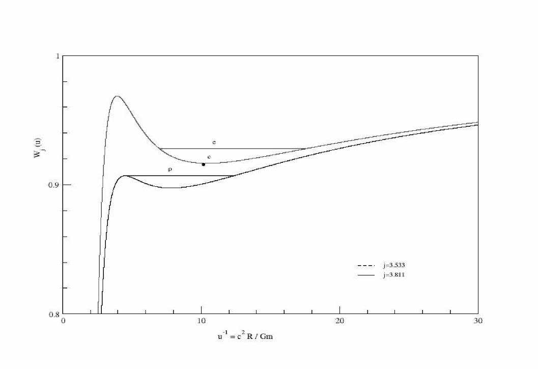
In the present paper, we study inspiralling eccentric orbits, evolving under radiation reaction, and we shall use a purely perturbative post-Newtonian approach (but one which goes beyond the zeroth order, adiabatic approximation). Such a treatment can only be valid if we stay sufficiently above any eccentric analog of the LSO, i.e. if we consider eccentric orbits which are ‘stable’ in the sense of being separated by a potential barrier from any plunge motion. The purpose of this section is to delineate, in the plane of the parameters representing the two-dimensional manifold of eccentric orbits, the locus where such orbits would cease to be bona fide bound orbits to become plunge-type ones. To do this, we need to use the non-perturbative effective one body (EOB) formalism, because the transition between bound and plunge orbits has a non-perturbative, strong-field origin. As the rest of the paper will consider the conservative part of the orbital motion at the second post-Newtonian (2PN) approximation, we shall consistently use the EOB Hamiltonian at the resummed 2PN level BD99 . (To work at the 3PN level one should use the more complicated EOB formalism derived in DJS00 ).

The real (resummed 2PN) EOB Hamiltonian describing the conservative part of the orbital motion (i.e. when neglecting radiation reaction), has the form (we recall that $\eta\equiv\mu/m\equiv m_{1}m_{2}/(m_{1}+m_{2})^{2}$)

$$H_{\rm real}(R,P_{R},P_{\phi})=mc^{2}\sqrt{1+2\eta\left(\widehat{H}_{\rm eff}-1\right)}\,,{\rm where},$$ (8)

$$\widehat{H}_{\rm eff}\equiv\frac{H_{\rm eff}}{\mu c^{2}}=\sqrt{A(R)\left[1+\frac{{\cal{J}}^{2}}{\mu^{2}c^{2}R^{2}}+\frac{P_{R}^{2}}{\mu^{2}c^{2}B(R)}\right]}\,,{\rm and},$$ (9)

$$A(R)=1-\frac{2Gm}{c^{2}R}+2\eta\left(\frac{Gm}{c^{2}R}\right)^{3}\,.$$ (10)

Here $R$ denotes the effective radial separation between the two bodies, $P_{R}$ the corresponding (relative) radial momentum, and ${\cal{J}}$ the (relative) total angular momentum. The total energy (including the rest mass) will be denoted by ${\cal E_{\rm real}}$ (or simply ${\cal E}$ when no confusion with the ‘effective’ energy can arise ). The total energy ${\cal E_{\rm real}}=H_{\rm real}$ is related to the ‘effective’ specific energy $\widehat{E}_{\rm eff}=\widehat{H}_{\rm eff}$ by ${\cal E}_{\rm real}=m\,c^{2}\,\sqrt{1+2\eta\left(\widehat{E}_{\rm eff}-1\right)}$. We shall not need the explicit expression of the EOB metric component $B(R)$, but only use the fact that $B(R)>0$. Taking into account the fact that the radial kinetic energy term $P_{R}^{2}/(\mu^{2}c^{2}B(R))$ in Eq. (9) is positive, the radial motion can be qualitatively understood in terms of the angular-momentum dependent (effective) ‘radial potential’

$$W_{{\cal{J}}}(R)\equiv A(R)\left[1+\frac{{\cal{J}}^{2}}{\mu^{2}c^{2}R^{2}}\right]\,,$$ (11)

which is a generalization (to the comparable mass case) of the well-known radial potential for test-particle orbits around a Schwarzschild black hole, namely,

$$W_{{\cal{J}}}^{0}(R)=(1-2Gm/c^{2}R)(1+{\cal{J}}^{2}/(\mu^{2}c^{2}R^{2}))$$ (12)

(which is simply the $\eta\rightarrow 0$ limit of Eq. (11)).

In Fig. 1, we present typical plots of $W_{{\cal{J}}}(R)$ on which we mark ‘energy levels’ corresponding to some eccentric and circular orbits. This plot makes it clear that an a priori bound motion (i.e. with total energy ${\cal{E}}_{\rm real}<mc^{2}$, i.e. $\widehat{E}_{\rm eff}<1$) will execute some precessing but stable motion only if the energy-level $\widehat{H}^{2}_{\rm eff}=\widehat{E}^{2}_{\rm eff}$ stays above the radial potential $W_{{\cal{J}}}(R)$ in a finite radial interval $\left[R_{\rm min}\,,\,R_{\rm max}\right]$. The ‘centrifugal barrier’ preventing this radial motion to plunge towards smaller separations is on the left of $R_{\rm min}$. Therefore the locus of orbits which are on the verge of plunging corresponds to the case where the energy-level (horizontal) line would be tangent to the top of the potential barrier, i.e. to

$$\frac{dW_{{\cal{J}}}(R)}{dR}=0\,.$$ (13)

In the domain of interest, the Eq. (13), considered for some given ${\cal{J}}$, will have two roots, say $R_{p}({\cal{J}})$ and $R_{c}({\cal{J}})$, with $R_{p}<R_{c}$. The larger root $R_{c}({\cal{J}})$ defines the set of stable circular orbits. Note, in this respect, that the smaller root $R_{p}({\cal{J}})$, which marks the ‘plunge’ locus also corresponds to the locus of unstable circular orbits. Finally, the domain in the energy-angular momentum plane corresponding to bound (non plunge) motion is restricted by the inequalities

$$W_{{\cal{J}}}(R_{c}({\cal{J}}))<\widehat{E}^{2}_{\rm eff}<W_{{\cal{J}}}(R_{p}({\cal{J}}))\,,$$ (14)

which defines, when using the link (8), a corresponding double inequality involving ${\cal{J}}$ and ${\cal{E}}_{\rm real}$. Note that, as one approaches the plunge boundary, i.e. for orbits close to the orbit marked ‘p’ in Fig. 1, the character of the orbital motion starts to deviate very much from that of a usual, perturbative, slowly precessing, “quasi-Keplerian” motion. Instead, it becomes what is referred to as a “zoom-whirl” motion in GK02 , i.e. a motion which alternates between one large-excursion elliptic-Keplerian-like orbit and several quasi-circular orbits near the periastron (which, as noted above is close to an unstable circular orbit). As the formalism we shall use in this paper to analytically represent the orbital motion assumes a “quasi-Keplerian” representation (see below), we shall need to stay sufficiently away from the plunge boundary to ensure the numerical validity of such a representation. Before coming to the issue of what one exactly means by “sufficiently away”, let us finish describing the analytical estimate of the plunge boundary, as defined by the inequalities given in Eq. (14).

Let us analytically estimate the two crucial roots $R_{p}({\cal{J}})$ and $R_{c}({\cal{J}})$ of Eq. (13). Using the dimensionless, scaled variables $u\equiv Gm/c^{2}R$, $j\equiv c{\cal{J}}/(\mu Gm)$, the radial potential reads

$$W(u) = A(u)\left(1+j^{2}u^{2}\right)\;$$ (15a)

$${\rm where},\;A(u) = 1-2u+2\eta u^{3}\,.$$ (15b)

The equation (13), or better $-W^{\prime}(u)/(2j^{2})$, reads

$$3u^{2}-u+\frac{1}{j^{2}}-\eta u^{2}(\frac{3}{j^{2}}+5u^{2})=0\,.$$ (16)

When $\eta\rightarrow 0$, Eq. (16) becomes a quadratic equation, with the two roots

$$u^{\pm}_{0}(j)\equiv\frac{1}{6}\left[1\pm\sqrt{1-\frac{12}{j^{2}}}\;\;\right]\,,$$ (17)

where the plus sign corresponds to the ‘plunge’ boundary (larger $u$, i.e. smaller $R$), while the minus sign corresponds to circular orbits. An accurate (at least when $j^{2}>12$) analytical estimate of the $\eta$-deformations of the above two roots, i.e. the roots of the quartic equation, Eq. (16), corresponding to $R_{p}$ and $R_{c}$, is obtained by inserting expressions (17) into the $\eta$-dependent terms in Eq. (16). This yields

$$u^{\pm}(j)\simeq\frac{1}{6}\left[1\pm\sqrt{1-\frac{12}{j^{2}}\left[1-\eta(u_{0}^{\pm})^{2}(3+5j^{2}(u_{0}^{\pm})^{2})\right]}\;\right]\,.$$ (18)

We have verified that the analytical estimate, Eq. (18), is a numerically accurate estimate of the two roots $u_{p}(j)$, $u_{c}(j)$. Inserting this result (with $u^{+}=u_{p}$, $u^{-}=u_{c}$) into Eq. (14) then yields an explicit (2PN-level) estimate of the domain of ‘non-plunge’ eccentric orbits in the $({\cal{E}},{\cal{J}})$ plane. Another way to describe the plunge boundary in the $({\cal{E}},{\cal{J}})$ plane, which does not need to assume that $j^{2}>12$, is to give a parametric representation of this boundary in terms of the parameter $u$ in the form ${\cal{E}}={\cal{E}}(u),{\cal{J}}={\cal{J}}(u)$. This is simply obtained by solving Eq. (16) for $j$, which gives $j(u)=\frac{\sqrt{1-3\,\eta\,u^{2}}}{\sqrt{u\,(1-3\,u+5\,\eta\,u^{3})}}$. One then obtains ${\cal{E}}={\cal{E}}(u)$ by substituting for ${\cal{J}}$ by $\frac{j(u)\,\mu\,G\,m}{c}$ in Eqs. (8) and (9).

Having discussed the location of the plunge boundary, let us now discuss the issue of ‘how far from the boundary’ we need to stay for allowing us to rightfully use the analytical quasi-Keplerian representation of DS88 ; SW93 (see Eqs. (26) below). As this representation assumes, among other things, that the orbits are slowly precessing, we need to set an upper limit on the rate of periastron precession. [This will then, de facto, eliminate the possibility of whirl-zoom orbits, which contain, during part of their orbital period, a rapidly precessing quasi-circular motion]. To see more precisely what upper limit we should set on periastron precession, let us go back to the EOB representation of the motion. From previous work on the 2PN-accurate EOB dynamics BD99 , we know that the comparable mass case ($\eta\sim 0.25$) is rather close to the test-mass one ($\eta\rightarrow 0$), yielding geodesic motion in a Schwarzschild spacetime. Therefore, let us consider the domain of parameter space for which periastron precession around a Schwarzschild black hole is well described by a slowly precessing, quasi-Keplerian motion. For this, we consider the exact formula, given by Eq. (A8) in the Appendix A of DS88 , which gives the angle of return to the periastron for a test particle moving in Schwarzschild spacetime. It can be easily checked that, for the elliptical orbits ( the eccentricity parameter $e_{t}<1$) we are interested in, the term whose expansion is most slowly convergent is the prefactor $(1-\frac{12}{j^{2}})^{-1/4}$ in Eq. (A8) of DS88 . We must therefore impose $\frac{12}{j^{2}}\ll 1$ to have a slowly precessing, quasi-Keplerian motion. When this inequality is satisfied (together with $0\leq e_{t}<1$), we expect that the 2PN-accurate expressions for $n=\frac{2\,\pi}{T}$, $T$ being the radial orbital period, and $e_{t}^{2}$ in terms of ${\cal{E}}$ and ${\cal{J}}$, as derived in DS88 ; SW93 , to be numerically accurate. In terms of dimensionless non-relativistic energy per unit reduced mass $E\equiv{({\cal E}-m\,c^{2})}/{\mu\,c^{2}}$ and $j$, defined earlier as $c{\cal{J}}/(\mu Gm)$, the expressions for $n$ and $e_{t}^{2}$ read E_def

$$\xi\equiv\frac{G\,m\,n}{c^{3}} = (-2\,E)^{3/2}\biggl{\{}1-\frac{1}{8}\left(15-\eta\right)(-2\,E)+\frac{(-2\,E)^{2}}{128}\left(555+30\,\eta+11\,\eta^{2}\right)$$ (19a)

$$-\frac{3}{2}\left(5-2\,\eta\right)\frac{(-2\,E)^{3/2}}{j}\biggr{\}}\,,$$

$$e_{t}^{2} = 1+2\,E\,j^{2}+{E}\biggl{\{}4\,(1-\eta)+(17-7\,\eta)\,E\,j^{2}\biggr{\}}+\biggl{\{}2(2+\eta+5\,\eta^{2})\,E^{2}$$ (19b)

$$-(17-11\,\eta)\frac{E}{j^{2}}+(112-47\,\eta+16\,\eta^{2})\,E^{3}j^{2}$$

$$-3(5-2\,\eta)(1+2\,Ej^{2})\frac{(-2\,E)^{3/2}}{j}\biggr{\}}\,.$$

Using the above expressions one can approximately express $\frac{12}{j^{2}}$ in terms of $\xi$ and $e_{t}$, and define

$$\epsilon\equiv\frac{12}{j^{2}}\sim 12\,\frac{\xi^{2/3}}{(1-e_{t}^{2})}$$ (20)

We can now specify ‘what small means’ in terms of $\epsilon$ to ensure a decent convergence of the crucial factor $(1-\epsilon)^{-1/4}$ entering the periastron precession expression. A minimal requirement would be to impose $\epsilon<\frac{1}{4}$. Indeed, when $\epsilon=\frac{1}{4}$ the 2PN-accurate expression for the periastron-advance parameter $k^{\prime}\equiv(1-\epsilon)^{-1/4}-1$, (which yields the periastron advance of nearly circular orbits) namely $k^{\prime}=\frac{\epsilon}{4}+\frac{5\,\epsilon^{2}}{32}$ gives the exact value to an accuracy $\sim 3\%$. Choosing such a threshold, $\epsilon<\frac{1}{4}$, for ‘staying sufficiently away from the plunge boundary’ leads to the following constraint on the parameters $\xi$ and $e_{t}$:

$$\frac{\xi}{(1-e_{t}^{2})^{3/2}}=\biggl{(}\frac{\epsilon}{12}\biggr{)}^{3/2}<3.0\times 10^{-3}$$ (21)

Later, when we evolve orbital elements and gravitational waveforms, we make sure that the eccentric orbits we study lie inside this domain, defined by the above inequality. Let us emphasize that this restriction is due to our use of, in the next section, the generalized quasi-Keplerian representation, given by Eqs. (28), (29) and (30). We could go beyond the limit, given by Eq. (21), by using, instead of the generalized quasi-Keplerian representation, the exact Schwarzschild-like motion (analytically expressible in terms of rather simple quadratures) in the EOB metric. This will be tackled in the near future.

IV A method of variation of constants

In this section, we introduce a version of the general Lagrange method of variation of arbitrary constants, which was employed to compute, within general relativity, the orbital evolution of the Hulse-Taylor binary pulsar TD83 ; TD_F85 . The method begins by splitting the relative acceleration of the compact binary ${\cal A}$ into two parts, an integrable leading part ${\cal A}_{0}$ and a perturbation part, ${\cal A}^{\prime}$ as

$$\mathbf{{\cal A}}=\mathbf{{\cal A}}_{0}+\mathbf{{\cal A}^{\prime}}\,.$$ (22)

In this work, we will work at 2.5PN accuracy and accordingly choose $\mathbf{{\cal A}}_{0}$ to be the acceleration at 2PN order and $\mathbf{{\cal A}}^{\prime}$ to be the $c^{-5}$ (leading) contribution to radiation reaction. It will, however, be clear that our method is general and can be applied, for instance, to a 3.5PN-accurate calculation where $\mathbf{{\cal A}}_{0}$ would be the conservative part of the 3PN dynamics, and $\mathbf{{\cal A}}^{\prime}$ the ${\cal{O}}(c^{-5})+{\cal{O}}(c^{-7})$ radiation reaction. The method first constructs the solution to the ‘unperturbed’ system, defined by

$$\dot{\mathbf{x}} = \mathbf{v}\,,$$ (23a)

$$\dot{\mathbf{v}} = {\cal A}_{0}(\mathbf{x},\mathbf{v}).$$ (23b)

The solution to the exact system

$$\dot{\mathbf{x}} = \mathbf{v}\,,$$ (24a)

$$\dot{\mathbf{v}} = {\cal A}(\mathbf{x},\mathbf{v})\,,$$ (24b)

is then obtained by varying the constants in the generic solutions of the unperturbed system, given by Eqs. (23). The method assumes (as is true for $\mathbf{{\cal A}}_{2PN}^{\rm conservative}$ or $\mathbf{{\cal A}}_{3PN}^{\rm conservative}$) that the unperturbed system admits sufficiently many integrals of motion to be integrable. For instance, if we work with $\mathbf{{\cal A}}_{0}=\mathbf{{\cal A}}_{2PN}$, we have four first integrals: the 2PN accurate energy and 2PN accurate angular momentum of the binary. We denote these quantities, written in the 2PN accurate center of mass frame as $c_{1}$ and $c_{2}^{i}$:

$$c_{1} = {\cal E}(\mathbf{x_{1}},\mathbf{x_{2}},\mathbf{v_{1}},\mathbf{v_{2}})|_{\rm 2PN~{}CM}\,,$$ (25a)

$$c_{2}^{i} = {\cal J}_{i}(\mathbf{x_{1}},\mathbf{x_{2}},\mathbf{v_{1}},\mathbf{v_{2}})|_{\rm 2PN~{}CM}\,,$$ (25b)

with corresponding 3PN definitions of $c_{1}$ and $c_{2}^{i}$, if we were working with $\mathbf{{\cal A}}_{0}=\mathbf{{\cal A}}_{3PN}^{\rm conservative}$.

The vectorial structure of $c_{2}^{i}$, indicates that the unperturbed motion takes place in a plane. The problem is restricted to a plane even in the presence of radiation reaction TD83 . We may therefore introduce polar coordinates in the plane of the orbit $r$ and $\phi$ such that $\mathbf{x}=\mathbf{i}\,r\cos\phi+\mathbf{j}\,r\sin\phi$ with, say, $\mathbf{i}=\mathbf{p}$, $\mathbf{j}=\mathbf{q}\cos i+\mathbf{N}\sin i$ (see above). The functional form for the solution to the unperturbed equations of motion, following TD83 ; DS88 , may be expressed as

$$r=S(l;c_{1},c_{2})\;\; \;\;\dot{r}=n\frac{\partial S}{\partial l}(l;c_{1},c_{2})\,,$$ ; (26a)

$$\phi=\lambda+W(l;c_{1},c_{2})\;\; \;\;\dot{\phi}=(1+k)n+n\frac{\partial W}{\partial l}(l;c_{1},c_{2})\,,$$ ; (26b)

where $\lambda$ and $l$ are two basic angles, which are $2\pi$ periodic and $c_{2}=|c_{2}^{i}|$. The functions $S(l)$ and $W(l)$ and therefore $\frac{\partial S}{\partial l}(l)$ and $\frac{\partial W}{\partial l}(l)$ are periodic in $l$ with a period of $2\pi$. In the above equations, $n$ denotes the unperturbed ‘mean motion’, given by $n=\frac{2\pi}{P},$ $P$ being the radial (periastron to periastron) period, while $k=\Delta\Phi/2\pi$, $\Delta\Phi$ being the advance of the periastron in the time interval $P$. The explicit 2PN accurate expressions for $P$ and $k$ in terms of $c_{1}$ and $c_{2}$ are given in DS88 . The corresponding 3PN accurate ones are given in DJS00B . The angles $l$ and $\lambda$ satisfy, still for the unperturbed system, $\dot{l}=n$ and $\dot{\lambda}=(1+k)n$, which integrate to

$$l = n(t-t_{0})+c_{l}\,,$$ (27a)

$$\lambda = (1+k)n(t-t_{0})+c_{\lambda}\,,$$ (27b)

where $t_{0}$ is some initial instant and the constants $c_{l}$ and $c_{\lambda}$, the corresponding values for $l$ and $\lambda$. Finally, the unperturbed solution depends on four integration constants: $c_{1}$, $c_{2}$, $c_{l}$ and $c_{\lambda}$.

At the 2PN order, one can write down explicit expressions for the functions $S(l)$ and $W(l)$. Indeed, the generalized quasi-Keplerian representation DS88 ; SW93 yields:

$$S(l;c_{1},c_{2}) = a_{r}(1-e_{r}\cos u)\,,$$ (28a)

$$W(l;c_{1},c_{2}) = (1+k)(v-l)+\frac{f_{\phi}}{c^{4}}\sin 2v+\frac{g_{\phi}}{c^{4}}\sin 3v\,,$$ (28b)

where $v$ and $u$ are some 2PN accurate true and eccentric anomalies, which must, in Eq. (28), be expressed as functions of $l,\,c_{1},\,$ and $c_{2}$, say as $v={\cal{V}}(l;c_{1},c_{2})=V({\cal{U}}(l;c_{1},c_{2}))$ and $u={\cal{U}}(l;c_{1},c_{2})$. In the above equations, $a_{r}$ and $e_{r}$ are some 2PN accurate semi-major axis and radial eccentricity, while $f_{\phi}$ and $g_{\phi}$ are certain functions, given in terms of $c_{1}$ and $c_{2}$. [To avoid introducing new notation, the eccentric anomaly is denoted by $u$ following standard convention. It should not be confused with $u=Gm/c^{2}R$ employed in Sec. III. A similar comment applies to the function $v$ below in the quasi-Keplerian representation and the magnitude of the relative velocity $v$.] The definitions of 2PN accurate functions $u={\cal{U}}(l;c_{1},c_{2})$ and $v=V(u)$ are available in DS88 ; SW93 . First, the function $v\equiv V(u)$ is defined by

$$v=V(u)\equiv 2\arctan{\biggl{(}\biggl{(}\frac{1+e_{\phi}}{1-e_{\phi}}\biggr{)}^{1/2}\tan\frac{u}{2}\biggr{)}}\,.$$ (29)

Second, the function $u={\cal{U}}(l)$ is defined by inverting the following ‘Kepler equation’ $l=l(u)$

$$l=u-e_{t}\sin u+\frac{f_{t}}{c^{4}}\sin V(u)+\frac{g_{t}}{c^{4}}(V(u)-u)\,.$$ (30)

Then the function $v={\cal{V}}(l)$ is obtained by inserting $u={\cal{U}}(l)$ in $v=V(u)$, i.e. ${\cal{V}}(l)\equiv V({\cal{U}}(l))$. Here $e_{t}$ and $e_{\phi}$ are some time and angular eccentricity and $f_{t}$ and $g_{t}$ are certain functions of $c_{1}$ and $c_{2}$, appearing at the 2PN order. In our computations, we use the following exact relation for $v-u$, which is also periodic in $u$, given by

$$v-u=2\,\tan^{-1}\biggl{(}\frac{\beta_{\phi}\,\sin u}{1-\beta_{\phi}\,\cos u}\biggr{)}\,,$$ (31)

where $\beta_{\phi}=\frac{1-\sqrt{1-e_{\phi}^{2}}}{e_{\phi}}$. We note that the extension of such a generalized quasi-Keplerian representation to the 3PN order is easily possible when working in ADM type coordinates.

Let us now turn to use the explicit unperturbed solution, Eqs. (26) and (27), for the construction of the general solution of the perturbed system, Eqs. (24). This is done by keeping exactly the same functional form for $r$, $\dot{r}$, $\phi$ and $\dot{\phi}$, as functions of $l$ and $\lambda$, Eqs. (26), i.e. by writing

$$r=S(l;c_{1},c_{2})\;\; \;\;\dot{r}=n\frac{\partial S}{\partial l}(l;c_{1},c_{2})\,,$$ ; (32a)

$$\phi=\lambda+W(l;c_{1},c_{2})\;\; \;\;\dot{\phi}=(1+k)n+n\frac{\partial W}{\partial l}(l;c_{1},c_{2}),$$ ; (32b)

but by allowing temporal variation in $c_{1}=c_{1}(t)$ and $c_{2}=c_{2}(t)$ [with corresponding temporal variation in $n=n(c_{1},c_{2})$ and $k=k(c_{1},c_{2})$], and, by modifying the unperturbed expressions, given by Eqs. (27), for the temporal variation of the basic angles $l$ and $\lambda$ entering Eqs. (32) into the new expressions:

$$l \equiv \int_{t_{0}}^{t}n\,dt\,+\,c_{l}(t)\,,$$ (33a)

$$\lambda \equiv \int_{t_{0}}^{t}(1+k)\,n\,dt\,+\,c_{\lambda}(t)\,,$$ (33b)

involving two new evolving quantities $c_{l}(t)$, and $c_{\lambda}(t)$. In other words, we seek for solutions of the exact system, Eqs. (24), in the form given by Eqs. (32) and (33) with four ‘varying constants’ $c_{1}(t)$, $c_{2}(t)$, $c_{l}(t)$ and $c_{\lambda}(t)$. The four variables $\{c_{1},c_{2},c_{l},c_{\lambda}\}$ replace the original four dynamical variables $r$, $\dot{r}$, $\phi$ and $\dot{\phi}$. It can be verified that the alternate set $\{c_{1}$, $c_{2}$, $c_{l},c_{\lambda}\}$ satisfies, like the original phase-space variables, first order evolution equations TD83 ; TD_F85 . These evolution equations have a rather simple functional form, namely,

$$\frac{dc_{\alpha}}{dt}=F_{\alpha}(l;c_{\beta})\;;\,\alpha,\beta=1,2,l,\lambda\,,$$ (34)

where the right hand side is linear in the perturbing acceleration, ${\cal A}^{\prime}$. Note the presence of the sole angle $l$ (apart from the implicit time dependence of $c_{\beta}$) on the RHS of Eqs. (34). The explicit expressions for these evolution equations were derived in TD_F85 , which in our notation read

$$\frac{dc_{1}}{dt} = \frac{\partial c_{1}(\mathbf{x},\mathbf{v})}{\partial v^{i}}\,{\cal A^{\prime}}^{i}\,,$$ (35a)

$$\frac{dc_{2}}{dt} = \frac{\partial c_{2}(\mathbf{x},\mathbf{v})}{\partial v^{j}}\,{\cal A^{\prime}}^{j}\,,$$ (35b)

$$\frac{dc_{l}}{dt} = -\biggl{(}\frac{\partial S}{\partial l}\biggr{)}^{-1}\biggl{(}\frac{\partial S}{\partial c_{1}}\,\frac{dc_{1}}{dt}+\frac{\partial S}{\partial c_{2}}\,\frac{dc_{2}}{dt}\biggr{)}\,,$$ (35c)

$${dc_{\lambda}\over dt} = -\frac{\partial W}{\partial l}{dc_{l}\over dt}-\frac{\partial W}{\partial c_{1}}{dc_{1}\over dt}-\frac{\partial W}{\partial c_{2}}{dc_{2}\over dt}\,.$$ (35d)

The evolution equations for $c_{1}$ and $c_{2}$ clearly arise from the fact that $c_{1}$ and $c_{2}$ were defined as some first integrals in phase-space, say Eqs. (25). As shown in TD_F85 , there is an alternative expression for $\frac{dc_{l}}{dt}$, which reads

$$\frac{dc_{l}}{dt}=\biggl{(}\frac{\partial Q}{\partial l}\biggr{)}^{-1}\biggl{(}{\cal A^{\prime}}\cdot{\bf n}-\frac{\partial Q}{\partial c_{1}}\,\frac{dc_{1}}{dt}-\frac{\partial Q}{\partial c_{2}}\,\frac{dc_{2}}{dt}\biggr{)}\,,$$ (36)

where $Q^{2}(l,c_{1},c_{2})=\dot{r}^{2}(S(l,c_{1},c_{2}),c_{1},c_{2})$ and $\frac{\partial Q}{\partial l}$ is defined by

$$\frac{\partial Q}{\partial l}=\frac{P}{4\,\pi}\frac{\partial Q^{2}}{\partial r}\,.$$ (37)

Both expressions, Eqs. (35c) and (36), involve formal delicate limits of the $0/0$ form, for some (different) values of $l$. Taken together, they prove that these limits are well-defined and yield for $dc_{l}/dt$, an everywhere regular function of $l$. Anyway, the algebraic manipulation of the explicit forms of both Eqs. (35c) and (36) lead to well-defined expressions [For example, in the case of Eq. (35c), the problematic $\sin u$ factor in $\partial S/\partial l$, see Eq. (48a) below, nicely simplifies with a $\sin u$ factor present in the term within parenthesis on the RHS of Eq. (35c)].

The definition of $l$ given by $l=\int_{t_{0}}^{t}n(c_{a}(t))\,dt\,+\,c_{l}(t)$, is equivalent to the differential form, $\frac{dl}{dt}=n+\frac{dc_{l}}{dt}=n+F_{l}(l,c_{a});a=1\,,\,2$, which allow us to define a set of differential equations for $c_{\alpha}$ as functions of $l$ similar to Eqs. (34) for $c_{\alpha}$ as functions of $t$. The exact form of the differential equations for $c_{\alpha}(l)$ reads

$$\frac{dc_{\alpha}}{dl}=\frac{F_{\alpha}(l;c_{a})}{n(c_{a})+F_{l}(l;c_{a})},$$ (38)

where $c_{a}$, $a=1,2,$ stands for $c_{1}$ and $c_{2}$. Neglecting terms quadratic in $F_{\alpha}$, i.e. quadratic in the perturbation $\mathbf{{\cal{A}}}^{\prime}$ (e.g. neglecting ${\cal{O}}(c^{-10})$ terms in our application), we can simplify the system above to

$$\frac{dc_{\alpha}}{dl}\simeq\frac{1}{n(c_{a})}\,F_{\alpha}(l;c_{a})\equiv G_{\alpha}(l;c_{a})\;;\,\alpha=1,2,l,\lambda\,;a=1\,,\,2\,.$$ (39)

From here onward, we will neglect these ${\cal{O}}(c^{-10})$ terms in the evolution equations for $c_{\alpha}(l)$, i.e. work with the simplified system, namely Eq. (39). At this stage, it is crucial to note, not only that the RHS of Eq. (39) is a function of $c_{1}$, $c_{2}$ and the sole angle $l$ (and not of $\lambda$), but that it is a periodic function of $l$. This periodicity, together with the slow [$G_{\alpha}\propto F_{\alpha}\propto\mathbf{{\cal{A}}}^{\prime}={\cal{O}}(c^{-5})$] evolution of the $c_{\alpha}$’s, implies that the evolution of $c_{\alpha}(l)$ contains both a ‘slow’ (radiation-reaction time-scale) secular drift and ‘fast’ (orbital time-scale) periodic oscillations. For the purpose of phasing, to model the combination of slow drift and the fast oscillations present in $c_{\alpha}$, we introduce a two-scale decomposition for $c_{\alpha}(l)$ in the following manner

$$c_{\alpha}(l)=\bar{c}_{\alpha}(l)+\tilde{c}_{\alpha}(l)\,,$$ (40)

where the first term $\bar{c}_{\alpha}(l)$ represents a slow drift (which can ultimately lead to large changes in the ‘constants’ $c_{\alpha}$) and $\tilde{c}_{\alpha}(l)$ represents fast oscillations (which will stay always small, i.e. of order ${\cal{O}}(G_{\alpha})={\cal{O}}(c^{-5})$). This is proved by first decomposing the periodic functions $G_{\alpha}(l)$ (considered for fixed values of the other arguments $c_{a}$ ) into its average part and its oscillatory part:

$$\bar{G}_{\alpha}(c_{a}) \equiv \frac{1}{2\pi}\int_{0}^{2\pi}\,dl\,G(l,c_{a})\,,$$ (41a)

$$\tilde{G}_{\alpha}(l;c_{a}) \equiv G_{\alpha}(l;c_{a})-\bar{G}_{\alpha}(c_{a}).$$ (41b)

Note that, by definition, the oscillatory part $\tilde{G}_{\alpha}(l)$ is a periodic function with zero average over $l$. Then assuming that $\tilde{c}_{\alpha}$ in Eq. (40) is always small ($\tilde{c}_{\alpha}={\cal{O}}(G_{\alpha})={\cal{O}}(c^{-5})$), one can expand the RHS of the exact evolution system, given by Eqs. (39), as

$$\frac{d\bar{c}_{\alpha}}{dl}+\frac{d\tilde{c}_{\alpha}}{dl} = G_{\alpha}(l;\bar{c}_{a}+\tilde{c}_{a})=G_{\alpha}(l;\bar{c}_{a})+{\cal{O}}(G_{\alpha}^{2})\,,$$ (42)

$$= \bar{G}_{\alpha}(l;\bar{c}_{a})+\tilde{G}_{\alpha}(l;\bar{c}_{a})+{\cal{O}}(G_{\alpha}^{2})\,.$$

We can then solve, modulo ${\cal{O}}(G_{\alpha}^{2})$, the evolution equation (42) by defining $\bar{c}_{\alpha}(l)$ as a solution of the ‘averaged system’

$$\frac{d\bar{c}_{\alpha}}{dl}=\bar{G}_{\alpha}(\bar{c}_{a})\,,$$ (43)

and by defining $\tilde{c}_{\alpha}(l)$ as a solution of the ‘oscillatory part’ of the system

$$\frac{d\tilde{c}_{\alpha}}{dl}=\tilde{G}_{\alpha}(l,\bar{c}_{a})\,.$$ (44)

During one orbital period ($0\leq l\leq 2\pi$) the quantities $\bar{c}_{a}$ on the RHS of Eq. (44) change only by ${\cal{O}}(G_{\alpha})$. Therefore, by neglecting again terms of order ${\cal{O}}(G_{\alpha}^{2})\sim{\cal{O}}(c^{-10})$ in the evolution of $\tilde{c}_{\alpha}$, we can further define $\tilde{c}_{\alpha}(l)$ as the unique zero-average solution of Eq. (44), considered for fixed values of $\bar{c}_{a}$, i.e.

$$\tilde{c}_{\alpha}(l)=\int dl\,\tilde{G}_{\alpha}(l;\bar{c}_{a})|_{\bar{c}_{a}=\bar{c}_{a}(l)}=\int\frac{dl}{n}\,\tilde{F}_{\alpha}(l;\bar{c}_{a})\,.$$ (45)

The indefinite integral in Eq. (45) is defined as the unique zero-average periodic primitive of the zero-average (periodic) function $\tilde{G}_{\alpha}(l)$. During that integration, the arguments $\bar{c}_{a}$ are kept fixed, and, after the integration, they are replaced by the slowly drifting solution of the averaged system, given by Eqs. (43). Note that Eq. (44) yields $\tilde{c}_{\alpha}={\cal{O}}(G_{\alpha})$, which was assumed above, thereby verifying the consistency of the (approximate) two-scale integration method used here.

We are now in a position to apply the above described method of variation of arbitrary constants, which gave us the evolution equations for $\bar{c}_{\alpha}$ and $\tilde{c}_{\alpha}$, to GW phasing. We use 2PN accurate expressions for the dynamical variables $r$, $\dot{r}$, $\phi$ and $\dot{\phi}$ entering the expressions for $h_{\times}$ and $h_{+}$, given by Eqs. (6). To do the phasing, we will solve the evolution equations for $\{c_{1},c_{2},c_{l},c_{\lambda}\}$, given by Eqs. (39), on the 2PN accurate orbital dynamics, given in Eqs. (26). This leads to an evolution system, given by Eqs. (43) and (44), in which the RHS contains terms of order ${\cal{O}}(c^{-5})\times\left[1+{\cal{O}}(c^{-2})+{\cal{O}}(c^{-4})\right]={\cal{O}}(c^{-5})+{\cal{O}}(c^{-7})+{\cal{O}}(c^{-9})$. In the next section, as a first step, we will restrict our attention to the leading order contributions to $\bar{G}_{\alpha}$ and $\tilde{G}_{\alpha}$, which define the evolution of $\{\bar{c}_{\alpha},\tilde{c}_{\alpha}\}$ under gravitational radiation reaction to ${\cal{O}}(c^{-5})$ order. We then impose these variations, via Eqs. (32) and (33), on to $h_{\times}$ and $h_{+}$, given by Eqs. (6). This will allow us to obtain gravitational wave polarizations, which are Newtonian accurate in their amplitudes and 2.5PN accurate in orbital dynamics. We name the above procedure 2.5PN accurate phasing of gravitational waves. Since $\tilde{G}_{\alpha}$’s create only periodic 2.5PN corrections to the dynamics, in this paper, we will not explore its higher PN corrections. However, in a later section, we will present the consequences of considering PN corrections to $\bar{G}_{\alpha}$ by computing ${\cal{O}}(c^{-9})$ contributions to relevant $\frac{d\bar{c}_{\alpha}}{dt}$. This is required as $\bar{G}_{\alpha}$ directly contribute to the highly important adiabatic evolution of $h_{\times}$ and $h_{+}$.

Up to now we have assumed, for concreteness, that the two constants $c_{1}$ and $c_{2}$ were the energy and the angular momentum, respectively. However, any functions of these conserved quantities can do as well. In view of our use of the generalized quasi-Keplerian representation to describe the orbital dynamics, it is convenient to follow GI02 and to use as $c_{1}$ the mean motion $n$, and as $c_{2}$ the time-eccentricity $e_{t}$. This can be done by employing the 2PN accurate expressions for $n$ and $e_{t}$ in terms of ${\cal E}$ and ${\cal J}$ (or rather E and j), derived in DS88 ; SW93 . Firstly, this will require us to express 2PN accurate orbital dynamics in terms of $l,n$ and $e_{t}$. Secondly, using $n$ and $e_{t}$, instead of ${\cal{E}}$ and ${\cal{J}}$, as $c_{1}$ and $c_{2}$, we need to derive the evolution equations for $\frac{dn}{dt}$, $\frac{de_{t}}{dt}$,$\frac{dc_{l}}{dt}$ and $\frac{dc_{\lambda}}{dt}$ in terms of $l,n$ and $e_{t}$. This will follow straightforwardly from Eqs. (35). Using these expressions, the evolution equations, namely Eqs. (43) and (44), for $\{\bar{n},\bar{e}_{t},\bar{c}_{l},\bar{c}_{\lambda},\tilde{n},\tilde{e}_{t},\tilde{c}_{l},\tilde{c}_{\lambda}\}$ will be obtained in terms of $l,n$ and $e_{t}$.

As mentioned earlier, we restrict in this paper the conservative dynamics to the 2PN order. Below, we present the 2PN accurate orbital dynamics, given by Eqs. (32), explicitly in terms of $(l,n,e_{t})$. This straightforward computation employs explicit expressions for the orbital elements of generalized quasi-Keplerian representation, in terms of $E$ and $j$ available in DS88 ; SW93 . The relations we need are:

$$a_{r}(n,e_{t}) = \biggl{(}\frac{G\,m}{n^{2}}\biggr{)}^{1/3}\biggl{\{}1-\frac{\xi^{2/3}}{3}(9-\eta)+\frac{\xi^{4/3}}{72}\,\biggl{[}(72+75\,\eta+8\,\eta^{2}$$ (46a)

$$-\frac{1}{(1-e_{t}^{2})^{1/2}}(360-144\,\eta)-\frac{1}{(1-e_{t}^{2})}(306-198\,\eta)\biggr{]}\biggr{\}}\,,$$

$$e_{r}(n,e_{t}) = e_{{t}}\biggl{\{}1+{\xi^{2/3}\over 2}\,\left(8-3\,\eta\right)+{\xi^{4/3}\over 24\,(1-e_{t}^{2})^{3/2}}\,\biggl{[}\biggl{(}-(288-242\,\eta+21\,{\eta}^{2}){e_{{t}}}^{2}$$ (46b)

$$+390-308\,\eta+21\,{\eta}^{2}\biggr{)}\,\sqrt{1-e_{t}^{2}}+\left(180-72\,\eta\right)\,(1-e_{t}^{2})\biggr{]}\biggr{\}}\,,$$

$$e_{\phi}(n,e_{t}) = e_{{t}}\biggl{\{}1+{\xi}^{2/3}\left(4-\eta\right)+{\xi^{4/3}\over 96\,(1-e_{t}^{2})^{3/2}}\,\biggl{[}\biggl{(}-(1152-656\,\eta+41\,{\eta}^{2}){e_{{t}}}^{2}$$ (46c)

$$+1968-1088\,\eta-4\,{\eta}^{2}\biggr{)}\sqrt{1-e_{t}^{2}}+\left(720-288\,\eta\right)\,(1-e_{t}^{2})\biggr{]}\biggr{\}}\,,$$

$$k(n,e_{t}) = {3\,\xi^{2/3}\over(1-e_{t}^{2})}+{\xi^{4/3}\over 4\,(1-e_{t}^{2})^{2}}\biggl{\{}(51-26\,\eta)\,e_{t}^{2}+(78-28\,\eta)\biggr{\}}\,,$$ (46d)

$$f_{t}(n,e_{t}) = -\frac{\xi^{4/3}c^{4}}{8\,\sqrt{1-e_{t}^{2}}}(4+\eta)\,\eta\,e_{t}\,,$$ (46e)

$$g_{t}(n,e_{t}) = \frac{3\,\xi^{4/3}c^{4}}{2\,\sqrt{1-e_{t}^{2}}}(5-2\,\eta)\,,$$ (46f)

$$f_{\phi}(n,e_{t}) = \frac{\xi^{4/3}c^{4}}{8\,(1-e_{t}^{2})^{2}}(1-3\,\eta)\,\eta\,e_{t}^{2}\,,$$ (46g)

$$g_{\phi}(n,e_{t}) = -\frac{3\,\xi^{4/3}c^{4}}{32\,(1-e_{t}^{2})^{2}}\,\eta^{2}\,e_{t}^{3}\,,$$ (46h)

where $\xi\equiv\frac{Gmn}{c^{3}}$. We note that the generalized quasi-Keplerian orbital elements, given in terms of $E$ and $j$ in DS88 ; SW93 ; E_def , can easily be expressed in $n$ and $e_{t}$ using following 2PN accurate relations for $-2\,E$ and $-2\,E\,j^{2}$, which read

$${-2\,E} = {\xi}^{2/3}\biggl{\{}1+{{\xi}^{2/3}\over 12}\biggl{[}15-\eta\biggr{]}+{{\xi}^{4/3}\over 24\,}\biggl{[}\biggl{(}15-15\,\eta-\eta^{2}\biggr{)}$$ (47a)

$$+{1\over\sqrt{1-e_{t}^{2}}}\,\biggl{(}120-48\,\eta\biggr{)}\biggr{]}\biggr{\}}\,,$$

$$-2\,E\,j^{2} = (1-e_{t}^{2})\,\biggl{\{}1+{{\xi}^{2/3}\over 4\,(1-e_{t}^{2})}\biggl{[}-\left(17-7\,\eta\right){{e_{t}}}^{2}+9+\eta\biggr{]}$$ (47b)

$$+{{\xi}^{4/3}\over 24\,(1-e_{t}^{2})^{2}}\biggl{[}-\left(360-144\,\eta\right){{e_{t}}}^{2}\sqrt{1-e_{t}^{2}}+\left(225-277\,\eta+29\,{\eta}^{2}\right){{e_{t}}}^{4}$$

$$-\left(210-190\,\eta+30\,{\eta}^{2}\right){{e_{t}}}^{2}+189-45\,\eta+{\eta}^{2}\biggr{]}\biggr{\}}\,.$$

These two relations easily follow from inverting the 2PN accurate relations for the orbital period $P=\frac{2\,\pi}{n}$ and $e_{t}^{2}$ in terms of $E$ and $j$ presented in Eqs. (19) above [ See DS88 ; SW93 ].

In addition, to compute expressions for $\dot{r}$ and $\dot{\phi}$, we use the following relations

$$\frac{\partial S}{\partial l} = a_{r}\,e_{r}\,\sin u\,\frac{\partial u}{\partial l}\,,$$ (48a)

$$\frac{\partial W}{\partial l} = \left[\left(1+k+\frac{2f_{\phi}}{c^{4}}\cos 2v+\frac{3g_{\phi}}{c^{4}}\cos 3v\right)\frac{\partial v}{\partial u}\frac{\partial u}{\partial l}-\left(1+k\right)\right]\,,$$ (48b)

$$\frac{\partial u}{\partial l} = \biggl{(}1-e_{t}\cos u-\frac{g_{t}}{c^{4}}+\frac{1}{c^{4}}\left(f_{t}\cos v+g_{t}\right)\frac{\partial v}{\partial u}\biggr{)}^{-1}\,,$$ (48c)

$$\frac{\partial v}{\partial u} = \frac{(1-e_{\phi}^{2})^{1/2}}{1-e_{\phi}\cos u}\,.$$ (48d)

The radial motion, defined by $r(l,n,e_{t})$ and $\dot{r}(l,n,e_{t})$, reads (both in the compact form and in 2PN-expanded form)

$$r = S(l,n,e_{t})=a_{r}(n,e_{t})(1-e_{r}(n,e_{t})\cos u)$$ (49a)

$$=({G\,m\over n^{2}})^{1/3}\,(1-e_{t}\,\cos u)\,\biggl{\{}1-{{\xi}^{2/3}\over 6\,(1-e_{t}\,\cos u)}\biggl{[}\left(6-7\,\eta\right){e_{t}}\,\cos u+18-2\,\eta\biggr{]}$$

$$+{{\xi}^{4/3}\over 72\,\sqrt{(1-e_{t}^{2})^{3}}\,(1-e_{t}\,\cos u)}\biggl{[}\biggl{(}-(72-231\,\eta+35\,{\eta}^{2})(1-{{e_{t}}}^{2})\,e_{t}\,\cos u$$

$$-(72+75\,\eta+8\,{\eta}^{2}){{e_{t}}}^{2}-234+273\,\eta+8\,{\eta}^{2}\biggr{)}\,\sqrt{1-e_{t}^{2}}$$

$$-36\,(1-e_{t}^{2})\,(5-2\,\eta)\,(2+e_{t}\,\cos u)\biggr{]}\biggr{\}}\,,$$

$${\dot{r}} = n\frac{\partial S}{\partial l}(l,n,e_{t})={{(G\,m\,n)}^{1\over 3}\,\over{(1-e_{t}\,\cos u)}}\,{{e_{t}}\,\sin u}\biggl{\{}1+{{\xi}^{2/3}\over 6}\left(6-7\,\eta\right)$$ (49b)

$$+{\xi^{4/3}\over 72}\,{1\over(1-e_{t}\,\cos u)^{3}}\biggl{[}\biggl{(}-\left(72-231\,\eta+35\,{\eta}^{2}\right)\,(e_{t}\,\cos u)^{3}$$

$$+\left(216-693\,\eta+105\,{\eta}^{2}\right)\,(e_{t}\,\cos u)^{2}+\left(324+513\,\eta-96\,{\eta}^{2}\right)\,{e_{t}}\,\cos u$$

$$-\left(36+9\,{\eta}\right)\,\eta\,{{e_{t}}}^{2}-468-15\,\eta+35\,{\eta}^{2}\biggr{)}$$

$$+{36\over\sqrt{1-e_{t}^{2}}}\,\biggl{(}\left(1-{e_{t}}\,\cos u\right)^{2}\left(4-{e_{t}}\,\cos u\right)\left(5-2\,\eta\right)\biggr{)}\biggr{]}\biggr{\}}\,.$$

In the above equation, the eccentric anomaly $u={\cal U}(l,n,e_{t})$ is given by inverting the 2PN accurate Kepler equation, Eq. (30), connecting $l$ and $u$, i.e. in explicit form

$${l} = u-{e_{t}}\,\sin u-{{\xi}^{4/3}\over 8\,\sqrt{1-e_{t}^{2}}}\,{1\over(1-e_{t}\,\cos u)}\,\biggl{\{}e_{t}\,\sin u\,\sqrt{1-e_{t}^{2}}\,\eta\,\left(4+\eta\right)$$ (50)

$$+12\,(5-2\,\eta)\,(u-v)\left(1-e_{t}\,\cos u\right)\biggr{\}}\,.$$

The angular motion, described in terms of $\phi$ and $\dot{\phi}$, is given by

$$\phi(\lambda,l) = \lambda+W(l)$$ (51a)

$$W(l) = v-u+{e_{t}}\,\sin u+{3\,{\xi}^{2/3}\over(1-e_{t}^{2})}\biggl{\{}v-u+e_{t}\,\sin u\biggr{\}}$$ (51b)

$$+{\xi^{4/3}\over 32\,(1-e_{t}^{2})^{5/2}}\,{1\over(1-e_{t}\,\cos u)^{3}}\,\biggl{\{}\biggl{[}4\,\sqrt{1-e_{t}^{2}}\,\left(1-e_{t}\,\cos u\right)^{2}\biggl{(}\biggl{\{}-(102$$

$$-52\,\eta){{e_{t}}}^{2}-156+56\,\eta\biggr{\}}\,e_{t}\,\cos u+\eta\,\left(4+\eta\right){{e_{t}}}^{4}+\left(102-60\,\eta-2\,{\eta}^{2}\right){{e_{t}}}^{2}$$

$$+156-52\,\eta+{\eta}^{2}\biggr{)}+\left(1-e_{t}^{2}\right)\,\biggl{(}\left((3\,e_{t}^{2}+12)\,\eta-8\right){(e_{t}\,\cos u)}^{2}$$

$$+\left(\left(8-6\,\eta\right){e_{t}}^{2}+8-24\,\eta\right)(e_{t}\,\cos u)-12\,\eta\,{e_{t}}^{4}-\left(8-27\,\eta\right){e_{t}}^{2}\biggr{)}$$

$$\,\eta\biggr{]}\,e_{t}\,\sin u+(1-e_{t}\,\cos u)^{3}\,\biggl{[}48\,{(1-e_{t}^{2})}^{2}\left(5-2\,\eta\right)-8\,\biggl{(}(51-26\,\eta){e_{t}}^{2}$$

$$+78-28\,\eta\biggr{)}\biggr{]}\,u+8\,\left(1-{e_{t}}\,\cos u\right)^{3}\,\biggl{[}\biggl{(}\left(51-26\,\eta\right){{e_{t}}}^{2}$$

$$+78-28\,\eta\biggr{)}\,\sqrt{1-e_{t}^{2}}-(30-12\,\eta)\,(1-2\,e_{t}^{2}+e_{t}^{4})\biggr{]}\,v\biggl{\}}\,,$$

$${\dot{\phi}} = {n\,\sqrt{1-e_{t}^{2}}\over\left(1-{e_{t}}\,\cos u\right)^{2}}\biggl{\{}1+{\xi^{2/3}\over(1-e_{t}^{2})\,(1-e_{t}\,\cos u)}\biggl{[}\left(1-\eta\right){e_{t}}\,\cos u$$ (52)

$$-\left(4-\eta\right){{e_{t}}}^{2}+3\biggr{]}+{{\xi}^{4/3}\over 12}\,{1\over(1-e_{t}\,\cos u)^{3}}\biggl{[}{1\over(1-e_{t}^{2})^{3/2}}\biggl{\{}18\,\left(1-{e_{t}}\,\cos u\right)^{2}\,$$

$$\left({e_{t}}\,\cos u-2\,{{e_{t}}}^{2}+1\right)\left(5-2\,\eta\right)\biggr{\}}+{1\over{(1-e_{t}^{2})}^{2}}\biggl{\{}\biggl{(}-(9-19\,\eta-14\,{\eta}^{2}){{e_{t}}}^{2}$$

$$-36+2\,\eta-8\,{\eta}^{2}\biggr{)}\,(e_{t}\,\cos u)^{3}+\biggl{(}-(48-14\,\eta+17\,{\eta}^{2}){{e_{t}}}^{4}$$

$$+\left(69-79\,\eta+4\,{\eta}^{2}\right){{e_{t}}}^{2}+114+2\,\eta-5\,{\eta}^{2}\biggr{)}\,(e_{t}\,\cos u)^{2}$$

$$+\biggl{(}-(6-32\,\eta-{\eta}^{2}){{e_{t}}}^{4}+\left(93-19\,\eta+16\,{\eta}^{2}\right)e_{t}^{2}$$

$$-222+50\,\eta+{\eta}^{2}\biggr{)}\,(e_{t}\,\cos u)-6\,\eta\,(1-2\,\eta)\,e_{t}^{6}$$

$$+\left(54-28\,\eta-20\,{\eta}^{2}\right){{e_{t}}}^{4}-\left(153-61\,\eta-2\,{\eta}^{2}\right){{e_{t}}}^{2}+144-48\,\eta\biggr{\}}\biggr{]}\biggr{\}}\,.$$

The explicit form of $\dot{\phi}$ above follows from Eq. (32b).

In addition to the above explicit expressions, we also need to evaluate the RHS of Eqs. (35a)-(35b) and, in particular, the 2PN accurate partial derivatives of $n$ and $e_{t}$ with respect to the relative velocity ${\bf v}$. To get these, one could combine Eqs. (19) with the expressions for $E$ and $j$ in terms of relative position and velocity, rather than in terms of position and momenta as is usual in the ADM formalism. To the desired 2PN order, one may either start from the ordinary Lagrangian $L({\bf x},{\bf v})$ in ADM coordinates ( See DS85 for the explicit construction of this Lagrangian ) or (simply) by inverting the basic Hamiltonian equation ${\bf v}=dH/d{\bf p}$, to get ${\bf v}$ in terms of ${\bf p}$. However, in the next section, we require expressions for $E$ and $j$ only to the well known Newtonian order.

V 2.5PN accurate phasing

Let us recall that our method is general and can be applied, in principle, to any PN accuracy. For instance, we could study the effect of the ${\cal{O}}(c^{-5})+{\cal{O}}(c^{-7})$ radiation reaction on the 3PN conservative motion. However, in this work, we limit ourselves, for simplicity, to considering the effect of the ${\cal{O}}(c^{-5})$ radiation reaction on the 2PN motion. Accordingly, we shall, each time it is possible, truncate away all effects that would correspond to the ${\cal{O}}(c^{-7})$ level or beyond. As we shall see, this approximation is probably sufficient for oscillatory effects (in the sense of the decomposition, given in Eq. (40) ), which are the primary focus of this paper. We shall discuss below, how our method also justifies the usual way of deriving the secular effects linked to the radiation reaction, and we shall obtain more accurate expressions for them.

This section begins by providing inputs necessary for computing evolution equations for the set $\{{\bar{c}_{\alpha},\tilde{c}_{\alpha}}\}$, to the 2.5PN order, where the index $\alpha=n,e_{t},c_{l},$ and $c_{\lambda}$. As just said, we require ${\cal A^{\prime}}$ to 2.5PN order for this purpose. The 2.5PN expressions for ${\cal A^{\prime}}$ will have to be in the ADM gauge, as our conservative 2PN dynamics is given in the same gauge. The expression for relative reactive acceleration, to 2.5PN order, in the ADM gauge, available in GS85 , reads

$${\cal A^{\prime}}^{i}=-\frac{8\,G^{2}\,m^{2}\,\eta}{15\,c^{5}\,r^{3}}\biggl{\{}-3\biggl{[}12\,v^{2}-15\,\dot{r}^{2}+2\,\frac{G\,m}{r}\biggr{]}\dot{r}\,n^{i}+\biggl{[}11\,v^{2}-24\,\dot{r}^{2}+\frac{G\,m}{r}\biggr{]}\,v^{i}\biggr{\}}\,,$$ (53)

where $v^{2}=\dot{r}^{2}+r^{2}\,\dot{\phi}^{2}$. At this point a nice technical simplification occurs. Though our formalism consistently combines a 2PN-accurate, precessing motion with 2.5PN radiation reaction, the RHS’s of Eqs. (39) are technically given by the product of ${\cal{O}}(c^{-5})$ reaction terms by orbital expressions given as explicit PN expansions ${\cal{O}}(c^{0})+{\cal{O}}(c^{-2})+{\cal{O}}(c^{-4})$. Therefore, if we decide, in a first approach, to neglect ${\cal{O}}(c^{-7})$ contributions to the phasing, we can simplify the RHS’s of Eqs. (39) by keeping only the leading terms in the orbital expressions. This formally means that it is enough to use Newtonian-like approximations for all orbital expressions appearing in Eqs. (39). For instance, we can simply use $r\simeq(GM/n^{2})^{1/3}(1-e_{t}\cos u)$, $n\simeq(-2{E_{\rm DS}})^{3/2}/G\,m\simeq\left[(2Gm/r-v^{2})\right]^{3/2}/G\,m$, etc. in Eqs. (39). Note, however, that this does not at all mean that we are approximating the orbital motion as being a non-precessing Newtonian ellipse. In all expressions where they are needed, we must retain the full PN expansion. For instance, in the contribution $\lambda$, given by Eq. (63b), (see below) to $\phi=\lambda+W(l)$, we must keep the 2PN accuracy for the precession rate $n(1+k)$, and augment it by the effect of the time variation of $n(t)$ and $k(n(t),e_{t}(t))$, as discussed there.

Finally, the leading evolution equations for $\{\frac{dn}{dl},\frac{de_{t}}{dl},\frac{d\,c_{l}}{dl},\frac{d\,c_{\lambda}}{dl}\}$ in terms of $u(l,n,e_{t}),n,$ and $e_{t}$, follow as

$$\frac{d\,n}{dl} = -\frac{8\,\xi^{5/3}\,n\,\eta}{5}\biggl{\{}\frac{4}{\,{\chi}^{3}}-\frac{21}{\,{\chi}^{4}}-{\frac{4-30\,{{e_{t}}}^{2}}{{\chi}^{5}}}+{\frac{54(1-\,{{e_{t}}}^{2})}{{\chi}^{6}}}$$ (54a)

$$-{\frac{45(1-{{e_{t}}}^{2})^{2}}{{\chi}^{7}}}\biggr{\}}+{\cal{O}}(\frac{1}{c^{7}})\,,$$

$$\frac{d\,e_{t}}{dl} = \frac{8\,\xi^{5/3}\,\eta\,(1-e_{t}^{2})}{15\,e_{t}}\biggl{\{}\frac{17}{\,{\chi}^{3}}-\frac{46}{\,{\chi}^{4}}+{\frac{20+6\,{{e_{t}}}^{2}}{{\chi}^{5}}}+{\frac{54(1-{{e_{t}}}^{2})}{{\chi}^{6}}}$$ (54b)

$$-{\frac{45(1-{{e_{t}}}^{2})^{2}}{{\chi}^{7}}}\biggr{\}}+{\cal{O}}(\frac{1}{c^{7}})\,,$$

$$\frac{d\,c_{l}}{dl} = \frac{8\,\xi^{5/3}\,\eta\,\sin u}{15\,e_{t}}\biggl{\{}8\,{\frac{{{e_{t}}}^{2}}{{\chi}^{3}}}+{\frac{17-43\,{{e_{t}}}^{2}}{{\chi}^{4}}}-\frac{29+22\,e_{t}^{2}-51\,{{e_{t}}}^{4}}{{\chi}^{5}}$$ (54c)

$$-{\frac{9(1-{{e_{t}}}^{2})^{2}}{{\chi}^{6}}}+{\frac{45(1-{{e_{t}}}^{2})^{3}}{{\chi}^{7}}}\biggr{\}}+{\cal{O}}(\frac{1}{c^{7}})\,,$$

$$\frac{d\,c_{\lambda}}{dl} = \frac{8\,\xi^{5/3}\,\eta\,\sin u}{15\,{e_{t}}}\biggl{\{}\biggl{[}-\frac{17}{\,{\chi}^{4}}+{\frac{29+9\,{{e_{t}}}^{2}}{{\chi}^{5}}}+{\frac{9(1-{{e_{t}}}^{2})}{{\chi}^{6}}}-{\frac{45(1-{{e_{t}}}^{2})^{2}}{{\chi}^{7}}}\biggr{]}\sqrt{(1-e_{t}^{2})}$$ (54d)

$$+8\,{\frac{{{e_{t}}}^{2}}{{\chi}^{3}}}+{\frac{17-43\,{{e_{t}}}^{2}}{{\chi}^{4}}}-{\frac{29+22\,{e_{t}}^{2}-51\,{{e_{t}}}^{4}}{{\chi}^{5}}}-{\frac{9(1-{{e_{t}}}^{2})^{2}}{{\chi}^{6}}}$$

$$+{\frac{45(1-{{e_{t}}}^{2})^{3}}{{\chi}^{7}}}\biggr{\}}+{\cal{O}}(\frac{1}{c^{7}})\,,$$

where $\chi\equiv(1-e_{t}\,\cos u),$ $\xi\equiv\frac{G\,m\,n}{c^{3}}$ and $u=u(l,n,e_{t})$. We are in a position to explore the secular and periodic variations of $\{c_{\alpha}\}$ to ${\cal O}(c^{-5})$, which will be done in the next two subsections.

V.1 Secular variations

Using the above set of equations with Eqs. (43) and (44), we obtain the differential equations for $\{\bar{c}_{\alpha},\tilde{c}_{\alpha}\}$, where the index $\alpha\,=\,n,e_{t},c_{l},c_{\lambda}$. Let us first consider the secular variations of $c_{\alpha}$ given by Eqs. (43). One remark is that, after using an $l$-variable formulation to separate the secular variations from the oscillatory ones, we can, at the end, re-express the secular result, Eqs. (43), in terms of the original time variable $t$. This leads to

$$\frac{d\bar{c}_{\alpha}}{dt}=\bar{F}_{\alpha}(\bar{c}_{a})$$ (55)

where $\bar{F}_{\alpha}$ is the $l$-average of the RHS of the $t$-variation of the $c_{\alpha}$’s, see Eq. (34): $\bar{F}_{\alpha}(\bar{c}_{a})=(2\pi)^{-1}\int_{0}^{2\pi}dl\,F_{\alpha}(l;\bar{c}_{a})$. Among the secular variations, let us first discuss the secular variation of $c_{l}$ and $c_{\lambda}$. The ‘source term’ for the secular variations of $c_{l}$ and $c_{\lambda}$ is the $l$-average of $F_{l}$ or $F_{\lambda}$, i.e. modulo a (secular) factor $n(\bar{c}_{a})$, the $l$-averages of $G_{l}=F_{l}/n$, or $G_{\lambda}=F_{\lambda}/n$, i.e. the $l$-average of the RHS’s of Eqs. (54c) and (54d). A look at the RHS’s show that, being of the form $\sin u\,f(\cos u)$, they are odd under $u\rightarrow-u$, so that their average over $dl\simeq(1-e_{t}\cos u)du$ exactly vanishes: $\bar{G}_{l}=0=\bar{G}_{\lambda}$. In fact, this remarkable finding follows from the time-odd character of the perturbing force $\mathbf{{\cal{A}}}^{\prime}$, and therefore would also hold if we considered the radiation reaction to the accuracy ${\cal{O}}(c^{-5})+{\cal{O}}(c^{-7})+{\cal{O}}(c^{-8})+{\cal{O}}(c^{-9})$. [ We stop at $c^{-9}$ order because of the conceptual subtleties arising in the meaning of radiation reaction at $c^{-10}$ order, which is the first order where nonlinear effects linked to the leading ${\cal{O}}(c^{-5})$ radiation reaction enter]. Note that the ${\cal{O}}(c^{-8})$ contribution to radiation reaction comes from the tail contributions, which in its exact form is given by an integral over the past BD88 . This correction is time-reversal asymmetric without being simply time-reversal antisymmetric. However, when approximating that integral as a function of the instantaneous state, it becomes a time-reversal antisymmetric function of $\mathbf{x}$ and $\mathbf{v}$ BS93 . Indeed, $c_{1}$ and $c_{2}$ being even under time-reversal, the partial derivatives $\partial c_{1}/\partial v^{i}$, $\partial c_{2}/\partial v^{i}$, in Eqs. (35) are time-odd. When ${\cal{A}}^{\prime}$ is time-odd, Eqs. (35) then imply that $dc_{1}/dt$ and $dc_{2}/dt$ are time-even. Then in Eq. (35c), $\partial S/\partial l$ is time-odd (because $r$ is even, but $l$ is odd), $\partial S/\partial c_{a}$ is even and $dc_{a}/dt$ is time-even, so that $dc_{l}/dt$ ends up being time-odd. The same conclusion is found to hold for $dc_{\lambda}/dt$, thereby ensuring the absence of secular variations for both $c_{l}$ and $c_{\lambda}$:

$$\frac{d\,{\bar{c}_{l}}}{dt}=0 \bar{c}_{l}(t)=\bar{c}_{l}(0)\,,$$ ; (56a)

$$\frac{d\,{\bar{c}_{\lambda}}}{dt}=0 \bar{c}_{\lambda}(t)=\bar{c}_{\lambda}(0)\,.$$ ; (56b)

Turning now to the secular variations of $\bar{n}$ and $\bar{e}_{t}$, Eq. (55), we note that they reduce to the usual ‘adiabatic’ estimate of the secular variation of constants, namely

$$\frac{d\bar{c}_{a}}{dt}=\langle\frac{\partial c_{a}(\mathbf{x},\mathbf{v})}{\partial v^{i}}{\cal{A^{\prime}}}^{i}\rangle_{l}$$ (57)

where $\langle\rangle_{l}$ denotes an average over an (instantaneous) orbital period. If we were using as $c_{1}$ and $c_{2}$ the system’s dimensionless energy $E$ and angular momentum $j$, Eq. (57) is the usual way of estimating the secular change of $E$ and $j$ under the influence of a perturbing acceleration $\mathbf{{\cal{A}}}^{\prime}$. Applying Eq. (57) to the case where $c_{1}=n$ and $c_{2}=e_{t}$ is easily seen to lead simply to a coupled differential system for $\bar{n}(t)$, $\bar{e}_{t}(t)$, which is strictly equivalent (under the map $\bar{n}=\bar{n}(E,j)$, $\bar{e}_{t}=\bar{e}_{t}(E,j))$ to the just mentioned secular evolution system for $E$ and $j$. The $l$-average of the RHS of Eqs. (54a) and (54b) in the leading ${\cal{O}}(c^{-5})$ approximation, as mentioned earlier, only lead to the leading terms in the secular evolution of $\bar{n}$ and $\bar{e}_{t}$. Since the RHS’s of Eqs. (54a) and (54b) are expressed in terms of $u$, it is convenient to do the orbital average by expressing it as an integral over using $u$, using $dl\simeq(1-e_{t}\cos u)du$. The resulting definite integrals may be easily computed, using WW27 , which give

$$\frac{1}{2\,\pi}\int_{0}^{2\,\pi}\frac{du}{(1-e_{t}\,\cos u)^{N+1}}=\frac{1}{(1-e_{t}^{2})^{(N+1)/2}}\,P_{N}\biggl{(}\frac{1}{\sqrt{1-e_{t}^{2}}}\biggr{)}\,,$$ (58)

where $P_{N}$ is the Legendre polynomial. Using Eq. (58) in Eqs. (54a) and (54b), we obtain leading ${\cal{O}}(c^{-5})$ corrections to $\frac{d\bar{n}}{dl}$ and $\frac{d\bar{e}_{t}}{dl}$. From these expressions, using $dl=\bar{n}\,dt$, we obtain $\frac{d\bar{n}}{dt}$ and $\frac{d\bar{e}_{t}}{dt}$, which read

$$\frac{d\bar{n}}{dt} = \frac{(G\,m)^{5/3}\,n^{11/3}\,\eta}{5\,c^{5}\,(1-e_{t}^{2})^{7/2}}\biggl{\{}96+292\,{{e_{t}}}^{2}+37\,{{e_{t}}}^{4}\biggr{\}}+{\cal{O}}(\frac{1}{c^{7}})\,,$$ (59a)

$$\frac{d\bar{e}_{t}}{dt} = -\frac{(G\,m\,n)^{5/3}\,n\,\eta\,e_{t}}{15\,c^{5}\,(1-e_{t}^{2})^{5/2}}\biggl{\{}304+121\,{{e_{t}}}^{2}\biggr{\}}+{\cal{O}}(\frac{1}{c^{7}})\,.$$ (59b)

These results are equivalent to the old results of Peters P64 based on balance argument between far-zone fluxes and local radiation damping. In the next section, we will present 2PN accurate expressions, providing corrections to ${\cal{O}}(c^{-10})$ for $\frac{d\bar{n}}{dt}$ and $\frac{d\bar{e}_{t}}{dt}$.

Let us finally note that formally one can analytically solve the coupled evolution system by successive approximations, reducing it to simple quadratures. For instance, at the leading order where one keeps only the ${\cal{O}}(c^{-5})$ contributions, one can first eliminate $t$ by dividing $d\bar{n}/dt$ by $d\bar{e}_{t}/dt$, thereby obtaining an equation of the form $d\ln\bar{n}=f_{0}(\bar{e}_{t})d\bar{e}_{t}$. Integration of this equation yields

$$\bar{n}(\bar{e}_{t})=n_{i}\,\frac{e_{i}^{18/19}\,(304+121\,e_{i}^{2})^{1305/2299}}{(1-e_{i}^{2})^{3/2}}\,\frac{(1-e_{t}^{2})^{3/2}}{e_{t}^{18/19}\,(304+121\,e_{t}^{2})^{1305/2299}}\,,$$ (60)

where $e_{i}$ is the value of $e_{t}$ when $n=n_{i}$ a result first obtained by Peters in P64 .

Inserting Eq. (60) into the leading evolution equation for $\bar{e}_{t}$ then leads to an evolution of the form $d\bar{e}_{t}/dt=g_{0}(\bar{e}_{t})$ which can be done by quadrature: $t=\int d\bar{e}_{t}\,g_{0}^{-1}(\bar{e}_{t})+{\rm constant}$. We can then insert back the leading result, Eq.(60), into the leading correction terms of the evolution equation for $d\ln\bar{n}/d\bar{e}_{t}$ to get again a decoupled equation of the form $d\ln\bar{n}=f_{2}(\bar{e}_{t})d\bar{e}_{t}$ which can be integrated. Continuing in this way would give the function $\bar{n}(\bar{e}_{t})$ in the form of a expansion, which would lead to an explicit decoupled equation for the temporal evolution of $\bar{e}_{t}$: $d\bar{e}_{t}/dt=g(\bar{e}_{t})=g_{0}+c^{-2}g_{2}$, which can again be solved by quadrature. This procedure may easily be extended to ${\cal O}(c^{-9})$ order. At the leading 2.5PN order, we have checked that the temporal evolution for $(\bar{n},\bar{e}_{t})$, obtained by solving coupled differential equations, Eq. (59), is in excellent agreement with those given by the above mentioned procedure.

V.2 Periodic variations

Let us turn to the differential equations, which give at ${\cal O}(c^{-5})$ order, orbital period oscillations to our dynamical variables. They read

$$\frac{d\,\tilde{n}}{dl} = -\frac{8\,\xi^{5/3}\,n\,\eta}{5}\biggl{\{}\frac{4}{\,{\chi}^{3}}-\frac{21}{\,{\chi}^{4}}-{\frac{4-30\,{{e_{t}}}^{2}}{{\chi}^{5}}}+{\frac{54(1-{{e_{t}}}^{2})}{{\chi}^{6}}}$$ (61a)

$$-{\frac{45(1-{{e_{t}}}^{2})^{2}}{{\chi}^{7}}}\biggr{\}}-\frac{\xi^{5/3}\,n\,\eta}{5\,(1-e_{t}^{2})^{7/2}}\biggl{\{}96+292\,{{e_{t}}}^{2}+37\,{{e_{t}}}^{4}\biggr{\}}\,,$$

$$\frac{d\,\tilde{e}_{t}}{dl} = \frac{8\,\xi^{5/3}\,\eta\,(1-e_{t}^{2})}{15\,e_{t}}\biggl{\{}\frac{17}{\,{\chi}^{3}}-\frac{46}{\,{\chi}^{4}}+{\frac{20+6\,{{e_{t}}}^{2}}{{\chi}^{5}}}+{\frac{54(1-{{e_{t}}}^{2})}{{\chi}^{6}}}$$ (61b)

$$-{\frac{45(1-{{e_{t}}}^{2})^{2}}{{\chi}^{7}}}\biggr{\}}+\frac{\xi^{5/3}\,\eta\,e_{t}}{15\,(1-e_{t}^{2})^{5/2}}\biggl{\{}304+121\,{{e_{t}}}^{2}\biggr{\}}\,,$$

$$\frac{d\,\tilde{c}_{l}}{dl} = \frac{8\,\xi^{5/3}\,\eta\,\sin u}{15\,e_{t}}\biggl{\{}8\,{\frac{{{e_{t}}}^{2}}{{\chi}^{3}}}+{\frac{17-43\,{{e_{t}}}^{2}}{{\chi}^{4}}}-\frac{29+22\,e_{t}^{2}-51\,{{e_{t}}}^{4}}{{\chi}^{5}}$$ (61c)

$$-{\frac{9(1-{{e_{t}}}^{2})^{2}}{{\chi}^{6}}}+{\frac{45(1-{{e_{t}}}^{2})^{3}}{{\chi}^{7}}}\biggr{\}}\,,$$

$$\frac{d\,\tilde{c}_{\lambda}}{dl} = \frac{8\,\xi^{5/3}\,\eta\,\sin u}{15\,{e_{t}}}\biggl{\{}\biggl{[}-\frac{17}{\,{\chi}^{4}}+{\frac{29+9\,{{e_{t}}}^{2}}{{\chi}^{5}}}+{\frac{9(1-{{e_{t}}}^{2})}{{\chi}^{6}}}-{\frac{45(1-{{e_{t}}}^{2})^{2}}{{\chi}^{7}}}\biggr{]}\sqrt{(1-e_{t}^{2})}$$ (61d)

$$+8\,{\frac{{{e_{t}}}^{2}}{{\chi}^{3}}}+{\frac{17-43\,{{e_{t}}}^{2}}{{\chi}^{4}}}-{\frac{29+22\,{{e_{t}}}^{2}-51\,{{e_{t}}}^{4}}{{\chi}^{5}}}-{\frac{9(1-{{e_{t}}}^{2})^{2}}{{\chi}^{6}}}$$

$$+{\frac{45(1-{{e_{t}}}^{2})^{3}}{{\chi}^{7}}}\biggr{\}}\,,$$

where $n$ and $e_{t}$, on the right hand side of these equations, again stand for $\bar{n}$ and $\bar{e}_{t}$. Here the RHS’s of Eqs. (61) are zero-average oscillatory functions of $l$. [The RHS’s for Eqs. (61c) and (61d) are in fact identical to the ones of Eqs. (54c) and (54d), in view of our previous result $\bar{G}_{l}=\bar{G}_{\lambda}=0$, except for the fact that they are expressions in terms of $\bar{n}$ and $\bar{e}_{t}$, instead of $n$ and $e_{t}$.]

One can analytically integrate Eqs. (61) to get $\tilde{n}$, $\tilde{e}_{t}$, $\tilde{c}_{l}$, $\tilde{c}_{\lambda}$ as zero average oscillatory functions of $l$. We find, when expressed in terms of $u$

$$\tilde{n} = \frac{\xi^{5/3}\,n\,e_{t}\,\eta\,\sin u}{15\,(1-e_{t}^{2})^{3}}\biggl{\{}{\frac{602+673\,{{e_{t}}}^{2}}{\chi}}+{\frac{314-203\,{{e_{t}}}^{2}-111\,{{e_{t}}}^{4}}{{\chi}^{2}}}$$ (62a)

$$+{\frac{122-196\,{{e_{t}}}^{2}+26\,{{e_{t}}}^{4}+48\,{{e_{t}}}^{6}}{{\chi}^{3}}}+{\frac{162(1-{{e_{t}}}^{2})^{3}}{{\chi}^{4}}}$$

$$+{\frac{216(1-{{e_{t}}}^{2})^{4}}{{\chi}^{5}}}\biggr{\}}$$

$$+\frac{\xi^{5/3}\,n\,\eta}{5\,(1-e_{t}^{2})^{7/2}}\,\left(96+292\,{{e_{t}}}^{2}+37\,{{e_{t}}}^{4}\right)\biggl{\{}2\,\tan^{-1}\left({\frac{\beta_{t}\,\sin u}{1-\beta_{t}\,\cos u}}\right)+{e_{t}}\,\sin u\biggr{\}}\,,$$

$$\tilde{e}_{t} = -\frac{\xi^{5/3}\,\eta\,\sin u}{45\,(1-e_{t}^{2})^{2}}\biggl{\{}{\frac{134+1069\,{{e_{t}}}^{2}+72\,{{e_{t}}}^{4}}{\chi}}+{\frac{134+157\,{{e_{t}}}^{2}-291\,{{e_{t}}}^{4}}{{\chi}^{2}}}$$ (62b)

$$-{\frac{70-380\,{{e_{t}}}^{2}+550\,{{e_{t}}}^{4}-240\,{{e_{t}}}^{6}}{{\chi}^{3}}}+{\frac{162(1-{{e_{t}}}^{2})^{3}}{{\chi}^{4}}}$$

$$+{\frac{216(1-{{e_{t}}}^{2})^{4}}{{\chi}^{5}}}\biggr{\}}$$

$$-\frac{\xi^{5/3}\,e_{t}\,\eta}{15\,(1-e_{t}^{2})^{5/2}}\left(304+121\,{{e_{t}}}^{2}\right)\biggl{\{}2\,\tan^{-1}\left({\frac{\beta_{t}\,\sin u}{1-\beta_{t}\,\cos u}}\right)+{e_{t}}\,\sin u\biggr{\}}\,,$$

$$\tilde{c}_{l} = \frac{2\,\xi^{5/3}\,\eta}{45\,e_{t}^{2}}\biggl{\{}-96\,{\frac{{{e_{t}}}^{2}}{\chi}}-{\frac{102-258\,{{e_{t}}}^{2}}{{\chi}^{2}}}+{\frac{116+88\,{{e_{t}}}^{2}-204\,{{e_{t}}}^{4}}{{\chi}^{3}}}$$ (62c)

$$+{\frac{27(1-{{e_{t}}}^{2})^{2}}{{\chi}^{4}}}-{\frac{108(1-{{e_{t}}}^{2})^{3}}{{\chi}^{5}}}$$

$$-\frac{1}{2\,(1-e_{t}^{2})^{3/2}}\biggl{[}-134+281\,{{e_{t}}}^{2}+315\,{{e_{t}}}^{4}\biggr{]}\biggr{\}}\,,$$

$$\tilde{c}_{\lambda} = \frac{2\,\xi^{5/3}\,\eta}{45\,e_{t}^{2}}\biggl{\{}\biggl{[}102\,\frac{1}{{\chi}^{2}}-{\frac{116+36\,{{e_{t}}}^{2}}{{\chi}^{3}}}-{\frac{27(1-{{e_{t}}}^{2})}{{\chi}^{4}}}$$ (62d)

$$+{\frac{108(1-{{e_{t}}}^{2})^{2}}{{\chi}^{5}}}\biggr{]}\,\sqrt{1-e_{t}^{2}}-96\,{\frac{{{e_{t}}}^{2}}{\chi}}-{\frac{102-258\,{{e_{t}}}^{2}}{{\chi}^{2}}}$$

$$+{\frac{116+88\,{{e_{t}}}^{2}-204\,{{e_{t}}}^{4}}{{\chi}^{3}}}+{\frac{27(1-{{e_{t}}}^{2})^{2}}{{\chi}^{4}}}$$

$$-{\frac{108(1-{{e_{t}}}^{2})^{3}}{{\chi}^{5}}}-\frac{1}{2\,(1-e_{t}^{2})^{9/2}}\biggl{[}\biggl{(}-134+281\,{{e_{t}}}^{2}$$

$$+315\,e_{t}^{4}\biggr{)}\,(1-e_{t}^{2})^{3}+\biggl{(}134+175\,{{e_{t}}}^{2}+45\,{{e_{t}}}^{4}\biggr{)}\,(1-e_{t}^{2})^{5/2}\biggr{\}}\,,$$

where $\beta_{t}=\frac{1-\sqrt{1-e_{t}^{2}}}{e_{t}}$. Finally, let us consider the way the previous results feed in to the basic angles $l$ and $\lambda$ entering our perturbed solution Eq. (24). From the definitions for $l(t)$ and $\lambda(t)$, as given in Eqs. (33), we see that we can also split these angles in ‘secular’ pieces, say $\bar{l}$, $\bar{\lambda}$ and ‘oscillatory’ ones $\tilde{l}$, $\tilde{\lambda}$, as

$$l(t) = \bar{l}(t)+\tilde{l}(l;\bar{c}_{a}(t))$$ (63a)

$$\lambda(t) = \bar{\lambda}(t)+\tilde{\lambda}(l;\bar{c}_{a}(t))\,,\,{\rm where}$$ (63b)

$$\bar{l}(t) \equiv \int_{t_{0}}^{t}\bar{n}(t)dt+\bar{c}_{l}(t)\,,{\rm and}$$ (63c)

$$\bar{\lambda}(t) \equiv \int_{t_{0}}^{t}(1+\bar{k}(t))\bar{n}(t)dt+\bar{c}_{\lambda}(t).$$ (63d)

We note, based on earlier results, that $\bar{c}_{l}(t)=\bar{c}_{l}(t_{0})$ and $\bar{c}_{\lambda}(t)=\bar{c}_{\lambda}(t_{0})$ are constants. The ‘oscillatory’ contributions to $l$ and $\lambda$ are given by

$$\tilde{l}(l;\bar{c}_{a}) = \int dl\frac{\tilde{n}(l)}{n}+\tilde{c}_{l}(l)$$ (64a)

$$\tilde{\lambda}(l;\bar{c}_{a}) = \int dl\left[\frac{\tilde{n}}{n}+\bar{k}\frac{\tilde{n}}{n}+\tilde{k}\right]+\tilde{c}_{\lambda}(l)$$ (64b)

Here $\tilde{k}\equiv(\partial k/\partial n)\tilde{n}+(\partial k/\partial e_{t})\tilde{e}_{t}$ denotes the oscillatory piece in $k$ and $\int dl\tilde{f}(l)$ denotes the unique zero average primitive of the zero-average periodic function of $l$, $\tilde{f}(l)$.

To complete our study of the ${\cal{O}}(c^{-5})$ oscillatory contributions to the phasing, we see from Eq. (64a) that we need to integrate $\tilde{n}/n$ and add it to the previous result for $\tilde{c}_{l}(l)$. [Note that they appear together in the phasing formula.] We find

$$\tilde{l}(l;\bar{c}_{a}) = \frac{\xi^{5/3}\,\eta}{15\,(1-e_{t}^{2})^{3}}\biggl{\{}\left(602+673\,{{e_{t}}}^{2}\right)\chi+\left(314-203\,{{e_{t}}}^{2}-111\,e_{t}^{4}\right)\ln\chi$$ (65)

$$-\left(602+673\,{{e_{t}}}^{2}\right)-{\frac{122-196\,{{e_{t}}}^{2}+26\,{{e_{t}}}^{4}+48\,{{e_{t}}}^{6}}{\chi}}$$

$$-{\frac{81(1-{{e_{t}}}^{2})^{3}}{{\chi}^{2}}}-{\frac{72(1-{{e_{t}}}^{2})^{4}}{{\chi}^{3}}}\biggr{\}}$$

$$+\frac{\xi^{5/3}\,\eta\,}{5\,(1-e_{t}^{2})^{7/2}}\left(96+292\,{{e_{t}}}^{2}+37\,{{e_{t}}}^{4}\right)\biggl{\{}$$

$$\int\!\left(2\,\tan^{-1}\left({\frac{\beta_{t}\,\sin\left(u\right)}{1-\beta_{t}\,\cos\left(u\right)}}\right)+{e_{t}}\,\sin\left(u\right)\right)\,\chi\,du\biggr{\}}+\tilde{c}_{l}(l)\,,$$

where $\tilde{c}_{l}(l)$ is given by Eq. (62c) and $\beta_{t}=\frac{1-\sqrt{1-e_{t}^{2}}}{e_{t}}$. The explicit expression for $\tilde{\lambda}$ at the 2.5PN order is simply given by Eq.(65) with $\tilde{c}_{l}(l)$ replaced by the expression for with $\tilde{c}_{\lambda}(l)$, given by Eq. (62d). This is so since contributions to $\tilde{\lambda}(l)$ arising from the periastron advance constant $k$ appears at ${\cal{O}}(c^{-7})$. In the next subsection, we plot analytic results obtained in these subsections and their influences on $h_{\times}$ and $h_{+}$.

V.3 Graphical representation of the results

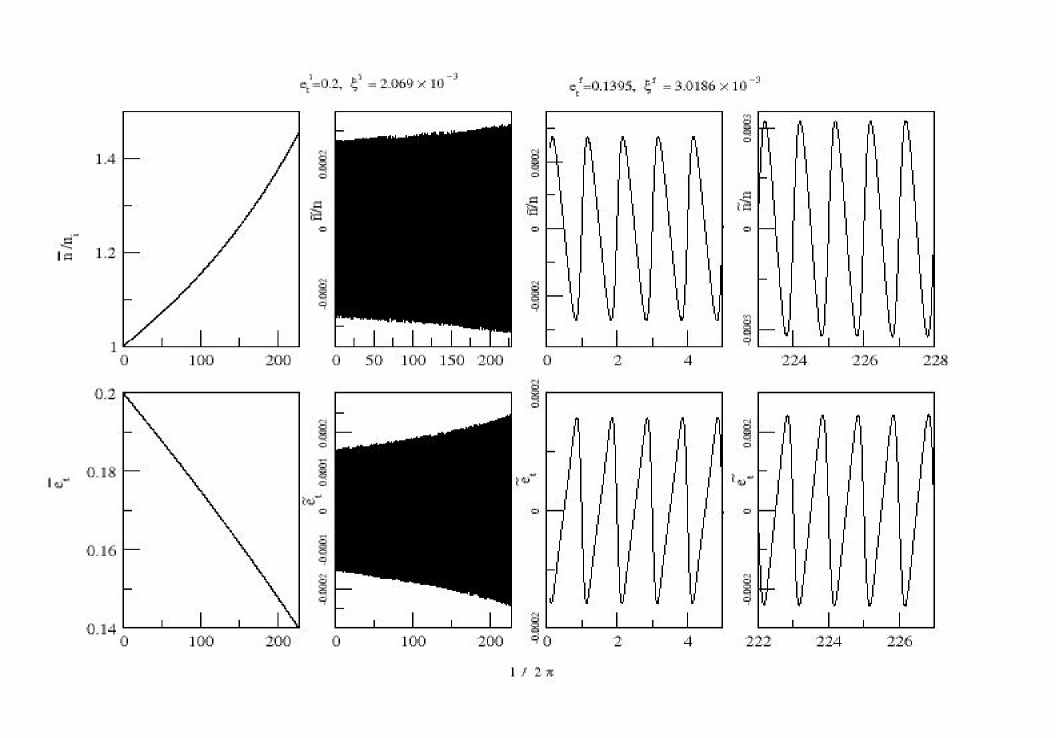
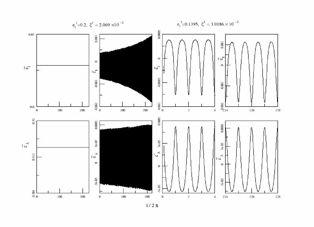
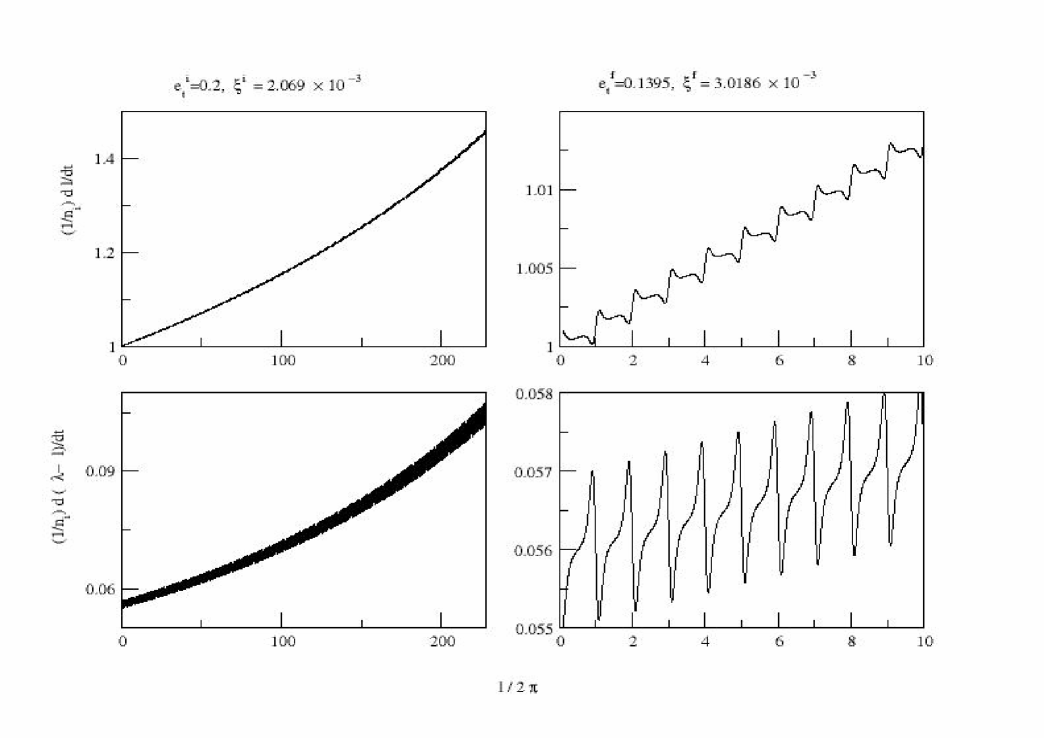
We begin the subsection by illustrating the temporal evolution of $\bar{c}_{\alpha}$ and $\tilde{c}_{\alpha}$. Next, we show the combined effects of these secular and periodic variations on basic angular variables that appear in the expressions for $h_{\times}$ and $h_{+}$. Finally, we exhibit $h_{\times}$ and $h_{+}$ evolving under gravitational radiation reaction and point out various features associated with post-Newtonian accurate orbital motion. In these figures, we terminate the orbital evolution when $j^{2}=48$. This criterion, as explained earlier, is chosen to make sure that the orbit under investigation is a shrinking slowly precessing ellipse. We have also taken advantage of the ‘scaling’ nature of the problem to plot only dimensionless quantities in terms of dimensionless variables. The conversion to familiar quantities like orbital frequency $f$ (in Hertz) is given by $f\equiv\frac{n}{2\,\pi}=\frac{1}{2\,\pi}\,\frac{c^{3}\,\xi}{G\,m}=3.2312\times 10^{4}\,\xi\,\frac{M_{\odot}}{m}$. This implies that for a compact binary with $m=M_{\odot}$ and $\xi=10^{-3}$, the orbital frequency will be $\sim 30$ Hertz.

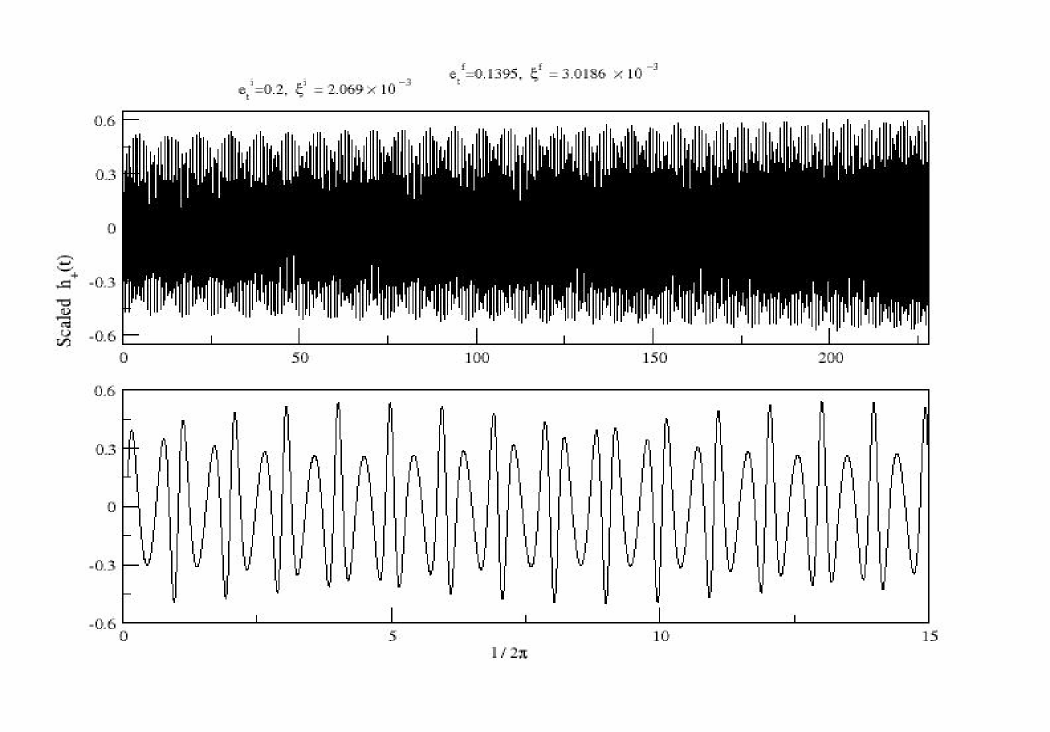
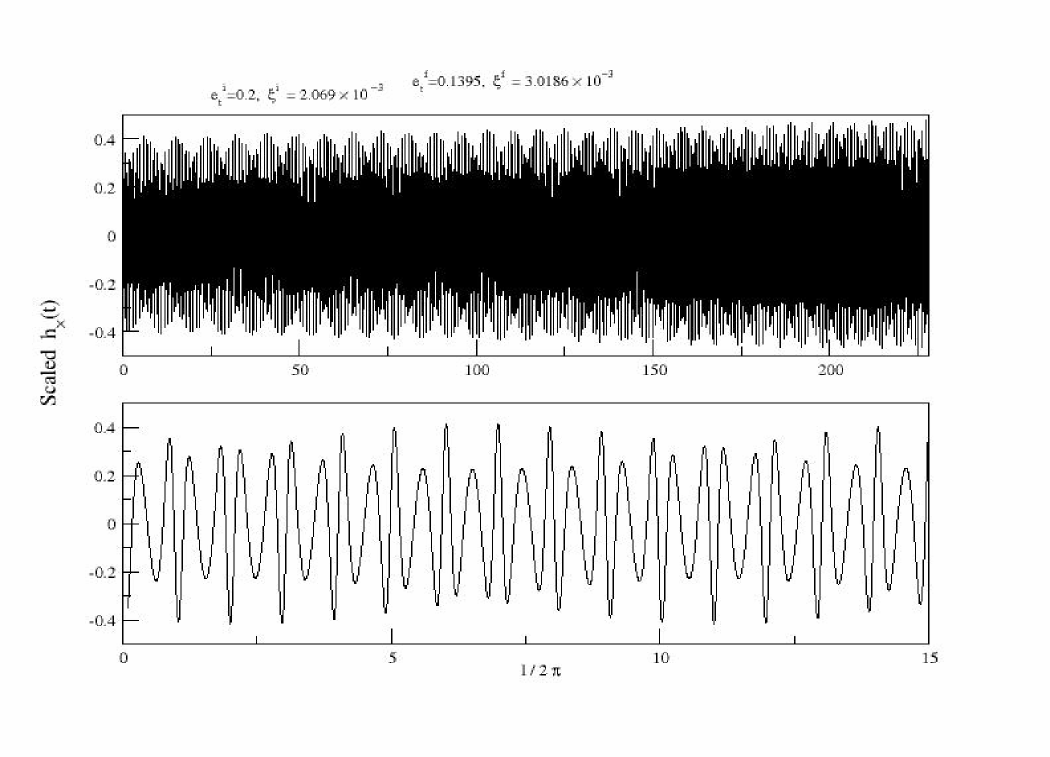
In Figs. (2) and (3), we plot $\bar{n}/n_{i}$ (where $n_{i}$ is the initial value of $n$), $\tilde{n}/n,\bar{e}_{t},\tilde{e}_{t},\bar{c}_{l},\tilde{c}_{l}$, $\bar{c}_{\lambda}$ and $\tilde{c}_{\lambda}$ as functions of $\frac{l}{2\,\pi}$, which gives evolution in terms of elapsed orbital cycles. We clearly see an adiabatic increase (decrease) of $\bar{n}$ $(\bar{e}_{t})$ as well as the periodic variations of $\tilde{n}$ and $\tilde{e}_{t}$. As expected, we also observe no secular evolution for $\bar{c}_{l}$ and $\bar{c}_{\lambda}$, but clearly see periodic variations in $\tilde{c}_{l}$ and $\tilde{c}_{\lambda}$. In order to illustrate the effect of the secular and periodic variations in the above orbital variables on the basic angles $l$ and $\lambda$, in Fig. (4), we plot scaled $dl/dt$ and $d(\lambda-l)/dt$ as functions of $\frac{l}{2\,\pi}$. The figure shows periodic oscillations superposed on the slow secular drift. Finally, in Figs. (5) and (6), we plot scaled $h_{+}$ and $h_{\times}$ as functions of $\frac{l}{2\,\pi}$. We employ, for these figures, polarization amplitudes, which are Newtonian accurate while the orbital motion is 2.5PN accurate. We clearly see ‘chirping’ due to radiation damping, amplitude modulation due to periastron precession and also orbital period variations.

Using the scaling argument mentioned earlier, we note that Figs. (2)-(6) may be used to illustrate the various aspects of a compact binary inspiral from sources relevant for both LIGO and LISA. For instance, if we choose $m=2.8M_{\odot}$, the variation of $\xi$ from $2.069\times 10^{-3}$ to $3.0186\times 10^{-3}$ in around $227$ orbital cycles corresponds to orbital frequency variation from $150$ Hz to $\sim 217$ Hz in $\sim 8.15$ seconds. Similarly, the choice $m=10^{5}M_{\odot}$ corresponds to a binary inspiral involving two supermassive black holes, where orbital frequency increases from $\sim 4.2\times 10^{-3}$ Hz to $\sim 6.2\times 10^{-3}$ Hz in $\sim 2.7$ days.

Finally, we note that Figs. (2)-(6), were drawn mainly to exhibit more clearly the existence of periodic variations in orbital elements (analytically investigated for the first time in the present paper) due to the radiation reaction. Evidently, as these variations scale as $\xi^{5/3}$, see Eqs.(62), they become quite small if the binary is not near the plunge boundary. Our work is important, even when the binary is not near the LSO, as it shows, in a technically clear manner, how to describe the exact phasing as the sum of the usually considered ‘adiabatic’ phasing (involving only secular variations) and a normally neglected ‘post-adiabatic’ phasing (involving only the relatively smaller ‘periodic’ variations). More about this in the conclusions below.

VI PN accurate adiabatic evolution for $\bar{n}$ and $\bar{e}_{t}$

One of the useful results of the present work are Eqs. (56) and (57). Indeed, these equations provide a clear justification for the usually considered ‘adiabatic’ approximation (in cases, where one is sufficiently away from the plunge boundary so that one can safely neglect the additional periodic contributions and treat orbits to be quasi-Keplerian). More precisely, we have, earlier, proved that Eqs. (56) would be valid, even if we are considering radiation reaction to the accuracy ${\cal O}(c^{-5})+{\cal O}(c^{-7})+{\cal O}(c^{-8})+{\cal O}(c^{-9})$. Concerning Eqs. (57), following its derivation again, we see that (if we were to define $c_{a}$ to sufficient accuracy, by considering the conserved quantities of the ‘conservative part’ of the dynamics) it is valid up to terms which are quadratic in the radiation reaction, i.e up to ${\cal O}(c^{-10})$. Therefore, to those very high accuracies, our work shows that the secular part of the phasing (in the sense of the decomposition, as in Eq. (40) ) is essentially given by the simple averaged result, given by Eqs. (56) and (57). Then, as usual, we expect that the averaged losses of the mechanical energy and angular momentum of the system, appearing in Eqs. (57), are equal to the corresponding far zone (FZ) fluxes of energy and angular momentum in the form of radiated gravitational waves.

To complete this work, let us briefly show how to obtain, in ADM coordinates, the 2PN accurate secular changes in $\bar{n}$ and $\bar{e}_{t}$, equivalent to corresponding 2PN accurate FZ fluxes of energy and angular momentum. The differential equations for $\bar{n}$ and $\bar{e}_{t}$ are computed, following the PN accurate calculations presented in GS89 . These computations require PN corrections to orbital averaged expressions for the far-zone energy and angular momentum fluxes and PN accurate expressions for $n$ and $e_{t}$, all of these expressed in terms of orbital energy and angular momentum. The PN accurate expressions for $\frac{d\bar{n}}{dt}$ and $\frac{d\bar{e}_{t}}{dt}$ are obtained by differentiating PN accurate expressions for $n$ and $e_{t}$ w.r.t. time and then heuristically equating the time derivatives of orbital energy and angular momentum to orbital averaged expressions for the far-zone energy and angular momentum fluxes. For the ease of implementation, we split 2PN accurate computations of $\frac{d\bar{n}}{dt}$ and $\frac{d\bar{e}_{t}}{dt}$ into two parts. The first part deals with the purely ‘instantaneous’ 2PN corrections and the second part considers the so called ‘tail’ contributions, appearing at the 1.5PN (reactive) order Def_Inst . The computations to get ‘instantaneous’ contributions begin with 2PN corrections to far-zone fluxes, in harmonic gauge, in terms of $r,\dot{r}$ and $v^{2}$ available in GI97 . Using 2PN accurate relations connecting the dynamical variables in harmonic and ADM coordinates, given by Eqs. (71) in Appendix A, we obtain expressions for the far-zone fluxes in ADM coordinates. These far-zone fluxes are orbital averaged, using 2PN accurate generalized quasi-Keplerian parametrization for elliptical orbits, following lower PN computations done in GS89 . We then compute time derivative of PN accurate expressions for $n$ and $e_{t}$ and equate resulting time derivatives of orbital energy and angular momentum to orbital averaged expressions for the far-zone energy and angular momentum fluxes respectively, to get PN accurate $\frac{d\bar{n}}{dt}$ and $\frac{d\bar{e}_{t}}{dt}$ in terms of $E,j,m$ and $\eta$. Finally, we use Eqs. (47) to obtain the differential equations for $\bar{n}$ and $\bar{e}_{t}$ in terms of $n,e_{t},m$ and $\eta$. The tail contributions to $\frac{d\bar{n}}{dt}$ and $\frac{d\bar{e}_{t}}{dt}$ are already available, in slightly different forms, in GS89 and we only rewrite these expressions in our $n$ and $e_{t}$ variables. Adding these ‘instantaneous’ and ‘tail’ contributions gives us the following 2PN accurate evolution equations for $\bar{n}$ and $\bar{e}_{t}$.

$$\frac{d\bar{n}}{dt} = \frac{(G\,m\,n)^{11/3}\,\eta}{G^{2}\,m^{2}\,c^{5}}\biggl{\{}{\dot{\bar{n}}}^{{\rm N}}+{\dot{\bar{n}}}^{1\,{\rm PN}}+{\dot{\bar{n}}}^{1.5\,{\rm PN}}+{\dot{\bar{n}}}^{2\,{\rm PN}}\biggr{\}}\,,$$ (66a)

$$\frac{d\bar{e}_{t}}{dt} = -\frac{(G\,m\,n)^{8/3}\,\eta\,e_{t}}{G\,m\,c^{5}}\biggl{\{}{\dot{\bar{e_{t}}}}^{{{\rm N}}}+{\dot{\bar{e_{t}}}}^{1\,{\rm PN}}+{\dot{\bar{e_{t}}}}^{1.5\,{\rm PN}}+{\dot{\bar{e_{t}}}}^{2\,{\rm PN}}\,,\biggr{\}}$$ (66b)

where ${\dot{\bar{n}}}^{{\rm N}},{\dot{\bar{n}}}^{1\,{\rm PN}}{\dot{\bar{n}}}^{2\,{\rm PN}},{\dot{\bar{e_{t}}}}^{{\rm N}},{\dot{\bar{e_{t}}}}^{1\,{\rm PN}}$ and ${\dot{\bar{e_{t}}}}^{2\,{\rm PN}}$ denote ‘instantaneous’ contributions to 2PN order, while ${\dot{\bar{n}}}^{1.5\,{\rm PN}}$ and ${\dot{\bar{e_{t}}}}^{1.5\,{\rm PN}}$ stand for the ‘tail’ contributions. Using 2PN accurate orbital representation and far-zone energy and angular momentum fluxes, we have computed 2PN accurate ‘instantaneous’ contributions to $\frac{d\bar{n}}{dt}$ and $\frac{d\bar{e}_{t}}{dt}$, whose explicit forms are given by

$${\dot{\bar{n}}}^{{\rm N}} = \biggl{\{}\frac{1}{5\,(1-e_{t}^{2})^{7/2}}\biggl{[}96\,+292\,e_{t}^{2}+37\,e_{t}^{4}\biggl{]}\biggl{\}}\,,$$ (67a)

$${\dot{\bar{n}}}^{1\,{\rm PN}} = \frac{\xi^{2/3}}{280\,(1-e_{t}^{2})^{9/2}}\biggl{\{}20368-14784\,\eta+\left(219880-159600\,\eta\right)\,e_{t}^{2}$$ (67b)

$$+\left(197022-141708\,\eta\right)\,e_{t}^{4}+\left(11717-8288\,\eta\right)\,e_{t}^{6}\biggr{\}}\,,$$

$${\dot{\bar{n}}}^{2\,{\rm PN}} = \frac{\xi^{4/3}}{30240\,(1-e_{t}^{2})^{11/2}}\biggl{\{}\biggl{(}12592864-13677408\,\eta+1903104\,{\eta}^{2}\biggr{)}$$ (67c)

$$+\biggl{(}131150624-217822752\,\eta+61282032\,{\eta}^{2}\biggr{)}\,e_{t}^{2}$$

$$+\biggl{(}282065448-453224808\,\eta+166506060\,\eta^{2}\biggr{)}\,e_{t}^{4}$$

$$+\biggl{(}112430610-144942210\,\eta+64828848\,{\eta}^{2}\biggr{)}\,e_{t}^{6}$$

$$+\biggl{(}3523113-3259980\,\eta+1964256\,{\eta}^{2}\biggr{)}\,e_{t}^{8}$$

$$-3024\,\biggl{(}96+4268\,e_{t}^{2}+4386\,e_{t}^{4}+175\,e_{t}^{6}\biggr{)}\left(2\,\eta-5\right){\sqrt{1-e_{t}^{2}}}\biggr{\}}\,,$$

$${\dot{\bar{e_{t}}}}^{{\rm N}} = \biggl{\{}\frac{1}{15\,(1-e_{t}^{2})^{5/2}}\biggl{[}304+121\,e_{t}^{2}\biggr{]}\biggr{\}}\,,$$ (67d)

$${\dot{\bar{e_{t}}}}^{1\,{\rm PN}} = \frac{\xi^{2/3}}{2520\,(1-e_{t}^{2})^{7/2}}\biggl{\{}340968-228704\,\eta+\left(880632-651252\,\eta\right)\,e_{t}^{2}$$ (67e)

$$+\left(125361-93184\,\eta\right)\,e_{t}^{4}\biggr{\}}\,,$$

$${\dot{\bar{e_{t}}}}^{2\,{\rm PN}} = \frac{\xi^{4/3}}{30240\,(1-e_{t}^{2})^{9/2}}\biggl{\{}20621680-28665360\,\eta+4548096\,{\eta}^{2}$$ (67f)

$$+\biggl{(}86398044\,-148804812\,\eta+48711348\,{\eta}^{2}\biggr{)}\,e_{t}^{2}$$

$$+\biggl{(}69781286\,-95827362\,\eta+42810096\,{\eta}^{2}\biggr{)}\,e_{t}^{4}$$

$$+\biggl{(}3786543\,-4344852\,\eta+2758560\,{\eta}^{2}\biggr{)}\,e_{t}^{6}$$

$$-1008\,\biggl{(}2672+6963\,e_{t}^{2}+565\,e_{t}^{4}\biggr{)}\left(2\,\eta-5\right)\sqrt{1-e_{t}^{2}}\biggr{\}}\,,$$

where, as in earlier instances, $n$ and $e_{t}$ on the right hand side of these equations stand for $\bar{n}$ and $\bar{e}_{t}$.

The ‘tail’ contributions to $\frac{d\bar{n}}{dt}$ and $\frac{d\bar{e}_{t}}{dt}$, which appear at 1.5PN order, are derivable using Keplerian orbital parameterization and ‘tail’ corrections to orbital averaged expressions for the far-zone energy and angular momentum fluxes available in BS93 ; RS97 . For the ease of presentation, we display below ‘tail’ contributions to $\frac{d\bar{n}}{dt}$ and $\frac{d{\bar{e}_{t}}^{2}}{dt}$, rather than $\frac{d\bar{n}}{dt}$ and $\frac{d\bar{e}_{t}}{dt}$

$$\biggl{(}\frac{d\bar{n}}{dt}\biggr{)}{\bigg{|}}_{\rm Tail} = \frac{384}{5}\,\frac{(G\,m\,n)^{(14/3)}\,\pi\,\eta}{G^{2}\,m^{2}\,c^{8}}\,\kappa_{\rm E}\,,$$ (68a)

$$\biggl{(}\frac{d{\bar{e}_{t}}^{2}}{dt}\biggr{)}{\bigg{|}}_{\rm Tail} = -\frac{256}{5}\,\frac{(G\,m\,n)^{(11/3)}\,\pi\,\eta}{G\,m\,c^{8}}\biggl{\{}(1-e_{t}^{2})\,\kappa_{\rm E}-\sqrt{1-e_{t}^{2}}\,\kappa_{\rm J}\biggr{\}}\,,$$ (68b)

where both $\kappa_{\rm E}$ and $\kappa_{\rm J}$ are expressible in terms of infinite sums involving quadratic products of Bessel functions $J_{p}(p\,e_{t})$ and its derivative $J^{\prime}_{p}(p\,e_{t})$. For completeness, the explicit expressions for $\kappa_{\rm E}$ and $\kappa_{\rm J}$, given in BS93 ; RS97 , are listed below

$$\kappa_{\rm E} = \sum_{p=1}^{+\infty}\frac{p^{3}}{4}\biggl{\{}(J_{p}(p\,e_{t}))^{2}\biggl{[}\frac{1}{e_{t}^{4}}-\frac{1}{e_{t}^{2}}+\frac{1}{3}+p^{2}\biggl{(}\frac{1}{e_{t}^{4}}-\frac{3}{e_{t}^{2}}+3-e_{t}^{2}\biggr{)}\biggr{]}$$ (69a)

$$+p\,\biggl{[}-\frac{4}{e_{t}^{3}}+\frac{7}{e_{t}}-3\,e_{t}\biggr{]}J_{p}(p\,e_{t})\,J^{\prime}_{p}(p\,e_{t})+(J^{\prime}_{p}(p\,e_{t}))^{2}\biggl{[}\frac{1}{e_{t}^{2}}-1$$

$$+p^{2}\left(\frac{1}{e_{t}^{2}}-2+e_{t}^{2}\right)\biggr{]}\biggr{\}}\,,$$

$$\kappa_{\rm J} = \sum_{p=1}^{+\infty}\frac{p^{2}}{2}\sqrt{1-e_{t}^{2}}\biggl{\{}p\,\biggl{[}\frac{3}{e_{t}^{2}}-\frac{2}{e_{t}^{4}}-1\biggr{]}\,(J_{p}(p\,e_{t}))^{2}+\biggl{[}\frac{2}{e_{t}^{3}}-\frac{1}{e_{t}}$$ (69b)

$$+2\,p^{2}\biggl{(}\frac{1}{e_{t}^{3}}-\frac{2}{e_{t}}+e_{t}\biggr{)}\biggr{]}J_{p}(p\,e_{t})\,J^{\prime}_{p}(p\,e_{t})+2\,p\biggl{(}1-\frac{1}{e_{t}^{2}}\biggr{)}\,(J^{\prime}_{p}(p\,e_{t}))^{2}\biggr{\}}\,.$$

We have checked that to 1PN order the above equations are consistent with expressions for $\frac{d\bar{a}_{r}}{dt}$ and $\frac{d\bar{e}_{r}}{dt}$, computed in GS89 . At 2PN order, the above expressions are also consistent with corrected formulae for $\frac{d\bar{a}_{r}}{dt}$ and $\frac{d\bar{e}_{r}}{dt}$, available in GI97 ; GI03er .

VII Conclusion

Let us summarize what we have proposed in this paper and point out possible extensions. We have provided a method for analytically constructing high-accuracy templates for the gravitational wave signals emitted by compact binaries when they move in inspiralling slowly precessing eccentric orbits. In contrast to the simpler problem of modeling the gravitational wave signals emitted by inspiralling circular orbits, which contain only two different time scales (orbital period and radiation reaction time scale), the case of inspiralling eccentric orbits involves three different time scales: orbital period, periastron precession and radiation-reaction time scales. An improved ‘method of variation of constants’ is used to combine these three time scales, without making the usual approximation of treating adiabatically the radiative time scale. By going to a suitable center-of-mass frame, the transverse traceless (TT) radiation field and hence the GW polarizations are expressed as PN expansions of the form given in Eq. (4) in harmonic coordinates involving only the relative position and velocity. The polarisations can be rewritten in terms of the ADM positions and velocities by using the contact transformations available to move from the harmonic coordinates to the ADM coordinates. In the ADM coordinates, the unperturbed 2PN (3PN) motion may be explicitly solved by a generalized quasi-Keplerian representation involving two angles $l$ and $\lambda$ and four constants of the 2PN (3PN) motion $c_{\alpha}=c_{1},c_{2},c_{l}$ and $c_{\lambda}$. By a Lagrange method of variation of constants, this unperturbed solution is used to prescribe a general solution to the perturbed (by radiation-reaction) system of the form given by Eqs. (32) and (33), in terms of the varying $c_{\alpha}$’s. Among the four $c_{\alpha}$’s, two ($c_{l}$ and $c_{\lambda}$) are found to be constants, while the other two $c_{\alpha}$’s satisfy two coupled first order differential equations. A two scale decomposition of the $c_{\alpha}$’s is made to model the combination of the slow (radiation reaction, secular) drift and the fast (orbital time scale, periodic) oscillations. This allows us to decompose the TT gravitational wave amplitudes or polarizations into a part associated with the secular variations and another part associated with the fast oscillations. If one expands in the fast oscillations, the oscillatory contributions to the phasing would be equivalent to new additional ${\cal{O}}(v^{5}/c^{5})$ contributions (which stay always small ) to be added to the usually considered 2.5PN amplitude $h_{ij}^{5}$ in the adiabatic approximation. Therefore, as long as an amplitude correction ${\cal{O}}(v^{5}/c^{5})$ is not needed our results show that it is enough to use only secularly varying $\bar{n}$ and $\bar{e}_{t}$. Note that our description of secular effects automatically include an effect of a secular acceleration of the periastron precession, analogous to the usual secular acceleration of the orbital motion. Namely, the secular part of the angle $\lambda-l$ measuring the periastron longitude varies as

$$\bar{\lambda}-\bar{l}=\int\bar{k}\bar{n}dt$$ (70)

where $\bar{k}(t)=\delta\Phi/2\pi$ is the secularly varying periastron precession per orbital period.

Schematically, thus our work may be summarized as follows:

In this paper, the orbit of the binary was treated to be an inspiralling, slowly precessing ellipse, which prevented us from approaching the LSO. However, as mentioned earlier, using the EOB approach, we intend to explore the orbital dynamics and hence the evolution of gravitational wave polarizations near the LSO in the near future. There are also quite a few generalizations which can be tackled using the formalism presented here and we list a few of them here. In this paper, the conservative dynamics was restricted to the 2PN order and therefore, a natural extension will be to incorporate the 3PN conservative dynamics. We also restricted our approach to compact binaries consisting of non-spinning point masses. It is possible to extend the generalized quasi-Keplerian parametrization and hence our method to spinning compact binaries. To do that, first, one needs to extend the quasi-Keplerian representation to include the effects due to spin-orbit and spin-spin interactions, which requires generalizing a restricted analysis done in W95 and this is under investigation KG04 . Finally, starting from the gravitational wave polarizations from inspiralling eccentric binaries in the time-domain, it should be possible to perform a spectral analysis and see how their power spectrum depends on various orbital elements like $n$, $e_{t}$ and $i$.

Appendix A The construction of PN corrections to $h_{\times}$ and $h_{+}$

In this appendix, we sketch the procedure to compute PN corrections to $h_{+}$ and $h_{\times}$ in ADM coordinates, in terms of the dynamical variables $r,\dot{r},\phi$ and $\dot{\phi}$. It is clear from Eqs. (1), (3) and (6) that PN corrections $h_{+}$ and $h_{\times}$ require PN corrections to $h_{ij}^{\rm TT}$. The ‘instantaneous’ 2PN accurate contributions to $h_{ij}^{\rm TT}$ in harmonic coordinates in terms of the components of ${\bf n}$ and ${\bf v}$, $r,\dot{r}$ and $v^{2}$ were computed in GI97 . To obtain similar expressions in ADM coordinates, we employ the 2PN accurate contact transformations linking the harmonic and ADM coordinates, given in DS85 , which prescribe the way to relate the dynamical variables in these coordinates. We list below the transformation equations relating ${\bf x}$ and ${\bf v}$ in the harmonic coordinates to the corresponding ones in ADM GI03er :

$${\bf x}_{\rm H} = {\bf x}_{\rm A}+{Gm\over 8\,c^{4}\,r}\left\{\left[\left(5v^{2}-\dot{r}^{2}\right)\eta+2\,\left(1+12\eta\right){Gm\over r}\right]{\bf x}\right.$$ (71a)

$$\left.-18\,\eta\,r\dot{r}\,{\bf v}\right\}\,,$$

$${\bf v}_{\rm H} = {\bf v}_{\rm A}-{Gm\dot{r}\over 8\,c^{4}\,r^{2}}\biggl{\{}\biggl{[}7v^{2}+38{Gm\over r}-3\dot{r}^{2}\biggr{]}\eta+4\,{Gm\over r}\,\biggr{\}}{\bf x}$$ (71b)

$$-{Gm\over 8\,c^{4}r}\biggl{\{}\biggl{[}13\,v^{2}-17\dot{r}^{2}-42{Gm\over r}\biggr{]}\eta-2\,{Gm\over r}\biggr{\}}{\bf v}\,.$$

The subscripts ‘${\rm H}$’ and ‘${\rm A}$’ denote quantities in the harmonic and in the ADM coordinates respectively. Note that in all the above equations the differences between the two gauges are at the 2PN order and hence no suffix is used for the 2PN terms. We do not list the transformation relations for $r,\dot{r}$ and $v^{2}$ as they easily follow from Eqs. (71), as $r=|{\bf x}|,r\,\dot{r}={\bf x}\cdot{\bf v}$ and $v^{2}={\bf v}\cdot{\bf v}=\dot{r}^{2}+r^{2}\,\dot{\phi}^{2}$.

Using Eqs.(71), the 2PN corrections to $h_{ij}^{TT}$ in ADM coordinates can easily be obtained from Eqs. (5.3) and (5.4) of GI97 . For economy of presentation, we write $(h_{ij}^{TT})_{\rm A}$ in the following manner, $(h_{ij}^{TT})_{\rm A}=(h_{ij}^{TT})_{\rm O}+$ ‘$Corrections$’, where $(h_{ij}^{TT})_{\rm A}$ represent the metric perturbations in the ADM coordinates. $(h_{ij}^{TT})_{\rm O}$ is a short hand notation for expressions on the R.H.S of Eqs. (5.3) and (5.4) of GI97 , where ${\bf N},{\bf n},{\bf v},v^{2},\dot{r},r$ are the ADM variables ${\bf N}_{\rm A},{\bf n}_{\rm A},{\bf v}_{\rm A},v_{\rm A}^{2},{\dot{r}}_{\rm A},r_{\rm A}$ respectively. The ‘$Corrections$’ represent the differences at the 2PN order, that arise due to the change of the coordinate system, given by Eqs. (71). As the two coordinates are different only at the 2PN order, the ‘$Corrections$’ come only from the leading Newtonian terms in Eqs. (5.3) and (5.4) of GI97 .

$$(h^{TT}_{ij})_{\rm A} = (h^{TT}_{ij})_{\rm O}+{G\over c^{4}\,R}\,{G\,m\over 2\,c^{4}\,r_{\rm A}}\biggl{\{}\biggl{[}(5\,v_{\rm A}^{2}-55\,{\dot{r}}_{\rm A}^{2})\,\eta+2\left(1+12\,\eta\right)\,{G\,m\over r_{\rm A}}\biggr{]}\,{G\,m\over r_{\rm A}}\,(n_{ij})_{\rm A}^{TT}$$ (72)

$$-2\,\biggl{[}(7\,v_{\rm A}^{2}-3\,{\dot{r}}_{\rm A}^{2})\,\eta+4\left(1+5\,\eta\right)\,{G\,m\over r_{\rm A}}\biggr{]}{\dot{r}}_{\rm A}\,(n_{(i}v_{j)})_{\rm A}^{TT}$$

$$-\biggl{[}(26\,v_{\rm A}^{2}-34\,{\dot{r}}_{\rm A}^{2})\,\eta-\left(4+84\,\eta\right)\,{G\,m\over r_{\rm A}}\biggr{]}\,(v_{ij})_{\rm A}^{TT}\biggr{\}}\,.$$

We now have all the inputs required to compute the 2PN corrections to $h_{+}$ and $h_{\times}$ in ADM coordinates, in terms of $r,\phi,\dot{r}$ and $\dot{\phi}$. We write, schematically, the expression for $(h^{TT}_{ij})_{\rm A}$ as

$$(h^{TT}_{ij})_{\rm A}=\alpha_{vv}\,v_{ij}+\alpha_{nn}\,n_{ij}+\alpha_{nv}\,n_{(i}v_{j)}\,.$$ (73)

We apply exactly the same procedure which gave us the Newtonian expressions to $h_{+}$ and $h_{\times}$ from Newtonian contributions to $h^{TT}_{ij}$. Since the explicit expressions for the final 2PN accurate ‘instantaneous’ GW polarization states are too lengthy to be listed here, we write schematically

$$h_{+} = \biggl{\{}\alpha_{vv}\biggl{[}(\cdots)+(\cdots)\cos 2\phi+(\cdots)\sin 2\phi\biggr{]}+\alpha_{nn}\biggl{[}(\cdots)+(\cdots)\cos 2\phi\biggr{]}$$ (74a)

$$+\alpha_{nv}\biggl{[}(\cdots)+(\cdots)\cos 2\phi+(\cdots)\sin 2\phi\biggr{]}\biggl{\}}\,,$$

$$h_{\times} = \biggl{\{}\alpha_{vv}\bigl{[}(\cdots)\cos 2\phi+(\cdots)\sin 2\phi\bigr{]}+\alpha_{nn}\biggl{[}(\cdots)\sin 2\phi\biggr{]}$$ (74b)

$$+\alpha_{nv}\biggl{[}(\cdots)\cos 2\phi+(\cdots)\sin 2\phi\biggr{]}\biggl{\}}.$$

In the above and what follows $\bigl{(}\cdots\bigr{)}$ denotes various coefficients expressed in terms of $r,\dot{r},\dot{\phi},m_{1},m_{2}$ and $i$. The structure of the PN expansion of the coefficients $\alpha_{ij}$ above is the following:

$$\alpha_{vv} \sim 1+\frac{1}{c}\biggl{[}\bigl{(}\cdots\bigr{)}\cos\phi+\bigl{(}\cdots\bigr{)}\sin\phi\biggr{]}+\frac{1}{c^{2}}\biggl{[}\bigl{(}\cdots\bigr{)}+\bigl{(}\cdots\bigr{)}\cos 2\phi+\bigl{(}\cdots\bigr{)}\sin 2\phi\biggr{]}+$$ (75)

$$\frac{1}{c^{3}}\biggl{[}\bigl{(}\cdots\bigr{)}\cos 3\phi+\bigl{(}\cdots\bigr{)}\sin 3\phi\biggr{]}+\frac{1}{c^{4}}\biggl{[}\bigl{(}\cdots\bigr{)}+\bigl{(}\cdots\bigr{)}\cos 4\phi+\bigl{(}\cdots\bigr{)}\sin 4\phi\biggr{]}.$$

$\alpha_{nn}$ and $\alpha_{nv}$ have similar expansions with the exception that for $\alpha_{nv}$ the leading order term is at $1\over c$ order. We note that, similar to Eq. (6), the above sketched expressions for $h_{+}$ and $h_{\times}$ are in a form suitable to apply our phasing formalism.

Figure 1: The 2PN accurate effective radial potential $W_{j}(u)$ as a function of the dimensionless radial variable $\frac{1}{u}=\frac{c^{2}\,R}{G\,m}$, for various values of the dimensionless angular momentum $j$. The point, marked c, denotes a stable circular orbit, while the line, noted e, stands for a precessing elliptical orbit. The line with label p denotes an elliptical orbit which is about to plunge. Note that the left end of the line p is tangent to the effective potential, and corresponds to an unstable circular orbit. The plots are for $\eta=0.25$.

Figure 2: The plots for $\bar{n}/n_{i},\tilde{n}/n,\bar{e}_{t}$ and $\tilde{e}_{t}$ versus $\frac{l}{2\,\pi}$, which gives the number of orbital revolutions. These variations are governed by the reactive 2.5PN equations of motion. Periodic nature of the variations in $\tilde{n}$ and $\tilde{e}_{t}$ are clearly visible. $e_{t}^{i}$ and $e_{t}^{f}$ denote initial and final values for the time eccentricity $e_{t}$, while $\xi^{i}$ and $\xi^{f}$ stand for similar values of the adimensional mean motion $\frac{G\,m\,n}{c^{3}}$. The plots are for $\eta=0.25$ and the evolution is terminated when $j^{2}=48$.

Figure 3: The plots $\bar{c}_{l},\tilde{c}_{l},\bar{c}_{\lambda}$ and $\tilde{c}_{\lambda}$ against orbital cycles, given by $\frac{l}{2\,\pi}$. Similar to Fig. 2, these variations are governed by the reactive 2.5PN equations of motion. Periodic nature of the variations in $\tilde{c}_{l}$ and $\tilde{c}_{\lambda}$ as well as the constancy of $\bar{c}_{l}$ and $\bar{c}_{\lambda}$ are clearly visible. The symbols have the same meaning as in Fig 2.

Figure 4: The plots showing scaled time derivative of $l$ and $\lambda-l$ as function of orbital cycles, given by $\frac{l}{2\,\pi}$. The right panels show clearly both the secular drift and the periodic oscillations of the plotted quantities. Similar to earlier figures, these variations are governed by the reactive 2.5PN equations of motion. The initial and final values of the relevant orbital elements are marked on the plots. The plots are for $\eta=0.25$ and $n_{i}$ is the initial value of the mean motion $n$.

Figure 5: The scaled $h_{+}$ ( Newtonian in amplitude and 2.5PN in orbital motion) plotted against orbital cycles, given by $\frac{l}{2\,\pi}$. The ‘chirping’, amplitude modulation due to periastron precession are clearly visible in the upper panel. In the bottom panel, we zoom into the initial stages of orbital evolution to show the effect of the periodic orbital motion and the periastron advance on the scaled $h_{+}(t)$. The initial and final values of the relevant orbital elements are marked on the plots. The plots are for $\eta=0.25$ and the orbital inclination is $i=\frac{\pi}{3}$.

Figure 6: The plots for the scaled $h_{\times}$ (Newtonian in amplitude and 2.5PN in orbital motion) as function of $\frac{l}{2\,\pi}$, where $l$ is the mean anomaly . The slow ‘chirping’, amplitude modulation due to periastron precession are clearly visible in the upper panel. In the bottom panel, we zoom into the initial stages of orbital evolution to show the effect of the periodic orbital motion and the periastron advance on the scaled $h_{\times}(t)$. The initial and final values of the relevant orbital elements are marked on the plots. The plots are for a binary consisting of equal masses, such that $\eta=0.25$ and the orbital inclination is $i=\frac{\pi}{3}$. The orbital evolution, as in earlier cases, is terminated when $j^{2}=48$.

References

- (1) Following URLs provide a wealth of information about the terrestrial gravitational wave interferometers. http://www.ligo.caltech.edu, http://www.virgo.infn.it, http://www.geo600.uni-hannover.de, and http://tamago.mtk.nao.ac.jp.
- (2) L. P. Grishchuk, V. M. Lipunov, K. A. Postnov, M. E. Prokhorov, and B. S. Sathyaprakash, Phys. Usp. 44, 1 (2001); Usp. Fiz. Nauk 171, 3 (2001), (astro-ph/0008481).
- (3) There are a large number of research articles which investigate issues related to the construction of accurate and efficient ‘ready to use‘ search templates for compact binaries of arbitrary mass ratio, moving mainly in quasi-circular orbits. See e.g. T. Damour, B. R. Iyer and B. S. Sathyaprakash, Phys. Rev. D 63 , 044023 (2001); ibid 66, 027502 (2002) and references therein. Issues related to binary black holes are exhaustively dealt in A. Buonanno, Y. Chen and M. Vallisneri, Phys. Rev. D 67, 024016 (2003) and T. Damour, B. R. Iyer, P. Jaranowski and B. S. Sathyaprakash Phys. Rev. D 67, 064028, (2003).
- (4) P. C. Peters, Phys. Rev. 136, B1224 (1964).
- (5) M. C. Miller and D. P. Hamilton, Astrophys. J. 576, 894, (2002).
- (6) Y. Kozai, Astro. J. 67, 591, (1962).
- (7) L. Wen, On the Eccentricity Distribution of Coalescing Black Hole Binaries Driven by the Kozai Mechanism in Globular Clusters, (astro-ph/0211492)
- (8) http://lisa.jpl.nasa.gov
- (9) M. J. Benacquista, Class. Quantum Grav. 19, 1297 (2002)
- (10) K. S. Thorne and V. B. Braginsky, Astrophys. J. 204, L1, (1976).
- (11) S. Sigurdsson, Workshop summary for Massive black holes coalescence focus session, Penn State, 2002, (gr-qc/0303027).
- (12) O. Blaes, M. H. Lee and A. Socrates, Astrophys. J. 578, 775, (2002).
- (13) H. Sudou, S. Iguchi, Y. Murata and Y. Taniguchi, Science, 300, 1263, (2003).
- (14) P. C. Mathews and J. Mathews, Phys. Rev. B 136, 435 (1963).
- (15) H. Wahlquist, Gen. Rel. Grav. 19, 1101, (1987).
- (16) C. W. Lincoln and C. M. Will, Phys. Rev. D 42, 1123 (1990).
- (17) R. Wagoner and C. M. Will, Astrophys. J. 210, 764, (1976); erratum 215, 984,(1977); L. Blanchet and G. Schäfer, Mon. Not. R. Astron. Soc. 239, 845 (1989); W. Junker and G. Schäfer, Mon. Not. R. Astron. Soc. 254, 146 (1992); L. Blanchet and G. Schäfer, Class. Quantum Grav. 10, 2699 (1993); R. Rieth and G. Schäfer, Class. Quantum Grav. 14, 2357 (1997);
- (18) C. Moreno-Garrido, J. Buitrago and E. Mediavilla, Mon. Not. R. Astron. Soc. 274, 115 (1995).
- (19) C. Moreno-Garrido, J. Buitrago and E. Mediavilla, Mon. Not. R. Astron. Soc. 266, 16 (1994).
- (20) K. Martel and E. Poisson, Phys.Rev. D60, 124008 (1999).
- (21) V. Pierro, I. M. Pinto, A. D. Spallicci, E. Laserra and F. Recano, Mon. Not. R. Astron. Soc. 325, 358 (2001).
- (22) A. V. Gusev, V. B. Ignatiev, A. G. Kuranov, K. A. Postnov, and M. E. Prokhorov, Astron. Lett. 28, 143, (2002).
- (23) N. Seto, Phys. Rev. Lett. 87, 251101 (2001).
- (24) L. Blanchet, T. Damour, B.R. Iyer, C. M. Will and A. G. Wiseman, Phys. Rev. Lett. 74, 3515 (1995); L. Blanchet, T. Damour, and B. R. Iyer, Phys. Rev. D 51, 5360 (1995).
- (25) L. Blanchet, B.R. Iyer, C. M. Will and A. G. Wiseman, Class. Quantum Grav. 13, 575 (1996).
- (26) T. Damour, B. R. Iyer, P. Jaranowski and B. S. Sathyaprakash, Phys. Rev. D 67, 064028, (2003).
- (27) C. M. Will and A. G. Wiseman, Phys. Rev. D 54, 4813 (1996).
- (28) A. Gopakumar and B. R. Iyer, Phys. Rev. D 56, 7708 (1997).
- (29) T. Damour and G. Schäfer, Nuovo Cimento B 101, 127 (1988).
- (30) G.. Schäfer and N. Wex, Phys. Lett. 174 A, 196, (1993); erratum 177, 461.
- (31) A. Gopakumar and B. R. Iyer, Phys. Rev. D 65, 84011 (2002).
- (32) The 2PN corrections to the rate of decay of orbital elements of the generalized quasi-Keplerian representation, computed in GI97 and the 2PN contributions to gravitational wave polarizations found in GI02 are erroneous. These errors were due to an incorrect implementation of the contact transformations between the harmonic and ADM coordinates. As these coordinates are identical to the 1PN order, errors surfaced at 2PN order terms in the ADM coordinates. The errata, correcting these errors, will be published soon. In Appendix A, we present the correct transformations for and in these coordinates.
- (33) T. Damour, in Gravitational Radiation, N. Deruelle and T. Piran (eds.), North-Holand Company (1983).
- (34) T. Damour and N. Deruelle, Ann. Inst. Henri Poincare Phys. Theor. 43, 107 (1985).
- (35) T. Damour and J. Taylor, Phys. Rev D 45 , 1840 (1992).
- (36) T. Damour, Phys. Rev. Lett. 51, 1019 (1983).
- (37) T. Damour in Proceedings of Journées Relativistes 1983, edited by S. Benenti, M. Ferraris and M. Francaviglia ( Pitagora Editrice, Bologna, 1985), pp 89-110.
- (38) K. G. Arun, L. Blanchet, B. R. Iyer and M. S. S. Qusailah, In Preparation, (2004).
- (39) G. Schäfer, Lettere Al Nuovo Cimento, 36, 105 (1983), ibid, Ann. Phys. (N.Y.) 161, 81 (1985); T. Damour and G. Schäfer, Nuovo Cimento B 101, 127 (1988).
- (40) P. Jaranowski and G. Schäfer, Phys. Rev. D 57, 7274 (1998); ibid, 60, 124003 (1999); T. Damour, P. Jaranowski, and G. Schäfer, Phys. Rev. D 62, 021501(R) (2000) [Erratum: 63, 029903(E) (2001)]; ibid 63, 044021, (2001) [Erratum, 66, 029901(E), (2002)]; T. Damour, P. Jaranowski, and G. Schäfer, Phys. Lett. B 513, 147 (2001).
- (41) L. Blanchet and G. Faye, Phys. Lett. A 271, 58 (2000); Phys. Rev. D 63, 062005 (2000); J. Math. Phys. 41, 7675 (2000); ibid 42, 4391 (2001).
- (42) T. Damour, P. Jaranowski and G. Schäfer, Phys. Rev. D 62, 044024, (2000).
- (43) V. C. de Andrade, L. Blanchet, and G. Faye, Class. Quantum Grav. 18, 753, (2001);
- (44) L. Blanchet and B. R. Iyer, Class. Quantum Grav. 20, 755, (2003).
- (45) T. Damour and G. Schäfer, Gen. Rel. Grav. 17, 879, (1985).
- (46) A. Buonanno and T. Damour, Phys.Rev. D 59, 084006 (1999); ibid Phys.Rev. D 62, 064015 (2000).
- (47) T. Damour, P. Jaranowski and G. Schäfer, Phys.Rev. D 62, 084011 (2000).
- (48) K. Glampedakis and D. Kennefick, Phys.Rev. D 66, 044002 (2002).
- (49) We point out a slight mismatch in the definition of used here and in DS88 ; SW93 . We observe that employed in DS88 ; SW93 , say , gives the orbital (non-relativistic) energy per unit reduced mass, which in terms of reads . In this paper, . Similarly, the dimensionless angular momentum variable is related to , used in DS88 ; SW93 , by .
- (50) R.-M. Memmesheimer, A. Gopakumar, S. Menzel, and G. Schäfer, In Preparation, (2004).
- (51) G. Schäfer, Ann. Phys. (N.Y.) 161, 81 (1985); B. R. Iyer and C. M. Will, Phys. Rev. D 52, 6882 (1995); C. Königsdörffer, G. Faye and G. Schäfer Phys. Rev. D 68, 044004 (2003).
- (52) L. Blanchet and T. Damour, Phys. Rev. D 37, 1410 (1988); ibid 46, 4304 (1992).
- (53) L. Blanchet and G. Schäfer, Class. Quantum Grav. 10, 2699 (1993);
- (54) W.H. Whittaker and G.N. Watson, Modern Analysis, CUP, Cambridge (1927).
- (55) Following BDIWW , we term contributions to the GW amplitude and its associated quantities that depend only on the state of the binary at the retarded instant as its ‘instantaneous’ part, whereas the contributions, which are a priori sensitive to the entire ‘history’ of the binary’s dynamics are termed as the ‘tail’ contributions.
- (56) R. Rieth and G. Schäfer, Class. Quantum Grav. 14, 2357 (1997).
- (57) N. Wex, Class. Quantum Grav. 12, 983 (1995).
- (58) C. Königsdörffer and A. Gopakumar, In Preparation, (2004).