A New Waveform Consistency Test for Gravitational Wave Inspiral Searches

Abstract

Searches for binary inspiral signals in data collected by interferometric gravitational wave detectors utilize matched filtering techniques. Although matched filtering is optimal in the case of stationary Gaussian noise, data from real detectors often contains “glitches” and episodes of excess noise which cause filter outputs to ring strongly. We review the standard $\chi^{2}$ statistic which is used to test whether the filter output has appropriate contributions from several different frequency bands. We then propose a new type of waveform consistency test which is based on the time history of the filter output. We apply one such test to the data from the first LIGO science run and show that it cleanly distinguishes between true inspiral waveforms and large-amplitude false signals which managed to pass the standard $\chi^{2}$ test.

pshawhan@ligo.caltech.edu

• Submitted to Class. Quantum Grav.for GWDAW-8 Proceedings issue

1 Introduction

A binary system of two neutron stars or black holes in a close orbit loses energy and angular momentum through the emission of gravitational radiation, causing the orbital distance to decrease. In the final “inspiral” stage of this evolution, the emitted gravitational waves rise in frequency and amplitude at an accelerating rate, until the orbit becomes unstable and the objects coalesce. The exact form of this “chirp” waveform depends on the masses and spins of the binary components. In the case of a double neutron star system, the inspiral waveform spends many seconds within the sensitive frequency band of the large ground-based interferometric gravitational wave detectors which are now collecting scientific data or are being commissioned (TAMA300, LIGO, GEO 600, and VIRGO), and spin effects are believed to be negligible. Thus, template waveforms for these systems can be calculated accurately and can be used to search for this class of signals by matched filtering [1, 2], which performs a phase-coherent correlation of the data with the template, varying the coalescence time parameter. Binary systems involving low-mass black holes (up to perhaps $\sim$$50~{}M_{\odot}$) also inspiral within the frequency band of ground-based interferometers and can be searched for with matched filtering, although the higher mass implies shorter template durations (down to $\ll$$1$ s) and more severe relativistic and spin effects, requiring searches to be done in an expanded parameter space [4].

Simple matched filtering is the optimal detection strategy if the detector noise is stationary and white. In the case of stationary colored noise, optimal performance is obtained by filtering in the frequency domain with a weight inversely proportional to the power spectral density of the noise, as we will review briefly in section 2. However, real gravitational wave detectors are commonly found to suffer from non-stationarity, either in the form of “glitches” (highly localized in time) or as roughly adiabatic variation of the broadband noise level over short time scales. Either type of non-stationarity can strongly excite a matched filter, leading to false “triggers” when the filter output amplitude exceeds a predetermined threshold. Therefore, it has become standard to test the consistency of the trigger-generating data with the template waveform by calculating a $\chi^{2}$ statistic, defined in section 3. This value is normally small for a real signal but tends to be large for triggers caused by non-stationary noise.

Rejecting triggers with large $\chi^{2}$ eliminates many inspiral triggers caused by non-stationary noise, but some manage to pass this test. This became particularly clear in follow-up examination of inspiral event candidates found by the analysis of the first LIGO science run (called “S1” [6]), as illustrated in section 4. Guided by the characteristics of these event candidates, in this paper we propose a new type of waveform consistency test which is based on the time history of the output of the matched filter in the vicinity of the trigger. As described in section 5, this type of test has the advantage of being simple to implement and has negligible computational cost. In section 6, we apply an empirically chosen test of this type to the LIGO S1 data and show that it eliminates many of the largest-amplitude triggers found by the S1 inspiral search without reducing the efficiency for detecting real signals. Although the choice and tuning of a test of this type depends on the exact nature of the non-stationarity in the detector noise, it is reasonable to expect that waveform consistency tests of this type may lead to significantly cleaner inspiral searches when analyzing data from other science runs and other detectors.

2 Review of matched filtering for inspiral searches

We will focus on matched filtering as implemented for the search for binary neutron star inspirals in LIGO S1 data [7], using similar notation. An inspiral produces a gravitational wave strain in the interferometer, $h(t)$, which depends on the intrinsic physical properties of the binary system, the coalescence time $t_{c}$, and the position and orientation of the system relative to the interferometer. For low-mass systems, the masses of the two components are the only relevant physical parameters. The effect of the position and orientation of the system on the received signal can be represented by just two parameters, an effective distance $D_{\rm eff}$ and a signal phase $\alpha$. Thus, we may represent a template waveform as $h^{I}(t-t_{c};\alpha)$, where the index $I$ represents a point in the space of intrinsic parameters and the template is normalized to correspond to a signal with a certain effective distance. From this point onward we will omit the index $I$, so that the formulae will refer to any individual template from the “bank” of templates which is used to cover a region of intrinsic parameter space.

A further simplification is obtained by transforming the template to the frequency domain using the stationary phase approximation [9], so that the template has the form $e^{i\alpha}\tilde{h}_{c}(f)$ where $\tilde{h}_{c}(f)$ is independent of $\alpha$. Thus, we can simply use $\tilde{h}_{c}(f)$ (i.e., the template with $\alpha=0$) to filter the data and then consider the magnitude of the result, effectively maximizing over the signal phase $\alpha$ analytically. The Wiener optimal filter, which dictates that noisy frequencies should be suppressed, is easily applied in the frequency domain to the Fourier-transformed data from the detector, $\tilde{s}(f)$:

$$z(t)=4\int_{0}^{\infty}\frac{\tilde{h}_{c}(f)\tilde{s}^{\ast}(f)}{S_{n}(f)}\,e^{2\pi ift}\;df$$ (1)

where $S_{n}(f)$ is the power spectral density of the detector noise, estimated from nearby data. The output of the matched filter is

$$\rho(t)=\frac{|z(t)|}{\sigma}$$ (2)

where

$$\sigma^{2}=\frac{\left\langle|z(t)|^{2}\right\rangle}{2}=4\int_{0}^{\infty}\frac{\left|\tilde{h}_{c}(f)\right|^{2}}{S_{n}(f)}\;df$$ (3)

normalizes $\rho$ so that it can be interpreted as an amplitude signal-to-noise ratio (SNR). If the detector noise is stationary (and there is no signal present), then $\rho(t)$ will be a random variable with $\left\langle\rho^{2}\right\rangle=2$.

The filter output $\rho(t)$ is evaluated at a set of discrete times $t$ with a time step shorter than the period of the inspiral waveform at its highest frequency. For example, the LIGO S1 analysis used a time step of $1/4096$ s. A true inspiral signal in the data would lead to a narrow peak in $\rho(t)$ at the coalescence time, reflecting the fact that each time sample in the filter output is the appropriate coherent sum of signal power distributed over time and frequency in the input time series. Accordingly, the inspiral search algorithm essentially consists of looking for local maxima of $\rho(t)$ (separated in time by at least the length of the template) which exceed some fixed threshold $\rho^{\ast}$. Each such maximum is called a “trigger”, characterized by $\rho_{\rm max}$, and is subjected to further evaluation. The threshold $\rho^{\ast}$ is chosen for practical reasons, to yield a manageable number of triggers.

3 The standard $\chi^{2}$ test

The technique of calculating a $\chi^{2}$ to check the consistency of a trigger with the expected waveform was developed several years ago [10] and has been utilized in published inspiral searches [12, 13, 7]. The inspiral template is effectively divided into $p$ sub-templates labeled by $l=\{1,2,...,p\}$, each of which contains a different frequency band of the original template. The data is filtered using each of these templates:

$$z_{l}(t)=4\int_{F_{l-1}}^{F_{l}}\frac{\tilde{h}_{c}(f)\tilde{s}^{\ast}(f)}{S_{n}(f)}\,e^{2\pi ift}\;df$$ (4)

where the frequency boundaries $F_{l}$ are chosen so that each of the sub-templates should, in the absence of noise, contribute equally to the total signal, i.e. $\langle z_{l}(t_{c})\rangle=z(t_{c})/p$. Using these values, the $\chi^{2}$ statistic is calculated as

$$\chi^{2}(t)=\frac{p}{\sigma^{2}}\sum_{l=1}^{p}\left|z_{l}(t)-z(t)/p\right|^{2}$$ (5)

evaluated at the inferred coalescence time of the original trigger. Note that this definition demands that the sub-templates be consistent with the full template in both amplitude and phase. If the signal in the data matches the template exactly, then this $\chi^{2}$ statistic will follow a chi-squared distribution with $2p-2$ degrees of freedom.

Figure 1: Graphical representation of the $\chi^{2}$ statistic in a time-frequency plane. The thick black line shows the frequency of the chirp waveform rising with time. The division of the waveform into $p$ frequency bands ($p=8$ in this case, with boundaries indicated by the dotted horizontal lines) essentially creates $p$ sub-templates, each of which uses the data in that frequency band over a limited time interval, represented by the shaded boxes.

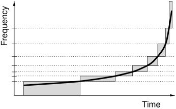
Figure 1 is a conceptual illustration of how the data contributes to the $\chi^{2}$ statistic. Because the chirp frequency rises monotonically, dividing the waveform into frequency bands is essentially equivalent to dividing it into time intervals. Each partial filter output $z_{l}(t_{c})$ is affected only by the data in its frequency band and time interval (the shaded boxes in the figure), with the appropriate time delay to relate it to the output of the full filter at the inferred coalescence time. Outside of this “chain” of boxes following the chirp, no other regions of the time-frequency plane affect the value of the $\chi^{2}$ statistic.

Triggers with $\chi^{2}$ values above some threshold are discarded. However, for large-amplitude signals, the $\chi^{2}$ statistic is highly sensitive to any small mismatch between the waveform and the template used for filtering, which is unavoidable given the discrete template bank used to perform the search. Therefore, a variable $\chi^{2}$ threshold, with an appropriate dependence on $\rho_{\rm max}$, is needed to avoid rejecting true inspiral signals which have very large amplitudes. For example, the LIGO S1 inspiral analysis [7] required $\chi^{2}$ to satisfy

$$\chi^{2}<40+0.15\;\rho_{\rm max}^{2}\;.$$ (6)

4 Inspiral event candidates from the LIGO S1 science run

Figure 2: Time series of (a) $\rho(t)$ and (b) $\chi^{2}(t)$ in the vicinity of the highest-amplitude inspiral event candidate found by the LIGO S1 search, on two different time scales. For comparison, (c) and (d) show the time series for a simulated inspiral signal added to fairly well-behaved detector noise from a different time during the S1 run.

The search for binary neutron star inspirals in LIGO S1 data [7] did not find any coincident “event candidates” with consistent signals in the two interferometers used in the analysis. Triggers from the individual interferometers (when a coincidence check was not possible) which exceeded the $\rho^{\ast}$ threshold and passed the $\chi^{2}$ test were considered event candidates for purposes of calculating an upper limit on the rate of inspirals in the Galaxy.

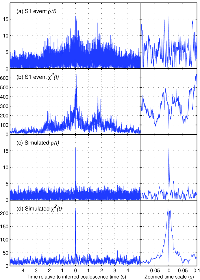
Follow-up examination of several event candidates with the largest SNRs revealed that they did not resemble true inspiral events. Plots (a) and (b) of figure 2 show the $\rho(t)$ and $\chi^{2}(t)$ time series for the event with the largest SNR, $15.9$, which was also shown in figure 5 of reference [7]. Both time series are larger on average, and more variable, for a period of several seconds around the inferred coalescence time reported by the search algorithm. (For comparison, the time series expected for a real inspiral signal in stationary detector noise are shown in figure 2 (c) and (d).) The trigger was generated when the $\chi^{2}$ happened to fluctuate down to a value below the threshold, which was 78 for this event according to equation (6). This particular event was found to have been due to a saturation of the photodiode which produces the data channel that was analyzed, but other large-SNR event candidates without obvious instrumental causes show similarly anomalous behavior in the time series. Nevertheless, the search algorithm used in the S1 inspiral analysis found this event candidate, and others, because it considered the values of $\rho$ and $\chi^{2}$ only at a single point in time.

5 Tests based on filter output history

Based on examining event candidates like the one shown in the previous section, we concluded that a test based on the filter output over a time interval, rather than just at a single point in time, should provide an effective way to reject events like these which are caused by non-stationary noise. In essence, we wanted to find a quantitative measure of the visually obvious difference between the data event and the simulated event in figure 2, some sort of check that the detector noise around the time of the trigger was consistent with the stationary noise assumed by the matched filter. Various approaches are possible; we decided to focus on simple tests using the $\rho(t)$ time series over a short interval just before the inferred coalescence time. We implemented a few potential tests by modifying the “findchirp” [14] inspiral search code in the LIGO/LSC Algorithm Library (LAL) [15] and studied the effectiveness of these tests on the event candidates found in the S1 data as well as on simulated events. Note that the computational cost of these tests is essentially zero, since the time series of the filter output is already available in memory.

We found that a good way to distinguish real inspiral signals from these triggers caused by non-stationarity is to count the number of “crossings”, $N_{c}$, in the half-second interval leading up to the inferred coalescence time, where a “crossing” is an instance of the $\rho(t)$ time series crossing over a threshold value, $\rho^{\times}$, in the up-going direction. (Every trigger has at least one crossing, as $\rho(t)$ rises to its peak value.) We initially chose $\rho^{\times}=6.5$, which yielded large values of $N_{c}$ for many of the large-SNR event candidates in the S1 data. Small-amplitude simulated events, like the one in figure 2(c), had just one or occasionally two crossings. However, we found that larger-amplitude simulated events often crossed this threshold several times. Figure 3

Figure 3: Time series of $\rho(t)$ for a simulated inspiral signal with very large amplitude. Detector noise, while present, is small on the scale shown. The “bumps” on either side of the main peak are due to real correlations between the matched filter and time-shifted signal waveforms.

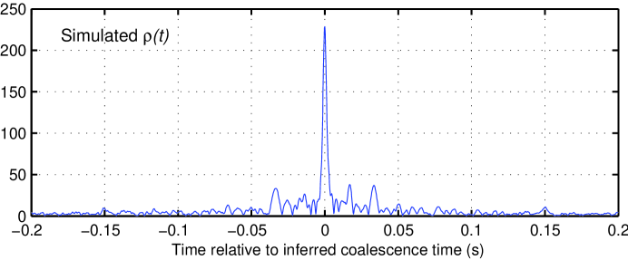
reveals the reason, showing the filter output for a simulated event with very large amplitude: even when filtered with an exactly matching template, the main $\rho(t)$ peak is accompanied by several additional “bumps” which far exceed $6.5$. These bumps are due to the autocorrelation of the waveform when time-shifted, and their exact shape will depend on $S_{n}(f)$ since it affects the filter (equation (1)). For the S1 data, we found that the height of these bumps relative to the peak was reasonably consistent for inspiral waveforms with various parameters, so we settled on a $\rho_{\rm max}$-dependent threshold of the form

$$\rho^{\times}=\sqrt{(6.5)^{2}+(\rho_{\rm max}/6)^{2}}\;.$$ (7)

Figure 4

Figure 4: Time series of $\rho(t)$ for: (a) the highest-amplitude inspiral event candidate found by the LIGO S1 search; (b) a simulated inspiral signal with the same value of $\rho_{\rm max}$; and (c) a simulated inspiral signal with a much larger $\rho_{\rm max}$. The two horizontal line segments in each plot indicates the half-second time interval for counting “crossings” with a fixed threshold of $\rho^{\times}=6.5$ (lower, thinner line in each plot) and with the $\rho_{\rm max}$-dependent threshold calculated according to equation (7) (upper, thicker line in each plot).

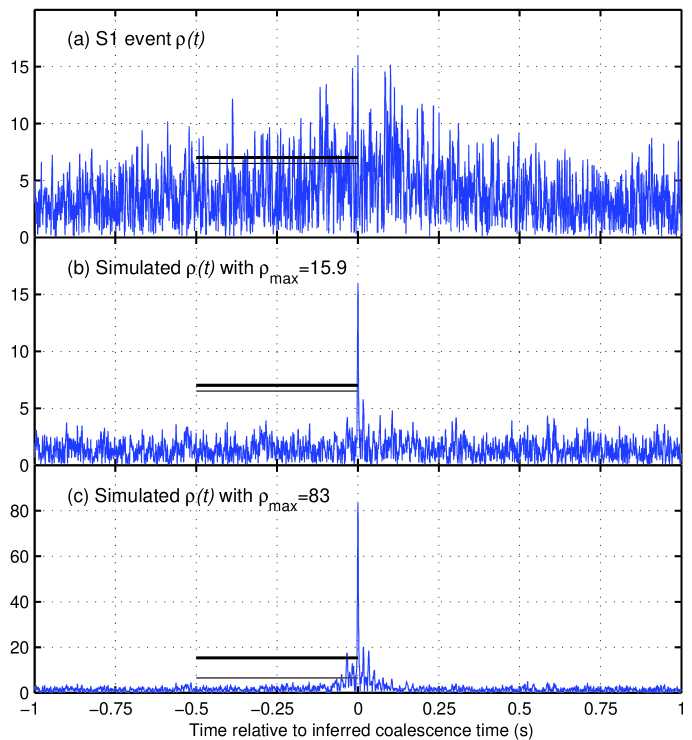
illustrates the application of this test to the loudest S1 event candidate as well as simulated inspiral events with small and large $\rho_{\rm max}$. The fixed threshold (thinner horizontal line in each plot) and the $\rho_{\rm max}$-dependent threshold (thicker horizontal line) are nearly the same for triggers with $\rho_{\rm max}<16$. For large-amplitude simulated events, the $\rho_{\rm max}$-dependent threshold is substantially higher and avoids most of the bumps in the $\rho(t)$ time series; $N_{c}$ is usually 1 or 2 for these simulated events.

6 Application to LIGO S1 data

Figure 5: Histograms of number of crossings for (a) data events found in the LIGO S1 search and (b) simulated inspiral signals from the population model used in that analysis [7].

Figure 6: Number of crossings vs. signal-to-noise ratio for data events found in the LIGO S1 search. The horizontal line indicates the requirement $N_{c}\leq 4$, which eliminates the 12 events with the largest values of SNR, as well as some events with smaller values of SNR.

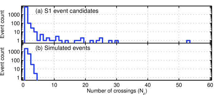
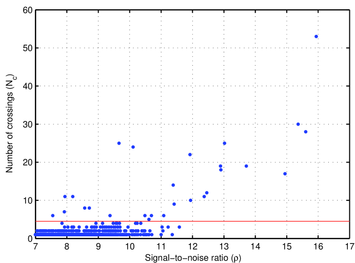
We re-analyzed the full S1 data set, calculating $N_{c}$ for each event candidate as described in the previous section. We also re-analyzed the set of simulated inspiral events generated from a population model of the Galaxy and Magellanic clouds, which was used to evaluate the efficiency of the search algorithm in the original analysis. Histograms of $N_{c}$ for both samples are shown in figure 5. None of the simulated events had more than four crossings, while a small but significant fraction of the data events had more than four. Figure 6 shows that the event candidates with the highest numbers of crossings are generally the ones with the largest values of SNR, which are the ones we particularly want to be able to reject. In fact, by requiring $N_{c}\leq 4$, we eliminate the 12 event candidates with the largest values of SNR.

This test was developed after the LIGO S1 analysis was finalized, so it is not reflected in the published result. In fact, the test was tuned specifically to eliminate the large-SNR event candidates in the S1 data sample, so it would, in principle, bias an upper limit analysis based on that data sample. Nevertheless, the ability of the test to cleanly distinguish between real and false inspiral events is very clear.

7 Summary and Discussion

We have proposed a new type of waveform consistency test for binary inspiral searches which uses the time history of the matched filter output and which is complementary to the standard $\chi^{2}$ test. A simple test of this type, tuned heuristically using the LIGO S1 data, was highly successful at eliminating large-SNR event candidates without introducing any measurable inefficiency for real inspiral signals. We believe that this technique will be valuable for future inspiral searches, although it will have to be tuned based on the nature of the non-stationarity in the detector noise. Within the context of the number-of-crossings test, a different time interval could be used, or the threshold could be chosen differently; it could even have some functional dependence on time relative to the inferred coalescence time. There are, of course, many alternative ways to derive a scalar statistic from the $\rho(t)$ and/or $\chi^{2}(t)$ time series, with various threshold or distribution tests. For instance, Guidi has proposed using the maximum value of the filter output time series, modified by subtracting the contribution expected from the putative signal, over a time interval before the inferred coalescence time [16]. The goal of any test of this type is to evaluate whether the detector noise in the vicinity of the trigger is consistent with the stationary noise assumed by the matched filter.

References

- [1] Cutler C and Flanagan É E 1994 Phys. Rev.D 49 2658–97
- [2] Balasubramanian R et al1996 Phys. Rev.D 53 3033–55
- [3] [] Balasubramanian R et al1996 Phys. Rev.D 54 1860 (erratum)
- [4] Buonanno A et al2003 Phys. Rev.D 67 024016
- [5] [] Buonanno A et al2003 Phys. Rev.D 67 104025
- [6] Abbott B et al2004 Nucl. Instrum. MethodsA 517 154–79
- [7] Abbott B et al2004 Phys. Rev.D in press
- [8] [] (Abbott B et al2003 Preprint gr-qc/0308069)
- [9] Droz S et al1999 Phys. Rev.D 59 124016
- [10] Allen B 2000 GRASP: a data analysis package for gravitational wave detection, version 1.9.8 manual pp 180–8
- [11] [] (URL http://www.lsc-group.phys.uwm.edu/~ballen/grasp-distribution)
- [12] Allen B et al1999 Phys. Rev. Lett.83 1498–1501
- [13] Tagoshi H et al2001 Phys. Rev.D 63 062001
- [14] Allen B et alin preparation
- [15] URL http://www.lsc-group.phys.uwm.edu/lal
- [16] Guidi G 2004 Class. Quantum Grav.submitted this issue