Arnowitt–Deser–Misner gravity with variable $G$ and $\Lambda$ and fixed point cosmologies from the renormalization group

Abstract

Models of gravity with variable $G$ and $\Lambda$ have acquired greater relevance after the recent evidence in favour of the Einstein theory being non-perturbatively renormalizable in the Weinberg sense. The present paper applies the Arnowitt–Deser–Misner (ADM) formalism to such a class of gravitational models. A modified action functional is then built which reduces to the Einstein–Hilbert action when $G$ is constant, and leads to a power-law growth of the scale factor for pure gravity and for a massless $\phi^{4}$ theory in a Universe with Robertson–Walker symmetry, in agreement with the recently developed fixed-point cosmology. Interestingly, the renormalization-group flow at the fixed point is found to be compatible with a Lagrangian description of the running quantities $G$ and $\Lambda$. PACS: 04.20.Fy, 04.60.-m, 11.10.Hi, 98.80.Cq

I Introduction

Recent studies support the idea that the Newton constant $G$ and the cosmological constant $\Lambda$ are actually spacetime functions by virtue of quantum fluctuations of the background metric [1] ; [2] ; [3] ; [4] . Their behaviour is ruled by the renormalization group (hereafter RG) equations for a Wilson-type Einstein-Hilbert action where $\sqrt{g}R$ and $\sqrt{g}$ become relevant operators in the neighbourhood of a non-perturbative ultraviolet fixed point in four dimensions [5] . The theory is thus asymptotically safe in the Weinberg sense [6] because the continuum limit is recovered at this new ultraviolet fixed point. In other words, the theory is non-perturbatively renormalizable [7] ; [8] ; [9] ; [10] .

Within this framework, the basic ingredient to promote $G$ and $\Lambda$ to the role of spacetime functions is the renormalization group improvement, a standard device in particle physics in order to add, for instance, the dominant quantum corrections to the Born approximation of a scattering cross section. The basic idea of this approach is similar to the renormalization group based derivation of the Uehling correction to the Coulomb potential in massless QED [11] . The “RG improved” Einstein equations can thus be obtained by replacing $G\to G(k)$, $\Lambda\to\Lambda(k)$, where $k$ is the running mass scale which should be identified with the inverse of cosmological time in a homogeneous and isotropic Universe, $k\propto 1/t$ as discussed in Refs. [3] ; [4] , or with inverse of the proper distance $k\propto 1/d(P)$ of a freely falling observer in a Schwarzschild background [1] ; [2] .

In this way the RG running gives rise to a dynamically evolving, spacetime dependent $G$ and $\Lambda$. The improvement of Einstein’s equations can then be based upon any RG trajectory $k\mapsto(G(k),\Lambda(k))$ obtained as an (approximate) solution to the exact RG equation of (quantum) Einstein-Gravity. Within this framework it has been shown that the renormalization group derived cosmologies provide a solution to the horizon and flatness problem of standard cosmology without any inflationary mechanism. They represent also a promising model of dark energy in the late Universe [12] . A similar approach has also been discussed in Ref. [13] , where the RG equation arises from the matter field fluctuations.

In comparison to earlier work [14] ; [15] ; [16] ; [17] ; [18] on cosmologies with a time dependent $G$, $\Lambda$ and possibly fine structure constant $\alpha$ the new feature of these RG derived cosmologies is that the time dependence of $G$ and $\Lambda$ is a secondary effect which results from a more fundamental scale dependence. In a typical Brans-Dicke type theory the dynamics of the Brans-Dicke field $\omega=1/G$ is governed by a standard local Lagrangian with a kinetic term $\propto(\partial_{\mu}\omega)^{2}$. In this approach there is no simple Lagrangian description of the $G$-dynamics a priori. It rather arises from an RG equation for $G(k)$ and a cutoff identification $k=k(x^{\mu})$. From the point of view of the gravitational field equations, $G(x^{\mu})$ has the status of an external scalar field whose evolution is engendered by the RG equations. It is nevertheless interesting to notice that a dynamically evolving cosmological constant and asymptotically free gravitational interaction also appear in very general scalar-tensor cosmologies [19] ; [20] .

In general, the RG equations do not admit a gradient flow representation and it is not clear how to embed the RG behaviour into a Lagrangian formalism. This problem has been widely discussed in Ref. [21] where a consistent RG improvement of the Einstein-Hilbert action has been proposed at the level of the four-dimensional Lagrangian.

Instead, the relevant question we would like to study in this paper is how to achieve a modification of the standard ADM Lagrangian where $G$ and $\Lambda$ are dynamical variables according to a prescribed renormalized trajectory (see Ref. [22] for a first attempt in this direction). The simplest non-trivial renormalization group trajectory is represented by the scaling law near a fixed point for which

$$G(x^{\mu})\;\Lambda(x^{\mu})={\rm const},$$ (1)

and we shall use the simple relation (1) to constrain the possible dynamics.

Indeed, a theory with an independent dynamical $G$ is known to be equivalent to metric-scalar gravity already at classical level. In particular, it can be reduced to canonical form with the standard expression of the kinetic term for the scalar by a conformal rescaling of the metric (see a discussion of this point in Ref. [23] ). At this stage, a theory where Lambda is an independent dynamical variable meets serious problems, in agreement with what we find below.

Following the fixed-point relation as implemented in Eq. (1), in this paper we thus discuss a dynamics according to which $\Lambda$ depends on $G$ which is, in turn, a function of position and time. If $\Lambda$ and $G$ were instead taken to be independent functions of position and time, the primary constraint of vanishing conjugate momentum to $\Lambda$ would lead to a secondary constraint which is very pathological, and details will be given later in Sec. II to avoid logical jumps.

In Sec. II we introduce and motivate a modified action functional for theories of gravitation with variable $G$ and $\Lambda$. Such a result is applied, in Sec. III, to pure gravity and to gravity coupled to a massless self-interacting scalar field in a Universe with Robertson–Walker (hereafter RW) symmetry. Concluding remarks and open problems are presented in Sec. IV, while the full Hamiltonian analysis is performed in the appendix.

II Modified action functional

According to the ADM treatment of space-time geometry, we now assume that the space-time manifold $(M,g)$ is topologically $\Sigma\times R$ and is foliated by a family of spacelike hypersurfaces $\Sigma_{t}$ all diffeomorphic to $\Sigma$. The metric is then locally cast in the ADM form

$$g=-(N^{2}-N_{i}N^{i})dt\otimes dt+N_{i}(dx^{i}\otimes dt+dt\otimes dx^{i})+h_{ij}dx^{i}\otimes dx^{j},$$ (2)

where $N$ is the lapse function and $N^{i}$ are the components of the shift vector [24] . To obtain the ADM form of the action, one has to consider the induced Riemannian metric $h_{ij}dx^{i}\otimes dx^{j}$ on $\Sigma$, the extrinsic-curvature tensor $K_{ij}={1\over 2N}\Bigr{(}-h_{ij,0}+2N_{(i\mid j)}\Bigr{)}$ of $\Sigma$ (hereafter $h_{ij,0}\equiv{\partial h_{ij}\over\partial t}$, and similarly for $N,N_{i}$ and $G$), and add a suitable boundary term to the Einstein–Hilbert action, which is necessary to ensure stationarity of the full action functional in the Hamilton variational problem [25] . More precisely, the fundamental identity in Ref. [26] (hereafter $h\equiv{\rm det}\;h_{ij},K\equiv K_{\;i}^{i}$, and ${}^{(3)}R$ is the scalar curvature of $\Sigma$)

$$\sqrt{-g}\;{}^{(4)}R=N\sqrt{h}(K_{ij}K^{ij}-K^{2}+{}^{(3)}R)-2(K\sqrt{h})_{,0}+2f_{\;,i}^{i},$$ (3)

where

$$f^{i}\equiv\sqrt{h}\Bigr{(}KN^{i}-h^{ij}N_{,j}\Bigr{)},$$ (4)

suggests using the Leibniz rule to express

$${1\over G}(K\sqrt{h})_{,0}={G_{,0}\over G^{2}}K\sqrt{h}+\left({K\sqrt{h}\over G}\right)_{,0},$$ (5)

$${1\over G}{\partial f^{i}\over\partial x^{i}}={G_{,i}\over G^{2}}f^{i}+{\partial\over\partial x^{i}}\left({f^{i}\over G}\right),$$ (6)

so that division by $16\pi G$ in the integrand of the Einstein-Hilbert action yields the Lagrangian (the $c^{4}$ factor in the numerator is set to $1$ with our choice of units)

$$L={1\over 16\pi}\int\left[{N\sqrt{h}\over G}(K_{ij}K^{ij}-K^{2}+{}^{(3)}R-2\Lambda)-2{G_{,0}\over G^{2}}K\sqrt{h}+2{G_{,i}f^{i}\over G^{2}}\right]d^{3}x,$$ (7)

after adding to the action functional the boundary term (cf. Ref. [25] )

$$I_{\Sigma}={1\over 8\pi}\int_{\Sigma}{K\sqrt{h}\over G}d^{3}x,$$

and assuming that $\Sigma$ is a closed manifold (so that the total spatial divergence of ${f^{i}\over G}$ resulting from (3) and (6) yields vanishing contribution, having taken $\partial\Sigma=\emptyset$).

The Lagrangian (7), however, suffers from a serious drawback, because the resulting momentum conjugate to the three-metric reads as

$$p^{ij}\equiv{\delta L\over\delta h_{ij,0}}=-{\sqrt{h}\over 16\pi G}(K^{ij}-h^{ij}K)+{\sqrt{h}\over 16\pi G}{h^{ij}\over NG}(G_{,0}-G_{,k}N^{k}).$$ (8)

This would yield, in turn, a Hamiltonian containing a term quadratic in $G_{,0}$ (since $K^{ij}$ depends, among the others, on $p^{ij}$ and on $G_{,0}h^{ij}$), despite the fact that (7) is only linear in $G_{,0}$ when expressed in terms of first and second fundamental forms. There is therefore a worrying lack of equivalence between $K^{ij}$ and $p^{ij}$.

We thus decide to include a “bulk” contribution in order to cancel the effect of $G_{,0}$ and $G_{,i}$ in Eq. (7) by writing

$$I\equiv{1\over 16\pi}\int_{M}{({}^{(4)}R-2\Lambda)\over G({\vec{x}},t)}\sqrt{-g}\;d^{4}x+{1\over 8\pi}\int_{M}{(K\sqrt{h})_{,0}\over G({\vec{x}},t)}d^{4}x-{1\over 8\pi}\int_{M}{f_{\;,i}^{i}\over G({\vec{x}},t)}d^{4}x,$$ (9)

as a starting action defining a gravitational theory with variable $G$ and $\Lambda$, where the added terms in Eq. (9) have integrands which are not four-dimensional total divergences. More precisely, upon division by $16\pi G$ in the integrand of the Einstein–Hilbert term (first integral in Eq. (9)), the second and third integral in Eq. (9) cancel the effect of $-2(K\sqrt{h})_{,0}$ and $2f_{\;,i}^{i}$ in Eq. (3), respectively. The resulting Lagrangian density belongs to the general family depending only on fields and their first derivatives, which is the standard assumption in local field theory. It should also be noticed that if $G$ were constant, the second integral on the right-hand side of (9) would reduce to the York–Gibbons–Hawking boundary term [25] ; [27]

$${1\over 8\pi G}\int_{\Sigma}K\sqrt{h}\;d^{3}x.$$

Moreover, for a constant $G$, the third integral on the right-hand side would reduce to

$$-{1\over 8\pi G}\int dt\int_{\partial\Sigma}f^{i}n_{i}d^{2}x,$$

which vanishes if $\Sigma$ is the smooth boundary of $M$ (since then $\partial\Sigma=\partial\partial M=0$).

In other words, on renormalization-group improving the gravitational Lagrangian in the ADM approach, one might think that $G$ and $\Lambda$ have the status of given external field, whose evolution is in principle dictated by the RG flow equation. However, it is also interesting to understand whether one can generalize the standard ADM Lagrangian in order to consider $G$ as a dynamical field and investigate which dynamics is consistent with the RG approach. In this spirit we eventually consider the following general ADM Lagrangian:

$$L={1\over 16\pi}\int\left[{N\sqrt{h}\over G}(K_{ij}K^{ij}-K^{2}+{}^{(3)}R-2\Lambda)\right]d^{3}x+L_{\rm int}+L_{\rm matter},$$ (10)

where the first term has the same functional form as the Lagrangian of ADM general relativity (but with $G$ and $\Lambda$ promoted to mutually related dynamical variables), $L_{\rm int}$ is an interaction term of a kinetic type which, for dimensional reasons, must be of the form (the coefficient $16\pi$ is introduced for later convenience)

$$L_{\rm int}=-{\mu\over 16\pi}\int{g^{\rho\sigma}G_{;\rho}G_{;\sigma}\over G^{3}}\;\sqrt{-g}\;d^{3}x$$ (11)

$$= {\mu\over 16\pi}\int{N\sqrt{h}\over G^{3}}\left[N^{-2}(G_{,0})^{2}-2{N^{i}\over N^{2}}G_{,0}G_{,i}-\left(h^{ij}-{N^{i}N^{j}\over N^{2}}\right)G_{,i}G_{,j}\right]d^{3}x,$$

$\mu$ being the interaction parameter, and the occurrence of lapse and shift being the effect of ADM coordinates in writing the integration measure for the action and the space-time metric. $L_{\rm matter}$ is the “matter” Lagrangian that we shall consider as given by a self-interacting scalar field. The first line of Eq. (11) stresses that we start from an action which is invariant under four-dimensional diffeomorphisms, although eventually re-expressed in ADM variables (second line of Eq. (11)). It should be emphasized that there are no observational constraints on the term $L_{\rm int}$ in Eq. (11), since we are considering modifications of general relativity which only occur in the very early universe at about the Planck scale. Experimental verifications of our model, although clearly desirable, are beyond the aims of the present work.

Note that, if $\Lambda$ were a variable function, but independent of $G$, the primary constraint of vanishing conjugate momentum to $\Lambda$ would lead to the secondary constraint ${N\sqrt{h}/(8\pi G)}$, which would vanish on the constraint manifold. This is very pathological, because it implies that either the lapse vanishes or the induced three-metric on the surfaces of constant time has vanishing determinant. Neither of these alternatives seems acceptable in a viable space-time model.

We have also found that, if $\mu$ is instead set to zero, one obtains the additional primary constraint $\pi_{G}\approx 0$ (the weak-equality symbol $\approx$ is used for equations which only hold on the constraint surface [28] ; [29] ), and the resulting dynamical system, with its evolution and constraint equations, is incompatible with a dynamical evolution of the scale factor, leading only to an Einstein-Universe type of solution. For this reason we can conclude that the generalized Lagrangian described in Eq. (10) represents a minimal viable modification of the standard gravitational Lagrangian which would lead to a dynamical $G$.

III RW symmetry

In this section we study a class of scalar field cosmologies within our new modified Lagrangian framework. On using the ADM formalism, we take a scalar-field Lagrangian [30]

$$L_{m}\equiv\int{N\sqrt{h}\over 2}\left[N^{-2}(\phi_{,0})^{2}-2{N^{i}\over N^{2}}\phi_{,0}\phi_{,i}-\left(h^{ij}-{N^{i}N^{j}\over N^{2}}\right)\phi_{,i}\phi_{,j}-2V(\phi)\right]d^{3}x,$$ (12)

where the potential $V(\phi)$ is, for the time being, un-determined, and $g^{00}$ is negative with our convention for the space-time metric.

We focus, hereafter, on cosmological models with RW symmetry. Strictly speaking, such a name can be criticized, since we are no longer studying general relativity, nor are we simply RG-improving the Einstein equations. Nevertheless, we will find that spatially homogeneous and isotropic cosmological models of the RW class can still be achieved. In such models with lapse function $N=1$, the full Lagrangian, including scalar field, reads as (here ${\cal K}=1,0,-1$ for a closed, spatially flat or open universe, respectively)

$$L={a^{3}\over 16\pi G}\left(-6{{\dot{a}}^{2}\over a^{2}}+{6{\cal K}\over a^{2}}-2\Lambda\right)+{\mu\over 16\pi}{a^{3}{\dot{G}}^{2}\over G^{3}}+a^{3}\left({{\dot{\phi}}^{2}\over 2}-V(\phi)\right),$$ (13)

where hereafter we revert to dots, for simplicity, to denote derivatives with respect to $t$. Thus, the resulting second-order Euler–Lagrange evolution equations for $a,G$ and $\phi$ are

$${{\ddot{a}}\over a}+{1\over 2}{{\dot{a}}^{2}\over a^{2}}+{{\cal K}\over 2a^{2}}-{\Lambda\over 2}-{{\dot{a}}\over a}{{\dot{G}}\over G}+{\mu\over 4}{{\dot{G}}^{2}\over G^{2}}+4\pi G\left({{\dot{\phi}}^{2}\over 2}-V(\phi)\right)=0,$$ (14)

$$\mu{\ddot{G}}-{3\over 2}\mu{{\dot{G}}^{2}\over G}+3\mu{\dot{a}\over a}{\dot{G}}+{G\over 2}\left(-6{{\dot{a}}^{2}\over a^{2}}+6{{\cal K}\over a^{2}}-2\Lambda+2G{d\Lambda\over dG}\right)=0,$$ (15)

$${\ddot{\phi}}+3{{\dot{a}}\over a}{\dot{\phi}}+{dV\over d\phi}=0.$$ (16)

Moreover, since the Lagrangian (10) is independent of time derivatives of the lapse, one has the primary constraint of vanishing conjugate momentum to $N$ (see Eq. (A1) of the appendix). The preservation in time of such a primary constraint yields, for our Lagrangian generated from the assumption of RW symmetry, the constraint equation (cf. Eqs. (A8) and (A10) of the appendix)

$$\left({{\dot{a}}\over a}\right)^{2}+{{\cal K}\over a^{2}}-{\Lambda\over 3}-{\mu\over 6}{{\dot{G}}^{2}\over G^{2}}-{8\pi G\over 3}\left({{\dot{\phi}}^{2}\over 2}+V(\phi)\right)\approx 0.$$ (17)

This latter equation can be rewritten in a more familiar form by introducing vacuum, matter, $G$ energy densities, respectively, as follows:

$$\rho_{\Lambda}\equiv{\Lambda(t)\over 8\pi G(t)},\;\;\;\;\rho_{\phi}\equiv\dot{\phi}^{2}/2+V(\phi),\;\;\;\;\;\;\ \rho_{G}\equiv{\mu\over 16\pi}{\dot{G}^{2}\over G^{3}},$$ (18)

so that the total energy density is given by $\rho=\rho_{\Lambda}+\rho_{\phi}+\rho_{G}$, and Eq. (17) reads as

$$\frac{{\cal K}}{a^{2}}=\Big{(}\frac{\dot{a}}{a}\Big{)}^{2}(\Omega-1),$$ (19)

where $\Omega\equiv\rho/\rho_{\rm cr}$, and the critical density is defined as usual by

$$\rho_{\rm cr}\equiv{3\over 8\pi G(t)}\left({\dot{a}\over a}\right)^{2}.$$ (20)

Although it would be interesting to discuss the general properties of the above system, our main motivation is to use RG arguments to select a particular class of possible solutions. In fact the RG evolution of $G$ and $\Lambda$ near a fixed point strongly constrains the possible solutions. More precisely, it is assumed that there exists a fundamental scale dependence of Newton’s parameter which is governed by an exact RG equation for a Wilsonian effective action whose precise nature need not be specified here. At a typical length scale $\ell$ or mass scale $k=\ell^{-1}$ those “constants” assume the values $G(k)$ and $\Lambda(k)$, respectively. On trying to “RG-improve” $G$ and $\Lambda$ the crucial step is the identification of the scale $\ell$ or $k$ which is relevant for the situation under consideration. In cosmology, the postulate of homogeneity and isotropy implies that $k$ can only depend on the cosmological time, so that the scale dependence is turned into a time dependence:

$$G(t)\equiv G(k=k(t)),\;\;\;\Lambda(t)\equiv\Lambda(k=k(t)).$$ (21)

In principle the time dependence of $k$ can be either explicit or implicit via the scale factor: $k=k(t,a(t),\dot{a}(t),\ddot{a}(t),\cdots)$. In Refs. [3] ; [4] detailed arguments are given as to why the explicit purely temporal dependence is

$$k(t)={\xi}/{t},$$ (22)

$\xi$ being a positive constant. In a nutshell, the argument is that, when the age of the Universe is $t$, no (quantum) fluctuation with a frequency smaller than $1/t$ can have played any role as yet. Hence the integrating-out of modes (“coarse graining”) which underlies the Wilson renormalization group should be stopped at $k\approx 1/t$. In the neighbourhood of a fixed point $(g_{\star},\lambda_{\star})$ the evolution of the dimensionful $G$ and $\Lambda$ is approximately given by

$$G(k)=\frac{g_{\star}}{k^{2}},\;\;\;\;\Lambda(k)=\lambda_{\star}\;k^{2}.$$ (23)

From (23) with (22) we obtain the time-dependent Newton parameter and cosmological term:

$$G(t)=g_{\star}\xi^{-2}\;t^{2},\;\;\;\;\Lambda(t)=\frac{\lambda_{\star}\xi^{2}}{t^{2}}.$$ (24)

We should mention, however, that there is another choice in the literature, where $G$ and $\Lambda$ are related, through the renormalization group, to the Hubble parameter $H$. Since $H$ is a function of the metric which is directly related to the energy of gravitational quanta for the cosmological setting, such a choice has been viewed to fit more naturally with the RG approach by some authors [31] .

The power laws (24) are valid for $t\rightarrow 0$ (UV case, Early Universe) or for $t\rightarrow\infty$ (IR case, Late Universe), respectively. If we use these functions $G(t)$ and $\Lambda(t)$ in the dynamical system its solution gives us the scale factor $a(t)$ and the density $\rho_{\phi}(t)$ of the “RG improved scalar field cosmology”. Let us now discuss some solutions.

III.1 Pure gravity

Unlike models where only the Einstein equations are RG-improved, our framework allows for a non-trivial dynamics of the scale factor even in the absence of coupling to a matter field. To appreciate this point, consider first the case when no scalar field exists, so that Eq. (16) should not be considered. The relation (23) suggests looking for power-law solutions of the type

$$a(t)=A\;t^{\alpha},\;\;\;\;\;G(t)=g_{\star}\xi^{-2}t^{2},\;\;\;\;\Lambda(t)=\lambda_{\star}\xi^{2}t^{-2},$$ (25)

and separately consider the ${\cal K}=0$ and ${\cal K}=\pm 1$ case. For ${\cal K}=0$ we obtain that $A$ is an un-determined factor, while

$$\mu_{\pm}=\frac{1}{4}(3\pm\sqrt{9+12\;\xi^{2}\lambda_{\star}}),\;\;\;\;\alpha_{\pm}=\frac{1}{6}(3\pm\sqrt{9+12\;\xi^{2}\lambda_{\star}}),$$ (26)

which implies a power-law inflation for the “$+$” solution, $\alpha_{+}$ being larger than $1$ if $\lambda_{\star}>0$, and a possible solution of the horizon problem. Note that the first equality is a relation between coupling constants which has to be satisfied, while the second simply relates the value of $\alpha$ with the product $\xi^{2}\lambda_{\star}$. Since $\xi$ is not determined, $\alpha_{+}$ can be made arbitrarily large. Moreover, both $\Omega_{G}$ and $\Omega_{\Lambda}$ are constant, since

$$\Omega_{G}=1-\Omega_{\Lambda}=\frac{6}{3\pm\sqrt{9+12\;\xi^{2}\lambda_{\star}}}.$$ (27)

If ${\cal K}=\pm 1$ we find instead $\alpha=1$ and

$$\mu=\frac{1}{4}(6+\xi^{2}\lambda_{\star}),\;\;\;\;\;\;\;\frac{{\cal K}}{A^{2}}=\frac{\xi^{2}\lambda_{\star}}{2},$$ (28)

where, as before, the former equation relates the values of the coupling constants, while the latter is a consistency relation. In particular we see that, if ${\cal K}=-1$, then $\lambda_{\star}$ must be negative.

In both cases (i.e. ${\cal K}=\pm 1$), $\Omega_{\Lambda}$ and $\Omega_{G}$ are constant with

$$\Omega_{\Lambda}=\frac{2{\cal K}}{3A^{2}},\;\;\;\;\;\Omega_{G}=1+\frac{{\cal K}}{3A^{2}}.$$ (29)

III.2 Inclusion of a scalar field

Here we consider the contribution of a scalar field with a self-interacting potential of the type

$$V(\phi)=\frac{\zeta}{4!}\phi^{4},$$ (30)

with the ansatz (25) for $a,G,\Lambda$, and $\phi=\phi_{0}t^{-\beta}$ for the scalar field. The Klein–Gordon equation of motion (16) then yields $\beta=1$ and

$$\phi_{0}=\pm\sqrt{\frac{6(3\alpha-2)}{\zeta}},$$ (31)

which implies $\alpha>2/3$ so as to have a real scalar field. We then find, if ${\cal K}=0$,

$$\alpha_{\pm}=\mu\pm\sqrt{\mu^{2}-\frac{4\mu}{3}-\frac{2\xi^{2}\lambda_{\star}}{3}},$$ (32)

$$\zeta_{\pm}=\frac{24g_{\star}\pi[3\xi^{2}\lambda_{\star}-3\mu^{2}+5\mu\pm(1-\mu)\sqrt{3\mu(3\mu-4)-6\xi^{2}\lambda_{\star}}]}{\xi^{2}(3\xi^{2}\lambda_{\star}+2(3-2\mu)\mu)},$$ (33)

where (33) is a consistency relation, (32) determines the value of $\alpha$, and a reality condition for $\xi^{2}\lambda_{\star}$ is given by $(3\xi^{2}\lambda_{\star}+2(3-2\mu)\mu)>0$. It is not difficult to see that there are physically interesting solutions with power-law inflation if $\mu$ is large enough and positive, and $\xi$ is positive. A plot of the behaviour of $\alpha$ and $\zeta$ as a function of $\mu$ and $\xi$ is depicted in Figs. (1) and (2), respectively, where the fixed-point values $g_{\star}=0.31$ and $\lambda_{\star}=0.35$ have been calculated in Ref. [32] for a self-interacting scalar field in Einstein–Hilbert gravity.

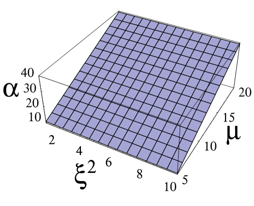
Figure 1: The exponent $\alpha$ as a function of $\mu$ and $\xi$ for the fixed-point values $g_{\star}=0.31$ and $\lambda_{\star}=0.35$ evaluated from the RG equation for a scalar field.

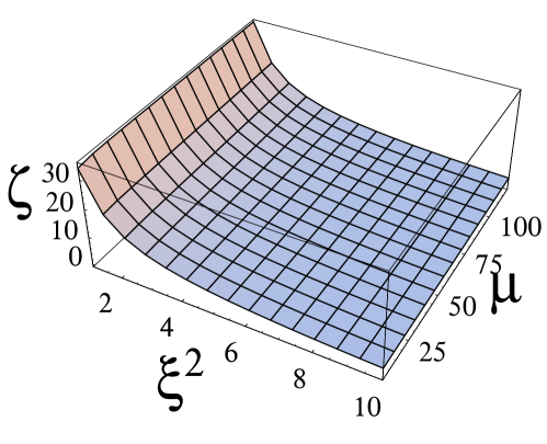
Figure 2: The self-interaction coupling $\zeta$ as a function of $\mu$ and $\xi$ for the fixed-point values $g_{\star}=0.31$ and $\lambda_{\star}=0.35$ evaluated from the RG equation for a scalar field.

If instead ${\cal K}=\pm 1$ the only solution is for $\alpha=1,\beta=1,$ and we get the consistency conditions

$$\mu=-\frac{9\pi\xi^{-2}g_{\star}}{\zeta}+\frac{1}{4}(6+\xi^{2}\lambda_{\star}),\;\;\;\;\;\;\frac{\cal K}{A^{2}}=\frac{6\pi\xi^{-2}g_{\star}}{\zeta}+{\xi^{2}\lambda_{\star}\over 2},\;\;\;\;\;\phi_{0}=\pm\sqrt{\frac{6}{\zeta}}.$$ (34)

For all cases, ${\cal K}=0$ and ${\cal K}\pm 1$, $\Omega_{G}$ and $\Omega_{\Lambda}$ take constant values.

IV Concluding remarks

The Lagrangian formulation of theories of gravity with variable Newton parameter has been considered both in classical [33] and in quantum theory [34] by a number of authors, while the effective average action and renormalizability of non-perturbative quantum gravity had been studied also in Refs. [35] ; [36] .

First, within the framework of relativistic theories of gravity with variable $G$ and $\Lambda$, we have arrived at the ADM Lagrangian (10), with coupling to a massless self-interacting scalar field as in Sec. III. Second, we have shown that, although the RG evolution is not derivable in general from a Hamiltonian dynamics, the RG flow at the fixed point is consistent with a Lagrangian description of the basic running quantities $G$ and $\Lambda$ in a RW universe provided that we modify the standard Lagrangian for gravity by adding new terms which preserve the standard form of momenta conjugate to the three-metric and ensure a well-posed Hamilton variational problem. We only exploit the scaling of scale factor, scalar field, $G$ and $\Lambda$ at the fixed point, which is universal (in the sense of statistical mechanics), and find that the desired fixed-point scaling actually exists even when the Lagrangian is allowed to rule the behaviour of the Newton parameter.

Third, we have presented explicit solutions for pure gravity and a self-interacting scalar field coupled to gravity in a RW Universe (see comments in Sec. III), finding a class of power-law inflationary models which solve the horizon problem of the cosmological standard model and can be used to test against observation a fixed-point cosmology inspired by the renormalization group but derived from a Lagrangian.

A challenging open problem is now the development of cosmological perturbation theory starting from Lagrangians as in Eq. (10). This could tell us whether formation of structure in the early universe can also be accommodated within the framework of a Wilson-type [37] formulation of quantum gravity.

Appendix A Hamiltonian analysis

Our generalized framework with Lagrangian (10) engenders the familiar primary constraints of general relativity, i.e.

$$\pi_{N}\equiv{\delta L\over\delta N_{,0}}\approx 0,$$ (35)

$$\pi^{i}\equiv{\delta L\over\delta{N_{i}}_{,0}}\approx 0,$$ (36)

with corresponding canonical Hamiltonian (for simplicity, we first consider the pure gravity case)

$$H\equiv\int\Bigr{(}\pi_{N}N_{,0}+\pi^{i}{N_{i}}_{,0}+\pi^{ij}h_{ij,0}+\pi_{G}G_{,0}\Bigr{)}d^{3}x-L,$$ (37)

where

$$\pi^{ij}\equiv{\delta L\over\delta h_{ij,0}}=-{\sqrt{h}\over 16\pi G}(K^{ij}-h^{ij}K),$$ (38)

$$\pi_{G}\equiv{\delta L\over\delta G_{,0}}={\mu\sqrt{h}\over 8\pi NG^{3}}\Bigr{(}G_{,0}-G_{,i}N^{i}\Bigr{)}.$$ (39)

The resulting effective Hamiltonian (i.e. the canonical Hamiltonian plus a linear combination of primary constraints [28] ; [29] ) can be cast in the form

$${\widetilde{H}}\equiv\int\Bigr{(}N{\cal H}_{0}+N_{i}{\cal H}^{i}+\nu_{N}\pi_{N}+\nu_{i}\pi^{i}\Bigr{)}d^{3}x,$$ (40)

where $\nu_{N}$ and $\nu_{i}$ are Lagrange multipliers for primary constraints, while ${\cal H}_{0}$ and ${\cal H}^{i}$ are the secondary constraints obtained by preserving $\pi_{N}$ and $\pi^{i}$, respectively. On defining the DeWitt (super-)metric on the space of Riemannian metrics on $\Sigma$ [26] :

$$G_{ijkl}\equiv{1\over 2\sqrt{h}}(h_{ik}h_{jl}+h_{il}h_{jk}-h_{ij}h_{kl}),$$ (41)

one has

$${\cal H}_{0}\equiv(16\pi G)G_{ijkl}\pi^{ij}\pi^{kl}-{\sqrt{h}\over 16\pi G}{}^{(3)}R+{\sqrt{h}\over 8\pi}{\Lambda(G)\over G}+{4\pi G^{3}\over\mu\sqrt{h}}\pi_{G}^{2}+{\mu\sqrt{h}\over 16\pi G^{3}}h^{ij}G_{,i}G_{,j},$$ (42)

$${\cal H}^{i}\equiv-2\pi_{\;\;\;\mid j}^{ij}+h^{ij}G_{,j}\pi_{G}.$$ (43)

When gravity is coupled to an external scalar field ruled by the Lagrangian (12), the secondary constraints read as

$${\widetilde{\cal H}}_{0}\equiv{\cal H}_{0}+{\sqrt{h}\over 2}\left[{\pi_{\phi}^{2}\over h}+h^{ij}\phi_{,i}\phi_{,j}+2V(\phi)\right],$$ (44)

$${\widetilde{\cal H}}^{i}\equiv{\cal H}^{i}+h^{ij}\phi_{,j}\pi_{\phi}.$$ (45)

In the cosmological models of Sec. III, the Lagrangian in Eq. (13) gives rise to the Hamiltonian (with $\pi_{a}$ the momentum conjugate to the scale factor)

$$H=-{2\over 3}{\pi G\over a}\pi_{a}^{2}+{4\pi G^{3}\over\mu a^{3}}\pi_{G}^{2}+{\pi_{\phi}^{2}\over 2a^{3}}-{3{\cal K}a\over 8\pi G}+{\Lambda a^{3}\over 8\pi G}+a^{3}V(\phi).$$ (46)

The resulting Hamilton equations of motion are

$${\dot{a}}=\left\{a,H\right\}=-{4\pi G\over 3a}\pi_{a},$$ (47)

$${\dot{G}}=\left\{G,H\right\}={8\pi G^{3}\over\mu a^{3}}\pi_{G},$$ (48)

$${\dot{\phi}}=\left\{\phi,H\right\}={\pi_{\phi}\over a^{3}},$$ (49)

$${\dot{\pi}}_{a}=\left\{\pi_{a},H\right\}=-{2\over 3}{\pi G\over a^{2}}\pi_{a}^{2}+{12\pi G^{3}\over\mu a^{4}}\pi_{G}^{2}+{3\pi_{\phi}^{2}\over 2a^{4}}+{3{\cal K}\over 8\pi G}-{3\Lambda a^{2}\over 8\pi G}-3a^{2}V(\phi),$$ (50)

$${\dot{\pi}}_{G}=\left\{\pi_{G},H\right\}={2\over 3}{\pi\over a}\pi_{a}^{2}-{12\pi G^{2}\over\mu a^{3}}\pi_{G}^{2}-{3{\cal K}a\over 8\pi G^{2}}+{\Lambda a^{3}\over 8\pi G^{2}}-{a^{3}\over 8\pi G}{d\Lambda\over dG},$$ (51)

$${\dot{\pi}}_{\phi}=\left\{\pi_{\phi},H\right\}=-a^{3}{dV\over d\phi}.$$ (52)

Equations (A13)–(A18) can be solved for given initial conditions $a(0),G(0),\phi(0),\pi_{a}(0),\pi_{G}(0),\pi_{\phi}(0)$, provided that such an initial data set satisfies the Hamiltonian constraint $H\approx 0$ (cf. Eq. (17)).

Full agreement with the Euler–Lagrange equations (14)–(16) is proved on taking the time derivative of Eqs. (A13)–(A15) and then re-expressing the momenta $\pi_{a},\pi_{G},\pi_{\phi}$ and their first derivatives from Eqs. (A13)–(A18). For example, Eq. (A13) implies that

$${\ddot{a}}=-{4\pi\over 3}\left({{\dot{G}}\over a}-G{{\dot{a}}\over a^{2}}\right)\pi_{a}-{4\pi\over 3}{G\over a}{\dot{\pi}}_{a},$$

and the insertion of Eqs. (A13) and (A16) yields eventually Eq. (14) of Sec. III.