Inflationary Cosmology and Quantization Ambiguities
in Semi-Classical Loop Quantum Gravity

Abstract

In loop quantum gravity, modifications to the geometrical density cause a self-interacting scalar field to accelerate away from a minimum of its potential. In principle, this mechanism can generate the conditions that subsequently lead to slow-roll inflation. The consequences for this mechanism of various quantization ambiguities arising within loop quantum cosmology are considered. For the case of a quadratic potential, it is found that some quantization procedures are more likely to generate a phase of slow–roll inflation. In general, however, loop quantum cosmology is robust to ambiguities in the quantization and extends the range of initial conditions for inflation.

I Introduction

Loop quantum gravity (LQG) or quantum geometry is at present the main background independent and non–perturbative candidate for a quantum theory of gravity (see for example rovelli98 ; thiemann02 ). Key successes of this approach have been the prediction of discrete spectra for geometrical operators geometrical_op , the existence of well defined operators for the matter Hamiltonians which provides a cure for the ultraviolet divergences thiemann_matter , and the derivation of the Bekenstein–Hawking entropy formula bek_hawking .

Given that LQG effects are likely to have important consequences in high energy and high curvature regimes, early universe cosmology provides a natural environment to test these new features. In recent years, considerable interest has focused on applying LQG to minisuperspace cosmological models (see martin_hugo ; martin_kevin_2 ; ICGC for reviews) and this has resolved various difficulties encountered in conventional Wheeler–de Witt quantization for isotropic models martin1 ; martin2 and anisotropic models martin_date .

From the loop quantum cosmology (LQC) perspective, the evolution of the universe is comprised of the three distinct phases. Initially, there is a truly discrete quantum phase which is described by a difference equation martin1 ; martin2 . A key consequence of this discretization is the removal of the initial singularity martin1 . As its volume increases, the universe enters an intermediate semi–classical phase in which the evolution equations take a continuous form but include modifications due to non–perturbative quantization effects martin3 . Finally, there is the classical phase in which the usual continuous ODE/PDE cosmological equations are recovered and quantum effects vanish.

The above intermediate phase (which is demarcated by two scales, as discussed in detail in §2) is the most important as far as phenomenological studies of LQC are concerned and will be subject of our study here. Key results arising from this phase include the setting up of suitable initial conditions for inflation martin3 ; martin_kevin_1 ; tsm03 , possible signatures on the CMB spectrum such as the loss of power at largest scales and the running of the scalar spectral index tsm03 and the avoidance of a big crunch in closed models st03 .

Despite these successes, however, it is known that the quantization procedure itself is not unique. In general, quantization ambiguities arise when composite operators are constructed from the corresponding classical expressions. Some of these ambiguities are more fundamental from a theoretical point of view than others. Nevertheless, it is possible that the range of different choices that lead to a viable cosmological model might be significantly narrowed by employing not only theoretical considerations but also by confronting phenomenological predictions with observations. Two immediate questions arise in this connection: (i) do some/all ambiguities of this kind lead to observable predictions/consequences and (ii) are some predictions of LQC (such as establishing the correct initial conditions for inflation) robust with respect to these ambiguities? For example, if a particular ambiguity were to result in observational effects that were subsequently detected, this could provide an observational basis for invoking that particular choice. On the other hand, the inability of ambiguities to produce observationally distinguishable consequences would make it difficult to discriminate between them without theoretical input. Whatever the outcome, a study of these questions would demonstrate the range of phenomenological possibilities allowed by LQC and would thus enable a clearer comparison to be made between the theoretical predictions and observations.

A study of the effects of quantization ambiguities on the LQG’s capacity to remove singularities was recently made bojowaldCQG2002 , where it was found that the removal of the big-bang singularity is robust with respect to a number of different ambiguities. Our aim here is to study the effects of quantization ambiguities on the evolution of the very early universe. In particular, we shall study the way both kinematical and dynamical ambiguities can affect the ability of LQC to set up the appropriate conditions for inflation. We focus primarily on the possibility that in LQC inflation may arise naturally even when the inflaton is initially located near to a minimum of its potential. As we shall see, there are two mechanisms that affect the setting of the initial conditions for conventional slow–roll inflation. Firstly, there is an anti-friction effect induced by the semi-classical modification of the scalar field equation of motion which can, in an expanding universe, accelerate the field away from its initial value. Secondly, there are effects due to the quantum mechanical uncertainty relations. Since these mechanisms are in principle unrelated, each is treated separately in order to maintain a clear distinction between the two. Finally, in phenomenological studies of this nature, there are constraints, in addition to the observational bounds, that arise from the requirement that the region of parameter space under consideration should be consistent with the approximations that apply in the semi–classical and classical epochs. We shall see that these also provide strong constraints on the set of ambiguities that lead to appropriate initial conditions for the onset of inflation.

The plan of the paper is as follows. In §2, the ambiguities that arise in LQC are discussed, including a comparison of such ambiguities from the perspective of the full theory. Section 3 considers issues relevant to the setting of initial conditions in inflation. Section 4 presents an approximate analytical scheme for following the evolution of the field during the semi–classical phase and §5 presents the numerical results. We conclude with a discussion and consider future directions in §6.

II Quantization ambiguities in loop quantum cosmology

There are various freedoms in any quantization scheme. In particular for LQG a number of ambiguities arise in the derivation of the quantum evolution and of the effective cosmological field equations from the quantum difference equations. In fact, quantum cosmological field equations require the appearance of operators that are not fundamental in a loop quantization, but are composite expressions constructed from basic ones in more or less complicated ways. In general, a quantization of composite objects does not have a unique realization and possible consequences of different choices have to be studied. The operators affect the semi-classical behavior which can be modeled by considering their expectation values in the semi-classical domain, and as we will see it matters which choice of quantum operator is taken. Among the wealth of ambiguities there are some with the strongest influence on the effective classical behavior, which we will discuss in this Section in more detail and then use in the rest of the paper.

We focus on the spatially isotropic and topologically compact Friedmann–Robertson–Walker (FRW) models sourced by a single scalar field, $\phi$, that is minimally coupled to Einstein gravity and self–interacting through a potential $V(\phi)$. The classical Hamiltonian for this matter degree of freedom is

$${\cal H}_{\phi}=\frac{1}{2}\,\frac{1}{a^{3}}\,p_{\phi}^{2}+a^{3}\,V(\phi)~{},$$ (1)

where $a$ is the scale factor of the universe and classically $p_{\phi}=a^{3}\dot{\phi}$ is the momentum canonically conjugate to $\phi$.

In the Wheeler–DeWitt quantization procedure, the Hamiltonian operator diverges in the limit $a\rightarrow 0$. LQC provides major insight into this issue. Near $a=0$ the concept of spacetime does not exist and one is in a full quantum gravity domain. The information about spacetime is encoded in the quantum states (spin networks) on which geometrical operators have discrete spectra. Moreover, one can quantize even inverse powers of metrical expressions, which diverge classically, and obtain well-defined results thiemann_matter . In the cosmological context this implies that eigenvalues of inverse powers of the scale factor also have a finite bounded spectrum martin1 . At larger volumes, where the universe is in a semi–classical state, the quantum behavior can be approximated by a continuous spacetime which retains some of the quantum geometric properties. It is these semi–classical effects that provide potentially observable consequences.

II.1 Ambiguity parameters

Since the main reason for the occurrence of classical singularities is the diverging matter Hamiltonian, it is not surprising that the main ambiguities that are relevant for our purposes are contained in the quantization of the geometrical density, $d(a):=a^{-3}$, that is present in the kinetic term of the matter Hamiltonian. After quantization, the discrete spectrum of the geometrical density can be approximated as a continuous function of $a$ carrying quantum effects. Its precise form can be computed once a particular quantization scheme is chosen, resulting in an expression characterized by two parameters, $\{j,l\}$ bojowaldCQG2002 ; ICGC :

$$d_{j,l}(a)=D_{l}(q)a^{-3}\,,~{}q=a^{2}/a_{*}^{2}\,,~{}a_{*}^{2}=\gamma l_{\rm Pl}^{2}\,j/3\,,$$ (2)

where $\gamma\approx 0.13$ is the Barbero-Immirzi parameter and $l_{\rm Pl}$ is the Planck length (see Fig. 1) . As we will see, the scale $a_{*}$ determines the size of the scale factor below which the geometrical density is significantly different from its classical form, which cannot be captured even perturbatively on smaller scales, $a\lesssim a_{*}$. The size of $a_{*}$ is determined by the half integer $j$, which is our first ambiguity parameter, and is so far unrestricted by considerations in the full theory (even though one can argue that smaller values appear more natural; see the following subsection). The function $D_{l}$ characterizing the modified density is subject to further ambiguities. Here we only focus on one parameter $l$, which determines the behavior of the density on scales small compared to $a_{*}$ ICGC . The parameter $l$ can take any value between zero and one, and leads to the function

Figure 1: Small-$a$ behavior of the effective geometrical density ($d_{j,l}(a)$) for different values of $l$ and $j=1$. The monotonically increasing dotted line corresponds to the classical expectation $a^{-3}$.

$$D_{l}(q)=\left\{\frac{3}{2l}q^{1-l}\left[(l+2)^{-1}\left((q+1)^{l+2}-|q-1|^{l+2}\right)\right.\right.$$

$$-\left.\left.\frac{1}{1+l}q\left((q+1)^{l+1}-{\rm sgn}(q-1)|q-1|^{l+1}\right)\right]\right\}^{3/(2-2l)}.$$ (3)

Common features for all values of $j$ and $l$ are that $d_{j,l}(a)$ approaches the classical behavior $a^{-3}$ for $a\gg a_{*}$, that there is a peak value around $a_{*}$ where the density is maximal, and that for $a\ll a_{*}$ the density approaches zero in a power-law behavior whose exponent, $3/(1-l)$, is determined by $l$:

$$d_{j,l}(a)\sim(3/(1+l))^{3/(2-2l)}(a/a_{*})^{3(2-l)/(1-l)}a^{-3}~{}.$$ (4)

So far we have only discussed the kinematical properties of the density operator, which already give us a taste of the quantum properties to expect. Since loop quantum gravity is a canonical quantization, its dynamics are encoded in the Hamiltonian constraint equation which in the cosmological context is a difference equation for the wave function bojowald02a . It is a quantization of the classical expression

$${\cal H}:=-3\dot{a}^{2}a+8\pi G{\cal H}_{\phi}=0$$ (5)

which, upon dividing by $a^{3}$, is nothing but the Friedmann equation. From the point of view of the quantization, however, the primary object is ${\cal H}$; there is no direct quantization of the Friedmann equation. Moreover, the classical constraint ${\cal H}$ plays the role of the Hamiltonian of the whole system, gravity plus matter, which determines the full dynamics via the Hamiltonian equations of motion. For the matter part, this results in equations

$$\dot{\phi}=\{\phi,{\cal H}\}\quad,\quad\dot{p}_{\phi}=\{p_{\phi},{\cal H}\}$$

which can be combined to form a second order differential equation for $\phi$, the scalar field equation. In addition to the Friedmann equation, there is also a second order equation for the scale factor, the Raychaudhury equation, which is obtained via a Poisson bracket of the gravitational degrees of freedom (but follows also from the continuity equation for the matter together with the Friedmann equation).

We can now look at how quantum effects can occur in an effective, semi-classical expression of the constraint. For scales above

$$a_{i}\approx\sqrt{\gamma}l_{\rm Pl},$$ (6)

we assume the spacetime can be approximated by a continuous manifold. Since the full quantum operator is a difference operator, the discreteness will lead to perturbative corrections of higher order in $\dot{a}$, but they only play a role close to the scale $a_{i}$. More important is the presence of the modified geometrical density in the kinetic term of the matter Hamiltonian. The main modification of the constraint is obtained, therefore, by replacing $a^{-3}$ in the matter Hamiltonian with the modified density $d_{j,l}(a)$. In this way, the effective semi-classical dynamics from the constraint

$${\cal H}:=-3\dot{a}^{2}a+8\pi G\langle\hat{{\cal H}}_{\phi}\rangle=0$$ (7)

can also become sensitive to the same quantization ambiguities as the matter Hamiltonian. For a scalar field, we have

$${\cal H}:=-3\dot{a}^{2}a+8\pi G(d_{j,l}(a)p_{\phi}^{2}/2+a^{3}V(\phi))=0\,.$$ (8)

So we see that for our study there are two different scales which are important. The first is defined by $a_{i}$, above which we assume a classical spacetime, but below which the full difference equations must be employed. The second scale is defined by $a_{*}$, below which the modifications to the behavior of the geometric density become important. We see that when $j$ is larger than three, there is an overlap between the two scales, so spacetime can be considered as continuous, but quantum effects in the density are still important. This region of overlap then defines the semi-classical regime in which our study is based.

After dividing by $a^{-3}$ (which will not be modified since it is just a classical manipulation), we obtain the effective Friedmann equation

$$H^{2}=\frac{8\pi{l_{\rm Pl}^{2}}}{3}\,\frac{1}{a^{3}}\,\langle\hat{\cal H}_{\phi}\rangle$$ (9)

which for a scalar field is of the form

$$H^{2}=\frac{8\pi l_{\rm Pl}^{2}}{3}\left[\frac{1}{2}\,D_{l}^{-1}\,\dot{\phi}^{2}+V(\phi)\right]\,~{}.$$ (10)

Here, the scalar field momentum,

$$p_{\phi}=a^{3}D_{l}^{-1}\dot{\phi}$$ (11)

is different from the classical momentum due to the modified matter Hamiltonian and Eq. (11) follows from the Hamiltonian equation of motion for $\phi$, $\dot{\phi}=\partial{\cal{H}}/\partial p_{\phi}$. The effective scalar field equation is then derived from the second Hamiltonian equation, $\dot{p}_{\phi}=-\partial{\cal{H}}/\partial\phi$, and takes the form

$$\ddot{\phi}+\left(3H-\frac{\dot{D_{l}}}{D_{l}}\right)\dot{\phi}+D_{l}V^{\prime}(\phi)=0\,.$$ (12)

This derivation of the effective classical equation is the original one of martin3 ; martin_kevin_1 , and we will refer to it as Ham since here the Hamiltonian is the primary dynamical object.

At this point there is the possibility of additional ambiguities since we can now consider the full Hamiltonian as a composite object. It is, for instance, possible to insert arbitrary positive powers of $a^{3}d_{j,l}(a)$ into the expression because this factor would just be equal to unity at the classical level. In particular, we can modify the right hand side of the Friedmann equation by multiplying the matter Hamiltonian with such a power,

$$H^{2}=\frac{8\pi l_{\rm Pl}^{2}}{3}D_{l}^{n}\left[\frac{1}{2}\,D_{l}\,a^{-6}p_{\phi}^{2}+V(\phi)\right]$$ (13)

where $n>0$ is a new ambiguity parameter. In the same way as before we can then compute the scalar equations of motion, where now $\dot{\phi}=a^{-3}D_{l}^{1+n}p_{\phi}$. Thus,

$$H^{2}=\frac{8\pi l_{\rm Pl}^{2}}{3}\left[\frac{1}{2}\,D_{l}^{-1-n}\,\dot{\phi}^{2}+D_{l}^{n}V(\phi)\right]$$ (14)

and

$$\ddot{\phi}+\left(3H-(1+n)\frac{\dot{D_{l}}}{D_{l}}\right)\dot{\phi}+D_{l}^{1+2n}V^{\prime}(\phi)=0\,.$$ (15)

This more general scheme will be called Ham(n) in what follows. For $n=0$, the equations reduce to those of Ham.

For $n=1$, on the other hand, the Friedmann equation (13) could also have been obtained by replacing both the $a^{-3}$ in the kinetic term and the $a^{-3}$ explicit in $H^{2}=8\pi l_{\rm Pl}^{2}a^{-3}{\cal H}_{\phi}/3$ with $d_{j,l}$. When starting with the Hamiltonian constraint, however, this replacement would happen only at the matter side but not in the gravitational part $H^{2}\equiv a^{-3}\dot{a}^{2}a$ obtained from (5) by dividing by $a^{3}$.

An alternative to this approach has been advocated in which the Hubble parameter is viewed as the primary object in order to derive the effective dynamical field equations golam . While the Hubble operator still involves the matter Hamiltonian, there is an additional difference in its spectrum arising due to a quantization of the $1/a^{3}$ term in (9) which thus can be replaced by

$$H^{2}=\langle\hat{H}^{2}\rangle=\frac{8\pi}{3}\,{l_{\rm Pl}^{2}}\,\langle\hat{a^{-3}}\rangle\,\langle\hat{\cal H}_{\phi}\rangle$$ (16)

This results in a Friedmann equation different in form to that of Eq. (10), but identical to that of Ham(1) in terms of $p_{\phi}$:

$$H^{2}=\frac{8\pi l_{\rm Pl}^{2}}{3}\left[\frac{1}{2}D_{l}^{2}a^{-6}p_{\phi}^{2}+D_{l}\,V(\phi)\right]\,~{}.$$ (17)

In contrast to the scheme Ham(1), however, it is implicit in golam that the scalar momentum is not changed compared to Ham. As a consequence, the scalar field equation still has the form of Ham(0) while the Friedmann equation in terms of $p_{\phi}$ is that of Ham(1). In terms of $\dot{\phi}$, however, the Friedmann equation has a new form,

$$H^{2}=\frac{8\pi l_{\rm Pl}^{2}}{3}\left[\frac{1}{2}\dot{\phi}^{2}+D_{l}\,V(\phi)\right]$$ (18)

since the relation between $\dot{\phi}$ and $p_{\phi}$ is different. We will refer to this alternative way of obtaining the Hubble equation as Fried since the dynamical law is obtained from a form analogous to the Friedmann equation.

The quantum theory provides further freedom for deriving Friedmann equations and results in further ambiguity. We just mention one other example, namely that of writing the Hamiltonian in Eq. (1) in a classically equivalent form as

$${\cal H}_{\phi} = \frac{1}{2}\,\frac{1}{a^{3}}\,p_{\phi}^{2}+a^{3}\,V(\phi)~{}$$ (19)

$$= \frac{1}{2}\,\frac{1}{a^{3(n+1)}}\,a^{3n}\,p_{\phi}^{2}+\frac{1}{a^{3m}}\,a^{3(m+1)}\,V(\phi)$$

where $\{n,m\}$ are arbitrary, semi–positive definite constants, $\{m,n\}\geq 0$ (for $m=n$ we obtain Ham(n)). The Ham Hubble equation (9) thus yields

$$H^{2}=\frac{8\pi}{3}\,{l_{\rm Pl}^{2}}\,\left[\frac{1}{2}\,D_{l}^{-(n+1)}\,\dot{\phi}^{2}+D_{l}^{m}\,V(\phi)\right]\,~{},$$ (20)

whereas adopting the Fried quantization procedure beginning with Eq. (16) implies that

$$H^{2}=\frac{8\pi}{3}\,{l_{\rm Pl}^{2}}\,\left[\frac{1}{2}\,D_{l}^{-n}\,\dot{\phi}^{2}+D_{l}^{(m+1)}\,V(\phi)\right]\,.$$ (21)

In these extended schemes the scalar field equation becomes

$$\ddot{\phi}+\left(3H-(n+1)\frac{\dot{D}_{l}}{D_{l}}\right)\dot{\phi}+D_{l}^{(m+n+1)}\,V^{\prime}(\phi)=0~{}.$$ (22)

Thus, freedom at the quantum level, as parametrized by non–zero values of $\{m,n\}$, results in effective cosmological field equations that are radically different from the natural (minimal) choice corresponding to $m=n=0$.

In summary, we have briefly discussed the following quantization ambiguities: firstly, there is the half-integer $j$ which determines the position of the peak of the effective density and, consequently, the value of the scale factor at which classical physics is recovered. Secondly, we have a parameter $0<l<1$ which specifies the initial increase of the effective geometrical density. How these parameters appear from the point of view of full loop quantum gravity will be discussed in the following subsection. Moreover, the procedure for deriving the quantized version of the Friedmann equation is not unique: differences arise depending upon whether one quantizes the matter Hamiltonian martin3 or directly quantizes the Friedmann equation by viewing the Hubble parameter as an operator golam . Finally, there is an additional freedom in writing down the Hamiltonian, and hence the Friedmann equation. This is parametrized by the constants $m$ and $n$.

II.2 Comparing ambiguities from the point of view of the full theory

The ambiguities listed in the preceding discussion do not all appear at the same level from a theoretical perspective. For instance, the parameters $j$ and $l$ emerge when we quantize the geometrical density and are therefore already present at the kinematic level. More specifically, we have to choose a way to write the classically divergent $a^{-3}$ such that it is suitable for a quantization. It is not possible to use the scale factor operator directly since it does not have an inverse in the loop representation InvScale ; Bohr . However, using the canonical pair $(a^{2},p_{a^{2}})$ and the loop variable $h_{I}=\exp(3p_{a^{2}}\tau_{I}/8\pi\gamma G)$ with Pauli matrices $\tau_{i}$, we can write

$$a^{-3} = \Biggl{(}3(8\pi\gamma Glj(j+1)(2j+1))^{-1}$$ (23)

$$\left.\times\sum_{I}{\rm tr}_{j}(\Lambda_{I}^{i}\tau_{i}h_{I}\{h_{I}^{-1},a^{2l}\})\right)^{3/(2-2l)}$$

which is a classical identity and involves only positive powers of the scale factor for $0<l<1$. The basic quantities for the loop quantization are the squared scale factor $a^{2}$ and its conjugate momentum $p_{a^{2}}$ appearing in $h_{I}$. The trace is taken after evaluating the expression in the irreducible SU(2)-representation with spin $j$, which is our first ambiguity parameter. In addition there is the parameter $l$ specifying the power of $a^{2}$ in the expression for $a^{-3}$. Both parameters are common to all the other schemes discussed above. Additional freedom then arises when we quantize the Friedmann equation, corresponding to ambiguities of the dynamics.

Another difference between the types of ambiguities is that not all of them appear equally natural, and some values of the parameters can be preferred compared to others. Thus, a choice may be made already from a purely theoretical point of view by comparing the expressions in loop quantum cosmology and the corresponding ones in full loop quantum gravity.

For the parameter $j$ there are virtually no internal restrictions, not even when we use the full theory since there the same freedom appears. Because it corresponds to choosing a non-trivial irreducible representation, one may argue that the most natural value is $j=1/2$ for the fundamental representation. This is also the smallest allowed value for $j$. (An additional argument is that from the fundamental perspective we really choose two representations, one for the gravitational part of the constraint and one for the matter part. The gravitational part gives us the $\dot{a}^{2}$ which no longer depends on the representation. Still, one would regard a choice as more natural if the two representations are close to each other, which points toward smaller $j$.) But once one does not restrict oneself to this choice, there is no distinction between higher values except that huge ones (of the order $10^{20}$ or larger) would be excluded by particle physics experiments. In this paper we thus keep $j$ as the main ambiguity parameter to be restricted with observational input. An interesting question is whether the cosmological evolution of the early universe would also point to smaller values of $j$ or require it to be very large.

Concerning the parameter $l$, the situation is different. It occurs because $a^{-3}$ is rewritten as a Poisson bracket involving a positive power of $a^{2}$. From the point of view of the full theory, $a^{2}$ corresponds to the isotropic component of a densitized triad, on which the loop quantization is based. Without symmetry assumptions, it is much more difficult to rewrite the geometrical density in a way which is both suitable for a quantization and still covariant under coordinate transformations. That this is possible had been demonstrated in thiemann_matter , even before the cosmological calculations had been performed. In this case, not all values $0<l<1$ can be used and some are preferred, even though there is still no unique choice. But instead of a continuous range only a discrete sequence, $l_{k}=1-(2k)^{-1}$, $k\in{\mathbb{N}}$ appears (see Appendix). Moreover, $l_{2}=3/4$ appears most natural and also corresponds to the quantization of matter Hamiltonians in thiemann_matter . It would result in an initial power law of the form $a^{12}$, or in general $a^{6k}$ with $l_{k}$, for the density.

The schemes Ham(n) and Fried can also be distinguished by internal considerations. As explained before, the Hamiltonian is the primary object in a canonical quantization so Fried, which puts the emphasis on the Hubble parameter, is more specific. In fact, a corresponding quantization in the full theory is not possible, while the quantization steps of Ham are modeled on those of full loop quantum gravity. Among the different possibilities in Ham(n), it is clear that Ham=Ham(0) is most natural since it corresponds to no additional insertion of $a^{3}d(a)$.

To summarize, for $j$ there are the weakest restrictions from the theoretical side alone, even though small values look more natural. For the other kinematical parameter $l$ there is a discrete set of preferred choices when we compare with the full theory, such that all values lie in the interval $1/2\leq l<1$. Theoretical considerations for the dynamical ambiguities strongly prefer the original scheme Ham. The reason for the fact that the dynamical ambiguities are much more restricted conceptually can be seen in the different way they emerge. We can not avoid the kinematical ambiguities since the most direct way to quantize $a^{-3}$ is ruled out by the non-existence of an inverse of $\hat{a}$ in the loop quantization. We then have to use a more complicated quantization obtained after rewriting the classical expression. This opens the door for ambiguities which are unavoidable. For the Hamiltonian constraint, on the other hand, the most direct quantization does work and leads us to Ham. The other choices change this procedure in a similar way to that of the kinematical ambiguities, but these changes are no longer forced upon us. Thus, the most direct procedure which works appears as the most natural one.

In the remainder of this paper we present the first investigation of the ambiguities from the point of view of cosmological phenomenology. In particular, we are interested in whether or not the conceptual expectations discussed so far are also favoured by the phenomenological ones. The main focus will be on the parameter $j$, in particular contrasting small with large values, and on differences between the schemes Ham and Fried.

III Initial conditions

In this Section we study the phenomenological consequences of various quantization ambiguities discussed in the preceding Section. Our main focus will be to determine the importance of these ambiguities in establishing appropriate initial conditions for slow–roll inflation. Within the context of chaotic inflation, it has been argued that the universe emerges from a spacetime foam at the Planck scale, where the energy density is of the order $m_{\rm Pl}^{4}$ linde . The value of the inflaton takes different values in the different regions of the universe and inflation proceeds in those regions where the field has suitable initial values. In the case of a quadratic potential, $V(\phi)=m^{2}\phi^{2}/2$, where $m$ is the mass of the inflaton, inflation is possible in those regions where $l_{\rm Pl}\phi_{i}>1/4$. (For a review, see, e.g., Ref. lidlyth .)

Inflation is presently the most favored scenario for describing the very early history of the universe and has received strong support from recent observations of the CMB power spectrum wmap . However, the question of whether a given set of initial conditions is favored is difficult to quantify in the absence of a full theory of quantum gravity. In view of these developments, it is important to investigate physical processes that enable the inflaton field to reach the values required for inflationary expansion.

Recent developments in loop quantum cosmology have provided a mechanism for setting up the necessary conditions for inflation even if the field is initially located in a minimum of its potential and has a low kinetic energy martin3 ; martin_kevin_1 ; tsm03 . At sufficiently small volume $(a_{i}<a\ll a_{*})$, quantum mechanical effects cause the universe to undergo a superinflationary expansion, $\dot{H}>0$, which is not driven by the potential energy of the inflaton martin3 . The asymptotic form of $D_{l}$ implies that the frictional term in the scalar field equation (12) changes sign. Hence, the expansion of the universe acts as a driving term and accelerates the field away from the potential minimum. Since the potential term in the scalar field equation (12) is negligible for $D_{l}\ll 1$, the kinetic energy of the field rapidly dominates the dynamics.

Once the universe has expanded sufficiently ($a>a_{*}$), the conventional classical dynamics is recovered. The field decelerates, reaches a maximum displacement and rolls back down the potential. If the field is able to move sufficiently far up its potential, the conditions relevant to standard, slow–roll inflation may be realized in a natural way. Moreover, if the field reaches its point of maximal displacement some 60 e-foldings or so before the end of inflation, the perturbations generated during the turning point could lead to observable effects in the CMB tsm03 .

From a conceptual point of view, this suggests that the set of initial conditions that leads to slow–roll inflation might be significantly widened in loop quantum cosmology. However, a crucial question that must be addressed is whether this behaviour is robust under the quantum ambiguities discussed in §2. The scalar field equation (12) has the same functional form for both the Ham and Fried quantization schemes and, since $D_{l}\ll 1$ for $a<a_{*}$, we expect the universe to rapidly enter an epoch of superinflation in both cases.

For a more quantitative analysis we begin at the onset of the semi–classical regime $(a\approx a_{i})$, where we can approximate the difference equations as coupled ODEs represented by the modified Friedmann and scalar field equations for each quantization scheme. An immediate question that arises is the range of appropriate values for the initial conditions $\{\phi_{i},\dot{\phi}_{i}\}$. If one views the inflaton as a localized wavepacket, this has a spread in position and velocity. Such a spread has a lower bound due to the minimal uncertainty relation, $|\Delta\phi\Delta p_{\phi}|\geq 1$. For the extended quantization scheme of Eq. (19), the momentum canonically conjugate to the field is given by $p_{\phi}=(a^{3}d_{j,l})^{-(n+1)}a^{3}\dot{\phi}$, and so the uncertainty relation can be written as:

$$\left|\Delta\phi\Delta\dot{\phi}\right|\geq\left[d_{j,l}(a_{i})\right]^{n+1}a_{i}^{3n}~{}.$$ (24)

This is equivalent to considering a semi-classical state of the inflaton when it emerges into the classical regime. To proceed further, one has to understand how the transition from a wave packet to sharp, classical initial conditions is made. In general, this issue involves the interpretation of the wave function in quantum cosmology and the measurement process and is beyond the scope of the present paper. In view of this, we keep our assumptions as weak as possible but take into account the essential effects arising from the uncertainty principle.

Since the uncertainty principle only limits quantum physical fluctuations, and not the expectation values, it would certainly be consistent to specify $\phi_{i}=0=\dot{\phi}_{i}$ initially. However, such an assumption would effectively ignore the uncertainty principle and any possible effects originating from fluctuations of the mean inflaton value. Indeed, a standard probabilistic interpretation would imply that the most likely values for the inflaton are of the order of the spreads $\Delta\phi$ and $\Delta\dot{\phi}$, whereas very small values would be unlikely. As order of magnitude estimates are employed in what follows, we will identify the initial velocity of the inflaton with the spread in velocity $(\dot{\phi}_{i}\sim\Delta\dot{\phi})$. Eq. (24) then provides a measure of the uncertainty in the field’s position on the potential ($\phi_{i}\approx\Delta\phi$, assuming $\phi_{i}=0$ classically). This provides a measure for choosing $\{\phi_{i},\dot{\phi}_{i}\}$ as initial conditions in the ODE’s.

Using the $a\ll a_{*}$ limit of $d_{j,l}$ given in Eq. (4), Eq. (24) implies that

$$\left|\phi_{i}\dot{\phi}_{i}\right|>\left[\left(\frac{3}{1+l}\right)^{3/(2-2l)}\left(\frac{a_{i}}{a_{*}}\right)^{3(2-l)/(1-l)}\right]^{n+1}a_{i}^{-3}$$ (25)

The discrete nature of spacetime becomes significant on scales below $a_{i}\approx\sqrt{\gamma}l_{\rm Pl}$ and it is natural to invoke this estimate as the initial value of the scale factor. In this case, and with $l=3/4$,

$$\left|\phi_{i}\dot{\phi}_{i}\right|\geq 10^{5n+6.31}j^{-15(n+1)/2}l_{\rm Pl}^{-3}.$$ (26)

For $n=0$, Eq. (26) simplifies to:

$$\left|l_{\rm Pl}\phi_{i}\right|\geq\frac{2\times 10^{6}}{j^{15/2}\left|l_{\rm Pl}^{2}\dot{\phi}_{i}\right|}.$$ (27)

The inflaton is effectively localized around the minimum of the potential within the range $|\Delta\phi|$, and a given initial condition can be set anywhere within this range, $\phi_{i}\approx\pm\Delta\phi$. The sign of the field’s kinetic energy at the beginning of the semi–classical regime is important. If ${\rm sgn}(l_{\rm Pl}^{2}\dot{\phi}_{i})=+1$, the field begins moving up its potential immediately. If, on the other hand, ${\rm sgn}(l_{\rm Pl}^{2}\dot{\phi}_{i})=-1$, the inflaton rolls back rapidly through the minimum of its potential and up the other side. Consequently, there are two separate possibilities if the potential is an even function of the field: $\{\phi_{i}\approx\left|\Delta\phi\right|,\dot{\phi}_{i}>0\}$ or $\{\phi_{i}\approx-\left|\Delta\phi\right|,\dot{\phi}_{i}>0\}$. In the following Sections we concentrate on these initial conditions and also consider the set $\{\phi_{i}=0,\dot{\phi}_{i}>0\}$, as this represents the midway point between the two extremes.

IV Analytical Approximation Scheme

IV.1 Transition from Semi–Classical to Classical Dynamics

In this Section, we develop an approximate analytical approach to estimating the conditions for successful inflation in LQC when the field is initially located in the vicinity of its potential minimum. Both the Ham and Fried quantization schemes are considered, where the scalar field equation of motion is given by Eq. (12). The basis of the approximation is to separate the rolling of the field to its maximal value $\phi_{\rm max}$ into two distinct epochs – a semi–classical, super–inflationary phase followed by a classical epoch. The asymptotic form (4) of the eigenvalue function, $D_{l}(a)$, is invoked throughout the semi–classical era and it is assumed that the transition to classical dynamics occurs instantaneously when $D_{l}$ reaches unity. It is further assumed that once this condition has been attained, $D_{l}$ remains fixed at unity. Numerical simulations confirm this by indicating that once the eigenvalue function approaches unity it does so very rapidly.

The field reaches its point of maximal displacement when the potential begins to dominate its kinetic energy. Numerical solutions indicate that a good estimate for the turning point can be determined from the condition madsencoles

$$\frac{1}{2}\dot{\phi}^{2}_{\rm max}\approx V\left(\phi_{\rm max}\right).$$ (28)

For concreteness, we consider a quadratic self–interaction potential, $V=m^{2}\phi^{2}/2$, where $m$ represents the mass of the field, although the approach we develop is independent of the particular functional form of the inflaton potential. A quadratic potential may also be viewed as a lowest–order Taylor expansion of a more general potential around a turning point. Moreover, since the inflaton is evolving away from the minimum, it is expected that its kinetic energy will dominate the cosmic dynamics until Eq. (28) applies. We therefore view the inflaton as a massless field $(V=0)$ until it reaches its turning point.

From a phenomenological point of view, there are two important constraints that must be satisfied for successful inflation. Firstly, sufficient inflation must occur to solve the horizon problem and this implies that the field must be sufficiently displaced from its minimum when it begins to roll back down. The required amount of inflation is dependent on the reheating temperature, although $60$ e–foldings is typically required. (We do not take into account the e-foldings of accelerated expansion that arise during the superinflationary epoch. This is because standard perturbation theory is unstable during this phase tsm03 . We therefore implicitly assume that anisotropies in the CMB are generated during a conventional phase of slow–roll inflation). For a quadratic potential, the COBE normalization of the CMB power spectrum constrains the inflaton mass to be $m\approx 10^{-6}l_{\rm Pl}^{-1}$ and, in this case, the horizon problem is solved if $l_{\rm Pl}\phi_{\rm max}\geq 3$ linde ; lidlyth .

The second constraint concerns the region of parameter space where the semi–classical and classical approximations are valid. In this work, we confine ourselves to the regime where the dynamics is determined through coupled ODEs and spacetime is effectively viewed as a continuum. Consequently, at the epoch of transition to the classical regime, the Hubble length should exceed the limiting scale consistent with such an approximation, i.e., $H^{-1}>\sqrt{\gamma}l_{\rm Pl}$. (This is equivalent to the condition that a classical description of the dynamics is only consistent at energy scales below the Planck scale.) Since the Hubble parameter and the inflaton’s kinetic energy are monotonically increasing functions during the semi–classical regime, this leads to an upper bound on the duration of that phase. An estimate for the limit on the field’s kinetic energy at the transition epoch follows directly from the Friedmann equation by setting $D_{l}=1$. For both the Ham and Fried quantization schemes, this implies that $H_{S}^{2}\approx 4\pi l_{\rm Pl}^{2}\dot{\phi}_{S}^{2}/3$ and hence that

$$\left|l_{\rm Pl}^{2}\dot{\phi}_{S}\right|\leq\left(\frac{3}{4\pi\gamma}\right)^{1/2},$$ (29)

where a subscript $S$ denotes values of the parameters at the transition time. We refer to the bound (29) as the kinetic bound.

IV.2 Classical Dynamics

To proceed, let us consider the classical phase. For a massless scalar field $(V=0)$, the Friedmann and scalar field equations can be expressed in the Hamilton–Jacobi form:

$$\left(\frac{dH}{d\phi}\right)^{2}=12\pi l_{\rm Pl}^{2}H^{2}$$ (30)

$$\frac{dH}{d\phi}=-4\pi l_{\rm Pl}^{2}\dot{\phi},$$ (31)

where time derivatives are replaced throughout by derivatives with respect to the scalar field. The general solution to Eqs. (30) and (31) is given by

$$H=H_{S}\exp\left[-\sqrt{12\pi}l_{\rm Pl}\left(\phi-\phi_{S}\right)\right].$$ (32)

Substituting Eqs. (31) and (32) into Eq. (28) implies that the maximal value attained by the field for both Ham and Fried schemes is given by

$$\phi_{\rm max}e^{\sqrt{12\pi}l_{\rm Pl}\phi_{\rm max}}\approx\frac{\left|\dot{\phi}_{S}\right|}{m}e^{\sqrt{12\pi}l_{\rm Pl}\phi_{S}}.$$ (33)

When the potential is negligible, the scalar field equation (12) admits the first integral:

$$\dot{\phi}=\dot{\phi}_{i}\left(\frac{a}{a_{i}}\right)^{3/(1-l)},$$ (34)

where a subscript $i$ denotes initial values at the beginning of the semi–classical regime. Substituting Eq. (34) into Eq. (33) then implies that

$$\phi_{\rm max}e^{\sqrt{12\pi}l_{\rm Pl}\phi_{\rm max}}\approx\frac{\left|\dot{\phi}_{i}\right|}{m}\left(\frac{a_{S}}{a_{i}}\right)^{3/(1-l)}e^{\sqrt{12\pi}l_{\rm Pl}\phi_{S}}.$$ (35)

As discussed in §2.1, the smallest value for the scale factor that is consistent with viewing spacetime as a continuum is

$$a_{i}\approx\sqrt{\gamma}l_{\rm Pl},\qquad\frac{a_{i}}{a_{*}}\approx\left(\frac{3}{j}\right)^{1/2}$$ (36)

and it then follows from Eq. (4) that

$$\frac{a_{S}}{a_{*}}\approx\left(\frac{l+1}{3}\right)^{1/(4-2l)}$$

$$\frac{a_{S}}{a_{i}}\approx\left(\frac{j}{3}\right)^{1/2}\left(\frac{l+1}{3}\right)^{1/(4-2l)}.$$ (37)

Substituting Eq. (IV.2) into (34) then yields an estimate for the initial value of the field’s kinetic energy in terms of its value at the transition time:

$$\dot{\phi}_{i}=\dot{\phi}_{S}\left(\frac{3}{j}\right)^{3/(2-2l)}\left(\frac{3}{l+1}\right)^{3/[(4-2l)(1-l)]}.$$ (38)

Imposing the kinetic bound (29) then leads to an estimate for an upper limit on the combination of parameters $j|l_{\rm Pl}^{2}\dot{\phi}_{i}|^{2(1-l)/3}$ in terms of a constant with numerical value determined in terms of the parameters $\gamma$ and $l$:

$$j\left|l_{\rm Pl}^{2}\dot{\phi}_{i}\right|^{2(1-l)/3}\leq 3\left(\frac{3}{4\pi\gamma}\right)^{(1-l)/3}\left(\frac{3}{1+l}\right)^{1/(2-l)}.$$ (39)

Eq. (39) simplifies to

$$j\leq\frac{5}{\left|l_{\rm Pl}^{2}\dot{\phi}_{i}\right|^{1/6}}$$ (40)

for $l=3/4$ and to

$$j\leq\frac{6.4}{\left|l_{\rm Pl}^{2}\dot{\phi}_{i}\right|^{2/3}}$$ (41)

for $l\ll 1$.

We now require the value of the scalar field at the transition epoch in order to estimate the maximal value of the scalar field (35) in terms of its initial value. This is determined from the solution to the field equations for each of the quantization schemes.

IV.3 Ham Quantization

The solution to the Friedmann equation (10), neglecting the potential, is

$$\phi=\phi_{i}+B_{l}\left[\left(\frac{a}{a_{i}}\right)^{3(2-l)/(2-2l)}-1\right],$$ (42)

where

$$B_{l} = \frac{2(1-l)}{3(2-l)}\left(\frac{6}{8\pi l_{\rm Pl}^{2}}\right)^{1/2}$$ (43)

$$\times\left(\frac{3}{l+1}\right)^{3/(4-4l)}\left(\frac{a_{i}}{a_{*}}\right)^{3(2-l)/(2-2l)}$$

is a constant. Since the expressions for general $l$ are cumbersome, we focus in what follows on the value $l=3/4$ and the limit $l\ll 1$. We discuss the limit $l\rightarrow 1$ in §6. Eq. (42) simplifies to

$$\phi=\phi_{i}+B\left[\left(\frac{a}{a_{i}}\right)^{15/2}-1\right]$$ (44)

$$B_{3/4}\equiv\frac{2}{15}\left(\frac{6}{8\pi l_{\rm Pl}^{2}}\right)^{1/2}\left(\frac{12}{7}\right)^{3}\left(\frac{a_{i}}{a_{*}}\right)^{15/2}$$ (45)

for $l=3/4$ and to

$$\phi=\phi_{i}+B_{0}\left[\left(\frac{a}{a_{i}}\right)^{3}-1\right]$$ (46)

$$B_{0}=3^{-1/4}\left(\frac{6}{8\pi l_{\rm Pl}^{2}}\right)^{1/2}\left(\frac{a_{i}}{a_{*}}\right)^{3}$$ (47)

for $l\ll 1$.

In general, the total shift in the value of the field induced by the anti–frictional effect of the semi–classical phase increases for increasing $j$, since the duration of the super–inflationary dynamics is enhanced for higher values of $j$. Consequently, the condition for the horizon problem to be solved can be expressed as a lower limit on the value of $j$ for given values of $\{l,\dot{\phi}_{i}\}$.

Substituting Eqs. (44) and (45) into Eq. (35) and employing the estimates (36) and (IV.2) implies that

$$l_{\rm Pl}\phi_{\rm max}e^{\sqrt{12\pi}l_{\rm Pl}\phi_{\rm max}}\approx 140j^{6}\left|l_{\rm Pl}^{2}\dot{\phi}_{i}\right|e^{\sqrt{12\pi}l_{\rm Pl}\phi_{i}}$$ (48)

when $l=3/4$, where it is assumed that $j$ is sufficiently large for $(a_{S}/a_{i})^{15/2}\gg 1$ (this requires $j\geq{\cal{O}}(3)$). The COBE normalization constraint on the mass of the inflaton field has also been imposed. The horizon problem is therefore solved ($l_{\rm Pl}\phi_{\rm max}\geq 3$) if

$$\ln\left(j^{6}\left|l_{\rm Pl}^{2}\dot{\phi}_{i}\right|\right)+\sqrt{12\pi}l_{\rm Pl}\phi_{i}\geq 14.6.$$ (49)

As discussed in §3, an estimate for the initial value of the inflaton field may be derived from the uncertainty principle. Since we are primarily interested in this Section in determining the influence of the anti–frictional effects, we specify $\phi_{i}=0$ as this provides a transparent measure of the overall shift in the value of the field due to the semi–classical corrections. In effect, the uncertainty principle then changes this value by a constant amount for each set of $\{j,l,\dot{\phi}_{i}\}$. The combined effects of the anti–friction and uncertainty principle on the constraints are determined by numerical analysis in following Section.

Eq. (49) then implies that

$$j\geq\frac{11}{\left|l_{\rm Pl}^{2}\dot{\phi}_{i}\right|^{1/6}}$$ (50)

for $\phi_{i}=0$ and comparing the limits (50) and (40) for the Ham quantization implies that they are incompatible for this value of $l$. This would seem to indicate that successful inflation within a purely semiclassical description is not possible with these initial conditions.

It is worth addressing briefly the question of how different values of the parameter $l$ would alter this conclusion. Since lowering the value of $l$ leads to superinflationary expansion that is closer to the exponential limit, it might be expected that the kinetic energy of the inflaton field would grow less rapidly during the semi–classical phase. However, Eq. (41) implies that lowering $l$ does not significantly weaken the kinetic bound on $j$. Furthermore, for $l\ll 1$, substituting Eq. (46) into Eq. (35) implies that the horizon problem is only solved if

$$\ln\left(j^{3/2}\left|l_{\rm Pl}^{2}\dot{\phi}_{i}\right|\right)+\sqrt{12\pi}l_{\rm Pl}\phi_{i}\geq 7.2$$ (51)

and for $\phi_{i}=0$, the constraint (51) reduces to the condition

$$j\geq\frac{120}{\left|l_{\rm Pl}^{2}\dot{\phi}_{i}\right|^{2/3}}.$$ (52)

IV.4 Fried Quantization

For the Fried quantization scheme, the solution to the Friedmann equation (18) in the limit of kinetic energy domination is

$$\phi=\phi_{i}+\left(\frac{3}{4\pi l_{\rm Pl}^{2}}\right)^{1/2}\ln\left(\frac{a}{a_{i}}\right)$$ (53)

and substituting Eq. (53) into Eq. (35) implies that

$$\phi_{\rm max}e^{\sqrt{12\pi}l_{\rm Pl}\phi_{\rm max}}\approx\frac{\left|\dot{\phi}_{i}\right|}{m}\left(\frac{a_{S}}{a_{i}}\right)^{3(2-l)/(1-l)}e^{\sqrt{12\pi}l_{\rm Pl}\phi_{i}}.$$ (54)

The method of estimating when the horizon problem is solved is similar to that employed in §4.3 for Ham quantization. Substituting Eqs. (36) and (IV.2) into Eq. (54) and imposing the requirement that $l_{\rm Pl}\phi_{\rm max}\geq 3$ implies that

$$\ln\left(j^{15/2}\left|l_{\rm Pl}^{2}\dot{\phi}_{i}\right|\right)+\sqrt{12\pi}l_{\rm Pl}\phi_{i}\geq 17.2,\qquad l=\frac{3}{4}$$ (55)

$$\ln\left(j^{3}\left|l_{\rm Pl}^{2}\dot{\phi}_{i}\right|\right)+\sqrt{12\pi}l_{\rm Pl}\phi_{i}\geq 10.6,\qquad l\ll 1.$$ (56)

For the case where $\phi_{i}=0$, this implies that the horizon problem is solved if

$$j\geq\frac{10}{\left|l_{\rm Pl}^{2}\dot{\phi}_{i}\right|^{2/15}},\qquad l=\frac{3}{4}$$ (57)

$$j\geq\frac{35}{\left|l_{\rm Pl}^{2}\dot{\phi}\right|^{1/3}},\qquad l\ll 1.$$ (58)

Comparing the limits (57) and (58) with the corresponding kinetic bounds (40) and (41) implies that

$$\frac{10}{\left|l_{\rm Pl}^{2}\dot{\phi}_{i}\right|^{2/15}}\leq j\leq\frac{5}{\left|l_{\rm Pl}^{2}\dot{\phi}_{i}\right|^{1/6}},\qquad l=\frac{3}{4}$$ (59)

$$\frac{35}{\left|l_{\rm Pl}^{2}\dot{\phi}_{i}\right|^{1/3}}\leq j\leq\frac{6.4}{\left|l_{\rm Pl}^{2}\dot{\phi}_{i}\right|^{2/3}},\qquad l\ll 1.$$ (60)

As a result, the horizon problem can only be solved if $\left|l_{\rm Pl}^{2}\dot{\phi}\right|\leq 10^{-9}$ when $l=3/4$ and if $\left|l_{\rm Pl}^{2}\dot{\phi}\right|\leq 6\times 10^{-3}$ when $l\ll 1$.

V Numerical Results

In this Section, we determine the regions of parameter space that lead to successful inflation in the Ham and Fried quantization schemes by numerically integrating the field equations, where the complete expression (II.1) is assumed for the eigenvalue function and the inflaton potential is included. The results are presented in the form of plots of the ambiguity parameter, $j$, against $\dot{\phi_{i}}$ for a given value of $l$. On each plot a solid line represents the boundary for the horizon problem to be just solved (and consequently for large angular scales on the CMB to correspond to the turning point in the field’s dynamics). A dashed line represents the boundary where the kinetic bound is just violated. Shaded areas represent regions for successful inflation.

V.1 $\{\phi_{i}=0,\dot{\phi}_{i}>0,l=3/4\}$

We begin by considering the set of initial conditions $\{\phi_{i}=0,\dot{\phi}_{i}>0\}$ with $l=3/4$ in order to compare the exact numerical results with the approximation scheme developed in §4. Fig. (2) shows the analytic estimates for Ham quantization without the minimum uncertainty (27) imposed and Fig. (3) shows the results for the same system from numerical integration. The corresponding results for Fried quantization are shown in Figs. (4) and (5), respectively. The horizon problem is solved above the solid line and the kinetic constraint is satisfied below the dashed line. Necessary conditions for successful Fried inflation are $|l_{\rm Pl}^{2}\dot{\phi}_{i}|\leq 10^{-8}$ and $j\sim 100$.

There is good agreement between the analytic and numerical approaches in both schemes. The analytic approximation typically underestimates the maximum value of the scalar field by about $0.1l_{\rm Pl}^{-1}$ when $\phi_{\rm max}\approx 3l_{\rm Pl}^{-1}$ leading to a small error in the total number of e–foldings, $\Delta N\approx 4$. Such an error is comfortably within other uncertainties that reduce the total number of e–foldings required to solve the horizon problem. In particular, the required number of e–foldings may be as low as $N\approx 30$ for a reheating temperature at the electroweak scale. The analytic approximation works well because the transition from $D_{l}\propto a^{3(2-l)/(1-l)}$ to $D_{l}\rightarrow 1$ is very rapid. Numerical results also indicate that the acceleration of the scalar field is initially very strong and that the non–inflationary phase where the field rolls slowly up the potential is relatively short.

V.2 $\{\phi_{i}\neq 0,\dot{\phi}_{i}>0,l=3/4\}$

We now discuss the consequences of the ambiguities for realizing successful inflation from the initial conditions imposed by the uncertainty principle (27). For the Ham quantization scheme, substituting Eq. (27) into the condition for the horizon problem to be solved, Eq. (49), implies that the condition

$$\ln\left|j^{6}l_{\rm Pl}^{2}\dot{\phi}_{i}\right|\pm\frac{1.2\times 10^{7}}{j^{15/2}\left|l_{\rm Pl}^{2}\dot{\phi}_{i}\right|}>14.6$$ (61)

leads to successful inflation. The effect of starting the dynamics away from the minimum is contained within the second term on the left–hand side. Thus, for a given initial kinetic energy, the horizon problem is solved for sufficiently small $j$. The corresponding condition for Fried quantization follows by substituting Eq. (27) into Eq. (55):

$$2.5\ln\left(\frac{j^{15/2}\left|l_{\rm Pl}^{2}\dot{\phi}_{i}\right|}{3.2\times 10^{7}}\right)\pm\frac{3.2\times 10^{7}}{j^{15/2}\left|l_{\rm Pl}^{2}\dot{\phi}_{i}\right|}>0.$$ (62)

Fig. (6) shows the numerical results for the Ham quantization scheme, where the inflaton field emerges into the semi–classical regime such that $\{\phi_{i},\dot{\phi}_{i}\}>0$. In this case, there are two pairs of constraints. The regions above the solid line and below the dotted line solve the horizon problem. The upper region solves the horizon problem due to $j$ and $\dot{\phi}_{i}$ being sufficiently large. The lower region solves the horizon problem since the inflaton’s starting position is higher up the potential for smaller $j$. The region above the dashed line violates the kinetic bound. At small $j$, there is a further constraint that must be considered. In this region of parameter space, the field may be displaced from its minimum to such an extent that most of its energy is in the form of its potential. In this case, the potential is bounded to be less than the Planck scale. The region below the dot-dashed line violates this constraint. Thus, there exists a region for successful inflation in Ham quantization.

Fig. (7) illustrates the numerical results for Fried quantization. The horizon problem is solved for all values of $\{j,\dot{\phi}_{i}\}$ covered in the figure. The kinetic bound and corresponding constraint on the potential limit the region of parameter space. Successful inflation is possible.

V.3 Effects of varying $l$

We now consider how different values of $l$ alter the above conclusions. We have numerically integrated the field equations where $l$ varies in the range $0.01\leq l\leq 0.95$. (The superinflationary expansion is so extreme for higher $l$ that the numerical integration becomes unreliable). In §4.4, it was found that in the case of Fried quantization, the region of parameter space for successful inflation is widened for smaller values of $l$. This follows because the power dependences on the initial kinetic energy in Eq. (60) differ to a greater degree as $l$ decreases and the intersection of the two constraints in Fig. (4) is located at higher values of $\{j,\dot{\phi}_{i}\}$. A lower value of $l$ corresponds to an expansion rate that is closer to the exponential limit and therefore the kinetic energy of the field grows less rapidly. Consequently, the superinflation phase must last longer to ensure the field has sufficient kinetic energy to solve the horizon problem. The full numerical integration supports this generic behavior. The agreement between the analytic and numerical approaches improves at higher $l$, which can be seen from Fig. (8) showing that the peak widens for small $l$. At lower $l$, the turning point of the field is underestimated by no more than $0.1l_{\rm Pl}^{-1}$ to $0.2l_{\rm Pl}^{-1}$ when $\phi_{\rm max}\approx 3l_{\rm Pl}^{-1}$.

For the Ham quantization scheme, the kinetic bound and the horizon problem constraint both take the form $j|l_{\rm Pl}^{2}\dot{\phi}_{i}|^{2(1-l)/3}\approx A_{k}$, where $A_{k}=A_{k}(l)$ is a numerical constant determined by $l$. In this case, it is the numerical factor $A_{k}$ which is important and successful inflation requires $A_{\rm kinetic}>A_{\rm horizon}$. The analytic approach for the case of $\phi_{i}=0$, as summarized in Eqs. (41) and (52), indicates that reducing $l$ below $l=3/4$ strengthens the inequality $A_{\rm kinetic}<A_{\rm horizon}$. For $l>3/4$, numerical integration implies that the difference in the numerical factors is reduced, but not sufficiently for the inequality to be reversed, at least up to $l\approx 0.95$. Hence, the two lines never intersect in Fig. (3) and there is no region of parameter space which simultaneously satisfies both bounds. Indeed, for given values of $\{\dot{\phi}_{i},l\}$, the highest value of $j$ that is just consistent with the kinetic bound typically leads to a turning point in the field’s motion at $\phi_{\rm max}\approx 2.4l_{\rm Pl}^{-1}$. Numerical integration indicates that this holds over a wide range of $l$ and implies that the field must be displaced from its minimum for successful inflation to proceed.

As in Fried quantization, the agreement between analytic and numerical results is good, and improves at higher $l$. We conclude, therefore, that varying $l$ does not significantly alter the overall qualitative picture in this scenario.

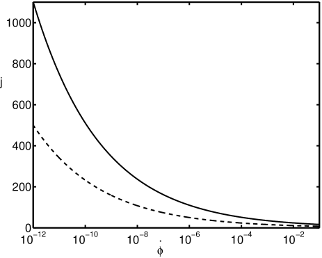
Figure 2: Analytic results for Ham quantization with $l=3/4$ and initial conditions $\phi_{i}=0$ and $\dot{\phi}_{i}>0$. The solid line corresponds to the case where the turning point of the inflaton is at $\phi=3l_{\rm Pl}$. Sufficient inflation to solve the horizon problem arises in the region above this line. The kinetic bound is satisfied in the region below the dashed line. The two regions do not overlap.

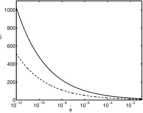
Figure 3: Numerical results corresponding to the scheme shown in Fig. 2.

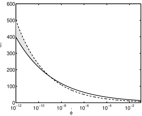
Figure 4: Analytic results for Fried quantization with $l=3/4$ and initial conditions $\phi_{i}=0$ and $\dot{\phi}_{i}>0$. The horizon problem is solved in the region above the solid line and the kinetic bound is satisfied below the dashed line. The shaded area represents the region of parameter space that leads to successful inflation for this set of initial conditions.

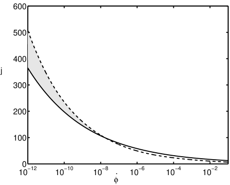
Figure 5: Numerical results corresponding to the scheme shown in Fig 4.

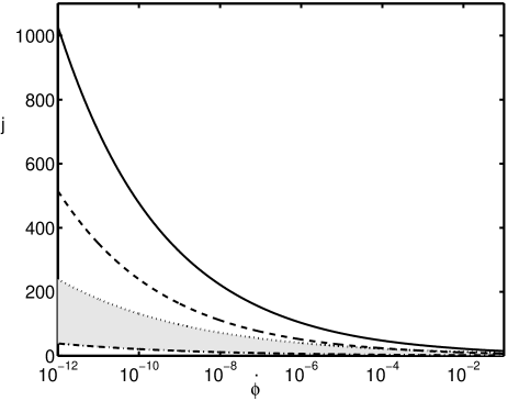
Figure 6: Numerical results for Ham quantization with $l=3/4$, where the initial value of the inflaton is determined by imposing the uncertainty principle (27). The horizon problem is solved in regions above the solid line and below the dotted line. The region below the dashed line satisfies the kinetic bound. The potential energy of the field exceeds the Planck scale below the dot-dashed line. Successful inflation is possible in the shaded region.

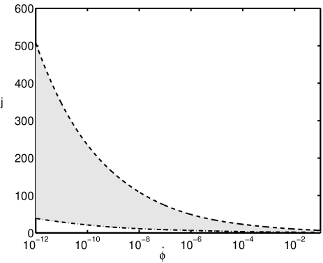
Figure 7: Numerical results for Fried quantization with $l=3/4$, where the initial value of the inflaton is determined by imposing the uncertainty principle (27). The horizon problem is solved for all values of $j$ and $\dot{\phi}_{i}$ covered in the figure. The conditions for successful inflation are therefore limited only by the requirement that the classical phase corresponds to energy scales below the Planck scale. Successful inflation arises in the shaded region.

Figure 8: The behavior of the function $D_{l}$ for different values of $l$.

VI Discussion

In this paper we have considered some of the cosmological consequences of ambiguities that arise in loop quantum gravity. We have focused primarily on the importance of these ambiguities in realizing the conditions that lead to a phase of slow–roll inflation when the inflaton is initially located in a minimum of its potential. We have invoked a semi–classical treatment, where the dynamics of the universe is governed by non–linear ODEs. The key requirement for successful inflation within this framework is that sufficient inflation is possible in the region of parameter space where this approximation remains valid. In particular, this implies that the initial kinetic energy of the inflaton must be sufficiently small.

Our main conclusion is that the initial conditions for slow–roll inflation can be realized in a wide region of parameter space in loop quantum cosmology. In this sense, therefore, LQC is robust to ambiguities in the quantization and enhances the allowed range of initial conditions for inflation. In particular, kinetic energies many orders of magnitude below the Planck scale can lead to inflation. Moreover, parameters can be chosen such that the turning point of the inflaton is near to $3l_{\rm Pl}^{-1}$, corresponding to the largest scales accessible to observations. Equation (48) shows that $\phi_{\max}$ depends only logarithmically on $j$ and $\dot{\phi}_{i}$ and thus is sensitive only to the order of magnitude of those values. (Indeed, by using the Lambert function $W(x)$ defined such that $W(x)e^{W(x)}=x$ and behaving like a logarithm for $x>1$, we have $l_{\rm Pl}\phi_{\rm max}=W(140\sqrt{12\pi}j^{6}|\dot{\phi}_{i}l_{\rm Pl}^{2}|e^{\sqrt{12\pi}l_{\rm Pl}\phi_{i}})$.) This verifies what can already be observed from Fig. 2 of Ref. tsm03 .

For the choice $l=3/4$, conditions for successful inflation can be achieved in the Fried quantization scheme if $j$ is sufficiently high even when the field is located at the potential minimum. The field tends to move further up the potential in the Fried quantization than in Ham quantization. In this sense, Fried quantization might be favored from a phenomenological point of view at the semi–classical level, as it results in a larger region of parameter space for successful inflation (this has already been indicated in golam ). This is interesting given that the Ham quantization scheme is directly based on a Hamiltonian whereas Fried involves additional multiplication with eigenvalues of the geometrical density operator and thus appears less natural conceptually.

In Ham quantization, the field needs to be displaced from its minimum, for example by quantum uncertainty effects, if it is to move sufficiently far up the potential without violating the bounds imposed by the semi–classical approximation. However, care should be taken in interpreting the kinetic bound (40) – the solution (34) overestimates the value of the field’s kinetic energy at the transition since the form of the eigenvalue function, $D_{l}$, given in Eq. (4) represents its asymptotic form in the limit $a\ll a_{*}$. Moreover, the estimate for $a_{S}$, the scale factor at the transition epoch, given in Eq. (IV.2), is not precise, since there is no exact definition for this parameter. If the kinetic bound (40) were to be relaxed slightly, then it would become marginally consistent with the horizon problem constraint (50). This indicates that if successful inflation could be realized within this semi–classical framework, the conditions would be such that just enough e–folds of accelerated expansion would arise for the horizon problem to be solved. As a result, astrophysically observable scales today would correspond to the turning point in the field’s dynamics.

It should be emphasized that failure to satisfy the kinetic bounds does not necessarily rule out certain parameter choices or quantization schemes, but only limits the allowed range where the approximation to ODEs can be employed. When the Hubble length becomes smaller than the fundamental discreteness scale, $a_{i}$, the effective ODEs describing the cosmic dynamics become invalid and must be replaced by the full quantum equations, which are a difference equation for the wave function in the case of loop quantum cosmology bojowald02a . It is possible that in this framework both the Ham and Fried schemes would become equally viable at a phenomenological level.

Considering values $l<3/4$ does not alter the qualitative behavior of the dynamics. In general, for a given initial kinetic energy, this leads to an increase in the lowest value of $j$ consistent with successful inflation in Fried quantization, since the semi–classical phase must last longer. Conversely, when $l>3/4$, successful inflation is possible for lower initial kinetic energies and lower values of $j$. For Ham quantization, reducing $l$ makes it harder to satisfy the horizon and kinetic bounds simultaneously. The kinetic energy of the field increases less rapidly for $l\rightarrow 0$ and it might therefore be expected that it would be easier to satisfy the kinetic bound. However, in this case the field lacks the kinetic energy needed to reach a sufficiently high value after the semi-classical era. Thus, the phenomenological indications for $l$ are in agreement with the expectations from the full theory which lead to $l\geq 1/2$.

In fact, the results allow us to draw further lessons for the full theory. As discussed in §2.2, Ham is analogous to the full quantization procedure whose dynamics is governed by a constraint, while Fried does not have a full analog. From the phenomenological point of view we can separate the range of parameters for different quantizations into three distinct domains: (i) values which do not lead to sufficient slow-roll inflation; (iia) values which lead to sufficient inflation in such a way that the scalar field reaches a turning point around $3l_{\rm Pl}^{-1}$; and (iib) values leading to sufficient inflation with a turning point much higher than $3l_{\rm Pl}^{-1}$. As we have seen, Fried is phenomenologically more robust to ambiguities and most cases fall into class (iib). On the other hand, Ham is less robust but has most realisations in class (iia) which are more likely to lead to observable effects by putting the maximal inflaton value just at the borderline for sufficient inflation. This may indicate that observations of full loop quantum gravity are indeed within reach.

As for $j$, the lower bounds are larger than unity, as expected, but not unreasonably large. Thus, the scenario appears realistic and does not require fine tuning, which is also a consequence of the weak logarithmic dependence of $\phi_{\rm max}$ on $j$.

A key open question in LQC concerns the evolution of scalar (density) and tensor (gravitational wave) perturbations generated during the semi–classical epoch. Although standard perturbation theory is unstable in this regime tsm03 , it is possible that these perturbations may imprint characteristic signatures of this phase on the CMB power spectrum. Indeed, there have recently been a number of suggestions for explaining the apparent suppression of the CMB power spectrum on large angular scales through quantum gravity effects, including LQC tsm03 , non–commutative geometry roy1 and higher–order curvature terms in string–inspired models shinji . It is important, therefore, to investigate whether observations will be able to discriminate between these different possibilities. Finally, it would also be interesting to extend the analysis of this work to the regime of the quantum difference equations of the full theory and to investigate whether any observable effects for the different quantization schemes can be uncovered.

Acknowledgments

We are grateful to Roy Maartens for discussions. DM is supported by a PPARC studentship. PS thanks Queen Mary, University of London for warm hospitality during the initial stages of this work. He is supported by a CSIR grant.

Appendix A Inverse metric in the full theory

Loop quantum gravity is based on a classical formulation of general relativity using Ashtekar variables. These variable are the densitized triad $E^{a}_{i}$, related to the spatial metric via

$$E^{a}_{i}E^{b}_{i}=q^{ab}\det q$$

and the connection $A_{a}^{i}=\Gamma_{a}^{i}-\gamma K_{a}^{i}$ forming a conjugate pair. Here, $\Gamma_{a}^{i}$ is the spin connection of the triad, $K_{a}^{i}$ the extrinsic curvature, and $\gamma$ the Barbero–Immirzi parameter.

The quantization then proceeds by using as basic quantities holonomies of the connection, $h_{e}(A)={\cal P}\exp\int_{e}A$ for curves $e$ in space, and fluxes computed from the triad, $F_{S}(E)=\int_{S}E$ for spatial surfaces $S$. The important feature of these expressions is that they are defined in a background independent way, i.e., we do not need to choose a metric to define the integration. Yet, by integrating the basic fields $E^{a}_{i}$, $A_{a}^{i}$ are smeared which renders the quantization well-defined.

The background independence in particular requires the density weight employed in the triad $E^{a}_{i}$. This means that the un-densitized triad $e^{a}_{i}=E^{a}_{i}/\sqrt{|\det E|}$ and also the co-triad $e_{a}^{i}=(e^{-1})_{a}^{i}$ are obtained by dividing by $\sqrt{|\det E|}$ and inverting. In general this is ill-defined given that there may be possibly degenerate triads. Nevertheless, it is possible to compute the co-triad, say, from the basic quantities in a well-defined way since qsdi

$$e_{a}^{i}(x)=\frac{1}{4\pi G\gamma}\{A_{a}^{i}(x),\int d^{3}y\sqrt{|\det E(y)|}\}$$ (63)

where we have employed the Poisson bracket and integrated over an arbitrary region containing $x$. This expression does not involve inverses and can be quantized in a well-defined way using holonomies, the volume operator, and turning the Poisson bracket into a commutator. Such classical identities lie at the heart of quantizing expressions as matter Hamiltonians in the full theory thiemann_matter and the geometrical density in isotropic models.

For a scalar field Hamiltonian we need a quantization of $|\det E|^{-1/2}$, which reduces to $a^{-3}$ in an isotropic model. The identity (63) cannot be used immediately, but we can make another reformulation:

$$\frac{1}{\sqrt{|\det E|}}=\frac{\det e}{\det E}=\frac{\frac{1}{6}\epsilon^{abc}\epsilon_{ijk}e_{a}^{i}e_{b}^{j}e_{c}^{k}}{\det E}$$

$$=\frac{1}{6}\epsilon^{abc}\epsilon_{ijk}(4\pi G\gamma)^{3}\{A_{a}^{i},V^{1/3}\}\{A_{b}^{j},V^{1/3}\}\{A_{c}^{j},V^{1/3}\}$$

by writing $V$ for $\int d^{3}y\sqrt{|\det E(y)|}$. This expression can now be embedded in the full matter Hamiltonian and quantized in a background independent way (see thiemann_matter for details). Upon inserting isotropic variables and expressing the connection via holonomies, one can easily check that one obtains (23) with $l=1/2$ (in the Poisson brackets we have simply $a=V^{1/3}$ in both cases).

Even taking into account the need for a background independent quantization, there is still some freedom in the full theory. For example, we can multiply by any positive integer power of $\det e$, such that

$$\frac{1}{\sqrt{|\det E|}}=\frac{(\det e)^{k}}{(\det E)^{(k+1)/2}}=\left(\frac{1}{6}\epsilon^{abc}\epsilon_{ijk}(4\pi G\gamma)^{3}\right.$$

$$\times\{A_{a}^{i},V^{(2k-1)/3k}\}\{A_{b}^{j},V^{(2k-1)/3k}\}\{A_{c}^{j},V^{(2k-1)/3k}\}\Bigr{)}^{k}$$

with a discrete rather than a continuous set of the ambiguity parameter. When evaluating in isotropic variables, we obtain the form (23) with $l_{k}=1-(2k)^{-1}\geq 1/2$. The value $l_{2}=3/4$ results from using $\det E$ to multiply and this seems the most natural choice when we keep in mind that $E$, rather than $e$, is the basic geometrical variable underlying loop quantum gravity. The analogous reformulation of $1/\sqrt{|\det E|}$ has been used in thiemann_matter for a full scalar Hamiltonian (see §3.3 of that work). Moreover, since $l_{2}$ is the midpoint of the set spanned by the values $l_{k}$, it should give representative results.

References

- (1) C. Rovelli, Liv. Rev. Rel. 1, 1 (1998) [arXiv:gr-qc/9710008].
- (2) T. Thiemann, Lect. Notes Phys. 631, 41 (2003) [arXiv:gr-qc/0210094].
- (3) C. Rovelli & L. Smolin, Nucl. Phys. B 442, 593 (1995) [arXiv:gr-qc/9411005]; A. Ashtekar & J. Lewandowski, Class. Quant. Grav. 14, A55 (1997) [arXiv:gr-qc/9602046]; T. Thiemann, J. Math. Phys. 39, 3347 (1998) [arXiv:gr-qc/9606091].
- (4) T. Thiemann, Class. Quant. Grav. 15, 1281 (1998) [arXiv:gr-qc/9705019].
- (5) K. Krasnov, Gen. Rel. Grav. 30, 53 (1998) [arXiv:gr-qc/9605047]; C. Rovelli, Phys. Rev. Lett. 77, 3288 (1996) [arXix:gr-qc/9603063]; A. Ashtekar, J. Baez, A. Corichi & K. Krasnov, Phys. Rev. Lett. 80, 904 (1998) [arXiv:gr-qc/9710007].
- (6) M. Bojowald & H. A. Morales-Técotl, Lect. Notes Phys. (in press) [arXiv:gr-qc/0306008].
- (7) M. Bojowald & K. Vandersloot, arXiv:gr-qc/0312103.
- (8) M. Bojowald, Pramana (in press) [arXiv:gr-qc/0402053].
- (9) M. Bojowald, Phys. Rev. Lett. 86, 5227 (2001) [arXiv:gr-qc/0102069].
- (10) M. Bojowald, Phys. Rev. Lett. 87, 121301 (2001) [arXiv:gr-qc/0104072].
- (11) M. Bojowald & G. Date, Phys. Rev. Lett. 92, 071302 (2004) [arXiv:gr-qc/0311003].
- (12) M. Bojowald, Phys. Rev. Lett. 89, 261301 (2002) [arXiv:gr-qc/0206054].
- (13) M. Bojowald & K. Vandersloot, Phys. Rev. D 67, 124023 (2003) [arXiv:gr-qc/0303072].
- (14) S. Tsujikawa, P. Singh & R. Maartens, arXiv:astro-ph/0311015.
- (15) P. Singh & A. Toporensky, Phys. Rev. D (in press) [arXiv:gr-qc/0312110].
- (16) M. Bojowald, Class. Quant. Grav. 19, 5113 (2002) [arXiv:gr-qc/0206053].
- (17) M. Bojowald, Class. Quant. Grav. 19, 2717 (2002) [arXiv:gr-qc/0202077].
- (18) G. M. Hossain, Class. Quant. Grav. 21, 179 (2003).
- (19) M. Bojowald, Phys. Rev. D 64, 084018 (2001) [arXiv:gr-qc/0105067].
- (20) A. Ashtekar, M. Bojowald & J. Lewandowski, Adv. Theor. Math. Phys. 7, 233 (2003) [arXiv:gr-qc/0304074].
- (21) A. D. Linde, Phys. Lett. 129B, 177 (1983).
- (22) A. R. Liddle and D. H. Lyth, Cosmological Inflation and Large-Scale Structure (Cambridge University Press, Cambridge, 2000).
- (23) D. N. Spergel et al., Astrophys. J. Suppl. 148, 175 (2003) [arXiv:astro-ph/0302209]; H. V. Peiris et al., Astrophys. J. Suppl. 148, 213 (2003) [arXiv:astro-ph/0302225].
- (24) M. S. Madsen and P. Coles, Nucl. Phys. B 298, 701 (1988).
- (25) S. Tsujikawa, R. Maartens & R. Brandenberger, Phys. Lett. B 574, 141 (2003) [arXiv:astro-ph/0308169].
- (26) Y-S Piao, S. Tsujikawa & X. Zhang, arXiv:hep-th/0312139.
- (27) T. Thiemann, Class. Quant. Grav. 15, 839 (1998) [arXiv:gr-qc/9606089].