Testing Alternative Theories of Gravity using LISA

Abstract

We investigate the possible bounds which could be placed on alternative theories of gravity using gravitational wave detection from inspiralling compact binaries with the proposed LISA space interferometer. Specifically, we estimate lower bounds on the coupling parameter $\omega$ of scalar-tensor theories of the Brans-Dicke type and on the Compton wavelength of the graviton $\lambda_{g}$ in hypothetical massive graviton theories. In these theories, modifications of the gravitational radiation damping formulae or of the propagation of the waves translate into a change in the phase evolution of the observed gravitational waveform. We obtain the bounds through the technique of matched filtering, employing the LISA Sensitivity Curve Generator (SCG), available online. For a neutron star inspiralling into a $10^{3}\,M_{\odot}$ black hole in the Virgo Cluster, in a two-year integration, we find a lower bound $\omega>3\times 10^{5}$. For lower-mass black holes, the bound could be as large as $2\times 10^{6}$. The bound is independent of LISA arm length, but is inversely proportional to the LISA position noise error. Lower bounds on the graviton Compton wavelength ranging from $10^{15}$ km to $5\times 10^{16}$ km can be obtained from one-year observations of massive binary black hole inspirals at cosmological distances (3 Gpc), for masses ranging from $10^{4}$ to $10^{7}\,M_{\odot}$. For the highest-mass systems ($10^{7}\,M_{\odot}$), the bound is proportional to (LISA arm length)^1/2 and to (LISA acceleration noise)^-1/2. For the others, the bound is independent of these parameters because of the dominance of white-dwarf confusion noise in the relevant part of the frequency spectrum. These bounds improve and extend earlier work which used analytic formulae for the noise curves.

1 Introduction and summary

The Laser Interferometer Space Antenna (LISA) is a gravitational-wave detector being designed for launch in the 2010-2015 time frame [1]. Consisting of a triangular array of three satellites orbiting the Sun on an Earth-like orbit, it will use laser interferometry to open up the low-frequency gravitational-wave window, to complement the high-frequency window currently being explored by ground-based interferometers. It is expected to be able to observe waves from known binary star systems, from a background of white-dwarf binaries, from inspirals of black holes and other compact bodies into massive black holes, and possibly from phase transitions in the early universe.

LISA may also provide new and interesting tests of fundamental physics. In previous papers [2, 3, 4], we showed how observations of waves from inspiralling compact binaries could place bounds on alternative theories of gravity, such as theories of the scalar-tensor type (e.g. Brans-Dicke theory), or theories with a massive graviton.

In scalar-tensor theories, the phenomenon of dipole gravitational radiation modifies the damping of the binary orbit, and thereby alters the evolution of the phasing of the received wave, compared to what general relativity would predict. We showed, for example, that, for the inspiral of a neutron star into a black hole of mass $10^{3}\,{\rm M}_{\odot}$ at a distance of 50 Mpc, the lower bound on the coupling parameter $\omega$ would be $2.4\times 10^{5}$, with one year of integration prior to the innermost stable orbit [4]. The bound falls off with increasing mass.

In massive graviton theories, the wavelength-dependent propagation speed of the waves and the resulting arrival-time offsets also modify the evolution of phasing of the received wave, compared to general relativity. For the inspiral of two $10^{6}\,M_{\odot}$ black holes at 3 Gpc, we showed that the lower bound on the graviton Compton wavelength $\lambda_{g}$ would be $5.4\times 10^{16}$ km, over four orders of magnitude larger than the bound inferred from solar-system dynamics.

Several developments have motivated us to revisit these bounds. One is the dramatic improvement in the solar-system bound on scalar-tensor gravity via tracking of the Cassini spacecraft [5]. The new bound is $\omega>4\times 10^{4}$. Another is the increasing interest in massive gravity theories, from the viewpoint both of conventional modifications of general relativity [6, 7], and of multidimensional or brane-world theories [8].

The third factor is the availability of an improved noise curve for the LISA detector. Earlier work employed an analytic approximation to LISA’s instrumental noise based on the LISA Phase A study [9, 10], augmented by an estimate of white-dwarf confusion noise in the low-frequency regime [11]. The improved curves, based on work by Larson et al. and Armstrong et al. [12, 13], additionally take into account the finite propagation time of the laser signals during the passage of the gravitational wave, which is embodied in a transfer function that modifies the response of LISA at high frequencies. In addition, the curves are available online in a “Sensitivity Curve Generator” (SCG) [14], that permits the user to modify the parameters of LISA (arm length, position noise budget, etc) so as to explore the capabilities of different hypothetical LISA instruments. The main difference between the analytic curves used earlier and those from the SCG, apart from the characteristic oscillations at high frequency arising from the transfer function, is that the amplitude noise level of the latter is roughly a factor of 3 higher (see figure 1). This will have an effect on some of the bounds we report.

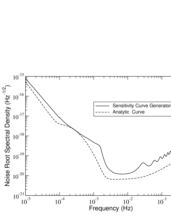
Figure 1: LISA root spectral noise density vs. frequency, including white-dwarf confusion noise. Shown is the nominal LISA curve from the Sensitivity Curve Generator, and the analytic curve used in [3, 4]

We use the method of parameter estimation via matched filtering to estimate bounds on alternative theories. The idea of matched filtering is to cross-correlate a theoretical template gravitational waveform against the output of the detector. The template may depend on a number of parameters, such as the masses of the stars, and parameters associated with the theory of gravity. One can then calculate, for a given set of parameters and for a given spectrum of noise in the detector, how accurately the parameters inherent in the true signal can be estimated [15, 16, 17, 18, 19].

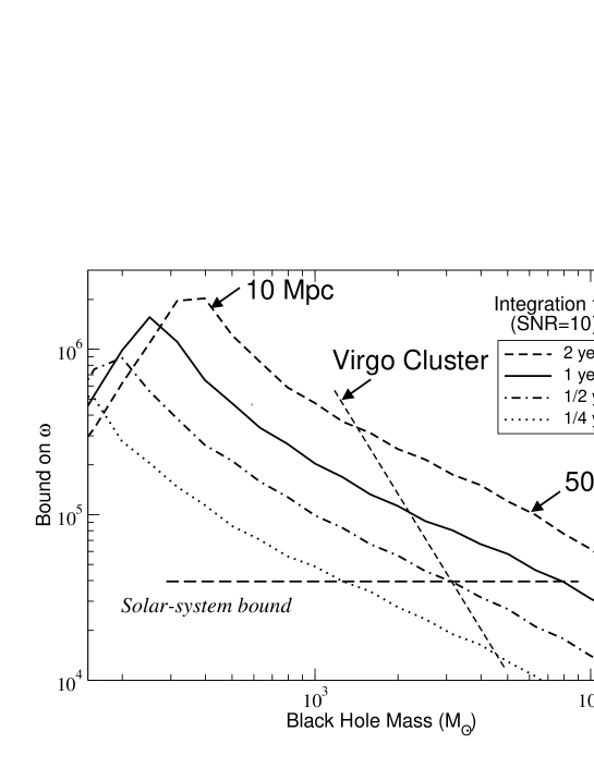
Figure 2: Bound on Brans-Dicke $\omega$ vs. black-hole mass, assuming SNR$=10$

For testing scalar-tensor theories, the best system is binary inspiral of a neutron star into a black hole. We consider quasi-circular inspiral of non-spinning bodies ending at the innermost stable circular orbit (ISCO). Assuming detection with a signal-to-noise ratio (SNR) of 10, we find lower bounds on $\omega$ shown in figure 2, for various integration times. Also shown are representative distances of the sources observed, along with the solar-system bound from Cassini. The sharp decrease in the bounds for BH masses below a few hundred solar masses results from the fact that the signal falls off the high-frequency end of the LISA sensitivity curve before the system reaches the ISCO. The bounds shown in figure 2 are only slightly changed from our earlier bounds (figure 1 of [4]). For a fixed SNR, the bounds depend on the shape of the noise curve, not on its overall scale (the oscillations from the transfer function tend partially to average out). The change occurs in the distance at which a given source can be detected, or in the bound obtained from a source at a given distance. Both have decreased by about a factor of three, consistent with the shift observed in figure 1. We also find that, for a source at a given distance, the bound is relatively insensitive to LISA arm length but is inversely proportional to LISA position error.

For testing massive graviton theories, the best systems are massive black hole binaries. Again we consider quasi-circular inspiral of non-spinning bodies ending at the innermost circular orbit. For sources at a redshift $Z=1/2$, we find lower bounds on $\lambda_{g}$ shown in figure 3. The bounds are plotted for various total masses as a function of the reduced mass parameter $\eta=m_{1}m_{2}/(m_{1}+m_{2})^{2}$, which varies from zero to $1/4$. The curves terminate at the small mass ratio end where the SNR drops below 10. For sources at a given distance, the bounds on $\lambda_{g}$ are weaker than those reported earlier [3] by a factor of about $\sqrt{3}$ (square root because of the quadratic dependence of the effect on $\lambda_{g}$), again reflecting the higher noise level generated by the SCG compared to our earlier formula. For the highest mass systems, e.g. $10^{7}\times 10^{7}M_{\odot}$, the bound is proportional to (LISA arm length)^1/2 and to (LISA acceleration noise)^-1/2. This dependence becomes progressively weaker with decreasing mass, so that for $10^{4}\times 10^{4}M_{\odot}$ systems, the bound is independent of these parameters. This is because the signals from high mass systems reside at the low frequency end of the LISA noise curve, where arm length or acceleration noise affect the noise in the expected fashion, whereas the signals from lower mass systems reside in the regime where the noise is dominated by white-dwarf confusion noise.

The bounds shown in figure 3 should be compared to bounds inferred from the validity of static Newtonian gravity over large distances, of $2.8\times 10^{12}$ km from solar-system dynamics [20], and $6\times 10^{19}$ km from cluster dynamics [21].

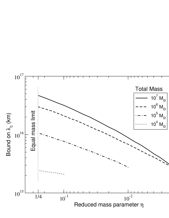
Figure 3: Bound on graviton Compton wavelength $\lambda_{g}$ vs. $\eta=m_{1}m_{2}/(m_{1}+m_{2})^{2}$, for massive black hole binaries at $Z=1/2$.

The remainder of this paper provides details. In section 2 we review the method of parameter estimation using matched filtering within general relativity. Section 3 treats scalar-tensor bounds and massive graviton bounds. Section 4 presents concluding remarks.

2 Parameter estimation using matched filtering

2.1 Estimation in general relativity

In this section we review briefly the technique used for estimating parameters of inspiralling binaries using matched filtering, in the context of general relativity. Further details may be found in [16, 17, 18, 19]. In matched filtering, a template consisting of a theoretical gravitational waveform is compared to the detector output. The template that is a match with an actual signal present with the noise will show a strong correlation with the detector output and thereby will “filter” a signal out of background noise. The template is represented by $h(t)$, related to the spatial components of the radiative metric perturbation far from the source. We adopt the so-called “restricted post-Newtonian approximation” for an inspiral orbit that is quasi-circular (that is, circular apart from the adiabatic decrease in separation), wherein we approximate $h(t)\approx h_{0}(t)e^{i\Phi(t)}$, where $h_{0}(t)$ is a slowly varying wave amplitude which depends on the wave polarization, the location of the source on the sky, the detector orientation, and the distance to the source. The wave phase, $\Phi(t)$, is a function of the evolving orbital frequency. Because the process of matched-filtering is sensitive mostly to the phasing of the wave, the amplitude $h_{0}(t)$ is assumed to be given by the lowest-order, quadrupole approximation, while $\Phi(t)$ is taken to a suitably high post-Newtonian order. The Fourier transform of $h(t)$ using the stationary phase approximation is given by

$$\tilde{h}(f)=\left\{\begin{array}[]{ll}{\cal A}f^{-7/6}e^{i\Psi(f)}\,,&0<f<f_{\rm max}\,,\\ 0\,,&f>f_{\rm max}\,,\end{array}\right.$$ (1)

where $f_{\rm max}$ is the largest frequency for which the wave can be described by the restricted post-Newtonian approximation, often taken to correspond to waves emitted at the innermost stable orbit (ISCO) before the bodies plunge toward each other and merge. A useful approximation for this frequency is (we use units in which $G=c=1$)

$$f_{\rm max}=(6^{3/2}\pi m)^{-1},$$ (2)

where $m$ is the total mass of the system. After averaging over all angles, the amplitude $\cal A$ is given by

$${\cal A}=\frac{1}{\sqrt{30}\pi^{2/3}}\frac{{\cal M}^{5/6}}{D_{L}}\,,$$ (3)

where $D_{L}$ is the luminosity distance of the source, and ${\cal M}=\eta^{3/5}m$ is the “chirp” mass. In general relativity, the phasing function $\Psi(f)$ is given, through 1.5 post-Newtonian (PN) order, for spinless bodies, by

$$\Psi(f) = 2\pi ft_{c}-\phi_{c}-\frac{\pi}{4}$$ (4)

$$+\frac{3}{128}u^{-5/3}\left[1+\frac{20}{9}\left(\frac{743}{336}+\frac{11}{4}\eta\right)\eta^{-2/5}u^{2/3}-16\pi\eta^{-3/5}u\right]\,,$$

where $u=\pi{\cal M}f$ ($u\sim v^{3}$) and $\phi_{c}$ is formally defined as the phase of the wave at the time of coalescence, $t_{c}$. (Terms through 3.5PN order are known [22] but will not be used here.)

By maximizing the correlation between a template waveform that depends on a set of parameters $\theta^{a}$ (for example, the chirp mass $\cal M$) and a measured signal, matched filtering provides a natural way to estimate the parameters of the signal and their errors. With a given detector noise spectral density $S_{n}(f)$ one defines the inner product between two signals $h_{1}(t)$ and $h_{2}(t)$ by

$$(h_{1}|h_{2})\equiv 2\int_{0}^{\infty}\frac{{\tilde{h}_{1}}^{*}\tilde{h}_{2}+{\tilde{h}_{2}}^{*}\tilde{h}_{1}}{S_{n}(f)}df\,,$$ (5)

where $\tilde{h}_{1}(f)$ and $\tilde{h}_{2}(f)$ are the Fourier transforms of the respective gravitational waveforms $h(t)$. The signal-to-noise ratio (SNR) for a given $h$ is given by

$$\rho[h]\equiv(h|h)^{1/2}\,.$$ (6)

One then defines the “Fisher information matrix” $\Gamma_{ab}$ with components given by

$$\Gamma_{ab}\equiv\left(\frac{\partial h}{\partial\theta^{a}}\mid\frac{\partial h}{\partial\theta^{b}}\right)\,,$$ (7)

An estimate of the rms error, $\Delta\theta^{a}$, in measuring the parameter $\theta^{a}$ can then be calculated, in the limit of large SNR, by taking the square root of the diagonal elements of the inverse of the Fisher matrix,

$$\Delta\theta^{a}=\sqrt{\Sigma^{aa}}\,,\qquad\Sigma=\Gamma^{-1}\,.$$ (8)

The correlation coefficients between two parameters $\theta^{a}$ and $\theta^{b}$ are given by

$$c_{ab}=\Sigma^{ab}/\sqrt{\Sigma^{aa}\Sigma^{bb}}\,.$$ (9)

In general relativity, the parameters to be estimated using the above template would be $\phi_{c}$, $f_{0}t_{c}$, $\ln{\cal M}$, and $\ln\eta$, where $f_{0}$ is a fiducial frequency characteristic of the detector noise spectrum. The method then follows that used, for example, in [19]: combining equations (1) and (4) and calculating the partial derivatives $\partial{\tilde{h}}/\partial\theta^{a}$ for the four listed parameters, we construct the Fisher information matrix using equations (5) and (7). We then invert the information matrix and evaluate the errors in the four parameters, along with the correlation coefficients, notably between $\cal M$ and $\eta$. For the alternative Brans-Dicke or massive graviton theories to be considered here, we will add a suitable term to the phasing $\Psi(f)$, dependent upon an additional parameter $\theta$. We will augment the dimension of the Fisher matrix by one, and estimate five parameters, along with the correlation coefficients between $\cal M$, $\eta$ and $\theta$. Since the nominal value of $\theta$ will be assumed to be zero (corresponding to $\omega=\infty$ or $\lambda_{g}=\infty$), the error on $\theta$ will translate into a lower bound on $\omega$ or $\lambda_{g}$.

2.2 Space-based interferometers

We consider space-based interferometers of the proposed LISA type, with a sensitive bandwidth between $10^{-5}$ and $1$ Hz, and an expected noise curve which can be expressed in terms of an overall amplitude $S_{0}$, and a function of the ratio $x=f/f_{0}$:

$$S_{n}(f)=S_{0}g(x)\,.$$ (10)

In earlier work [3, 4] we adopted an analytic noise curve that included the LISA instrumental noise and an estimate of “confusion noise” from a population of galactic white-dwarf binaries [9, 10, 11] given by

$$S_{0} = 4.2\times 10^{-41}\,{\rm Hz}^{-1}\,,$$

$$f_{0} = 10^{-3}{\rm Hz}\,,$$

$$g(x) = \sqrt{10}x^{-14/3}+1+x^{2}/1000+313.5x^{-(6.398+3.518\log_{10}x)}\,.$$ (11)

In this paper, we will retain the scaling using $S_{0}$ and $f_{0}$, which is useful for expressing analytic results, but for $g(x)$ we will use values obtained from data files available on line using the LISA “Sensitivity Curve Generator” (see section 2.3).

In terms of this scaling, the SNR is given, from equations (1), (5) and (6), by

$$\rho^{2}=4|{\cal A}|^{2}f_{0}^{-4/3}I(7)/S_{0},$$ (12)

where we define the integrals $I(q)$ by

$$I(q)=\int_{x_{\rm min}}^{x_{\rm max}}\frac{x^{-q/3}}{g(x)}dx\,,$$ (13)

where $x_{\rm min}=f_{\rm min}/f_{0}$ and $x_{\rm max}=f_{\rm max}/f_{0}$, corresponding to the minimum and maximum frequencies over which the detector will integrate . In some calculations, the maximum value of $f_{\rm max}$ corresponds to radiation emitted at the ISCO of the system, while in others, we can consider the effect of terminating observations sooner than this final orbit. The frequency $f_{\rm min}$ corresponds to the gravitational-wave frequency observed a time $T$ earlier, where for LISA-type systems, we will assume $T\leq$ two years. Using the quadrupole approximation for radiation damping, which is an adequate approximation for this purpose, one can relate the frequencies of gravitational radiation at the beginning and end of any time interval $T$ by the expression

$$u_{i}=u_{f}\left(1+{256\over 5}{T\over{\cal M}}u_{f}^{8/3}\right)^{-3/8}\,.$$ (14)

The luminosity distance $D_{L}$ to which such sources can be detected can be obtained from equations (3) and (12), and related to source masses, detector characteristics and the SNR:

$$D_{L}=\sqrt{\frac{2}{15}}\frac{{\cal M}^{5/6}}{\rho}(\pi f_{0})^{-2/3}\left(\frac{I(7)}{S_{0}}\right)^{1/2}$$

$$\qquad=2.45\,{\rm Gpc}\left(\frac{m_{NS}}{1.4M_{\odot}}\right)^{1/2}\left(\frac{m_{BH}}{10^{4}M_{\odot}}\right)^{1/3}\left(\frac{10}{\rho}\right)\left(\frac{4.2\times 10^{-41}}{S_{0}}\right)^{1/2}\left(\frac{10^{-3}}{f_{0}}\right)^{2/3}I(7)^{1/2}$$

$$\qquad=4.81\,{\rm Gpc}(4\eta)^{1/2}\left(\frac{m_{Tot}}{10^{6}M_{\odot}}\right)^{5/6}\left(\frac{10^{4}}{\rho}\right)\left(\frac{4.2\times 10^{-41}}{S_{0}}\right)^{1/2}\left(\frac{10^{-3}}{f_{0}}\right)^{2/3}I(7)^{1/2}\,.$$ (15)

2.3 Sensitivity curves for LISA

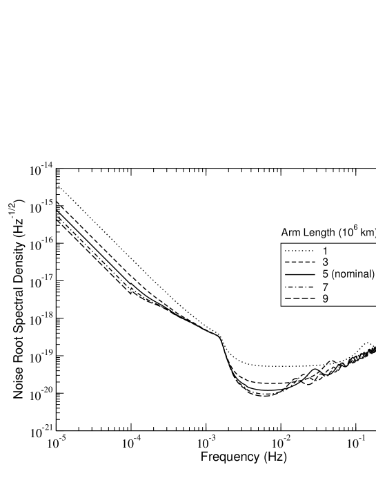
Figure 4: LISA noise root spectral density for varying arm length

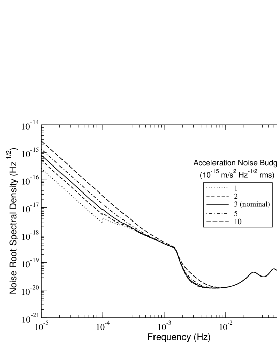
Figure 5: LISA noise root spectral density for varying acceleration noise

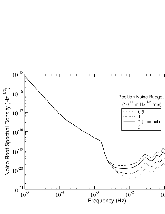
Figure 6: LISA noise root spectral density for varying position noise

In this paper, we shall adopt sensitivity curves for LISA developed independently by Larson et al. [12] and Armstrong et al. [13]. The two methods are in substantial agreement, and the former has been summarized in the Sensitivity Curve Generator (SCG), available online [14]. The sensitivity curves incorporate sources of instrumental noise in LISA, such as laser shot noise, acceleration noise, thermal noise, etc., coupled with a LISA transfer function which takes into account the effect of the finite time of propagation of the laser beams during the passage of the gravitational waves. We assume the case where all three arms of LISA are of equal length, and we assume that averages over angles and polarizations have been done. The SCG permits various choices to be made for LISA instrumental parameters, and has an option to include an estimate for confusion noise resulting from a background of galactic white-dwarf binaries [11]; this background is included in our analyses.

For the baseline LISA proposal, the noise root spectral density ($h$ per $\sqrt{Hz}$) is shown in figure 1, along with the analytic curve used in earlier work. The oscillations at the high-frequency end result from the transfer function. Notice that the SCG amplitude noise level is about a factor of 3 larger than the analytic curve. This has the effect of weakening our bounds on $\omega$ and $\lambda_{g}$ relative to earlier work.

In order to study the effect of varying LISA parameters on our tests of alternative theories, we vary the arm length, the acceleration noise budget and the position noise budget. The resulting curves (including the WD confusion noise) are shown in figures 4 – 6. Varying arm length and acceleration noise affects primarily the low-frequency noise, while varying the position noise budget affects primarily the high-frequency end. Varying other parameters in the SCG, such as laser power or wavelength, or telescope diameter, has no sizable effect on the noise curve or on the bounds.

3 Testing alternative theories of gravity

3.1 Bounding scalar-tensor theories of the Brans-Dicke type

One of the most striking differences between scalar-tensor theories and general relativity is the prediction of dipole gravitational radiation. The source of such radiation is the difference between the self-gravitational binding energy per unit mass between the two bodies in a binary system, as encoded in a “sensitivity” $s$ (technically, the sensitivity of the body’s total mass to variations in the locally measured value of the gravitational constant). For black holes, $s\equiv 0.5$, while for neutron stars, $s\sim 0.1-0.2$, depending on the equation of state. In principle, dipole radiation can be a strong effect, because it depends on two powers of velocity fewer than quadrupole radiation. This additional source of energy flux will alter the inspiral orbit of the binary, and thus will modify the evolution of the waveform phasing.

To sufficient accuracy, this can be taken into account in our phasing function $\Psi(f)$ by adding the following term to the general relativistic formula, equation (4):

$$\delta\Psi(f)=\frac{3}{128}u^{-5/3}\left(-\frac{5}{84}\frac{{\cal S}^{2}}{\omega}\eta^{2/5}u^{-2/3}\right)\,,$$ (16)

where ${\cal S}=s_{1}-s_{2}$ (see [2, 4] for details). In doing so, we are assuming that $\omega\gg 1$, to be consistent with the solar-system bound $\omega>40,000$, so that the $O(1/\omega)$ corrections to the general relativistic terms in equation (4) may be ignored compared to the dipole term of equation (16). Notice that, compared to the leading term “1” in equation (4), the dipole term is $O(u^{-2/3})\sim O(1/v^{2})$.

Because $s=0.5$ for black holes, binary black holes do not emit dipole radiation at all. For neutron stars, $s$ is a relatively weak function of mass, and so for binary neutron stars with masses near $1.4\,M_{\odot}$, dipole radiation is suppressed by symmetry. The only promising sources, then, are mixed, such as black-hole neutron-star systems (black-hole white-dwarf systems were discussed in [4]).

$m_{BH}$	$\Delta t_{c}$	$\Delta\Phi_{c}$	$\Delta{\cal M}/{\cal M}$	$\Delta\eta/\eta$	Bound	$c_{\eta{\cal M}}$	$c_{{\cal M}\tilde{b}}$	$c_{\eta\tilde{b}}$
$(M_{\odot})$	(s)		(%)	(%)	on $\omega$
1000	3.94	18.3	.000222	.1034	203772	.886	-.994	-.929
5000	3.78	11.5	.000528	.0246	58020	.970	-.998	-.954
10000	5.27	12.6	.000739	.0174	31062	.976	-.997	-.957

Table 1: Estimated parameter errors for $1.4\,M_{\odot}$ NS-MBH systems in Brans-Dicke theory: SNR = 10, integration time is one year prior to the ISCO, neutron star sensitivity $s_{NS}=0.2$.

We now carry out the parameter estimation calculation for the parameters $\phi_{c}$, $f_{0}t_{c}$, $\ln{\cal M}$, $\ln\eta$, and $b\equiv 5{\cal S}^{2}\eta^{2/5}/48\omega$ ($b\to 0$ in the GR limit). We consider a neutron star of mass $1.4\,M_{\odot}$ in a quasicircular inspiral orbit around a black hole of mass $m_{BH}$. We adopt the value $s_{NS}=0.2$. The results of the parameter estimation for various black-hole masses are shown in table 1, and the bounds on $\omega$ as a function of black hole mass and for various integration times are shown in figure 2. For black holes less massive than a few thousand solar masses, the bounds could exceed the current solar system bound. figure 7 shows, for a $10^{3}\,M_{\odot}$ black hole, the bound that could be achieved for sources at various redshifts, and as a function of the LISA position error budget ($2\times 10^{-11}\,{\rm m}/\sqrt{\rm Hz}$ is the nominal value). Since $\Delta b\propto 1/\rho$, the bound on $\omega$ should be inversely proportional to the position error budget, as confirmed in figure 7. The bounds can also be shown to be relatively insensitive to LISA arm length or acceleration noise. These results are consistent with figures 4 – 6, since the relevant sources are concentrated at the high-frequency end of the LISA noise spectrum, where the noise spectral density is affected by position errors but not by arm length or acceleration noise. These bounds for sources at a set distance, are roughly a factor 3 weaker than the bounds estimated in [4], as expected from the overall shift shown in figure 1.

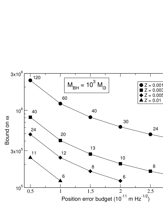
Figure 7: Bound on $\omega$ vs. LISA position error, for sources at various redshifts. Shown are values of the SNR for representative points.

3.2 Bounding massive graviton theories

Notwithstanding statements in the literature forbidding theories of gravity with a massive graviton [23, 24], such theories have attracted considerable recent interest, from the point of view of conventional modifications of classical GR [25, 6, 7], and from considerations of extra dimensions [8]. To the extent that a candidate massive graviton theory merges smoothly with GR in the limit that the graviton mass $m_{g}$ vanishes or its Compton wavelength $\lambda_{g}\to\infty$, one might reasonably expect corrections to GR results for the intrinsic behaviour of a system to be of order $(R/\lambda_{g})^{2}$, where $R$ is the characteristic size of the system. Since solar system measurements already constrain $\lambda_{g}>10^{12}$ km, such corrections can be ignored for inspiralling compact binaries. The dominant effect of a massive graviton is via the propagation of the waves: lower frequency waves propagate more slowly than higher frequency waves. For binary inspiral seen at cosmological distances, this wavelength dependent speed difference can result in a significant cumulative distortion of the apparent phasing of the observed chirp gravitational-wave signal. The effect is to add the following term to the general relativistic formula, equation (4):

$$\delta\Psi(f)=\frac{3}{128}u^{-5/3}\left(-\frac{128}{3}\frac{{\pi^{2}D\cal M}}{\lambda_{g}^{2}(1+Z)}u^{2/3}\right)\,,$$ (17)

where $Z$ is the redshift of the source, and $D=(1+Z)\int_{t_{e}}^{t_{0}}[a(t)/a(t_{0})]dt$, where $a(t)$ is the cosmological scale factor, and $t_{e}$ and $t_{0}$ are the times of emission and reception of the gravitational-wave (see [3] for details). The “distance” $D$ arises from the wavelength-dependent propagation of the gravitational wave signal. It is related to the normal luminosity distance $D_{L}$ by $D/D_{L}=[1+(2+Z)(1+Z+\sqrt{1+Z})]/5(1+Z)^{2}$ in a spatially flat, matter dominated universe.

$m_{1}$	$m_{2}$	SNR	$\Delta t_{c}$	$\Delta\Phi_{c}$	$\Delta{\cal M}/{\cal M}$	$\Delta\eta/\eta$	Bound on	$c_{\eta{\cal M}}$	$c_{{\cal M}\beta}$	$c_{\eta\beta}$
$(M_{\odot})$	$(M_{\odot})$		(s)		(%)	(%)	$\lambda_{g}$ (km)
$10^{7}$	$10^{7}$	1023	31.3	.119	.0316	.945	$4.8\times 10^{16}$	-.979	-.991	.997
$10^{6}$	$10^{6}$	984	1.65	.048	.0050	.276	$3.1\times 10^{16}$	-.965	-.988	.993
$10^{5}$	$10^{5}$	871	.202	.034	.0015	.140	$1.5\times 10^{16}$	-.953	-.986	.987
$10^{4}$	$10^{4}$	128	.756	.286	.0013	.441	$0.4\times 10^{16}$	-.957	-.988	.989

Table 2: Estimated parameter errors for binary MBH systems at 3 Gpc in massive graviton theories: integration time is one year prior to the ISCO.

We now carry out the parameter estimation calculation for the parameters $\phi_{c}$, $f_{0}t_{c}$, $\ln{\cal M}$, $\ln\eta$, and $\beta=\pi^{2}D{\cal M}/\lambda_{g}^{2}(1+Z)$ ($\beta\to 0$ in the GR limit). We consider massive binary black hole systems without spin, in quasicircular inspiral orbits, for year-long integration times leading to the ISCO. The sources are assumed to be at 3 Gpc, with a Hubble constant of 70 km/s/Mpc, and a spatially flat universe. The results of the parameter estimation for various black-hole masses are shown in table 2. The bounds on $\lambda_{g}$ as a function of black hole mass for sources at $Z=1/2$ are shown in figure 3.

It is useful to note that, in the large $\rho$ limit, all errors such as $\Delta\beta$ are inversely proportional to the SNR $\rho$. Defining $B^{1/2}\equiv\rho(\Sigma^{\beta\beta})^{1/2}$, viewing $\Delta\beta$ as an upper bound on $\beta$, and combining this definition with equations (3), (8) and (12) we obtain an expression for the lower bound on $\lambda_{g}$:

$$\lambda_{g}>\left({2\over 15}{I(7)\over S_{0}}\right)^{1/4}\left({D\over(1+Z)D_{L}}\right)^{1/2}{{\pi^{2/3}{\cal M}^{11/12}}\over{f_{0}^{1/3}B^{1/4}}}\,.$$ (18)

Note that the bound on $\lambda_{g}$ depends only weakly on distance, via the $Z$ dependence of the factor $[D/(1+Z)D_{L}]^{1/2}$, which varies from unity at $Z=0$ to 0.68 at $Z=1/2$. This is because, while the signal strength and hence the accuracy fall with distance, the size of the arrival-time effect increases with distance. Otherwise, the bound depends only on the chirp mass and on detector noise characteristics.

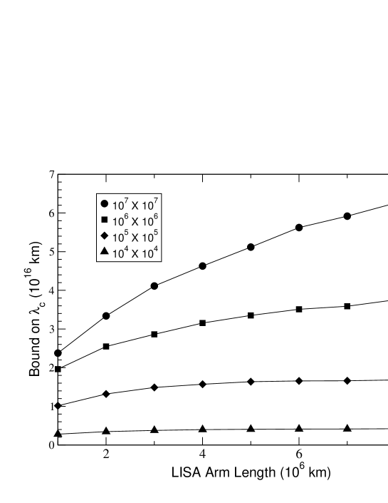
Figure 8: Bound on graviton compton wavelength $\lambda_{g}$ vs. LISA arm length for sources at $Z=1/2$; $5\times 10^{6}$ km is the baseline.

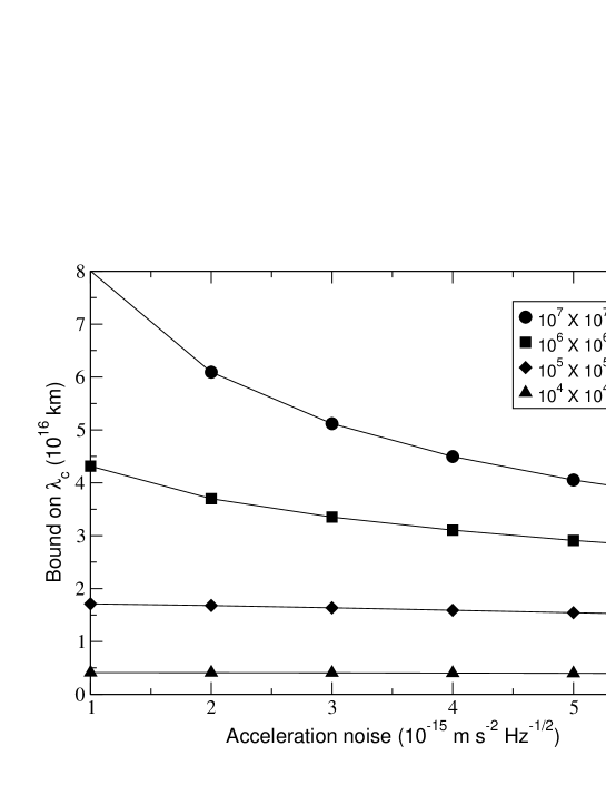
Figure 9: Bound on graviton compton wavelength $\lambda_{g}$ vs. LISA acceleration noise for sources at $Z=1/2$; $3\times 10^{-15}\,{\rm m}\,{\rm s}^{-2}\,{\rm Hz}^{-1/2}$ is the baseline.

The resulting bounds are in the range between $10^{15}$ and several $\times 10^{16}$ km. Figures 8 and 9 show the dependence of the bounds on LISA arm length $L$ and acceleration noise $A$. For the highest mass systems, the bounds vary as $L^{1/2}$, and $A^{-1/2}$ because the noise varies as $L^{-1}$ and $A$, while for the lower mass systems, there is little effect because the relevant signal is in the regime where WD confusion noise dominates over instrumental noise.

4 Discussion

We have used up-to-date LISA sensitivity curves from the SCG to refine the bounds that could be placed on alternative theories of gravity.

For scalar-tensor theory, the bound on $\omega$ could exceed that from the best current solar-system measurement, using the Cassini spacecraft, by factors of 10 and higher. For neutron star inspiral into a $400\,M_{\odot}$ black hole at 10 Mpc and a two-year integration, the bound could reach 2 million.

On the other hand, a number of alternative bounds on scalar-tensor gravity may reach levels competitive with these bounds on a comparable timescale. The gyroscope experiment Gravity Probe-B, set for launch in April 2004, anticipates placing a bound $\omega>10^{5}$ via measurement of the geodetic precession of gyroscopes orbiting in the curved spacetime around the Earth. Future space optical interferometery missions, such as GAIA, could reach comparable levels by measuring the deflection of light to microarcsecond precision. GAIA is planned for launch around the same time (2010) as LISA. The best hope for a dramatic improvement in $\omega$ bounds comes from the recently analysed binary pulsar system PSR J1141-6545, in which the companion is most likely a white dwarf [26]. Because of the asymmetry between the neutron star and white dwarf sensitivities (0.2 vs. $10^{-4}$), dipole gravitational radiation is significant, and a measurement of the rate of orbital decay ${\dot{P}}_{b}$ in agreement with GR at the one percent level could bound $\omega$ by as high as $10^{6}$ [27, 28]. Such a result could possibly be reached in a decade, the same timescale as LISA.

A major uncertainty in our proposed bound using LISA is the likelihood of observation of relatively nearby inspirals of a neutron star into intermediate mass black holes. Miller [29] has estimated the rate of inspirals of intermediate-mass binary black hole systems in globular clusters. For a $10\,M_{\odot}$ black hole inspiraling into a $100\,M_{\odot}$ black hole, Miller estimates yields a rate of one every 250 years, for one-year integrations. However one of us [33] has used the SCG to estimate a rate $7\times 10^{5}$ times lower. Whether these estimates apply to the neutron-star inspirals needed for scalar-tensor bounds is an open question at present. Although the rate may be low from the point of view of gravitational-wave astronomy, it is useful to point out that, to test alternative theories, a single serendipitous discovery is all it takes: witness the Hulse-Taylor binary pulsar.

Other methods have been suggested for bounding the graviton mass. We earlier showed that observations of binary inspiral using ground-based detectors of the advanced LIGO type could place a bound of several times $10^{12}$ km, comparable to the solar-system bound [3]. Sutton and Finn [30, 31] showed that, in a simple class of linearized massive graviton models, a bound comparable to or slightly better than the solar-system bound could be placed on $\lambda_{g}$ using binary pulsar data. Cutler, Hiscock and Larson [32] studied the effect of massive gravity on the observed gravitational-wave phase of known binary stars, compared to the orbital phase inferred from light measurements and showed that LISA observations could place bounds on $\lambda_{g}$ from 5 to 50 times larger than the current solar-system bound.

References

References

- [1] Danzmann K, for the LISA Science Team 1997 Class. Quantum Grav.14 1399
- [2] Will C M, 1994 Phys. Rev.D 50 6058 (Preprint gr-qc/9406022)
- [3] Will C M 1998 Phys. Rev.D 57 2061 (Preprint gr-qc/9709011)
- [4] Scharre P D and Will C M 2002 Phys. Rev.D 65 042002 (Preprint gr-qc/0109044)
- [5] Bertotti B, Iess L and Tortora P 2003 Nature 425 374
- [6] Babak S V and Grishchuk L P 1999 Phys. Rev.D 61 024038
- [7] Babak S V and Grishchuk L P 2003 Int. J. Mod. Phys. D 12 1905 (Preprint gr-qc/0209006)
- [8] Dvali G, Gabadadze G and Porrati M 2000 Phys. Lett. B 485 208 (Preprint hep-th/0005016)
- [9] Bender P, Ciufolini I, Danzmann K, Folkner W, Hough J, Robertson D, Rüdiger A, Sandford M, Schilling R, Schutz B, Stebbins R, Summer T, Touboul P, Vitale S, Ward H, and Winkler W 1995 LISA: Laser Interferometer Space Antenna for the Detection and Observation of Gravitational Waves, Pre-Phase A Report (unpublished)
- [10] Cutler C 1998 Phys. Rev.D 57 7089 (Preprint gr-qc/9703068)
- [11] Bender P L and Hils D 1997 Class. Quantum Grav.14 1439
- [12] Larson S L, Hiscock W A and Hellings R W 2001 Phys. Rev.D 62 062001 (Preprint gr-qc/9909080)
- [13] Armstrong J W, Estabrook F B and Tinto M 1999 Astrophys. J. 527 814
- [14] The Sensitivity Curve Generator was originally written by Shane Larson and may be found online at http://www.srl.caltech.edu/~shane/sensitivity/MakeCurve.html
- [15] Cutler C, Apostolatos T A, Bildsten L, Finn L S, Flanagan É E, Kennefick D, Marković D M, Ori A, Poisson E, Sussman G J and Thorne K S 1993 Phys. Rev. Lett.70 2984 (Preprint gr-qc/9208005)
- [16] Cutler C and Flanagan É E 1994 Phys. Rev.D 49 2658 (Preprint gr-qc/9402014)
- [17] Finn L S 1992 Phys. Rev.D 46 5236
- [18] Finn L S and Chernoff D F 1993 Phys. Rev.D 47 2198 (Preprint gr-qc/9301003)
- [19] Poisson E and Will C M 1995 Phys. Rev.D 52 848 (Preprint gr-qc/9502040)
- [20] Talmadge C, Berthias J-P, Hellings R W and Standish E M 1988 Phys. Rev. Lett.61 1159
- [21] Particle Data Group 1996 Review of Particle Properties, Phys. Rev.D 54 1
- [22] Blanchet L, Faye G, Iyer B R and Joguet B 2002 Phys. Rev.D 65 061501 (Preprint gr-qc/0105099)
- [23] Zakharov V I 1970 JETP Lett. 12 312
- [24] van Dam H and Veltman M 1970 Nucl. Phys. B22 397
- [25] Visser M 1998 Gen. Rel. Grav. 30 1717 (Preprint gr-qc/9705051)
- [26] Bailes M, Ord S M, Knight H S and Hotan A W 2003 Astrophys. J. Lett. 595 L49 (Preprint astro-ph/0307468)
- [27] Esposito-Farèse, G 2004 Proceedings of the 10th Marcel Grossmann Meeting, in press (Preprint gr-qc/0402007)
- [28] Gérard J-M and Wiaux Y 2002 Phys. Rev.D 66 024040 (Preprint gr-qc/0109062)
- [29] Miller M C 2002 Astrophys. J. 581 438 (Preprint astro-ph/0206404)
- [30] Finn L S and Sutton P J 2002 Phys. Rev.D 65 044022 (Preprint gr-qc/0109049)
- [31] Sutton P J and Finn L S 2002 Class. Quantum Grav.19 1355 (Preprint gr-qc/0112018)
- [32] Cutler C, Hiscock W A and Larson S L 2003 Phys. Rev.D 67 024015 (Preprint gr-qc/0209101)
- [33] Will C M 2004 (preprint)