Optimal combination of signals from co-located gravitational wave interferometers
for use in searches for a stochastic background

Abstract

This article derives an optimal  (i.e., unbiased, minimum variance) estimator for the pseudo-detector strain for a pair of co-located gravitational wave interferometers (such as the pair of LIGO interferometers at its Hanford Observatory), allowing for possible instrumental correlations between the two detectors. The technique is robust and does not involve any assumptions or approximations regarding the relative strength of gravitational wave signals in the Hanford pair with respect to other sources of correlated instrumental or environmental noise.

An expression is given for the effective power spectral density of the combined noise in the pseudo-detector. This can then be introduced into the standard optimal Wiener filter used to cross-correlate detector data streams in order to obtain an optimal estimate of the stochastic gravitational wave background. In addition, a dual  to the optimal estimate of strain is derived. This dual is constructed to contain no  gravitational wave signature and can thus be used as an “off-source” measurement to test algorithms used in the “on-source” observation.

I Introduction

Over the past few years a number of long-baseline interferometric gravitational wave detectors have begun operation. These include the Laser Interferometer Gravitational Wave Observatory (LIGO) detectors located in Hanford, WA and Livingston, LA ligoproject ; the GEO-600 detector near Hannover, Germany GEO-600 ; the VIRGO detector near Pisa, Italy virgo ; and the Japanese TAMA-300 detector in Tokyo tama . For the foreseeable future all these instruments will be looking for gravitational wave signals that are expected to be at the very limits of their sensitivities. All the collaborations have been developing data analysis techniques designed to extract weak signals from the detector noise. Coincidences among multiple detectors will be critical in establishing the first detections.

In particular, LIGO Laboratory operates two co-located detectors sharing a common vacuum envelope at its Hanford, WA Observatory (LHO). One of the two detectors has 4 km long arms and is denoted H1; the other, with 2 km long arms, is denoted H2. This pair is unique among all the other kilometer-scale interferometers in the world because their co-location guarantees simultaneous and essentially identical  responses to gravitational waves. This fact can provide a powerful discrimination tool for sifting true signals from detector noise. At the same time, however, the co-location of the detectors can allow for a greater level of correlated instrumental noise, complicating the analysis for gravitational waves.

Indeed, it may not be feasible to ever detect a stochastic gravitational wave background, or even establish a significant upper limit, via cross-correlation of H1 and H2, due to the potential of instrumental correlations. However, even though it may not be profitable to correlate these co-located detectors, the data from H1 and H2 should be optimally combined for a correlation analysis with a geographically separated third detector (such as L1, the LIGO Livingston detector).

For the H1-H2 detector pair, properly combining the two data streams will always result in a pseudo-strain channel that is quieter than the less noisy detector. In the limit of completely correlated noise, this combination could, in principal, lead to a noiseless estimate of gravitational wave strain. In the other limit where the detector noise is completely uncorrelated, the two detector outputs can of course be treated independently and combined at the end of the analysis to produce a more precise measurement than either separately, as done in Section V.C. of Ref. allenromano . It is the more general intermediate case, where there is partial correlation of the detector noise, that is the subject of this paper.

We show that it is possible to derive an optimal —i.e., unbiased, minimum variance—strain estimator by combining the two co-located interferometer outputs into a single, pseudo-detector  estimate of the gravitational wave strain from the observatory. An expression is given for the effective power spectral density of the combined noise in the pseudo-detector. This is then introduced into the standard optimal Wiener filter used to cross-correlate detector data streams in order to obtain an estimate of the stochastic gravitational wave background.

Once the optimal estimator is found, one can subtract this quantity from the individual interferometer strain channels, producing a pair of null  residual channels for the gravitational wave signature. The covariance matrix for these two null channels is Hermitian; it thus possesses two real eigenvalues and can be diagonalized by a unitary transformation (rotation). Because the covariance matrix is generated from a single vector, only one of the eigenvalues is non-zero. The corresponding eigenvector gives a single null channel that can be used as an “off-source” channel, which can be processed in the same manner as the optimal estimator of gravitational wave strain.

The technique described here is possible for the pair of Hanford detectors because, to high accuracy, the gravitational wave signature is guaranteed to be identical  in both instruments, and because we can identify specific correlations as being of instrumental origin. Coherent, time-domain mixing of the two interferometer strain channels can thus be used to optimal advantage to provide the best possible estimate of the gravitational wave strain, and to provide a null channel with which any gravitational wave analysis can be calibrated for backgrounds.

The focus of this paper is the development of this technique and its application to the search for stochastic gravitational waves. However, it appears that any other search can exploit this approach.

In Section II we discuss the experimental findings during recent LIGO science runs which motivated this work to extend the optimal filter formalism in the case where instrumental or environmental backgrounds are correlated among detectors. In Section III we introduce the optimal estimate of strain for the pair of co-located Hanford interferometers. In Section IV we then introduce the dual null channel. Then in Section V we apply these formalisms to measurement of a stochastic background and consider limiting cases that provide insight to understanding the concept. Finally in Section VI we discuss the implications of these results and estimate the effects of imperfect knowledge of calibrations on the technique. Appendices A, B contain derivations of formulae used in Sec. V.

II Instrumental correlations

Early operation at LIGO’s Hanford observatory has revealed that the two LHO detectors can exhibit instrumental cross-correlations of both narrowband and broadband nature. Narrowband correlations are found, e.g., at the $60$ Hz mains line frequency and harmonics, and at frequencies corresponding to clocks or timing signals common in the two detectors; these discrete frequencies can be identified and removed from the broadband analysis of a stochastic background search, as described in Ref. S1_stochpaper . Broadband instrumental correlations, on the other hand, are more pernicious to a stochastic background analysis; the following types of relatively broadband correlations have been seen at LHO:

• Low-frequency seismic excitation of the interferometer components, up to approximately 15 Hz; at higher frequencies, the seismic vibrations are not only greatly attenuated by the detectors’ isolation systems, but they also become uncorrelated over the distances separating the two interferometers. These correlations are not directly problematic, since they are below the detection band’s lower frequency of $40$ Hz.

• Acoustic vibrations of the output beam detection systems.

• Upconversion of seismic noise into the detector band: intermodulation between the mains line frequencies and the low-frequency seismic noise produces sidebands around the {60 Hz, 120 Hz, …} lines that are correlated between the two detectors.

Magnetic field coupling to the detectors is another potential source of correlated noise, though this has not yet been seen to be significant.

The analysis of the first LIGO science data (S1) for a stochastic gravitational wave background S1_stochpaper showed substantial cross-correlated noise between the two Hanford interferometers (H1 and H2), due to the above sources. This observation led to disregarding the H1-H2 cross-correlation measurement as an estimate of the stochastic background signal strength. Two separate upper limits were obtained for the two transcontinental pairs, L1-H1 and L1-H2 (L1 denotes the 4 km LIGO interferometer in Livingston, LA). These were not combined because of the known cross-correlation contaminating the H1-H2 pair.

Here, we show how to take into account such local instrumental correlations in an optimal fashion by first combining the two local interferometer strain channels into a single, pseudo-detector estimate of the gravitational wave strain from the Hanford site, and then cross-correlating this pseudo-detector channel with the single Livingston detector output. In doing this, we obtain a self-consistent utilisation of the three measurements to obtain a single  estimate of the stochastic background signal strength $\Omega_{\rm gw}$. In order for this to be valid, the reasonable assumption is made that there are no broadband transcontinental (i.e., L1-H1, L1-H2) instrumental or environmental correlations. This has been empirically observed to be the case for the S1, S2 and S3 science runs when the L1-H1 and L1-H2 coherences are calculated over long periods of time (the S1 findings are discussed in S1_stochpaper ; S2 and S3 analyses are still in progress at the time of this writing).

It is important to point out that the technique presented here is robust and does not involve any assumptions or approximations regarding the relative strength of gravitational wave signals in the H1-H2 pair with respect to other sources of correlated instrumental or environmental noise. Since S1, the sources of environmental correlation between the Hanford pair have been largely reduced or eliminated. However, as the overall detector noise is also reduced, smaller cross-correlations become significant, so it remains important to be able to optimally exploit the potential sensitivity provided by this unique pair of co-located detectors.

III Optimal estimate of strain for the two Hanford detectors

Assume that the detectors H1 and H2 produce data streams

$$s_{H_{1}}(t) := h(t)+n_{H_{1}}(t)\,,$$ (1)

$$s_{H_{2}}(t) := h(t)+n_{H_{2}}(t)\,,$$ (2)

respectively, where $h(t)$ is the gravitational wave strain common to both the detectors. In the Fourier domain,

$$\widetilde{s}_{H_{1}}(f) = \widetilde{h}(f)+\widetilde{n}_{H_{1}}(f)\,,$$ (3)

$$\widetilde{s}_{H_{2}}(f) = \widetilde{h}(f)+\widetilde{n}_{H_{2}}(f)\,,$$ (4)

where we defined the Fourier transform of a time domain function, $a(t)$, as $\widetilde{a}(f):=\int_{-\infty}^{\infty}dt\,e^{-i2\pi ft}\,a(t)$. Also assume that the processes generating $h$, $n_{H_{1}}$, $n_{H_{2}}$ are stochastic with the following statistical properties:

$$\langle\widetilde{n}_{H_{i}}(f)\rangle=\langle\widetilde{h}(f)\rangle = 0\,,$$ (5)

$$\langle\widetilde{n}_{H_{i}}^{*}(f)\widetilde{h}(f)\rangle = 0\,,$$ (6)

$$\langle\widetilde{n}_{H_{i}}^{*}(f)\widetilde{n}_{H_{j}}(f^{\prime})\rangle = P^{n}_{H_{i}H_{j}}(f)\,\delta(f-f^{\prime})\,,$$ (7)

$$\langle\widetilde{h}^{*}(f)\widetilde{h}(f^{\prime})\rangle = P_{\Omega}(f)\,\delta(f-f^{\prime})\,,$$ (8)

$$\langle\widetilde{s}_{H_{i}}^{*}(f)\widetilde{s}_{H_{j}}(f^{\prime})\rangle := P_{H_{i}H_{j}}(f)\,\delta(f-f^{\prime})\,$$ (9)

$$= (P^{n}_{H_{i}H_{j}}(f)+P_{\Omega}(f))\,$$ (11)

$$\times\delta(f-f^{\prime})$$

$$P^{n}_{H_{i}H_{i}}(f) := P^{n}_{H_{i}}(f)\,,$$ (12)

$$P_{H_{i}H_{i}}(f) := P_{H_{i}}(f)\,,$$ (13)

$$\rho_{H_{i}H_{j}}(f) := \frac{P_{H_{i}H_{j}}(f)}{\sqrt{P_{H_{i}}(f)P_{H_{j}}(f)}}\,,$$ (14)

$$\Gamma_{H_{i}H_{j}}(f) := |\rho_{H_{i}H_{j}}(f)|^{2}\,,$$ (15)

$$P_{\Omega}(f) \ll P_{H_{i}}(f)\,,$$ (16)

where $i=1,2$ and the angular brackets $\langle...\rangle$ denote ensemble or statistical averages of random processes. Note that Eqs. (9) and (13) signify the measurable cross-power and power spectra while Eqs. (7) and (12) refer to intrinsic noise quantities that cannot, in principle, be isolated in a measurement. Often, Eq. (16) is assumed in order to identify instrument noise power with the measured quantity. Note also that the coherence $\rho_{H_{i}H_{j}}(f)$ is a complex quantity of magnitude less than or equal to unity, and that $P_{H_{j}H_{i}}(f)=P^{*}_{H_{i}H_{j}}(f)$.

Now construct an unbiased  linear combination of $\widetilde{s}_{H_{i}}(f)$:

$$\widetilde{s}_{H}(f):=\widetilde{\alpha}(f)\widetilde{s}_{H_{1}}(f)+(1-\widetilde{\alpha}(f))\widetilde{s}_{H_{2}}(f)\,.$$ (17)

If $\widetilde{s}_{H}(f)$ is also to be a minimum variance  estimator, where

$${\rm Var}(s_{H}):=\langle\widetilde{s}^{*}_{H}(f)\widetilde{s}_{H}(f^{\prime})\rangle=P_{H}(f)\,\delta(f-f^{\prime})\,,$$ (18)

with

$$P_{H}(f) = |\widetilde{\alpha}(f)|^{2}P^{n}_{H_{1}}(f)+|1-\widetilde{\alpha}(f)|^{2}P^{n}_{H_{2}}(f)+$$

$$+\widetilde{\alpha}^{*}(f)(1-\widetilde{\alpha}(f))P^{n}_{H_{1}H_{2}}(f)+$$

$$+\widetilde{\alpha}(f)(1-\widetilde{\alpha}^{*}(f))P^{n*}_{H_{1}H_{2}}(f)+P_{\Omega}(f)\,,$$

then $\widetilde{\alpha}(f)$ must have the following form:

$$\widetilde{\alpha}(f)=\frac{P_{H_{2}}(f)-P_{H_{1}H_{2}}(f)}{P_{H_{1}}(f)+P_{H_{2}}(f)-(P_{H_{1}H_{2}}(f)+P^{*}_{H_{1}H_{2}}(f))}\,.$$ (20)

The corresponding power of the pseudo-detector signal is

$$P_{H}(f)=\frac{P_{H_{1}}(f)P_{H_{2}}(f)(1-\Gamma_{H_{1}H_{2}}(f))}{P_{H_{1}}(f)+P_{H_{2}}(f)-(P_{H_{1}H_{2}}(f)+P^{*}_{H_{1}H_{2}}(f))}\,.$$ (21)

It is important to note that the above expressions for $\widetilde{\alpha}(f)$ and $P_{H}(f)$ do not  require any assumption on the relative strength of the cross-correlated stochastic signal to the instrumental or environmental cross-correlated noise. In particular, the stochastic signal power $P_{\Omega}$ enters $P_{H_{1}}$, $P_{H_{2}}$, and $P_{H_{1}H_{2}}$ in exactly the same way, canceling out in Eq. (20), implying that the above solution for $\widetilde{\alpha}$ is independent of the relative strength of the stochastic signal to other sources of cross-correlated noise. In addition, Eqs. (20), (21) involve only experimentally measurable  power spectra and cross-spectra (and not the intrinsic noise spectra), indicating that this procedure can be carried out in practice.

Figure 1 shows plots of the strain spectral densities for $\widetilde{s}_{H}(f)$, $\widetilde{s}_{H_{1}}(f)$, and $\widetilde{s}_{H_{2}}(f)$, representative of the S1 data.

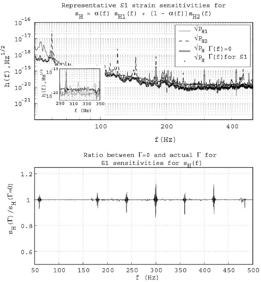
Figure 1: Strain spectral densities (i.e., absolute value) of $\widetilde{s}_{H}(f)$ (gray or dotted), $\widetilde{s}_{H_{1}}(f)$ (black), and $\widetilde{s}_{H_{2}}(f)$ (dashed), representative of the S1 data. Top Panel: overlay of the individual spectral densities with that of the strain spectral density $|\widetilde{s}_{H}(f)|$ calculated with the S1 run-averaged coherence, $\Gamma_{H_{1}H_{2}}(f)$, and with $\Gamma_{H_{1}H_{2}}(f)=0$. On this scale, the left hand panel shows no discernible difference between the spectra for $\Gamma_{H_{1}H_{2}}(f)$, and with $\Gamma_{H_{1}H_{2}}(f)=0$, suggesting that even the level of coherence seen during the S1 run might be sufficiently low to allow one to simply combine the L1-H1 and L2-H2 cross-correlation measurements under the assumption of zero cross-correlated noise. The optimality of the estimate $\widetilde{s}_{H}(f)$ is visible here because it is always less than the smaller  of $\widetilde{s}_{H_{1}}(f)$ or $\widetilde{s}_{H_{2}}(f)$. The inset shows a blow-up of the region near one of the spectral features. On this scale the individual spectra can be discerned. Bottom panel: plot of the ratio of amplitude spectra for $|\widetilde{s}_{H}(f)|$ calculated with $\Gamma_{H_{1}H_{2}}(f)$ as measured during S1 and $\Gamma_{H_{1}H_{2}}(f)=0$ (i.e., assuming no coherence). The difference between the two is very small except for the very lowest frequencies and at narrow line features.

The strain spectral density $|\widetilde{s}_{H}(f)|$ is calculated from Eqs. (17) and (20) for both $\Gamma_{H_{1}H_{2}}(f)=0$ (i.e., an artificial case that assumes no coherence), and for the coherence $\Gamma_{H_{1}H_{2}}(f)$ that was actually measured over the whole S1 data run (see Fig. 2). The plots in Fig. 1 suggest that the observed level of coherence during the S1 run, $\Gamma\sim 10^{-5}$, might be sufficiently low that one can simply combine the L1-H1, L1-H2 cross-correlation measurements under the assumption of zero cross-correlated noise (c.f. Eq. (73)). The formalism developed in this paper allows a quantitative assessment of the effect of instrumental or environmental correlations on combining independently analyzed results ex post facto.

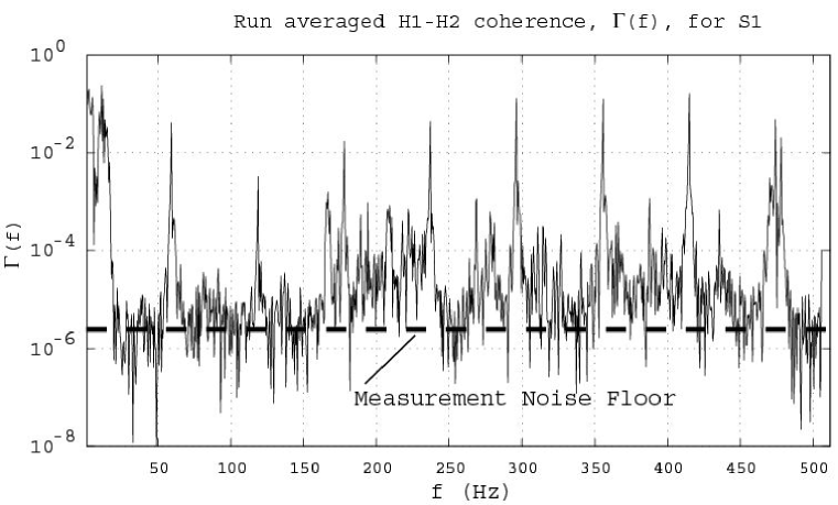
Figure 2: H1-H2 coherence averaged over the whole S1 data run. Note the substantial broadband coherence below 250 Hz and between 400 and 475 Hz. Low frequency seismic noise and acoustic coupling between the input electro-optics systems are considered to be the prime sources of this cross-correlated noise S1_stochpaper ; schofield .

III.1 Limiting cases

I. If $\rho_{H_{1}H_{2}}(f)=0$, then

$$\widetilde{\alpha}(f) = \frac{P_{H_{2}}(f)}{P_{H_{1}}(f)+P_{H_{2}}(f)}\,,$$ (22)

$$\widetilde{s}_{H}(f) = \frac{P_{H_{2}}(f)\widetilde{s}_{H_{1}}(f)+P_{H_{1}}(f)\widetilde{s}_{H_{2}}(f)}{P_{H_{1}}(f)+P_{H_{2}}(f)}\,,$$ (23)

$$P_{H}(f) = \frac{P_{H_{1}}(f)P_{H_{2}}(f)}{P_{H_{1}}(f)+P_{H_{2}}(f)}\,.$$ (24)

II. If $P_{H_{1}}(f)=P_{H_{2}}(f)$, then

$$\widetilde{\alpha}(f)=\frac{1-\rho_{H_{1}H_{2}}(f)}{2-(\rho_{H_{1}H_{2}}(f)+\rho_{H_{1}H_{2}}^{*}(f))}\,.$$ (25)

III. If $\rho_{H_{1}H_{2}}(f)=1$ and $P_{H_{1}}(f)=P_{H_{2}}(f)$, then

$$P_{H}(f)=\lim_{\Gamma(f)\rightarrow 1}{\frac{P_{H_{1}}(f)}{2}}\frac{1-\Gamma(f)}{1-\sqrt{\Gamma(f)}}=P_{H_{1}}(f)\,.$$ (26)

IV. If $P_{H_{2}}(f)=4P_{H_{1}}(f)$ (which is the limiting design performance for H1 and H2 due to the $2:1$ arm length ratio), then

$$\widetilde{\alpha}(f)=\frac{2(2-\rho_{H_{1}H_{2}}(f))}{5-2(\rho_{H_{1}H_{2}}(f)+\rho_{H_{1}H_{2}}^{*}(f))}\,.$$ (27)

Note for this case that if the noise were either completely correlated ($\rho_{H_{1}H_{2}}(f)=1\Rightarrow\widetilde{\alpha}(f)=2$) or anti-correlated ($\rho_{H_{1}H_{2}}(f)=-1\Rightarrow\widetilde{\alpha}(f)=2/3$), then one could exactly cancel the noise from the signals $\widetilde{s}_{H_{i}}$. If the noise is uncorrelated ($\rho_{H_{1}H_{2}}(f)=0\Rightarrow\widetilde{\alpha}(f)=4/5$), then the weighting of the signals from the two interferometers is in the ratio $4:1$, as expected.

IV A dual to the optimal estimate of strain that cancels the gravitational wave signature

In the previous section, an optimal estimator of the gravitational wave strain $h$ was derived by appropriately combining the outputs of the two Hanford detectors. It is also possible to form a dual  to this optimal estimate (denoted $\widetilde{z}_{H}(f)$) that explicitly cancels the gravitational wave signature.

Starting with Eqs. (3), (4), and the optimal estimate $\widetilde{s}_{H}(f)$, we construct the $h$-subtracted residuals:

$$\widetilde{z}_{H_{1}}(f) := \widetilde{s}_{H_{1}}(f)-\widetilde{s}_{H}(f)\,,$$ (28)

$$\widetilde{z}_{H_{2}}(f) := \widetilde{s}_{H_{2}}(f)-\widetilde{s}_{H}(f)\,.$$ (29)

Both $\widetilde{z}_{H_{1}}(f)$, $\widetilde{z}_{H_{2}}(f)$ are proportional to $\widetilde{n}_{H_{1}}(f)-\widetilde{n}_{H_{2}}(f)$, although with different frequency-dependent weighting functions:

$$\widetilde{z}_{H_{1}}(f) = \left(1-\widetilde{\alpha}(f)\right)\,\left(\widetilde{n}_{H_{1}}(f)-\widetilde{n}_{H_{2}}(f)\right)\,,$$ (30)

$$\widetilde{z}_{H_{2}}(f) = -\widetilde{\alpha}(f)\,\left(\widetilde{n}_{H_{1}}(f)-\widetilde{n}_{H_{2}}(f)\right)\,.$$ (31)

Figure 3 shows schematically the geometrical relationships of the signal vectors $\widetilde{s}_{H_{i}}(f)$ and $\widetilde{z}_{H_{i}}(f)$.

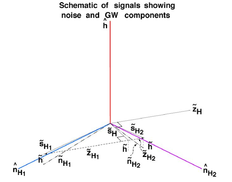
Figure 3: Schematic showing how the H1 and H2 signals may be represented in a 3-dimensional space of noise components for the two detectors and the common gravitational wave strain: {$\hat{n}_{H_{1}},\hat{n}_{H_{2}},\hat{h}$}. The signals $\widetilde{s}_{H_{1}}(f)$ and $\widetilde{s}_{H_{2}}(f)$ are not, in general, orthogonal if the coherence between the noise, $\widetilde{n}_{H_{1}}(f)$ and $\widetilde{n}_{H_{2}}(f)$, is non-zero. $\widetilde{s}_{H}(f)$ is the minimum variance estimate of $\widetilde{h}(f)$ derived from $\widetilde{s}_{H_{1}}(f)$ and $\widetilde{s}_{H_{2}}(f)$. Using $\widetilde{s}_{H}(f)$ as the best estimate of $\widetilde{h}(f)$, this signal can be subtracted from $\widetilde{s}_{H_{1}}(f)$ and $\widetilde{s}_{H_{2}}(f)$ to produce the vectors $\widetilde{z}_{H_{1}}(f)$, $\widetilde{z}_{H_{2}}(f)$ that lie in the $\hat{n}_{H_{1}}$-$\hat{n}_{H_{2}}$ plane. These vectors give rise to the covariance matrix $||\widetilde{\bf{C}}_{z}(f)||$. $\widetilde{z}_{H_{1}}(f)$ and $\widetilde{z}_{H_{2}}(f)$ are colinear and thus one of the eigenvectors of $||\widetilde{\bf{C}}_{z}(f)||$ will be zero. The other corresponds to the dual of $\widetilde{s}_{H}(f)$, denoted $\widetilde{z}_{H}(f)$, which is orthogonal to $\widetilde{s}_{H}(f)$, as shown in the figure. Note that it is necessary to first subtract the contribution of $\widetilde{h}(f)$ from the signals before forming the covariance matrix.

Once the best estimate $\widetilde{s}_{H}(f)$ is subtracted from the signals, the residuals lie in the $\hat{n}_{H_{1}}$-$\hat{n}_{H_{2}}$ plane. (Here $\hat{n}_{H_{1}}$ and $\hat{n}_{H_{2}}$ are unit vectors pointing in directions corresponding to uncorrelated  detector noise.) Their covariance matrix can then be diagonalized without affecting the gravitational wave signature $h$ contained in $\widetilde{s}_{H}(f)$.

Now consider the covariance matrix

$$||\widetilde{\bf C}_{z}||_{ij}\,\delta(f-f^{\prime}):=\langle\widetilde{z}^{*}_{H_{i}}(f)\widetilde{z}_{H_{j}}(f^{\prime})\rangle\,.$$ (32)

Then one can show that

$$||\widetilde{\bf C}_{z}(f||\,\delta(f-f^{\prime}) = \left[\begin{array}[]{c c}\langle\widetilde{z}^{*}_{H_{1}}(f)\widetilde{z}_{H_{1}}(f^{\prime})\rangle&\langle\widetilde{z}^{*}_{H_{1}}(f)\widetilde{z}_{H_{2}}(f^{\prime})\rangle\\ \langle\widetilde{z}^{*}_{H_{2}}(f)\widetilde{z}_{H_{1}}(f^{\prime})\rangle&\langle\widetilde{z}^{*}_{H_{2}}(f)\widetilde{z}_{H_{2}}(f^{\prime})\rangle\end{array}\right]$$ (35)

$$= \left[\begin{array}[]{c c}|1-\widetilde{\alpha}(f)|^{2}&-\widetilde{\alpha}(f)+|\widetilde{\alpha}(f)|^{2}\\ -\widetilde{\alpha}^{*}(f)+|\widetilde{\alpha}(f)|^{2}&|\widetilde{\alpha}(f)|^{2}\end{array}\right]\langle(\widetilde{n}^{*}_{H_{1}}(f)-\widetilde{n}^{*}_{H_{2}}(f))(\widetilde{n}_{H_{1}}(f^{\prime})-\widetilde{n}_{H_{2}}(f^{\prime}))\rangle$$ (38)

$$= \left[\begin{array}[]{c c}|1-\widetilde{\alpha}(f)|^{2}&-\widetilde{\alpha}(f)+|\widetilde{\alpha}(f)|^{2}\\ -\widetilde{\alpha}^{*}(f)+|\widetilde{\alpha}(f)|^{2}&|\widetilde{\alpha}(f)|^{2}\end{array}\right]\langle(\widetilde{s}^{*}_{H_{1}}(f)-\widetilde{s}^{*}_{H_{2}}(f))(\widetilde{s}_{H_{1}}(f^{\prime})-\widetilde{s}_{H_{2}}(f^{\prime}))\rangle$$ (41)

$$= \left[\begin{array}[]{c c}|1-\widetilde{\alpha}(f)|^{2}&-\widetilde{\alpha}(f)+|\widetilde{\alpha}(f)|^{2}\\ -\widetilde{\alpha}^{*}(f)+|\widetilde{\alpha}(f)|^{2}&|\widetilde{\alpha}(f)|^{2}\end{array}\right]\times$$ (45)

$$\times\left(P_{H_{1}}(f)+P_{H_{2}}(f)-(P_{H_{1}H_{2}}(f)+P^{*}_{H_{1}H_{2}}(f))\right)\,\delta(f-f^{\prime})\,.$$

Diagonalization of $||\widetilde{\bf{C}}_{z}(f)||$ gives the eigenvalues:

$$\lambda_{1} = 0\,,$$ (46)

$$\lambda_{2} = \left(P_{H_{1}}(f)+P_{H_{2}}(f)-(P_{H_{1}H_{2}}(f)+P^{*}_{H_{1}H_{2}}(f))\right)\,\left(1-\widetilde{\alpha}(f)-\widetilde{\alpha}^{*}(f)+2|\widetilde{\alpha}(f)|^{2}\right)\,.$$ (47)

The non-trivial solution corresponds to the desired “zero” pseudo-detector channel:

$$\widetilde{z}_{H}(f)=-\left(\widetilde{s}_{H_{1}}(f)-\widetilde{s}_{H_{2}}(f)\right)\,\sqrt{1-\widetilde{\alpha}(f)-\widetilde{\alpha}^{*}(f)+2|\widetilde{\alpha}(f)|^{2}}\,,$$ (48)

where $\widetilde{\alpha}(f)$ is given as before (c.f. Eq. (20)). The power spectrum $P_{z}(f)$ of $\widetilde{z}_{H}(f)$ is given by the eigenvalue $\lambda_{2}$ above.

Figure 4 shows plots of the strain spectral densities for $\widetilde{z}_{H}(f)$, $\widetilde{s}_{H_{1}}(f)$, and $\widetilde{s}_{H_{2}}(f)$, representative of the S1 data, similar to Fig. 1.

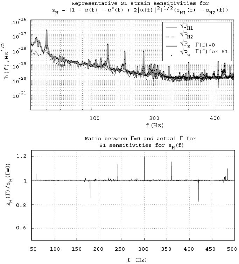
Figure 4: Same as Fig. 1, but for the null signal $\widetilde{z}_{H}(f)$ instead of the optimal estimate $\widetilde{s}_{H}(f)$. Strain spectral densities (i.e., absolute value) of $\widetilde{z}_{H}(f)$ (gray or dotted), $\widetilde{s}_{H_{1}}(f)$ (black), and $\widetilde{s}_{H_{2}}(f)$ (dashed), representative of the S1 data. Top Panel: overlay of the individual amplitude spectral densities with that of the strain spectral density $|\widetilde{z}_{H}(f)|$ is calculated with the S1 run-averaged coherence, $\Gamma_{H_{1}H_{2}}(f)$. On this scale, the left hand panel shows no discernible difference between the spectra for $\Gamma_{H_{1}H_{2}}(f)$, and with $\Gamma_{H_{1}H_{2}}=0$, suggesting that even the level of coherence seen during the S1 run might be sufficiently low to allow one to simply combine the L1-H1 and L2-H2 cross-correlation measurements under the assumption of zero cross-correlated noise. The optimality of the estimate $\widetilde{z}_{H}(f)$ is visible here because it is always less than the larger of $\widetilde{s}_{H_{1}}(f)$ or $\widetilde{s}_{H_{2}}(f)$. Bottom panel: overlay of individual amplitude spectra with that for $|\widetilde{z}_{H}(f)|$ calculated with $\Gamma_{H_{1}H_{2}}(f)=0$ (i.e., assuming no coherence). The difference between the two is very small except for the very lowest frequencies and at narrow line features.

IV.1 Limiting case for zero cross-correlated noise

In the limit that the two detectors are uncorrelated (i.e., $\rho_{H_{1}H_{2}}(f)=0$), the expression for $\widetilde{\alpha}(f)$ simplifies considerably (c.f. Eq. (22)). In this limit, $\widetilde{z}_{H}(f)$ and $P_{z}(f)$ become

$$\widetilde{z}_{H}(f) = -\left(\widetilde{s}_{H_{1}}(f)-\widetilde{s}_{H_{2}}(f)\right)\frac{\sqrt{P^{2}_{H_{1}}(f)+P^{2}_{H_{2}}(f)}}{P_{H_{1}}(f)+P_{H_{2}}(f)}\,,$$

$$P_{z}(f) = \frac{P^{2}_{H_{1}}(f)+P^{2}_{H_{2}}(f)}{P_{H_{1}}(f)+P_{H_{2}}(f)}\,.$$ (50)

In particular, note that $P_{z}(f)$ satisfies the inequality

$$\max\{P_{H_{1}}(f),P_{H_{2}}(f)\}-\min\{P_{H_{1}}(f),P_{H_{2}}(f)\}$$

$$\leq P_{z}(f)\leq\max\{P_{H_{1}}(f),P_{H_{2}}(f)\}\,.$$ (51)

This last equation shows that the null channel $\widetilde{z}_{H}(f)$ contains less  noise power than the difference of $\widetilde{n}_{H_{1}}(f)$, $\widetilde{n}_{H_{2}}(f)$. The filtering produced by $\widetilde{\alpha}(f)$ results in a less noisy null estimator than the quantity $\widetilde{n}_{H_{1}}(f)-\widetilde{n}_{H_{2}}(f)$. In the limit that either signal dominates the noise power (e.g., $P_{H_{1}}(f)\ll P_{H_{2}}(f)$),

$$P_{z}(f)\rightarrow\max\{P_{H_{1}}(f),P_{H_{2}}(f)\}-\min\{P_{H_{1}}(f),P_{H_{2}}(f)\}\,.$$ (52)

In addition, one can form the quantity:

$$t(f):=\frac{\widetilde{z}_{H}(f)}{\sqrt{P_{z}(f)}}=\frac{-\left(\widetilde{s}_{H_{1}}(f)-\widetilde{s}_{H_{2}}(f)\right)}{\sqrt{P_{H_{1}}(f)+P_{H_{2}}(f)}}.$$ (53)

As suggested by the label $t$, this quantity is identical to the Student’s $t$ statistic, which is used to assess the statistical significance of two quantities having different means and variances.

V Cross-correlation statistics using composite pseudo-detector channels

Since the instrumental transcontinental (L1-H1, L1-H2) cross-correlations are assumed to be negligible, the derivation of the optimal filter when using the pseudo-detector channels for Hanford proceeds exactly as has been presented in the literature flan ; leshouches ; allenromano with $P_{H_{1}}(f)$, $P_{H_{2}}(f)$ replaced by $P_{H}(f)$, $P_{z}(f)$ for the optimal estimate and the null signal, respectively.

V.1 Cross-correlation statistic for the optimal estimate of the gravitational wave strain

The cross-correlation statistic is given by

$$Y_{L_{1}H}:=\int_{-T/2}^{T/2}dt_{1}\int_{-T/2}^{T/2}dt_{2}\,s_{L_{1}}(t_{1})\,Q_{L_{1}H}(t_{1}-t_{2})\,s_{H}(t_{2})\,,$$ (54)

where $T$ is the observation time and $Q_{L_{1}H}(t)$ is the optimal  filter, which is chosen to maximize the signal-to-noise ratio of $Y_{L_{1}H}$. The corresponding frequency domain expression is

$$Y_{L_{1}H}\propto\int_{-\infty}^{\infty}df\,\widetilde{s}_{L_{1}}^{*}(f)\,\widetilde{Q}_{L_{1}H}(f)\,\widetilde{s}_{H}(f)\,.$$ (55)

Specializing to the case $\Omega_{\rm gw}(f)\equiv\Omega_{0}={\rm const}$, the optimal filter becomes

$$\widetilde{Q}_{L_{1}H}(f)={\cal N}_{L_{1}H}\frac{\gamma(|f|)}{|f|^{3}P_{L_{1}}(f)P_{H}(f)}\,,$$ (56)

where ${\cal N}_{L_{1}H}$ is a (real) overall normalization constant. In practice we choose ${\cal N}_{L_{1}H}$ so that the expected value of the cross-correlation is $\Omega_{0}\,h_{100}^{2}\,T$, where $h_{100}$ is the Hubble expansion rate $H_{0}$ in units of $H_{100}:=100~{}{\rm km}\,\,{\rm s}^{-1}\,{\rm Mpc}^{-1}$. For such a choice,

$${\cal N}_{L_{1}H}=\frac{20\pi^{2}}{3H_{100}^{2}}\ \left[\int_{-\infty}^{\infty}df\,\frac{\gamma^{2}(|f|)}{f^{6}P_{L_{1}}(f)P_{H}(f)}\right]^{-1}\,.$$ (57)

Moreover, one can show that the normalization factor ${\cal N}_{L_{1}H}$ and theoretical variance, $\sigma^{2}_{Y_{L_{1}H}}$, of $Y_{L_{1}H}$ are related by a simple numerical factor:

$${\cal N}_{L_{1}H}=\frac{1}{T}\left(\frac{3H^{2}_{100}}{5\pi^{2}}\right)\sigma^{2}_{Y_{L_{1}H}}\,.$$ (58)

V.1.1 Limiting case for white coherence and $P_{H_{1}}(f)\propto P_{H_{2}}(f)$

If the coherence is white (i.e., $\rho_{H_{1}H_{2}}(f)={\rm const}$) and the power spectra $P_{H_{1}}(f)$, $P_{H_{2}}(f)$ are proportional to one another, then one can show that the value of the cross-correlation statistic $Y_{L_{1}H}$ reduces to a linear combination of the cross-correlation statistics $Y_{L_{1}H_{1}}$ and $Y_{L_{1}H_{2}}$ calculated separately for L1-H1 and L1-H2, if we allow for instrumental correlations between H1 and H2. Thus, for this case, combining the point estimates of $\Omega_{0}$ made separately for L1-H1 and L1-H2 gives the same result as performing the coherent pseudo-detector channel analysis using the single optimal estimator $\widetilde{s}_{H}(f)$.

To show that this is indeed the case, note that $\rho_{H_{1}H_{2}}(f)={\rm const}$ implies

$$\Gamma_{H_{1}H_{2}}(f):=\left|\rho_{H_{1}H_{2}}(f)\right|^{2}={\rm const}\,.$$ (59)

We will drop subscripts for constant quantities. If we further assume that $P_{H_{2}}(f)=\eta P_{H_{1}}(f)$, then

$$\frac{P_{H_{1}H_{2}}(f)}{P_{H_{2}}(f)}=\frac{\rho}{\sqrt{\eta}}\,,\quad\frac{P^{*}_{H_{1}H_{2}}(f)}{P_{H_{1}}(f)}=\rho^{*}\sqrt{\eta}\,.$$ (60)

Thus, the integrand of the cross-correlation statistic,

$$Y_{L_{1}H}(f):=\widetilde{s}^{*}_{L_{1}}(f)\,\widetilde{Q}_{L_{1}H}(f)\,\widetilde{s}_{H}(f)\,,$$ (61)

becomes

$$\frac{Y_{L_{1}H}(f)}{{\cal N}_{L_{1}H}} = \frac{\gamma(f)\widetilde{s}^{*}_{L_{1}}(f)\left[\widetilde{s}_{H_{1}}(f)(P_{H_{2}}(f)-P_{H_{1}H_{2}}(f))+\widetilde{s}_{H_{2}}(f)(P_{H_{1}}(f)-P^{*}_{H_{1}H_{2}}(f))\right]}{|f|^{3}P_{L_{1}}(f)P_{H_{1}}(f)P_{H_{2}}(f)\,(1-\Gamma_{H_{1}H_{2}}(f))}$$ (62)

$$= \frac{1}{1-\Gamma}\,\left[\left(1-\frac{\rho}{\sqrt{\eta}}\right)\,\frac{Y_{L_{1}H_{1}}(f)}{{\cal N}_{L_{1}H_{1}}}+\left(1-\rho^{*}\sqrt{\eta}\right)\,\frac{Y_{L_{1}H_{2}}(f)}{{\cal N}_{L_{1}H_{2}}}\right]\,,$$ (63)

where the normalization factor Eq. (57) is

$${\cal N}_{L_{1}H} = \frac{20\pi^{2}}{3H_{100}^{2}}\left[\int_{-\infty}^{\infty}df\,\frac{\gamma^{2}(|f|)(P_{H_{1}}(f)+P_{H_{2}}(f)-(P_{H_{1}H_{2}}(f)+P^{*}_{H_{1}H_{2}}(f)))}{f^{6}P_{L_{1}}(f)P_{H_{1}}(f)P_{H_{2}}(f)\,(1-\Gamma_{H_{1}H_{2}}(f))}\right]^{-1}$$ (64)

$$= (1-\Gamma)\,\left[\left(1-\frac{\rho}{\sqrt{\eta}}\right)\,{\cal N}_{L_{1}H_{1}}^{-1}+\left(1-\rho^{*}\sqrt{\eta}\right)\,{\cal N}_{L_{1}H_{2}}^{-1}\right]^{-1}\,.$$ (65)

Equivalently,

$$\sigma_{Y_{L_{1}H}}^{2} = (1-\Gamma)\,\left[\left(1-\frac{\rho}{\sqrt{\eta}}\right)\,\sigma^{-2}_{Y_{L_{1}H_{1}}}+\left(1-\rho^{*}\sqrt{\eta}\right)\,\sigma^{-2}_{Y_{L_{1}H_{2}}}\right]^{-1}$$ (66)

$$= (1-\Gamma)\,\frac{\sigma^{2}_{Y_{L_{1}H_{1}}}\sigma^{2}_{Y_{L_{1}H_{2}}}}{\sigma^{2}_{Y_{L_{1}H_{1}}}\left(1-\rho^{*}\sqrt{\eta}\right)+\sigma^{2}_{Y_{L_{1}H_{2}}}\left(1-\frac{\rho}{\sqrt{\eta}}\right)\,,}$$ (67)

where we used Eq. (58) and similar equations to relate ${\cal N}_{L_{1}H_{1}}$, ${\cal N}_{L_{1}H_{2}}$ to $\sigma^{2}_{L_{1}H_{1}}$, $\sigma^{2}_{L_{1}H_{2}}$.

Substituting the above results for the normalization factors and variances into Eq. (63) and integrating over frequency, we find:

$$Y_{L_{1}H} = \frac{\sigma_{Y_{L_{1}H}}^{2}}{(1-\Gamma)}\,\left[\left(1-\frac{\rho}{\sqrt{\eta}}\right)\,\frac{Y_{L_{1}H_{1}}}{\sigma^{2}_{Y_{L_{1}H_{1}}}}+\left(1-\rho^{*}\sqrt{\eta}\right)\,\frac{Y_{L_{1}H_{2}}}{\sigma^{2}_{Y_{L_{1}H_{2}}}}\right]$$ (68)

$$= \frac{\sigma^{2}_{Y_{L_{1}H_{1}}}\sigma^{2}_{Y_{L_{1}H_{2}}}}{\sigma^{2}_{Y_{L_{1}H_{1}}}\left(1-\rho^{*}\sqrt{\eta}\right)+\sigma^{2}_{Y_{L_{1}H_{2}}}\left(1-\frac{\rho}{\sqrt{\eta}}\right)}\,\left[\left(1-\frac{\rho}{\sqrt{\eta}}\right)\,\frac{Y_{L_{1}H_{1}}}{\sigma^{2}_{Y_{L_{1}H_{1}}}}+\left(1-\rho^{*}\sqrt{\eta}\right)\,\frac{Y_{L_{1}H_{2}}}{\sigma^{2}_{Y_{L_{1}H_{2}}}}\right]$$ (69)

$$= \frac{\sigma_{Y_{L_{1}H_{2}}}^{2}\,\left(1-\frac{\rho}{\sqrt{\eta}}\right)\,Y_{L_{1}H_{1}}+\sigma_{Y_{L_{1}H_{1}}}^{2}\,\left(1-\rho^{*}\sqrt{\eta}\right)\,Y_{L_{1}H_{2}}}{\sigma^{2}_{Y_{L_{1}H_{1}}}\left(1-\rho^{*}\sqrt{\eta}\right)+\sigma^{2}_{Y_{L_{1}H_{2}}}\left(1-\frac{\rho}{\sqrt{\eta}}\right)}\,.$$ (70)

Or in the notation of Appendix A:

$$Y_{L_{1}H}=\frac{(C_{22}-C_{12})\,Y_{1}+(C_{11}-C_{21})\,Y_{2}}{C_{11}+C_{22}-C_{12}-C_{21}}\,,$$ (71)

where $Y_{1}:=Y_{L_{1}H_{1}}$, $Y_{2}:=Y_{L_{1}H_{2}}$, and where we used Eqs. (97), (99) from Appendix B to equate $\sigma_{Y_{L_{1}H_{1}}}^{2}$, $\sigma_{Y_{L_{1}H_{2}}}^{2}$ with $C_{11}$, $C_{22}$, and $P_{H_{1}H_{2}}/P_{H_{2}}\equiv\rho/\sqrt{\eta}$, $P^{*}_{H_{1}H_{2}}/P_{H_{1}}\equiv\rho^{*}\sqrt{\eta}$ with $C_{12}/C_{22}$, $C_{21}/C_{11}$. Thus, we see that for the limiting case of white coherence and proportional power spectra, the pseudo-detector optimal estimator analysis reduces to a relatively simple combination of the separate cross-correlation statistic measurements.

Finally, note that in the case of zero cross-correlated noise (i.e., for $\rho_{H_{1}H_{2}}(f)=0$) we get

$$Y_{L_{1}H} = \frac{\sigma_{Y_{L_{1}H_{2}}}^{2}\,Y_{L_{1}H_{1}}+\sigma_{Y_{L_{1}H_{1}}}^{2}\,Y_{L_{1}H_{2}}}{\sigma^{2}_{Y_{L_{1}H_{1}}}+\sigma^{2}_{Y_{L_{1}H_{2}}}}$$ (72)

$$= \frac{\sigma_{Y_{L_{1}H_{1}}}^{-2}\,Y_{L_{1}H_{1}}+\sigma_{Y_{L_{1}H_{2}}}^{-2}\,Y_{L_{1}H_{2}}}{\sigma_{Y_{L_{1}H_{1}}}^{-2}+\sigma_{Y_{L_{1}H_{2}}}^{-2}}\,,$$ (73)

which is the standard method of combining results of measurements in the absence of correlations S1_stochpaper .

V.2 Cross-correlation statistic for the null signal

Once again, the cross-correlation statistic in the frequency domain is given by

$$Y_{L_{1}z}\propto\int_{-\infty}^{\infty}df\,\widetilde{s}^{*}_{L_{1}}(f)\,\widetilde{Q}_{L_{1}z}(f)\,\widetilde{z}_{H}(f)\,.$$ (74)

As before, the optimal filter for $\Omega_{\rm gw}(f)\equiv\Omega_{0}={\rm const}$ is

$$\widetilde{Q}_{L_{1}z}(f)={\cal N}_{L_{1}z}\frac{\gamma(|f|)}{|f|^{3}P_{L_{1}}(f)P_{z}(f)}\,,$$ (75)

where ${\cal N}_{L_{1}z}$ is chosen to be

$${\cal N}_{L_{1}z} = \frac{20\pi^{2}}{3H_{100}^{2}}\ \left[\int_{-\infty}^{\infty}df\,\frac{\gamma^{2}(|f|)}{f^{6}P_{L_{1}}(f)P_{z}(f)}\right]^{-1}$$ (76)

and is related to the theoretical variance $\sigma^{2}_{Y_{L_{1}z}}$ via:

$${\cal N}_{L_{1}z}=\frac{1}{T}\left(\frac{3H_{100}^{2}}{5\pi^{2}}\right)\sigma^{2}_{Y_{L_{1}z}}\,.$$ (77)

V.2.1 Limiting case for white coherence and $P_{H_{1}}(f)\propto P_{H_{2}}(f)$

We start again with the same assumptions that the coherence is white and the power spectra $P_{H_{1}}(f)$, $P_{H_{2}}(f)$ are proportional to one another (cf. Eqs. (59), (60)). Then it is possible to show that the value of the cross-correlation statistic $Y_{L_{1}z}$ reduces to a linear combination of the cross-correlation statistics $Y_{L_{1}H_{1}}$ and $Y_{L_{1}H_{2}}$ calculated separately for L1-H1 and L1-H2, if we allow for instrumental correlations between H1 and H2. After much algebra similar to that presented earlier in Section V.1.1 we obtain:

$$\frac{Y_{L_{1}z}}{\sigma^{2}_{Y_{L_{1}z}}}=\frac{{\sqrt{\eta\,\left({\eta}^{\frac{3}{2}}-\rho\right)}}\,\left(\eta\,\frac{Y_{L_{1}H_{2}}}{{\sigma^{2}_{Y_{L_{1}H_{2}}}}}-\frac{Y_{L_{1}H_{1}}}{{\sigma^{2}_{Y_{L_{1}H_{1}}}}}\right)}{\sqrt{\left({\eta}^{\frac{3}{2}}-\rho^{*}\right)\,\left(\eta+{\eta}^{3}+2\,|\rho|^{2}-\left(\sqrt{\eta}+{\eta}^{\frac{3}{2}}\right)\,\left(\rho+\rho^{*}\right)\right)}}\,,$$ (78)

or, equivalently,

$$\frac{Y_{L_{1}z}}{\sigma_{Y_{L_{1}z}}} = {\sqrt{\frac{{\eta}^{\frac{3}{2}}-\rho}{\left({\eta}^{\frac{3}{2}}-\rho^{*}\right)\,\left(\eta+{\eta}^{2}-{\sqrt{\eta}}\,\left(\rho+\rho^{*}\right)\right)}}}\,\left(\eta\,\frac{Y_{L_{1}H_{2}}}{\sigma_{Y_{L_{1}H_{2}}}}-\sqrt{\eta}\frac{Y_{L_{1}H_{1}}}{\sigma_{Y_{L_{1}H_{1}}}}\right)$$ (79)

$$= {\sqrt{\frac{{\eta}^{\frac{3}{2}}-\rho}{\left({\eta}^{\frac{3}{2}}-\rho^{*}\right)\,\left(1-\frac{{\sqrt{\eta}}\,\left(\rho+\rho^{*}\right)}{\eta+{\eta}^{2}}\right)}}}\,\left(\frac{Y_{L_{1}H_{2}}-Y_{L_{1}H_{1}}}{\sqrt{\sigma^{2}_{Y_{L_{1}H_{2}}}+\sigma^{2}_{Y_{L_{1}H_{1}}}}}\right)\,.$$ (80)

V.2.2 Limiting case for zero cross-correlated noise

If also $\rho_{H_{1}H_{2}}(f)=0$, then the two interferometer noise floors are uncorrelated, and the cross-correlation statistic $Y_{L_{1}z}$ for the null channel simplifies further:

$$\frac{Y_{L_{1}z}}{\sigma_{L_{1}z}} = \frac{Y_{L_{1}H_{2}}-Y_{L_{1}H_{1}}}{\sqrt{\sigma^{2}_{Y_{L_{1}H_{1}}}+\sigma^{2}_{Y_{L_{1}H_{2}}}}}$$ (81)

Equation (81) shows that in this limit the quantity $Y_{L_{1}z}/\sigma_{L_{1}z}$ follows the Student’s $t$ distribution. This distribution provides a measure to assess the significance of the difference between two experimental quantities having different means and variances. Here it provides a measure of consistency of the two independent measurements, $Y_{L_{1}H_{1}}$and $Y_{L_{1}H_{2}}$: their difference should be consistent with zero within the combined experimental errors.

V.3 Combining triple and double coincident measurements

In order to make use of this method for the analysis of future science data, we will need to partition the data into three non-overlapping  (hence statistically independent) sets: the H1-H2-L1 triple coincident data set, and the two L1-H1 and L1-H2 double coincident data sets. The triple coincidence data would be analyzed in the manner described in this paper, while the double coincidence data (corresponding to measurements from different epochs or from different science runs) can be simply combined under the assumption of statistical independence (cf. Eq. (73)).

VI Conclusion

The approach presented above is fundamentally different from how the analysis of S1 data was conducted and represents a manner to maximally exploit the feature of LIGO that has two co-located interferometers. This technique is possible for the Hanford pair of detectors because, to high accuracy, the gravitational wave signature is guaranteed to be identically  imprinted on both data streams. Coherent, time-domain mixing of the two interferometer strain channels can thus be used to optimal advantage to provide the best possible estimate of the gravitational wave strain, and to provide a null channel with which any gravitational wave analysis can be calibrated for backgrounds.

An analogous technique of “time-delay interferometry” (TDI) has been proposed in the context of the Laser Interferometer Space Array (LISA) concept LISA1 LISA2 . However, in that case the data analysis is very different from what is explored in our paper. TDI involves time-shifting the 6 data-streams of LISA (2 per arm) appropriately before combining them so as to cancel (exactly) the laser-frequency noise that dominates other LISA noise sources. Even after implementing TDI, the resulting data combinations (with the laser-frequency noise eliminated) are not all independent, and may have cross-correlated noises from other, non-gravitational-wave, sources. One, therefore, seeks in LISA data analysis an optimal strategy for detecting a given signal in these TDI data combinations. On the other hand, the method presented in this paper is not about canceling specific noise components from data; rather, it is about deducing the optimal detection strategy in the presence of cross-correlated noise.

The usefulness of $\widetilde{z}_{H}(f)$ is that it may be used to analyze cross-correlations for non-gravitational wave signals between the Livingston and Hanford sites. This would enable a null  measurement to be made—i.e., one in which gravitational radiation had been effectively “turned off.” In this sense, using $\widetilde{z}_{H}(f)$ would be analogous to analyzing the ALLEGRO-L1 correlation when the orientation of the cryogenic resonant bar detector ALLEGRO is at $45^{\circ}$ with respect to the interferometer arms lazzarinifinn ; allegrocqg . Under suitable analysis, the cross-correlation statistic $Y_{L_{1}z}$ could be used to establish an “off-source” background measurement for the stochastic gravitational wave background.

Ultimately, the usefulness of such a null test will be related to how well the relative calibrations between H1 and H2 are known. If the contributions of $\widetilde{h}(f)$ to $\widetilde{s}_{H_{1}}(f)$ and $\widetilde{s}_{H_{2}}(f)$ are not equal due to calibration uncertainties, then this error will propagate into the generation of $\widetilde{s}_{H}(f)$, $\widetilde{z}_{H}(f)$. It is possible to estimate this effect as follows. Due to the intended use of $\widetilde{z}_{H}(f)$ in a null measurement, the leakage of $\widetilde{h}(f)$ into this channel is the greater concern. Considering the structure of Eqs. (17), (30), (31), it is clear that effects of differential  calibration errors in $\widetilde{s}_{H}(f)$ will tend to average out, whereas such errors will be amplified  in $\widetilde{z}_{H}(f)$. Assume a differential calibration error of $\pm\widetilde{\epsilon}(f)$. Then $\widetilde{z}_{H}(f)$ will contain a gravitational wave signature

$$\delta\widetilde{h}(f)=2\widetilde{\epsilon}(f)\widetilde{h}(f)\,,$$ (82)

with corresponding power

$$\delta P_{h}(f)=4|\widetilde{\epsilon}(f)|^{2}P_{h}(f)\,.$$ (83)

The amplitude leakage affects single-interferometer based analyses; the power leakage affects multiple interferometer correlations (such as the stochastic background search). Assuming reasonably small values for $\pm\widetilde{\epsilon}(f)$, if a search sets a threshold $\rho_{*}$ on putative gravitational wave events detected in channel $\widetilde{s}_{H}(f)$, then the corresponding contribution in $\widetilde{z}_{H}(f)$ would be approximately $2|\overline{\epsilon}|\rho_{*}$, where $|\overline{\epsilon}|$ denotes the magnitude of the frequency integrated differential calibration errors. For any reasonable threshold (e.g., $\rho_{*}\approx 10$) above which one would claim a detection, and for typical differential calibration uncertainties of $2|\overline{\epsilon}|\lesssim 20\%$, then the same event would have a signal-to-noise level of $\rho_{*}\approx 2$ in the null channel, well below what one would consider meaningful. A more careful analysis is needed to quantify these results, since calibration uncertainties also propagate into $\widetilde{\alpha}(f)$.

While the focus of this paper is the application of this technique to the search for stochastic gravitational waves, it appears that any  analysis can exploit this approach. It should be straightforward to tune pipeline filters and cull spurious events by using the null channel to veto events seen in the $\widetilde{s}_{H}(f)$ channel.

Appendix A General method of combining measurements allowing for cross-correlations

In this appendix, we present a general method of combining measurements, allowing for possible correlations between them. In the following appendix (Appendix B), this method is applied to the case of the L1-H1 and L1-H2 cross-correlation statistic measurements, which are taken over the same observation period and which may contain significant instrumental H1-H2 correlations.

It is important to emphasize that the method discussed in this appendix is not  the same as the pseudo-detector optimal estimator method discussed in the main text; the pseudo-detector method combines the data at the level of data streams $\widetilde{s}_{H_{1}}(f)$, $\widetilde{s}_{H_{2}}(f)$ before  optimal filtering, while the method discussed here combines the data at the level of the cross-correlation statistic measurements $Y_{L_{1}H_{1}}$ and $Y_{L_{1}H_{2}}$—i.e., after  optimal filtering of the individual data streams. As such, the method described here is not optimal, in general, since it does not  take advantage of the common gravitational wave strain component $h$ present in H1 and H2. However, as shown in the main text, when the cross-correlation $\rho_{H_{1}H_{2}}(f)$ is white and the power spectra $P_{H_{1}}(f)$, $P_{H_{2}}(f)$ are proportional to one another, the pseudo-detector optimal estimator method reduces to the method described here.

Consider then a pair of (real-valued) random variables $Y_{1}$, $Y_{2}$ with the same theoretical mean

$$\mu:=\langle Y_{1}\rangle=\langle Y_{2}\rangle\,,$$ (84)

and covariance matrix

$$||{\bf C}||:=\left[\begin{array}[]{cc}C_{11}&C_{12}\\ C_{21}&C_{22}\end{array}\right]\,,$$ (85)

where

$$C_{ij}:=\langle(Y_{i}-\mu)(Y_{j}-\mu)\rangle=\langle Y_{i}Y_{j}\rangle-\mu^{2}\,.$$ (86)

Note that $C_{12}=C_{21}$ since the $Y_{i}$ are real. The absence of cross-correlations corresponds to $C_{12}=C_{21}=0$.

Now form the weighted average

$$Y_{\rm opt}:=\frac{\sum_{i}\lambda_{i}Y_{i}}{\sum_{j}\lambda_{j}}\,.$$ (87)

It is straightforward to show that $Y_{\rm opt}$ has theoretical mean $\mu_{\rm opt}=\mu$, and theoretical variance

$$\sigma_{\rm opt}^{2}=\frac{1}{(\sum_{k}\lambda_{k})^{2}}\,\sum_{i}\sum_{j}\lambda_{i}C_{ij}\lambda_{j}\,.$$ (88)

Now find the weighting factors $\lambda_{i}$ that minimize the variance of $Y_{\rm opt}$. The result is

$$\lambda_{i}=\sum_{j}||{\bf C}||^{-1}_{ij}\,,$$ (89)

or, explicitly,

$$\lambda_{1}=\frac{C_{22}-C_{12}}{\det||{\bf C}||}\,,\quad\lambda_{2}=\frac{C_{11}-C_{21}}{\det||{\bf C}||}\,,$$ (90)

where $\det||{\bf C}||:=C_{11}C_{22}-C_{12}C_{21}$.

One can prove the above result by defining an inner product

$$({\bf A},{\bf B}):=\sum_{i}\sum_{j}A_{i}||{\bf C}||^{-1}_{ij}B_{j}\,,$$ (91)

and rewriting the variance as

$$\sigma_{\rm opt}^{2}=\frac{({\bf C}\cdot{\bf\lambda},{\bf C}\cdot{\bf\lambda})}{({\bf C}\cdot{\bf\lambda},1)^{2}}\,.$$ (92)

Then $\sigma_{\rm opt}^{2}$ is minimized by choosing $\lambda_{i}$ such that

$${\bf C}\cdot{\bf\lambda}:=\sum_{j}C_{ij}\lambda_{j}=1$$ (93)

for all $i$.

For such a choice,

$$\sigma^{-2}_{\rm opt} = \sum_{i}\lambda_{i}=\frac{C_{11}+C_{22}-C_{12}-C_{21}}{\det||{\bf C}||}\,,$$ (94)

$$\frac{Y_{\rm opt}}{\sigma_{\rm opt}^{2}} = \frac{(C_{22}-C_{12})\,Y_{1}+(C_{11}-C_{21})\,Y_{2}}{\det||{\bf C}||}\,,$$ (95)

so

$$Y_{\rm opt}=\frac{(C_{22}-C_{12})\,Y_{1}+(C_{11}-C_{21})\,Y_{2}}{C_{11}+C_{22}-C_{12}-C_{21}}\,.$$ (96)

This is the desired combination.

Appendix B Application of the general method to the L1-H1, L1-H2 cross-correlation statistic measurements

Here we apply the results of the previous appendix to the L1-H1 and L1-H2 cross-correlation measurements. We let $Y_{1}$ denote the cross-correlation statistic $Y_{L_{1}H_{1}}$ for the L1-H1 detector pair, and $Y_{2}$ denote the cross-correlation statistic $Y_{L_{1}H_{2}}$ for L1-H2, and assume that the measurements are taken over the same  observation period of duration $T$. (If the observations were over different times, then there would be no cross-correlation terms and a simple weighted average by $\sigma_{i}^{-2}$ would suffice.) We need only calculate the components of the covariance matrix to apply the method described in the previous appendix.

To calculate the $C_{ij}$, we assume (as in the main text) that the cross-correlated stochastic signal power $P_{\Omega}(f)$ is small compared to the auto-correlated noise in the individual detectors, and that there are no broadband transcontinental instrumental or environmental correlations—i.e., $|P^{n}_{L_{1}H_{i}}(f)|$ is small compared to the auto-correlated noise, the cross-correlated stochastic signal power, and the H1-H2 cross-correlation $|P_{H_{1}H_{2}}(f)|$. Then it is fairly straightforward to show that

$$C_{11}=\sigma^{2}_{L_{1}H_{1}}\,,\quad C_{22}=\sigma^{2}_{L_{1}H_{2}}\,,$$ (97)

and

$$\frac{C_{12}}{C_{11}C_{22}}=\frac{C_{21}}{C_{11}C_{22}}$$

$$\quad=\frac{1}{T}\left(\frac{3H_{100}^{2}}{10\pi^{2}}\right)^{2}\int_{-\infty}^{\infty}df\,\frac{\gamma^{2}(|f|)P_{H_{1}H_{2}}(f)}{f^{6}P_{L_{1}}(f)P_{H_{1}}(f)P_{H_{2}}(f)}\,.$$

Note that the above integral is real since $P_{H_{1}H_{2}}(-f)=P^{*}_{H_{1}H_{2}}(f)$ and the integration is over all frequencies (both positive and negative).

If we further consider the limiting case defined by white coherence (i.e., $\rho_{H_{1}H_{2}}(f)={\rm const}$) and proportional power spectra (i.e., $P_{H_{1}}(f)\propto P_{H_{2}}(f)$), then $P_{H_{1}H_{2}}(f)/P_{H_{1}}(f)$ and $P^{*}_{H_{1}H_{2}}(f)/P_{H_{2}}(f)$ are both constant with values

$$\frac{P_{H_{1}H_{2}}}{P_{H_{2}}}=\frac{C_{12}}{C_{22}}\,,\quad\frac{P^{*}_{H_{1}H_{2}}}{P_{H_{1}}}=\frac{C_{21}}{C_{11}}\,.$$ (99)

References

(1)
B. Barish and R. Weiss, “LIGO and the Detection of Gravitational
Waves,” Phys. Today 52, 44 (1999).
http://www.ligo.caltech.edu/
(2)
B. Willke et al., ‘‘The GEO 600 gravitational wave detector,"
Class. Quant. Grav. 19, 1377 (2002).
http://www.geo600.uni-hannover.de/
(3)
B. Caron et al., ‘‘The VIRGO Interferometer for Gravitational Wave
Detection," Nucl. Phys. B--Proc. Suppl. 54, 167 (1997).
http://www.virgo.infn.it/
(4)
K. Tsubono, ‘‘300-m laser interferometer gravitational wave
detector (TAMA300) in Japan," in 1st Edoardo Amaldi Conf. on
Gravitational Wave Experiments, edited by E. Coccia, G. Pizzella,
and F. Ronga (Singapore, World Scientific, 1995), p. 112.
(5)
B. Allen and J.D. Romano,
‘‘Detecting a stochastic background of
gravitational radiation: Signal processing strategies and
sensitivities,"
Phys. Rev. D 59, 102001 (1999).
(6)
LIGO Scientific Collaboration: B. Abbott et al.,
‘‘Analysis of first LIGO science data for stochastic gravitational
waves,"
submitted to Phys. Rev. D, (2004).
arXiv:gr-qc/0312088
(7)
Robert Schofield, LIGO Hanford Observatory, private communication and also
http://www.ligo.caltech.edu/docs/G/G030330-00.pdf,
http://www.ligo.caltech.edu/docs/G/G030641-00.pdf
(8)
É.É. Flanagan,
‘‘Sensitivity of the laser interferometer gravitational wave
observatory (LIGO) to a stochastic background,
and its dependence on the detector orientations,"
Phys. Rev. D 48, 2389 (1993).
(9)
B. Allen,‘‘The stochastic gravity-wave background: sources and detection,’’
in Proceedings of the Les Houches School on Astrophysical Sources of
Gravitational Waves, Les Houches, 1995,
edited by J. A. Marck and J. P. Lasota (Cambridge, 1996), p. 373.
(10)
M. Tinto, D. A Shaddock, J. Sylvestre, and J.W. Armstrong, "Implementation of Time-Delay Interferometry for LISA," Phys. Rev. D 67, 122003 (2003).
(11)
M. Tinto, F. Estabrook, and J.W. Armstrong, "Tme delay interferometry with moving spacecraft arrays," Phys. Rev. D 69, 082001 (2004).
(12)
L.S. Finn and A. Lazzarini,
‘‘Modulating the experimental signature of a stochastic gravitational
wave background,"
Phys. Rev. D 64, 082002 (2001).
(13) J. T. Whelan, E. Daw, I. S. Heng, M. P. McHugh
and A. Lazzarini, ‘‘Stochastic Background Search Correlating ALLEGRO
with LIGO Engineering Data’’, Class. Quant. Grav. 20, S689
(2003).