NTUA–103–2004

gr-qc/0403090

Chaotic Inflation on the Brane with Induced Gravity

E. Papantonopoulos^a and V. Zamarias ^b

National Technical University of Athens, Physics Department, Zografou Campus, GR 157 80, Athens, Greece.

We study the slow-roll inflationary dynamics in a self-gravitating induced gravity braneworld model with bulk cosmological constant. For $E\gg M_{5}^{3}/M^{2}_{4}$ we find important corrections to the four-dimensional Friedmann equation which bring the standard chaotic inflationary scenario in closer agreement with recent observations. For $M^{3}_{5}/M^{2}_{Pl}\ll E\ll M^{3}_{5}/M^{2}_{4}$ we find five-dimensional corrections to the Friedmann equation, which give the known Randall-Sundrum results of the inflationary parameters.

^a e-mail address:lpapa@central.ntua.gr

^b e-mail address:zamarias@central.ntua.gr

1 Introduction

The recent observation data from the Wilkinson Microwave Anisotropy Probe (WMAP) [1], show strong support for the standard inflationary predictions of a flat Universe with adiabatic density perturbations in agreement with the simplest class of inflationary models [2]. In particular, these observations had significantly narrowed the parameter space of slow-roll inflationary models. We are entering an area where the physics in the early universe can be probed by upcoming high-precision observational data.

In light of these developments, it is important to understand further the inflationary scenario from the theoretical point of view and also from a more phenomenological approach. A new idea that was put forward is, that our universe lies in a three-dimensional brane within a higher-dimensional bulk spacetime and this idea may have important consequences to our early time Universe cosmology. The most common scenario, is the Randall-Sundrum model of a single brane in an AdS bulk [3]. In this model the Friedmann equation is modified in early times while standard cosmology is recovered at late times [4, 5]. The slow-roll inflation was applied to this model [6], and it was found that the extra terms in the Friedmann equation act as friction terms which damp the rolling of the scalar field, allowing steeper potentials. However, the recent observational data from CMB anisotropies, seems to exclude steep potentials and strongly constrain monomial potentials in the Randall-Sundrum scenario [7].

We can also study inflation in other braneworld cosmological models. These models are mainly generalizations of the Randall-Sundrum model. The most interesting models are those which are based on the generalization of the Randall-Sundrum gravitational action. The gravitational action can be generalized in two ways. The first is to add a four-dimensional scalar curvature term in the brane action. This induced gravity correction arises because the localized matter fields on the brane, which couple to bulk gravitons, can generate via quantum loops a localized four-dimensional world-volume kinetic term for gravitons [8, 9]. The second is a Gauss-Bonnet correction to the five-dimensional action. This gives the most general action with second-order field equations in five dimensions [10].

The induced gravity model, with no brane tension (i.e., the brane is not self-gravitating) and no bulk cosmological constant, leads to very different behaviour than the Randall-Sundrum model. In the Randall-Sundrum case, gravity becomes five-dimensional at high energies, so that general relativity is modified in the early universe. By contrast, in the induced gravity case, corrections to general relativity become significant at low energies/ late times, and the early universe evolution agrees with standard general relativity [9, 11, 12]. Astrophysical implications of induced gravity have also been considered [14].

The Gauss-Bonnet model is like the Randall-Sundrum model in the sense that modifications to general relativity arise in the early universe at high energies. The graviton zero mode is also localized at low energies, as in the Randall-Sundrum case [15]. The brane cosmology of the Gauss-Bonnet theory has been investigated in Refs. [16, 17, 18, 19]. In [20] the slow-roll inflation was applied to the Randall-Sundrum model with a Gauss-Bonnet correction term and it was found that if the inflation is driven by an exponential inflaton field, the Gauss-Bonnet term allows for a spectral index of the scalar perturbation spectrum to take values closer to the recent observational data.

Recently the cosmology of the Randall-Sundrum braneworld was studied included both curvature correction terms: a four-dimensional scalar curvature from induced gravity on the brane, and a five-dimensional Gauss-Bonnet curvature term [21]. The combined effect of these curvature corrections to the action removes the infinite-density big bang singularity, although the curvature can still diverge for some parameter values. A radiation brane undergoes accelerated expansion near the minimal scale factor, for a range of parameters. At late times, conventional cosmology is recovered.

In the induced gravity model when the brane tension and bulk cosmological constant are included, the late-time modifications persist, with less fine-tuning needed, but further modifications are introduced  [8, 22, 23, 24, 25]. In this work we show that the inclusion of the brane tension and bulk cosmological constant, have also important consequences in the early time evolution. For $E\gg M_{5}^{3}/M^{2}_{4}$ we find significant corrections to the standard four-dimensional Friedmann equation. For $M^{3}_{5}/M^{2}_{Pl}\ll E\ll M^{3}_{5}/M^{2}_{4}$ we find Randall-Sundrum type five-dimensional corrections to the Friedmann equation for an AdS or Minkowski bulk as expected. Applying the slow-roll inflationary formalism in the case of a quadratic potential, we find that the correction terms to the standard Friedmann equation, bring the standard chaotic inflationary scenario closer to the observations. We also find that because gravity becomes stronger in the high energy regime, chaotic inflation can occur for values of the inflaton field below the Planck scale.

The paper is organized as follows. In Sec. II, we analyse the cosmological evolution of a self-gravitating braneworld model with induced gravity where a cosmological constant is also included, and we find all possible corrections, in the allowed parametric space, to the Friedmann equation. In Sec. III, we apply the slow-roll inflationary formalism with a quadratic potential to the resulted modified Friedmann equations. In Sec. IV, we discuss chaotic inflationary models allowed for various choices of parameters, and Sec. V gives our conclusions.

2 Cosmological evolution of a brane-universe with induced gravity

The effective Einstein equations on the brane, when a four-dimensional scalar curvature term is included in the bulk action, are [25, 13]

$$\Big{(}1+\frac{\lambda}{6}r_{c}\kappa_{5}^{2}\Big{)}G^{\mu}_{\nu} = \frac{\lambda}{6}\kappa_{5}^{4}T^{\mu}_{\nu}-r_{c}\kappa_{5}^{2}\mathcal{K}^{\mu}_{\nu\rho\sigma}(T_{\alpha\beta})G^{\rho\sigma}-\frac{1}{2}\Big{(}\Lambda_{5}+\frac{\lambda^{2}}{6}\kappa_{5}^{4}\Big{)}\delta^{\mu}_{\nu}$$

$$+ \kappa^{4}_{5}\pi^{(T)\mu}_{\nu}+r_{c}^{2}\pi^{(G)\mu}_{\nu}-\mathcal{E}^{\mu}_{\nu}\,,$$

where

$$\mathcal{K}^{\mu}_{\nu\rho\sigma} = \frac{1}{4}\Big{(}\delta^{\mu}_{\nu}T_{\rho\sigma}-\delta^{\mu}_{\rho}T_{\nu\sigma}-\delta_{\nu\sigma}T^{\mu}_{\rho}\Big{)}$$ (2)

$$+ \frac{1}{12}\Big{(}T^{\mu}_{\nu}\delta_{\rho\sigma}+\Big{(}T^{\lambda}_{\lambda}\Big{)}\Big{(}\delta^{\mu}_{\rho}\delta_{\nu\sigma}-\delta^{\mu}_{\nu}\delta_{\rho\sigma}\Big{)}\Big{)},$$ (3)

$$\pi^{(T)\mu}_{\nu} = -\frac{1}{4}T^{\mu}_{\lambda}T^{\lambda}_{\nu}+\frac{1}{12}T^{\lambda}_{\lambda}T^{\mu}_{\nu}+\frac{1}{8}T^{\lambda}_{\rho}T^{\rho}_{\lambda}\delta^{\mu}_{\nu}-\frac{1}{24}(T^{\lambda}_{\lambda})^{2}\delta^{\mu}_{\nu},$$ (4)

$$\pi^{(G)\mu}_{\nu} = -\frac{1}{4}G^{\mu}_{\lambda}G^{\lambda}_{\nu}+\frac{1}{12}G^{\lambda}_{\lambda}G^{\mu}_{\nu}+\frac{1}{8}G^{\lambda}_{\rho}G^{\rho}_{\lambda}\delta^{\mu}_{\nu}-\frac{1}{24}(G^{\lambda}_{\lambda})^{2}\delta^{\mu}_{\nu}.$$ (5)

The induced-gravity crossover length scale $r_{c}$ is

$$r_{c}=\frac{\kappa_{5}^{2}}{\kappa_{4}^{2}}=\frac{M_{4}^{2}}{M_{5}^{3}}\,,$$ (6)

the fundamental ($M_{5}$) and the four-dimensional ($M_{4}$) masses are given by

$$\kappa_{5}^{2}=8\pi G_{5}=M_{5}^{-3}\,,~{}~{}\kappa_{4}^{2}=8\pi G_{4}=M_{4}^{-2}\,.$$ (7)

In a cosmological setup in which the projected metric on the brane is a spatially flat Friedmann-Robertson-Walker model, with scale factor $a(t)$, the Friedmann equation on the brane is [11, 12]

$$H^{2} = \frac{\kappa_{4}^{2}}{3}(\rho+\lambda)+\frac{{2}}{r_{c}^{2}}-\frac{k}{a^{2}}$$ (8)

$$+ ~{}{}\epsilon\,\,\!\frac{1}{\sqrt{3}\,r_{c}}\left[{4\kappa_{4}^{2}(\rho+\lambda)-2\Lambda_{5}+{12\over r_{c}^{2}}-\frac{12\mathcal{C}}{a^{4}}}\right]^{1/2}\!,$$

where $\mathcal{C}$ is an integration constant arising from the Weyl tensor $\mathcal{E}^{\mu}_{\nu}$ and $\epsilon=\pm 1$. The second Friedmann equation can also be calculated

$$\dot{H} = -\frac{\kappa_{4}^{2}}{2}\rho(1+w)+\frac{k}{a^{2}}$$ (9)

$$- \epsilon\,\,\!\frac{1}{\sqrt{3}\,r_{c}}\frac{3\kappa_{4}^{2}\rho(1+w)-\frac{12\mathcal{C}}{a^{4}}}{\left[{4\kappa_{4}^{2}(\rho+\lambda)-2\Lambda_{5}+{12\over r_{c}^{2}}-\frac{12\mathcal{C}}{a^{4}}}\right]^{1/2}\!}\,\,,$$

where $w$ is given by the equation of state $p=w\rho$.

Equation (8) describes the cosmological evolution of the brane-universe with induced gravity. The fundamental parameters appearing in (8) and (9) are: two energy scales, i.e. the fundamental Planck mass $M_{5}$, and the induced gravity crossover energy scale $r^{-1}_{c}$, and two vacuum energies, i.e. the bulk cosmological constant $\Lambda_{5}$ and the brane tension $\lambda$. In this work we are mainly interested on the inflationary dynamics driven by a scalar field $\phi$ with a self-interaction potential $V(\phi)$. Therefore, we will put the effective cosmological constant equal to zero. The effective cosmological constant can be calculated by taking the $a\rightarrow\infty$ limit of (8)

$$\Lambda_{\rm eff}=\kappa_{4}^{2}\lambda+\frac{6}{r^{2}_{c}}+\epsilon\frac{\sqrt{6}}{r^{2}_{c}}\sqrt{\left(2\kappa_{4}^{2}\lambda-\Lambda_{5}\right)r^{2}_{c}+6}\,\,,$$ (10)

and putting it to zero we get,

$$\Lambda_{5}=-\frac{1}{6}r^{2}_{c}\kappa^{4}_{4}\lambda^{2}.$$ (11)

For $\epsilon=-1$ the brane tension can be assume to be positive, while for $\epsilon=+1$ the brane tension is negative. We will discuss the implications of a negative brane tension in the following. In the case of a Minkowski bulk ($\Lambda_{5}=0$) we cannot put the $\Lambda_{eff}=0$, because the induced gravity decouples, and we find the Randall-Sundrum model. However, setting only $\Lambda_{5}=0$, the brane tension can be assumed to be positive for both signs of $\epsilon$.

For $\Lambda_{eff}=0$ using (11) and setting $k$ and $\mathcal{C}$ equal to zero, equation (8) becomes

$$H^{2}=\frac{\kappa^{2}_{4}\rho}{3}\Big{\{}1+\frac{6}{\kappa^{2}_{4}r^{2}_{c}\rho}+\frac{\lambda}{\rho}+\epsilon\,\frac{2\sqrt{3}}{\kappa_{4}r_{c}\rho^{1/2}}\Big{(}1+\frac{3}{\kappa^{2}_{4}r^{2}_{c}\rho}+\frac{\lambda}{\rho}+\frac{\lambda}{\rho}\frac{\kappa^{2}_{4}r^{2}_{c}\lambda}{12}\Big{)}^{1/2}\Big{\}}.$$ (12)

To analyse the above Friedmann equation we define the dimensionless parameter

$$\mu=\frac{\kappa^{2}_{4}r^{2}_{c}\lambda}{6},$$ (13)

and we distinguish the following cases:

1)  $\mu\gg 1$.  In the high energy limit $\rho\gg\lambda$, we have $\kappa_{4}^{2}r_{c}^{2}\rho\gg 1$ and the Friedmann equation (12) is approximated by

$$\kappa^{2}_{4}r^{2}_{c}\lambda\Big{(}\frac{\lambda}{\rho}\Big{)}\ll 1, H^{2} =\frac{\kappa^{2}_{4}\rho}{3}\Big{(}1+\epsilon\frac{2\sqrt{3}}{\kappa_{4}r_{c}\rho^{1/2}}\Big{)},$$ (14)

$$\kappa^{2}_{4}r^{2}_{c}\lambda\Big{(}\frac{\lambda}{\rho}\Big{)}\sim 1, H^{2} =\frac{\kappa^{2}_{4}\rho}{3}\Big{\{}1+\epsilon\frac{2\sqrt{3}}{\kappa_{4}r_{c}\rho^{1/2}}\Big{(}1+\frac{\kappa^{2}_{4}r^{2}_{c}\lambda^{2}}{12\rho}\Big{)}^{\frac{1}{2}}\Big{\}}$$ (15)

$$\kappa^{2}_{4}r^{2}_{c}\lambda\Big{(}\frac{\lambda}{\rho}\Big{)}\gg 1,\epsilon=+1, H^{2} =\frac{\kappa^{2}_{4}\rho}{3}\Big{(}1+2\frac{\lambda}{\rho}\Big{)},$$ (16)

$$\epsilon=-1, H^{2} =\frac{\kappa^{2}_{4}\rho}{3}\Big{(}1-\frac{6}{\kappa^{2}_{4}r^{2}_{c}\lambda}\Big{)}.$$ (17)

In the low energy limit $\rho\ll\lambda$, (12) is approximated by

$$\epsilon=+1,\,\,\kappa_{4}^{2}r_{c}^{2}\rho\gg 1,\,\,H^{2} = \frac{\kappa^{2}_{4}\rho}{3}\Big{(}1+2\frac{\lambda}{\rho}\Big{)},$$ (18)

$$\kappa_{4}^{2}r_{c}^{2}\rho\ll 1,\,\,H^{2} = 2\frac{\kappa^{2}_{4}\lambda}{3}\Big{(}1+\frac{6}{\kappa^{2}_{4}r^{2}_{c}\lambda}\Big{)},$$ (19)

$$\epsilon=-1,\quad\quad\quad\quad\quad\,\,H^{2} = \frac{\kappa^{2}_{4}\rho}{3}\Big{(}1-\frac{6}{\kappa^{2}_{4}r^{2}_{c}\lambda}\Big{)}.$$ (20)

It was shown, that the gravitational potential in this case, exhibits a four-dimensional behaviour [22] and therefore, equations (14)-(17) describe high energy corrections to the standard Friedmann equation due to induced gravity. However, only equations (14) and (15) are giving $\rho$ dependent corrections to the standard Friedmann equation while equations (16) and (17) are giving the standard Friedmann equation with a redefined energy density or a cosmological constant. Note also that the last term in (15) is giving a small correction to the second term and therefore cannot be differentiated from equation (14). In the low energy limit, we obtain again the standard Friedmann equation with a redefined energy density or with a cosmological constant.

2)    $\mu\ll 1$.  In the high energy limit, (12) can be approximated by

$$\kappa^{2}_{4}r^{2}_{c}\rho\gg 1,\,\quad\quad\quad\quad H^{2} = \frac{\kappa^{2}_{4}\rho}{3}\Big{(}1+\epsilon\frac{2\sqrt{3}}{\kappa_{4}r_{c}\rho^{1/2}}\Big{)},$$ (21)

$$\kappa^{2}_{4}r^{2}_{c}\rho\ll 1,\,\epsilon=+1,\,\,H^{2} = 2\frac{\kappa^{2}_{4}\rho}{3}\Big{(}1+\frac{6}{\kappa^{2}_{4}r^{2}_{c}\rho}\Big{)},$$ (22)

$$\epsilon=-1,\,\,H^{2} = \kappa^{4}_{5}\frac{\rho^{2}}{36}\Big{(}1+2\frac{\lambda}{\rho}\Big{)}=\mu\frac{\kappa^{2}_{4}\rho}{3}\Big{(}1+\frac{\rho}{2\lambda}\Big{)}.$$ (23)

Equation (21) represents four-dimensional corrections to the Friedmann equation, while equation (23) represents five-dimensional corrections. In the low energy limit, for $\epsilon=-1$ there is a transition [12, 22] from five dimensions to four dimensions, while for $\epsilon=+1$ the Friedmann equation is a constant.

We turn now to a Minkowski bulk where $\Lambda_{5}=0$. In this case equation (8) becomes

$$H^{2}=\frac{\kappa^{2}_{4}\rho}{3}\Big{\{}1+\frac{6}{\kappa^{2}_{4}r^{2}_{c}\rho}+\frac{\lambda}{\rho}+\epsilon\,\frac{2\sqrt{3}}{\kappa_{4}r_{c}\rho^{1/2}}\Big{(}1+\frac{3}{\kappa^{2}_{4}r^{2}_{c}\rho}+\frac{\lambda}{\rho}\Big{)}^{1/2}\Big{\}}.$$ (24)

We can distinguish the following cases:

a)   $\mu\gg 1$.  In the high energy limit $\rho\gg\lambda$, the Friedmann equation (24) is approximated by

$$\kappa_{4}r_{c}\rho^{1/2}\Big{(}\frac{\lambda}{\rho}\Big{)}\ll 1,\, H^{2} =\frac{\kappa^{2}_{4}\rho}{3}\Big{(}1+\epsilon\frac{2\sqrt{3}}{\kappa_{4}r_{c}\rho^{1/2}}\Big{)},$$ (25)

$$\kappa_{4}r_{c}\rho^{1/2}\Big{(}\frac{\lambda}{\rho}\Big{)}\sim 1,\, H^{2} =\frac{\kappa^{2}_{4}\rho}{3}\Big{(}1+\frac{\lambda}{\rho}+\epsilon\frac{2\sqrt{3}}{\kappa_{4}r_{c}\rho^{1/2}}\Big{)},$$ (26)

$$\kappa_{4}r_{c}\rho^{1/2}\Big{(}\frac{\lambda}{\rho}\Big{)}\gg 1,\, H^{2} =\frac{\kappa^{2}_{4}\rho}{3}\Big{(}1+\frac{\lambda}{\rho}\Big{)}.$$ (27)

Equations (25)-(27) represent pure four-dimensional corrections to the standard Friedmann equation. In the low energy limit we get the usual linearized Friedmann equation of induced gravity with an effective cosmological constant

$$H^{2}=\frac{\kappa^{2}_{4}\lambda}{3}\Big{(}1+\frac{\rho}{\lambda}+\epsilon\frac{2\sqrt{3}}{\kappa_{4}r_{c}\lambda^{1/2}}+\frac{6}{\kappa^{2}_{4}r^{2}_{c}\lambda}\Big{)}.$$ (28)

b)  $\mu\ll 1$.  In the high energy limit, (24) can be approximated by

$$\kappa^{2}_{4}r^{2}_{c}\rho\gg 1,\, H^{2} =\frac{\kappa^{2}_{4}\rho}{3}\Big{(}1+\epsilon\frac{2\sqrt{3}}{\kappa_{4}r_{c}\rho^{1/2}}\Big{)},$$ (29)

$$\kappa^{2}_{4}r^{2}_{c}\rho\ll 1,\,\,\epsilon=+1,\,\ H^{2} =\frac{4}{r_{c}^{2}}\Big{(}1+\frac{\kappa^{2}_{4}r^{2}_{c}\rho}{6}\Big{)},$$ (30)

$$\epsilon=-1,\,\ H^{2} =\frac{\kappa^{4}_{5}(\rho+\lambda)^{2}}{36}\approx\mu\frac{\kappa^{2}_{4}\rho}{3}\Big{(}1+\frac{\rho}{2\lambda}\Big{)}.$$ (31)

Equation (29) represents four-dimensional correction to the standard Friedmann equation, while equation (31) is a pure five-dimensional correction. Note that if we ignore the $\lambda^{2}$ term which is small in the high energy limit, equation (31) is identical to equation (23). In the low energy limit, equations (30) and (31) go to their constant limits.

From the previous analysis we can distinguish two different cosmological evolutions of a brane-universe with induced gravity. The first is a pure four-dimensional evolution at all energies (distances) if $\lambda\gg 6M^{6}_{5}/M^{2}_{4}$ ($\mu\gg 1$). The second is an interesting evolution if $\lambda\ll 6M^{6}_{5}/M^{2}_{4}$ ($\mu\ll 1$). At small energies $E\ll M^{3}_{5}/M^{2}_{Pl}$ or large energies $E\gg M^{3}_{5}/M^{2}_{4}$ ($r\gg 1/\kappa^{2}_{4}\lambda$ and $r\ll r_{c}$ respectively) the evolution is four-dimensional, while at an intermediate energy scale $M^{3}_{5}/M^{2}_{Pl}\ll E\ll M^{3}_{5}/M^{2}_{4}$ ($6/\kappa^{2}_{5}\lambda\gg r\gg r_{c}$) is five-dimensional. The same behaviour was found in [22] where a different fine tuning was used, while in [12] the five-dimensional behaviour was recovered with no brane tension. Both cosmological evolutions are shown in Fig. 1.

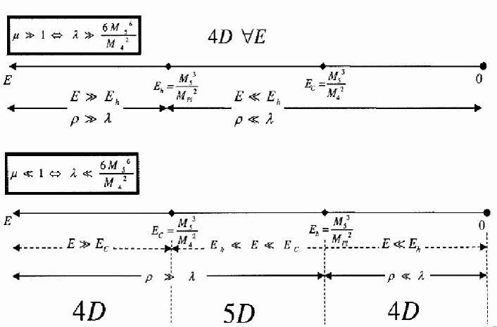
Figure 1: The cosmological evolution of a brane-universe with induced gravity.

In the high energy limit therefore, if $E\gg M^{3}_{5}/M^{2}_{4}$ we have corrections to the four-dimensional Friedmann equation, due to induced gravity, given by

$$H^{2}=\frac{\kappa^{2}_{4}\rho}{3}\Big{(}1+\epsilon\frac{2\sqrt{3}}{\kappa_{4}r_{c}\rho^{1/2}}\Big{)},$$ (32)

and if $M^{3}_{5}/M^{2}_{Pl}\ll E\ll M^{3}_{5}/M^{2}_{4}$ we have corrections to the five-dimensional Friedmann equation of the Randall-Sundrum type

$$H^{2}=\kappa^{4}_{5}\frac{\rho^{2}}{36}\Big{(}1+2\frac{\lambda}{\rho}\Big{)}.$$ (33)

In the next section, we will apply the slow-roll approximation of the inflationary scenario, to the two high energy corrections of the Friedmann equation given by (32) and (33).

3 Inflationary dynamics on the brane

We will assume that the inflationary dynamics is parametrized by a scalar field $\phi$ with a self-interaction potential $V(\phi)$, which is confined on the brane and dominates the energy momentum tensor $T_{\mu\nu}$ on the brane. Then it satisfies the Klein-Gordon equation

$$\ddot{\phi}+3H\dot{\phi}+V^{\prime}(\phi)=0,$$ (34)

since $\nabla^{\mu}T_{\mu\nu}=0$ on the brane. This is equivalent to the continuity equation $\dot{\rho}+3H\rho(1+w)=0$, where we have assume an equation of state $p=w\rho$, with $\rho$ and p given by

$$\rho = \frac{1}{2}\dot{\phi}^{2}+V(\phi),$$ (35)

$$p = \frac{1}{2}\dot{\phi}^{2}-V(\phi).$$ (36)

We are interested on the range of parameter space where inflation potential dominates the brane tension and assume the slow-roll approximation, $\dot{\phi}^{2}\ll V$ and $|\ddot{\phi}|\ll H|\phi|$, and therefore $\rho\approx V$. These assumptions can be justified on the grounds that as we showed in the previous section, induced gravity introduces corrections to the Friedmann equation.

The inflationary parameters $\varepsilon=-\dot{H}/H^{2}$ and $\eta=V^{\prime\prime}/3H^{2}$ with the use of (8), (9) and (11) become

$$\varepsilon = \mu\Big{(}\frac{1}{2\kappa^{2}_{Pl}}\frac{V^{\prime 2}}{V^{2}}\Big{)}\Big{[}\frac{1+\epsilon\,\,2\sqrt{3}\Big{(}A^{2}+4\kappa_{4}^{2}r_{c}^{2}V\Big{)}^{-1/2}}{\Big{(}1+\frac{6}{\kappa^{2}_{4}r^{2}_{c}V}+\frac{\lambda}{V}+\epsilon\,\frac{\sqrt{3}}{\kappa_{4}^{2}r_{c}^{2}V}\Big{(}A^{2}+4\kappa_{4}^{2}r_{c}^{2}V\Big{)}^{1/2}\Big{)}^{2}}\Big{]},$$ (37)

$$\eta = \mu\Big{(}\frac{1}{\kappa^{2}_{Pl}}\frac{V^{\prime\prime}}{V}\Big{)}\Big{[}\frac{1}{1+\frac{6}{\kappa^{2}_{4}r^{2}_{c}V}+\frac{\lambda}{V}+\epsilon\,\frac{\sqrt{3}}{\kappa_{4}^{2}r_{c}^{2}V}\Big{(}A^{2}+4\kappa_{4}^{2}r_{c}^{2}V\Big{)}^{1/2}}\Big{]},$$ (38)

where $A^{2}=(4\kappa^{2}_{4}r^{2}_{c}\lambda+12-2\Lambda_{5}r^{2}_{c})$ and $\mu=\kappa^{2}_{Pl}/\kappa^{2}_{4}$ as it will be discussed later. The term in the curved brackets corresponds to the GR inflationary parameter $\varepsilon$. Hence we can see that for the cosmological evolution with $\mu\ll 1$ induced gravity effects ease for a given potential the condition for slow-roll inflation which is $max\{\varepsilon,|\eta|\}\ll 1$. The number of e-folds during inflation is given by $N=\int^{t_{f}}_{t_{i}}Hdt$ which in the slow-roll approximation using (8) becomes

$$N = -\kappa^{2}_{4}\int^{\phi_{f}}_{\phi_{i}}\frac{V}{V^{\prime}}d\phi-\kappa^{2}_{4}\int^{\phi_{f}}_{\phi_{i}}\frac{1}{V^{\prime}}\Big{(}\lambda+\frac{6}{\kappa_{4}^{2}r_{c}^{2}}\Big{)}d\phi$$ (39)

$$- \epsilon\frac{\sqrt{3}}{r^{2}_{c}}\int^{\phi_{f}}_{\phi_{i}}\frac{1}{V^{\prime}}\Big{(}4\kappa_{4}^{2}r_{c}^{2}V+A^{2}\Big{)}^{1/2}d\phi,$$

where $\phi_{i}$ and $\phi_{f}$ are the values of the inflaton field at the beginning and at the end of inflation. The scalar perturbations in the slow-roll approximation are given by

$$A^{2}_{s}=\frac{1}{\mu^{3}}\Big{(}\frac{\kappa^{6}_{Pl}}{75\pi^{2}}\frac{V^{3}}{V^{\prime 2}}\Big{)}\Big{[}1+\frac{6}{\kappa^{2}_{4}r^{2}_{c}V}+\frac{\lambda}{V}+\epsilon\,\frac{\sqrt{3}}{\kappa_{4}^{2}r_{c}^{2}V}\Big{(}A^{2}+4\kappa_{4}^{2}r_{c}^{2}V\Big{)}^{1/2}\Big{]}^{3}.$$ (40)

We cannot treat the inflationary parameters $\epsilon$ and $\eta$ of (37) and (38) and also equations (39) and (40) analytically due to their complexity. We will analyse instead the inflationary dynamics which arises from the Friedmann equations (32) and (33).

We start first with the Friedmann equation (32). The condition for inflation is

$$\frac{\ddot{a}}{a}=H^{2}+\dot{H}=\frac{\kappa^{2}_{4}}{3}\Big{(}V\Big{(}1+\epsilon\frac{2\sqrt{3}}{\kappa_{4}r_{c}V^{1/2}}\Big{)}-\dot{\phi}^{2}\Big{(}1+\epsilon\frac{\sqrt{3}/2}{\kappa_{4}r_{c}V^{1/2}}\Big{)}\Big{)}>0,$$ (41)

which reduces to

$$\dot{\phi}^{2}\Big{(}1+\epsilon\frac{\sqrt{3}/2}{\kappa_{4}r_{c}V^{1/2}}\Big{)}<V\Big{(}1+\epsilon\frac{2\sqrt{3}}{\kappa_{4}r_{c}V^{1/2}}\Big{)}.$$ (42)

The above condition (42) coincides with the GR condition for inflation when $\kappa_{4}r_{c}V^{1/2}\gg 1$.

Using (32) the slow-roll parameters become

$$\varepsilon = \mu\Big{(}\frac{1}{2\kappa^{2}_{Pl}}\frac{V^{\prime 2}}{V^{2}}\Big{)}\Big{(}1-\epsilon\frac{3\sqrt{3}}{\kappa_{4}r_{c}V^{1/2}}\Big{)},$$ (43)

$$\eta = \mu\Big{(}\frac{1}{\kappa^{2}_{Pl}}\frac{V^{\prime\prime}}{V}\Big{)}\Big{(}1-\epsilon\frac{2\sqrt{3}}{\kappa_{4}r_{c}V^{1/2}}\Big{)}.$$ (44)

Similarly, the number of e-folds during inflation and the scalar perturbations become

$$N = -\frac{\kappa^{2}_{Pl}}{\mu}\int^{\phi_{f}}_{\phi_{i}}\frac{V}{V^{\prime}}\Big{(}1+\epsilon\frac{2\sqrt{3}}{\kappa_{4}r_{c}V^{1/2}}\Big{)}d\phi,$$ (45)

$$A^{2}_{s} = \frac{1}{\mu^{3}}\Big{(}\frac{\kappa^{6}_{Pl}}{75\pi^{2}}\frac{V^{3}}{V^{\prime 2}}\Big{)}\Big{(}1+\epsilon\frac{6\sqrt{3}}{\kappa_{4}r_{c}V^{1/2}}\Big{)}.$$ (46)

Equations (43)-(46) are representing high energy corrections to the general relativity (GR) corresponding quantities in the slow-roll approximation, and coincide with them in the limit $r_{c}\rightarrow\infty$.

Considering a quadratic potential $V=V_{0}\phi^{2}$, in the GR limit $r_{c}\rightarrow\infty$, the spectral index of the scalar perturbation spectrum is independent of $V_{0}$ and it is given by $n_{s}=1+2\eta-6\varepsilon=1-8/\kappa^{2}_{4}\phi^{2}$. Assuming $\phi_{f}\sim 10^{-1}\phi_{i}$, from equations (45) and (46) the values of $V_{0}$ and $\phi_{i}$ can be calculated. Using the COBE normalization for the scalar perturbations $A^{2}_{s}=4\times 10^{-10}$, and for the number of e-folds $N=55$, we find $V_{0}=3.46\times 10^{27}\,(GeV)^{2}$ and $\phi_{i}=1.79\times 10^{20}\,GeV$, while for $N=70$ the numbers are $V_{0}=2.15\times 10^{27}\,(GeV)^{2}$ and $\phi_{i}=2.02\times 10^{20}\,GeV$ respectively. These values of $V_{0}$ correspond to an inflaton mass of $\sim 10^{13}\,GeV$, and the values of the inflaton field are larger than $3M_{4}$. The spectral index of the scalar perturbation spectrum for $N=55$ is $n_{s}=0.9640$, while for $N=70$ we get a larger value of $n_{s}=0.9716$. This is known as the chaotic inflationary scenario [26], and it was criticised for its super-Planckian field values. The problem with the super-Planckian field values is that one expects non-renormalizable quantum corrections to completely dominate the potential, destroying the flatness of the potential required for inflation. This is known as the $\eta$-problem [27].

Coming back to the induced gravity corrections, equation (45) for a quadratic potential becomes

$$N=\frac{\kappa^{2}_{4}\phi^{2}}{4}(1-c^{2})+\epsilon\sqrt{3}\frac{\kappa_{4}\phi}{r_{c}V^{1/2}_{0}}(1-c),$$ (47)

where $\phi=\phi_{i}$ and $c=\phi_{f}/\phi_{i}$. From this equation, the crossover scale can be calculated,

$$r_{c}=\epsilon\frac{\sqrt{3}\kappa_{4}\phi(1-c)}{V_{0}^{1/2}}\Big{(}\frac{4}{4N-\kappa^{2}_{4}\phi^{2}(1-c^{2})}\Big{)}.$$ (48)

To obtain a positive five-dimensional mass $M_{5}$, considering also the GR value of $c\sim 10^{-1}$, equation (48) gives the following conditions for the square of the inflaton field

$$\epsilon = +1,\,\,\ \phi^{2}<\frac{4N}{\kappa^{2}_{4}(1-c^{2})},$$ (49)

$$\epsilon = -1,\,\,\ \phi^{2}>\frac{4N}{\kappa^{2}_{4}(1-c^{2})}.$$ (50)

The spectral index $n_{s}=1+2\eta-6\varepsilon$ using (43) and (44) becomes

$$n_{s}=1-\frac{4}{\kappa^{2}_{4}\phi^{2}}\Big{(}2-\epsilon\frac{7\sqrt{3}}{\kappa_{4}r_{c}\sqrt{V_{0}}\phi}\Big{)}.$$ (51)

Substituting (48) into (51) we can express the inflaton field as a function of the spectral index

$$\phi_{\pm}^{2}=\frac{1}{2\kappa^{2}_{4}(1-n_{s})}\Big{(}(15+7c)\pm\Big{(}\frac{(15+7c)^{2}-112N(1-n_{s})}{(1-c)}\Big{)}^{1/2}\Big{)}.$$ (52)

The inflaton field is well defined if

$$n_{s}>1-\frac{(15+7c)^{2}(1-c)}{112N}.$$ (53)

From this equation, using also (49) and (50) which are the positivity conditions of the crossover scale, we find that the crossover scale is always negative for the solution ($\epsilon=-1,\,\ \phi_{-}$), for the solution ($\epsilon=+1,\,\ \phi_{-}$) is always positive and there is a lower bound for the spectral index given by (53), while for the other solutions we find the following lower or upper bounds for the spectral index $n_{S}$

$$\epsilon=+1,\quad\phi_{+},\quad n_{s} <1-\frac{(15+7c)^{2}(1-c)}{112N},$$ (54)

$$\epsilon=-1,\quad\phi_{+},\quad n_{s} >1-\frac{2(1-c^{2})}{N}.$$ (55)

For $c=10^{-1}$ and for the number of e-folds $N=55$ and $N=70$, the critical value of the spectral index is $n_{s}=0.9640$ and $n_{s}=0.9717$ respectively. Therefore, for the solution having ($\epsilon=+1,\,\ \phi_{+}$) we do not expect any improvement of the value of the spectral index from its GR limit.

Using the COBE normalization for the scalar perturbations $A^{2}_{s}=4\times 10^{-10}$, equation (46), with the use of (48), can give $V_{0}$ as a function of $\phi$

$$V_{0}=\frac{3\pi^{2}(1-c)}{125\times 10^{5}\kappa^{4}_{4}\phi^{2}\Big{(}12N-\kappa^{2}_{4}\phi^{2}(1-c)(1+3c)\Big{)}}.$$ (56)

Demanding a positive $V_{0}$ we get further constraints for the spectral index for the $\phi_{+}$ solution

$$\epsilon=\pm 1,\,\,\ \phi_{+},\,\,\,n_{s}<1-\frac{19(1-c)(1+3c)}{18N},$$ (57)

while for the $\phi_{-}$ it is always positive. For $c=10^{-1}$ and for the number of e-folds $N=55$ and $N=70$, the critical value of the spectral index for these constraints is $n_{s}=0.9775$ and $n_{s}=0.9824$ respectively. Therefore, for the allowed solutions from the positivity constraints, solution ($\epsilon=+1,\,\ \phi_{-}$) has a lower bound of the spectral index but no upper one, while for the solution ($\epsilon=-1,\,\ \phi_{+}$) from (55) and (57) the spectral index is limited to $0.9640<n_{s}<0.9775$ for the number of e-folds $N=55$, and to $0.9717<n_{s}<0.9824$ for the number of e-folds $N=70$.

We can verify these results if we substitute the inflaton field (52) into (56). Then, Fig. 2 shows the variation of the spectral index for various values of $V_{0}$, after having substituting the $\phi_{+}$ solution into (56). There is an upper bound of $n_{s}$ in agreement with (57). In Fig. 3 we plot the variation of the spectral index for the $\phi_{-}$ solution. According to positivity constraints there is no upper bound for the spectral index. Finally, for various values of $V_{0}$ the inflaton field can be calculated and from the crossover scale (48), the five-dimensional mass $M_{5}$ can be specified.

Coming now to the five-dimensional corrections, the Friedmann equation (33) can be written as

$$H^{2}=\mu\frac{\kappa^{2}_{4}\rho}{3}\Big{(}1+\frac{\rho}{2\lambda}\Big{)}.$$ (58)

The $\mu$ parameter which appears in front of $\kappa^{2}_{4}$ also appears in the low energy limit of the Friedmann equation. In order to recover the four dimensional Newton’s constant of early cosmology we have to define

$$\mu\kappa^{2}_{4}=\kappa^{2}_{Pl}.$$ (59)

Performing the same analysis of the inflationary dynamics as before, with the Newton’s constant appearing in (58) identified with the standard four-dimensional Newton’s constant using (59), we find for $N=55$ the spectral index $n_{s}=0.9548$, while for $N=70$ the spectral index becomes $n_{s}=0.9644$ which are the Randall-Sundrum values of the spectral index [28]. The redefinition (59) has important consequences in the early universe. Because $\mu$ is a small number, it gives $G_{4}>G_{Pl}$ which makes gravity stronger [22] in the high energy limit [29].

Figure 2: $V_{0}$ versus $n_{s}$ for the solution $\phi_{+}$ and for the number of e-folds $N=55$ and $N=70$ respectively.

Figure 3: $V_{0}$ versus $n_{s}$ for the solution $\phi_{-}$ and for the number of e-folds $N=55$ and $N=70$ respectively.

4 Chaotic braneworld models with induced gravity

In this section we will search for realistic chaotic inflationary models of induced gravity describing the early evolution. As showed in Fig. 1, for $\lambda\gg 6M_{5}^{6}/M^{2}_{4}$ we have a four-dimensional cosmological evolution for all energies, while if $\lambda\ll 6M_{5}^{6}/M^{2}_{4}$ a four-dimensional evolution is followed by a five-dimensional at high energies. The five-dimensional mass $M_{5}$ in all cases considered in Sec. III, is of the order $\sim 10^{17}\,\,GeV$. Hence, the first case of $\lambda\gg 6M_{5}^{6}/M^{2}_{4}$ is excluded, because we probe a high energy regime where quantum gravity corrections become important.

We studied in Sec. II the cosmological evolution of models with AdS or Minkowski bulk by setting the effective cosmological constant or the five-dimensional cosmological constant equal to zero respectively. In both cases for $\lambda\ll 6M_{5}^{6}/M^{2}_{4}$, and at energies $E\gg M_{5}^{3}/M^{2}_{4}$ the cosmological evolution is described by the Friedmann equation (32). For $\rho\gg\lambda$ and in the energy regime $M^{3}_{5}/M^{2}_{Pl}\ll E\ll M^{3}_{5}/M^{2}_{4}$ the Friedmann equation is given by (33). In the case of an AdS bulk and for $\epsilon=+1$ the brane tension is negative. In general, we expect a negative brane tension to give at late times a negative Newton’s constant.

This is the case in the simplest one-brane Randall-Sundrum model. In this model, the effective gravitational constant in the late time cosmology is identified with the Newton’s constant and a simple relation between the brane tension $\lambda$ the five-dimensional mass $M_{5}$ and the $G_{Pl}$ results. The situation in induced gravity is more subtle. In [25] it was shown that in late time cosmological evolution and without any fine-tuning, the effective gravitational constant is a complicated function of the parameters, and it is changing in time. In our case for the fine-tuning (11) and the approximations we used in Sec. II, in the late time cosmology the Newton’s constant is fixed by relation (59).

Negative tension branes appear quite naturally as endpoints of spacetime in higher than four dimensions. For example they may appear in non-oriented string theories as orientifold planes [30]. In Randall-Sundrum model their presence provides a solution to the hierarchy problem [3] and it appears that they are needed to any realization of geometrical hierarchy in string theories [31]. However, the presence of negative tension branes signals an instability in the bulk-brane system [32]. What really happens is that tachyonic modes are generated via tensor perturbations of the spacetime and bound to the negative tension brane much like the graviton zero-mode to the positive tension brane.

There are various ways to stabilize an unstable bulk-brane system. One way is to introduce a scalar field in the bulk which has self-interaction potentials at the branes. This is the way one can stabilise the two-brane Randall-Sundrum model [33]. Another way is to add an effective cosmological constant. This corresponds to a system rolling down a potential hill towards a different vacuum of the theory. Actually the reason why we find a negative brane tension is that we have put the effective cosmological constant equal to zero in the first place. Finally, one can introduce additional terms in the action in such a way as to drive the system to a stable vacuum.

In the last section we showed that the two solutions ($\epsilon=+1,~{}\phi_{-}$) and ($\epsilon=-1,~{}\phi_{+}$) improve the GR value of the spectral index. However, the solution ($\epsilon=+1,~{}\phi_{-}$) gives the unexpected result of an unbounded from the above spectral index as it is shown in Fig. 3. This is happening because for this solution the inflation never ends. Inflation ends when the slow-roll parameter $\varepsilon=1$. Substituting a quadratic potential $V=V_{0}\phi^{2}$ into (43) we get

$$\varepsilon=\frac{2}{\kappa^{2}_{4}\phi^{2}_{f}}\Big{(}1-\epsilon\frac{3\sqrt{3}}{\kappa_{4}r_{c}\sqrt{V_{0}}\phi_{f}}\Big{)}.$$ (60)

For the solution ($\epsilon=+1,~{}\phi_{-}$) using the GR value $\phi_{f}=10^{-1}\phi_{i}$ we find that the condition at the end of the inflation $\varepsilon=1$ is not satisfied. This is happening because of the negative sign of the second term in (60).

For $E\gg M_{5}^{3}/M^{2}_{4}$ we are left with the solution ($\epsilon=-1,\phi_{+}$). This solution can have positive brane tension for both AdS and Minkowski bulk, well defined energy scales and it gives a spectral index closer to the observations. If we take the GR value of $V_{0}=3.46\times 10^{27}\,(GeV)^{2}$ for the number $N=55$ of e-folds, for $\mu=0.01$ the value of the inflaton field is $2.85\times 10^{18}\,GeV$. The five-dimensional mass is $M_{5}=1.24\times 10^{16}\,GeV$ and it is less than the Planck mass. Therefore we see, that here we do not have the standard problem of the chaotic inflation. The value of the inflaton field is less than the Planck scale, larger however than the five-dimensional mass, and hence we do not expect to have uncontrollable quantum gravity corrections. The reason is that gravity becomes stronger in early cosmological evolution bringing down the value of the inflaton field, as can be seen in (59). The spectral index is $n_{s}=0.9775$ better than the GR value of $n_{s}=0.9640$. If we take $N=70$ for the number of e-folds than the spectral index becomes $n_{s}=0.9824$. In this chaotic inflationary model of the induced gravity the initial value of the potential is not fixed as in the GR limit. The maximum value it can take is $V_{0}^{1/2}=m_{\phi}=10^{-5}M_{P}$ which for $M_{P}=1.2\times 10^{19}\,GeV$ is $V_{0}=1.44\times 10^{28}\,(GeV)^{2}$. Then, with this value of $V_{0}$ the inflaton field and the five-dimensional mass change slightly, so does the spectral index which has already reached its maximum allowed value.

For an energy regime where $M^{3}_{5}/M^{2}_{Pl}\ll E\ll M^{3}_{5}/M^{2}_{4}$ the cosmological evolution is governed by (58). In general this Friedmann equation is giving a different cosmological evolution than the Randall-Sundrum model. However, in the high energy limit $\rho\gg\lambda$, considering the induced gravity as correction to the Randall-Sundrum model, we fix the Newton’s constant from (59) and then we recover the known Randall-Sundrum model results. It is remarkable that the same result applies also to a Minkowski bulk, as this was noticed in [12] in the case of $\Lambda_{5}=0$ and $\lambda=0$.

5 Conclusions

We studied the early time cosmological evolution of a braneworld model with induced gravity when the brane tension and the bulk cosmological constant is included. For $E\gg M_{5}^{3}/M^{2}_{4}$ the evolution is four-dimensional and the Friedmann equation is the standard Friedmann equation of GR supplemented with correction terms due to induced gravity. For $M^{3}_{5}/M^{2}_{Pl}\ll E\ll M^{3}_{5}/M^{2}_{4}$ the evolution is five-dimensional and the Friedmann equation is of the Randall-Sundrum type. In late times and at energies $E\ll M_{5}^{3}/M^{2}_{4}$ the evolution is four-dimensional and the Friedmann equation is the standard Friedmann equation of GR.

We applied the slow-roll inflationary formalism to this model and investigated chaotic inflationary scenarios with AdS or Minkowski bulk. In the induced gravity phase of $E\gg M_{5}^{3}/M^{2}_{4}$, we found better agreement with the recent observations. The spectral index of the scalar perturbation spectrum is $n_{s}=0.9775$ for the number of e-folds $N=55$, while it becomes $n_{s}=0.9824$, for $N=70$. In the five-dimensional phase we recover the Rundall-Sundrum model with the known results of the spectral index of the scalar perturbation spectrum.

An important issue is whether the spectrum of tensor perturbations is altered in the presence of induced gravity, and also what is the relation between the scalar and tensor perturbations. The calculation of tensor perturbations is more involved than the corresponding calculations in the Rundall-Sundrum model [34]. Up to now it is not known what is the spectrum of tensor perturbations in braneworls with induced gravity.

This work can be extended to a braneword cosmological model where both corrections are included in the five-dimensional action: a four-dimensional scalar curvature from induced gravity on the brane, and a five-dimensional Gauss-Bonnet curvature term. In [21] it was shown, that the combined effect of induced gravity and the Gauss-Bonnet term, is to smooth out the initial singularity that is encountered in the individual theories. The resulted model may improve further the value of the spectral index of the scalar perturbation spectrum. It may also help to stabilize the bulk-brane system in the case of a negative tension brane.

Note added: The paper [35] recently appeared which studies the slow-roll inflationary dynamics in the five-dimensional RS sector of the induced gravity model.

Acknowlegements

We thank K. Dimopoulos, G. Kofinas, R. Maartens and D. Wands for valuable discussions and comments. Work supported by the Greek Education Ministry research program ”Hraklitos”.

References

- [1] D. N. Spergel et al., Astrophys. J. Suppl. 148, 175 (2003), astro-ph/0302209.
- [2] A. H. Guth, Phys. Rev. D23, 347 (1981); A. Albrecht and P. J. Steinhardt, Phys. Rev. Lett. 48, 1220 (1982); A. D. Linde, Phys. Lett. 108B, 389 (1982); A. D. Linde, Phys. Lett. 129B, 177 (1983); J. M. Baardeen, P. J. Steinhardt and M. S. Turner, Phys. Rev. D28, 679 (1983).
- [3] L. Randall and R. Sundrum, Phys. Rev. Lett. 83, 3370 (1999), hep-th/9905221; Phys. Rev. Lett. 83, 4690 (1999), hep-th/9906064.
- [4] P. Binétruy, C. Deffayet, U. Ellwanger and D. Langlois, Phys. Lett. 77B, 285 (2000), hep-th/9910219.
- [5] C. Csaki, M. Graesser, C. Kolda and J. Terning, Phys. Lett. 462B, 34 (1999), hep-ph/9906513; J. Cline, C. Grojean and G. Servant, Phys. Rev. Lett. 83, 4245 (1999), hep-ph/9906523.
- [6] R. Maartens, D. Wands, B. Bassett and I. Heard, Phys. Rev. D62, 041301 (2000), hep-ph/9912464.
- [7] S. Tsujikawa and A. R. Liddle, astro-ph/0312162.
- [8] H. Collins and B. Holdom, Phys. Rev. D62, 105009 (2000), hep-ph/0003173.
- [9] G. Dvali, G. Gabadadze and M. Porati, Phys. Lett. 485B, 208 (2000), hep-th/0005016; G. Dvali and G. Gabadadze, Phys. Rev. D63, 065007 (2001), hep-th/0008054.
- [10] D. Lovelock, J. Math. Phys. 12, 498 (1971).
- [11] Y. Shtanov, hep-th/0005193; S. Nojiri and S.D. Odintsov, JHEP 07, 049, (2000) hep-th/0006232; N.J. Kim, H.W. Lee and Y.S. Myung, Phys. Lett. 504B, 323 (2001), hep-th/0101091; C. Deffayet, G. Dvali and G. Gabadadze, Phys. Rev. D65, 044023 (2002), astro-ph/0105068; C. Deffayet, S.J. Landau, J. Raux, M. Zaldarriaga and P. Astier, Phys. Rev. D66, 024019 (2002), astro-ph/0201164.
- [12] C. Deffayet, Phys. Lett. 502B, 199 (2001) hep-th/0010186.
- [13] G. Kofinas, JHEP 08, 034 (2001), hep-th/0108013.
- [14] G. Kofinas, E. Papantonopoulos and I. Pappa, Phys. Rev. D66, 104014 (2002), hep-th/0112019; G. Kofinas, E. Papantonopoulos and V. Zamarias, Phys. Rev. D66, 104028 (2002), hep-th/0208207; A. Lue and G. Starkman, Phys. Rev. D67, 064002 (2003), astro-ph/0212083; G. Dvali, A. Gruzinov and M. Zaldarriaga, Phys. Rev. D68, 024012 (2003), hep-ph/0212069.
- [15] J. E. Kim, B. Kyae and H. M. Lee, Nucl. Phys. B582, 296 (2000), hep-th/0004005; J. E. Kim and H. M. Lee, Nucl. Phys. B602, 346 (2001), hep-th/0010093; S. Nojiri and S. D. Odintsov, Phys. Lett. 493B, 153 (2000), hep-th/0007205; S. Nojiri, S.D. Odintsov and S. Ogushi, Phys. Rev. D65, 023521 (2002), hep-th/0108172; I. P. Neupane, JHEP 09, 040 (2000), hep-th/0008190; I. P. Neupane, Class. Quant. Grav. 19, 5507 (2002), hep-th/0106100; K. A. Meissner and M. Olechowski, Phys. Rev. Lett. 86, 3708 (2001), hep-th/0009122; K. A. Meissner and M. Olechowski, Phys. Rev. D65, 064017 (2002), hep-th/0106203; E. Kiritsis, N. Tetradis and T. Tomaras, JHEP 0108, 012 (2001), hep-th/0106050.
- [16] N. Deruelle and T. Dolezel, Phys. Rev. D62, 103502 (2000), gr-qc/0004021; B. Abdesselam and N. Mohammedi, Phys. Rev. D65, 084018 (2002), hep-th/0110143.
- [17] C. Germani and C. Sopuerta, Phys. Rev. Lett. 88, 231101 (2002), hep-th/0202060.
- [18] C. Charmousis and J. Dufaux, Class. Quantum Grav. 19, 4671 (2002), hep-th/0202107.
- [19] I. Low and A. Zee, Nucl. Phys. B585, 395 (2000), hep-th/0004124; J.E. Lidsey, S. Nojiri and S. Odintsov, JHEP 06, 026 (2002), hep-th/0202198; P. Binetruy, C. Charmousis, S.C. Davis and J-F. Dufaux, Phys. Lett. B544, 183 (2002), hep-th/0206089; J.P. Gregory and A. Padilla, hep-th/0304250; N. Deruelle and M. Sasaki, gr-qc/0306032; C. Barcelo, C. Germani and C.F. Sopuerta, gr-qc/0306072; G. Calcagni, hep-ph/0402126.
- [20] J.E. Lidsey and N.J. Nunes, Phys. Rev. D67, 103510 (2003), astro-ph/0303168.
- [21] G. Kofinas, R. Maartens and E. Papantonopoulos, JHEP, 0310, 066 (2003), hep-th/0307138.
- [22] E. Kiritsis, N. Tetradis and T.N. Tomaras, JHEP 03, 019 (2002), hep-th/0202037.
- [23] V. Sahni and Y. Shtanov, Int. J. Mod. Phys. 11, 1, (2002) gr-qc/0205111 and JCAP 0311 014 2003, astro-ph/0202346; U. Alam and V. Sahni, astro-ph/0209443.
- [24] B. Gumjudpai, gr-qc/0308046.
- [25] K. Maeda, S. Mizuno and T. Torii, Phys. Rev. D68, 024033 (2003), gr-qc/0303039.
- [26] A. D. Linde, Phys. Lett. 129B, 177 (1983).
- [27] D. H. Lyth and A. Riotto, Phys. Rep. 314, 1 (1999), hep-ph/9807278; M. C. Bento and O. Bertolami, Phys. Rev. D65 063513 (2002), astro-ph/0111273; M. C. Bento, O. Bertolami, A. A. Sen, Phys. Rev. D67 023504 (2003), gr-qc/0204046.
- [28] A. R. Liddle and A. J. Smith, astro-ph/0307017.
- [29] We thank Roy Maartens and David Wands for pointed out to us this point.
- [30] J. Polchinski and Y. Cai, Nucl. Phys. B296, 91 (1988); J. Polchinski Phys. Rev. Lett. 75, 4724 (1995), hep-th/9510017.
- [31] S. B. Giddings, S. Kachru and J. Polchinski, Phys. Rev. D66, 106006 (2002), hep-th/0105097.
- [32] C. Charmousis and J.-F. Dufaux, hep-th/0311267.
- [33] W. D. Goldberger and M. B. Wise, Phys. Rev. Lett. 83, 4922 (1999), hep-ph/9907447; O. DeWolfe, D. Z. Freedman, S.S. Gubser and A. Karch, Phys. Rev. D62, 046008 (2000), hep-th/9909134.
- [34] D. Langlois, R. Maartens and D. Wands, Phys. Lett. 489B, 259 (2000).
- [35] H. Zhang and R-G. Cai, hep-th/0403234.