SIMPLICIAL AND ASYMPTOTICAL ASPECTS OF THE HOLOGRAPHIC PRINCIPLE

Se i fatti e la teoria non concordano, cambia i fatti

(Albert Einstein)

Preface

This thesis has been submitted on 12-02-2004 in partial satisfaction of the requirements for the degree Dottore in Ricerca in Fisica in the Department of Nuclear and Theoretical Physics (Pavia University).

The evaluation commetee:

Professor Alberto Rimini

Professor Pietro Menotti

Professor Michele Caselle

Contents

1. 1 Introduction
   1. 1.1 The covariant entropy conjecture
   2. 1.2 Holography and asymptotic symmetries
   3. 1.3 "Intrinsic" holography
   4. 1.4 Outline of the thesis
2. 2 Ribbon graphs and Random Regge Triangulations
   1. 2.1 Triangulated surfaces and Polytopes
      1. 2.1.1 Curvature assignments and divisors.
      2. 2.1.2 Conical Regge polytopes.
      3. 2.1.3 Hyperbolic cusps and cylindrical ends.
   2. 2.2 Ribbon graphs on Regge Polytopes
      1. 2.2.1 The space of 1-skeletons of Regge polytopes.
      2. 2.2.2 Orbifold labelling and dynamical triangulations.
      3. 2.2.3 The ribbon graph parametrization of the moduli space
   3. 2.3 Punctured Riemann surfaces and Regge polytopes.
      1. 2.3.1 A Parametrization of the conical geometry.
3. 3 The WZW model on Random Regge Triangulations
   1. 3.1 The WZW model on a Regge polytope
      1. 3.1.1 Polytopes and the WZW model with boundaries
   2. 3.2 The Quantum Amplitudes at k=1
      1. 3.2.1 The Quantum Amplitudes for the cylindrical ends
      2. 3.2.2 The Ribbon graph insertion operators
      3. 3.2.3 The partition function.
4. 4 Holography and asymptotically flat space-times
   1. 4.1 Emergence of the BMS group in asymptotically flat spacetimes
      1. 4.1.1 BMS as asymptotic symmetry group
      2. 4.1.2 Penrose derivation of the BMS group
      3. 4.1.3 BMS subgroups and angular momentum
   2. 4.2 Bulk entropy and boundary symmetries
      1. 4.2.1 Bulk entropy and BMS boundary symmetries
      2. 4.2.2 Difficulties in reconstructing spacetime and comparison with the AdS case
   3. 4.3 Representations of the BMS group
   4. 4.4 Wave equations
      1. 4.4.1 Wave equations for the BMS group
      2. 4.4.2 Generalizations of the BMS group and possible extensions of the results
   5. 4.5 Implications for the holographic mapping
      1. 4.5.1 Identifying boundary degrees of freedom
      2. 4.5.2 Similarities with ’t Hooft S-matrix Ansatz for black holes
      3. 4.5.3 Remarks on the construction of a S-matrix
5. 5 Conclusion
6. A Induced representations…
   1. A.1 BMS representations in Hilbert topology
   2. A.2 BMS representations in nuclear topology
7. B Wave equations in fiber bundle approach

Chapter 1 Introduction

The history of physics has been characterized by the formulation of leading principles that can describe the structure of different systems and provide the skeleton of all theories. The equivalence principle and the axioms of quantum mechanics are the main examples in this direction. The first is at the basis of general relativity which describes gravity and the macroscopic world whereas the latter gives us the rules to study microscopic systems.

The last fifty years have been characterized by numerous attempts to give a unified description able to combine quantum mechanics with gravity. In this spirit, in the seventies, Hawking studied the propagation of a scalar field in a black hole geometry ultimately discovering that these objects emit a thermal radiation [1]. Furthermore Bekenstein [2] was able to recognize that it is possible to associate to a black hole an entropy

$$S=\frac{A}{4G}+c,$$ (1.1)

where $A$ is the area of the event horizon and $c$ is a constant which is assumed to be bounded. Moreover if we consider a space-time geometry $M$ with a black hole inside, the global system has to obey to a generalized second law of thermodynamics which states

$$\delta S_{T}>0,$$

where $S_{T}$ is the sum of (1.1) and of the entropy of the matter evolving outside the event horizion.

Together with this result, the most striking consequence of the evaporation of a black hole has been derived still by Hawking who recognized that this effect implies a very profound question about the consistency of the usual quantum mechanical operations in a gravitational system [3]. To understand this statement let us consider an asymptotically flat space-time $M$ with a black hole $B$ and a scalar field $\phi$ propagating from $\Im^{-}$ to $\Im^{+}$. The entire evoultion of $\phi$ can be thought as a scattering process where $B$ plays the role of an intermediate state. Assuming that during this event no energy is lost and every conservation law is satisfied then the ordinary rules of quantum mechanics grant us that, if $|in>$ is the initial state of the system on $\Im^{-}$, than an observer on $\Im^{+}$ will see a final state

$$|out>=S|in>,$$

where $S$ is a unitary scattering matrix satisfying $S^{\dagger}=S^{-1}$. A more technical way to read this statement is to recognize that the final state of a system evolving from an initial pure quantum state, has to be pure as well. Bearing this in mind and without entering into unnecessary techniqualities, let us consider an initial scalar particle vacuum state $|0_{-}>$ on $\Im^{-}$ which can be expressed as a combination of states with different number of particles entering into the black hole horizon or escaping to $\Im^{+}$ i.e.

$$|0_{-}>=\sum\lambda_{AB}|A_{+}>|B_{H}>,$$

where $|A_{+}>$ is a state at the future infinity whereas $|B_{H}>$ is a state on the horizon. Furthermore any measure of an observable $Q$ at $\Im^{+}$ will lead to expectation values depending only on the states $|A_{+}>$ and thus in ultimate instance on the creation and annihilation operators of the fields at $\Im^{+}$. This implies that

$$<0_{-}|Q|0_{-}>=\sum\rho_{AC}Q_{CA},$$

where $Q_{CA}=<C_{+}|Q|A_{+}>$ and $\rho_{AC}$ is the density matrix describing all observations made on $\Im^{+}$ and for this reason it depends only on the expectation values of polynomials in the creation and annihilation operators on $\Im^{+}$. In short, the analysis in [3] shows that the above matrix is diagonal in a basis of eigenstates of the number operator; thus after a black hole has completely evaporated, the only possible final states for the radiation at $\Im^{+}$ are those with total energy equal to the intial mass of the black hole and all these configurations can be emitted with equal probability. Eventually the whole process leads to a violation of the principles of quantum mechanics where any consistent scattering process that can bring from a pure state to a mixed one is forbidden.
Furthermore the study of a physical system in presence of an extreme gravitational field does not only lead to a contraddiction with quantum mechanics but even with ordinary results of statistical mechanics. A canonical example comes from Susskind [4] who considers a three dimensional lattice of $\frac{1}{2}$ spin-like degrees of freedom whose fundamental spacing is of the order of the Planck length $l_{p}$. Ordinary statistical mechanics tells us that the number of orthogonal quantum states of the system is $N(V)=2^{n}$ where $n$ is the number of sites occupying a certain region of volume $V$. The maximum entropy available to the system is given by the logarithm of the number of degrees of freedom:

$$S(V)=\log N(V)=\frac{V}{l^{3}_{p}}\log 2,$$ (1.2)

showing a proportionality with the volume. This is in sharp contrast with the Beckenstein formula (1.1) since most of the states contributing to the entropy have an energy far bigger than the one needed for the system to collapse into a black hole and moreover the size of such a black hole could be even greater than $V$ itself.

Going a step further with Susskind’s argument we can consider a region $V$ filled with enough matter in order to have an entropy $S$ bigger than the one of a black hole but without enough energy to form it. Throwing inside other matter increases both the entropy and the energy of the system until a gravitational collapse begins leading to a final configuration with $S$ proportional to the area. Thus the whole process violates the generalized second law of thermodynamics since $\delta S<0$.

The above two examples are simply an indication of the apparent contraddiction between general relativity on a side and quantum mechanics and statistical mechanics on the other side. Both the arguments given by Hawking and Susskind are convincing and difficult to circumvent unless a new radical interpretation is given. The counterproposal was given at the beginning of the nineties by G. ’t Hooft [5] who considered a situation similar to the example discussed above. He argued to radically change the way we count degrees of freedom in such systems: in presence of gravity, an observer can only excite the states with an energy less than the one needed to form a black hole. With this prescription in mind let us consider a gas of particles at a finite temperature $T$. The energy of the system is given by the Boltzmann law:

$$E\propto VT^{4},$$

which implies

$$S\propto VT^{3}.$$

Imposing that $E<\frac{R}{2}$ where $R$ is the Schwartzschild radius of the system (thus no gravitational collapse can occur), then the entropy satisfies the bound

$$S\propto A^{\frac{3}{4}}<A,$$

which could be read as the statement that a black hole is the physical system with the highest reachable entropy. The whole hypotesis provides also an elegant solution to Hawking paradox: the information "lost" inside the black hole which is eventually emitted through a thermal radiation can be possibly recovered bearing in mind that, since the entropy is a measure of the degrees of freedom accessible to the system, then the Beckenstein bound is only another way to say that all the datas inside the black hole can be encoded on the event horizon with a density not exceeding $\rho_{P}$, i.e. on a lattice with the Planck length $l_{P}$ as the characteristic one, one bit of information per lattice site. In such a way there is no more need to break the laws of quantum mechanics in presence of an extreme gravitational field.

Moreover the above concept can be pushed a step further and it can be generalized to the statement that all the information living in a D-dimensional manifold $M$ can be encoded in an hypersurface of codimension $1$ (usually but not necessarly the boundary $\partial M$) with a density of states not exceeding $\rho_{P}$. Thus the main consequence of this idea is that the usual way of counting degrees of freedom in a quantum field theory with a cut-off is highly redundant in a system where gravity is switched on. In this situation if we try to excite more than $\frac{A}{4}$ degrees of freedom, we are taking into account a number of states whose energy leads to the formation of a black hole and thus in ultimate instance they are not accessible. This is the key idea behind ’t Hooft holographic principle.

Since its formulation in 1993 one the main task of modern physics has been to associate to the holographic principle a consistent theory in the same way as general relativity is the natural son of the equivalence principle. Unfortunately up to now there is no such a candidate theory and the main successes in this direction have been only limited to a certain class of systems. We are going now to briefly review them.

1.1 The covariant entropy conjecture

In ultimate analysis the holographic principle represents a new interpretation of the deep physical significance of the Beckenstein bound. Thus a natural step in order to further motivate ’t Hooft conjecture outside the black hole horizon is to look for an entropic bound inside a more generic space-time region.

This question was addressed in a series of papers by Bousso [6] [7] who considered a 3-dimensional space-like region $\Sigma$ in arbitrary 4-dimensional manifold such that its boundary $\partial\Sigma$ is space-like as well. From each point in $\partial\Sigma$ it is possible to construct four light rays, two future directed and two past directed. The set of all these light-like conguences forms the so called "light sheets" whose dynamics is governed by the Raychauduri equation

$$\frac{d\theta}{d\lambda}=-\frac{\theta^{2}}{2}+\omega_{ab}\omega^{ab}+\sigma_{ab}\sigma^{ab}+8\pi R_{ab}k^{a}k^{b},$$ (1.3)

where $\theta=\frac{1}{A}\frac{dA}{d\lambda}$, $\omega_{ab}$ is the torsion tensor, and $\sigma_{ab}$ is the shear tensor.
Bousso prescription is to consider all the light-sheets $L$ with a negative expansion and to follow them until the expansion changes sign or they end on a caustic or at the boundary of the geometry. The covariant entropy conjecture states that the entropy inside these regions satisfies the bound

$$S(L)\leq\frac{A}{4},$$ (1.4)

where $A$ is the area of $\partial\Sigma$.
The conjecture can be clearly viewed as a generalization of Beckenstein work and of all other entropy bounds derived in the framework of general relativity (see as an example [8]). Moreover, by its own construction, the relation (1.4) is manifestly invariant under time reversal which is a property that cannot be understood at a level of thermodynamic only and since there is no assumption about the microscopic physics of the underlying system, the most natural way to interpret Bousso result is at a level of degrees of freedom accessible to the system itself. Thus inspired by ’t Hooft work, Bousso formulated a sort of generalized holographic principle [7]:

Bousso holographic principle: Consider a 2-dimensional region $B$ of area $A$ satisfying the covariant entropy conjecture, then the number $N$ of orthonormal states in the Hilbert space $\mathcal{H}$ describing the physics in the bulk region $L$ satisfies the bound

$$N\leq\exp\frac{A}{4},$$

or equivalently the number of degrees of freedom $N_{dof}$ accesible to the system is

$$N_{dof}\leq\frac{A}{4}.$$

This recipe associate to any two dimensional surface two light-like hypersurfaces with a bounded number of degrees of freedoms. Nonetheless this result is clearly limited to a local a priori fixed region of space-time; on the other hand it would be more interesting to know if it is possible to apply Bousso holographic conjecture to an hypersurface able to store informations from the global space-time and not only from a limited portion. The solution works exaclty inverting the previous prescription: starting from a null hypersurface, one should find the geodesic generators with a non negative expansion until the expansion itself changes sign. This procedure, called by Bousso "projection", identifies a two dimensional spatial surface which is called screen. Moreover inside the class of screens, we can identify a certain subclass represented by the surfaces with a vanishing expansion at any point. The latter are referred to as preferred screens since it has been conjectured in [7] that precisely on these surfaces the holographic bound is saturated. In this thesis, we will show that this concept plays a pivotal role in the construction of an holographic correspondence at a level of quantum field theory. In fact, since it is easy to identify a preferred screen in a wide class of space-times, it will be natural to construct explicitly the dual field theory on such submanifold.

Up to now we have given a background independent formulation of the holographic principle and we have given as well the rules for finding those surface where to encode the bulk information with a density not exceeding one bit of information per Planck area. Eventually, in our hands we have a sort of "geometric" (or classical) holography but up to now we have no clue of what sort of theory we should expect on the (preferred) screens. Clearly we cannot find, even a priori, a conventional quantum field theory since the holographic principle is far more different and elusive than simply assigning some inital datas on a Cauchy surface. Moreover it has been pointed out in [9] that the price for protecting quantum mechanics and general relativity from a reciprocal contraddiction could possibly be the loss of locality in the holographic theory. From one side this is not surprising since it is difficult to conceive a local quantum field theory with cut-off without an entropy proportional to the volume. Nonetheless we could still avert the loss of locality of the theory by introducing an unusual gauge simmetry. Stripping the details of such a formulation let us briefly comment that in this approach, advocated by ’t Hooft and mainly applied to the black hole scenario, we distinguish between "ontological states" growing in number as the volume of the system and "equivalence class" of states growing instead as the area and reproducing the Beckenstein bound. This proposal, although extremely interesting, is quite difficult to apply in a more general setting and it does not reproduce yet Bousso results. For this reason we shall not discuss such an approach any longer.

So far we have used the holographic principle only within the realm of general relativity and the main result has been only to understand where the bound on the number of degrees of freedom can effectively be implemented; the next natural step is to enter the realm of quantum field theory and try to write a theory where such a principle is manifest. The most natural and straightforward scenario would be to construct such an "holographic theory" on a preferred screen where the bound of one bit of information per Planck area is saturated. In this case we expect a kind of dictionary relating the datas on the screen with those in the bulk and we will refer from now on to this situation as the dual theory. Although it seems very difficult to write such a theory for a generic system, up to now the only successful example of an holographic correspondence at a level of quantum field theory, namely the AdS/CFT correspondence, is indeed a dual theory living on the preferred screen of an asymptotically anti de Sitter space-time.
Nonetheless as pointed out by Bousso in [7], the "dual" approach is in general doomed to failure since one of the peculiar aspect of asymptotically AdS space-times is the space-like nature of its boundary. This implies that the number of degrees of freedom is fixed whereas in presence of a time-like boundary such number should evolve in Lorentzian time. In this case we should talk only of a "holographic theory" where the information stored on the screen does not necessarly saturate the Planck limit and a dictionary relating bulk/boundary datas is elusive at best. In this thesis we will advocate this point of view in a more radical way since we will deal with a class of manifolds, the most notable ones being the asymptotically flat space-times, where the natural choice as a preferred screen, i.e. either the boundary $\Im^{+}$ or $\Im^{-}$, is a null submanifold. Thus by its own nature, in such a case, the screen does not provide a good notion of time evolution and the recognition of the degrees of freedom is difficult since we cannot even talk of an "activation" and a "deactivation" of accessible states as advocated by Bousso for time-like screens. We will show that in this context it is difficult as well to keep track of the concept of locality and it is likely that the holographic theory will be most probably very different from a conventional gauge theory.
The final message that we can read from Bousso conjecture is that it can be very difficult to use the holographic principle to "describe nature" since its realization can be extremely elusive and as far as we understand, it is not manifest either in general relativity or in quantum field theory.

1.2 Holography and asymptotic symmetries

At a quantum level the most notable example of the realization of the holographic principle is the AdS/CFT correspondence [10]. Although it is not the purpose of this thesis to explain the details of such theory [11] [12], let us nonetheless point out some of the peculiar aspects characterizing this correspondence as unique by its own nature.

The original Maldacena’s statement deals with the existence of a complete equivalence between type IIB superstring theory in the bulk of $AdS_{5}\otimes S_{5}$ and maximally supersymmetric $3+1$ dimensional $SU(N)$ SYM theory (thus conformally invariant) living on the boundary of the AdS space-time. This correspondence can be geometrically read as a relation between a string theory invariant under $SO(2,d-1)$, the symmetry group of the $AdS_{d}$ space time and a quantum field theory living on $\partial AdS_{d}$ and invariant under the asymptotic symmetry group of the bulk space-time. Moreover, although the gauge/gravity correspondence has been originally introduced in the maximally symmetric background, Maldacena ideas can be generalized to any asymptotically anti-de Sitter background by means of an holographic renormalization group; this technique allows to compute correlation functions of the dual fields only through near boundary computations which rely only upon the asymptotic structure [13]. In this way the original AdS/CFT recipe that associates to every bulk field $\Phi$ a gauge invariant boundary operator $\mathcal{O}_{\Phi}$ is still valid and the boundary values of the bulk fields are identified with sources that couple to dual operators; eventually the on-shell bulk partition function is identified with the generating function of the (bulk) qunatum field theory correlation functions:

$$Z_{sugra}[\Phi_{(0)}]=\int\limits_{\Phi\sim\Phi_{(0)}}[d\Phi]e^{-S[\Phi]}=<\exp(-\int\limits_{\partial AAdS}\Phi_{(0)}\mathcal{O})>_{QFT},$$

where $<,>$ represents the Feynmann quantum field theory expectation value and $\partial AAdS$ is the boundary of an asymptotically anti de Sitter manifold. Following the details of the foundational work of Henneaux and Teitelbom [14] it is clear that the case of negative cosmological constant is quite peculiar; first of all the nature of the boundary itself is extremely unique since, as mentioned before, it is a space-like submanifold which in the spirit of Bousso conjecture represents a preferred screen. As an example let us consider the AdS_d space-time which is topologically equivalent to $\Re\times S^{d-1}$ and can be described through the metric

$$ds^{2}=R^{2}\left[-\frac{1+r^{2}}{1-r^{2}}dt^{2}+\frac{4}{(1-r^{2})^{2}}\left(dr^{2}+r^{2}d\Omega_{d-2}^{2}\right)\right],$$

where $R$ is the curvature radius. Slicing with hypersurfaces of constant time, the boundary is a $2-$sphere (thus a space-like submanifold) at $r=1$ with a divergent area; in the spirit of Bousso’s bound, we can consider the past directed radial light-rays starting from $r=0$ at a certain fixed time. They emanate from a caustic (i.e. $\theta=+\infty$ in (1.3)) and they form a light cone with a spherical boundary which grows in time until it reaches the boundary $r=1$ where it is easy to check that $\theta\to 0$ which, in the language of [7], implies that the AdS boundary is a preferred screen. At a quantum level, instead, the dual theory is invariant under the conformal group ; this enables us to read the bulk/boundary correspondence as a relation between the infrared sectors in $AdS_{d}$ and the ultraviolets sector in $\partial AdS_{d}$ which is a remarkable feature since it has allowed [15] to show explicitly that on the boundary the number of degrees of freedom is bounded by a bit of information per Planck area which is a necessary characteristic of any holographic theory.

A natural question raising from these considerations is whether and to what extent it is possible to follow the road settled by Maldacena in a different background. The work done in (asymptotically) dS space [16], is often based upon analytic continuation from AdS solutions and thus the results so far are of no use in asymptotically flat space-times since the transition of the value of physical relevant quantities from non zero cosmological constant to $\Lambda=0$ is non smooth. Thus, in the $\Lambda=0$ framework what happens is quite different from the AdS case; at a geometric level and in the spirit of finding an holographic theory we notice that in the class of asymptotically flat space-times the notion of preferred screen does not apparently differ from the AdS scenario. Taking as leading example Minkowski space-time, the boundaries $\Im^{\pm}$ are topologically equivalent to $\Re\times S^{d-2}$; in absence of a black hole it is easy to show [7] that the value of $\theta$ goes to $0$ as we approach the boundary. Nonetheless it is imperative to remark that, as soon as a gravitational collapse occur, $\Im^{+}$ does not represent any more a screen since, as we can see drawing the Penrose diagram, part of the information coming from $\Im^{-}$ falls into the black-hole which means, from an holographic point of view, that the datas are stored on the apparent horizon. Nonetheless the past boundary $\Im^{-}$ can always been seen as a preferred screen but this should not mislead us in concluding that the situation is identical to the one experienced in the Maldacena conjecture. In fact, as we shall see in greater details in chapter 4, in asymptotically flat space-times there is a finer relation than in asymptotically AdS manifolds between the asymptotic symmetry group and the background metric. In the $\Lambda=0$ scenario, the group of asymptotic isometries contains not only the Poincaré group which is the bulk symmetry group but also angle-dependent translations which ultimately lead to an infinite dimensional Lie group (the BMS group) [17]. Leaving the details of its derivation to the forthcoming chapters, suffice to say that the BMS group is the semidirect product of the Lorentz group with the set of class $C^{\infty}$ maps from the sphere $S^{d-2}$ to the real numbers and, moreover, it admits a unique four dimensional normal subgroup which is isomorphic to the translation subgroup. A tempting conclusion would be to mod out the non Poincaré part of the BMS group by adding some suitable (but unnatural) boundary conditions but, as we will show, this is impossible whenever the background metric is not stationary. The latter is an unwanted restriction since there is no reason why it should exist a different description of a potential holographic theory in presence of a time dependent or a non time dependent manifold.

From the above remarks, it follows that there is a further significant difference between asymptotically AdS and asymptotically flat space-times. In the first case the preferred screen is a space-like submanifold and the group of asymptotic isometries is a universal structure which ultimately does not depend on the choice of the background metric; on the opposite, in the $\Lambda=0$ scenario, applying Bousso conjecture, it comes natural to store the holographic datas on a null hypersurface whose symmetry group, the Bondi-Metzner-Sachs group, can be reduced in static backgrounds to the Poincaré subgroup. In the spirit of an holographic correspondence, this is a characteristic very difficult to take into account since at first sight it leads us to conclude that in an asymptotically flat background, the bulk/boundary correspondence depends partially upon the chosen metric and at a geometric level it is not a universal feature. Thus, in the spirit of a "universal" gauge/gravity correspondence, we suggest not to distinguish between time and non time-dependent backgrounds and to try to construct the bulk/boundary relation starting from the full BMS group. For this reason we will not start constructing the dual theory as in AdS in the maximally symmetric background (i.e. Minkowski space-time) but we will address the problem in the most general framework.

A further striking difference between the asymptotically AdS and flat scenario comes from the quantum theory. As mentioned before in the AdS/CFT correspondence (and partially in the dS/CFT scenario) the boundary theory is a conformal field theory living on a spacelike manifold; thus we have been able to explicitly derive both the particle spectrum and the correlators for the boundary theory in any asymptotically AdS background and eventually these results led us to discover new insights on the dynamic of the string theory living in the bulk. On the opposite in asymptotically flat space-times the situation is almost reversed since in an holographic scenario we face a boundary theory living on the $\Im^{+}$ or on $\Im^{-}$ which are null submanifolds. This implies that the underlying metric is degenerate and the usual techniques fail since at present there is no direct way to write either a classical or a quantum field theory living on $\Im^{\pm}$. Moreover the spectrum of a BMS field theory is unknown and candidate wave equations are not available. This prevents us to compare, as it has been done in AdS, the Poincaré (bulk) with the BMS (boundary) spectrum in order to understand some feature of the holographic correspondence and write a sort of bulk/boundary dictionary. Nonetheless although we face a great number of odds trying to construct the dual theory, in this thesis we advocate that a line of research looking for an holgraphic theory in asymptotically flat space-times through the BMS group is far more reliable than most of the alternatives proposed until now since most of them deal with the large $R$ limit of the AdS scenario without taking into account the non smooth transition of physical observables between non vanishing and vanishing cosmological constant. Moreover in the above approach the peculiar nature of the asymptotic symmetry group of asymptotically flat space-times is not taken into account and for this reason the geometric difference between stationary and non stationary background, which is non existent in the AdS scenario, is always hidden.
Thus, in this thesis, our first step will be to look at BMS representation theory following the approach that led Wigner [18] to construct the wave equations for the Poincaré group. Our final purpose will be to derive the spectrum of the candidate dual theory and to compare it with the bulk one; nonetheless we can anticipate that, being the Poincaré group a subgroup of the BMS, the particle spectrum of the asymptotic simmetry group of flat manifolds will be larger and richer compared to the Poincaré spectrum thus leading to the natural conjecture that the boundary theory will contain an unnecessary large number of datas.

1.3 "Intrinsic" holography

The holographic principle has been formulated as a conjecture over the counting of degrees of freedom in a physical system without any reference to a particular theory. Nonetheless the successes of AdS/CFT correspondence led often to think to holography as a gauge/gravity correspondence allowing to describe quantum gravity or a quantum field theory in a curved background through a second field theory without gravity living on the boundary. Such a way of thinking, although not without credit, requires ’t Hooft conjecture only as a necessary condition and not as a sufficient one. In particular an interesting line of research would be to explore whether it is possible to strengthen the above remark looking for an holographic correspondence outside the realm of Maldacena example.

Bearing in mind such idea, the most natural candidate in this direction is a $2+1$ space-time; in this framework it has been known since the late eighties [19] that three dimensional gravity (euclidean and non) with non vanishing cosmological constant can be formulated as a Chern-Simons theory. More in detail on a manifold with empty boundary $M$ the action for this system is

$$S=k\int\limits_{M}d^{3}x[A\wedge dA+\frac{2}{3}A\wedge A\wedge A],$$ (1.5)

where $A$ is a connection for the gauge group $SL(2,\mathbb{C})$. An interesting feature of (1.5) emerges if we consider a manifold $M$ such that $\partial M\neq 0$ since we have to add a boundary term to the above action. Supposing, as an example, that the three dimensional variety can be splitted as $M=\Sigma_{g}\times\Re$ where $\Sigma_{g}$ is a Riemann surface, the variation of (1.5) is

$$\delta S=k\int d^{3}x\epsilon^{\mu\nu\rho}Tr(\delta A_{\mu}F_{\nu\rho})+k\int d^{3}x\partial_{\nu}[\epsilon^{\mu\nu\rho}Tr(A_{\mu}\delta A_{\rho})].$$

This formula implies that we have to implement a boundary condition such that $\int\limits_{\partial M}Tr(A\delta A)=0$; taking for simplicity $\Sigma_{g}$ as a disk and interpreting the real axis as a time direction, the above boundary constraint can be achieved imposing that one of the component of the connection, namely the temporal one $A_{0}$, vanishes. With this condition imposed, the gravitational action becomes:

$$S=-k\int_{D\times\Re}d^{3}x\epsilon^{ij}Tr(A_{i}\dot{A}_{j})+\frac{k}{3}\int_{D\times\Re}d^{3}x\epsilon^{ij}Tr(A_{0}F_{ij}).$$

The component $A_{0}$ acts as a Lagrange multiplier leading to the constraint $F_{ij}=0$ which admits as a solution pure gauge connections i.e.

$$A=g^{-1}dg.$$

Substituting this result in the Chern-Simons action, it becomes

$$S=-k\int\limits_{D\times\Re}d\theta dtTr(g^{-1}\partial_{\theta}gg^{-1}\partial_{0}g)+$$

$$+\frac{k}{3}\int_{D\times\Re}d^{3}x\epsilon^{\mu\nu\rho}Tr(g^{-1}\partial_{\mu}gg^{-1}\partial_{\nu}gg^{-1}\partial_{\rho}g).$$ (1.6)

This is exactly the action of a chiral WZW model and more in general it is possible to demonstrate that, dropping the hypotesis that $\Sigma=D$, the Chern-Simons action still induces a WZW boundary term for any compact surface. Moreover a deeper relation between three dimensional gauge theories and CFT can be realized upon quantization of the Chern-Simons action. Without entering into the technical details [20] [21], we are facing a system which, although at first sight the action (1.5) looks highly non linear, can be quantized through a canonical formalism. Working always for simplicity with $M=\Sigma\times\Re$ and with the gauge choice $A_{0}=0$, the procedure consists first in quantizing (1.5) and then in imposing the constraint that the curvature vanishes, i.e. $\frac{\delta\mathcal{L}}{\delta A_{0}}=\epsilon^{ij}F_{ij}^{a}=0$; this implies that we consider as a phase space the moduli space of flat connections over $\Sigma$, modulo gauge transformations. At a geometric level the above procedure is approximately equivalent to the construction of a suitable Hilbert space $\mathcal{H}_{\Sigma}$ over the Riemann surface $\Sigma$; this operation requires the choice of a complex structure $J$ over $\Sigma$ and $\mathcal{H}^{J}_{\Sigma}$ can be interpreted as a holomorphic vector bundle on the moduli space of Riemann surfaces. Moreover since we also require that $\mathcal{H}^{J}_{\Sigma}$ is indipendent from $J$ and depends only on $\Sigma$, this implies the the vector bundle given by $\mathcal{H}^{J}_{\Sigma}$ has flat connections as we expect in a Chern-Simons gauge theory. The above remarks are important since flat bundles appear also in conformal field theory; if one consider, as an example, a current algebra on a Riemann surface with a generic symmetry group $G$ at level $k$, it is a canonical result that, at genus 0, the Ward identities uniquely determine the correlation functions for the identity operator and its descendants. On the opposite, when the genus is greater than $1$, the space of solution of Ward identities for descendants fields of the operator $\mathbb{I}$ is a vector space often named "space of conformal blocks" which, following Segal construction [22], is exactly identical to the above Hilbert space $\mathcal{H}_{\Sigma}$.
Thus starting from these consideration, we are entitled to claim that there is a one to one correspondence between the space of conformal blocks in 1+1 dimensions and the Hilbert space obtained upon quantization of a Chern-Simons gauge theory in 2+1 dimensions. Furthermore, although these results rigorously apply only to a space-time factorizable as $\Sigma\times\Re$, Moore and Seiberg [23] brought Witten’s analysis a step further conjecturing that all the chiral algebras of any rational conformal field theory arise from the quantization of a 3D Chern-Simons gauge theory for some compact Lie group. This hypotesis is clearly very suggestive; it connects in three dimensions the bulk datas which, at quantum level are encoded in the Hilbert space of the theory, to the space of conformal blocks of the boundary theory that are ultimately related to the correlation functions which basically encode the dynamic of the theory.

Although at this stage it would be tempting at first sight to read the above statement as a sort of hint of an holographic correspondence, it is imperative to remark that this would be at best premature. First of all, even if it would be natural to read the CS/WZW relation as a sort of rephrasing of the $AdS_{3}/CFT_{2}$ correspondence, this point of view is unjustified since there is no way to exclude a priori that the two relations are differents. Moreover in the spirit of a gauge/gravity correspondence it is necessary to find a sort of decoupling regime which allows us to separate the bulk from the boundary dynamics but at present time, this is a feature which has not been discovered yet. Nonetheless, taking into account the deep relation described before between the space of states of a Chern-Simons theory and the space of conformal blocks of a WZW model, we still advocate the existence of a sort of "intrinsic" holographic description of the CS/WZW system. Furthermore we claim that, instead of studying an AdS type correspondence in the continuum, the most natural way to look at the bulk/boundary theory in 2+1 dimensions is through a complete different approach; in fact is known that three dimensional euclidean gravity on a manifold with (or without) boundary is equivalent to a discretized model proposed by Ponzano and Regge [24].

Without entering for now in unnecessary technical details [25], in a discretized scenario a D-dimensional manifold is approximated through a polyhedron whose underlying constituent pieces are a collection of D-simplices glued together along a common D-1 dimensional subsimplex. In this scenario, known also as Regge calculus, the main features are to assign to each edge of the triangulation a length and to consider the curvature as concentrated over simplices of codimension 2 known also as hinges or bones; starting from this simple assumption it is possible to give a discretized analogue of Einstein action:

$$S_{E}=\sum\limits_{bones}\epsilon_{i}\mid\sigma_{i}\mid,$$

where $\mid\sigma_{i}\mid$ represents the volume of the i-th flat simplex of codimension 2 and $\epsilon_{i}$ is the so called deficit angle which is equal to the difference between $2\pi$ and the dihedral angles between the faces of the simplices meeting at the hinge.

In the approach proposed by Ponzano and Regge, instead, the recipe is a little bit different: even if we deal with a three dimensional triangulated manifold with the curvature concentrated over one dimensional bones, we label each edge of the simplices with an element $j_{i}$ of the group $SU(2)$ which is ultimately related to the length through the relation $l_{i}=j_{i}\hbar+\frac{1}{2}$. Moreover, starting from the recombinatorial theory of angular momentum, this construction also lead us to naturally associate to each face of a triangle a Wigner $3jm$ symbol and to each tetrahedra a Wigner $6j$ symbol. Starting from these assumptions, the main purpose in [24] was to study the asymptotic formula for the 6j symbol in a sort of semiclassical limit where the assignement $j_{i}$ is diverging, $\hbar\to 0$ but the product $j_{i}\hbar$ (thus in ultimate instance the edge length), is kept fixed. Eventually it was found:

$$\left\{\begin{array}[]{ccc}j_{1}&j_{2}&j_{3}\\ j_{4}&j_{5}&j_{6}\end{array}\right\}\sim\frac{1}{2\pi V}\cos\left(\sum\limits_{i=1}^{6}j_{i}\theta_{i}+\frac{\pi}{4}\right),$$

where $V$ is the volume of the tetrahedron and $\theta_{i}$ is the external dihedral angle at the $i-th$ edge. To connect this formula to quantum gravity let us consider the following topological state sum for a generic three dimensional manifold $M$ with non empty boundary:

$$Z[(M^{3},\partial M^{3})]\,=\,\lim_{L\rightarrow\infty}\>\sum_{\left\{\begin{array}[]{c}(T^{3},\partial T^{3})\\ J,j,m\leq L\end{array}\right\}}Z[(T^{3},\partial T^{3})\rightarrow(M^{3},\partial M^{3});L],$$

$$Z[(T^{3}(J),\partial T^{3}(j;m))\rightarrow(M^{3},\partial M^{3});L]\equiv Z[(T^{3},\partial T^{3});L]=$$ (1.7)

$$\Lambda(L)^{-N_{0}}\,\prod_{1}^{N_{1}}(-1)^{2J}(2J+1)\,\prod_{1}^{N_{3}}(-1)^{\sum J}\>\ \left\{6j\right\}(J)$$

$$\Lambda(L)^{-n_{0}}\,\prod_{1}^{n_{1}}(-1)^{2j}(2j+1)\,\prod_{1}^{N^{F}_{3}}(-1)^{\sum(J+j)}\>\,\left\{6j\right\}(J,j)$$

$$\prod_{1}^{n_{2}}(-1)^{(\sum m)/2}\>\,\left[3jm\right],$$

where $N_{i}$ represents the number of i-th simplices in the triangulation $T^{3}$, $\left\{6j\right\}$ and $\left[3jm\right]$ are respectively the 6j and 3jm $SU(2)$ symbols and $\Lambda(L)$ is a suitable cutoff. In the limit where $\partial M=0$ the above formula reduces to:

$$Z[M^{3}]=\lim_{L\to\infty}\sum_{\left\{T^{3}(j),j\leq L\right\}}Z[T^{3}(j)\rightarrow M^{3};L]$$

$$Z[T^{3}(j)\rightarrow M^{3};L]=\Lambda(L)^{-N_{0}}\prod\limits_{A=1}^{N_{1}}(-)^{2j_{A}}(2j_{A}+1)\prod\limits_{B=1}^{N_{3}}(-)^{\sum\limits_{p=1}^{6}}\left\{\begin{array}[]{ccc}j_{1}&j_{2}&j_{3}\\ j_{4}&j_{5}&j_{6}\end{array}\right\}.$$ (1.8)

In the semiclassical limit, the state sum becomes

$$Z[T^{3}(j);L]=\Lambda(L)^{-N_{0}}\prod\limits_{A=1}^{N_{1}}(-)^{2j_{A}}(2j_{A}+1)\prod\limits_{B=1}^{N_{3}}\frac{(-)^{\sum\limits_{p=1}^{6}}}{2\pi V}\cos\left(\sum\limits_{i=1}^{6}j_{i}\theta_{i}+\frac{\pi}{4}\right),$$ (1.9)

and by exploiting the relation $\cos\theta=\frac{e^{i\theta}+e^{-i\theta}}{2}$, we can recognize in (1.9) a term which looks like a Feynmann sum over histories i.e.

$$\Lambda(L)^{-N_{0}}\prod\limits_{A=1}^{N_{1}}(-)^{2j_{A}}(2j_{A}+1)\prod\limits_{B=1}^{N_{3}}\exp(i\sum\limits_{edges\;l}j_{l}\epsilon_{l}),$$

where $\epsilon_{l}$ is the deficit angle at the edge $l$. Considering the product over the edge lengths as a sort of discretized measure we can interpret the last term in the above formula as a statistical weight a la Feynmann $e^{iS}$ with a Regge type action $S=\sum j_{l}\epsilon_{l}$.

In an holographic setting the wish is to decouple in (1.7) bulk datas from boundary ones and in order to complete this task, we first need to recognize that, in a fixed triangulation, the bulk pieces are described by the fluctuations of the $SU(2)$ assignements of the thetraedra completely inside the manifold whereas the remaining pieces describe the interaction bulk-boundary and are given by those thetraedra having some component on the boundary. In particular, given a triangulation $T^{3}$, we can always refine it in such a way that each thetraedra sharing with the boundary a certain number of faces, has actually only one face on $\partial T^{3}$; this construction provides us with the so called "standard triangulation". In this framework it is easy to distinguish two types of components contributing to the boundary datas: the previously mentioned thetraedra $\{\sigma_{F}\}$ sharing a face with $\partial T^{3}$ whose number will be denoted $N_{3}^{F}$ and those thetraedra sharing a single edge $\{\sigma_{E}\}$ with $\partial T^{3}$ whose number will be $N_{3}^{E}$. These elements represent the coupling thetraedra. In reality, in the spirit of the holographic scenario, in order to decouple the bulk/boundary datas, we should take a proper limit on some metric variable and this role in the PR model is played by those thetraedra with all the edges in the interior of $T^{3}$ but with a single vertex on $\partial T^{3}$; we shall indicate them as $\{\sigma_{V}\}$ and their number will be running from $1$ to $N_{3}^{V}$.

The decoupling procedure implies that all the boundary component are kept fixed and the assignements of "bulk" edges are all rescaled by the same factor $R$. This clearly provides for each separate component a different asymptotic expression (see [27] and references therein for further details):

• for the thetaedra $\sigma_{F}$ we have:

  $$\{6j\}(\sigma_{F},R)\equiv\left\{\begin{array}[]{ccc}j_{1}&j_{2}&j_{3}\\ J_{1}+R&J_{2}+R&J_{3}+R\end{array}\right\}\>\>\>\begin{array}[]{c}\longrightarrow\\ R\gg 1\end{array}\>$$ (1.14)

  $$\frac{(-1)^{\Phi}}{\sqrt{2R}}\>\left[\begin{array}[]{ccc}j_{1}&j_{2}&j_{3}\\ \mu_{1}&\mu_{2}&\mu_{3}\end{array}\right],$$ (1.17)

  where from now on the capital letters are referred to bulk assignments, the small to boundary assignments and $\Phi=j_{1}+j_{2}+j_{3}+2(J_{1}+J_{2}+J_{3})$,

• for the tetrahedra $\sigma_{E}$ we have:

  $$\{6j\}(\sigma_{E},R)\equiv\left\{\begin{array}[]{ccc}J_{1}+R&j&J_{2}+R\\ J_{3}+R&J_{4}+R&J_{5}+R\end{array}\right\}\>\>\>$$ (1.20)

  $$\begin{array}[]{c}\longrightarrow\\ R\gg 1\end{array}\>\frac{(-1)^{\Psi}}{2R}\,\>d^{j}_{\nu_{2}\nu_{3}}(\theta),$$ (1.23)

  where $\Psi=3J_{1}+j+2(J_{2}+J_{3}+J_{4}+J_{5})+\nu_{1}$ and $\theta$ is the angle between the the edge labelled by $j$ and the quantization axis,

• for the tetrahedra $\sigma_{V}$ we have:

  $$\{6j\}(\sigma_{V},R)\equiv\left\{\begin{array}[]{ccc}J_{1}+R&J_{2}+R&J_{2}+R\\ J_{4}+R&J_{5}+R&J_{6}+R\end{array}\right\}\>\>\>\begin{array}[]{c}\longrightarrow\\ R\gg 1\end{array}$$ (1.28)

  $$\left(12\pi{\cal V}(\sigma_{V})\right)^{-1/2}\;\exp\left\{\;i\left(\;\sum_{\alpha=1}^{6}l_{\alpha}\theta_{\alpha}+\pi/4\right)\right\},$$ (1.29)

  where ${\cal V}(\sigma_{V})$ is the Euclidean volume of the tetrahedron spanned by the six edges $\{l_{\alpha}\}$, $l_{\alpha}=J_{\alpha}+1/2$ and $\theta_{\alpha}$ is the angle between the outward normals to the faces which share $l_{\alpha}$ (these angles can be obviously expressed in terms of the $J$’s).

Eventually the partition function associated with this configuration is

$$Z[(T^{3},\partial T^{3})_{st};R\gg 1;L]\,=$$ (1.30)

$$\Lambda(L)^{-N_{0}}\,\>\prod_{1}^{N_{1}-N_{1}^{*}}(-1)^{2J}(2J+1)\,\prod_{1}^{N_{3}-N_{3}^{E}-N_{3}^{V}}(-1)^{\sum J}\>\ \left\{6j\right\}(J)$$

$$\prod_{1}^{N_{1}^{*}}(-1)^{2R}(2R)\>\>\Lambda(L)^{-n_{0}}\>\>\prod_{1}^{n_{1}}(-1)^{2j}\>(2j+1)$$

$$\prod_{1}^{n_{2}}\;(2R)^{-1/2}\>(-1)^{\sum(J+R)+\sum j+\Phi}(-1)^{(\sum m)/2}\left[3j\mu\right]\left[3jm\right]$$

$$\prod_{1}^{N_{3}^{E}}(2R)^{-1}(-1)^{\sum(J+R)+j+\Psi}\>\>d^{j}_{\nu_{2}\,\nu_{3}}(\theta)$$

$$\prod_{1}^{N_{3}^{V}}\;(2R)^{-3/2}(-1)^{\sum(J+R)}\>\exp\left\{i(\sum_{\alpha=1}^{6}l_{\alpha}\theta_{\alpha}+\pi/4)\right\},$$

where $N_{1}^{*}$ is the number of edges of those bulk thetraedra that are not part of the coupling datas.

The last step in order to completely determine the holographic decoupling is to recognize that the topological union of $\{\sigma_{V}\}\cup\{\sigma_{E}\}\cup\{\sigma_{F}\}$ fills in a thick shell of the order of the decoupling parameter $R$ close to the boundary $\partial T^{3}$; we are thus entitled to introduce the triangulation $\tilde{T}^{3}\doteq\left(IntT^{3}\right)-\{\sigma_{V}\}\cup\{\sigma_{E}\}\cup\{\sigma_{F}\}$ and the fixed 2-dimensional triangulation $\Sigma^{in}(R)$ closing up $\tilde{T}^{3}$. The couple $(\tilde{T}^{3},\Sigma^{in}(R))$ is topologically equivalent to $(T^{3},\partial T^{3})$ and moreover $\Sigma^{in}(R)$ represents a sort of "inner boundary" whose intersection with $\partial T^{3}$ is empty. If we now introduce the set $N_{i}(\Sigma^{in}(R))$ of i-simplices in $\Sigma^{in}(R)$, we can associate to $(\tilde{T}^{3},\Sigma^{in}(R)$, the partition function:

$$Z[({\tilde{T}}^{3},\Sigma^{in}(R));L]\,=$$ (1.31)

$$\Lambda(L)^{-(N_{0}-N_{0}(\Sigma^{in}))}\>\,\prod_{1}^{N_{1}-N^{*}_{1}}\;(-1)^{2J}(2J+1)\,\prod_{1}^{N_{3}}(-1)^{\sum J}\>\ \left\{6j\right\}(J)$$

$$\prod_{1}^{N_{1}(\Sigma^{in})}(-1)^{R}(2R)^{1/2}.$$

In the end, the partition function (1.30) can formally be splitted in three parts:

$$Z=Z_{bulk}\mathcal{P}_{bulk\to\;bound}Z_{hol},$$

where $Z_{bulk}=Z[({\tilde{T}}^{3},\Sigma^{in}(R));L]$, $\mathcal{P}_{bulk\to\;bound}$ is a projection map connecting the inner boundary with $\partial T^{3}$ and finally

$$Z^{hol}\>[\Sigma^{out}\,;L]\,=$$ (1.32)

$$\Lambda(L)^{-n_{0}-N_{0}(\Sigma^{in})}\>\prod_{1}^{n_{1}}(-1)^{2j}\>(2j+1)$$

$$\prod_{1}^{n_{2}}\>(-1)^{\sum J+\sum j+\Phi}\>\,(-1)^{(\sum m)/2}\left[3j\mu\right]\>\,\>\left[3jm\right]$$

$$\prod_{1}^{N_{3}^{E}}(-1)^{\sum J+j+\Psi}\>\>d^{j}_{\nu_{2}\,\nu_{3}}(\theta)$$

$$\prod_{1}^{N_{3}^{V}}\;(-1)^{\sum J}\>\exp\left\{i(\sum_{\alpha=1}^{6}l_{\alpha}\theta_{\alpha}+\pi/4)\right\},$$

represents the functional that has to be associated with the holographic partition function.

The first result which comes from the above decoupling is the non topological origin of (1.32) since it is not invariant under Pachner moves; from one side this does not allow us to easily recognize the nature of the above functional but on the other side this remark is rather encouraging in the spirit of an holographic correspondence. Moreover (1.32) shows a residual dependance from bulk datas and more precisely from the asymptotic beahviour of bulk (gravitational) fluctuations. This is in some sense reminding us the AdS/CFT correspondence where the source terms for the boundary theory couple a boundary operator to the asymptotic beahviour of the bulk fields. A deeper look at (1.32) allow us to give prominence to the presence of a pair of 3jm symbols for each vertex with a Wigner symbol connecting them. From one side, this suggests that the boundary functional could possibly be associated to fat trivalent graph which are ultimately dual to 2-dimensional triangulations. From the other side the presence of 3jm symbols in the boundary partition function encourages us to carry on in the direction of finding a relation between (1.32) and a conformal field theory since it is a standard result from Moore and Seiberg [28] that it exists a sort of dictionary between CFT and group theory. In particular it is known that the Clebsh-Gordan coefficients (thus the 3jm symbols) for a compact Lie group $G$ are in one to one correspondence with the chiral vertex operator of the corresponding $G$-invariant conformal theory. Following this line it is also possible to show that the Racah coefficients are associated with the fusion matrices which in the peculiar case of the $SU(2)$ group are exactly the 6j symbols. Thus, within this scheme, it is natural to interpret the functions of the group elements as physical fields in a corresponding CFT and the product of these functions as the standard operator product expansion. Moreover, considering the deep relation existing between Chern-Simons and WZW models, it is also natural to suppose that the boundary theory associated to the system that we are studying is exactly a sort of discretized version of an SU(2) WZW conformal field theory. It is thus intriguing to pursuit this idea trying to relate (1.32) to a WZW action but unfortunately this line of research cannot be swiftly exploited since at present a coherent and universally accepted definition of a conformal field theory over a triangulated surface is unknown. The reason of such "deficency" can be tracked in the underlying big difference between the two models since the discretized rely upon a combinatorial approach which is difficult to apply in the setting of a conformal field theory that is more analytic in spirit. Nonetheless in this thesis we will show that it is possible to circumvent such problem exploting the above mentioned correspondence between triangulated surfaces and ribbon graphs. Roughly speaking, starting from a standard 2-simplicial complex, we will associate to it a dual graph which is ultimately defined through a collection of vertices and edges connecting them. In this simple geometrical construction, that we will outline more in detail in the next chapter, the underlying surface will be "divided" in a collection of closed two dimensional cells; the main feature of this operation will be the chance to define in each cell a uniformizing complex coordinate and a unique quadratic differential (and as a consequence a metric). This result will allow us to switch from the purely combinatorial approach of the simplicial subsdivision of the Riemann surface to a setting which has the twofold advantage from one side to retain the datas from the purely discretized approach and from the other side to introduce analytic tools which are more suitable if we wish to work in the realm of a conformal field theory. Starting from this basis and keeping in mind the correspondence between group theory and CFT outlined mainly by Moore and Seiberg, in this thesis we will adress the problem of the definition of a conformal field theory on a triangulated polyhedron using the techniques coming from the "graph approach" to the discretized setting; nonetheless, bearing in mind that our ultimate goal is to study the holographic correspondence in the Ponzano-Regge calculus and to gain some insight on the true nature of the boundary functional (1.32), we will specialize our analysis on the definition of a WZW model on a triangulated Riemann surface with the gauge group $SU(2)$. In particular, following the works of Gaberdiel [29], we will be able also to explicitly write the partition function for the subcase of a WZW model with gauge group $SU(2)$ at level 1 and eventually to compare this result with (1.32) showing striking similiraties between both formulas.

1.4 Outline of the thesis

As we have mentioned several times in the previous sections, the main purpose of this thesis is to study different physical systems where the holographic principle appears to be realized in a way completely different from Maldacena approach where "holography" is a synonym of a gauge/gravity correspondence that associate to a field theory in a curved background on a bulk manifold $M$, a gauge theory without gravity living on the boundary of $M$. Bearing this in mind and following the motivations of section 1.3 in the next chapter, we study a two dimensional triangulated surface; the leading line will be to introduce several mathematical tools that we will exploit in chapter 3 in order to introduce a WZW model. In particular as we have outlined in the previous section, the natural approach in this scenario is to switch from a triangulation to its dual graph; thus in section 2.1 we start introducing canonical concepts concerning Regge triangulations and in particular we outline the beautiful Troyanov formulation of the Gauss-Bonnet theorem for triangulated manifolds and its implications. The key concepts of this chapter will be outlined in section 2.2 and 2.3 where we will introduce the barycentric subdivision of a two dimensional triangulation $T$. With this geometric construction we will be able to associate to $T$ a dual trivalent graph $P_{T}$ and we will show how it is possible to parametrize through ribbon graphs the moduli space of Riemann surface; moreover we apply Strebel theory of quadratic differential in the context of triangulated surfaces emphasizing the role of uniformizing complex coordinates. In this section as anticipated before we will move from a purely combinatorial language to a more analytic approach endowing the dual graph with a complex structure that will play a pivotal role in the construction of a conformal field theory. The full extent of this change of "language" will be emphasized in chapter 3 which represents the main core of this thesis together with chapter 4. In particular, starting from a Regge polytope we outline in section 3.1 the construction of a WZW model. Since we always bear in mind that our ultimate goal is to apply our results in the context of Ponzano-Regge calculus, we specialize our results to the group $SU(2)$. Starting from this point we will be able to achieve a twofold result: in section 3.2 we construct the Hilbert space for the theory with $G=SU(2)$ at level 1. In particular, since to each dual cell of the dual polytope, is associated a separate Hilbert space, we explicitly describe how they are related introducing insertion operators associated to the ribbon graph that allow to switch from states from one cell into another. In section 3.3 instead we explicitly construct the partition function for the WZW model with group $SU(2)_{1}$ with the hope to relate the result with (1.32). In the end we find striking similarities between the two formulas but we are not still able to make a full correspondence.

In the fourth chapter, instead, we switch from the study of a discretized system in three dimensions to asymptotically flat space-times. As in the previous chapters, our ultimate goal is to provide new insights in the realization of the holographic principle in this framework. As for the Ponzano-Regge scenario, we study mainly the asymptotic dynamics of the theory whose informations in a flat background are encoded in the asymptotic symmetry group, the Bondi-Metzner-Sachs group. For this reason in section 4.1 we review the derivation and the main features of this group. In particular we emphasize its twofold nature as an asymptotic symmetry group from one side and on the other side as the intrinsic symmetry group of the manifold $\Im$. Starting from this remark and bearing in mind Bousso covariant entropy conjecture, we address in section 4.2 the problem of a geometric reconstrucion of the bulk space-time starting from datas encoded in $\Im$ ultimately finding that, due to high focusing of light rays, a geometric holography is possible only within a restricted class of manifolds, namely the stationary ones. Thus this result forces us to switch our attention to the quantum level in order to implement the holographic principle and the main problem that we face is the absence of a BMS field theory. For this reason our first priority will be to determine BMS wave equations and we will follow a purely group theoretical way; after extensively reviewing in section 4.4 McCarthy theory of representation, we present in section 4.5 our main result which is the construction of BMS wave equations with the a method similar to the one used by Wigner for the Poincaré group. Moreover we will emphasize the asymptotic role of these fields, i.e. they evolve only on $\Im$ and they never propagate in the bulk; this remark will suggest us to pursuit a road similar to ’t Hooft ansatz of introducing an S-matrix in order to describe propagation of informations from $\Im^{+}$ to $\Im^{-}$. Furthermore the structure of the fields equations will allow us to conjecture that any holographic correspondence in asymptotically flat space-times has to show an high degree of non locality.
Finally in the last chapter, after reviewing our main results, we discuss open questions mainly referring to the holographic principle and we present some further relation between our work and different approaches. In the end our aim will be also to briefly discuss some possible future line of research which could have this thesis as a starting point.

The content and the figures available in this thesis have been taken in part from the following papers [30], [31], [32].

Chapter 2 Ribbon graphs and Random Regge Triangulations

The aim of this chapter will be mainly to describe the deep relation existing between random Regge triangulations and trivalent ribbon graphs. We will follow the lines of [34] and [30] even though we will not concentrate on the description of the modular aspects of two dimensional gravity; instead we will emphasize the role of the uniformizing coordinates and of the Strebel theorem as the main tools needed in order to define a conformal field theory over a triangulated Riemann surface. In essence this chapter should be seen as preparatory for an application to the WZW model and for the study of the relation between CS/WZW in a discretized setting.

2.1 Triangulated surfaces and Polytopes

Let $T$ denote a $2$-dimensional simplicial complex with underlying polyhedron $|T|$ and $f$- vector $(N_{0}(T),N_{1}(T),N_{2}(T))$, where $N_{i}(T)\in\mathbb{N}$ is the number of $i$-dimensional sub-simplices $\sigma^{i}$ of $T$. Given a simplex $\sigma$ we denote by $st(\sigma)$, (the star of $\sigma$), the union of all simplices of which $\sigma$ is a face, and by $lk(\sigma)$, (the link of $\sigma$), is the union of all faces $\sigma^{f}$ of the simplices in $st(\sigma)$ such that $\sigma^{f}\cap\sigma=\emptyset$. A Regge triangulation of a $2$ -dimensional PL manifold $M$, (without boundary), is a homeomorphism $|T_{l}|\rightarrow{M}$ where each face of $T$ is geometrically realized by a rectilinear simplex of variable edge-lengths $l(\sigma^{1}(k))$. A dynamical triangulation $|T_{l=a}|\rightarrow{M}$ is a particular case of a Regge PL-manifold realized by rectilinear and equilateral simplices of edge-length $l(\sigma^{1}(k))=a$ (see figure 2.1).

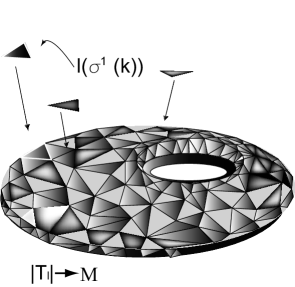
Figure 2.1: A torus triangulated with triangles of variable edge-length.

The metric structure of a Regge triangulation is locally Euclidean everywhere except at the vertices $\sigma^{0}$, (the bones), where the sum of the dihedral angles, $\theta(\sigma^{2})$, of the incident triangles $\sigma^{2}$’s is in excess (negative curvature) or in defect (positive curvature) with respect to the $2\pi$ flatness constraint. The corresponding deficit angle $\varepsilon$ is defined by $\varepsilon=2\pi-\sum_{\sigma^{2}}\theta(\sigma^{2})$, where the summation is extended to all $2$-dimensional simplices incident on the given bone $\sigma^{0}$. If $K_{T}^{0}$ denotes the $(0)$-skeleton of $|T_{l}|\rightarrow{M}$, (i.e., the collection of vertices of the triangulation), then $M\backslash{K_{T}^{0}}$ is a flat Riemannian manifold, and any point in the interior of an $r$- simplex $\sigma^{r}$ has a neighborhood homeomorphic to $B^{r}\times{C}(lk(\sigma^{r}))$, where $B^{r}$ denotes the ball in $\mathbb{R}^{n}$ and ${C}(lk(\sigma^{r}))$ is the cone over the link $lk(\sigma^{r})$, (the product $lk(\sigma^{r})\times[0,1]$ with $lk(\sigma^{r})\times\{1\}$ identified to a point). In particular, let us denote by $C|lk(\sigma^{0}(k))|$ the cone over the link of the vertex $\sigma^{0}(k)$. On any such a disk $C|lk(\sigma^{0}(k))|$ we can introduce a locally uniformizing complex coordinate $\zeta(k)\in\mathbb{C}$ in terms of which we can explicitly write down a conformal conical metric locally characterizing the singular structure of $|T_{l}|\rightarrow M$, viz.,

$$e^{2u}\left|\zeta(k)-\zeta_{k}(\sigma^{0}(k))\right|^{-2\left(\frac{\varepsilon(k)}{2\pi}\right)}\left|d\zeta(k)\right|^{2},$$ (2.1)

where $\varepsilon(k)$ is the corresponding deficit angle, and $u:B^{2}\rightarrow\mathbb{R}$ is a continuous function ($C^{2}$ on $B^{2}-\{\sigma^{0}(k)\}$) such that, for $\zeta(k)\rightarrow\zeta_{k}(\sigma^{0}(k))$, we have $\left|\zeta(k)-\zeta_{k}(\sigma^{0}(k))\right|\frac{\partial u}{\partial\zeta(k)}$, and $\left|\zeta(k)-\zeta_{k}(\sigma^{0}(k))\right|\frac{\partial u}{\partial\overline{\zeta}(k)}$ both $\rightarrow 0$, [35]. Up to the presence of $e^{2u}$, we immediately recognize in such an expression the metric $g_{\theta(k)}$ of a Euclidean cone of total angle $\theta(k)=2\pi-\varepsilon(k)$. The factor $e^{2u}$ allows to move within the conformal class of all metrics possessing the same singular structure of the triangulated surface $|T_{l}|\rightarrow M$. We can profitably shift between the PL and the function theoretic point of view by exploiting standard techniques of complex analysis, and making contact with moduli space theory (see figure 2.2).

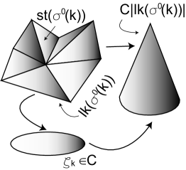
Figure 2.2: The geometric structures around a vertex.

2.1.1 Curvature assignments and divisors.

In the case of dynamical triangulations, the picture simplifies considerably since the deficit angles are generated by the numbers $\#\{\sigma^{2}(h)\bot\sigma^{0}(i)\}$ of triangles incident on the $N_{0}(T)$ vertices, the curvature assignments, $\{q(k)\}_{k=1}^{N_{0}(T)}\in\mathbb{N}^{N_{0}(T)}$,

$$q(i)=\frac{2\pi-\varepsilon(i)}{\arccos(1/2)}.$$ (2.2)

For a regular triangulation we have $q(k)\geq 3$, and since each triangle has $3$ vertices $\sigma^{0}$, the set of integers $\{q(k)\}_{k=1}^{N_{0}(T)}$ is constrained by

$$\sum_{k=1}^{N_{0}}q(k)=3N_{2}=6\left[1-\frac{\chi(M)}{N_{0}(T)}\right]N_{0}(T),$$ (2.3)

where $\chi(M)$ denotes the Euler-Poincaré characteristic of the surface, and where $6\left[1-\frac{\chi(M)}{N_{0}(T)}\right]$, ($\simeq 6$ for $N_{0}(T)>>1$), is the average value of the curvature assignments $\{q(k)\}_{k=1}^{N_{0}}$. More generally we shall consider semi-simplicial complexes for which the constraint $q(k)\geq 3$ is removed. Examples of such configurations are afforded by triangulations with pockets, where two triangles are incident on a vertex, or by triangulations where the star of a vertex may contain just one triangle. We shall refer to such extended configurations as generalized (Regge and dynamical) triangulations.

The singular structure of the metric defined by (2.1) can be naturally summarized in a formal linear combination of the points $\{\sigma^{0}(k)\}$ with coefficients given by the corresponding deficit angles (normalized to $2\pi$), in the real divisor [35]

$$Div(T)\doteq\sum_{k=1}^{N_{0}(T)}\left(-\frac{\varepsilon(k)}{2\pi}\right)\sigma^{0}(k)=\sum_{k=1}^{N_{0}(T)}\left(\frac{\theta(k)}{2\pi}-1\right)\sigma^{0}(k)$$ (2.4)

supported on the set of bones $\{\sigma^{0}(i)\}_{i=1}^{N_{0}(T)}$. Note that the degree of such a divisor, defined by

$$\left|Div(T)\right|\doteq\sum_{k=1}^{N_{0}(T)}\left(\frac{\theta(k)}{2\pi}-1\right)=-\chi(M)$$ (2.5)

is, for dynamical triangulations, a rewriting of the combinatorial constraint (2.3). In such a sense, the pair $(|T_{l=a}|\rightarrow M,Div(T))$, or shortly, $(T,Div(T))$, encodes the datum of the triangulation $|T_{l=a}|\rightarrow M$ and of a corresponding set of curvature assignments $\{q(k)\}$ on the vertices $\{\sigma^{0}(i)\}_{i=1}^{N_{0}(T)}$. The real divisor $\left|Div(T)\right|$ characterizes the Euler class of the pair $(T,Div(T))$ and yields for a corresponding Gauss-Bonnet formula. Explicitly, the Euler number associated with $(T,Div(T))$ is defined, [35], by

$$e(T,Div(T))\doteq\chi(M)+|Div(T)\mathbf{|.}$$ (2.6)

and the Gauss-Bonnet formula reads [35]:

Lemma 1

(Gauss-Bonnet for triangulated surfaces) Let $(T,Div(T))$ be a triangulated surface with divisor

$$Div(T)\doteq\sum_{k=1}^{N_{0}(T)}\left(\frac{\theta(k)}{2\pi}-1\right)\sigma^{0}(k),$$ (2.7)

associated with the vertices $\{\sigma^{0}(k)\}_{k=1}^{N_{0}(T)}$. Let $ds^{2}$ be the conformal metric (2.1) representing the divisor $Div(T)$ . Then

$$\frac{1}{2\pi}\int_{M}KdA=e(T,Div(T)),$$ (2.8)

where $K$ and $dA$ respectively are the curvature and the area element corresponding to the local metric $ds_{(k)}^{2}.$

Note that such a theorem holds for any singular Riemann surface $\Sigma$ described by a divisor $Div(\Sigma)$ and not just for triangulated surfaces [35]. Since for a Regge (dynamical) triangulation, we have $e(T_{a},Div(T))=0$, the Gauss-Bonnet formula implies

$$\frac{1}{2\pi}\int_{M}KdA=0.$$ (2.9)

Thus, a triangulation $|T_{l}|\rightarrow M$ naturally carries a conformally flat structure. Clearly this is a rather obvious result, (since the metric in $M-\{\sigma^{0}(i)\}_{i=1}^{N_{0}(T)}$ is flat). However, it admits a not-trivial converse (recently proved by M. Troyanov, but, in a sense, going back to E. Picard) [35], [36]:

Theorem 2

(Troyanov-Picard) Let $(\left(M,\mathcal{C}_{sg}\right),Div)$ be a singular Riemann surface with a divisor such that $e(M,Div)=0$. Then there exists on $M$ a unique (up to homothety) conformally flat metric representing the divisor $Div$.

2.1.2 Conical Regge polytopes.

Let us consider the (first) barycentric subdivision of $T$. The closed stars, in such a subdivision, of the vertices of the original triangulation $T_{l}$ form a collection of $2$-cells $\{\rho^{2}(i)\}_{i=1}^{N_{0}(T)}$ characterizing the conical Regge polytope $|P_{T_{l}}|\rightarrow{M}$ (and its rigid equilateral specialization $|P_{T_{a}}|\rightarrow{M}$) barycentrically dual to $|T_{l}|\rightarrow{M}$. If $(\lambda(k),\chi(k))$ denote polar coordinates (based at $\sigma^{0}(k)$) of a point $p\in\rho^{2}(k)$, then $\rho^{2}(k)$ is geometrically realized as the space

$$\left.\left\{(\lambda(k),\chi(k))\ :\lambda(k)\geq 0;\chi(k)\in\mathbb{R}/(2\pi-\varepsilon(k))\mathbb{Z}\right\}\right/(0,\chi(k))\sim(0,\chi^{\prime}(k))$$ (2.10)

endowed with the metric

$$d\lambda(k)^{2}+\lambda(k)^{2}d\chi(k)^{2},$$ (2.11)

as it can be seen in figure 2.3.

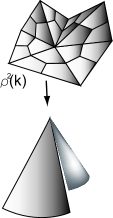
Figure 2.3: The conical geometry of the baricentrically dual polytope.

In other words, here we are not considering a rectilinear presentation of the dual cell complex $P$ (where the PL-polytope is realized by flat polygonal $2$-cells $\{\rho^{2}(i)\}_{i=1}^{N_{0}(T)}$) but rather a geometrical presentation $|P_{T_{l}}|\rightarrow{M}$ of $P$ where the $2$ -cells $\{\rho^{2}(i)\}_{i=1}^{N_{0}(T)}$ retain the conical geometry induced on the barycentric subdivision by the original metric (2.1) structure of $|T_{l}|\rightarrow{M}$.

2.1.3 Hyperbolic cusps and cylindrical ends.

It is important to stress that whereas a Regge triangulation characterizes a unique (up to automorphisms) singular Euclidean structure, this latter actually allows for a more general type of metric triangulation. The point is that some of the vertices associated with a singular Euclidean structure can be characterized by deficit angles $\varepsilon(k)\rightarrow 2\pi$i.e., $\sum_{\sigma^{2}(k)}\theta(\sigma^{2}(k))=0$. Such a situation corresponds to having the cone $C|lk(\sigma^{0}(k))|$ over the link $lk(\sigma^{0}(k))$ realized by a Euclidean cone of angle $0$. This is a natural limiting case in a Regge triangulation, (think of a vertex where many long and thin triangles are incident), and it is usually discarded as an unwanted pathology. However, there is really nothing pathological about that, since the corresponding $2$-cell $\rho^{2}(k)\in|P_{T_{l}}|\rightarrow{M}$ can be naturally endowed with the conformal Euclidean structure obtained from (2.1) by setting $\frac{\varepsilon(k)}{2\pi}=1$, i.e.

$$e^{2u}\left|\zeta(k)-\zeta_{k}(\sigma^{0}(k))\right|^{-2}\left|d\zeta(k)\right|^{2},$$ (2.12)

which (up to the conformal factor $e^{2u}$) is the flat metric on the half-infinite cylinder $\mathbb{S}^{1}\times\mathbb{R}^{+}$ (a cylindrical end, see figure 2.4).

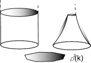
Figure 2.4: The cylindrical and hyperbolic metric over a $\theta\to 0$ degenerating polytopal cell.

Alternatively, one may consider $\rho^{2}(k)$ endowed with the geometry of a hyperbolic cusp, i.e., that of a half-infinite cylinder $\mathbb{S}^{1}\times\mathbb{R}^{+}$ equipped with the hyperbolic metric $\lambda(k)^{-2}(d\lambda(k)^{2}+d\chi(k)^{2})$. The triangles incident on $\sigma^{0}(k)$ are then realized as hyperbolic triangles with the vertex $\sigma^{0}(k)$ located at $\lambda(k)=\infty$ and corresponding angle $\theta_{k}=0$[37]. Since the Poincaré metric on the punctured disk $\{\zeta(k)\in C|\;0<\left|\zeta(k)-\zeta_{k}(\sigma^{0}(k))\right|<1\}$ is

$$\left(\left|\zeta(k)-\zeta_{k}(\sigma^{0}(k))\right|\ln\frac{1}{\left|\zeta(k)-\zeta_{k}(\sigma^{0}(k))\right|}\right)^{-2}\left|d\zeta(k)\right|^{2},$$ (2.13)

one can shift from the Euclidean to the hyperbolic metric by setting

$$e^{2u}=\left(\ln\frac{1}{\left|\zeta(k)-\zeta_{k}(\sigma^{0}(k))\right|}\right)^{-2},$$ (2.14)

and the two points of view are strictly related. At any rate the presence of hyperbolic cusps or cylindrical ends is consistent with a singular Euclidean structure as long as the associated divisor satisfies the topological constraint (2.5), which we can rewrite as

$$\sum_{\{\frac{\varepsilon(k)}{2\pi}\neq 1\}}\left(-\frac{\varepsilon(k)}{2\pi}\right)=2g-2+\#\left\{\sigma^{0}(h)|\;\frac{\varepsilon(h)}{2\pi}=1\right\}.$$ (2.15)

In particular, we can have the limiting case of the singular Euclidean structure associated with a genus $g$ surface triangulated with $N_{0}-1$ hyperbolic vertices $\{\sigma^{0}(k)\}_{k=1}^{N_{0}-1}$ (or, equivalently, with $N_{0}-1$ cylindrical ends) and just one standard conical vertex, $\sigma^{0}(N_{0})$, supporting the deficit angle

$$-\frac{\varepsilon(N_{0})}{2\pi}=2g-2+(N_{0}-1).$$ (2.16)

2.2 Ribbon graphs on Regge Polytopes

The geometrical realization of the $1$-skeleton of the conical Regge polytope $|P_{T_{l}}|\rightarrow{M}$ is a $3$-valent graph

$$\Gamma=(\{\rho^{0}(k)\},\{\rho^{1}(j)\})$$ (2.17)

where the vertex set $\{\rho^{0}(k)\}_{k=1}^{N_{2}(T)}$ is identified with the barycenters of the triangles $\{\sigma^{o}(k)\}_{k=1}^{N_{2}(T)}\in|T_{l}|\rightarrow M$, whereas each edge $\rho^{1}(j)\in\{\rho^{1}(j)\}_{j=1}^{N_{1}(T)}$ is generated by two half-edges $\rho^{1}(j)^{+}$ and $\rho^{1}(j)^{-}$ joined through the barycenters $\{W(h)\}_{h=1}^{N_{1}(T)}$ of the edges $\{\sigma^{1}(h)\}$ belonging to the original triangulation $|T_{l}|\rightarrow M$. If we formally introduce a ghost-vertex of a degree $2$ at each middle point $\{W(h)\}_{h=1}^{N_{1}(T)}$, then the actual graph naturally associated to the $1$-skeleton of $|P_{T_{l}}|\rightarrow{M}$ is the edge-refinement [38] of $\Gamma=(\{\rho^{0}(k)\},\{\rho^{1}(j)\})$, i.e.

$$\Gamma_{ref}=\left(\{\rho^{0}(k)\}\bigsqcup_{h=1}^{N_{1}(T)}\{W(h)\},\{\rho^{1}(j)^{+}\}\bigsqcup_{j=1}^{N_{1}(T)}\{\rho^{1}(j)^{-}\}\right),$$ (2.18)

as it can be seen in figure 2.5.

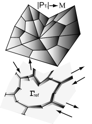
Figure 2.5: The dual polytope around a vertex and it’s edge refinement.

The natural automorphism group $Aut(P_{l})$ of  $|P_{T_{l}}|\rightarrow{M}$, (i.e., the set of bijective maps $\Gamma=(\{\rho^{0}(k)\},\{\rho^{1}(j)\})\rightarrow\widetilde{\Gamma}=(\widetilde{\{\rho^{0}(k)\}},\widetilde{\{\rho^{1}(j)\}}$ preserving the incidence relations defining the graph structure), is the automorphism group of its edge refinement [38], $Aut(P_{l})\doteq Aut(\Gamma_{ref})$. The locally uniformizing complex coordinate $\zeta(k)\in\mathbb{C}$ in terms of which we can explicitly write down the singular Euclidean metric (2.1) around each vertex $\sigma^{0}(k)\in$ $|T_{l}|\rightarrow M$, provides a (counterclockwise) orientation in the $2$-cells of $|P_{T_{l}}|\rightarrow{M}$. Such an orientation gives rise to a cyclic ordering on the set of half-edges $\{\rho^{1}(j)^{\pm}\}_{j=1}^{N_{1}(T)}$ incident on the vertices $\{\rho^{0}(k)\}_{k=1}^{N_{2}(T)}$. According to these remarks, the $1$-skeleton of $|P_{T_{l}}|\rightarrow{M}$ is a ribbon (or fat) graph [25], a graph $\Gamma$ together with a cyclic ordering on the set of half-edges incident to each vertex of $\Gamma$. Conversely, any ribbon graph $\Gamma$ characterizes an oriented surface $M(\Gamma)$ with boundary possessing $\Gamma$ as a spine, (i.e., the inclusion $\Gamma\hookrightarrow M(\Gamma)$ is a homotopy equivalence). In this way (the edge-refinement of) the $1$-skeleton of a generalized conical Regge polytope $|P_{T_{l}}|\rightarrow{M}$ is in a one-to-one correspondence with trivalent metric ribbon graphs. The set of all such trivalent ribbon graph $\Gamma$ with given edge-set $e(\Gamma)$ can be characterized [38], [39] as a space homeomorphic to $\mathbb{R}_{+}^{|e(\Gamma)|}$, ($|e(\Gamma)|$ denoting the number of edges in $e(\Gamma)$), topologized by the standard $\epsilon$-neighborhoods $U_{\epsilon}\subset$ $\mathbb{R}_{+}^{|e(\Gamma)|}$. The automorphism group $Aut(\Gamma)$ acts naturally on such a space via the homomorphism $Aut(\Gamma)\rightarrow\mathfrak{G}_{e(\Gamma)}$, where $\mathfrak{G}_{e(\Gamma)}$ denotes the symmetric group over $|e(\Gamma)|$ elements, and the resulting quotient space $\mathbb{R}_{+}^{|e(\Gamma)|}/Aut(\Gamma)$ is a differentiable orbifold.

2.2.1 The space of 1-skeletons of Regge polytopes.

Let $Aut_{\partial}(P_{l})\subset Aut(P_{l})$, denote the subgroup of ribbon graph automorphisms of the (trivalent) $1$-skeleton $\Gamma$ of $|P_{T_{l}}|\rightarrow{M}$ that preserve the (labeling of the) boundary components of $\Gamma$. Then, the space $K_{1}RP_{g,N_{0}}^{met}$ of $1$-skeletons of conical Regge polytopes $|P_{T_{l}}|\rightarrow{M}$, with $N_{0}(T)$ labelled boundary components, on a surface $M$ of genus $g$ can be defined by [38]

$$K_{1}RP_{g,N_{0}}^{met}=\bigsqcup_{\Gamma\in RGB_{g,N_{0}}}\frac{\mathbb{R}_{+}^{|e(\Gamma)|}}{Aut_{\partial}(P_{l})},$$ (2.19)

where the disjoint union is over the subset of all trivalent ribbon graphs (with labelled boundaries) satisfying the topological stability condition $2-2g-N_{0}(T)<0$, and which are dual to generalized triangulations. It follows, (see [38] theorems 3.3, 3.4, and 3.5), that the set $K_{1}RP_{g,N_{0}}^{met}$ is locally modelled on a stratified space constructed from the components (rational orbicells) $\mathbb{R}_{+}^{|e(\Gamma)|}/Aut_{\partial}(P_{l})$ by means of a (Whitehead) expansion and collapse procedure for ribbon graphs, which amounts to collapsing edges and coalescing vertices, (the Whitehead move in $|P_{T_{l}}|\rightarrow{M}$ is the dual of the familiar flip move [25] for triangulations). Explicitly, if $l(t)=tl$ is the length of an edge $\rho^{1}(j)$ of a ribbon graph $\Gamma_{l(t)}\in$ $K_{1}RP_{g,N_{0}}^{met}$, then, as $t\rightarrow 0$, we get the metric ribbon graph $\widehat{\Gamma}$ which is obtained from $\Gamma_{l(t)}$ by collapsing the edge $\rho^{1}(j)$. By exploiting such construction, we can extend the space $K_{1}RP_{g,N_{0}}^{met}$ to a suitable closure $\overline{K_{1}RP}_{g,N_{0}}^{met}$ [39], (this natural topology on $K_{1}RP_{g,N_{0}}^{met}$ shows that, at least in two-dimensional quantum gravity, the set of Regge triangulations with fixed connectivity does not explore the full configurational space of the theory). The open cells of $K_{1}RP_{g,N_{0}}^{met}$, being associated with trivalent graphs, have dimension provided by the number $N_{1}(T)$ of edges of $|P_{T_{l}}|\rightarrow{M}$, i.e.

$$\dim\left[K_{1}RP_{g,N_{0}}^{met}\right]=N_{1}(T)=3N_{0}(T)+6g-6.$$ (2.20)

There is a natural projection

$$p:K_{1}RP_{g,N_{0}}^{met}\longrightarrow\mathbb{R}_{+}^{N_{0}(T)}$$ (2.21)

$$\Gamma\longmapsto p(\Gamma)=(l_{1},...,l_{N_{0}(T)}),$$

where $(l_{1},...,l_{N_{0}(T)})$ denote the perimeters of the polygonal 2-cells $\{\rho^{2}(j)\}$ of $|P_{T_{l}}|\rightarrow{M}$. With respect to the topology on the space of metric ribbon graphs, the orbifold $K_{1}RP_{g,N_{0}}^{met}$ endowed with such a projection acquires the structure of a cellular bundle. For a given sequence $\{l(\partial(\rho^{2}(k)))\}$, the fiber

$$p^{-1}(\{l(\partial(\rho^{2}(k)))\})=\left\{|P_{T_{l}}|\rightarrow{M}\in K_{1}RP_{g,N_{0}}^{met}:\{l_{k}\}=\{l(\partial(\rho^{2}(k)))\}\right\}$$ (2.22)

is the set of all generalized conical Regge polytopes with the given set of perimeters. If we take into account the $N_{0}(T)$ constraints associated with the perimeters assignments, it follows that the fibers $p^{-1}(\{l(\partial(\rho^{2}(k)))\})$ have dimension provided by

$$\dim\left[p^{-1}(\{l(\partial(\rho^{2}(k)))\}\right]=2N_{0}(T)+6g-6,$$ (2.23)

which again corresponds to the real dimension of the moduli space $\mathfrak{M}_{g},_{N_{0}}$ of $N_{0}$-pointed Riemann surfaces of genus $g$.

2.2.2 Orbifold labelling and dynamical triangulations.

Let us denote by

$$\Omega_{T_{a}}\doteq\frac{\mathbb{R}_{+}^{|e(\Gamma)|}}{Aut_{\partial}(P_{T_{a}})}$$ (2.24)

the rational cell associated with the 1-skeleton of the conical polytope $|P_{T_{a}}|\rightarrow{M}$ dual to a dynamical triangulation $|T_{l=a}|\rightarrow M$. The orbicell (2.24) contains the ribbon graph associated with $|P_{T_{a}}|\rightarrow{M}$ and all (trivalent) metric ribbon graphs $|P_{T_{L}}|\rightarrow{M}$ with the same combinatorial structure of $|P_{T_{a}}|\rightarrow{M}$ but with all possible length assignments $\{l(\rho^{1}(h))\}_{h=1}^{N_{1}(T)}$ associated with the corresponding set of edges $\{\rho^{1}(h)\}_{1}^{N_{1}(T)}$. The orbicell $\Omega_{T_{a}}$ is naturally identified with the convex polytope (of dimension $(2N_{0}(T)+6g-6)$) in $\mathbb{R}_{+}^{N_{1}(T)}$ defined by

$$\left\{\{l(\rho^{1}(j))\}\in\mathbb{R}_{+}^{N_{1}(T)}:\sum_{j=1}^{q(k)}A_{(k)}^{j}(T_{a})l(\rho^{1}(j))\,=\frac{\sqrt{3}}{3}aq(k),\;k=1,...,N_{0}\;\right\},$$ (2.25)

where $A_{(k)}^{j}(T_{a})$ is a $(0,1)$ indicator matrix, depending on the given dynamical triangulation $|T_{l=a}|\rightarrow M$, with $A_{(k)}^{j}(T_{a})=1$ if the edge $\rho^{1}(j)$ belongs to $\partial(\rho^{2}(k))$, and $0$ otherwise, and $\frac{\sqrt{3}}{3}aq(k)$ is the perimeter length $l(\partial(\rho^{2}(k)))$ in terms of the corresponding curvature assignment $q(k)$. Note that $|P_{T_{a}}|\rightarrow{M}$ appears as the barycenter of such a polytope.

Since the cell decomposition (2.19) of the space of trivalent metric ribbon graphs $K_{1}RP_{g,N_{0}}^{met}$ depends only on the combinatorial type of the ribbon graph, we can use the equilateral polytopes $|P_{T_{a}}|\rightarrow{M}$, dual to dynamical triangulations, as the set over which the disjoint union in (2.19) runs. Thus we can write

$$K_{1}RP_{g,N_{0}}^{met}=\bigsqcup_{\mathcal{DT}(N_{0})}\Omega_{T_{a}},$$ (2.26)

where

$$\mathcal{DT}_{g}\left(N_{0}\right)\doteq\left\{|T_{l=a}|\rightarrow M\;:(\sigma^{0}(k))\;k=1,...,N_{0}(T)\right\}$$ (2.27)

denote the set of distinct generalized dynamically triangulated surfaces of genus $g$, with a given set of $N_{0}(T)$ ordered labelled vertices.

Note that, even if the set $\mathcal{DT}_{g}\left(N_{0}\right)$ can be considered (through barycentrical dualization) a well-defined subset of $K_{1}RP_{g,N_{0}}^{met}$, it is not an orbifold over $\mathbb{N}$ [40]. For this latter reason, the analysis of the metric stuctures over (generalized) polytopes requires the use of the full orbicells $\Omega_{T_{a}}$ and we cannot limit our discussion to equilateral polytopes.

2.2.3 The ribbon graph parametrization of the moduli space

We start by recalling that the moduli space $\mathfrak{M}_{g},_{N_{0}}$ of genus $g$ Riemann surfaces with $N_{0}$ punctures is a dense open subset of a natural compactification (Knudsen-Deligne-Mumford ) in a connected, compact complex orbifold denoted by $\overline{\mathfrak{M}}_{g},_{N_{0}}$. This latter is, by definition, the moduli space of stable $N_{0}$-pointed curves of genus $g$, where a stable curve is a compact Riemann surface with at most ordinary double points such that all of its parts are hyperbolic. The closure $\partial\mathfrak{M}_{g},_{N_{0}}$ of $\mathfrak{M}_{g},_{N_{0}}$ in $\overline{\mathfrak{M}}_{g},_{N_{0}}$ consists of stable curves with double points, and gives rise to a stratification decomposing $\overline{\mathfrak{M}}_{g},_{N_{0}}$ into subvarieties. By definition, a stratum of codimension $k$ is the component of $\overline{\mathfrak{M}}_{g},_{N_{0}}$ parametrizing stable curves (of fixed topological type) with $k$ double points.

The complex analytic geometry of the space of conical Regge polytopes which we will discuss in the next section generalizes the well-known bijection (a homeomorphism of orbifolds) between the space of metric ribbon graphs $K_{1}RP_{g,N_{0}}^{met}$ (which forgets the conical geometry) and the moduli space $\mathfrak{M}_{g},_{N_{0}}$ of genus $g$ Riemann surfaces $((M;N_{0}),\mathcal{C})$ with $N_{0}(T)$ punctures [38], [39]. This bijection results in a local parametrization of $\mathfrak{M}_{g},_{N_{0}}$ defined by

$$h:K_{1}RP_{g,N_{0}}^{met}\rightarrow\mathfrak{M}_{g},_{N_{0}}\times{R}_{+}^{N}$$ (2.28)

$$\Gamma\longmapsto[((M;N_{0}),\mathcal{C}),l_{i}]$$

where $(l_{1},...,l_{N_{0}})$ is an ordered n-tuple of positive real numbers and $\Gamma$ is a metric ribbon graphs with $N_{0}(T)$ labelled boundary lengths $\{l_{i}\}$ (see figure 2.6).

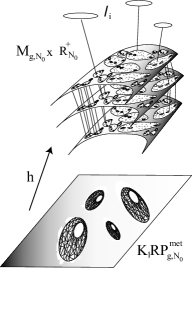
Figure 2.6: The map $h$ associates to each ribbon graph an element of the decorated moduli space $\mathfrak{M}_{g,N_{0}}\times\Re^{+}_{N_{0}}$.

If $\overline{K_{1}RP}_{g,N_{0}}^{met}$ is the closure of $K_{1}RP_{g,N_{0}}^{met}$, then the bijection $h$ extends to $\overline{K_{1}RP}_{g,N_{0}}^{met}\rightarrow\overline{\mathfrak{M}}_{g},_{N_{0}}\times{R}_{+}^{N_{0}}$ in such a way that a ribbon graph $\Gamma\in\overline{RGP}_{g,N_{0}}^{met}$ is mapped in two (stable) surfaces $M_{1}$ and $M_{2}$ with $N_{0}(T)$ punctures if and only if there exists an homeomorphism between $M_{1}$ and $M_{2}$ preserving the (labelling of the) punctures, and is holomorphic on each irreducible component containing one of the punctures.

According to Kontsevich [41], corresponding to each marked polygonal 2-cells $\{\rho^{2}(k)\}$ of $|P_{T_{l}}|\rightarrow{M}$ there is a further (combinatorial) bundle map

$$\mathcal{CL}_{k}\rightarrow K_{1}RP_{g,N_{0}}^{met}$$ (2.29)

whose fiber over $(\Gamma,\rho^{2}(1),...,\rho^{2}(N_{0}))$ is provided by the boundary cycle $\partial\rho^{2}(k)$, (recall that each boundary $\partial\rho^{2}(k)$ comes with a positive orientation).

To any such cycle one associates [39], [41] the corresponding perimeter map $l(\partial(\rho^{2}(k)))=\sum$ $l(\rho^{1}(h_{\alpha}))$ which then appears as defining a natural connection on $\mathcal{CL}_{k}$. The piecewise smooth 2-form defining the curvature of such a connection,

$$\omega_{k}(\Gamma)=\sum_{1\leq h_{\alpha}<h_{\beta}\leq q(k)-1}d\left(\frac{l(\rho^{1}(h_{\alpha}))}{l(\partial\rho^{2}(k))}\right)\wedge d\left(\frac{l(\rho^{1}(h_{\beta}))}{l(\partial\rho^{2}(k))}\right),$$ (2.30)

is invariant under rescaling and cyclic permutations of the $l(\rho^{1}(h_{\mu}))$, and is a combinatorial representative of the Chern class of the line bundle $\mathcal{CL}_{k}$.

It is important to stress that even if ribbon graphs can be thought of as arising from Regge polytopes (with variable connectivity), the morphism (2.28) only involves the ribbon graph structure and the theory can be (and actually is) developed with no reference at all to a particular underlying triangulation. In such a connection, the role of dynamical triangulations has been slightly overemphasized, they simply provide a convenient way of labelling the different combinatorial strata of the mapping (2.28), but, by themselves they do not define a combinatorial parametrization of $\overline{\mathfrak{M}}_{g},_{N_{0}}$ for any finite $N_{0}$. However, it is very useful, at least for the purposes of quantum gravity, to remember the possible genesis of a ribbon graph from an underlying triangulation and be able to exploit the further information coming from the associated conical geometry. Such an information cannot be recovered from the ribbon graph itself (with the notable exception of equilateral ribbon graphs, which can be associated with dynamical triangulations), and must be suitably codified by adding to the boundary lengths $\{l_{i}\}$ of the graph a further decoration. This can be easily done by explicitly connecting Regge polytopes to punctured Riemann surfaces.

2.3 Punctured Riemann surfaces and Regge polytopes.

As suggested by (2.1), the polyhedral metric associated with the vertices $\{\sigma^{0}(i)\}$ of a (generalized) Regge triangulation $|T_{l}|\rightarrow M$, can be conveniently described in terms of complex function theory. We can extend the ribbon graph uniformization of [38] and associate with the polytope $|P_{T_{l}}|\rightarrow{M}$ a complex structure $((M;N_{0}),\mathcal{C})$ (a punctured Riemann surface) which is, in a well-defined sense, dual to the structure (2.1) generated by $|T_{l}|\rightarrow M$. Let $\rho^{2}(k)$ be the generic two-cell $\in|P_{T_{l}}|\rightarrow{M}$ barycentrically dual to the vertex $\sigma^{0}(k)\in|T_{l}|\rightarrow M$. To the generic edge $\rho^{1}(h)$ of $\rho^{2}(k)$ we associate a complex uniformizing coordinate $z(h)$ defined in the strip

$$U_{\rho^{1}(h)}\doteq\{z(h)\in\mathbb{C}\;|\;0<\mathop{\mathrm{R}e}z(h)<l(\rho^{1}(h))\},$$ (2.31)

$l(\rho^{1}(h))$ being the length of the edge considered. The uniformizing coordinate $w(j)$, corresponding to the generic $3$-valent vertex $\rho^{0}(j)\in\rho^{2}(k)$, is defined in the open set

$$U_{\rho^{0}(j)}\doteq\{w(j)\in\mathbb{C}\;|\;|w(j)|<\delta,\;w(j)[\rho^{0}(j)]=0\},$$ (2.32)

where $\delta>0$ is a suitably small constant. Finally, the two-cell $\rho^{2}(k)$ is uniformized in the unit disk

$$U_{\rho^{2}(k)}\doteq\{\zeta(k)\in\mathbb{C}\;|\;|\zeta(k)|<1,\;\zeta(k)[\sigma^{0}(k)]=0\},$$ (2.33)

where $\sigma^{0}(k)$ is the vertex $\in|T_{l}|\rightarrow M$ corresponding to the given two-cell (see figure 2.7).

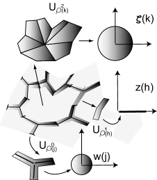
Figure 2.7: The local presentation of uniformizing coordinates.

The various uniformizations $\{w(j),U_{\rho^{0}(j)}\}_{j=1}^{N_{2}(T)}$, $\{z(h),U_{\rho^{1}(h)}\}_{h=1}^{N_{1}(T)}$, and $\{\zeta(k),U_{\rho^{2}(k)}\}_{k=1}^{N_{0}(T)}$ can be coherently glued together by noting that to each edge $\rho^{1}(h)\in$ $\rho^{2}(k)$ we can associate the standard quadratic differential on $U_{\rho^{1}(h)}$ given by

$$\phi(h)|_{\rho^{1}(h)}=dz(h)\otimes dz(h).$$ (2.34)

Such $\phi(h)|_{\rho^{1}(h)}$ can be extended to the remaining local uniformizations $U_{\rho^{0}(j)}$, and $U_{\rho^{2}(k)}$, by exploiting a classic result in Riemann surface theory according to which a quadratic differential $\phi$ has a finite number of zeros $n_{zeros}(\phi)$ with orders $k_{i}$ and a finite number of poles $n_{poles}(\phi)$ of order $s_{i}$ such that

$$\sum_{i=1}^{n_{zero}(\phi)}k_{i}-\sum_{i=1}^{n_{pole}(\phi)}s_{i}=4g-4.$$ (2.35)

In our case we must have $n_{zeros}(\phi)=N_{2}(T)$ with $k_{i}=1$, (corresponding to the fact that the $1$-skeleton of $|P_{l}|\rightarrow M$ is a trivalent graph), and $n_{poles}(\phi)=$ $N_{0}(T)$ with $s_{i}=s\;\forall i$, for a suitable positive integer $s$. According to such remarks (2.35) reduces to

$$N_{2}(T)-sN_{0}(T)=4g-4.$$ (2.36)

From the Euler relation $N_{0}(T)-N_{1}(T)+N_{2}(T)=2-2g$, and $2N_{1}(T)=3N_{2}(T)$ we get $N_{2}(T)-2N_{0}(T)=4g-4$. This is consistent with (2.36) if and only if $s=2$. Thus the extension $\phi$ of $\phi(h)|_{\rho^{1}(h)}$ along the $1$-skeleton of $|P_{l}|\rightarrow M$ must have $N_{2}(T)$ zeros of order $1$ corresponding to the trivalent vertices $\{\rho^{0}(j)\}$ of $|P_{l}|\rightarrow M$ and $N_{0}(T)$ quadratic poles corresponding to the polygonal cells $\{\rho^{2}(k)\}$ of perimeter lengths $\{l(\partial(\rho^{2}(k)))\}$. Around a zero of order one and a pole of order two, every (Jenkins-Strebel [42]) quadratic differential $\phi$ has a canonical local structure which (along with (2.34)) is given by [38][42]

$$(|P_{T_{l}}|\rightarrow{M)\rightarrow}\phi\doteq\left\{\begin{tabular}[]{l}$\phi(h)|_{\rho^{1}(h)}=dz(h)\otimes dz(h),$\\ $\phi(j)|_{\rho^{0}(j)}=\frac{9}{4}w(j)dw(j)\otimes dw(j),$\\ $\phi(k)|_{\rho^{2}(k)}=-\frac{\left[l(\partial(\rho^{2}(k)))\right]^{2}}{4\pi^{2}\zeta^{2}(k)}d\zeta(k)\otimes d\zeta(k),$\end{tabular}\right.$$ (2.37)

where $\{\rho^{0}(j),\rho^{1}(h),\rho^{2}(k)\}$ runs over the set of vertices, edges, and $2$-cells of $|P_{T_{l}}|\rightarrow M$. Since $\phi(h)|_{\rho^{1}(h)}$, $\phi(j)|_{\rho^{0}(j)}$, and $\phi(k)|_{\rho^{2}(k)}$ must be identified on the non-empty pairwise intersections $U_{\rho^{0}(j)}\cap U_{\rho^{1}(h)}$, $U_{\rho^{1}(h)}\cap U_{\rho^{2}(k)}$ we can associate to the polytope $|P_{T_{l}}|\rightarrow{M}$ a complex structure $((M;N_{0}),\mathcal{C})$ by coherently gluing, along the pattern associated with the ribbon graph $\Gamma$, the local uniformizations $\{U_{\rho^{0}(j)}\}_{j=1}^{N_{2}(T)}$, $\{U_{\rho^{1}(h)}\}_{h=1}^{N_{1}(T)}$, and  $\{U_{\rho^{2}(k)}\}_{k=1}^{N_{0}(T)}$. Explicitly, let $\{U_{\rho^{1}(j_{\alpha})}\}$, $\alpha=1,2,3$ be the three generic open strips associated with the three cyclically oriented edges $\{\rho^{1}(j_{\alpha})\}$ incident on the generic vertex $\rho^{0}(j)$. Then the uniformizing coordinates $\{z(j_{\alpha})\}$ are related to $w(j)$ by the transition functions

$$w(j)=e^{2\pi i\frac{\alpha-1}{3}}z(j_{\alpha})^{\frac{2}{3}},\hskip 14.45377pt\hskip 7.22743pt\alpha=1,2,3.$$ (2.38)

Note that in such uniformization the vertices $\{\rho^{0}(j)\}$ do not support conical singularities since each strip $U_{\rho^{1}(j_{\alpha})}$ is mapped by (2.38) into a wedge of angular opening $\frac{2\pi}{3}$. This is consistent with the definition of $|P_{T_{l}}|\rightarrow{M}$ according to which the vertices $\{\rho^{0}(j)\}\in|P_{T_{l}}|\rightarrow{M}$ are the barycenters of the flat $\{\sigma^{2}(j)\}\in|T_{l}|\rightarrow M$. Similarly, if $\{U_{\rho^{1}(k_{\beta})}\}$, $\beta=1,2,...,q(k)$ are the open strips associated with the $q(k)$ (oriented) edges $\{\rho^{1}(k_{\beta})\}$ boundary of the generic polygonal cell $\rho^{2}(k)$, then the transition functions between the corresponding uniformizing coordinate $\zeta(k)$ and the $\{z(k_{\beta})\}$ are given by [38]

$$\zeta(k)=\exp\left(\frac{2\pi i}{l(\partial(\rho^{2}(k)))}\left(\sum_{\beta=1}^{\nu-1}l(\rho^{1}(k_{\beta}))+z(k_{\nu})\right)\right),\hskip 14.45377pt\nu=1,...,q(k),$$ (2.39)

with $\sum_{\beta=1}^{\nu-1}\cdot\doteq 0$, for $\nu=1$.

2.3.1 A Parametrization of the conical geometry.

Note that for any closed curve $c:\mathbb{S}^{1}\rightarrow U_{\rho^{2}(k)}$, homotopic to the boundary of $\overline{U}_{\rho^{2}(k)}$, we get

$$\oint_{c}\sqrt{\phi(k)_{\rho^{2}(k)}}=l(\partial(\rho^{2}(k))).$$ (2.40)

which shows that the geometry associated with $\phi(k)_{\rho^{2}(k)}$ is described by the cylindrical metric canonically associated with a quadratic differential with a second order pole,i.e.

$$|\phi(k)_{\rho^{2}(k)}|=\frac{\left[l(\partial(\rho^{2}(k)))\right]^{2}}{4\pi^{2}|\zeta(k)|^{2}}|d\zeta(k)|^{2}.$$ (2.41)

If we denote by

$$\Delta_{k}^{\ast}\doteq\{\zeta(k)\in\mathbb{C}|\;0<|\zeta(k)|<1\},$$ (2.42)

the punctured disk $\Delta_{k}^{\ast}\subset U_{\rho^{2}(k)}$, then for each given deficit angle $\varepsilon(k)=2\pi-\theta(k)$ we can introduce on each $\Delta_{k}^{\ast}$ the conical metric

$$ds_{(k)}^{2} \doteq \frac{\left[L(k)\right]^{2}}{4\pi^{2}}\left|\zeta(k)\right|^{-2\left(\frac{\varepsilon(k)}{2\pi}\right)}\left|d\zeta(k)\right|^{2}=$$

$$= \left|\zeta(k)\right|^{2\left(\frac{\theta(k)}{2\pi}\right)}|\phi(k)_{\rho^{2}(k)}|.$$

It follows that we can apply the explicit construction [38] of the mapping (2.28) for defining the decorated Riemann surface corresponding to a conical Regge polytope. Then, an obvious adaptation of theorem 4.2 of [38] provides

Proposition 3

Let $\{p_{k}\}_{k=1}^{N_{0}}\in M$ denote the set of punctures corresponding to the decorated vertices $\{\sigma^{0}(k),\frac{\varepsilon(k)}{2\pi}\}_{k=1}^{N_{0}}$ of the triangulation $|T_{l}|\rightarrow M$ and let $\Gamma$ be the ribbon graph associated with the corresponding dual conical polytope $(|P_{T_{l}}|\rightarrow{M)}$, then the map

$$\Upsilon:(|P_{T_{l}}|\rightarrow{M)\longrightarrow}((M;N_{0}),\mathcal{C});\{ds_{(k)}^{2}\})$$ (2.44)

$$\Gamma\longmapsto\bigcup_{\{\rho^{0}(j)\}}^{N_{2}(T)}U_{\rho^{0}(j)}\bigcup_{\{\rho^{1}(h)\}}^{N_{1}(T)}U_{\rho^{1}(h)}\bigcup_{\{\rho^{2}(k)\}}^{N_{0}(T)}(U_{\rho^{2}(k)},ds_{(k)}^{2}),$$

defines the decorated, $N_{0}$-pointed, Riemann surface $((M;N_{0}),\mathcal{C})$ canonically associated with the conical Regge polytope $|P_{T_{l}}|\rightarrow{M}$.

In order to describe the geometry of the uniformization of $((M;N_{0}),\mathcal{C}))$ defined by $\{ds_{(k)}^{2}\}$, let us consider the image in $((M;N_{0}),\mathcal{C}))$ of the generic triangle $\sigma^{2}(h,j,k)\in|T_{l}|\rightarrow M$ of sides $\sigma^{1}(h,j)$, $\sigma^{1}(j,k)$, and $\sigma^{1}(k,h)$. Similarly, let $W(h,j)$, $W(j,k)$, and $W(k,h)$ be the images of the respective barycenters, (see (2.18)). Denote by $\widehat{L}(k)=|W(h,j)\rho^{0}(h,j,k)|$, $\widehat{L}(h)=|W(j,k)\rho^{0}(h,j,k)|$, and $\widehat{L}(j)=|W(k,h)\rho^{0}(h,j,k)|$, the lengths, in the metric $\{ds_{(k)}^{2}\}$, of the half-edges connecting the (image of the) vertex $\rho^{0}(h,j,k)$ of the ribbon graph $\Gamma$ with $W(h,j)$, $W(j,k)$, and $W(k,h)$. Likewise, let us denote by $l(\bullet,\bullet)$ the length of the corresponding side $\sigma^{1}(\bullet,\bullet)$ of the triangle. A direct computation involving the geometry of the medians of $\sigma^{2}(h,j,k)$ provides

$$\begin{tabular}[]{ccc}$\widehat{L}^{2}(j)$&$=$&$\frac{1}{18}l^{2}(j,k)+\frac{1}{18}l^{2}(h,j)-\frac{1}{36}l^{2}(k,h)$\\ $\widehat{L}^{2}(k)$&$=$&$\frac{1}{18}l^{2}(k,h)+\frac{1}{18}l^{2}(j,k)-\frac{1}{36}l^{2}(h,j)$\\ $\widehat{L}^{2}(h)$&$=$&$\frac{1}{18}l^{2}(h,j)+\frac{1}{18}l^{2}(k,h)-\frac{1}{36}l^{2}(j,k)$\\ &&\\ $l^{2}(k,h)$&$=$&$8\widehat{L}^{2}(h)+8\widehat{L}^{2}(k)-4\widehat{L}^{2}(j)$\\ $l^{2}(h,j)$&$=$&$8\widehat{L}^{2}(j)+8\widehat{L}^{2}(h)-4\widehat{L}^{2}(k)$\\ $l^{2}(j,k)$&$=$&$8\widehat{L}^{2}(k)+8\widehat{L}^{2}(j)-4\widehat{L}^{2}(h)$\end{tabular},$$ (2.45)

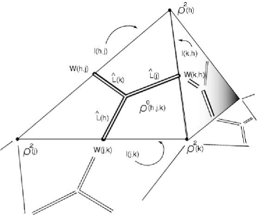
Figure 2.8: The relation between the edge-lengths of the conical polytope and the edge-lenghts of the triangulation.

which allows to recover, as the indices $(h,j,k)$ vary, the metric geometry of $|P_{T_{l}}|\rightarrow{M}$ and of its dual triangulation $|T_{l}|\rightarrow M$, from $((M;N_{0}),\mathcal{C});\{ds_{(k)}^{2}\})$ (see figure 2.8). In this sense, the stiffening [43] of $((M;N_{0}),\mathcal{C})$ defined by the punctured Riemann surface

$$((M;N_{0}),\mathcal{C});\{ds_{(k)}^{2}\})=$$ (2.46)

$$=\bigcup_{\{\rho^{0}(h,j,k)\}}^{N_{2}(T)}U_{\rho^{0}(h,j,k)}\bigcup_{\{\rho^{1}(h,j)\}}^{N_{1}(T)}U_{\rho^{1}(h,j)}\bigcup_{\{\rho^{2}(k)\}}^{N_{0}(T)}(\Delta_{k}^{\ast},ds_{(k)}^{2}),$$

is the uniformization of $((M;N_{0}),\mathcal{C})$ associated with the conical Regge polytope $|P_{l}|\rightarrow M$.

Although the correspondence between conical Regge polytopes and the above punctured Riemann surface is rather natural there is yet another uniformization representation of $|P_{l}|\rightarrow M$ which is of relevance in discussing conformal field theory on a given $|P_{l}|\rightarrow M$. The point is that the analysis of a CFT on a singular surface such as $|P_{l}|\rightarrow M$ calls for the imposition of suitable boundary conditions in order to take into account the conical singularities of the underlying Riemann surface $((M;N_{0}),\mathcal{C},ds^{2}_{(k)})$. This is a rather delicate issue since conical metrics give rise to difficult technical problems in discussing the glueing properties of the resulting conformal fields. In boundary conformal field theory, problems of this sort are taken care of (see e.g.[[44]]) by (tacitly) assuming that a neighborhood of the possible boundaries is endowed with a cylindrical metric. In our setting such a prescription naturally calls into play the metric associated with the quadratic differential $\phi$, and requires that we regularize into finite cylindrical ends the cones $(\Delta_{k}^{\ast},ds_{(k)}^{2})$.   Such a regularization is realized by noticing that if we introduce the annulus

$$\Delta_{\theta(k)}^{\ast}\doteq\left\{\zeta(k)\in\mathbb{C}|e^{-\frac{2\pi}{\theta(k)}}\leq|\zeta(k)|\leq 1\right\}\subset\overline{U_{\rho^{2}(k)}},$$ (2.47)

then the surface with boundary

$$M_{\partial}\doteq((M_{\partial};N_{0}),\mathcal{C})=\bigcup U_{\rho^{0}(j)}\bigcup U_{\rho^{1}(h)}\bigcup(\Delta_{\theta(k)}^{\ast},\phi(k))$$ (2.48)

defines the blowing up of the conical geometry of  $((M;N_{0}),\mathcal{C},ds_{(k)}^{2})$ along the ribbon graph $\Gamma$ (see figure 2.9).

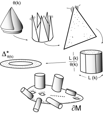
Figure 2.9: Blowing up the conical geometry of the polytope into finite cylindrical ends generates a uniformized Riemann surface with cylindrical boundaries.

The metrical geometry of  $(\Delta_{\theta(k)}^{\ast},\phi(k))$ is that of a flat cylinder with a circumference of length given by $L(k)$ and heigth given by $L(k)/\theta(k)$, (this latter being the slant radius of the generalized Euclidean cone $(\Delta_{k}^{\ast},ds_{(k)}^{2})$ of base circumference $L(k)$ and vertex conical angle $\theta(k)$).We also have

$$\partial M_{\partial} = \bigsqcup_{k=1}^{N_{0}}S_{\theta(k)}^{(+)},$$ (2.49)

$$\partial\Gamma = \bigsqcup_{k=1}^{N_{0}}S_{\theta(k)}^{(-)}$$

where the circles

$$S_{\theta(k)}^{(+)} \doteq \left\{\zeta(k)\in\mathbb{C}||\zeta(k)|=e^{-\frac{2\pi}{\theta(k)}}\right\},$$ (2.50)

$$S_{\theta(k)}^{(-)} \doteq \left\{\zeta(k)\in\mathbb{C}||\zeta(k)|=1\right\}$$

respectively denote the inner and the outer boundary of the annulus $\Delta_{\theta(k)}^{\ast}$. Note that by collapsing $S_{\theta(k)}^{(+)}$ to a point we get back the original cones $(\Delta_{k}^{\ast},ds_{(k)}^{2})$. Thus, the surface with boundary $M_{\partial}$ naturally corresponds to the ribbon graph $\Gamma$ associated with the 1-skeleton $K_{1}(|P_{T_{l}}|\rightarrow{M})$ of the polytope $|P_{T_{l}}|\rightarrow{M}$, decorated with the finite cylinders $\{\Delta_{\theta(k)}^{\ast},|\phi(k)|\}$. In such a framework the conical angles $\{\theta(k)=2\pi-\varepsilon(k)\}$ appears as (reciprocal of the) moduli $m_{k}$ of the annuli $\{\Delta_{\theta(k)}^{\ast}\}$,

$$m(k)=\frac{1}{2\pi}\ln\frac{1}{e^{-\frac{2\pi}{\theta(k)}}}=\frac{1}{\theta(k)}$$ (2.51)

(recall that the modulus of an annulus $r_{0}<|\zeta|<r_{1}$ is defined by $\frac{1}{2\pi}\ln\frac{r_{1}}{r_{0}}$). According to these remarks we can equivalently represent the conical Regge polytope $|P_{T_{l}}|\rightarrow{M}$ with the uniformization $((M;N_{0}),\mathcal{C});\{ds_{(k)}^{2}\})$ or with its blowed up version $M_{\partial}$.

Chapter 3 The WZW model on Random Regge Triangulations

The formulation of a conformal field theory and in particular of a WZW model over a triangulated Riemann surface has been a subject of great interests in the past years. As we have outilined in the introduction, despite several attempts starting directly from a Chern-Simons theory (see as an example [33]), many difficulties have arosen ranging from the dynamics of G-valued field to the non trivial dependance of the model from the underlying topology. In this chapter we will follow a complete different approach [31] defining the WZW model directly from the triangulated Riemann surface; in order to accomplish this task we will use the techniques introduced in the previous chapter which are more analytic in spirit and for this reason they allow us to avoid the natural difficulties raising from combinatorial calculus. Bearing in mind that our ultimate goal is to give an holographic description of the CS/WZW relation and to intepret the functional (1.32), we will specialize our analysis to the SU(2) model; we will also explicitly write the partition function for the theory at level $k=1$ which directly involves the $6j$ symbols of the quantum group at $q=\exp(i\frac{\pi}{3})$.

3.1 The WZW model on a Regge polytope

Let $G$ be a connected and simply connected Lie group. In order to make things simpler we shall limit our discussion to the case $G=SU(2)$, this being the case of more direct interest to us. Recall [44] that the complete action of the Wess-Zumino-Witten model on a closed Riemann surface $M$ of genus $g$ is provided by

$$S^{WZW}(h)=\frac{\kappa}{4\pi\sqrt{-1}}\int_{M}tr\left(h^{-1}\partial h\right)\left(h^{-1}\overline{\partial}h\right)+S^{WZ}(h),$$ (3.1)

where $h:M\rightarrow SU(2)$ denotes a $SU(2)$-valued field on $M$, $\kappa$ is a positive constant (the level of the model), $tr(\cdot)$ is the Killing form on the Lie algebra (normalized so that the root has length $\sqrt{2}$) and $S^{WZ}(h)$ is the topological Wess-Zumino term needed [54] in order to restore conformal invariance of the theory at the quantum level. Explicitly, $S^{WZ}(h)$ can be characterized by extending the field $h:M\rightarrow SU(2)$ to maps $\widetilde{h}:V_{M}\rightarrow SU(2)$ where $V_{M}$ is a three-manifold with boundary such that $\partial V_{M}=M$, and set

$$S^{WZ}(h)=\frac{\kappa}{4\pi\sqrt{-1}}\int_{V_{M}}\widetilde{h}^{\ast}\chi_{SU(2)},$$ (3.2)

where $\widetilde{h}^{\ast}\chi_{SU(2)}$ denotes the pull-back to $V_{M}$ of the canonical 3-form on $SU(2)$

$$\chi_{SU(2)}\doteq\frac{1}{3}tr\left(h^{-1}dh\right)\wedge\left(h^{-1}dh\right)\wedge\left(h^{-1}dh\right),$$ (3.3)

(recall that for $SU(2)$, $\chi_{SU(2)}$ reduces to $4\mu_{S^{3}}$, where $\mu_{S^{3}}$ is the volume form on the unit 3-sphere $S^{3}$). As is well known, $S^{WZ}(h)$ so defined depends on the extension $\widetilde{h}$ , the ambiguity being parametrized by the period of the form $\chi_{SU(2)}$ over the integer homology $H_{3}(SU(2))$. Demanding that the Feynman amplitude $e^{-S^{WZW}(h)}$ is well defined requires that the level $\kappa$ is an integer.

Figure 3.1: The geometrical set up for the WZW model. The surface M opens up to show the associated handlebody. The group SU(2) is here shown as the 3-sphere foliated into (squashed) 2-spheres.

3.1.1 Polytopes and the WZW model with boundaries

From the results discussed in the previous chapter, it follows that a natural strategy for introducing the WZW model on the Regge polytope $|P_{T_{l}}|\rightarrow{\ M}$ is to consider maps $h:M_{\partial}\rightarrow SU(2)$ on the associated surface with cylindrical boundaries $M_{\partial}\doteq((M_{\partial};N_{0}),\mathcal{C})$. Such maps $h$ should satisfy suitable boundary conditions on the (inner and outer) boundaries $\{S_{\theta(k)}^{(\pm)}\}$ of the annuli $\{\Delta_{\theta(k)}^{\ast}\}$, corresponding to the (given) values of the $SU(2)$ field on the boundaries of the cells of $|P_{T_{l}}|\rightarrow{\ M}$ and on their barycenters, (the field being free to fluctuate in the cells). Among all possible boundary conditions, there is a choice which is particularly simple and which allows us to reduce the study of WZW model on each given Regge polytopes to the (quantum) dynamics of WZW fields on the finite cylinders (annuli) $\{\Delta_{\theta(k)}^{\ast}\}$ decorating the ribbon graph $\Gamma$ and representing the conical cells of $|P_{T_{l}}|\rightarrow{\ M}$. Such an approach corresponds to first study the WZW model on $|P_{T_{l}}|\rightarrow{\ M}$ as a CFT. Its (quantum) states will then depend on the boundary conditions on the $SU(2)$ field $h$ on $\{S_{\theta(k)}^{(\pm)}\}$; roughly speaking such a procedure turns out to be equivalent to a prescription assigning an irreducible representation of $SU(2)$ to each barycenter of the given polytope $|P_{T_{l}}|\rightarrow{\ M}$. Such representations are parametrized by the boundary conditions which, by consistency, turn out to be necessarily quantized. They are also parametrized by elements of the geometry of $|P_{T_{l}}|\rightarrow{\ M}$, in particular by the deficit angles.

In order to carry over such a program, let us associate with each inner boundary $S_{\theta(i)}^{(+)}$ the $SU(2)$ Cartan generator

$$\Lambda_{i}\doteq\frac{\lambda(i)}{\kappa}\mathbf{\sigma}_{3}\text{, with\ }\mathbf{\sigma}_{3}=\left(\begin{array}[]{cc}1&0\\ 0&-1\end{array}\right)$$ (3.4)

where, for later convenience, $\lambda(i)\in\mathbb{R}$ has been normalized to the level $\kappa$,  and let

$$C_{i}^{(+)}\doteq\left\{\gamma e^{2\pi\sqrt{-1}\Lambda_{i}}\gamma^{-1}\;|\;\gamma\in SU(2)\right\}.$$ (3.5)

denote the (positively oriented) two-sphere $S^{2}_{\theta(i)}$ in $SU(2)$ representing the associated conjugacy class, (note that $C_{i}^{(+)}$ degenerates to a single point for the center of $SU(2)$). Such a prescription basically prevent out-flow of momentum across the boundary and has been suggested, in the framework of D-branes theory in [55], (see also [44]). Similarly, to the outer boundary $S_{\theta(i)}^{(-)}$ we associate the conjugacy class $C_{i}^{(-)}=\overline{C_{i}^{(+)}}$ describing the conjugate two-sphere $\overline{S^{2}_{\theta(i)}}$ (with opposite orientation) in $SU(2)$ associated with $S^{2}_{\theta(i)}$.  Given such data, we consider maps $h:M_{\partial}\rightarrow SU(2)$ that satisfy the fully symmetric boundary conditions (see figure 3.2) [56],

$$h(S_{\theta(i)}^{(\pm)})\subset C_{i}^{(\pm)}.$$ (3.6)

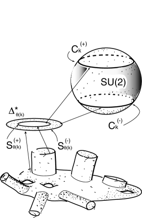
Figure 3.2: The geometrical setup for SU(2) boundary conditions on each $(\Delta_{\theta(k)}^{\ast},\phi(k))$ decorating the 1-skeleton of $|P_{T_{l}}|\rightarrow{M}$. For simplicity, the group SU(2) is incorrectly rendered; note that each circumference $C_{k}^{\pm}$ is actually a two-sphere, (or degenerates to a point).

Note that since $C_{i}^{(+)}$ and $C_{i}^{(-)}$ carry opposite orientations, the functions $h(S_{\theta(i)}^{(\pm)})$ are normalized to $h(S_{\theta(i)}^{(-)})h(S_{\theta(i)}^{(+)})={\mathbf{e}}$, (the identity $\in{SU(2)}$). The advantage of considering this subset of maps $h:M_{\partial}\rightarrow SU(2)$ is that when restricted to the boundary $\partial M_{\partial}$, (i.e., to the inner conjugacy classes $C_{i}^{(+)}$), the 3-form $\chi_{SU(2)}$ (3.3) becomes exact, and one can write

$$\left.\chi_{SU(2)}\right|_{C_{i}}=d\omega_{i},$$ (3.7)

where the 2-form $\omega_{i}$ is provided by

$$\omega_{i}=tr(\gamma^{-1}d\gamma)e^{2\pi\sqrt{-1}\Lambda_{i}}(\gamma^{-1}d\gamma)e^{-2\pi\sqrt{-1}\Lambda_{i}}.$$ (3.8)

In such a case, we can extend [44] the map $h:M_{\partial}\rightarrow SU(2)$ to a map ${\widehat{h}}:((M;N_{0}),\mathcal{C})\rightarrow SU(2)$ from the closed surface $((M;N_{0}),\mathcal{C})$ to $SU(2)$ in such a way that $\widehat{h}(\delta_{\theta(i)})\subset C_{i}^{(+)}$, where

$$\delta_{\theta(i)}\doteq\left\{\zeta(i)\in\mathbb{C}|\;|\zeta(i)|\leq e^{-\frac{2\pi}{\theta(i)}}\right\}$$ (3.9)

is the disk capping the cylindrical end $\{\Delta_{\theta(i)}^{\ast},|\phi(i)|\}$, (thus $\partial\delta_{\theta(i)}=S_{\theta(k)}^{(+)}$ and $\Delta_{\theta(i)}^{\ast}\cup\delta_{\theta(i)}\ \ \simeq\overline{U}_{\rho^{2}(i)}$). In this connection note that the boundary conditions $h(S_{\theta(i)}^{(+)})\subset C_{i}^{(+)}$ define elements of the loop group

$$\mathcal{L}_{(i)}SU(2)\doteq Map(S_{\theta(i)}^{(+)},SU(2))\simeq Map(S^{1},SU(2)).$$ (3.10)

Similarly, any other extension  $h^{\prime}_{i}=\widehat{h}_{i}g$, ($g\in SU(2)$), of $h$ over the capping disks $\delta_{\theta(i)}$, can be considered as an element of the group $Map(\delta_{\theta(i)},SU(2))$. In the same vein, we can interpret $\widetilde{h}_{i}=(\widehat{h}_{i},h_{i}^{\prime})$ as a map from the spherical double (see below) $S_{i}^{2}$ of $\delta_{\theta(i)}$ into $SU(2)$, i.e., as an element of the group $Map(S_{i}^{2},SU(2))$. It follows that each possible extension of  the boundary condition $h(S_{\theta(i)}^{(+)})$ fits into the exact sequence of groups

$$1\rightarrow Map(S_{i}^{2},SU(2))\rightarrow Map(\delta_{\theta(i)},SU(2))\rightarrow Map(S_{\theta(i)}^{(+)},SU(2))\rightarrow 1.$$ (3.11)

In order to discuss the properties of such extensions we can proceed as follows, (see [44] for the analysis of these and related issues in the general setting of boundary CFT).

Let us denote by $V_{M}$,  with $\partial V_{M}=((M,N_{0});\mathcal{C})$, the 3-dimensional handlebody associated with the surface $((M,N_{0});\mathcal{C})$, and corresponding to the mapping $\widehat{h}:((M,N_{0});\mathcal{C})\rightarrow SU(2)\simeq S^{3}$ thought of as an immersion in the 3-sphere. Since the conjugacy classes $C_{i}^{(+)}$ are 2-spheres and the homotopy group $\pi_{2}(SU(2))$ is trivial, we can further extend the maps $\widehat{h}$ to a smooth function $\ \widehat{H}:V_{M}\rightarrow SU(2)$, (thus, by construction  $\widehat{H}(\delta_{\theta(i)})\subset$ $C_{i}^{(+)}$). Any such an extension can be used to pull-back to the handlebody $V_{M}$ the Maurer-Cartan 3-form $\chi_{SU(2)}$ and it is natural to define the Wess-Zumino term associated with $((M,N_{0});\mathcal{C})$ according to

$$S_{|P_{T_{l}}|}^{WZ}(\widehat{h},\widehat{H})\doteq\frac{\kappa}{4\pi\sqrt{-1}}\int_{V_{M}}\widehat{H}^{\ast}\chi_{SU(2)}-\frac{\kappa}{4\pi\sqrt{-1}}\sum_{j=1}^{N_{0}}\int_{\delta_{\theta(j)}}\left.\widehat{h}\right|_{\delta_{\theta(j)}}^{\ast}\omega_{j}.$$ (3.12)

In general,  such a definition of  $S_{|P_{T_{l}}|}^{WZ}(\widehat{h},\widehat{H})$ depends on the particular extensions $(\widehat{h},\widehat{H})$ we are considering, and if we denote by $(h^{\prime}=\widehat{h}g,H^{\prime})$, $g\in SU(2)$, a different extension, then, by reversing the orientation of the handlebody $V_{M}$ and of the capping disks $\delta_{\theta(j)}$ over which $S_{|P_{T_{l}}|}^{WZ}(h^{\prime},H^{\prime})$ is evaluated, the difference between the resulting WZ terms can be written as

$$S_{|P_{T_{l}}|}^{WZ}(\widehat{h},\widehat{H})-S_{|P_{T_{l}}|}^{WZ}(h^{\prime},H^{\prime})=$$ (3.13)

$$=\frac{\kappa}{4\pi\sqrt{-1}}\left(\int_{V_{M}}\widehat{H}^{\ast}\chi_{SU(2)}+\int_{V_{M}^{(-)}}H^{\prime\ast}\chi_{SU(2)}\right)-$$

$$-\frac{\kappa}{4\pi\sqrt{-1}}\sum_{j=1}^{N_{0}}\left(\int_{\delta_{\theta(j)}}\left.\widehat{h}\right|_{\delta_{\theta(j)}}^{\ast}\omega_{j}+\int_{\delta_{\theta(j)}^{(-)}}\left.h^{\prime}\right|_{\delta_{\theta(j)}}^{\ast}\omega_{j}\right).$$

Note that

$$(V_{M},\widehat{H})\cup(V_{M}^{(-)},H^{\prime})=(\widetilde{V}_{M},\widetilde{H})$$ (3.14)

is the 3-manifold (ribbon graph) double of $V_{M}$  endowed with the extension $\widetilde{H}\doteq(\widehat{H},H^{\prime})$   and

$$(\delta_{\theta(j)},\widehat{h_{j}})\cup(\delta_{\theta(j)}^{(-)},h_{j}^{\prime})=(S_{j}^{2},\widetilde{h_{j}}),$$ (3.15)

are the 2-spheres defined by doubling the capping disks $\delta_{\theta(j)}$, decorated with the extension $\widetilde{h}_{j}\doteq(\widehat{h}_{j},h_{j}^{\prime})\in C_{j}^{(+)}$. By construction $(\widetilde{V}_{M},\widetilde{H})$ is such that $\partial(\widetilde{V}_{M},\widetilde{H})=\cup_{j=1}^{N_{0}}(S_{j}^{2},\widetilde{h_{j}})$ so that we can equivalently write (3.13) as

$$S_{|P_{T_{l}}|}^{WZ}(\widehat{h},\widehat{H})-S_{|P_{T_{l}}|}^{WZ}(h^{\prime},H^{\prime})=\frac{\kappa}{4\pi\sqrt{-1}}\int_{\widetilde{V}_{M}}\widetilde{H}^{\ast}\chi_{SU(2)}-$$ (3.16)

$$-\frac{\kappa}{4\pi\sqrt{-1}}\sum_{j=1}^{N_{0}}\int_{S_{j}^{2}}\widetilde{h}^{\ast}\omega_{j}.$$

To such an expression we add and subtract

$$\frac{\kappa}{4\pi\sqrt{-1}}\sum_{j=1}^{N_{0}}\int_{B_{j}^{3}}\widetilde{H_{j}}^{\ast}\chi_{SU(2)}$$ (3.17)

where $B_{j}^{3}$ are 3-balls such that $\partial B_{j}^{3}=S_{j}^{2(-)}$, (the boundary orientation is inverted so that we can glue such $B_{j}^{3}$ to the corresponding boundary components of $\widetilde{V}_{M}$), and $\widetilde{H_{j}}$ are corresponding extensions of $\widetilde{H}$ with $\widetilde{H_{j}}|_{S_{j}^{2}}=\widetilde{h}_{j}$. Since $\widetilde{V}_{M}\cup$ $B_{j}^{3}$ results in a closed 3-manifold $W^{3}$, we eventually get

$$S_{|P_{T_{l}}|}^{WZ}(\widehat{h},\widehat{H})-S_{|P_{T_{l}}|}^{WZ}(\eta)(h^{\prime},H^{\prime})=\frac{\kappa}{4\pi\sqrt{-1}}\int_{W^{3}}\widetilde{H}^{\ast}\chi_{SU(2)}-$$ (3.18)

$$-\frac{\kappa}{4\pi\sqrt{-1}}\sum_{j=1}^{N_{0}}\left(\int_{B_{j}^{3}}\widetilde{H_{j}}^{\ast}\chi_{SU(2)}-\int_{\partial B_{j}^{3}}\widetilde{h}^{\ast}\omega_{j}\right),$$

where we have rewritten the integrals over $S_{j}^{2}$ appearing in (3.16) as integrals over $\partial B_{j}^{3}=S_{j}^{2(-)}$, (hence the sign-change).  This latter expression shows that inequivalent extensions are parametrized by the periods of $(\chi_{SU(2)},\omega_{j})$ over the relative integer homology groups $H_{3}(SU(2),\cup_{j=1}^{N_{0}}C_{j})$. Explicitly, the first term provides

$$\frac{\kappa}{4\pi\sqrt{-1}}\int_{W^{3}}\widetilde{H}^{\ast}\chi_{SU(2)}=\frac{\kappa}{4\pi\sqrt{-1}}\int_{\widetilde{H}(W^{3})}\chi_{SU(2)}=\frac{\kappa}{4\pi\sqrt{-1}}\int_{S^{3}}\chi_{SU(2)}.$$ (3.19)

Since $\int_{S^{3}}\chi_{SU(2)}=8\pi^{2}$, we get $\frac{\kappa}{4\pi\sqrt{-1}}\int_{W^{3}}\widetilde{H}^{\ast}\chi_{SU(2)}=-2\pi\kappa\sqrt{-1}$ . Each addend in the second group of terms yields

$$\frac{\kappa}{4\pi\sqrt{-1}}\left(\int_{B_{j}^{3}}\widetilde{H_{j}}^{\ast}\chi_{SU(2)}-\int_{\partial B_{j}^{3}}\widetilde{h}^{\ast}\omega_{j}\right)=$$ (3.20)

$$=\frac{\kappa}{4\pi\sqrt{-1}}\left(\int_{\widetilde{H}_{j}(B_{j}^{3})}\chi_{SU(2)}-\int_{\widetilde{h}(\partial B_{j}^{3})}\omega_{j}\right).$$

The domain of integration $\widetilde{h}(\partial B_{j}^{3})$ is the 2-sphere  $C_{j}\subset SU(2)$ associated with the given conjugacy class, whereas $\widetilde{H}_{j}(B_{j}^{3})$ is one of the two 3-dimensional balls in $SU(2)$ with boundary $C_{j}$. In the defining representation of $SU(2)\doteq\{x_{0}\mathbf{I}+\sqrt{-1}\sum x_{k}\mathbf{\sigma}_{k}|\;x_{0}^{2}+\sum x_{k}^{2}=1\}$, the conjugacy classes $C_{j}$ are defined by $x_{0}=\cos\frac{2\pi\lambda(j)}{\kappa}$ with $0\leq\frac{2\pi\lambda(j)}{\kappa}\leq\pi$, whereas the two 3-balls $\widetilde{H}_{j}(B_{j}^{3})$ bounded by $C_{j}$ are defined by $x_{0}\geq\cos\frac{2\pi\lambda(j)}{\kappa}$ and $x_{0}\leq\cos\frac{2\pi\lambda(j)}{\kappa}$. An explicit computation [44] over the ball $x_{0}\geq\cos\frac{2\pi\lambda(j)}{\kappa}$ shows that (3.20) is provided by $-4\pi\lambda(j)\sqrt{-1}$, and by $4\pi\sqrt{-1}(\frac{\kappa}{2}-\lambda(j))$ for $x_{0}\leq\cos\frac{2\pi\lambda(j)}{\kappa}$,  respectively. From these remarks it follows that

$$S_{|P_{T_{l}}|}^{WZ}(\widehat{h},\widehat{H})-S_{|P_{T_{l}}|}^{WZ}(h^{\prime},H^{\prime})\in 2\pi\sqrt{-1}\mathbb{Z}$$ (3.21)

as long as $\kappa$ is an integer, and $0\leq\lambda(j)\leq\frac{\kappa}{2}$ with $\lambda(j)$ integer or half-integer; in such a case the exponential of  the WZ term $S_{|P_{T_{l}}|}^{WZ}(\widehat{h},\widehat{H})$ is independent from the chosen extensions $(\widehat{h},\widehat{H})$, and we can unambiguosly write $S_{|P_{T_{l}}|}^{WZ}(\widehat{h})$.

It follows from such remarks that we can define the $SU(2)$ WZW action on $|P_{T_{l}}|\rightarrow{M}$ according to

$$S_{|P_{T_{l}}|}^{WZW}(\widehat{h})\doteq\frac{\kappa}{4\pi\sqrt{-1}}\int_{((M;N_{0}),\mathcal{C})}tr\left(\widehat{h}^{-1}\partial\widehat{h}\right)\left(\widehat{h}^{-1}\overline{\partial}\widehat{h}\right)+S_{|P_{T_{l}}|}^{WZ}(\widehat{h}).$$ (3.22)

where the WZ term $S_{|P_{T_{l}}|}^{WZ}(\eta)$ is provided by (3.12). It is worthwhile stressing that the condition $0\leq\lambda(j)\leq\frac{\kappa}{2}$ plays here the role of a quantization condition on the possible set of boundary conditions allowable for the WZW model on $|P_{T_{l}}|\rightarrow{M}$. Qualitatively, the situation is quite similar to the dynamics of branes on group manifolds, where in order to have stable, non point-like branes, we need a non vanishing $B$-field generating a NSNS 3-form $H$, (see e.g. [57]), here provided by $\omega_{j}$ and $\chi_{SU(2)}$, respectively. In such a setting, stable branes on $SU(2)$ are either point-like (corresponding to elements in the center $\pm e$ of $SU(2)$), or 2-spheres associated with a discrete set of radii. In our approach, such branes appear as the geometrical loci describing boundary conditions for WZW fields evolving on singular Euclidean surfaces. It is easy to understand the connection between the two formalism: in our description of the $\kappa$-level $SU(2)$ WZW model on $|P_{T_{l}}|\rightarrow{M}$ we can interpret the $SU(2)$ field as parametrizing an immersion of $|P_{T_{l}}|\rightarrow{M}$ in $S^{3}$ (of radius $\simeq\sqrt{\kappa}$). In particular, the annuli $\Delta^{*}_{\theta(i)}$ associated with the ribbon graph boundaries $\{\partial\Gamma_{i}\}$ can be thought of as sweeping out in $S^{3}$ closed strings which couples with the branes defined by $SU(2)$ conjugacy classes.

3.2 The Quantum Amplitudes at k=1

We are now ready to discuss the quantum properties of the fields $\widehat{h}$ involved in the above characterization of the $SU(2)$ WZW action on $|P_{T_{l}}|\rightarrow{M}$. Such properties follow by exploiting the action of the (central extension of the) loop group $Map(S_{\theta(i)}^{(+)},SU(2))$ generated, on the infinitesimal level, by the conserved currents

$$J(\zeta(i))\doteq-\kappa\partial_{(i)}\widehat{h}_{i}\widehat{h}_{i}^{-1}$$ (3.23)

$$\overline{J}(\overline{\zeta}(i))\doteq\kappa\widehat{h}_{i}^{-1}\overline{\partial}_{(i)}\widehat{h}_{i},$$

where $\partial_{(i)}\doteq\partial_{\zeta(i)}$. By writing $J(\zeta(i))=J^{a}(\zeta(i))\mathbf{\sigma}_{a}$, we can introduce the corresponding modes $J_{n}^{a}(i)$, from the Laurent expansion in each disk $\delta_{\theta(i)}$,

$$J^{a}(\zeta(i))=\sum_{n\in\mathbb{Z}}\zeta(i)^{-n-1}J_{n}^{a}(i),$$ (3.24)

(and similarly for the modes $\overline{J}_{n}^{a}(i)$). The operator product expansion of the currents $J^{a}(\zeta(i))J^{a}(\zeta^{\prime}(i))$, (with $\zeta(i)$ and $\zeta^{\prime}(i)$ both in $\delta_{\theta(i)}$ ) yields [44] the commutation relations of an affine $\widehat{\mathfrak{su}}(2)$ algebra at the level $\kappa$, i.e.

$$\left[J_{n}^{a}(i),J_{m}^{b}(i)\right]=\sqrt{-1}\varepsilon_{abc}J_{n+m}^{c}(i)+\kappa n\delta_{ab}\delta_{n+m,0}.$$ (3.25)

According to a standard procedure, we can then construct the Hilbert space $\mathcal{H}_{(i)}$ associated with the WZW fields $\widehat{h}_{i}$ by considering unitary irreducible highest weight representations of the two commuting copies of the current algebra $\widehat{\mathfrak{su}}(2)$ generated by $J^{a}(\zeta(i))|_{S_{\theta(i)}^{(+)}}$ and $\overline{J^{a}}(\overline{\zeta}(i))|_{S_{\theta(i)}^{(+)}}$. Such representations are labelled by the level $\kappa$ and by the irreducible representations of $SU(2)$ with spin $0\leq\lambda(i)\leq\frac{\kappa}{2}$. Note in particular that for $\kappa=1$ every highest weight representation of  $\widehat{\mathfrak{su}}(2)_{\kappa=1}$ also provides a representation of Virasoro algebra $Vir$ with central charge $c=1$. In such a case the representations of $\widehat{\mathfrak{su}}(2)_{\kappa=1}$ can be decomposed into $\mathfrak{su}(2)\oplus Vir$, and, up to Hilbert space completion, we can write

$$\mathcal{H}_{(i)}=\bigoplus_{0\leq\lambda(i)\leq\frac{1}{2},0\leq n\leq\infty}\left(V_{\mathfrak{su}(2)}^{(n+\lambda(i))}\otimes\overline{V}_{\mathfrak{su}(2)}^{(n+\lambda(i))}\right)\otimes\left(\mathcal{H}_{(n+\lambda(i))^{2}}^{Vir}\otimes\overline{\mathcal{H}}_{(n+\lambda(i))^{2}}^{Vir}\right)$$ (3.26)

where $V_{\mathfrak{su}(2)}^{(n+\lambda(i))}$ denotes the $(2\lambda(i)+1)$ -dimensional spin $\lambda(i)$ representation of $\mathfrak{su}(2)$, and $\mathcal{H}_{(n+\lambda(i))^{2}}^{Vir}$ is the (irreducible highest weight) representation of the Virasoro algebra of weight $(n+\lambda(i))^{2}$. Since $0\leq\lambda(i)\leq\frac{1}{2}$, it is convenient to set

$$j_{i}\doteq n+\lambda(i)\in\frac{1}{2}\mathbb{Z}^{+}$$ (3.27)

(with $0\in\mathbb{Z}^{+}$), and rewrite (3.26) as

$$\mathcal{H}_{(i)}=\bigoplus_{j_{i},\widehat{j}_{i}\in\frac{1}{2}\mathbb{Z}^{+}}\left(V_{\mathfrak{su}(2)}^{j_{i}}\otimes\overline{V}_{\mathfrak{su}(2)}^{\widehat{j}_{i}}\right)\otimes\left(\mathcal{H}_{j_{i}^{2}}^{Vir}\otimes\overline{\mathcal{H}}_{\widehat{j}_{i}^{2}}^{Vir}\right),$$ (3.28)

with $j_{i}+\widehat{j}_{i}$ $\in\mathbb{Z}^{+}$, [58].  Owing to this particularly simple structure of the representation spaces $\mathcal{H}_{(i)}$, we shall limit our analysis to the case $\kappa=1$.

Since the boundary of $\partial M$ of the surface $M$ is defined by the disjoint union $\bigsqcup S_{\theta(i)}^{(+)}$ and the boundary $\partial\Gamma$  of the ribbon graph $\Gamma$  is provided by $\bigsqcup S_{\theta(i)}^{(-)}$, it follows that we can associate to both $\partial M$ and $\partial\Gamma$ the Hilbert space

$$\mathcal{H}(\partial M)\simeq\mathcal{H}(\partial\Gamma)=\bigotimes_{i=1}^{N_{0}}\mathcal{H}_{(i)}.$$ (3.29)

Let us denote by $\left|\widehat{h}(S_{\theta(i)}^{(+)})\right\rangle\in\mathcal{H}_{(i)}$ the Hilbert space state vector associated with the boundary condition $\widehat{h}(S_{\theta(i)}^{(+)})$ on the $i$-th boundary component $S_{\theta(i)}^{(+)}$ of $M_{\partial}$. According to the analysis of the previous section, the ribbon graph double $\widetilde{V}_{M}$ generates a Schottky  $M^{D}$ double of the surface with cylindrical boundaries $M_{\partial}$, ($M^{D}$ is the closed surface obtained by identifying $M_{\partial}$ with another copy $M_{\partial}^{\prime}$ of $M_{\partial}$ with opposite orientation along their common boundary $\bigsqcup S_{\theta(i)}^{(+)}$). Such $M^{D}$ carries an orientation reversing involution

$$\Upsilon:M^{D}\rightarrow M^{D},\;\Upsilon^{2}=id$$ (3.30)

that interchanges $M_{\partial}$ and $M_{\partial}^{\prime}$ and which has the boundary $\bigsqcup S_{\theta(i)}^{(+)}$ as its fixed point set. The request of preservation of conformal symmetry along $\bigsqcup S_{\theta(i)}^{(+)}$ under the anticonformal involution $\Upsilon$ requires that the state $\left|\widehat{h}(S_{\theta(i)}^{(+)})\right\rangle$ must satisfy the glueing condition $(\mathbb{L}_{n}-\overline{\mathbb{L}}_{-n})\left|\widehat{h}(S_{\theta(i)}^{(+)})\right\rangle=0$, where, for $n\neq 0$,

$$\mathbb{L}_{n}=\frac{1}{2+\kappa}\sum_{m=-\infty}^{\infty}J_{n-m}^{a}J_{m}^{a},$$ (3.31)

and similarly for $\overline{\mathbb{L}}_{-n}$.  The glueing conditions above can be solved mode by mode, and to each irreducible representation of the Virasoro algebra $\mathcal{H}_{j_{i}^{2}}^{Vir}$ and its conjugate $\overline{\mathcal{H}}_{\widehat{j}_{i}^{2}=j_{i}^{2}}^{Vir}$, labelled by the given $j_{i}\doteq n+\lambda(i)\in\frac{1}{2}\mathbb{Z}^{+}$, we can associate a set of conformal Ishibashi states parametrized by the $\mathfrak{su}(2)$ representations $V_{\mathfrak{su}(2)}^{j_{i}}\otimes V_{\mathfrak{su}(2)}^{j_{i}}$. Such states are usually denoted by

$$\left.\left|j_{i};m,n\right\rangle\right\rangle,\;\;m,n\in(-j_{i},-j_{i}+1,...,j_{i}-1,j_{i}),$$ (3.32)

and one can write [49]

$$\left|\widehat{h}(S_{\theta(i)}^{(+)})\right\rangle=\frac{1}{2^{\frac{1}{4}}}\sum_{j_{i};m,n}D_{m,n}^{j_{i}}(\widehat{h}(S_{\theta(i)}^{(+)}))\left.\left|j_{i};m,n\right\rangle\right\rangle,$$ (3.33)

where

$$D_{m,n}^{j_{i}}(\widehat{h}(S_{\theta(i)}^{(+)})) =\sum_{l=\max(0,n-m)}^{\min(j_{i}-m,j_{i}+n)}\frac{\left[(j_{i}+m)!(j_{i}-m)!(j_{i}+n)!(j_{i}-n)!\right]^{\frac{1}{2}}}{(j_{i}-m-l)!(j_{i}+n-l)!l!(m-n+l)!}\times$$ (3.34)

$$\times a^{j_{i}+n-l}\;d^{j_{i}-m-l}\;b^{l}\;c^{m-n+l},$$

is the $V_{\mathfrak{su}(2)}^{j_{i}}$-representation matrix associated with the $SU(2)$ element

$$\widehat{h}(S_{\theta(i)}^{(+)})=\left(\begin{array}[]{cc}a&b\\ c&d\end{array}\right)\in C_{i}^{(+)},$$ (3.35)

in the $C_{i}^{(+)}$ conjugacy class.

3.2.1 The Quantum Amplitudes for the cylindrical ends

With the above preliminary remarks along the way, let us consider explicitly the structure of the quantum amplitude associated with the WZW model defined by the action $S_{|P_{T_{l}}|}^{WZW}(\widehat{h})$. Formally, such an amplitude is provided by the functional integral

$$\left|\partial{M},\otimes_{i}\widehat{h}(S_{\theta(i)}^{(+)})\right\rangle=\int_{\{\widehat{h}|_{S_{\theta(i)}^{(\pm)}}\in C_{i}^{(\pm)}\}}e^{-S_{|P_{T_{l}}|}^{WZW}(\widehat{h})}D\widehat{h},$$ (3.36)

where the integration is over all the maps $\widehat{h}$ satisfying the boundary conditions $\{\widehat{h}|_{S_{\theta(i)}^{(\pm)}}\in C_{i}^{(\pm)}\}$, and where $D\widehat{h}$ is the local product $\prod_{\zeta\in((M;N_{0}),\mathcal{C})}d\widehat{h}(\zeta)$ over $((M;N_{0}),\mathcal{C})$ of the $SU(2)$ Haar measure. As the notation suggests, the formal expression (3.36) takes value in the Hilbert space $\mathcal{\ H}$. Let us recall that the fields $\widehat{h}$ are constrained over the disjoint boundary components of $\partial\Gamma$  to belong to the conjugacy classes $\{\widehat{h}|_{S_{\theta(i)}^{(-)}}\in C_{i}^{(-)}\}$. This latter remark implies that the maps $\widehat{h}$   fluctuate on the $N_{0}$ finite cylinders $\{\Delta_{\theta(i)}^{\ast}\}$ wheras on the ribbon graph $\Gamma$ they are represented by boundary operators which mediate the changes in the boundary conditions on adjacent boundary components $\{\partial{\Gamma}_{i}\}$ of $\Gamma$. In order to exploit such a factorization property of (3.36) the first step is the computation of the amplitude, (for each given index $i$), for the cylinder $\Delta_{\theta(i)}^{\ast}$ with in and out boundary conditions $\widehat{h}|_{S_{\theta(i)}^{(\pm)}}\in C_{i}^{(\pm)}$,

$$Z_{\Delta_{\theta(i)}^{\ast}}\doteq\int_{\widehat{h}|_{S_{i}^{(\pm)}}\in C_{i}^{(\pm)}}e^{-S^{WZW}(\widehat{h};\Delta_{\theta(i)}^{\ast})}D\widehat{h}$$ (3.37)

where $S^{WZW}(\widehat{h};\Delta_{\theta(i)}^{\ast})$ is the restriction to $\Delta_{\theta(i)}^{\ast}$ of $S_{|P_{T_{l}}|}^{WZW}(\widehat{h})$. If we introduce the Virasoro operator $\mathbb{L}_{0}(i)$ defined by

$$\mathbb{L}_{0}(i)=\frac{2}{2+\kappa}\sum_{m=0}^{\infty}J_{-m}^{a}(i)J_{m}^{a}(i).$$ (3.38)

and notice that $\mathbb{L}_{0}(i)+\overline{\mathbb{L}}_{0}(i)-\frac{c}{12}$ , defines the Hamiltonian of the WZW theory on the cylinder $\Delta_{\theta(i)}^{\ast}$, ($c=\frac{3\kappa}{2+\kappa}$ being the central charge of the SU(2) WZW theory), then we can explicitly write

$$Z_{\Delta_{\theta(i)}^{\ast}}(\{C_{i}^{(\pm)}\})=\langle\widehat{h}(S_{\theta(i)}^{(-)})|e^{-\frac{2\pi}{\theta(i)}(\mathbb{L}_{0}(i)+\overline{\mathbb{L}}_{0}(i)-\frac{c}{12})}|\widehat{h}(S_{\theta(i)}^{(+)})\rangle,$$ (3.39)

where $\langle\widehat{h}(S_{\theta(i)}^{(-)})|$ and $|\widehat{h}(S_{\theta(i)}^{(+)})\rangle$ respectively denote the Hilbert space vectors associated with the boundary conditions $h(S_{\theta(i)}^{(-)})$ and $h(S_{\theta(i)}^{(+)})$ and normalized to $\langle\widehat{h}(S_{\theta(i)}^{(-)})||\widehat{h}(S_{\theta(i)}^{(+)})\rangle=1$ , (a normalization that follows from the fact that $\widehat{h}(S_{\theta(i)}^{(-)})$ and $\widehat{h}(S_{\theta(i)}^{(+)})$ belong, by hypotheses, to the conjugated 2-spheres $C_{i}^{(-)}$ and $C_{i}^{(+)}$ in $SU(2)$).

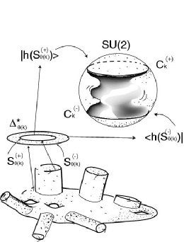
Figure 3.3: A pictorial rendering of the set up for computing the quantum amplitudes for the cylindrical ends associated with the surface $\partial M$.

The computation of the annulus partition function (3.39) has been explicitly carried out [49] for the boundary $SU(2)$ CFT at level $\kappa=1$. We restrict our analysis to this particular case and if we apply the results of [49], (see in particular eqn. (4.1) and the accompanying analysis) we get

$$Z_{\Delta_{\theta(i)}^{\ast}}(\{C_{i}^{\pm}\})=\\ =\frac{1}{\sqrt{2}}\sum_{j_{i}\in\frac{1}{2}\mathbb{Z}_{+}}\sum_{m,n}(-1)^{m-n}D_{-m,-n}^{j_{i}}(\widehat{h}^{-1}(S_{\theta(i)}^{(-)}))D_{m,n}^{j_{i}}(\widehat{h}(S_{\theta(i)}^{(+)}))\chi_{j_{i}^{2}}(e^{-\frac{4\pi}{\theta(i)}}),$$ (3.40)

where

$$\chi_{j_{i}^{2}}(e^{-\frac{4\pi}{\theta(i)}})=\frac{e^{-\frac{4\pi}{\theta(i)}j_{i}^{2}}-e^{-\frac{4\pi}{\theta(i)}(j_{i}+1)^{2}}}{\eta(e^{-\frac{4\pi}{\theta(i)}})}.$$ (3.41)

is the character of the Virasoro highest weight representation, and

$$\eta(q)\doteq q^{\frac{1}{24}}\prod_{n=1}^{\infty}(1-q^{n}),$$ (3.42)

is the Dedekind $\eta$-function.

By diagonalizing we can consider $h^{-1}(S_{\theta(i)}^{(-)})h(S_{\theta(i)}^{(+)})$ as an element of the maximal torus in $SU(2)$, i.e., we can write

$$h^{-1}(S_{\theta(i)}^{(-)})h(S_{\theta(i)}^{(+)})=\left(\begin{array}[]{cc}e^{4\pi\sqrt{-1}\lambda(i)}&0\\ 0&e^{-4\pi\sqrt{-1}\lambda(i)}\end{array}\right),$$ (3.43)

and a representation-theoretic computation [49] eventually provides

$$Z_{\Delta_{\theta(i)}^{\ast}}(\{C_{i}^{\pm}\})=\frac{1}{\sqrt{2}}\sum_{j\in\frac{1}{2}\mathbb{Z}_{+}}\cos(8\pi j_{i}\lambda(i))\frac{e^{-\frac{4\pi}{\theta(i)}j_{i}^{2}}}{\eta(e^{-\frac{4\pi}{\theta(i)}})}.$$ (3.44)

(Note that ${\alpha}$ in [49] corresponds to our $4\pi\sqrt{-1}\lambda(i)$, hence the presence of $\cos(8\pi j_{i}\lambda(i))$ in place of their $\cosh(2j_{i}\alpha(i))$).

An important point to stress is that, according to the above analysis, the partition function $Z_{\Delta_{\theta(i)}^{\ast}}(\{C_{i}^{\pm}\})$ can be interpreted as the superposition over all possible $j_{i}$ channel amplitudes

$$\partial\Gamma_{i}\longmapsto A(j_{i})\doteq\frac{1}{\sqrt{2}}\cos(8\pi j_{i}\lambda(i))\frac{e^{-\frac{4\pi}{\theta(i)}j_{i}^{2}}}{\eta(e^{-\frac{4\pi}{\theta(i)}})}$$ (3.45)

that can be associated to the boundary component $\partial\Gamma_{i}$ of the ribbon graph $\Gamma$. Such amplitudes can be interpreted as the various $j_{i}=(n+\lambda(i))$, ($0\leq\lambda(i)\leq\frac{1}{2}$), Virasoro (closed string) modes propagating along the cylinder $\Delta_{\theta(i)}^{\ast}$.

3.2.2 The Ribbon graph insertion operators

In order to complete the picture, we need to discuss how the $N_{0}$ amplitudes $\{A(j_{i})\}$ defined by (3.45) interact along $\Gamma$. Such an interaction is described by boundary operators which mediate the change in the boundary conditions $|\widehat{h}(S_{\theta(p)}^{(+)})\rangle_{\partial\Gamma_{p}}$ and $|\widehat{h}(S_{\theta(q)}^{(+)})\rangle_{\partial\Gamma_{q}}$ between any two adjacent boundary components $\partial\Gamma_{p}$ and $\partial\Gamma_{q}$, (note that the adjacent boundaries of the ribbon graph are associated with adjacent cells $\rho^{2}(p)$, $\rho^{2}(q)$ of  $|P_{T_{l}}|\rightarrow M$, and thus to the edges $\sigma^{1}(p,q)$ of the triangulation $|T_{l}|\rightarrow M$). In particular, the coefficients of the operator product expansion (OPE), describing the short-distance behavior of the boundary operators on adjacent $\partial\Gamma_{p}$ and $\partial\Gamma_{q}$, will keep tract of the combinatorics associated with $|P_{T_{l}}|\rightarrow{M}$.

To this end, let us consider generic pairwise adjacent 2-cells $\rho^{2}(p)$ , $\rho^{2}(q)$ and $\rho^{2}(r)$ in $|P_{T_{l}}|\rightarrow M$, and the associated cyclically ordered 3-valent vertex $\rho^{0}(p,q,r)\in|P_{T_{l}}|\rightarrow M$. Let $\{U_{\rho^{0}(p,q,r)},w\}$ the coordinate neighborhood of such a vertex, and $\{U_{\rho^{1}(p,q)},z\}$, $\{U_{\rho^{1}(q,r)},z\}$, and $\{U_{\rho^{1}(r,p)},z\}$ the neighborhoods of the corresponding oriented edges, (the $z$’s appearing in distinct $\{U_{\rho^{1}(\circ,\bullet)},z\}$ are distinct). Consider the edge $\rho^{1}(p,q)$ and two (infinitesimally neighboring) points $z_{1}=x_{1}+\sqrt{-1}y_{1}$ and $z_{2}=x_{2}+\sqrt{-1}y_{2}$, $\mathop{\mathrm{R}e}z_{1}=\mathop{\mathrm{R}e}z_{2}$, in the corresponding $U_{\rho^{1}(p,q)}$, with $x_{1}=x_{2}$. Thus, for $y_{1}\rightarrow 0^{+}$ we approach $\partial\Gamma_{p}\cap\rho^{1}(p,q)$ , whereas for $y_{2}\rightarrow 0^{-}$ we approach a point $\ \in\partial\Gamma_{q}\cap\rho^{1}(q,p)$.

Associated with the edge $\rho^{1}(p,q)\$ we have the two adjacent boundary conditions $|\widehat{h}(S_{\theta(p)}^{(+)})\rangle_{\partial\Gamma_{p}}$, and $|\widehat{h}(S_{\theta(q)}^{(+)})\rangle_{\partial\Gamma_{q}}$, respectively describing the given values of the field $\widehat{h}$ on the two boundary components $\partial\Gamma_{p}\cap\rho^{1}(p,q)$ and $\partial\Gamma_{q}\cap\rho^{1}(q,p)$ of $\rho^{1}(p,q)$. At the points $z_{1},z_{2}\in$ $U_{\rho^{1}(p,q)}$ we can consider the insertion of boundary operators $\psi_{j_{(p,q)}}^{j_{q}j_{p}}(z_{1})$ and $\psi_{j_{(q,p)}}^{j_{p}j_{q}}(z_{2})$ mediating between the corresponding boundary conditions, i.e.

$$\psi_{j_{(p,q)}}^{j_{q}j_{p}}(z_{1})|\widehat{h}(S_{\theta(p)}^{(+)})\rangle_{\partial\Gamma_{p}}\underset{y_{1}\rightarrow 0^{+}}{=}|\widehat{h}(S_{\theta(q)}^{(+)})\rangle_{\partial\Gamma_{q}},$$

(3.46)

$$\psi_{j_{(q,p)}}^{j_{p}j_{q}}(z_{2})|\widehat{h}(S_{\theta(q)}^{(+)})\rangle_{\partial\Gamma_{q}}\underset{y_{2}\rightarrow 0^{-}}{=}|\widehat{h}(S_{\theta(p)}^{(+)})\rangle_{\partial\Gamma_{p}}.$$

Note that $\psi_{j_{(p,q)}}^{j_{q}j_{p}}$ carries the single primary isospin label $j_{(p,q)}$ (also indicating the oriented edge $\rho^{1}(p,q)$ where we are inserting the operator), and the two additional isospin labels $j_{p}$ and $j_{q}$ indicating the two boundary conditions at the two portions of $\partial\Gamma_{p}$ and $\partial\Gamma_{q}$ adjacent to the insertion edge $\rho^{1}(p,q)$.  Likewise, by considering the oriented edges $\rho^{1}(q,r)$ and $\rho^{1}(r,p)$,  we can introduce the operators $\psi_{j_{(r,q)}}^{j_{q}j_{r}}$, $\psi_{j_{(q,r)}}^{j_{r}j_{q}}$, $\psi_{j_{(p,r)}}^{j_{r}j_{p}}$, and $\psi_{j_{(r,p)}}^{j_{p}j_{r}}$. In full generality, we can rewrite the above definition explicitly in terms of the adjacency matrix $B(\Gamma)$ of the ribbon graph $\Gamma$,

0otherwise,B_{st}(\Gamma)=\left\{\begin{tabular}[]{lll}$1$&if&$\rho^{1}(s,t)$ is an edge of $\Gamma$\\ &&\\ $0$&&otherwise\end{tabular}\right.,

1if ρ1(s,t) is an edge of Γ (3.47)

according to

$$\psi_{j_{(p,q)}}^{j_{q}j_{p}}(z_{1})|\widehat{h}(S_{\theta(p)}^{(+)})\rangle_{\partial\Gamma_{p}}\underset{y_{1}\rightarrow 0^{+}}{=}B_{pq}(\Gamma)|\widehat{h}(S_{\theta(q)}^{(+)})\rangle_{\partial\Gamma_{q}}.$$ (3.48)

Any such boundary operator, say $\psi_{j_{(p,q)}}^{j_{q}j_{p}}$, is a primary field (under the action of Virasoro algebra) of conformal dimension $H_{j_{(p,q)}}$, and they are all characterized [51], [50], [52] by the following properties dictated by conformal invariance (in the corresponding coordinate neighborhood $U_{\rho^{1}(p,q)}$, see figure 3.4)

$$\langle 0|\psi_{j_{(p,q)}}^{j_{q}j_{p}}(z_{1})|0\rangle=0,\;\;\langle\widehat{h}(S_{\theta(p)}^{(-)})|\mathbb{I}^{j_{p}j_{p}}|\widehat{h}(S_{\theta(p)}^{(+)})\rangle\;\!=a^{j_{p}j_{p}},$$

$$\langle 0|\psi_{j_{(p,q)}}^{j_{q}j_{p}}(z_{1})\psi_{j_{(q,p)}}^{j_{p}j_{q}}(z_{2})|0\rangle=b_{j_{(p,q)}}^{j_{q}j_{p}}|z_{1}-z_{2}|^{-2H_{j_{(p,q)}}}\delta_{j_{(p,q)}j_{(q,p)}},$$

where $\mathbb{I}^{j_{p}j_{p}}$ is the identity operator, and where $a^{j_{p}j_{p}}$ and $b_{j_{(p,q)}}^{j_{q}j_{p}}$ are normalization factors. In particular, the parameters $b_{j_{(p,q)}}^{j_{q}j_{p}}$ define the normalization of the two-points function. Note that [51] for $SU(2)$ the $b_{j_{(p,q)}}^{j_{q}j_{p}}$ are such that $b_{j_{(p,q)}}^{j_{q}j_{p}}=b_{j_{(q,p)}}^{j_{p}j_{q}}(-1)^{2j_{(p,q)}}$, and are (partially) constrained by the OPE of the $\psi_{j_{(p,q)}}^{j_{q}j_{p}}$. As customary in boundary CFT, we leave such a normalization factors dependence explicit in what follows.

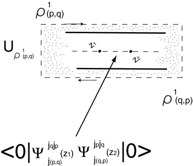
Figure 3.4: The insertion of boundary operators $\psi_{j_{(p,q)}}^{j_{q}j_{p}}$ in the complex coordinate neighborhood $U_{\rho^{1}(p,q)}$, giving rise to the two-point function in the corresponding oriented edge $\rho^{1}(p,q)$.

In order to discuss the properties of  the $\psi_{j_{(p,q)}}^{j_{q}j_{p}}$ , let us extend the (edges) coordinates $z$  to the unit disk  $U_{\rho^{0}(p,q,r)}$ associated to the generic vertex $\rho^{0}(p,q,r)$, and denote by

$$w_{p} = \frac{\varepsilon}{3}e^{\frac{1}{2}\pi\sqrt{-1}}\in U_{\rho^{0}(p,q,r)}\cap U_{\rho^{1}(p,q)}$$

$$w_{q} = \frac{\varepsilon}{2}e^{\frac{7}{6}\pi\sqrt{-1}}\in U_{\rho^{0}(p,q,r)}\cap U_{\rho^{1}(q,r)}$$ (3.50)

$$w_{r} = \varepsilon e^{\frac{11}{6}\pi\sqrt{-1}}\in U_{\rho^{0}(p,q,r)}\cap U_{\rho^{1}(r,p)}$$

the coordinates of three points in an $\varepsilon$- neighborhood ($0<\varepsilon<1$) of the vertex $w=0$, (fractions of $\varepsilon$ are introduced for defining a radial ordering; note also that by exploting the coordinate changes (2.38), one can easily map such points in the upper half planes associated with the edge complex variables $z$ corresponding to $U_{\rho^{1}(p,q)}$, $U_{\rho^{1}(q,r)}$, and $U_{\rho^{1}(r,p)}$, and formulate the theory in a more conventional fashion). To these points we associate the insertion of boundary operators $\psi_{j_{(r,p)}}^{j_{p}j_{r}}(w_{r})$, $\psi_{j_{(q,r)}}^{j_{r}j_{q}}(w_{q})$, $\psi_{j_{(p,q)}}^{j_{q}j_{p}}(w_{p})$ which pairwise mediate among the boundary conditions $|\widehat{h}(S_{\theta(p)}^{(+)})\rangle$, $|\widehat{h}(S_{\theta(q)}^{(+)})\rangle$, and $|\widehat{h}(S_{\theta(r)}^{(+)})\rangle$. The behavior of such insertions at the vertex $\rho^{0}(p,q,r)$, (i.e., as $\varepsilon\rightarrow 0$), is described by the following OPEs (see [50], [51])

$$\psi_{j_{(r,p)}}^{j_{p}j_{r}}(w_{r})\psi_{j_{(q,r)}}^{j_{r}j_{q}}(w_{q})=$$

$$=\sum_{j}C_{j_{(r,p)}j_{(q,r)}j}^{j_{p}j_{r}j_{q}}|w_{r}-w_{q}|^{H_{j}-H_{j_{(r,p)}}-H_{j_{(q,r)}}}(\psi_{j}^{j_{p}j_{q}}(w_{q})+...),$$

$$\psi_{j_{(q,r)}}^{j_{r}j_{q}}(w_{q})\psi_{j_{(p,q)}}^{j_{q}j_{p}}(w_{p})=$$

$$=\sum_{j}C_{j_{(q,r)}j_{(p,q)}j}^{j_{r}j_{q}j_{p}}|w_{q}-w_{p}|^{H_{j}-H_{j_{(q,r)}}-H_{j_{(p,q)}}}(\psi_{j}^{j_{r}j_{p}}(w_{p})+...),$$

$$\psi_{j_{(p,q)}}^{j_{q}j_{p}}(w_{p})\psi_{j_{(r,p)}}^{j_{p}j_{r}}(w_{r})=$$

$$=\sum_{j}C_{j_{(p,q)}j_{(r,p)}j}^{j_{q}j_{p}j_{r}}|w_{p}-w_{r}|^{H_{j}-H_{j_{(p,q)}}-H_{j_{(r,p)}}}(\psi_{j}^{j_{q}j_{p}}(w_{r})+...),$$

where the dots stand for higher order corrections in $|w_{\circ}-w_{\bullet}|$, the $H_{J_{...}}$ are the conformal weights of the corresponding boundary operators, and the $C_{j_{(r,p)}j_{(q,r)}j}^{j_{p}j_{r}j_{q}}$ are the OPE structure constants (see figure 3.5).

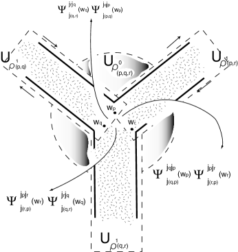
Figure 3.5: The OPEs between the boundary operators around a given vertex $\rho^{0}(p,q,r)$ in the corresponding complex coordinates neighborhoods $U_{\rho^{0}(p,q,r)}$, $U_{\rho^{1}(p,q)}$, etc..

As is well known [51], the parameters $b_{j_{(p,q)}}^{j_{q}j_{p}}$ and the constants $C_{j_{(r,p)}j_{(q,r)}j}^{j_{p}j_{r}j_{q}}$ are not independent. In our setting this is a consequence of the fact that to the oriented vertex $\rho^{0}(p,q,r)$ we can associate a three-point function which must be invariant under cyclic permutations, i.e.

$$\langle\psi_{j_{(r,p)}}^{j_{p}j_{r}}(w_{r})\psi_{j_{(q,r)}}^{j_{r}j_{q}}(w_{q})\psi_{j_{(p,q)}}^{j_{q}j_{p}}(w_{p})\rangle=\langle\psi_{j_{(p,q)}}^{j_{q}j_{p}}(w_{r})\psi_{j_{(r,p)}}^{j_{p}j_{r}}(w_{q})\psi_{j_{(q,r)}}^{j_{r}j_{q}}(w_{p})\rangle=$$

$$=\langle\psi_{j_{(q,r)}}^{j_{r}j_{q}}(w_{r})\psi_{j_{(p,q)}}^{j_{q}j_{p}}(w_{q})\psi_{j_{(r,p)}}^{j_{p}j_{r}}(w_{p})\rangle.$$

By using the boundary OPE (LABEL:OPE), each term can be computed in two distinct ways, e.g., by denoting with $\underbrace{}$ an OPE pairing, we must have

$$\langle\underbrace{\psi_{j_{(r,p)}}^{j_{p}j_{r}}(w_{r})\psi_{j_{(q,r)}}^{j_{r}j_{q}}(w_{q})}\psi_{j_{(p,q)}}^{j_{q}j_{p}}(w_{p})\rangle=\langle\psi_{j_{(r,p)}}^{j_{p}j_{r}}(w_{r})\underbrace{\psi_{j_{(q,r)}}^{j_{r}j_{q}}(w_{q})\psi_{j_{(p,q)}}^{j_{q}j_{p}}(w_{p})}\rangle$$ (3.55)

which (by exploiting (LABEL:twopoints)) in the limit $w\rightarrow 0$  provides

$$C_{j_{(r,p)}j_{(q,r)}j_{(p,q)}}^{j_{p}j_{r}j_{q}}b_{j_{(q,p)}}^{j_{p}j_{q}}=C_{j_{(q,r)}j_{(p,q)}j_{(r,p)}}^{j_{r}j_{q}j_{p}}b_{j_{(r,p)}}^{j_{p}j_{r}},$$ (3.56)

(note that the Kronecker $\delta$ in (LABEL:twopoints) implies that $j_{(q,p)}=j_{(p,q)}$, etc. ). From the OPE evaluation of the remaining two three-points function one similarly obtains

$$C_{j_{(p,q)}j_{(r,p)}j_{(q,r)}}^{j_{q}j_{p}j_{r}}b_{j_{(r,q)}}^{j_{q}j_{r}} = C_{j_{(r,p)}j_{(q,r)}j_{(p,q)}}^{j_{p}j_{r}j_{q}}b_{j_{(p,q)}}^{j_{q}j_{p}},$$

$$C_{j_{(q,r)}j_{(p,q)}j_{(r,p)}}^{j_{r}j_{q}j_{p}}b_{j_{(p,r)}}^{j_{r}j_{p}} = C_{j_{(p,q)}j_{(r,p)}j_{(q,r)}}^{j_{q}j_{p}j_{r}}b_{j_{(q,r)}}^{j_{r}j_{q}}.$$

Since

$$b_{j_{(q,p)}}^{j_{p}j_{q}} = b_{j_{(p,q)}}^{j_{q}j_{p}}(-1)^{2j_{(p,q)}},$$

$$b_{j_{(r,p)}}^{j_{p}j_{r}} = b_{j_{(p,r)}}^{j_{r}j_{p}}(-1)^{2j_{(p,r)}},$$ (3.58)

$$b_{j_{(q,r)}}^{j_{r}j_{q}} = b_{j_{(r,q)}}^{j_{q}j_{r}}(-1)^{2j_{(r,q)}},$$

one eventually gets

$$C_{j_{(r,p)}j_{(q,r)}j_{(p,q)}}^{j_{p}j_{r}j_{q}}b_{j_{(q,p)}}^{j_{p}j_{q}} = (-1)^{2j_{(q,p)}}C_{j_{(p,q)}j_{(r,p)}j_{(q,r)}}^{j_{q}j_{p}j_{r}}b_{j_{(q,r)}}^{j_{r}j_{q}},$$

$$C_{j_{(p,q)}j_{(r,p)}j_{(q,r)}}^{j_{q}j_{p}j_{r}}b_{j_{(r,q)}}^{j_{q}j_{r}} = (-1)^{2j_{(r,q)}}C_{j_{(q,r)}j_{(p,q)}j_{(r,p)}}^{j_{r}j_{q}j_{p}}b_{j_{(r,p)}}^{j_{p}j_{r}},$$ (3.59)

$$C_{j_{(q,r)}j_{(p,q)}j_{(r,p)}}^{j_{r}j_{q}j_{p}}b_{j_{(p,r)}}^{j_{r}j_{p}} = (-1)^{2j_{(p,r)}}C_{j_{(r,p)}j_{(q,r)}j_{(p,q)}}^{j_{p}j_{r}j_{q}}b_{j_{(p,q)}}^{j_{q}j_{p}},$$

which are the standard relation between the OPE parameters and the normalization of the 2-points function for boundary $SU(2)$ insertion operators, [51]. Such a lengthy (and slightly pedantic) analysis is necessary to show that our association of boundary insertion operators $\psi_{j_{(r,p)}}^{j_{p}j_{r}}$, to the edges of the ribbon graph $\Gamma$ is actually consistent with $SU(2)$ boundary CFT, in particular that geometrically the correlator $\langle\psi_{j_{(r,p)}}^{j_{p}j_{r}}(w_{r})\psi_{j_{(q,r)}}^{j_{r}j_{q}}(w_{q})\psi_{j_{(p,q)}}^{j_{q}j_{p}}(w_{p})\rangle$   is associated with the three mutually adjacent boundary components $\partial\Gamma_{p}$, $\partial\Gamma_{q}$, and $\partial\Gamma_{r}$ of the ribbon graph $\Gamma$. More generally, let us consider four mutually adjacent boundary components $\partial\Gamma_{p}$, $\partial\Gamma_{q}$, $\partial\Gamma_{r}$, and $\partial\Gamma_{s}$. Their adjacency relations can be organized in two distinct ways labelled by the distinct two vertices they generate: if $\partial\Gamma_{p}$ is adjacent to $\partial\Gamma_{r}$ then  we have the two vertices $\rho^{0}(p,q,r)$ and $\rho^{0}(p,r,s)$ connected by the edge $\rho^{1}(p,r)$; conversely, if $\partial\Gamma_{q}$ is adjacent to $\partial\Gamma_{s}$ then  we have the two vertices $\rho^{0}(p,q,s)$ and $\rho^{0}(q,r,s)$ connected by the edge $\rho^{1}(q,s)$.  It follows that the correlation function of the corresponding four boundary operators, $\langle\psi_{j_{(s,p)}}^{j_{p}j_{s}}\psi_{j_{(r,s)}}^{j_{s}j_{r}}\psi_{j_{(q,r)}}^{j_{r}j_{q}}\psi_{j_{(p,q)}}^{j_{q}j_{p}}\rangle$, can be evaluated by exploiting the ($(S)$-channel) factorization associated with the coordinate neighborhood $\{U_{\rho^{1}(r,p)},z^{(S)}\}$, or, alternatively, by exploiting the ($(T)$-channel) factorization associated with $\{U_{\rho^{1}(q,s)},z^{(T)}\}$ (see figure 3.6).

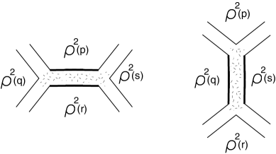
Figure 3.6: The dual channels in evaluating the correlation function of the four boundary operators corresponding to the four boundary components involved.

From the observation that both such expansions must yield the same result, it is possible [52] to directly relate the OPE coefficients $C_{j_{(r,p)}j_{(q,r)}j_{(p,q)}}^{j_{p}j_{r}j_{q}}$ with the fusion matrices $F_{j_{r}j_{(p,q)}}\left[\begin{array}[]{cc}j_{p}&j_{q}\\ j_{(r,p)}&j_{(q,r)}\end{array}\right]$ which express the crossing duality between four-points conformal blocks. Recall that for WZW models the fusion ring can be identified with the character ring of the quantum deformation $\mathcal{U}_{Q}(\mathbf{g})$ of  the enveloping algebra of $\mathbf{g}$ evaluated at the root of unity given by $Q=e^{\pi\sqrt{-1}/(\kappa+h^{\vee})}$ (where $h^{\vee}$ is the dual Coxeter number and $\kappa$ is the level of the theory). In other words, for WZW models, the fusion  matrices are the $6j$ -symbols of the corresponding (quantum) group. From such remarks, it follows that in our case (i.e., for $\kappa=1$, $h^{\vee}=2$) the structure constants $C_{j_{(r,p)}j_{(q,r)}j_{(p,q)}}^{j_{p}j_{r}j_{q}}$ are suitable entries [53] of the $6j$-symbols of the quantum group $SU(2)_{Q=e^{\frac{\pi}{3}\sqrt{-1}}}$, i.e.

$$C_{j_{(r,p)}j_{(q,r)}j_{(p,q)}}^{j_{p}j_{r}j_{q}}=\left\{\begin{array}[]{ccc}j_{(r,p)}&j_{p}&j_{r}\\ j_{q}&j_{(q,r)}&j_{(p,q)}\end{array}\right\}_{Q=e^{\frac{\pi}{3}\sqrt{-1}}}$$ (3.60)

3.2.3 The partition function.

The final step in our construction is to uniformize the local coordinate representation of the ribbon graph $\Gamma$ with the cylindrical metric $\{|\phi(i)|\}$, defined by the quadratic differential $\{\phi(i)\}$. In such a framework, there is a natural prescription for associating to the resulting metric ribbon graph $(\Gamma,\{|\phi(i)|\})$ a factorization of the correlation functions of   the $N_{1}$ insertion operators $\{\psi_{j_{(p,q)}}^{j_{q}j_{p}}\}$, (recall that $N_{1}$ is the number of edges of $\Gamma$). Explicitly, for the generic vertex  $\rho^{0}(p,q,r)$, let  $z_{p}^{(0)}\in U_{\rho^{1}(p,q)}\cap U_{\rho^{0}(p,q,r)}$,  $z_{q}^{(0)}\in U_{\rho^{1}(q,r)}\cap U_{\rho^{0}(p,q,r)}$, and  $z_{r}^{(0)}\in U_{\rho^{1}(r,p)}\cap U_{\rho^{0}(p,q,r)}$ respectively denote the coordinates of the points $w_{p}$, $w_{q}$, and $w_{r}$ (see (3.50)) in the respective edge uniformizations, and for notational purposes, let us set, (in an $\varepsilon$-neighborhood of $z_{\rho^{0}(p,q,r)}=0\in U_{\rho^{0}(p,q,r)}$),

$$\psi_{j_{(r,p)}}^{j_{p}j_{r}}(\rho^{0}(p,q,r)) \doteq \psi_{j_{(r,p)}}^{j_{p}j_{r}}(z_{r}^{(0)}),$$

$$\psi_{j_{(q,r)}}^{j_{r}j_{q}}(\rho^{0}(p,q,r)) \doteq \psi_{j_{(q,r)}}^{j_{r}j_{q}}(z_{q}^{(0)}),$$ (3.61)

$$\psi_{j_{(p,q)}}^{j_{q}j_{p}}(\rho^{0}(p,q,r)) \doteq \psi_{j_{(p,q)}}^{j_{q}j_{p}}(z_{p}^{(0)}).$$

Let us consider, (in the limit $\varepsilon\rightarrow 0$ ), the correlation function

$$\left\langle\bigotimes_{i=1}^{N_{0}(T)}\partial\Gamma_{i};\otimes j_{i}\right\rangle\doteq$$

$$\doteq\left\langle\prod_{\{\rho^{0}(p,q,r)\}}^{N_{2}(T)}\psi_{j_{(r,p)}}^{j_{p}j_{r}}(\rho^{0}(p,q,r))\psi_{j_{(q,r)}}^{j_{r}j_{q}}(\rho^{0}(p,q,r))\psi_{j_{(p,q)}}^{j_{q}j_{p}}(\rho^{0}(p,q,r))\right\rangle,$$

where  the product runs over the $N_{2}(T)$ vertices $\{\rho^{0}(p,q,r)\}$  of $\Gamma$. We can factorize it along the $N_{1}(T)$ channels generated by the edge cordinate neighborhoods $\{U_{\rho^{1}(p,q)}\}$ according to

$$\left\langle\bigotimes_{i=1}^{N_{0}(T)}\partial\Gamma_{i};\otimes j_{i}\right\rangle=$$

$$=\sum_{\{j_{(r,p)}\}}\prod_{\{\rho^{0}(p,q,r)\}}^{N_{2}(T)}\underset{\rho^{0}(p,q,r)}{\left\langle\psi_{j_{(r,p)}}^{j_{p}j_{r}}\psi_{j_{(q,r)}}^{j_{r}j_{q}}\psi_{j_{(p,q)}}^{j_{q}j_{p}}\right\rangle}\prod_{\{\rho^{1}(p,r)\}}^{N_{1}(T)}\underset{\rho^{1}(p,r)}{\left\langle\psi_{j_{(r,p)}}^{j_{p}j_{r}}\psi_{j_{(p,r)}}^{j_{r}j_{p}}\right\rangle}$$

where we have set

$$\underset{\rho^{0}(p,q,r)}{\left\langle\psi_{j_{(r,p)}}^{j_{p}j_{r}}\psi_{j_{(q,r)}}^{j_{r}j_{q}}\psi_{j_{(p,q)}}^{j_{q}j_{p}}\right\rangle}\doteq$$

$$\doteq\left\langle\psi_{j_{(r,p)}}^{j_{p}j_{r}}(\rho^{0}(p,q,r))\psi_{j_{(q,r)}}^{j_{r}j_{q}}(\rho^{0}(p,q,r))\psi_{j_{(p,q)}}^{j_{q}j_{p}}(\rho^{0}(p,q,r))\right\rangle,$$

$$\underset{\rho^{1}(p,r)}{\left\langle\psi_{j_{(r,p)}}^{j_{p}j_{r}}\psi_{j_{(p,r)}}^{j_{r}j_{p}}\right\rangle}\doteq\left\langle\psi_{j_{(r,p)}}^{j_{p}j_{r}}(\rho^{0}(p,q,r))\psi_{j_{(p,r)}}^{j_{r}j_{p}}(\rho^{0}(p,r,s))\right\rangle,$$ (3.65)

and where the summation runs over all $N_{1}(T)$ primary highest weight representation $\widehat{\mathfrak{su}}(2)_{\kappa=1}$, labelling the intermediate edge channels $\{j_{(r,p)}\}$. Note that according to (LABEL:twopoints) we can write

$$\underset{\rho^{1}(p,r)}{\left\langle\psi_{j_{(r,p)}}^{j_{p}j_{r}}\psi_{j_{(p,r)}}^{j_{r}j_{p}}\right\rangle}=b_{j_{(r,p)}}^{j_{p}j_{r}}L(p,r)^{-2H_{j_{(r,p)}}},$$ (3.66)

(recall that $j_{(r,p)}=j_{(p,r)}$), where $L(p,r)$ denotes the length of the edge $\rho^{1}(p,r)$ in the uniformization $(U_{\rho^{1}(p,r)},\{|\phi(i)|\})$. Moreover,  since (see (3.56))

$$\underset{\rho^{0}(p,q,r)}{\left\langle\psi_{j_{(r,p)}}^{j_{p}j_{r}}\psi_{j_{(q,r)}}^{j_{r}j_{q}}\psi_{j_{(p,q)}}^{j_{q}j_{p}}\right\rangle}=C_{j_{(r,p)}j_{(q,r)}j_{(p,q)}}^{j_{p}j_{r}j_{q}}b_{j_{(q,p)}}^{j_{p}j_{q}},$$ (3.67)

we get for the boundary operator correlator associated with the ribbon graph $\Gamma$ the expression

$$\left\langle\bigotimes_{i=1}^{N_{0}(T)}\partial\Gamma_{i};\otimes j_{i}\right\rangle=$$

$$=\sum_{\{j_{(r,p)}\}}\prod_{\{\rho^{0}(p,q,r)\}}^{N_{2}(T)}C_{j_{(r,p)}j_{(q,r)}j_{(p,q)}}^{j_{p}j_{r}j_{q}}b_{j_{(q,p)}}^{j_{p}j_{q}}\prod_{\{\rho^{1}(p,r)\}}^{N_{1}(T)}b_{j_{(r,p)}}^{j_{p}j_{r}}L(p,r)^{-2H_{j_{(r,p)}}}.$$

By identifying each $C_{j_{(r,p)}j_{(q,r)}j_{(p,q)}}^{j_{p}j_{r}j_{q}}$ with the corresponding $6j$-symbol, and observing that each normalization factor $b_{j_{(q,p)}}^{j_{p}j_{q}}$ occurs exactly twice, we eventually obtain

$$\left\langle\bigotimes_{i=1}^{N_{0}(T)}\partial\Gamma_{i};\otimes j_{i}\right\rangle=\sum_{\{j_{(r,p)}\}}\prod_{\{\rho^{0}(p,q,r)\}}^{N_{2}(T)}\left\{\begin{array}[]{ccc}j_{(r,p)}&j_{p}&j_{r}\\ j_{q}&j_{(q,r)}&j_{(p,q)}\end{array}\right\}_{Q=e^{\frac{\pi}{3}\sqrt{-1}}}\cdot$$ (3.71)

$$\cdot\prod_{\{\rho^{1}(p,r)\}}^{N_{1}(T)}\left(b_{j_{(r,p)}}^{j_{p}j_{r}}\right)^{2}L(p,r)^{-2H_{j_{(r,p)}}}.$$

As the notation suggests, such a correlator has a residual dependence on the representation labels $\{j_{i}\}$. In other words, it can be considered as an element of the tensor product $\mathcal{H}(\partial\Gamma)=$ $\otimes_{i=1}^{N_{0}(T)}\mathcal{H}_{(i)}$. It is then natural to interpret its evaluation over the amplitudes $\{A(j_{i})\}$ defined by ( 3.45) as the partition function $Z^{WZW}(|P_{T_{l}}|,\{\widehat{h}(S_{\theta(i)}^{(+)})\})$ associated with the quantum amplitude (3.36), and describing the $SU(2)$ WZW model (at level $\kappa=1$) on a random Regge polytope $|P_{T_{l}}|\rightarrow M$. By inserting the $N_{0}(T)$ amplitudes $\{A(j_{i})\}$ into (3.71), and summing over all possible representation indices $\{j_{p}\}$ we immediately get

$$Z^{WZW}(|P_{T_{l}}|,\{\widehat{h}(S_{\theta(i)}^{(+)})\})=$$

$$=\left(\frac{1}{\sqrt{2}}\right)^{N_{0}(T)}\sum_{\{j_{p}\in\frac{1}{2}\mathbb{Z}_{+}\}}\sum_{\{j_{(r,p)}\}}\prod_{\{\rho^{0}(p,q,r)\}}^{N_{2}(T)}\left\{\begin{array}[]{ccc}j_{(r,p)}&j_{p}&j_{r}\\ j_{q}&j_{(q,r)}&j_{(p,q)}\end{array}\right\}_{Q=e^{\frac{\pi}{3}\sqrt{-1}}}\cdot$$ (3.74)

$$\cdot\prod_{\{\rho^{1}(p,r)\}}^{N_{1}(T)}\left(b_{j_{(r,p)}}^{j_{p}j_{r}}\right)^{2}L(p,r)^{-2H_{j_{(r,p)}}}\cos(8\pi j_{p}\lambda(i))\frac{e^{-\frac{4\pi}{\theta(i)}j_{p}^{2}}}{\eta(e^{-\frac{4\pi}{\theta(i)}})},$$

where the summation $\sum_{\{j_{p}\in\frac{1}{2}\mathbb{Z}_{+}\}}$ is over all possible $N_{0}(T)$ channels $j_{p}$ describing the Virasoro (closed string) modes propagating along the cylinders $\{\Delta_{\theta(p)}^{\ast}\}_{p=1}^{N_{0}(T)}$. This is the partition function of our WZW model on a random Regge triangulation. The WZW fields are still present through their boundary labels $\lambda(i)$, (which can take the values $0,1/2$), wheras the metric geometry of the polytope enters explicitly both with the edge-length terms $L(p,r)^{-2H_{j_{(r,p)}}}$ and with the conical angle factors $\frac{e^{-\frac{4\pi}{\theta(i)}j_{p}^{2}}}{\eta(e^{-\frac{4\pi}{\theta(i)}})}$. The expression of $Z^{WZW}(|P_{T_{l}}|,\{\widehat{h}(S_{\theta(i)}^{(+)})\})$, also shows the mechanism through which the $SU(2)$ fields couple with simplicial curvature: the coupling amplitudes $\{A(j_{i})\}$ can be interpreted as describing a closed string emitted by $\partial\Gamma_{i}\simeq S_{\theta(i)}^{(-)}$, or rather by the $\overline{S_{\theta(i)}^{2}}$  brane image of this boundary component in $SU(2)$, and absorbed by the brane $S_{\theta(i)}^{2}$ image of the outer boundary $S_{\theta(i)}^{(+)}$, (the curvature carrying vertex). This exchange of closed strings between $2$-branes in  $SU(2)\simeq S^{3}$ describes the interaction of the quantum $SU(2)$ field with the classical gravitational background associated with the edge-length assignments $\{L(p,r)\}$, and with the deficit angles $\{\varepsilon(i)\doteq 2\pi-\theta(i)\}$.

Chapter 4 Holography and asymptotically flat space-times

One of the key success of the holographic principle is the chance to reconstruct spacetime starting from datas living on the boundary. The classical example is the AdS/CFT correspondence [10] where an equivalence between partition functions of a theory living in the bulk and in the boundary is imposed. More precisely the latter, in asymptotically AdS space-times, is strictly related to a gauge theory carrying indices of the asymptotic symmetry group (the conformal group).

This kind of relation has been mainly studied in the AdS case (and with less success also in dS spacetimes [16]) but no real attempt until now has been done in aymptotically flat space-times. Thus, the purpose of this chapter will be the study of the asymptotic symmetry group of asymptotically flat space-times (the Bondi-Metzner-Sachs group) as a candidate for the gauge group of the holographic boundary theory. Furthermore we will show the differences araising from the AdS case emphasizing in particular the failure of a unique geometric reconstruction of an asymptotically flat space-time.

4.1 Emergence of the BMS group in asymptotically flat spacetimes

In this section we briefly revisit the derivation of the BMS group and some of its properties. As said, the BMS group represents the ASG of asymptotically flat spacetimes. More properly it is a transformation pseudo-group of asymptotic isometries of the region close to infinity of the asymptotically flat (lorentzian) spacetimes . There is however a derivation proposed by Penrose as a group of transformations living intrinsically on $\Im$. In this case the BMS group is the transformation group on the boundary $\Im$.

From the point of view of the holographic principle we are interested in the theory living on the boundary and its symmetry group. We therefore prefer to consider this “boundary description” of the BMS group as more relevant and fundamental for our purposes. Moreover, it keeps into account the degenerate nature of $\Im$, which one has to face up when choosing a null screen. For completeness, however, we review various derivations.

4.1.1 BMS as asymptotic symmetry group

The BMS group was originally discovered [17], [59] by studying gravitational radiation emitted by bounded systems in asymptotically flat spacetimes; it is the group leaving invariant the asymptotic form of the metric describing these processes. Quite generally, one can choose $(u,r,\theta,\phi)$ coordinates close to null infinity and check that the components of the metric tensor behave like those of the Minkowski metric in null polar coordinates in the limit $r\rightarrow\infty$.

A BMS transformation $(\alpha,\Lambda)$ is then

$$\bar{u}=[K_{\Lambda}(x)]^{-1}(u+\alpha(x))+O(1/r)$$ (4.1)

$$\bar{r}=K_{\Lambda}(x)r+J(x,u)+O(1/r)$$ (4.2)

$$\bar{\theta}=(\Lambda x)_{\theta}+H_{\theta}(x,u)r^{-1}+O(1/r)$$ (4.3)

$$\bar{\phi}=(\Lambda x)_{\phi}+H_{\phi}(x,u)r^{-1}+O(1/r)$$ (4.4)

where $x$ is a point on the two sphere $S^{2}$ with coordinates $(\theta,\phi)$, $\Lambda$ represents a Lorentz transformation acting on $S^{2}$ as a conformal transformation and $K_{\Lambda}(x)$ is the corresponding conformal factor. Furthermore $\alpha$ is a scalar function on $S^{2}$ associated with the so called supertranslation subgroup. It represents the “size” of the group as we will see below.

The other functions are uniquely determined by $(\alpha,\Lambda)$ imposing

$$(\alpha_{1},\Lambda_{1})(\alpha_{2},\Lambda_{2})=(\alpha_{1}+\Lambda_{1}\alpha_{2},\Lambda_{1}\Lambda_{2})$$ (4.5)

$$(\Lambda_{1}\alpha_{2})(x)=[K_{\Lambda}(x)]^{-1}\alpha_{2}(\Lambda_{1}^{-1}x)$$ (4.6)

One immediately notices from (4.5) the structure of semidirect product. Therefore the BMS group $B=N\ltimes L$ is the semidirect product of the infinite dimensional supertranslation group $N$ with (the connected component of the homogeneous) Lorentz transformations group $L$.

An important point to keep in mind is that the ASG thus defined is universal since one gets the same group for all asymptotically flat spacetimes. This is quite surprising. In addition, the group is infinite dimensional due to the presence of extra symmetries which reflect the presence of gravity in the bulk.

It is also possible [60] to derive the BMS group B working in the unphysical spacetime and imposing differential and topological requirements on $\Im$, avoiding then asymptotic series expansions. In a sense, this is a finite version of the original BMS derivation, since one constructs a so called conformal Bondi frame in some finite neighborhood of $\Im$ and this finite region corresponds to an infinite region of the original physical spacetime.

Even if one is not working with an asymptotic expansion, we prefer to consider this derivation from a slightly different perspective with respect to the one of Penrose, who considers the emergence of the BMS working intrinsically on $\Im$. Actually, we are still working asymptotically, even if, in the unphysical space, the “infinite is brought to finite”. Recall, however, that had we chosen another conformal frame we would have obtained an isomorphic group. In other words, covariance is preserved by differentiable transformations acting on $\Im$. This indeed motivated Penrose to work directly on the geometrical properties of $\Im$ as we will see below and it seems more convenient to investigate the holographic principle in this context.

Choosing $x^{0}=u$, $x^{A}=(\theta,\phi)$ as coordinates on $\Im^{+}$ and $x^{1}=r$ defining the inverse luminosity distance, the (unphysical) metric $g^{\mu\nu}$ in the conformal Bondi frame is thus

$$g^{\mu\nu}=\left[\begin{array}[]{ccc}0&g^{01}&0\\ g^{01}&g^{11}&g^{1A}\\ 0&g^{1A}&g^{AB}\end{array}\right]$$

Using the freedom of gauge choice of the conformal factor and imposing global and asymptotic requirements on $\Im$ one can write the metric (in a neighbourhood of $\Im$) as

$$g^{\mu\nu}=\left[\begin{array}[]{ccc}0&1&0\\ 1&0&0\\ 0&0&q^{AB}\end{array}\right]$$

where $q^{AB}$ is the metric on the $S^{2}$ therefore time independent. One can eventually compute the generators $\xi^{\mu}$ of asymptotic infinitesimal transformations $x^{\mu}\rightarrow x^{\mu}+\xi^{\mu}$ by solving

$$\xi^{(\mu;\nu)}-(\Omega,_{\rho}\xi^{\rho}/\Omega)g^{\mu\nu}=0.$$ (4.7)

One finds

$$\xi^{A}=f^{A}(x^{B})$$ (4.8)

$$\xi^{0}=\frac{1}{2}uf_{;A}^{A}+\alpha(x^{B}),\;\xi^{1}=0.$$ (4.9)

Setting the supertranslations $\alpha(x^{A})$ to zero we get the (orthochronous) Lorentz group while setting the $f^{A}$ to zero we get the group of supetranslations as expected.

These are exactly the Killing vectors found by Sachs [59] in studying radiation at null infinity. However, one interprets the notion of asymptotic symmetry as follows: one declares an infinitesimal asymptotic symmetry to be described by a vector field $\xi^{a}$ (more precisely an equivalence of vector fields in the physical spacetime) such that the Killing equation $L_{\xi}g_{\mu\nu}=0$ is satisfied to as good an approximation as possible as one moves towards $\Im$.

One can also consider another derivation of the BMS group proposed by Geroch [61]. In a nutshell, this procedure considers the ASG as the group of consometries of $\Im$, i.e. conformally invariant structures associated with $\Im$. More properly, these structures live on the so called “asymptotic geometry”, a 3 dimensional manifold diffeomorphic to $\Im$ endowed with a tensor structure. We prefer to consider as truly intrinsic the derivation of Penrose which we discuss below. Note however that Geroch approach has received a lot of attention and has been adopted in particular by Ashtekar and (many) others to endow $\Im$ with a symplectic structure to study then fluxes and angular momenta of radiation at null infinity.

4.1.2 Penrose derivation of the BMS group

The derivation of Penrose is based on conformal techniques and the null nature of $\Im$ is explicitly taken into account. The underlying idea is the following: consider a motion in the physical spacetime; this will naturally generate a motion in the unphysical spacetime and in turn a conformal motion on the boundary. The latter can persist, even if the starting physical spacetime has no symmetry at all providing thus a definition of ASG. However the degenerate metric on $\Im$ does not itself endow sufficient structure to define the BMS group.

The natural structure living on $\Im$ is that of a inner (degenerate) conformal metric, the topology being $\mathbb{R}\times S^{2}$; the “$\mathbb{R}$” represent the null geodesic $\Im$ generators with “cuts” given by two dimensional spacelike hypersurfaces each with $S^{2}$ topology. Choosing a Bondi coordinate system [62], one can indeed write the degenerate metric on $\Im^{+}$ as

$$ds^{2}=0.du^{2}+d\theta^{2}+\sin^{2}\theta d\phi^{2}.$$ (4.10)

Using stereographic coordinates for the two sphere $(\zeta=e^{i\phi}cot(\theta/2))$ one has

$$ds^{2}=0.du^{2}+4d\zeta d\bar{\zeta}(1+\zeta\bar{\zeta})^{-2}.$$ (4.11)

and recalling that all holomorphic bijections of the Riemann sphere are of the form

$$f(\zeta)=\frac{a\zeta+b}{c\zeta+d}$$ (4.12)

with $ad-bc=1$, one immediately concludes that the metric (4.10) is preserved under the transformations

$$u\rightarrow F(u,\zeta,\bar{\zeta})$$ (4.13)

$$\zeta\rightarrow\frac{a\zeta+b}{c\zeta+d}$$ (4.14)

These coordinate transformations define the so called Newman-Unti (NU) group [63], namely the group of non reflective motions of $\Im^{+}$ preserving its intrinsic degenerate conformal metric.

The NU is still a very large group. One can restrict it by requiring to preserve additional structure on $\Im$. One actually enlarges the notion of angles and endows $\Im$ with “strong conformal geometry”. In addition to ordinary angles one considers null angles: finite angles are formed by two different directions in $\Im$ at a point in $\Im$ which are not coplanar with the null direction in $\Im$, while null angles are formed by two directions at a point in $\Im$ which are coplanar with the null direction.

One can show that the set of strong conformal geometry preserving transformations restricts the $u$ transformations of the NU group to the following form

$$u\rightarrow K(u+\alpha(\zeta,\bar{\zeta}))$$ (4.15)

with

$$K=\frac{1+\zeta\bar{\zeta}}{(a\zeta+b)(a^{*}\zeta^{*}+b^{*})+(c\zeta+d)(c^{*}\zeta^{*}+d^{*})}$$ (4.16)

the same appearing in (4.6) and $\alpha(\zeta,\bar{\zeta})$ an arbitrary function defined on the two sphere. But then this set of transformations together with the conformal transformations on the two sphere define precisely the BMS group as shown before.

Note that in terms of this intrinsic description, these transformations have to be interpreted not as coordinate transformations but as point transformations mapping $\Im$ into itself. In other words, a conformal transformation of $\Im$ induces conformal transformations between members of families of asymptotic 2-spheres when moving along the affine parameter $u$.

This construction further motivates the mapping between $\Im$ and the so called cone space[64], which we are going to discuss in the following as a possible abstract space where the holographic data might live.

Finally one has to remember that the global structure of the BMS group in four dimensions cannot be generalized to a generic dimension as $BMS_{d}=N_{d-2}\ltimes SL(2,\mathbb{C})$ where $N_{d-2}$ is the abelian group of scalar functions from $S^{d-2}$ to the real axis; an example is the three dimensional case where [65] it has been shown that $BMS_{3}=N_{1}\ltimes Diff(S^{1})$. In what follows we are always going to work in four dimensions.

4.1.3 BMS subgroups and angular momentum

We review a bit more in detail the BMS subgroups. One has the subgroup N given by

$$u\rightarrow u+\alpha(\zeta,\bar{\zeta})$$ (4.17)

$$\zeta\rightarrow\zeta$$ (4.18)

known as supertranslations. It is an infinite dimensional abelian subgroup; note that

$$\frac{BMS}{N}\simeq SO(3,1)\simeq PSL(2,\mathbb{C}),$$ (4.19)

which follows from the fact that the BMS group is the semidirect product of N with SL(2,C). Choosing for the conformal factor $K$ on the sphere

$$K=\frac{A+B\zeta+B^{*}\bar{\zeta}+C\zeta\bar{\zeta}}{1+\zeta\bar{\zeta}}$$ (4.20)

one has the subgroup $T^{4}$ of translations which one can prove to be the unique 4-parameter normal subgroup of N.

On the other hand, the property of a supertranslation to be translation free is not Lorentz invariant. Therefore there are several Poincaré groups at $\Im$, one for each supertranslation which is not a translation, and none of them is preferred. This causes the well known difficulties in asymptotically flat spacetimes in defining the angular momentum, the origin basically being “free” (because of the presence of gravity). We recall for completeness the reason: in Minkowski space-time, the angular momentum is described by a skew symmetric tensor which is well-defined up to a choice of an origin. Whereas this last condition is equivalent to fix 4 parameters, in the case of $\Im$ this condition requires an infinite number of parameters to fix the “orbital” part of the angular momentum since the translation group $T^{4}$ is substituted by the supertranslations N.

Although many ways to circumvent this problem have been proposed, no really satisfactory solution has emerged until now. In [66], [67] one ends up with a reasonable definition of angular momentum in asymptotically stationary flat space-times, where the space of good cross sections (i.e. sections with null asymptotic shear) is not empty; one can then select a Poincaré subgroup from the BMS group and define accordingly the angular momentum. We are going to examine in more detail the notion of good/bad sections in the following so as to discuss bulk entropy production from the point of view of boundary symmetries.

4.2 Bulk entropy and boundary symmetries

4.2.1 Bulk entropy and BMS boundary symmetries

As previously recalled the BMS group is defined as those mappings acting on $\Im$ which preserve both the degenerate metric and the null angles.
In the case of null infinity, one can associate a complex function $\sigma(r,u,\zeta,\bar{\zeta})$, which in physical terms is a measure of the shear of the null cones which intersect $\Im^{+}$ at constant $u$. To define the shear one chooses a spinor field $O^{A}$ whose flagpole directions point along the the null geodesics of the congruence. The complex shear $\sigma$ is then defined as follows

$$O^{A}O^{B}\nabla_{AA^{\prime}}O_{B}=\sigma\bar{O_{A^{\prime}}}$$ (4.21)

The argument of the shear $\sigma$ defines the plane of maximum shear and its modulus the magnitude of the shear. Now in the case of mild divergence of null geodesics (as with the Bondi-type hypersurfaces we are considering) one has

$$\sigma=\frac{\sigma^{0}}{r^{2}}+O(\frac{1}{r^{3}})$$ (4.22)

The quantity $\sigma^{0}$ is $r$ independent and it is a measure of the asymptotic shear of the congruence of null geodesics intersecting $\Im^{+}$ at constant $u$. The $r$ independence is in agreement with the peeling-off [68] properties of the radiation.

One can also read the shear from the asymptotic expansion of the metric. Consider for example the metric originally proposed by Sachs [59]

$$ds^{2}=e^{2\beta}Vr^{-1}du^{2}-2e^{2\beta}dudr+r^{2}h_{ab}(dx^{a}-U^{a}du)(dx^{b}-U^{b}du)$$ (4.23)

with $a,b$ indices running over angular coordinates and $V,\beta,U^{a},h_{ab}$ are functions of the coordinates $(u,r,\theta,\phi)$ to be expanded in $1/r$ powers. The shear appears in the expansion of the function $\beta$

$$\beta=-\sigma(u,\zeta,\bar{\zeta})\sigma^{*}(2r)^{-2}+O(r^{-4})$$ (4.24)

Now when $\sigma^{0}=0$, i.e. the asymptotic shear of the congruence of null geodesics vanish at infinity, one has “good” cross sections. On the other hand, when non vanishing, one has “bad” sections. The latter corresponds to null geodesics ending up with complicated crossover regions in the bulk. Good cross sections do not exist in general spacetimes. However, a very special situation occurs in stationary spacetimes: in this case one can find asymptotic shear free sections and the space of such cuts is isomorphic to Minkowski space time, where a good section corresponds trivially to the lightcone originating from a point in the bulk. Of course in the case of stationary spacetimes points of the isomorphic Minkowski space are not in one to one correspondence with points of the physical curved spacetime; the behaviour in the bulk of null geodesics will be however quite mild (compared to bad sections) to end up in an almost clean vertex.

The intersection of the congruence of null geodesics originating from the bulk with $\Im$ is a connected two dimensional spacelike surface so we can apply the covariant entropy bound and deduce that bad cross sections will in general correspond to more entropic configurations from bulk point of view. Indeed in the case of bad cross sections lightrays “percolate” more than in the case of good sections, producing therefore more entropy.

One can say more and relate the notion of good/bad cuts to BMS boundary symmetries, having in mind a tentative holographic description. Indeed, under BMS supertranslations the transformation rule among asymptotic shears is

$$\sigma^{o^{\prime}}(u^{\prime},\zeta,\bar{\zeta})=\sigma^{o}(u^{\prime}-\alpha,\zeta,{\bar{\zeta}})+(\mbox{\char 240\relax})^{2}\alpha(\theta,\phi)$$ (4.25)

where the operator ð on the r.h.s is the so called “edth” operator (for a definition see [68]). One is then interested in finding transformations which produce new good cuts. For Minkowski spacetime and (remarkably!) again stationary spacetimes one can map good cuts into good cuts by means of translations and in these cases the BMS group can be reduced to the Poincaré group by asking for the subgroup of the BMS transformations which map good cuts into good cuts. In the general case, however, there are no good, i.e. asymptotic shear free sections, and from BMS point of view this corresponds to not Lorentz free supertranslations.

Applying therefore the covariant entropy bound one finds that bad sections correspond to more entropic configurations in the bulk and (not Lorentz free) supetranslations on the boundary. Time dependence produces more irregularities in the bulk giving therefore more entropy according to previous considerations; this is interestingly reflected in complicated supertranslations acting on the null boundary.

If holographic data are stored then in the $S^{2}$ spheres on $\Im$ some of them will contain more/less information corresponding to more/less entropy in the bulk. We return to this point in Section 7.

As said, asymptotic vanishing shear allows to reduce the BMS goup to Poincaré. One might think to start from the stationary case then for simplicity. There is still however a remnant of supertranslations. Suppose indeed to consider a system which emits a burst of radiation and it is stationary before and after the burst. The corresponding Poincaré subgroups will be different and they will have in common only their translation group. They will be related by means of a non trivial supertranslation in general. This is quite different from what happens in the AdS case as we are going to see in the next Section.

4.2.2 Difficulties in reconstructing spacetime and comparison with the AdS case

We now continue the previous analysis and make some comparisons with the AdS case.

Let us consider again the asymptotic shear. The previous picture tells us that the ASG can be reduced to Poincaré in some specific points along the boundary where the asymptotic shear does indeed vanish. This means that small shapes are preserved asymptotically as we follow the lines generating the null congruence using to construct the lightsheets. However, lightsheets acquire in general shear in the asymptotic region. This is due tidal forces which are responsible for the bending of light rays. But these are in turn described by the (asymptotic) Weyl tensor and this quantity (more properly the rescaled one in the unphysical metric) enters into the definitions of the so called Bondi news functions [59] which measure the amount of gravitational radiation at infinity. There is however another tensor, namely the Bach tensor (recall we are in four dimensions) $B_{\alpha\beta}$ which does not vanish in the presence of non zero Bondi news. In the case of asymptotically flat spacetimes it is not zero asymptotically. This is in sharp contrast with asymptotically AdS cases, where it vanishes asymptotically, the Bondi news being zero in that case. Actually the condition $B_{\alpha\beta}=0$ on $\Im$ is used in the definition [69] of asymptotically AdS spacetimes.

This has however deeper consequences for holography. In AdS case this allows to reduce (enormously) the diffemorphism group on the boundary precisely to the conformal group. There is then (as already noticed in [69]) a discontinuity in taking the limit $\Lambda\rightarrow 0$ of the cosmological constant. In asymptotically flat spacetimes it means that one cannot propagate the boundary data to reconstruct the bulk in a unique way. And this was the essence of the Fefferman-Graham theorems for the AdS case [70]. We therefore see a remarkable difference. As a consequence, it also seems quite unlikely that GKPW (Gubser-Klebanov-Polyakov-Witten) prescription relating bulk-boundaries partition functions holds in this case. It seems also difficult to recover a S-matrix for asymptotically flat spacetimes starting from AdS/CFT and taking then the large radius limit of AdS.

As observed before, in general backgrounds the asymptotic shear does not vanish and therefore we remain with a big group on the boundary. Notice that using relativistic generalization of Navier-Stokes theory one can show that precisely the Bach current [71] can be used to describe entropy production in the bulk in the case of non stationary spacetimes. We see therefore that all the times (basically the majority) we cannot reduce BMS supertranslations to translations we have more entropy production in the bulk according to the covariant entropy bound and the production of this entropy can be measured in a quantitative way just by using the Bach current, a quantity which translates the effect of the bending of light before the system reaches equilibrium.

The fact that boundary symmetries cannot be reduced as in AdS case suggests not only that the propagation in the bulk is not unique (therefore we don’t see the possibility of a naive holographic RG) as in AdS case but also that a degree of non locality will be present-because of the impossibility of reducing the big symmetry group in general- in the candidate boundary theory, where fields will carry in general representations of the BMS group.

This motivates the following analysis of wave equations for the BMS group.

4.3 Representations of the BMS group

As said our target is to write (covariant) wave equations as commonly done in physics for other groups [72]. We therefore first review very briefly in this section the representation theory of the BMS group (See Appendix A.1 and A.2 for details). We recall the situation for the Poincaré group to compare then similarities and differences with respect to the BMS case. We give the “kets” to show explicitly the labelling of the corresponding states. Theory and definitions used in induced representations of semidirect product groups are reviewed in Appendix A.

Poincaré group

In this case we deal with $P=T^{4}\ltimes SL(2,C)$ whose little groups and orbits are well known and are summarized in the following table (see [73] and [74]):

Little group	orbit invariant	representation label
$SU(2)$	$p^{2}=m^{2}$, sgn($p_{0}$)	discrete spin $j$ (dim=2j+1)
$SU(1,1)$	$p^{2}=-m^{2}$,	discrete spin $j^{\prime}$
$E(2)$	$p^{2}=0$, sgn($p_{0}$)	$\infty$-dimensional,
$E(2)$	$p^{2}=0$, sgn($p_{0}$)	1-dimensional $\lambda$.

We first notice that the generators of $T^{4}$ can be simultaneously diagonalized and for this reason the orbit is the spectrum of energy. We have to impose some physical restrictions, namely we call unphysical those representations related to negative square mass and negative sign of $p_{0}$. Unfortunately, this is not enough since we have to deal with a continuous spin coming from $E(2)$. This case is excluded by hand and so we end up with two spin quantum numbers, i.e. $j$ from $SU(2)$ and $\lambda$ from $E(2)$; therefore the general ket for the Poincaré group is

$$\mid{\mathbf{p}},j>,\;\;\;\mid{\mathbf{p}},\lambda>,$$ (4.26)

respectively for massive and massless states.

BMS group

In this case one has additional freedom since one is free to choose the topology for supertranslations. This is due to the fact that $\Im$ is not a Riemannian manifold: it is degenerate precisely in the directions along which supertranslations act. Having in mind Penrose description of the BMS as an exact symmetry acting of $\Im$, arbitrary supertranslations functions describe indeed symmetry transformations along $\Im$. The standard choice [75], [76] made in the literature is Hilbert or nuclear topology. The former should be associated with bounded systems (for which indeed the BMS group turns out to be the asymptotic symmetry group as originally discovered), while the latter with unbounded (See section 7.3 for the role of unbounded systems).

We first consider the Hilbert topology-i.e. we endow $N$ with the ordinary $L^{2}$ inner product on $S^{2}$. Following [75] , [77], we remember that the supertranslations space can be decomposed in a translational and a supertranslational part

$$N=A\oplus B,$$

where only $A$ is invariant under the action of $G=SL(2,\mathbb{C})$ and $T^{4}=\frac{N}{B}$. Furthermore there is also this chain of isomorphisms:

$$N\sim\hat{N}\sim{N^{\prime}}\sim N,$$

where $\hat{N}$ is the character space and $N^{\prime}$ is the dual space of $N$. This means that given a supertranslation $\alpha$ we can associate to it a character $\chi(\alpha)\doteq e^{if(\alpha)}$, where the function $f(\alpha)=<\phi,\alpha>$ and where $\phi\in N$.

The dual space can be decomposed as $N^{\prime}=B^{0}\oplus A^{0}$, where $B^{0}$ and $A^{0}$ are respectively the space of all linear functionals vanishing on $B$ and $A$ and where only $A^{0}$ is G-invariant. Also the following relations are G-invariant i.e.

$$(N/A)^{\prime}\sim A^{0}\;\;\;N^{\prime}/A^{0}\sim A^{\prime}.$$ (4.27)

In view of the isomorphism between $N^{\prime}$ and $N$, we can expand the supermomentum $\phi$ in spherical harmonics as

$$\phi=\sum_{l=0}^{1}\sum_{m=-l}^{l}p_{lm}Y_{lm}+\sum_{l>1}\sum_{m=-l}^{l}p_{lm}Y_{lm},$$

where the first term lies in $B^{0}$ and the second in $A^{0}$.Relying on (4.27), we can think of the coefficients $p_{lm}$ with $l=0,1$ as the components of the Poincaré momentum. Thus, we call the dual space of $N$ the supermomentum space and define a projection map:

$$\pi:N^{\prime}\to N^{\prime}/A^{0},$$

assigning to each supertranslation $\phi$ a 4-vector $\pi(\phi)=(p_{0},p_{1},p_{2},p_{3})$.

At the end of the day one ends up with [77]

Little group	orbit invariant	representation label
$SU(2)$	$p^{2}=m^{2}$, sgn($p_{0}$)	discrete spin $j$ (dim=2j+1)
$\Gamma$	$p^{2}=m^{2}$, sgn($p_{0}$)	discrete spin $s$
$\Gamma$	$p^{2}=0$, sgn($p_{0}$)	discrete spin $s$
$\Gamma$	$p^{2}=-m^{2}$,	discrete spin $s$
$\Theta$	$p^{2}=m^{2}$, sgn($p_{0}$)	discrete spin $s$
$\tilde{C}_{n}$	$p^{2}=m^{2}$, sgn($p_{0}$)	finite dimensional $k$,
$\tilde{C}_{n}$	$p^{2}=0$, sgn($p_{0}$)	finite dimensional $k$,
$\tilde{C}_{n}$	$p^{2}=-m^{2}$,	finite dimensional $k$,
$\tilde{D}_{n}$	$p^{2}>0$, sgn($p_{0}$) (for $p_{0}>0)$	finite dimensional $d_{n}$,
$\tilde{D}_{n}$	$p^{2}<0$	finite dimensional $d_{n}$,
$\tilde{T}$	$p^{2}>0$, sgn($p_{0}$)	finite dimensional $t$.
$\tilde{O}$	$p^{2}>0$, sgn($p_{0}$)	finite dimensional $o$.
$\tilde{I}$	$p^{2}>0$, sgn($p_{0}$)	finite dimensional $i$.

Therefore the general kets of the BMS group for massive and non massive particles are:

$$\mid{\mathbf{p}},j,s,k,d_{n},t,o,i>,\;\;\;\mid{\mathbf{p}},s,k>,$$ (4.28)

where the new quantum numbers were originally interpreted as possible internal symmetries of bounded states [77],[78],[79] and the BMS group was indeed proposed to substitute the usual Poincaré group to label elementary particles due to the absence of non compact little groups and therefore of continuous spins.

Choosing a different topology for supertranslations, however, one registers the appearence of non compact little groups in the BMS representations theory too [80]. We believe that precisely for this reason the hope to use BMS group to label elementary particles was abandoned. However another interpretation of these numbers has been suggested as we are going to see soon.

Consider then the ket for the nuclear (or finer) topology. First of all, recall that in this case it is impossible to have an exaustive answer since not much is known about discrete subgroups. Nevertheless we have [76]

Little group	orbit invariant	representation label
$\Gamma$	$p^{2}=m^{2},0,-m^{2}$, sgn($p_{0}$)	discrete 1 dim. spin $s$
$SU(2)$	$p^{2}=m^{2}$, sgn($p_{0}$)	discrete $2j+1$-dim. spin $j$
$\Delta$	$p^{2}=0$, sgn($p_{0}$)	finite dim. $\delta$ or $\infty$ dim.
$S_{1}$	$p^{2}=0$, sgn($p_{0}$)	finite dim. $s_{1}$
$S_{2}$	$p^{2}=0$, sgn($p_{0}$)	finite dim. $s_{2}$
$S_{3}$	$p^{2}=0$, sgn($p_{0}$)	finite dim. $s_{3}$
$S_{4}$	$p^{2}=0$, sgn($p_{0}$)	finite dim. $s_{4}$
$S_{5}$	$p^{2}=0$, sgn($p_{0}$)	finite dim. $s_{5}$

We omit the study of little groups with $m^{2}<0$ since in principle they have no physical relevance. Thus the general ket for the BMS group in the nuclear topology is:

$$|{\mathbf{p}},j,s,\left\{t_{n}\right\}>,\;\;\;|{\mathbf{p}},j,s,\delta,\left\{s_{n}\right\}>$$ (4.29)

where the first case refers to faithful representations with $m^{2}>0$ and the index $\left\{t_{n}\right\}$ stands for all the representation numbers of finite groups; the second ket instead refers to the massless case and $\left\{s_{n}\right\}$ stands for all the representation numbers of the non connected groups.

Note that it is because of the infinite dimensionality of supermomentum space that one has non-connected or even discrete little groups, since one can have a lot of invariant vectors in this case. This is quite unfamiliar, since angular momenta are normally associated with connected groups of rotations. From an experimental point of view this also renders problematic the measurement of these “Bondi spins” as they are normally called. Indeed only in the case of the little group $SU(2)$ BMS representations contain a single Poincaré spin, otherwise they contain a mixture of Poincaré spins. Note also a curious fact: for $m^{2}>0$ all bosons with the same mass appear in the same multiplet while all fermions with the same mass appear in the same multiplet though corresponding to different representation.

4.4 Wave equations

In this section we derive the covariant wave equations for the BMS group. As remarked before and in the following, nuclear (or even finer) topology is expected to be associated with unbounded systems, perhaps with infinite energy too. This would require in general Einstein equations in distributional sense and a different notion of conformal infinity. We therefore restrict to the Hilbert topology describing bounded systems in the bulk.

Canonical wave equations have been suggested in [75], though physicists normally use covariant wave equations. To derive them we use the theorem contained in [81] which shows how to get irreducible covariant wave functions starting from (irreducible) canonical ones. The framework- based on fiber bundle techniques, is quite general and elegant. For definitions and notations see Appendix B, which we suggest to read before this section.

We are also going to use sort of diagrams in the discussion which, although not completely rigorous, may help to handle the formalism easier.

Consider then the following diagram

The representations induced in the above way are usually referred as covariant. Since the bundle is topologically trivial i.e. $G=N\times SL(2,\mathbb{C})$ we are free to choose a global section $s_{0}:N\to G$ and the natural choice is $s_{0}(n)=(n,e)$; it is possible to see from (B.3) that $\gamma_{0}((n,k),n^{\prime})=(0,k)$ which implies that the matrix $A(g,n^{\prime})=\Sigma(\gamma(g,n^{\prime}))$ (see Appendix B for definitions) does not depend on the choice of the supertranslation $n^{\prime}$ whereas this fails for induced representations. The only problem for covariant representations is that in general they are not irreducible even if $\Sigma$ is, but as said a method [81] to compare covariant and induced representations was formulated. Consider indeed the following “diagram”:

$$\lx@xy@svg{\hbox{\raise 0.0pt\hbox{\kern 44.79932pt\hbox{\ignorespaces\ignorespaces\ignorespaces\hbox{\vtop{\kern 0.0pt\offinterlineskip\halign{\entry@#!@&&\entry@@#!@\cr&\\&\crcr}}}\ignorespaces{\hbox{\kern-44.79932pt\raise 0.0pt\hbox{\hbox{\kern 0.0pt\raise 0.0pt\hbox{\hbox{\kern 3.0pt\raise 0.0pt\hbox{$\textstyle{G\sim\hat{G}=\hat{N}\ltimes SL(2,\mathbb{C})\ignorespaces\ignorespaces\ignorespaces\ignorespaces\ignorespaces\ignorespaces\ignorespaces\ignorespaces}$}}}}}}}\ignorespaces\ignorespaces\ignorespaces\ignorespaces{}{\hbox{\lx@xy@droprule}}\ignorespaces\ignorespaces\ignorespaces{\hbox{\kern 0.0pt\raise-20.0pt\hbox{{}\hbox{\kern 0.0pt\raise 0.0pt\hbox{\hbox{\kern 3.0pt\hbox{\hbox{\kern 0.0pt\raise-1.50694pt\hbox{$\scriptstyle{\pi}$}}}\kern 3.0pt}}}}}}\ignorespaces{\hbox{\kern 0.0pt\raise-29.77777pt\hbox{\hbox{\kern 0.0pt\raise 0.0pt\hbox{\lx@xy@tip{1}\lx@xy@tip{-1}}}}}}{\hbox{\lx@xy@droprule}}{\hbox{\lx@xy@droprule}}\ignorespaces\ignorespaces\ignorespaces\ignorespaces{}{\hbox{\lx@xy@droprule}}\ignorespaces\ignorespaces\ignorespaces{\hbox{\kern 24.33057pt\raise 5.39166pt\hbox{{}\hbox{\kern 0.0pt\raise 0.0pt\hbox{\hbox{\kern 3.0pt\hbox{\hbox{\kern 0.0pt\raise-2.39166pt\hbox{$\scriptstyle{\;\;\;\;\;\;\;\;\;\;\Sigma}$}}}\kern 3.0pt}}}}}}\ignorespaces{\hbox{\kern 69.24307pt\raise 0.0pt\hbox{\hbox{\kern 0.0pt\raise 0.0pt\hbox{\lx@xy@tip{1}\lx@xy@tip{-1}}}}}}{\hbox{\lx@xy@droprule}}{\hbox{\lx@xy@droprule}}{\hbox{\kern 69.24307pt\raise 0.0pt\hbox{\hbox{\kern 0.0pt\raise 0.0pt\hbox{\hbox{\kern 3.0pt\raise 0.0pt\hbox{$\textstyle{GL(V)\ignorespaces\ignorespaces\ignorespaces\ignorespaces}$}}}}}}}\ignorespaces\ignorespaces\ignorespaces{}\ignorespaces\ignorespaces{\hbox{\lx@xy@drawline@}}\ignorespaces\ignorespaces\ignorespaces{\hbox{\kern 87.49377pt\raise-20.0pt\hbox{{}\hbox{\kern 0.0pt\raise 0.0pt\hbox{\hbox{\kern 3.0pt\hbox{\hbox{\kern 0.0pt\raise-1.62848pt\hbox{$\scriptstyle{*}$}}}\kern 3.0pt}}}}}}\ignorespaces{\hbox{\kern 87.49377pt\raise-29.5pt\hbox{\hbox{\kern 0.0pt\raise 0.0pt\hbox{\lx@xy@tip{1}\lx@xy@tip{-1}}}}}}\ignorespaces\ignorespaces{\hbox{\lx@xy@drawline@}}\ignorespaces{\hbox{\lx@xy@drawline@}}{\hbox{\kern-5.77779pt\raise-40.0pt\hbox{\hbox{\kern 0.0pt\raise 0.0pt\hbox{\hbox{\kern 3.0pt\raise 0.0pt\hbox{$\textstyle{\hat{N}}$}}}}}}}{\hbox{\kern 68.79932pt\raise-40.0pt\hbox{\hbox{\kern 0.0pt\raise 0.0pt\hbox{\hbox{\kern 3.0pt\raise 0.0pt\hbox{$\textstyle{\hat{F}(\hat{N},V)\ignorespaces\ignorespaces\ignorespaces\ignorespaces}$}}}}}}}\ignorespaces\ignorespaces\ignorespaces\ignorespaces{}{\hbox{\lx@xy@droprule}}\ignorespaces\ignorespaces\ignorespaces{\hbox{\kern 38.2018pt\raise-45.0625pt\hbox{{}\hbox{\kern 0.0pt\raise 0.0pt\hbox{\hbox{\kern 3.0pt\hbox{\hbox{\kern 0.0pt\raise-2.0625pt\hbox{$\scriptstyle{\pi^{\prime}}$}}}\kern 3.0pt}}}}}}\ignorespaces{\hbox{\kern 5.77779pt\raise-40.0pt\hbox{\hbox{\kern 0.0pt\raise 0.0pt\hbox{\lx@xy@tip{1}\lx@xy@tip{-1}}}}}}{\hbox{\lx@xy@droprule}}{\hbox{\lx@xy@droprule}}\ignorespaces}}}}\ignorespaces, \textstyle{G\sim\hat{G}=\hat{N}\ltimes SL(2,\mathbb{C})\ignorespaces\ignorespaces\ignorespaces\ignorespaces\ignorespaces\ignorespaces\ignorespaces\ignorespaces} \scriptstyle{\pi} \scriptstyle{\;\;\;\;\;\;\;\;\;\;\Sigma} \textstyle{GL(V)\ignorespaces\ignorespaces\ignorespaces\ignorespaces} \scriptstyle{*} \textstyle{\hat{N}} \textstyle{\hat{F}(\hat{N},V)\ignorespaces\ignorespaces\ignorespaces\ignorespaces} \scriptstyle{\pi^{\prime}} \textstyle{G\sim\hat{G}=\hat{N}\ltimes SL(2,\mathbb{C})\ignorespaces\ignorespaces\ignorespaces\ignorespaces\ignorespaces\ignorespaces\ignorespaces\ignorespaces} \scriptstyle{\pi} \scriptstyle{\;\;\;\;\;\;\;\;\;\;\Sigma} \textstyle{GL(V)\ignorespaces\ignorespaces\ignorespaces\ignorespaces} \scriptstyle{*} \textstyle{\hat{N}} \textstyle{\hat{F}(\hat{N},V)\ignorespaces\ignorespaces\ignorespaces\ignorespaces} \scriptstyle{\pi^{\prime}}$$

where $\hat{N}$ is the character space of $N$ and $\hat{F}$ is the bundle $\hat{N}\ltimes SL(2,\mathbb{C})\times_{SL(2,\mathbb{C})}V$. Thus we can introduce a $\hat{T}$ representation acting on the sections of $\Gamma(\hat{F})$:

$$\hat{T}(n,k)\hat{\psi}(k\chi)=(k\chi)(n)k\hat{\psi}(\chi),$$

which is a transposition of

$$\hat{T}(g)\hat{\psi}(g\chi)=g\hat{\psi}(\chi).$$ (4.30)

Using the natural section (in the character space) $\hat{s}_{0}(\chi)=(\chi,e)$, the action of the group $G$ on the function $\hat{f}:\hat{N}\to V$ is given from (4.30) by

$$\left(\hat{T}_{s_{0}}(n,k)\hat{f}\right)(k\chi)=(k\chi)(n)\Sigma(k)\hat{f}(\chi),$$ (4.31)

which we can refer to as the covariant wave equation. The relation between induced and covariant representations can be made now choosing a fixed character on an orbit $\Omega$ (physically speaking going on shell) and denoting with $\sigma$ the representation of $K\chi_{0}$ subdued by $\Sigma$.

The essence of the Theorem contained in [81] is that if $W$ is the canonical representation of $G$ in $\Gamma(F)$ induced from $\chi_{0}\sigma$ than there exists an isomorphism of bundles $\rho:F\to\hat{F}_{\Omega}$ such that the map $R:\Gamma(F)\to\Gamma(\hat{F}_{\Omega})$ defined by $R\psi(\chi)=\rho(\psi(\chi))$ satisfies

$$R\circ W=\hat{T}_{\Omega}\circ R,$$

which states the equivalence between $W$ and $\hat{T}_{\Omega}$. Notice that with $\hat{T}_{\Omega}$ and with $\hat{F}_{\Omega}$ we simply refer to the (on shell) restriction on the $SL(2,\mathbb{C})$-orbit. The above framework can be applied for a given group $G=N\ltimes H$ as follows:

1. identify all little groups $H_{\chi}\subset H$ and their orbits (labelled by Casimir invariants)

2. construct a representation induced from $H_{\chi}$ and choose a section for the bundle $G\left((G/G_{\chi}),\pi,G_{\chi}\right)$,

3. construct the canonical wave equations for each little group.

4. construct the covariant wave equation starting from a representation of $H$ upon the choice of a section of the fiber bundle $G(N,\pi,H)$. Write the covariant wave equation in the dual space.

5. relate the induced and the covariant wave equations restricting the latter to the orbit of a little group and then defining a linear transformation $V$ acting on functions given by

   $$V=U_{\lambda}(s^{-1}(p)),$$

   where $U$ is the representation of $H$ and $s$ is the section chosen at point (2).

6. since the representation $U$ is in $H$ and it is reducible, it is necessary to impose some constraints (i.e. projections) on the wave functions corresponding to the reduction of the representation $U$ to one of the little groups.

Poincaré group

We review first how the above construction applies to the Poincaré group $T^{4}\ltimes SL(2,\mathbb{C})$. For further details we refer to the exsisting literature [74], [72] and [82]. As discussed before, little groups and orbits of the Poincaré group are well known and in particular for a massive particle the orbit is the mass hyperboloid $SL(2,\mathbb{C})/SU(2)\sim\Re^{3}$ and a fixed point is given by the 4-vector $(m,0,0,0)$. A representation for $SU(2)$ is the usual $2j+1$-dimensional $D^{j}$ and a global section (see appendix of [77]) for $SU(2)$ can be chosen remembering the (unique) polar decomposition for an element $g\in SL(2,\mathbb{C})$ given by $g=\rho u$ where $\rho$ is a positive definite hermitian matrix and $u\in SU(2)$. Thus a section $\eta$ can be written as:

$$\eta(\rho)=\eta(\rho[SU(2)])=(\rho,0).$$ (4.32)

This concludes the first two points in our construction; a canonical wave equation can be immediately written starting from (B.2) as:

$$U^{m,+,j}\left(g\right)f(gp)=e^{ip\cdot a}D^{j}[\rho^{-1}_{\Lambda_{g}\Lambda_{p}}\Lambda_{g}\rho_{\Lambda_{p}}]f(p),$$ (4.33)

where $g=(a,\Lambda)$, the exponential term is the character of $a\in T^{4}$, the $\cdot$ represents the Minkowskian internal product, $p$ is a point over the orbit, $U$ is a representation of the little group over an Hilbert space $\mathcal{H}_{j}$ and $f(p)$ is a function in $L^{2}(SL(2,\mathbb{C})\ltimes N/SU(2)\ltimes N)\otimes\mathcal{H}_{j}$. Notice also that the representation is labelled by the $SU(2)$ quantum number $j$ and by the indices $m,+$ that allow to select a unique point over the orbit through the identification $m=K$ and $sgn(K)>0$.
The covariant wave equation can be written for functions $f(p)\in L^{2}(T^{4})\otimes\mathcal{H}_{\lambda}$ as:

$$\left(U^{\lambda}(g)f\right)(a)=U_{\lambda}(\Lambda)f(\Lambda^{-1}(a-a^{\prime})),$$ (4.34)

where $g=(a^{\prime},\Lambda)$ and $U_{\lambda}$ is a representation of $SL(2,\mathbb{C})$. In the dual space (4.34) becomes:

$$\left(U^{\lambda}(g)\hat{f}\right)(p)=e^{ip\cdot a}U_{\lambda}(\Lambda)\hat{f}(\Lambda^{-1}p).$$ (4.35)

This concludes the fourth point of our construction; the reduction to the orbit of the $SU(2)$ little group can be achieved requiring the mass condition for each $\hat{f}(p)$:

$$\theta(p_{0})(p^{2}-m^{2})\hat{f}(p)=0,$$

which amounts to restrict the measure $d^{4}(p)$ to $d\mu^{\prime}(p)=2\pi\delta(p^{2}-m^{2})\theta(p^{0})d^{4}p$. This means that instead of dealing with functions in $L^{2}(T^{4},d^{4}p)\otimes\mathcal{H}_{\lambda}$ we consider elements of the Hilbert space $\mathcal{H}^{m,+,\lambda}=L^{2}(T^{4},d\mu^{\prime}(p))\otimes\mathcal{H}_{\lambda}$. In order to relate the canonical and the covariant wave equations, we introduce the operator

$$V=U_{\lambda}(\rho^{-1}_{p}),$$

where $\rho^{-1}_{p}=\eta(p)^{-1}$. This acts on functions as

$$(V\hat{f})(p)=U_{\lambda}\left(\rho^{-1}_{p}\right)\hat{f}(p).$$

Thus if we define the space $\mathcal{H}_{\eta}^{m,+,\lambda}$ to coincide as a vector space with $\mathcal{H}^{m,+,\lambda}$ but equipped with the inner product

$$(f,f^{\prime})_{\eta}=\int d\mu^{\prime}(p)\left(U_{\lambda}(\eta(p))^{-1}f(p),U_{\lambda}(\eta(p)^{-1})f^{\prime}(p)\right)_{\mathcal{H}_{\lambda}},$$

we see that the map $V$ is indeed unitary and substituting it in (4.35) through $V^{-1}U^{m,+,\lambda}V=U_{\eta}^{m,+,\lambda}$ we get:

$$\left(U^{m,+,\lambda}(g)f\right)(p)=e^{i<\phi,a>}U_{\lambda}(\rho^{-1}_{p}\Lambda\rho_{\Lambda^{-1}p})f(\Lambda^{-1}p),$$ (4.36)

which is coincident with the canonical wave equation even if $U_{\lambda}$ is still a representation of $SL(2,\mathbb{C})$. This means that in general our wave function has more components that those needed and for this reason, we have to introduce a suitable orthoprojection modding out the unwanted components. This can be done introducing a matrix $\pi$ such that

$$\pi f(\bar{p})=f(\bar{p}),$$

where $\bar{p}$ is a fixed point over the orbit. Another way to express the projection operation is to consider the point $f^{\prime}(\bar{p})=(U(\Lambda)f)(\bar{p})$ and the equation (4.36) in order to obtain the more familiar expression

$$\pi(p)f(p)=f(p),$$

where $p=L^{-1}_{\Lambda}\bar{p}$ and where $\pi(p)=D^{-1}(\Lambda)\pi D(\Lambda)$. Using the decomposition $\Lambda=\rho_{p}\gamma$ that we introduced in order to construct the section for the $SU(2)$-orbit and using the fact that $\pi$ commutes with $D(\gamma)$ with $\gamma\in SU(2)$, then $\pi(p)=D^{-1}(\rho_{p})\pi D(\rho_{p})$; so we have that $\pi(p)$ transforms as a covariant matrix operator.

Let us consider explicitly the case of a massive particle with spin $\frac{1}{2}$; to preserve parity we consider the representation $D^{(\frac{1}{2},0)}\oplus D^{(0,\frac{1}{2})}$, the matrix $\pi$ projecting away the unwanted components is:

$$\pi=diag[1,0,0,0]=\frac{1}{2}(\gamma_{0}+I),$$

where $\gamma_{0}$ is the usual Dirac’s $\gamma$ matrix. Using the covariant transformation of this matrix, we find that

$$(D^{(\frac{1}{2},0)}\oplus D^{(0,\frac{1}{2})})^{-1}(\Lambda_{p})\pi\left(D^{(\frac{1}{2},0)}\oplus D^{(0,\frac{1}{2})}(\Lambda_{p})\right)=\frac{1}{2m}(\gamma_{\mu}p^{\mu}+m),$$

where $p=L_{\Lambda}\bar{p}$ and where $\bar{p}=(m,0,0,0)$ is a fixed point in the $SU(2)$-orbit. Thus the equation $\pi(p)f(p)=f(p)$ for $f(p)\in L^{2}(\Re^{3},d\mu(p))\otimes\mathcal{H_{j}}$ becomes:

$$(\gamma_{\mu}p^{\mu}-m)f(p)=0,$$

which is the well known Dirac equation. In a similar way we can find the well known equations for all $SU(2)$ spins.

Let us briefly remark that for massless particles the situation is more complicated since in this case we have to deal with the non compact $E(2)$ group. The representation of $SL(2,\mathbb{C})$ cannot be fully decomposed into representations of $E(2)$ and thus the orthoprojection condition has to be modified [81].

4.4.1 Wave equations for the BMS group

Recalling the discussion on representations of the previous Section we focus on the Hilbert topology case and derive the covariant wave equations for the little groups $SU(2),\Gamma,\Theta$ and finite groups.

The group SU(2)

Clearly the first point of the construction has already been given by McCarthy ([75], [77]) togheter with a partial classification of the orbits. For massive particles a great difference arises from the Poincaré group where the only orbit with $m>0$ is the one of the $SU(2)$ little group whereas for the BMS group, apart from $SU(2)$, we need to consider more groups as it can be seen from the tables in the previous Section.

Let us now address point (2). Remember that in this case the orbit is isomorphic to $\Re^{3}$ and that a fixed point on the orbit is given by a constant function $K$ over the sphere $S^{2}$. Thus the orbit is uniquely characterized by the mass $m^{2}=K$ and the momentum 4-vector is given by $\pi(\phi)=(m,0,0,0)$ where $\phi$ is a constant supertranslation.
A section for the bundle $G\left(SL(2,\mathbb{C})\ltimes N/SU(2)\ltimes N,\pi,SU(2)\ltimes N\right)$ has been given in the previous discussion on the Poincaré case through the polar decomposition $g=\rho u$ with $u\in SU(2)$ and $\rho$ a positive definite hermitian matrix. Thus a section $\eta$ can be written as:

$$\eta[p]=\eta[\rho SU(2)]=\left(\rho,0\right).$$ (4.37)

Point (3) is also easy to implement starting from the well known representations of $SU(2)$ since (B.2) becomes:

$$U^{m,+,j}\left(g\right)u(gp)=e^{i<\phi,a>}D^{j}[\rho^{-1}_{\Lambda_{g}\Lambda_{p}}\Lambda_{g}\rho_{\Lambda_{p}}]u(p),$$ (4.38)

where $g=(a,\Lambda)\in BMS$, the exponential term is the character of the supertranslations $a$ expressed via the Riesz-Fischer theorem, $p$ is a point over the orbit, $U$ is a representation of the little group over an Hilbert space $\mathcal{H}_{j}$ and $u(p)$ is a function in $L^{2}(SL(2,\mathbb{C})\ltimes N/SU(2)\ltimes N)\otimes\mathcal{H}_{j}$.

After completing point (3), we can write the general covariant wave equation. In this case we deal with functions $f\in L^{2}(N)\otimes\mathcal{H}_{\lambda}$ ($\lambda$ is index for an $SL(2,\mathbb{C})$ representation) i.e.

$$\left(U^{\lambda}(g)f\right)(\phi)=U_{\lambda}(\Lambda)f(\Lambda^{-1}(\phi-\phi^{\prime})),$$ (4.39)

where $g=(\phi^{\prime},\Lambda)$ and $U_{\lambda}$ is a representation of $SL(2,\mathbb{C})$. We go to the dual space of supertranslations using the well defined character $\chi(\alpha)$ and functional integration restricting to the $SU(2)$ orbit to get for $\hat{f}(a)\in L^{2}(\hat{N})\otimes\mathcal{H}_{\lambda}$.

$$\left(U^{\lambda}(g)\hat{f}\right)(a)=e^{i<\phi^{\prime},a>}U_{\lambda}(\Lambda)\hat{f}(\Lambda^{-1}a),$$ (4.40)

Thus in the end we deal with functions in $\mathcal{\hat{H}}^{m,+,\lambda}=L^{2}(N,d\mu^{\prime})\otimes\mathcal{H}_{\lambda}.$ The linear operator relating the induced and the covariant wave equations is given for a generic point in the orbit $p=(\phi,\Lambda)$ by

$$V=U_{\lambda}(\rho^{-1}_{p}),$$

where $\rho^{-1}_{p}=\eta(p)^{-1}$. This acts on functions as

$$(V\hat{f})(p)=U_{\lambda}\left(\rho^{-1}_{p}\right)\hat{f}(p).$$

Thus if we define the space $\mathcal{H}_{\eta}^{m,+,\lambda}$ to coincide as a vector space with $\mathcal{H}^{m,+,\lambda}$ but provided with the inner product

$$(f,f^{\prime})_{\eta}=\int_{orbit}d\mu^{\prime}(p)\left(U_{\lambda}(\eta(p))^{-1}f(p),U_{\lambda}(\eta(p)^{-1})f^{\prime}(p)\right)_{\mathcal{H}_{\lambda}},$$

we see that the map $V$ is indeed unitary and substituting it in (4.40) through $V^{-1}U^{m,+,\lambda}V=U_{\eta}^{m,+,\lambda}$ we get:

$$\left(U^{m,+,\lambda}(g)f\right)(p)=e^{i<\phi,a>}U_{\lambda}(\rho^{-1}_{p}\Lambda\rho_{\Lambda^{-1}p})f(\Lambda^{-1}p),$$ (4.41)

which is coincident with the canonical wave equation though $U_{\lambda}$ is still a representation of $SL(2,\mathbb{C})$.

The last point of our construction comes into play since we need to impose further constraints on the wave equation in order to mod out the unwanted components arising from the fact that $U_{\lambda}$ is a representation of $SL(2,\mathbb{C})$ that has to be restricted to an $SU(2)$ one. This reduction can be expressed using a matrix $\pi$ and, for the BMS group, the discussion for $SU(2)$ is exactly the same as in Poincaré; so if we choose a fixed point $\bar{\phi}$ in the orbit, the constraints we have to impose becomes:

$$\pi[SU(2)]f(\bar{\phi})=f(\bar{\phi}).$$ (4.42)

Remembering that a representation $D^{(j_{1},j_{2})}\in SL(2,\mathbb{C})$ can be decomposed into SU(2) representations through $D^{(j_{1},j_{2})}=\bigoplus\limits_{j=\mid j_{1}-j_{2}\mid}^{j_{1}+j_{2}}D^{j}$, the matrix $\pi$ simply selects the desired value of $j$ from the above decomposition. If, as an example, we consider the value $j=1$ in the representation $D^{(\frac{1}{2},\frac{1}{2})}=\bigoplus\limits_{j=0}^{1}D^{j}$, the matrix $\pi$ is:

$$\pi[SU(2)]=diag[0,1,1,1].$$

The group $\Gamma$

Consider now $\Gamma$, namely the double cover of $SO(2)$. An element of this group is given by a diagonal complex matrix:

$$g=\left[\begin{array}[]{cc}e^{\frac{i}{2}t}&0\\ 0&e^{-\frac{i}{2}t}\end{array}\right].$$

Again in [77] the orbits for this little group were studied and it was shown that both the squared mass and the sign of the energy are good labels. A fixed point on this orbit is given by a supertranslation depending only on the modulus of the complex coordinate over $S^{2}$ i.e. $\psi=\psi(\mid z\mid)$ (or equivalently in real coordinates this means that $\psi(\theta,\varphi)$ does not depends on $\phi$).Thus in this case the projection over the four-momentum for the fixed point is

$$\pi(\psi(\theta,\varphi))=(p_{0},0,0,p_{3}).$$

Notice also that we choose in the orbit of $\Gamma$ those functions not in the orbit of $SU(2)$-i.e. they cannot be transformed into a constant function; this means that any point in the orbit has the form $\psi=\Gamma\psi(\mid z\mid)$. In [75] also a section for the bundle $G(SL(2,\mathbb{C})/\Gamma,\pi,\Gamma)$ has been given: any element $g\in SL(2,\mathbb{C})$ can be decomposed as explained before as $g=\rho u$ with $u\in SU(2)$. The element $u$ can further be decomposed as $u=\gamma_{\phi}\sigma_{\theta}\gamma_{\psi}$ which implies $g=\tau\gamma_{\psi}$ where now $\gamma_{\psi}\in\Gamma$. Thus a section can be written as:

$$\eta(\tau[\Gamma])=(0,\tau)\in BMS.$$

This completes the first and the second point of the construction. The canonical wave equation can be written directly from the one-dimensional representation for $\Gamma$ acting on an element $\gamma$ as a multiplication in one complex dimension:

$$D^{s}(\gamma)=e^{ist}.$$

This leads to

$$U^{m,+,s,p_{0}}(g)f(gp)=e^{i<\phi,a>}D^{s}(\tau^{-1}_{\Lambda_{g}\Lambda_{p}}\Lambda_{g}\tau_{\Lambda_{p}})f(p),$$ (4.43)

where $g=(a,\Lambda)\in BMS$, $f(p)$ is a square integrable function over the orbit $SL(2,\mathbb{C})/\Gamma\sim\Re^{3}\times S^{2}$ and the indices on the left hand side label the orbit.

Notice that the difference from $SU(2)$ is that these indices are not uniquely determining the orbit since in that case the fixed point was given by the constant supertranslation $K=m$ and for this reason the value of the mass, and the sign of $p_{0}$ were fixing in a unique way the point over the orbit. On the other hand here the labels $m,+,p_{0}$ are fixing only a class of points with the same 4-momentum i.e. $p^{\mu}=(p_{0},0,0,\sqrt{m^{2}+p^{2}_{3}})$ whereas the supertranslation associated is not unique since in real coordinates it has the form:

$$\phi(\theta)=p_{0}+p_{3}cos\theta+h(\theta),$$

for all possible $h(\theta)$ $\Gamma$-invariants.

It also worth stressing that if we choose $p_{0}=m$ and $p_{3}=0$ (i.e. the equivalent of the rest frame), the associated supertranslation is not constant but it has the form $\phi(\theta)=K+h^{\prime}(\theta)$ with $h^{\prime}\neq 0$ since otherwise the point would belong to the $SU(2)$ orbit which is impossible. This can be seen as the impossibility to define ordinary angular momentum . More generally this is related to the statement [83] that the representations of BMS different from $SU(2)$ cannot be uniquely reduced to Poincaré ones but each of them decomposes into many differents Poincaré spins as recalled before.

Point (4) of our construction goes along similar lines just by reducing the functional integration to the corresponding orbit. Thus we only need to define the linear map for a generic point over the orbit $p=(a,\Lambda)$

$$V=U(\rho_{p}^{-1}),$$

where $\rho^{-1}(p)$ is the inverse of the section $\eta(p)$. As in the case of $SU(2)$ this linear operator switches from the space $\mathcal{H}^{m,+,p_{0},s}=L^{2}(N,d\mu^{\prime})\otimes\mathcal{H}_{s}$ to the space $\mathcal{H}^{m,+,p_{0},s}_{\eta}$ which coincides as a vector space but the internal product is:

$$(\psi,\phi)_{\eta}=\int\limits_{\Re^{3}\times S^{2}}d\mu^{\prime}(p)\left(U_{\lambda}(\eta(p)^{-1})\psi(p),U_{\lambda}(\eta(p)^{-1})\phi(p)\right)_{\mathcal{H}_{s}}.$$

As before substituting the map $V$ into (4.40), we get:

$$\left(U^{m,+,p_{0},\lambda}(g)f\right)(p)=e^{i<\phi,a>}U_{\lambda}(\tau^{-1}_{p}\Lambda\tau_{\Lambda^{-1}p})f(\Lambda^{-1}p),$$ (4.44)

which is coincident with (4.43) except that the representation needs to be reduced from $SL(2,\mathbb{C})$ to $\Gamma$. Since all little groups in the Hilbert topology are compact, we know that $U$ is always completely reducible and that the desired irreducible component can be picked out.

As before we start from a representation $D^{(0,j)}\oplus D^{(j,0)}$ to make sense of parity and we impose restriction. Since the decomposition of $D^{j}(SU(2))$ into $\Gamma$ is well known and has the form:

$$D^{l}(\Gamma)=\bigoplus\limits_{m=-l}^{l}U^{m}(\Gamma),$$

we can first project from $SL(2,\mathbb{C})$ into a representation of $SU(2)$ and using the above decomposition, select a particular value of s. The procedure is basically:

$$D^{(j_{1},j_{2})}(g)=\bigoplus\limits_{j=\mid j_{1}-j_{2}\mid}^{j_{1}+j_{2}}D^{j}(g)=\bigoplus\limits_{j=\mid j_{1}-j_{2}\mid}^{j_{1}+j_{2}}\bigoplus\limits_{s=-j}^{j}D^{s}(g).$$

The subsidiary condition is:

$$\pi(\Gamma)f(\bar{\phi})=f(\bar{\phi}),$$

where $\bar{\phi}$ is a fixed point over the orbit (i.e. $\bar{\phi}=p_{0}+p_{3}\cos\theta+h(\theta)$) and where $\pi(\Gamma)$ extracts from the above decomposition the desired $s$ component. As an example in the case of $s=1$ from the representation $D^{(\frac{1}{2},\frac{1}{2})}$ we know that:

$$D^{(\frac{1}{2},\frac{1}{2})}=\bigoplus\limits_{j=0}^{1}D^{j}(g)=\bigoplus\limits_{j=0}^{1}\bigoplus\limits_{s=-j}^{j}D^{s}(g),$$

so that

$$\pi=diag[0,0,0,1]$$

The group $\Theta$

The third group we examine is the compact, non-connected little group $\Theta=\Gamma R_{2}$ where $R_{2}$ is the set (not the group) given by the matrix $I$ and $J=\left[\begin{array}[]{cc}0&1\\ -1&0\end{array}\right]$. The orbit of this group is given by the points in the orbit of $\Gamma$ which are also invariant under $R_{2}$. This last condition is equivalent to require for the supertranslation $\psi(\theta)=\psi(-\theta)$. Upon projection over the dual space this implies that $\pi(\psi)=p_{0}+p_{3}cos\theta=p_{0}$. Thus a fixed point under the action of $\Theta$ is an element of the orbit of $\Gamma$ with the form

$$\psi(\theta)=p_{0}+h(\theta),$$

with clearly $h(\theta)\neq 0$ since otherwise the supertranslation would be in the $SU(2)$ orbit.

Another important remark is that the orbit $SL(2,\mathbb{C})/\Theta$ is $\Re^{3}\times P^{2}$ which is the same orbit of the group $\Gamma$ plus the antipodal identification of the points over the sphere due to $R_{2}$. In order to choose a section we remember that every $g\in SL(2,\mathbb{C})$ can be decomposed as $g=\tau\gamma$ with $\gamma\in\Gamma$; a point in $SL(2,\mathbb{C})/\Gamma$ is thus identified with the value of $\tau$. In our case a global section (see [77]) can be given noticing that every matrix $\sigma_{\theta}=\left[\begin{array}[]{cc}\cos\frac{\theta}{2}&i\sin\frac{\theta}{2}\\ i\sin\frac{\theta}{2}&\cos\frac{\theta}{2}\end{array}\right]$ can be decomposed as $\sigma_{\theta}=\sigma_{\theta^{\prime}}q$ with $0<\theta^{\prime}<\frac{\pi}{2}$, $q=\gamma_{\frac{\pi}{2}}r\gamma_{-\frac{\pi}{2}}$ and $r\in R_{2}$. Since any element $g$ of $SL(2,\mathbb{C})$ can be written as $g=\rho u=\rho\gamma_{\Phi}\sigma_{\theta}\gamma_{\psi}$, we can plug in the above decomposition

$$g=\rho\gamma_{\Phi}\sigma_{\theta^{\prime}}q\gamma_{\psi}=\beta q^{\prime}.$$

Thus we can see that a section $\omega:G/\Theta\to G$ is given by $\omega(g\Theta)=\omega(\lambda q^{\prime}\Theta)=\omega(\lambda\Theta)=\lambda$. From this we can easily write a section $SL(2,\mathbb{C})\ltimes N/\Theta\ltimes N\to SL(2,\mathbb{C})\ltimes N$ as:

$$\eta(\beta)=(\beta,0).$$

This concludes point (1) and (2) of the construction. Consider now $\Theta$ representations: the 1-dimensional one when $s=0$ (s is the index for the representation of $\Gamma$) which is $U(\gamma)=1$ and $U(J)=-1$ whereas for integer $s$ we have:

$$U(\gamma_{\phi})=\left[\begin{array}[]{cc}e^{\frac{i}{2}s\phi}&0\\ 0&e^{-\frac{i}{2}s\phi}\end{array}\right],\;\;\;U(J)=\left[\begin{array}[]{cc}0&(-)^{s}\\ 1&0\end{array}\right].$$

Recalling that the for the orbit of $\Theta$ we can apply the same considerations and the same labels as for $\Gamma$ except that in our case $p_{3}=0$ (and $p_{0}=m$), we can write

$$U^{m,+,s}(\gamma_{\theta})(g)f(gp)=e^{i<\phi,a>}D^{s}[\beta^{-1}_{\Lambda_{g}\Lambda_{p}}\Lambda_{g}\beta_{\Lambda_{p}}]f(p),$$ (4.45)

where here we denote with $D^{s}$ the representation of $\Theta$ over an Hilbert space $\mathcal{H}_{s}$ and thus the function $f(p)$ is in $\mathcal{H}^{m,+,s}=L^{2}(SL(2,\mathbb{C})\ltimes N/\Theta\ltimes N)\otimes\mathcal{H}_{s}$. We proceed than as in the previous cases. We introduce the operator $V=U_{s}(\eta(\beta(p)^{-1}))$ that sends the Hilbert space $\mathcal{H}^{m,+,s}$ to $\mathcal{H}^{m,+,s}_{\eta}$ which is coincident as a vector space to the first but it is endowed with the internal product:

$$(f,f^{\prime})_{\eta}=\int\limits_{\Re^{3}\times P^{2}}d\mu^{\prime}(p)\left(U_{\lambda}(\eta(p))^{-1}f(p),U_{\lambda}(\eta(p)^{-1})f^{\prime}(p)\right)_{\mathcal{H}}.$$

As usual substituting the map $V$ into (4.40) we get:

$$\left(U^{m,+,\lambda}(g)f\right)(p)=e^{i<\phi,a>}U_{\lambda}(\beta^{-1}_{p}\Lambda\beta_{\Lambda^{-1}p})f(\Lambda^{-1}_{p}),$$ (4.46)

where $f(p)=(V\hat{f})(p)$ and $U_{\lambda}$ is the restriction of $U_{\lambda}$ from $SL(2,\mathbb{C})$ to $\Theta$. We now reduce $U_{\lambda}$ and this is indeed possible since $\Theta$ is compact. This can be achieved as for the $\Gamma$ case using the character formula (see [83]) and every single $s$ appears exactly once in the decomposition of $SU(2)$. We proceed then as in the $\Gamma$ situation with the exception that now the projection equation $\pi[\Theta]f(\bar{\phi})=f(\bar{\phi})$ is applied to the supertranslations which are a fixed point over the orbit of the $\Theta$ group. The form of the matrix will indeed be the same.

Finite groups

Only finite dimensional groups have to be considered in the massive case. We shall address only the (double cover of the) cyclic group $C_{n}$ as an example since all the others are similar cases.

The group $\tilde{C}_{n}$ is given by the diagonal matrices:

$$c_{n}=\left[\begin{array}[]{cc}e^{\frac{\pi ik}{n}}&0\\ 0&e^{\frac{-\pi ik}{n}}\end{array}\right],$$

where $1\leq k\leq 2n$. The orbit for this group is constructed from a fix point which is given by those supertranslations satisfying the periodic condition $\psi(\theta,\varphi)=\psi(\theta,\varphi+\frac{2\pi}{n})$. Thus, a part from the case $n=1$ which is trivial, the above condition tells us that the function $\psi(\theta,\varphi)=p_{0}+p_{3}\cos\theta+k(\theta,\varphi)$ where $k(\theta,\varphi)$ is a pure supertranslation. Furthermore we can assign a global section to this orbit noticing that any element of $\Gamma$ can be decomposed as:

$$\left[\begin{array}[]{cc}e^{i\frac{t}{2}}&0\\ 0&e^{-i\frac{t}{2}}\end{array}\right]=\left[\begin{array}[]{cc}e^{i\frac{t^{\prime}}{2}}&0\\ 0&e^{-i\frac{t^{\prime}}{2}}\end{array}\right]\left[\begin{array}[]{cc}e^{i\frac{\pi k}{n}}&0\\ 0&e^{-i\frac{\pi k}{n}}\end{array}\right],$$

where $0<t^{\prime}<\frac{\pi}{n}$. Since any element $g$ of $SL(2,\mathbb{C})$ can uniquely be written as $g=\tau\gamma_{\theta}$, we can plug in the above decomposition writing $g=\tau\gamma_{\theta^{\prime}}c_{k}$. Thus $\omega(gC_{n})=\omega(\tau\gamma_{\theta^{\prime}}c_{k}C_{n})=\omega(\alpha C_{n})=\alpha$. This concludes both points (1) and (2) of our construction. The representation is simply one dimensional and gives $D^{k}(g)=e^{\frac{ik\pi}{n}}$ with $1\leq k\leq 2n$. Thus the canonical wave equation is simply:

$$U^{m,+,p_{0},k}(g)f(gp)=e^{i<\phi,a>}D^{k}[\alpha^{-1}_{\Lambda_{g}\Lambda_{p}}\Lambda_{g}\alpha_{\Lambda_{p}}]f(p),$$ (4.47)

where as usual $g=(a,\Lambda)$, $p$ is a point over the orbit and $f(p)\in L^{2}(SL(2,\mathbb{C}\ltimes N/C_{n}\ltimes N)\otimes\mathcal{H}_{k}$. The operator relating the two description is as usual $V=U_{\lambda}(\eta_{p}^{-1})$ that acting on functions over $\mathcal{H}^{m,+,p_{0},\lambda}=L^{2}(N,d\mu^{\prime})\otimes\mathcal{H}_{\lambda}$ as:

$$(V\hat{f})(p)=U_{\lambda}\left(\eta^{-1}(p)\right)\hat{f}(p).$$

Thus V sends the Hilbert space $\mathcal{H}^{m,+,p_{0},s}$ into $\mathcal{H}^{m,+,p_{0},s}_{\eta}$ which are coincident as vector spaces but the latter is endowed with the inner product:

$$(f,f^{\prime})_{\eta}=\int\limits_{\Re^{3}\times\frac{P^{3}}{C_{n}}}d\mu^{\prime}\left(U_{\lambda}(\eta(p)^{-1})f(p),U_{\lambda}(\eta(p)^{-1})f^{\prime}(p)\right)_{\mathcal{H}_{\lambda}}.$$

Substituting the map $V$ into (4.41), we get

$$\left(U^{m,+,p_{0},\lambda}f\right)(p)=e^{i<\phi,a>}U_{\lambda}(\alpha^{-1}_{p}\Lambda\alpha_{\Lambda^{-1}_{p}})f(\Lambda^{-1}p),$$ (4.48)

which is as usual coincident with (4.47) except for the fact that we need some further constraints to select the rep we like. In this case we can start from a representation of $SL(2,\mathbb{C})$ and progressively reduce it first to $SU(2)$ then to $\Gamma$ and in the end to $C_{n}$. Following [83] we only need to consider the reduction of a representation $D^{s}$ of $\Gamma$. Since on an element $c_{n}\in C_{n}$ $D^{s}$ acts giving $e^{\frac{i\pi s}{n}}$ whereas the representation of $D^{k}$ of $C_{n}$ gives $e^{\frac{i\pi k}{n}}$; thus the representation of $C_{n}$ appears only one or no times in $D^{s}$. This condition is expressed by the equation $s=\frac{k}{2}(mod\;n)$. From this we can see that

$$D^{(j_{1},j_{2})}(g)=\bigoplus\limits_{j=\mid j_{1}-j_{2}\mid}^{j_{1}+j_{2}}\bigoplus\limits_{s=-j}^{j}\delta_{s,\frac{k}{2}(mod\;n)}D^{k}(g).$$

We can easily now extract the orthoprojection matrix $\pi$ and write the additional conditions

$$\pi[C_{n}]f(\bar{\phi})=f(\bar{\phi}),$$

where $\bar{\phi}$ is a fixed point over the orbit of the $C_{n}$ group. As an example let us consider the case $k=0$ for $C_{2}$ in the representation $D^{(\frac{1}{2},\frac{1}{2})}$. We find from the decomposition that the $U^{0}(C_{2})$ can appear only when the equation $0=\frac{p}{2}(mod2)$ holds; since $p$ ranges only from $-1$ to $1$, this implies that the desired representation appears only once in each $D^{0}(\Gamma)$.Thus

$$\pi[C_{2}]=diag[1,0,1,0].$$

This concludes our analysis for the massless case and also for the massive case, since all other discrete groups in the Hilbert topology are acting like the cyclic.

4.4.2 Generalizations of the BMS group and possible extensions of the results

A natural question arising both from the representation theory and wave equations concerns the origin and meaning of discrete little groups. A suggestion comes from [84] where McCarthy studies all possible generalizations (42 in the end) of the BMS group. Among them one finds $N(S)\ltimes L_{+}$ where $L_{+}$ is the usual (connected component of the homogeneous) Lorentz group and $N(S)$ is the set of $C^{\infty}$ scalar functions (“supertranslations” this time defined on a hyperboloyd and depending on three angular coordinates) from $S=\left\{x\in\mathbb{R}^{3,1}\;\mid\;x\cdot x<0\right\}$ to $\mathbb{R}$. This group is isomorphic to the Spi group identified by Ashtekar and Hansen [85] as the asymptotic symmetry group of spatial infinity $i_{0}$ in asymptotically flat space-times. The study of the representations for this group as well as for all others BMS-type groups can be carried on exactly along the lines of the original BMS. Thus we have still a freedom on the choice of topology for the “supertranslation” subgroup and wave equations can be in principle derived exactly in the same way as we did in the previous sections. Furthermore this suggests that a candidate field theory living on $i_{0}$ with fields carrying representations of $Spi$, should display, as well as the theory on $\Im^{\pm}$, a high degree of non locality this time with even more degeneracy since three instead of two angular coordinates define supertranslations.

Finally McCarthy also identified the euclidean BMS and the complexification of the BMS group; the study of representations for these groups endowed with Hilbert topology gives rise to discrete groups and it has been suggested to relate them to the parametrization of the gravitational instantons moduli space.

4.5 Implications for the holographic mapping

4.5.1 Identifying boundary degrees of freedom

As we have seen in the previous analysis wave functions appearing in covariant and canonical wave equations are functions of the supertranslations or in dual terms of supermomenta. We have therefore a huge degree on non locality, the fields depending on an enormous (actually infinite) number of parameters entering into the expansions of supertranslations (supermomenta) on the 2-spheres.

In addition their fluctuations are supposed to spread out on a degenerate manifold at null infinity. Recall also that supertranslations act along the $u$ direction and are punctual transformations, with $u$ playing the role of an affine parameter. Because of the difficulties in defining a theory on a degenerate manifold we find therefore more natural to place these fields and the putative boundary dynamics on the so called cone space [64], the space of smooth cross sections on $\Im$. The BMS group is thus interpreted as the group of mappings of the cone space onto itself.

We can give a pictorial description as follows: fix a two sphere section on $\Im$ and associate with this a point in the cone space calling this the origin. Any other point in the cone space will correspond to another two sphere section on $\Im$ and can be obtained by moving an affine distance $u=\alpha(\theta,\phi)$ along the original $\Im$. In this way points on cone space are mapped one to one to cross sections on $\Im$.

Therefore the holographic data ought to be encoded on the set of 2-spheres and these in turn are mapped to points in cone space; we think then the candidate holographic description living in an abstract space, implying in the end of the day that holography should be simply an equivalence of bulk amplitudes with those derived from the boundary theory.

An interesting consequence of working in the cone space is that one has in principle a way to define a length and therefore separate, in some sense, the spheres $S^{2}$ along null infinity. One can actually choose coordinates on the cone space: they will be the coefficients entering in the expansion of supertranslations in spherical harmonics. One can then show that there exsists an affine structure (infinite dimensional) on the cone space and eventually define a length for vectors in the cone space [64]

$$L^{2}=[\int d\Omega(\alpha(\theta,\phi))^{-2}]^{-1}$$ (4.49)

This should allow to define [88] a sort of “cutoff”, a concept otherwise absent on the original degenerate $\Im$. In the case of AdS/CFT the dual theory is a CFT with no fundamental scale. There, however, one uses the fact that AdS is basically a “cylinder” to end up with the correct counting from both sides [90].

This goes along the direction suggested by Bousso in [89]. Actually apart from the special AdS case where one can show that, moving the boundary-screen to infinity, the boundary theory is indeed dual since it contains no more than one degree of freedom per Planck area [90], the “dual theory” approach should not work in our case and one should expect theories with a changing number of degrees of freedom in the case of null boundaries. Degrees of freedom should appear and disappear continuously. The dependence of (4.49) on the coefficients tells us that a possible cut off length can change according to the number of coefficients we switch on-off. In turn we have seen that again $\alpha(\theta,\phi)$ enters in the changing of asymptotic shears and we have related the possibility of more/less bulk production according to the vanishing of asymptotic shear.

Interestingly, more/less bulk entropy will have in the end of the day effect on the way one defines lengths on the cone space.

4.5.2 Similarities with ’t Hooft S-matrix Ansatz for black holes

The final picture one gets is quite similar to the scenario proposed by ’t Hooft [45] in the context of black holes. In this case we have sort of holographic fields living on the horizon of the black hole. Time reversal symmetry is required and therefore one has operators living on the future and past horizons.

The description is given in first quantized set up and the degree of non locality is eventually expressed in the operator algebra at the horizon

$$[u(\Omega),v(\Omega^{\prime})]=if(\Omega-\Omega^{\prime})$$ (4.50)

where $u(\Omega),v(\Omega)$ are the holographic fields living on the future/past horizon depending on the angular coordinates $\Omega$ and $f(\Omega,\Omega^{\prime})$ is the Green function of the Laplacian operator acting on the angular horizon coordinates. Clearly the algebra is non local.

In this case too the angular coordinates are at the end of the day responsible for the counting of the degrees of freedom, even if ’t Hooft S-matrix Ansatz is derived in a sort of eikonal limit assuming therefore a resolution bigger than Planck scale in the angular coordinates.

The Green function $f(\Omega,\Omega^{\prime})$ tells us how to move on the granular structure living on the horizon and it is similar to our supertranslations generated indeed by $P_{lm}=Y_{lm}(\Omega)\partial_{u}$. The holographic information is therefore spread out in both cases on angular coordinates.

Going then to a second quantized description of ’t Hooft formalism, fields are expected to be functional of $u(\Omega)$ and $v(\Omega)$, pretty much in the same way of our case. A proposal of ’t Hooft (for the 2+1 dimensional case) preserving covariance is indeed

$$\phi\sim\sum_{orderings}\int d\Omega\left(\delta(x^{1}(\Omega)-x)\delta(x^{2}(\Omega)-y)\delta(x^{0}(\Omega)-t)\right)$$ (4.51)

where fields are functionals of coordinates in turn depending on the angles. Of course the horizon itself is a very special null surface and the set up is different, since the whole ’t Hooft picture is dynamically generated in a holographic reduction taking place in a sort of WKB limit. At the end of the day, however, angular coordinates and their resolutions are the basis for the book-keeping of states.

The horizon itself is a sort of computer storing-transmitting information. One looses in a sense the notion of time evolution. This suggests that also in our case (recall that $u$ acts via point transformations) the fields we have constructed are not quite required to evolve but are independent data living on the 2-spheres. What generates the dynamics should be a S-matrix in the spirit of ’t Hooft. In this sense, the states are indeed holographic, since contain all bulk information.

4.5.3 Remarks on the construction of a S-matrix

Therefore, in analogy with ’t Hooft scenario, we could imagine [88] a S-matrix with in and out states living on the respective cone spaces corresponding to $\Im^{+}$ and $\Im^{-}$ with fields carrying BMS labels. Of course the big task is to explicitly construct such a mapping.

However, the motivation for a S-matrix is also due to the fact that in the asymptotically flat case we have problems with massive states which can change the geometry at infinity. In the case of AdS/CFT correspondence, on the other hand, it is true that one has a sort of box with walls at infinity so that quantization of modes is similar to fields in a cavity. But via the Kaluza-Klein mechanism one generates a confining potential for massive modes. Note also that already for massless fields the scattering problem in the physical spacetime can be translated in a characteristic initial value problem [91] at null infinity in the unphysical spacetime.

The way in which one should proceed in quantizing has to be different from the usual one, since one does not need choices of polarizations to kill unwanted phase space “volume”. This has already been pointed out in [92] discussing BMS representations and therefore is automatically induced to fields carrying BMS representations we have constructed.

The choice of Hilbert topology, as already remarked, should be associated with bounded sources in the bulk, while the nuclear one should correspond to unbounded systems. In order to accommodate the unbounded systems which ought to correspond to scattering states, one should however define a proper notion of conformal infinity for unbounded states and this seems a difficult problem. Note however that to have a unitary S-matrix in a candidate holographic theory one must include unbounded states into the Hilbert space, otherwise asymptotic completeness [93] is violated.

In [76] it was also suggested to take a finer topology than the nuclear one because of the freedom in the topology choice for the supertranslations. It was proposed to use real analytitc functions enlarging therefore supermomenta to real hyperfunctions on the sphere. Interestingly quantum field theories in which fields are smeared by hyperfunctions show a non local behaviour and the density of states can have a non polynomial growth. This might in principle allow to recover bulk locality although one should consider hyperfunctional solutions to the Einstein’s equations. Moreover, if one assumes that the high energy behaviour of the density of states in the bulk is dominated by black holes, the exponential growth of states which suggests an intrinsic degree of non locality might be explained by working with hyperfunctions. This is again in sharp contrast with the asymptotically AdS case where the black hole density of states grows essentially like the entropy of a CFT [95].

Chapter 5 Conclusion

In this thesis we have studied several aspects of two different systems in which we wanted to implement the holographic principle.
In the previous chapter we focused our attention on asymptotically flat space-times; we followed a road similar to the one settled by Maldacena in the AdS/CFT scenario where the bulk datas are essentially encoded in a field theory invariant under the action of the conformal group which is the asymptotic symmetry group of an AdS manifold. In the asymptotically flat framework, the role of the conformal group is taken over by the so called Bondi-Metzner-Sachs group which is the semidirect product of the homogeneous Lorentz group with the abelian set of $C^{\infty}$ maps from the 2-sphere into the real numbers.

We outlined the construction of the BMS group following the approach proposed by Penrose who considered the boundary of an asymptotically flat space-time as a separate manifold from the bulk. This line of research considers the BMS group as the set of isometries preserving the inner structure of the null infinity $\Im^{\pm}$; this suggests to look at the BMS group as a universal feature of any asymptotically flat space-time and not only as the set of diffeomorphism preserving some suitable asymptotic form of the metric. Starting from these remarks, we focused our attention on the implementation of the holographic principle in such framework. The first step in this direction was to recognize that already at a geometrical level the asymptotically flat scenario has a completely different beahviour compared to an AdS manifold. In particular we applied Bousso covariant entropy conjecture to show from one side that the null boundaries $\Im^{\pm}$ are preferred screens suitable to encode holographic datas; on the other side a key concept for the AdS/CFT scenario such as the holographic renormalization process, is not available in an asymptotically flat manifold due to the high focusing of light rays which leads to the formation of caustics; thus a purely geometrical reconstruction of the bulk is impossible.

In order to fully implement the holographic principle in the asymptotically flat scenario, we switched our attention to a pure field theoretical point of view hoping to share some light on the bulk/boundary correspondence from the correlator of a BMS field theory. In order to complete this task, we need to know the full spectrum of particles for the boundary theory; in this thesis we reached this goal constructing the field equations for all the BMS invariant particles following a road similar to Wigner construction for the Poincaré scenario [18]. In this approach we started from the theory of representation for the BMS group and we introduced the covariant BMS wave equations as maps from the set of supertranslations $N=L^{2}(S^{2})$ into a suitable Hilbert space. Moreover, from these equations, we can conclude that, whatever is the holographic dual theory, it has to show an high degree of non locality since the particles evolve on $N$ which is an infinite dimensional Hilbert (and affine) space where there is no proper notion of metric. The concept of distance itself, i.e. $L^{2}=\int\frac{d\Omega}{\alpha^{2}(\theta,\phi)}$, is strictly dependant on the choice of the supertranslation and it has no direct correspondence with points on $\Im^{\pm}$; this is a clear key sign of non locality.

In the spirit of Wigner program, we also introduced the induced wave equations which are maps from the orbit of the little groups into a suitable Hilbert space. From these datas we achieved a twofold result: from one side we have shown that the covariant wave equation reduces to the induced equation if we impose that each BMS field satisfies the relation

$$\pi(\alpha)\psi(\alpha)=\psi(\alpha),$$

where $\psi$ is the covariant wave and $\pi$ is a suitable orthoprojector. Although the interpretation of the above relation is not immediate, we have shown that in the Poincaré scenario, it is totally equivalent to the usual field equations such as the Klein-Gordon or the Dirac equations. On the other side the induced wave equations allowed us to discover the full spectrum of the BMS field theory; comparing it with the Poincaré spectrum, we can outline some important remarks:

• the particles coming from the $SU(2)$ little group can be easily put in correspondence with Poincaré massive particles whereas the fields associated to other little groups, most notably, the groups $\Gamma$ and $\Theta$ cannot be directly mathced with any bulk datas.

• in the BMS frameork, massless particles have no difference from their massive counterpart and a massless wave equation can be derived as the limit of $m\to 0$ of the massive one. This is a striking difference from the Poincaré group since in that case massless fields are associated to unfaithful representations of the $E(2)$ group and they have no direct correspondence with their massive counterpart. This is clearly a pure supertranslational effect since it is possible to show that in the limit $m\to 0$, the Poincaré four momentum vanishes whereas in the BMS scenario we have still the freedom to choose a non zero supermomentum.

Another interesting point that rises from our analysis is related to the discrete little groups. Their structure is identical to the common ADE series and we advocate the hypotesis proposed in [84] to relate them to instanton configurations of the gravitational field. This idea is extremely suggestive since it implies that already at a classical level, we have a residual sign on the boundary of a pure quantum gravity effect; on the holographic side this remark tells us that we are facing a scenario which is completely different from the usual paradigm where the boundary dual theory loses notion of the gravitational field.

Eventually we conclude that the analysis in this thesis strongly encourages the research of an holographic correspondence in an asymptotically flat background starting from a field theory invariant under the asymptotic symmetry group. Thus, at this stage, we are now facing two possible roads in order to continue the analysis along the lines presented in this thesis: from one side it would be interesting to find an action functional for the BMS fields on the underlying Hilbert space $N$. Since there is no proper notion of metric, the usual techniques are doomed to failure; for this reason we suggest to follow a pure group theoretical approach starting from the caodjoint orbits for the BMS group. This line of research was first introduced by Witten for the Virasoro algebra [97] and generalized to any infinite dimensional Lie group in [98]. The underlying idea is based upon the existence on any coadjoint orbit $\mathcal{O}$ of a symplectic form $\Omega$ which allow us to interpret the pair $(\mathcal{O},\Omega)$ as a symplectic manifold and as the phase space for the correspondent BMS particle. For a system with vanishing hamiltonian such as a conformal field theory, the above datas are sufficient in order to introduce the action for the system, whereas in our framework we need to find a proper hamiltonian for each particle in order to fully understand the underlying dynamic. A possible evolution in this direction comes both from the analysis in [99] and [100] where a global BMS invariant hamiltonian is introduced although it is unknown at present how to extract from it the corresponding hamiltonian for each single particle (see [101] for a recent progress).

A second line of research, which we also strongly advocate, follows ’t Hooft suggestion to encode the dynamic of field evolution in an asymptotically flat space-time through a proper S-matrix connecting the states on $\Im^{+}$ with those on $\Im^{-}$. In this approach there is no direct reference to any hamiltonian and we refer only to the usual techniques used to analyize Hilbert spaces. Following in particular the lines of Ashtekar work [102], this idea seems very promising but it still lacks direct contact with the pure geometrical datas about the BMS group [99] and it is still difficult to concieve a way to explicitly write the S-matrix.

Although a full understanding of the holographic correspondence in asymptotically flat space-times is still far away, another interesting point which emerges from this thesis refers to the implementation of holography in our framework in a different dimension. From the analysis of the asymptotic symmetry group, the situation seems quite different from the one cexpected from past experiences in the AdS/CFT scenario. In particular, if we consider $d>4$, the situation can be quite easier since there are indications that it is possible to extract a unique Poincaré group from the BMS group although a universally accepted demonstration of this property is still lacking. On the opposite if we consider a three dimensional manifold, the situation is completely different and apparently much more complicated since in this case the BMS group is the semidirect product of the Lorentz group with the diffeomorphism of the circle. We cannot avoid to notice a situation very similar to $AdS_{3}/CFT_{2}$ since both $CFT_{2}$ and $BMS_{3}$ have a conformal algebra. Moreover this leads us to conjecture that, in the same spirit as for $CFT_{2}$, [103] a possible classical central charge emerge for the BMS₃ algebra and preliminary works in this direction [104] could suggest that this a concrete chance.

For sake of completeness let us also mention that, in the spirit of finding an holographic correspondence, recently new lines of research have been proposed, the most notable one by Banks who suggests to slice an asymptotically flat space-times through a diamond $D$. The dual theory should be constructed on the boundaries of such a diamond and the holographic regime would be reached only in the limit where $D$ is coincident with the boundaries. Although this approach is interesting and avoids a lot of technical problems, we still advocate a direct study of the asymptotic symmetry group since the above mentioned approach does not take into account both the null nature of $\Im^{\pm},$ and the origin of the BMS group. As far as $D$ is in the bulk, the field theory living on its boundaries is by construction Poincaré invariant and the BMS will not naturally appear in an asymptotic regime. Moreover by sending $D$ to infinity we have to consider not only the null boundaries $\Im^{\pm}$ but also the spatial infinity $i_{0}$ where the asymptotic symmetry group, the Spi, is different from the BMS and it is unclear to us how in a potential dual theory both the BMS and the Spi invariance could cohabit at the same time.

On a different ground, in this thesis we studied discretized systems and in particular triangulated surfaces. Our starting point was the tentative in [27] to implement the holographic principle in the context of Ponzano-Regge calculus. Unfortunately, although a scheme to find a boundary partition function $Z_{bound}$ was introduced, the boundary functional itself was difficult to interpret. The leading idea was that, since in the continuum counterpart, there is a strict relation between a Chern-Simons theory living in the bulk of a three dimensional manifold $M$ and a WZW model living on $\partial M$, the functional $Z_{bound}$ should be related to an SU(2) WZW model. The main result of chapter 2 and 3 has thus been to provide the correct definition of such a model on random Regge triangulation and in particular we constructed the partition function for the case $SU(2)$ at level $1$. Morover the results of this thesis on the ground of discretized models open a lot of interesting line of research.

As an example, in the language we have introduced, 2D gravity can be promoted to a dynamical role by summing (3.74) over all possible Regge polytopes (i.e., over all possible metric ribbon graphs $\{\Gamma,\{L(p,r)\}\}$). It is clear, from the edge-lenght dependence in (3.74), that the formal Regge functional measure $\propto\prod_{\{\rho^{1}(p,r)\}}dL(p,r)$, involved in such a summation, inherits an anomalous scaling related to the presence of the weighting factor (to be summed over all isospin channels $j(r,p)$)

$$\prod_{\{\rho^{1}(p,r)\}}^{N_{1}(T)}L(p,r)^{-2H_{j_{(r,p)}}},$$ (5.1)

where the exponents $\{H_{j_{(r,p)}}\}$ characterize the conformal dimension of the boundary insertion operators $\{\psi_{j_{(r,p)}}^{j_{p}j_{r}}\}$. A dynamical triangulation prescription (i.e., holding fixed the $\{l(p,r)\}$ and simply summing over all possible topological ribbon graphs $\{\Gamma\}$) feels such a scaling more directly via the two-point function (LABEL:twopoints), and (3.66)(again to be summed over all possible isospin channels $j(r,p)$) which exhibit the same exponent dependence.
This remark is extremely important from the view point of the critical string where we still lack a universally accepted explenation for the anomalous scaling related to the conformal factor. We suggest that the definition of a WZW model on a triangulated Riemann surface thus open the chance to find in the language of discretized models a way to correctly describe such scaling.

More in the spirit of the duality CS/WZW model, it could be of great interest to better understand how (3.74) relates with the bulk dynamics in the double $\widetilde{V}_{M}$ of the 3-manifold $V_{M}$ associated with the triangulated surface $M$. Since we are in a discretized setting, such a connection manifests itself, not surprisingly, with an underyling structure of $\ Z^{WZW}(|P_{T_{l}}|,\{\widehat{h}(S_{\theta(i)}^{(+)})\})$ which directly calls into play, via the presence of the (quantum) $6j$-symbols, the building blocks of the Turaev-Viro construction. This latter theory is an example of topological, or more properly, of a cohomological model. When there are no boundaries, it is characterized by a small (finite dimensional) Hilbert space of states; in the presence of boundaries, however, cohomology increases and the model provides an instance of a holographic correspondence where the space of conformal blocks of the boundary theory (i.e., the space of pre-correlators of the associated CFT) can be also understood as the space of physical states of the bulk topological field theory. A boundary on a Riemann surface, for instance, makes the cohomology bigger and this is precisely the case we are dealing with since we are representing a (random Regge) triangulated surface $|T_{l}|\rightarrow M$  by means of a Riemann surface with cylindrical ends. Thus, we come to a full circle: the boundary discretized degrees of freedom of the $SU(2)$ WZW theory coupled with the discretized metric geometry of the supporting surface, give rise to all the elements which characterize the discretized version of the Chern-Simons bulk theory on $\widetilde{V}_{M}$. What is the origin of such a Chern-Simons model? The answer lies in the observation that by considering $SU(2)$ valued maps on a random Regge polytope, the natural outcome is not just a WZW model generated according to the above prescription. The decoration of the pointed Riemann surface $((M;N_{0}),\mathcal{C})$ with the quadratic differential $\phi$, naturally couples the model with a gauge field $A$. In order to see explicitly how this coupling works, we observe that on the Riemann surface with cylindrical ends $\partial M$, associated with the Regge polytope $|P_{T_{l}}|\rightarrow{M}$, we can introduce $\mathfrak{su}(2)$ valued flat gauge potentials $A_{(i)}$ locally defined by

$$A_{(i)}\doteq\gamma_{i}\left[\sqrt{\phi(i)}\left(\frac{\lambda(i)}{\kappa}\mathbf{\sigma}_{3}\right)-\frac{\sqrt{-1}}{2\pi}L(i)\left(\frac{\lambda(i)}{\kappa}\mathbf{\sigma}_{3}\right)d\ln\left|\zeta(i)\right|\right]\gamma_{i}^{-1}=$$

$$=\frac{\sqrt{-1}}{4\pi}L(i)\gamma_{i}\left(\frac{\lambda(i)}{\kappa}\mathbf{\ \sigma}_{3}\right)\gamma_{i}^{-1}\left(\frac{d\zeta(i)}{\zeta(i)}-\frac{d\overline{\zeta}(i)}{\overline{\zeta}(i)}\right),$$

around each cylindrical end $\Delta_{\theta(i)}^{\ast}$ of base circumference $L(i)$, and where $\gamma_{i}\in SU(2)$. (It is worthwhile to note that the geometrical role of    the connection $\{A_{(i)}\}$ is more properly seen as the introduction, on the cohomology group $H^{1}((M,N_{0});\mathcal{C})$ of the pointed Riemann surface $((M,N_{0});\mathcal{C})$, of an Hodge structure analogous to the classical Hodge decomposition of $H^{h}(M;\mathcal{C})$ generated by the spaces $\mathcal{H}^{r,h-r}$ of harmonic $h$-forms on $(M;\mathcal{C})$ of type $(r,h-r)$. Such a decomposition does not hold, as it stands, for punctured surfaces since $H^{1}((M,N_{0});\mathcal{C})$ can be odd-dimensional, but it can be replaced by the mixed Deligne-Hodge decomposition). The action $S_{|T_{l=a}|}^{WZW}(\eta)$ gets correspondingly dressed according to a standard prescription (see e.g. [44]) and one is rather naturally led to the familiar correspondence between states of the bulk Chern-Simons theory associated with the gauge field $A$, and the correlators of the boundary WZW model.

Let us also stress that the relation between (3.74) and a triangulation of the bulk 3-manifold $\widetilde{V}_{M}$, say, the association of tetrahedra to the (quantum) $6j$-symbols characterized by (3.60), is rather natural under the doubling procedure giving rise to $\widetilde{V}_{M}$ and to the Schottky double $M^{D}$. Under such doubling, the trivalent vertices $\{\rho^{0}(p,q,r)\}$ of  $|P_{T_{l}}|\rightarrow{M}$ yield two preimages in $\widetilde{V}_{M}$, say $\sigma_{(3)}^{0}(\alpha)$ and $\sigma_{(3)}^{0}(\beta)$, whereas the outer boundaries $S_{\theta(p)}^{(+)}$, $S_{\theta(q)}^{(+)}$, $S_{\theta(r)}^{(+)}$ associated with the vertices $\sigma^{0}(p)$, $\sigma^{0}(q)$, and $\sigma^{0}(r)$ in $|T_{l}|\rightarrow M$ are left fixed under the involution $\Upsilon$ defining $M^{D}$. Fix our attention on $\sigma_{(3)}^{0}(\alpha)$, and let us consider the tetrahedron $\sigma_{(3)}^{3}(p,q,r,\alpha)$ with base the triangle $\sigma^{2}(p,q,r)\in|T_{l}|\rightarrow M$ and apex $\sigma_{(3)}^{0}(\alpha)$. According to our analysis of the insertion operators $\{\psi_{j_{(r,p)}}^{j_{p}j_{r}}\}$, to the edges $\sigma^{1}(p,q)$, $\sigma^{1}(q,r)$, and $\sigma^{1}(r,p)$ of the triangle $\sigma^{2}(p,q,r)$ we must associate the primary labels $j(p,q)$, $j(q,r)$, and $j(r,p)$, respectively. Similarly, it is also natural to associate with the edges $\sigma_{(3)}^{1}(p,\alpha)$, $\sigma_{(3)}^{1}(q,\alpha)$, and $\sigma_{(3)}^{1}(r,\alpha)$ the labels $j_{p}$, $j_{q}$, and $j_{r}$, respectively. Thus, we have the tetrahedron labelling

$$\sigma_{(3)}^{3}(p,q,r,\alpha)\longmapsto\left(j(p,q),j(q,r),j(r,p);j_{p},j_{q},j_{r}\right).$$ (5.3)

The standard prescription for associating the $6j$-symbols to a $SU(2)_{Q}$-labelled tetrahedron such as $\sigma_{(3)}^{3}(p,q,r,\alpha)$ provides

$$\sigma_{(3)}^{3}(p,q,r,\alpha)\longmapsto\left\{\begin{array}[]{ccc}j_{(q,p)}&j_{p}&j_{q}\\ j_{r}&j_{(q,r)}&j_{(p,r)}\end{array}\right\}_{Q=e^{\frac{\pi}{3}\sqrt{-1}}},$$ (5.4)

which (up to symmetries) can be identified with (3.60).  In this connection, one can observe that the partition function (3.74) has a formal structure not too dissimilar (in its general representation theoretic features) from the boundary partition function discussed in [27]. Such a correspondence should be analyized in details since a possible matching between the partition function of a discretized $SU(2)$ WZW model and the functional $Z_{bound}$ would definitely allow us to understand the mechanism of the holographic principle above all in a system where it is apparently realized in a way completely different from the "canoncial" one seen in the AdS/CFT.

Acknowledgments

First of all and above all I wish to deeply thank my supervisor Mauro Carfora for his help, teaching and ability to understand me in the past 3 years. Without his help all my work and this thesis simply would not exist. I want also to deeply thank Annalisa Marzuoli for the help, the encouragements and the useful discussions during my work in Pavia. I also deeply thank professor Renate Loll for useful discussions and for granting me the chance to visit the Spinoza institute during last year where I learned really a lot. I am also grateful to professor P.J. McCarthy for fruitful correspondence on the BMS group. For usueful and interesting discussions I also thank all the people in Spinoza Institute and in Pavia University and in particular professor G. ’t Hooft, Dr. Henning Samtlebeen, Dr Omar Maj, Drs Alberto Orlandi, Dr Paoloplacido Lopresti, Drs Zoltan Kadar, Drs Laura Tamassia, Drs Valeria Gili, Drs Mathias Karadi and Drs Dario Benedetti. A special thanks goes to Dr. Mario Trigiante for the discussions, his patience and his advices during the realization of the paper on holography and the BMS group. Another deep special thank you goes to my friend and collaborator Dr. Giovanni Arcioni for his help during my stay in Utrecht and in the physics world.

Appendix A Induced representations for semidirect product groups

We review in the following the theory of induced representations for semidirect product groups. Notations and conventions are those of [73].

Choose a locally compact group $G$ and a closed subgroup $K\subset G$ whose unitary representations $\sigma:K\to U(M)$ on a Hilbert space $M$ are known. On the topological product $G\times V$, define an equivalence relation

$$(gk,v)\sim(g,\sigma(k)v)\;\;\;\forall k\in K,$$

and the natural map

$$\pi:G\times_{K}V\to G/K,$$ (A.1)

assigning to equivalence classes $[g,k]$ the element $gK$ on the coset $G/K$. The structure given in (A.1) is clearly the one of a fiber bundle where the generic fiber over a base point ($\pi^{-1}(gK)=\left\{[g,v]\right\}$) uniquely determines the element $v\in M$. This bijection gives to $\pi^{-1}(gK)$ the structure of a Hilbert space.

One can also introduce then a Hilbert G-bundle which is a Hilbert bundle as before with the action of a group $G$ on both $X,Y$ such that the map

$$\alpha_{g}:x\longrightarrow gx,\;\;\;\beta_{g}:y\longrightarrow gy$$

is a Hilbert bundle automorphism for each group element.
Choose then a unique invariant measure class on the space $G/K$ defined as above-i.e. for any $g\in G$, for any Borel set $E$ and for a given measure $\mu$ also $\mu_{g}(E)=\mu(g^{-1}E)$ is a measure in the same class. It can be extended to any G-Hilbert bundle $\zeta=(\pi:X\to Y)$ where $G$ is a topological group; besides given the Hilbert inner product on a fiber $\pi^{-1}(p)$ and an invariant measure class $\mu$ we can introduce

$$\mathcal{H}=\left\{\psi\mid\psi\;{\textrm{\;}a\;Borel\;section\;of\;the\;bundle,}\int\limits_{Y}<\psi(p),\psi(p)>d\mu(p)<\infty\right\}.$$

A unitary G-action on $\mathcal{H}$ is given by:

$$(g\psi)(p)=\sqrt{\frac{d\mu_{g}}{d\mu}(p)}g(\psi(g^{-1}\cdot p)),\;\;\;\forall p\in Y.$$

This action is also a representation of $G$ on $\mathcal{H}$ and does not depend on the measure $\mu$. Moreover this construction grants us that for any G-Hilbert bundle $\zeta_{\sigma}=(\pi:G\times_{K}V\to G/K)$ defined by a locally compact group $G$ and by a K-representation $\sigma$, it is possible to derive an induced representation $T(\zeta_{\sigma})$ which basically tells us that from any representation $\sigma$ of $K$ we can de facto induce a representation $T$ to $G$. Consider now a group $G$ which contains an abelian normal subgroup $N$. If we choose a subgroup $H$ such that the map $N\times H$ is bijective, we can show that there exists an isomorphism between G and the semidirect product of $N\ltimes H$.

A character of $N$ is a continuous homomorphism

$$\chi:N\longrightarrow U(1).$$ (A.2)

The set of all these maps forms an abelian group called the dual group:

$$\hat{N}=\left\{\chi\mid(\chi_{1}\chi_{2})(n)=\chi_{1}(n)\chi_{2}(n)\right\}$$

Define then a G-action ($G\sim N\ltimes H$) onto the dual space induced from $G\times N\to N$ letting $(g,n)\to g^{-1}ng$ such that

$$G\times\hat{N}\to\hat{N}$$

gives $g\chi(n)=\chi(g^{-1}ng)$. Thus for any element $\chi\in\hat{N}$, one can define the orbit of the character as:

$$G\chi=\left\{g\chi\;\mid\;g\in G\right\},$$

and the isotropy group of a character under the G-action as:

$$G_{\chi}=\left\{g\;\mid\;g\in G,\;\;g\chi=\chi\right\}.$$

Clearly the set $G_{\chi}$ is never empty due to the fact that $N$ acts trivially onto a character. Introduce now $L_{\chi}=H\cap G_{\chi}$, then

$$G_{\chi}=N\ltimes L_{\chi}.$$

The group $L_{\chi}$ is called the little group of $\chi$ and it is the isotropy group of the character $\chi$ under the action of the subgroup $H\subset G$.

Consider now a unitary representation $\sigma$ for the little group $L_{\chi}$ acting on a vector space $V$. Then the map

$$\chi\sigma:N\times V\to U(N\times V),$$

such that $(n,v)\to\chi(n)\sigma(v)$, is a unitary representation of $G_{\chi}$ on the vector space $V$. So one can introduce an Hilbert G-bundle $\pi:G\times_{G_{\chi}}V\to G/G_{\chi}$ with a base space isomorphic to the space of orbits $G\chi$ defined for every representation $\chi\sigma$. One finally has [96]:

Theorem 4 (Mackey)

Let $G=N\ltimes H$ be a semidirect group as above and suppose that $\hat{N}$ contains a Borel subset meeting each orbit in $\hat{N}$ in just one point. Then

• The representation $T(\zeta)$ induced by the bundle $\pi:G\times_{G_{\chi}}V\to G/G_{\chi}$ is an irrep of $G\sim N\ltimes H$ for any $\chi$ and for any $\sigma$.

• each irrep of $G$ is equivalent to a representation $T(\zeta)$ as above with the orbit $G\chi$ uniquely determined and $\sigma$ determined only up to equivalence.

A.1 BMS representations in Hilbert topology

We endow the supertranslation group with an Hilbert inner product:

$$<\alpha,\beta>=\int\limits_{S^{2}}\alpha(x)\beta(x)d\Omega;$$ (A.3)

where $x\in S^{2}$, and the supertranslations $\alpha,\beta$ are scalar maps $S^{2}\to\Re$. Therefore $N=L^{2}(S^{2})$ is an abelian topological group.

Any element $\alpha$ in the supertranslation group can be decomposed as:

$$\alpha(\theta,\phi)=\sum\limits_{l,m}\alpha_{lm}Y_{lm}(\theta,\phi).$$

This decomposition is topology independent but in the case we are considering the complex coefficients $\alpha_{lm}$ have to satisfy

$$\bar{\alpha}_{lm}=(-)^{m}\alpha_{l,-m}.$$

Notice that supertranslations admit a natural decomposition into the direct sum of two orthogonal (under the Hilbert space internal product) subspaces (i.e. subgroups): translations and proper supertranslations. In particular, for any $\alpha(\theta,\phi)\in L^{2}(S^{2})$, one can write $\alpha=\alpha_{0}+\alpha_{1}$ with:

$$\alpha_{0}=\sum\limits_{l=0}^{1}\sum\limits_{m=-l}^{l}\alpha_{lm}Y_{lm}(\theta,\phi),\;\;\;\alpha_{1}=\sum\limits_{l>1}\sum\limits_{m=-l}^{l}\alpha_{lm}Y_{lm}(\theta,\phi).$$

Thus $N$ can be written as:

$$N\sim A\oplus B,$$

where $A$ is the translation group and $B=N-A$. One has however to keep in mind that this decomposition, as an isomorphism, is not preserved under the action of the $SL(2,\mathbb{C})$ group.

Consider the dual of the supertranslation space, the character space $\hat{N}$ whose elements can be written exploiting the Reisz-Fischer theorem for Hilbert spaces as:

$$\chi\in\hat{N}\Longrightarrow\chi(\alpha)=e^{i<\phi,\alpha>},$$

where $\phi\in N$ is uniquely determined. The G-action on $\hat{N}$ is defined as the map $G\times\hat{N}\to\hat{N}$ sending the pair $(g,\chi)$ to $g\chi(\alpha)=\chi(g^{-1}(\alpha))$; instead from the point of view of an element $\phi\in N$, the action $G\times N\to N$ is:

$$g\phi(z,\bar{z})=K_{g}^{-3}(z,\bar{z})\phi(gz,g\bar{z}).$$

The above relation tells us that the dual space $\hat{N}$ is isomorphic to the supertranslations space $N$ and there exists a decomposition of $\hat{N}$ as a direct sum of two subgroups-i.e. $\hat{N}=A_{0}\oplus B_{0}$, where $A_{0}$ is (isomorphic to) the space of linear functionals vanishing on $A$ whereas $B_{0}$ is the space of linear functionals vanishing on $B_{0}$. This means that $A_{0}$ is composed by those character mapping all the elements of $A$ into the unit number and the same holds also for $B_{0}$. As in the supertranslation case, this decomposition is only true at the level of vector fields since it is not G-invariant. The only space which is not changing under group transformations is the subspace $A_{0}$.

Since one can associate a unique element of $N$, namely $\phi$ to each $\chi(\alpha)$ one can also decompose this field as:

$$\phi(\theta,\phi)=\sum\limits_{l=0}^{1}\sum\limits_{m=-l}^{l}p_{lm}Y_{lm}(\theta,\phi)+\sum\limits_{l>1}\sum\limits_{m=-l}^{l}p_{lm}Y_{lm}(\theta,\phi),$$

where the first piece in the sum is in one to one correspondence with the quadruplet $(p_{0},p_{1},p_{2},p_{3})$ which can be thought as the components of a momentum vector related to the Poincaré group. For this reason one can introduce a new space $A^{\prime}$ isomorphic both to $A$ and $\hat{A}$ which is given by the set of all possible functions $\phi$ and which is often referred as the supermomentum space.

One can now find representations of the BMS group in Hilbert topology with the help of Mackey’s theorem applying it to this infinite dimensional (Hilbert)-Lie group in the spirit of [75]. The first step consists in finding the orbits of $SL(2,\mathbb{C})$ in $\hat{N}$ which are homogeneous spaces that can be classified as the elements of the set of non conjugate subgroups of $SL(2,\mathbb{C})$. In order to find a representation for the BMS group, after classifying the homogeneous spaces $M$, we shall find a character $\chi_{0}$ fixed under $M$ and then identify each $M$ with its little group associated with the orbit $G\chi_{0}\sim G/L$.

As a starting point we shall consider only connected subgroups of $SL(2,\mathbb{C})$. The list of these groups is well known but most of them do not admit a non trivial fixed point in $N$. This request restricts them to

Little group	Character	Fixed point	Orbit
$SU(2)$	$\chi(\alpha)=e^{i<K,\alpha>}$	$\phi(\theta,\varphi)=K$	$PSL(2,\mathbb{C})$
$\Gamma$	$\chi(\alpha)=e^{i<\zeta(\mid z\mid),\alpha>}$	$\zeta(\mid z\mid)$	$G/\Gamma$
$Z_{2}$	$\chi(\alpha)=e^{i<\phi_{0}(z,\bar{z}),\alpha>}$	$\phi_{0}(z,\bar{z})$	$G/SU(2)$

where $\Gamma$, which consists of diagonal matrices, is the double cover of $SO(2)$ and where $Z_{2}$ is not formally a connected group but nonetheless it is the center of $SL(2,\mathbb{C})$ and for this reason it acts in a trivial way.

At this point one needs to express explicitly the induced representations; this operation consists in giving a unitary irrep $U$ of $L_{\chi}$ on a suitable Hilbert space $H$ for any little group and a G-invariant measure on the orbit of each little group. For the connected subgroups, one has [75]:

• the group $Z_{2}$ has only two unitary irreps, the identity $D^{0}$ and a second faithful representation $D^{1}$ both acting on the Hilbert space of complex numbers $\mathbb{C}$ as:

  $$D^{0}(\pm I)=1,\;\;\;D^{1}(\pm I)=\pm 1.$$

• the unitary irreps of $\Gamma(\sim\pi\frac{R}{4}Z)$ are instead indexed by an integer or half integer number $s$ acting on the Hilbert space of complex numbers $\mathbb{C}$ as:

  $$D^{s}(g)=e^{ist},$$

  where $g\in\Gamma$ and

  $$g=\left[\begin{array}[]{cc}e^{\frac{it}{2}}&0\\ 0&e^{\frac{-it}{2}}\end{array}\right].$$

• the unitary irreps of $SU(2)$ are the usual ones acting on a $2j+1$ dimensional complex Hilbert space with $j\in\frac{Z}{2}$.

Consider now the case of non connected little groups; the hope is that all these groups are compact since this grants us that their representations can be labelled only by finite indices. For the BMS group in the Hilbert topology this is indeed the case since it was shown in [77] (see theorem 1) that all little groups are compact. Besides, since the homogeneous Lorentz group admits $SO(3)$ as maximal compact subroup, we need to analyse only subgroups of $SO(3)$. The list of these subgroups has been in [77]:

$$C_{n}\;\;\;D_{n}\;\;\;T\sim A_{4}\;\;\;O\sim S_{4}\;\;\;I\sim A_{5}\;\;\;\Theta=\Gamma R_{2},$$

where $R_{2}=\left\{I,J=\left[\begin{array}[]{cc}0&1\\ -1&0\end{array}\right]\right\}$. It shows that we are dealing only with groups with finite dimensional representations which means that there are no continuous indices labelling states invariant under BMS group with Hilbert topology.

As in the usual approach, one can then construct on each orbit a constant function, namely the Casimir, in order to classify them. Instead of working on $\hat{N}$ it is easier to consider the space of scalar functions $N^{\prime}$ isomorphic to $\hat{N}$ and endow it with a bilinear application assigning to the pair $(\phi_{1},\phi_{2})$ the number $B(\phi_{1},\phi_{2})=\pi(\phi_{1})\cdot\pi(\phi_{2})$ where $\pi$ is the projection on the momentum components (i.e. $\pi:N^{\prime}\to A^{\prime}$) and the dot denotes the usual Lorentz inner product. It is also straightforward to see that the bilinear application is G-invariant.

This last property implies that on each orbit in $\hat{N}$, the function $B$ is constant and its value can be calculated since $\pi(\phi)=(p_{0},p_{1},p_{2},p_{3})$ so that:

$$B(\phi,\phi)=\pi(\phi)\cdot\pi(\phi)=m^{2}.$$

One can thus label each orbit in the character space with an invariant, the squared mass, together with the sign of the “temporal” component i.e. $sgn(p_{0})$. These invariants grant only a partial classification since, for example, in the case of unfaithful representations, $\pi(\phi)=0$, which implies that the above invariants are trivial. For faithful representations too, we cannot conclude that the classification is complete since different orbits can correspond to the same value for the mass. One can also find a constant number to label the orbits corresponding to unfaithful representations-i.e. an bilinear invariant application mapping at least $A^{0}$ to real numbers. This has been done in [77]:

$$Q^{2}=\pi^{2}\int\int\frac{\mid z_{1}-z_{2}\mid^{2}\ln\mid z_{1}-z_{2}\mid}{(1+\mid z_{1}\mid^{2})(1+\mid z_{2}\mid^{2})}\phi(z_{1},\bar{z}_{1})\phi(z_{2},\bar{z}_{2})d\mu(z_{1},\bar{z}_{1})d\mu(z_{2},\bar{z}_{2}),$$ (A.4)

where $\phi$ is a function of class $C^{\infty}(S^{2})$. Thus $Q^{2}$ is defined only for a subset dense in the Hilbert space $L^{2}(S^{2})$ which from the physical point of view makes no difference.

A.2 BMS representations in nuclear topology

The study of BMS group to label elementary particles started with the hope to remove the difficulty with the Poincaré group concerning the continuous representations associated to the non compact $E(2)$ subgroup. Unfortunately, continuous representations appear if one chooses for the supertranslations a different topology (for istance $C^{k}(S^{2}))$. This was for the first time pointed out in [80] where it was shown that also non compact little groups appear (for instance $E(2)$).

Nonetheless it is worth studying representations for the BMS group with $N$ endowed with the topology $C^{\infty}(S^{2})$. In this case the action of $SL(2,\mathbb{C})$ on the space of supertranslations is given by a representation $T$ equivalent to the irrep of $SL(2,\mathbb{C})$ on the space $D_{(2,2)}$ introduced by Gel’fand. This implies that we have to use techniques proper of rigged Hilbert spaces.

The main object we shall deal with is $D_{(n,n)}$ which is the space of functions $f(z,\omega)$ of class $C^{\infty}$ except at most in the origin. These functions also satisfy the relation $f(\sigma z,\sigma w)=\mid\sigma\mid^{(2n-2)}f(z,w)$ for any $\sigma\in\mathbb{C}$. At the end of the day, one has the following chain of isomorphisms

$$BMS=N\ltimes G\longleftrightarrow D_{(2,2)}\ltimes G\longleftrightarrow D_{2}\ltimes G,$$

where $D_{2}$ is the space of $C^{\infty}$ functions $\zeta(z)$ depending on a single complex variable such that any element $g(z,w)\in D_{(2,2)}$ can be written as $g(z,w)=\;\;\mid z\mid^{2}\zeta(z_{1})=\mid w\mid^{2}\hat{\zeta}(z_{1})$ with $z_{1}=\frac{w}{z}$ and $\hat{\zeta}(z_{1})=\mid z_{1}\mid^{2}\zeta(z_{1}^{-1})$.

Irreducible representation can arise (see theorem 2 in [76]) can arise either from a transitive G action in the supermomentum space or from a cylinder measure $\mu$ with respect to the G action is strictly ergodic i.e. for every measurable set $X\subset N^{\prime}$ $\mu(X)=0$ or $\mu(N^{\prime}-X)=0$ and $\mu$ is not concentrated on a single G-orbit in $N^{\prime}$.

The first step is to classify all little groups; they can either be discrete subgroups, non-connected non discrete Lie subgroups and connected Lie subgroups.

Discrete subgroups can be derived exactly as in the Hilbert case and so the only connected little groups for the BMS group are:

$$SU(2),\;\;\Gamma,\;\;\Delta,\;\;SL(2,\mathbb{R}).$$

Here one can point out the first difference between the Hilbert and the nuclear topology which consists in the appearance of the $SL(2,\mathbb{R})$ little group which will contribute only to unfaithful representations.

Non connected non discrete subgroups $S$ can be derived using still theorem 5 in [76] since each $S$ is a subgroup of the normalizer $N(S_{0})$ where $S_{0}$ is the identity component of $S$. Here is the list:

• $S_{1}$ which is the set of matrices

  $$\left\{\left[\begin{array}[]{cc}\sigma^{r}&0\\ 0&\sigma^{r}\end{array}\right]{\mathrm{w}ith}\;\;\sigma=e^{\frac{2\pi i}{n}},\;\;0\leq r\leq(n-1)\right\},$$

• $S_{2}$ which is the set of matrices

  $$\left\{\left[\begin{array}[]{cc}e^{qr}&0\\ 0&e^{-qr}\end{array}\right]\textrm{where q is a fixed non negative number and r $\in\mathbb{Z}$}\right\},$$

• $S_{3}$ which is the set of matrices

  $$\left\{\left[\begin{array}[]{cc}z_{1}^{r}z_{2}^{s}&0\\ 0&z_{1}^{-r}z_{2}^{-s}\end{array}\right]{\mathrm{w}here}\;z_{1},z_{2}\in\mathbb{C}\;\textrm{and r, s are integers},\right\},$$

• $S_{4}$ which is the set of matrices

  $$\left[\begin{array}[]{cc}1&r\\ 0&1\end{array}\right].$$

To establish the faithfulness of the irreps, one needs to calculate the projection on the supermomentum space of supertranslation:

$$\pi(\phi)(z^{\prime})=\frac{i}{2}\int dzd\bar{z}(z-z^{\prime})(\bar{z}-\bar{z^{\prime}})\phi(z)\neq 0.$$

The only connected groups occuring as little group for faithful representations are $\Gamma,\Delta,SU(2)$ with vanishing square mass $0$. It is also interesting to notice that the orbit invariant $Q^{2}$ defined for the Hilbert topology for unfaithful representations is not available in the nuclear topology since it is not defined for distributional supermomenta. Finally no information is available about discrete subgroups since it very difficult to classify them above all for infinite discrete subgroups. This means that the study of BMS representations in the nuclear topology has to be completed yet.

Appendix B Wave equations in fiber bundle approach

We are going to briefly review in the following definitions and notations used in the derivations of the BMS wave equations following [81]. As said we use sort of diagrams to facilitate the reader even if they are not rigorous mathematically speaking.

Consider then

In our case $P(H,M)$ is a group $G$ and a principal bundle whose fiber $H$ is a closed subgroup of $G$ and whose base space is the homogeneous space given by the coset $G/H$; each linear representation $\sigma:H\to GL(V)$ automatically defines the vector bundle (that’s the reason why we used the dotted lines) $E(M,V)=P\times_{H}V$ whose generic element is the equivalence class $[u,a]$ with $u\in P$ and $a\in V$. The equivalence relation defining this class is given by $(u,a)\sim(uu^{\prime},a)=(u,\sigma(u^{\prime})a)$.

One defines than a G-action; in particular on $P=G$ it is the obvious one i.e. $g(uh)=(gu)h$ whereas on $M$ the action is induced through the projection $\pi$ as $g\pi(u)=\pi(gu)$. Finally on the E bundle the G-action is $g[u,a]=[gu,a]$. i if we consider a generic section for the E bundle i.e. $\psi:M\to E(M,V)$, we can act on it through a linear representation of G as:

$$\left(U(g)\psi\right)(gm)=g\psi(m).$$ (B.1)

This representation is exactly the “induced” representation of $G$ constructed from the given one $\sigma$ of the subgroup $H$. Moreover if $\sigma$ is pseudo-unitary and it exists an invariant G-measure on M we can define an internal product $(,):\Gamma(E)\times\Gamma(E)\to\mathbb{C}$ as:

$$<\psi,\phi>=\int\limits_{M}d\mu h_{m}(\psi,\phi),$$

where $h_{m}$ is the induced internal product on the fibre $\pi^{-1}_{E}(x)$.

In the specific case of semidirect product of groups i.e. $G=N\ltimes K$ (N abelian), one can define a G-action on the character space $\hat{N}$:

$$g\chi(gn)=\chi(n).$$

For any element $\chi_{0}$ one can construct its stability (little) group $G_{\chi_{0}}:N\ltimes K_{\chi_{0}}$ and assign a representation $\sigma:K_{\chi_{0}}\to GL(V)$. This induces a representation $\chi_{0}\sigma:G_{\chi_{0}}\to V$ which associates with the couple (n,g) the element $\chi_{0}(n)\sigma(g)$. Thus in our diagram the group $G_{\chi_{0}}$ is playing the role of $H$ and $M$ becomes the coset space $G/G_{\chi_{0}}$. The diagram is then:

Since we want to describe vector valued functions $f:G/G_{\chi_{0}}\to V$, a representation of $U$ can be made fixing a section $s:G/G_{\chi_{0}}\to G$ and remembering that for any element $\psi\in\Gamma(E)$ there exists a function $\tilde{f}_{\psi}:P\to V$:

$$\psi(\pi(u))=[u,\tilde{f}_{\psi}(u)].$$

A vector valued function is:

$$f_{\psi}=\tilde{f}_{\psi}\circ s.$$

Let us notice that this construction makes sense only if the section $s$ is global otherwise $f$ is not defined everywhere; this happens only if the bundle $G$ is trivial i.e. $G=M\times H$ which is always the case in the situation we are interested in.

Moreover equation (B.1) translates in:

$$\left[U(g)f_{\psi}\right](gx)=\sigma(\gamma(g,x))f_{\psi}(x),$$ (B.2)

where in our case $\gamma:(N\ltimes K)\times G/G_{\chi_{0}}\to G_{\chi_{0}}$ is defined as:

$$s(gx)\gamma(g,x)=gs(x)$$ (B.3)

From now on we shall call (B.2) the canonical (or induced) wave equation.

In physical relevant situations covariant representations are used instead of induced ones. In this case we deal with a principal bundle $G(X,G_{x_{0}})$ where $x_{0}\in X$ and the interesting representations are those preserving locality on the physical relevant space $X$ and acting on a vector valued function $f:X\to V$ as:

$$[T(g)f](gx)=A(g,x)f(x),$$ (B.4)

where $A$ is a map from $G\times X$ to $GL(V)$ satisfying the property:

$$A(g_{1}g_{2},x)=A(g_{1},g_{2}x)A(g_{2},x).$$

Examples of these representations are those induced from the isotropy group $G_{x_{0}}$ when expressed in term of sections $s:X\to G$. Let us also notice that there exists a map $\Sigma:G_{x_{0}}\to GL(V)$ assigning to an element $\gamma$ the matrix $\Sigma(\gamma)=A(\gamma,x_{0})$ and the induction of such a representation from the isotropy group to the entire $G$ generates the representation

$$A^{\prime}(g,x)=\Sigma(\gamma(g,x)),$$

where $\gamma$ is defined as in (B.3) and $g=(\phi,\Lambda)$.

Bibliography

- [1] S. W. Hawking, “Particle Creation By Black Holes,” Commun. Math. Phys. 43 (1975) 199.
- [2] J.D. Beckenstein: "Generalized second law in black hole physics" Phys. Rev. D 9, 3292 (1974).
- [3] S. W. Hawking, “Breakdown Of Predictability In Gravitational Collapse,” Phys. Rev. D 14 (1976) 2460.
- [4] L. Susskind, “The World as a hologram,” J. Math. Phys. 36 (1995) 6377 [arXiv:hep-th/9409089].
- [5] G. ’t Hooft, “Dimensional Reduction In Quantum Gravity,” arXiv:gr-qc/9310026.
- [6] R. Bousso, “A Covariant Entropy Conjecture,” JHEP 9907 (1999) 004 [arXiv:hep-th/9905177].
- [7] R. Bousso, “Holography in general space-times,” JHEP 9906 (1999) 028 [arXiv:hep-th/9906022].
- [8] W. Fischler and L. Susskind, “Holography and cosmology,” arXiv:hep-th/9806039.
- [9] G. ’t Hooft, “Quantum gravity as a dissipative deterministic system,” Class. Quant. Grav. 16 (1999) 3263 [arXiv:gr-qc/9903084].
- [10] O. Aharony, S. S. Gubser, J. M. Maldacena, H. Ooguri and Y. Oz, “Large N field theories, string theory and gravity,” Phys. Rept. 323 (2000) 183; hep-th/9905111.
- [11] J. L. Petersen, “Introduction to the Maldacena conjecture on AdS/CFT,” Int. J. Mod. Phys. A 14 (1999) 3597 [arXiv:hep-th/9902131].
- [12] I. R. Klebanov, “TASI lectures: Introduction to the AdS/CFT correspondence,” arXiv:hep-th/0009139.
- [13] K. Skenderis, “Lecture notes on holographic renormalization,” Class. Quant. Grav. 19 (2002) 5849; hep-th/0209067.
- [14] M. Henneaux and C. Teitelboim, “Asymptotically Anti-De Sitter Spaces,” Commun. Math. Phys. 98 (1985) 391
- [15] L. Susskind and E. Witten, “The holographic bound in anti-de Sitter space,” arXiv:hep-th/9805114.
- [16] A. Strominger, “The dS/CFT correspondence,” JHEP 0110 (2001) 034 [arXiv:hep-th/0106113].
- [17] H. Bondi, M.G.J. van der Burg and A.W.K. Metzner: “Gravitational waves in general relatiivity VII. Waves from axi-symmetric isolated points” Proc. Roy. Soc. London Ser. A 269 (1962) 21.
- [18] E. Wigner, Ann. of Math. (2) 40, 149–204 (1939)
- [19] E. Witten, “(2+1)-Dimensional Gravity As An Exactly Soluble System,” Nucl. Phys. B 311 (1988) 46.
- [20] E. Witten, “Quantum Field Theory And The Jones Polynomial,” Commun. Math. Phys. 121 (1989) 351.
- [21] S. Elitzur, G. W. Moore, A. Schwimmer and N. Seiberg, “Remarks On The Canonical Quantization Of The Chern-Simons-Witten Theory,” Nucl. Phys. B 326 (1989) 108.
- [22] G. Segal, “Two-Dimensional Conformal Field Theories And Modular Functions,” Swansea 1988, Proceedings, Mathematical physics 22-37.
- [23] G. W. Moore and N. Seiberg, “Taming The Conformal Zoo,” Phys. Lett. B 220 (1989) 422.
- [24] G. Ponzano and T. Regge, in F. Bloch et al (eds.) Spetroscopic and Group Theoretical Methods in Physics (North-Holland, Amsterdam, 1968) 1.
- [25] J. Ambjörn, B. Durhuus, T. Jonsson, Quantum Geometry, Cambridge Monograph on Mathematical Physics, Cambridge Univ. Press (1997).
- [26] J. Roberts, “Classical -symbols and the tetrahedron,” Geom. Topol. 3 (1999) 21.
- [27] G. Arcioni, M. Carfora, A. Marzuoli and M. O’Loughlin, “Implementing holographic projections in Ponzano-Regge gravity,” Nucl. Phys. B 619 (2001) 690 [arXiv:hep-th/0107112].
- [28] G. W. Moore and N. Seiberg, “Classical And Quantum Conformal Field Theory,” Commun. Math. Phys. 123 (1989) 177.
- [29] M. R. Gaberdiel, A. Recknagel and G. M. Watts, “The conformal boundary states for SU(2) at level 1,” Nucl. Phys. B 626 (2002) 344 [arXiv:hep-th/0108102].
- [30] M. Carfora, C. Dappiaggi, A. Marzuoli, “The modular geometry of random Regge triangulations”, [arXiv:gr-qc/0206077] Class. Quant. Grav. 19 (2002) 5195.
- [31] G. Arcioni, M. Carfora, C. Dappiaggi and A. Marzuoli, “The WZW model on random Regge triangulations,” arXiv:hep-th/0209031.
- [32] G. Arcioni and C. Dappiaggi, “Exploring the holographic principle in asymptotically flat spacetimes via the BMS group,”, Nucl. Phys. B 674 (2003) 553, [arXiv:hep-th/0306142].
- [33] N. Kawamoto, H. B. Nielsen and N. Sato, “Lattice Chern-Simons gravity via Ponzano-Regge model,” Nucl. Phys. B 555 (1999) 629 [arXiv:hep-th/9902165].
- [34] M. Carfora, A. Marzuoli, “Conformal modes in simplicial quantum gravity and the Weil-Petersson volume of moduli space”, [arXiv:math-ph/0107028] Adv.Math.Theor.Phys. 6(2002) 357.
- [35] M. Troyanov, Prescribing curvature on compact surfaces with conical singularities, Trans. Amer. Math. Soc. 324, (1991) 793; see also M. Troyanov, Les surfaces euclidiennes a’ singularites coniques, L’Enseignment Mathematique, 32 (1986) 79.
- [36] E. Picard, De l’integration de l’equation sur une surface de Riemann fermée, Crelle’s Journ. 130 (1905) 243.
- [37] C.M. Judge. Conformally converting cusps to cones, Conform. Geom. Dyn. 2 (1998), 107-113.
- [38] M. Mulase, M. Penkava, Ribbon graphs, quadratic differentials on Riemann surfaces, and algebraic curves defined over , The Asian Journal of Mathematics 2, 875-920 (1998) [math-ph/9811024 v2].
- [39] E. Looijenga, Intersection theory on Deligne-Mumford compactifications, Séminaire Bourbaki, (1992-93), 768.
- [40] M. Mulase, M. Penkava, Periods of differentials and algebraic curves defined over the field of algebraic numbers [arXiv:math.AG/0107119].
- [41] M. Kontsevich, Intersection theory on moduli space of curves, Commun. Math. Phys. 147, (1992) 1.
- [42] K. Strebel, Quadratic differentials, Springer Verlag, (1984).
- [43] W. P. Thurston, “Three-Dimensional Geometry and Topology” ,(ed. By S. Levy), Princeton Math. Series, Princeton Univ. Press, Princeton, New Jersey (1997).
- [44] K. Gawȩdzki, “Conformal field theory: a case study”. In: ”Conformal Field Theory”, Frontiers in Physics 102, eds. Nutku, Y., Saclioglu, C., Turgut, T., Perseus Publ., Cambridge Ma. (2000), 1-55.
- [45] G. ’t Hooft, “The scattering matrix approach for the quantum black hole: An overview,” Int. J. Mod. Phys. A 11 (1996) 4623 [arXiv:gr-qc/9607022].
- [46] G. ’t Hooft, “TransPlanckian particles and the quantization of time,” Class. Quant. Grav. 16 (1999) 395 [arXiv:gr-qc/9805079].
- [47] L. Freidel and K. Krasnov, “2D conformal field theories and holography,” [arXiv:hep-th/0205091], M. O’Loughlin, “Boundary actions in Ponzano-Regge discretization, quantum groups and AdS(3),” [arXiv:gr-qc/0002092], D. Oriti, “Boundary terms in the Barrett-Crane spin foam model and consistent gluing,” Phys. Lett. B 532 (2002) 363 [arXiv:gr-qc/0201077].
- [48] M. Carfora, “Discretized Gravity and the SU(2) WZW model”, to appear in Class. Quant. Grav. (2003).
- [49] M.R. Gaberdiel, A. Recknagel, G.M.T. Watts, “The conformal boundary states for SU(2) at level 1”, Nuc. Phys. B 626 (2002) 344 [hep-th/0108102].
- [50] D.C. Lewellen, “Sewing constraints for conformal field theories on surfaces with boundaries”, Nuc. Phys. B 372 (1992) 654.
- [51] G. Pradisi, A. Sagnotti, Ya. S. Stanev, “Completeness conditions for boundary operators in 2D conformal field theory”, Phys. Lett. B 381 (1996) 97.
- [52] G. Felder, J. Frohlich, J. Fuchs and C. Schweigert, “The geometry of WZW branes,” J. Geom. Phys. 34 (2000) 162 [arXiv:hep-th/9909030].
- [53] L. Alvarez-Gaumé, C. Gomez, G. Sierra, “Quantum group interpretation of some conformal field theories”, Phys. Lett. B 220 (1989) 142.
- [54] E. Witten, “Nonabelian Bosonization In Two Dimensions,” Commun. Math. Phys. 92 (1984) 455.
- [55] A. Yu. Alekseev, V. Schomerus, “D-branes in the WZW model”, Phys.Rev. D60 061901 hep-th/9812193.
- [56] K. Gawedzki, “Boundary WZW, G/H, G/G and CS theories,” Annales Henri Poincare 3 (2002) 847 [arXiv:hep-th/0108044].
- [57] V. Schomerus, “Lectures on branes in curved backgrounds,” Class. Quant. Grav. 19 (2002) 5781 [arXiv:hep-th/0209241].
- [58] M. R. Gaberdiel, “D-Branes From Conformal Field Theory,” Fortsch. Phys. 50 (2002) 783.
- [59] R. Sachs, “Asymptotic symmetries in gravitational theory”, Phys. Rev. 128, 2851-64.
- [60] L.A. Tamburino and J.H. Winicour, “Gravitational fields in finite and conformal Bondi frames”, Phys. Rev. 150, 103 (1966).
- [61] R. Geroch, ”Asymptotic structure of spacetime” ed P. Esposito and L. Witten (New York: Plenum) 1977.
- [62] R. Penrose, ”Group Theory in non linear problems”, Chapter 1 Ed. A.O. Barut D.Reidel, Dodrecht-Holland/Boston-U.S.A.
- [63] E.T. Newman and T.W. Unti: ”Behaviour of asymptotically flat space-times”, J.Math.Phys. 3 891-901 (1962).
- [64] B.D. Bramson, “The invariance of spin”, Proc. Roy. Soc. London 364, 383 (1978).
- [65] A. Ashtekar, J. Bicak and B. G. Schmidt, “Asymptotic structure of symmetry reduced general relativity,” Phys. Rev. D 55 (1997) 669;gr-qc/9608042.
- [66] A. Ashtekar, M. Streubel, “On the angular momentum of stationary gravitating systems” J. Math. Phys. 20(7), 1362 (1979)
- [67] R. Penrose, “Quasi-Local Mass and Angular Momentum in General Relativity”, Proc. R. Soc. London A 381, 53 (1982)
- [68] R. Penrose and W. Rindler, “Spinors And Space-Time. Vol. 2: Spinor And Twistor Methods In Space-Time Geometry,”, Cambridge University Press (1986).
- [69] A. Ashtekar and A. Magnon, “Asymptotically anti-de Sitter spacetimes”, Class. Quant. Grav. 1 (1984) L39-L44.
- [70] C. Fefferman and C. R.Graham, “Conformal Invariants” in Elie Cartan et les mathématiques d’aujourd’hui (Asterisque 1985) 95.
- [71] E.N. Glass, “A conserved Bach current”, Class. Quantum Grav. 18 (2001) 3935.
- [72] A.O. Barut, R. Raczka: “Theory of group representation and applications” World Scientific 2ed (1986),
- [73] D.J. Simms: “Lie groups and quantum mechanics” Springer-Verlag (1968)
- [74] L. O’Raifeartaigh in “Group Representations in Mathematics and Physics” Battelle Seattle 1969 Rencontres, edited by V. Bergmann, Springer-Verlarg (1970).
- [75] P.J. McCarthy: ”Representations of the Bondi-Metzner-Sachs group I” Proc. R. Soc. London A330 1972 (517),
- [76] P.J. McCarthy: “The Bondi-Metzner-Sachs in the nuclear topology” Proc. R. Soc. London A343 1975 (489),
- [77] P.J. McCarthy: ”Representations of the Bondi-Metzner-Sachs group II” Proc. R. Soc. London A333 1973 (317),
- [78] M. Crampin, P. J. McCarthy :“Physical significance of the Topology of the Bondi-Metzner-Sachs” Phys. Rev. Lett. 33 1974 (547),
- [79] A. Komar, “Quantized gravitational theory and internal symmetries”, Phys. Rev. Lett 15 (1965) 76
- [80] L. Girardello, G. Parravicini: “Continuous spins in the Bondi-Metzner-Sachs of asympotically symmetry in general relativity” Phys. Rev. Lett. 32 1974 (565)
- [81] M. Asorey, L. J. Boya and J. F. Carinena, “Covariant Representations In A Fiber Bundle Framework,” Rept. Math. Phys. 21 (1986) 391.
- [82] N. P. Landsman and U. A. Wiedemann, “Massless particles, electromagnetism, and Rieffel induction,” Rev. Math. Phys. 7 (1995) 923; hep-th/9411174.
- [83] P.J. McCarthy “Representations of the Bondi-Metzner-Sachs group III Proc. R. Soc. Lond. A. 335 301 (1973).
- [84] P.J. McCarthy: “Real and complex symmetries in quantum gravity, irreducible representations, polygons, polyhedra and the A.D.E. series” Phil. Trans. R. Soc. London A 338 (1992) 271.
- [85] A. Ashtekar and R.O. Hansen, “A unified treatment of null and spatial infinity in general relativity. I. Universal structure, asymptotic symmetries and conserved quantities at spatial infinity”, J. Math. Phys. 19(7), 1542 (1978).
- [86] J. de Boer and S. N. Solodukhin, “A holographic reduction of Minkowski space-time,”; hep-th/0303006.
- [87] D. Berenstein, J. M. Maldacena and H. Nastase, “Strings in flat space and pp waves from N = 4 super Yang Mills,” JHEP 0204 (2002) 013; hep-th/0202021.
- [88] G. Arcioni and C. Dappiaggi, work in progress.
- [89] R. Bousso,“Holography in general space-times”, JHEP 9906:028,1999, hep-th/9906022.
- [90] L. Susskind and E. Witten, “The holographic bound in anti-de Sitter space,”; hep-th/9805114.
- [91] V.P. Frolov, “Null surface quantization and QFT in asymptotically flat space-time”, Fortsch.Phys. 26:455, 1978.
- [92] P.J. McCarthy, “Lifting of projective representations of the Bondi-Metzner-Sachs group Proc. Roy. Soc. London Ser. A 358 no. 1693 (1978) 141.
- [93] M. Reed, B. Simon, “Methods of modern mathematical physics” Academic Press (1975).
- [94] S.B. Giddings, “Flat-space scattering and bulk locality in the AdS/CFT correspondence”, hep-th/9907129, Phys. Rev. D61 (2000) 106008.
- [95] O. Aharony and T. Banks, “Note on the quantum mechanics of M theory,” JHEP 9903 (1999) 016 [arXiv:hep-th/9812237].
- [96] G.W. Mackey, “Induced representations of locally compact groups I” Proc. Nat. Acad. Sci. 35, 537 (1949)
- [97] E. Witten, “Coadjoint Orbits Of The Virasoro Group,” Commun. Math. Phys. 114 (1988) 1.
- [98] G. W. Delius, P. van Nieuwenhuizen and V. G. Rodgers, “The Method Of Coadjoint Orbits: An Algorithm For The Construction Of Invariant Actions,” Int. J. Mod. Phys. A 5 (1990) 3943.
- [99] A. Ashtekar and M. Streubel, “Symplectic Geometry Of Radiative Modes And Conserved Quantities At Null Infinity,” Proc. Roy. Soc. Lond. A 376 (1981) 585.
- [100] P. T. Chrusciel, J. Jezierski and J. Kijowski, “Hamiltonian Field Theory In The Radiating Regime,” ed. Springer-Verlag.
- [101] G. Arcioni and C. Dappiaggi, “Holography in asymptotically flat space-times and the BMS group,” arXiv:hep-th/0312186.
- [102] A. Ashtekar and A. Magnon-Ashtekar, “A Geometrical Approach To External Potential Problems In Quantum Field Theory,” Gen. Rel. Grav. 12 (1980) 205.
- [103] J. D. Brown and M. Henneaux, “Central Charges In The Canonical Realization Of Asymptotic Symmetries: An Example From Three-Dimensional Gravity,” Commun. Math. Phys. 104 (1986) 207.
- [104] G. Barnich and F. Brandt, “Covariant theory of asymptotic symmetries, conservation laws and central charges,” Nucl. Phys. B 633 (2002) 3 [arXiv:hep-th/0111246].