Optical cavities as amplitude filters for squeezed fields

Abstract

We explore the use of Fabry-Pérot cavities as high-pass filters for squeezed light, and show that they can increase the sensitivity of interferometric gravitational-wave detectors without the need for long (kilometer scale) filter cavities. We derive the parameters for the filters, and analyze the performance of several possible cavity configurations in the context of a future gravitational-wave interferometer with squeezed light (vacuum) injected into the output port.

I Introduction

Gravitational-wave interferometers of the type used in the Laser Interferometer Gravitational-wave Observatory (LIGO) LIGO are typically variants of a Michelson interferometer with Fabry-Pérot cavities in the arms. In addition to the arm cavities, the optical configuration for interferometers may include a partially reflecting mirror between the laser source and the input port of the beamsplitter – a technique known as power-recycling, and/or a partially transmitting mirror between the antisymmetric or output port of the beamsplitter and photodetector – a technique refered to signal tuning. The present-day interferometric gravitational-wave detectors are limited by shot noise at high frequencies ($\gtrsim 100$ Hz); in the next generation of detectors, as other noise sources are suppressed and the input laser power is increased, the sensitivity of the detectors is expected to be limited by quantum optical noise due to fluctuations of the vacuum fields at almost all frequencies.

Two sources contribute to the limiting optical noise: shot noise, which arises from uncertainty due to quantum mechanical fluctuations in the number of photons at the interferometer output; and radiation-pressure noise, which arises from mirror displacement induced by radiation-pressure fluctuations. Both sources can be attributed to quantum fluctuations of the vacuum electromagnetic fields that enter the open ports of the interferometer caves1 ; caves2 . Moreover, they are associated with orthogonal quadratures of the vacuum: shot noise comes from the phase quadrature and radiation-pressure noise comes from the amplitude quadrature of the input vacuum field. The spectrum of shot noise is independent of frequency, while that of radiation-pressure noise falls off with increasing frequency, which causes the two noise sources to dominate in different frequency bands. An exact balancing of the shot noise and radiation-pressure noise, in the absence of correlations between them, leads to the standard quantum limit (SQL).

Injection of squeezed light (vacuum) into the unused output port of an interferometer was initially proposed as a means of reducing the shot noise, assuming limited laser power caves2 , but the fixed squeeze angle proposed did not breach the SQL. The squeeze angle describes the linear combination of input quadratures in which the fluctuations are reduced; it governs the relative distribution of quantum noise in each quadrature – and hence the quantum noise at all frequencies. Subsequently it was realized that injection of squeezed vacuum with the proper squeeze angle would beat the SQL over a narrow bandwidth unruh . Since the radiation-pressure noise dominates at low frequencies and shot noise at higher frequencies, squeezing with a single squeeze angle leads to improvement at some frequencies, but degrades the performance at other frequencies. To achieve broadband noise reduction using squeezed light, it is necessary to produce squeezing with a frequency-dependent squeeze angle. Kimble et al. KLMTV01 recognized that squeezed vacuum reflected from appropriately detuned filter cavities could match the required squeeze angle over a broad range of frequencies and give broadband performance below the SQL. Squeezing in signal-tuned interferometers was analyzed in Refs. harms , spie03 and BC5 . Frequency-dependent squeezing using optical cavities offers excellent performance, but it is likely to be difficult and costly to implement because it requires long (kilometer scale) filter cavities to reduce losses so that the squeezing is not destroyed in the process KLMTV01 ; harms .

Here we propose using an alternative type of filter cavity that, instead of giving a frequency-dependent squeeze angle, act as high-pass filters for the squeeze amplitude. In using this design, we reduce the harmful effects of squeezing with a constant squeeze angle and the need for a low-loss cavity, while retaining the benefits of squeezing at high frequencies. The premise of our filter is that at high frequencies the input beam will be entirely reflected by the filter cavity and the squeezing will be preserved, while at low frequencies, it will be entirely transmitted and the cavity losses will cause ordinary vacuum to replace the (anti-) squeezed vacuum noise. The cavities have a visibility of nearly unity. In general, we attempt to choose a transition frequency above which the squeezing is preserved and below which we destroy the anti-squeezing. For any realistic cavity, however, there will be a transition region in which the squeezing is also partially destroyed. The use of multiple cavities allows manipulation, and hence optimization, of this transition region.

In this paper we evaluate the performance of these filter cavities and propose configurations that reduce the extent of the transition region. We initially consider the use of a single filter cavity, [Fig. 1 (b)]; in Section VI, we consider the extension to multiple cavities. In each case the filter cavities are placed between the squeeze source and unused output port of the beam splitter, as shown in Fig. 1 (a). We evaluate the performance using three astrophysical criteria simultaneously: (i) the signal-to-noise ratio (SNR) for detecting a stochastic background of gravitational-waves, (ii) the signal-to-noise ratio (SNR) for inspiraling neutron star binaries, and (iii) the strain sensitivity at higher frequencies, where pulsars are expected to be detectable.

II Filter description

We consider a triangular cavity with three mirrors, as shown in Fig. 1 (b), where $R_{i}$, $T_{i}$ and $A_{i}$ are the power reflectivity, transmission and loss, respectively, of each mirror such that

$$R_{i}+T_{i}+A_{i}=1{\rm,\hskip 5.69046ptwith\hskip 5.69046pt}i=1,2,3.$$ (1)

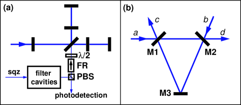
Figure 1: Panel (a) displays the placement of the filter in a squeezed-input interferometer. Panel (b) shows the single filter configuration, where $a$ is the beam to be filtered, $b$ is unsqueezed vacuum, $c$ is the filtered beam and $d$ is the transmitted beam.

The field incident on the the cavity comprises a carrier at frequency, $\omega_{0}$, and sidebands at frequencies, $\omega_{0}\pm\Omega$. When the cavity is resonant with the carrier frequency, $\omega_{0}$, the roundtrip length of the cavity, $l$, is an integer number of carrier half-wavelengths and the $\omega_{0}+\Omega$ component of the incident field will experience a frequency-dependent phase shift, $\Phi=\frac{\Omega l}{c}$ for a single round trip of the cavity. Cavity amplitude reflection and transmission coefficients are then given by

$$\rho\left(\Omega\right) =\displaystyle\frac{c}{a} =\sqrt{R_{1}}-\frac{T_{1}\sqrt{R_{2}\,R_{3}}\,{\rm e}^{2i\Phi}}{1-\sqrt{R_{1}\,R_{2}\,R_{3}}\,{\rm e}^{2i\Phi}},$$ (2)

$$\tau\left(\Omega\right) =\displaystyle\frac{d}{a} =\frac{\sqrt{T_{1}\,T_{2}}\,{\rm e}^{i\Phi}}{1-\sqrt{R_{1}\,R_{2}\,R_{3}}\,{\rm e}^{2i\Phi}}.$$ (3)

To make the cavity act as a high-pass filter for the reflected light at frequency $\Omega$ (relative to the carrier frequency, $\omega_{0}$), a cavity with no reflected light at $\Omega=0$ is desired, so we require that $\rho(0)=0$. We constrain the values of $R_{1}$ and $R_{2}\,R_{3}$ at a fixed value of $A_{1}$ by choosing a value for the half-linewidth of the cavity

$$\gamma_{f} \equiv \frac{c}{4l}(1-R_{1}\,R_{2}\,R_{3}),$$ (4)

$$R_{1} = \sqrt{1-\frac{4l\gamma_{f}}{c}}\left(1-A_{1}\right),$$ (5)

$$R_{2}\,R_{3} = \displaystyle\frac{\sqrt{1-\frac{4l\gamma_{f}}{c}}}{\left(1-A_{1}\right)},$$ (6)

resulting in a reflected beam of the form

$$\rho\left(\Omega\right)=\frac{\sqrt{R}(1-{\rm e}^{2i\Phi})}{1-\sqrt{1-\frac{4l\gamma_{f}}{c}}{\rm e}^{2i\Phi}}\approx\frac{\Omega}{i\gamma_{f}+\Omega}.$$ (7)

Eqn. (7) shows that the performance of the cavity depends only on its linewidth. $R_{2}\,R_{3}$ must be less than $1-A_{2}-A_{3}\approx 1-2A_{1}$, which requires $A_{1}<\frac{2l\gamma_{f}}{3c}$. The finesse of the cavity is $\mathcal{F}=\frac{\pi c}{2l\gamma}$.

III Filtered squeezed states

Since the cavity is not detuned from resonance and there is no rotation of the quadratures, it is straightforward to extend this result to the Caves-Schumaker two-photon formalism CavesSchumaker ; SchumakerCaves . Refering to Fig. 1 (b), $a$ and $b$ are the (complex) amplitudes of fields at sideband frequency, $\Omega$, incident on mirror M1 and M2, respectively. The field reflected from the cavity, $c$, has the form

$$c_{i}=\rho a_{i}+\tau b_{i}+\sqrt{1-|\rho|^{2}-|\tau|^{2}}\,v_{i}\,,$$ (8)

where $i=1,\,2$ and the $v_{i}$ are the quadrature field amplitudes of the unsqueezed vacuum that leaks in due to the losses in the cavity. In the case where the light incident on M2 is also unsqueezed vacuum , the reflected field takes the form

$$c_{i}=\rho a_{i}+\sqrt{1-|\rho|^{2}}\,v_{i}.$$ (9)

Now suppose squeezed vacuum is incident on the cavity, i.e. $a$ is squeezed. Since $\rho(\Omega)$ has the response of a high pass filter, we see from Eqn. (9) that at low frequencies where $\rho(\Omega<\gamma_{f})\sim 0$, the second term dominates and the filter output field, $c$, is in an ordinary vacuum state given by $v$, while at high frequencies where $(1-|\rho|^{2})\sim 0$, the output field contains primarily the squeezed input vacuum, $a$.

The reflected beam is, in general, not a pure squeezed state . Two parameters characterize the effects of the cavity on the squeezed state: the attenuation factor, $\alpha$, and the vacuum leakage, $\beta$. The attenuation factor measures the effect on the anti-squeezed quadrature, while the vacuum leakage measures the effect on the squeezed quadrature by measuring the vacuum noise that enters the beam. Defining $x=\Omega/\gamma_{f}$, we find

$$\alpha= |\rho|^{2} \approx\frac{x^{2}}{1+x^{2}},$$ (10)

$$\beta= 1-|\rho|^{2} \approx\frac{1}{1+x^{2}},$$ (11)

$$\alpha+\beta= 1.$$ (12)

We define the corner frequency, $\xi=x_{1/2}\gamma_{f}$, of the filter to be the frequency at which $\alpha=\beta=\frac{1}{2}$, which gives $x_{1/2}\approx 1$. The parameters $\alpha$ and $\beta$ as a function of (normalized) frequency are plotted as the solid curves in Fig. 2. Discussion of multiple filters, also shown in Fig. 2, is deferred to Section VI.

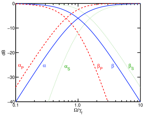
Figure 2: A plot of the attenuation, $\alpha$, and maximum possible squeezing, $\beta$ for a single (blue, solid), series (red, dashed) and parallel (green, dotted) filter. The subscripts $S$ and $P$ refer to series and parallel filters, respectively; these filter configurations are described in Section VI. The series filter increases the effective corner frequency and the attenuation factor, while the parallel filter decreases the effective corner frequency but increases the maximum squeezing.

IV Application to gravitational-wave interferometers

IV.1 Conventional interferometer

It is instructive to study the performance of the amplitude filter cavity with a conventional GW interferometer operated at the optimum power required to reach the standard quantum limit at $\Omega=\gamma$ KLMTV01 . Here $\gamma$ is the linewidth of the arm cavities of the interferometer, distinct from $\gamma_{f}$, which is the linewidth of the filter cavity. Though $\gamma$ may be adjusted to optimize the detector performance under certain circumstances, we restrict ourselves to $\gamma=2\pi\times 100{\rm~{}Hz}$.

A phase-squeezed vacuum beam is filtered by the cavity and then injected into the otherwise unused output port of the interferometer, as shown in Fig. 1 (a). To maintain the same input/output relations as developed in Ref. KLMTV01 , the interferometer input (cavity output) beam is given in the form 

$$a_{1}^{\prime} = \sqrt{\alpha}\,{\rm e}^{R}a_{1}+\sqrt{\beta}\,v_{1}$$ (13)

$$a_{2}^{\prime} = \sqrt{\alpha}\,{\rm e}^{-R}a_{2}+\sqrt{\beta}\,v_{2}.$$ (14)

For an interferometer with arm lengths, $L$, mirror masses, $m$, and injection squeeze factor, $R$, this leads to the noise spectral density

$$S_{h}=\frac{h_{SQL}^{2}}{2\kappa}\left[\alpha\left({\rm e}^{-2R}+\kappa^{2}{\rm e}^{2R}\right)+\beta\left(1+\kappa^{2}\right)\right],$$ (15)

where

$$h_{SQL}\equiv\displaystyle\sqrt{\frac{8\hbar}{m\,\Omega^{2}\,L^{2}}}$$ (16)

is the noise spectral density of the dimensionless gravitational-wave strain at the standard quantum limit for an interferometer with uncorrelated shot noise and radiation-pressure noise, and

$$\kappa=\displaystyle\frac{2\left(I_{0}/I_{SQL}\right)\,\gamma^{4}}{\Omega^{2}\left(\gamma^{2}+\Omega^{2}\right)}$$ (17)

is the effective coupling constant that relates the output signal to the motion of the interferometer mirrors KLMTV01 .

In Fig. 3, we plot the noise spectral densities for a conventional interferometer with squeezed input parameter ${\rm e}^{-2\,R}=0.1$, using different filter cavity configurations. The unfiltered squeezed input gives significantly higher noise at $\Omega\lesssim\gamma$. When the squeezed input is filtered by a single filter, there is a frequency band $\Omega/\gamma\gtrsim 1.5$ in which the sensitivity is worse than the the unfiltered squeezed case, and a corresponding range $\Omega/\gamma\lesssim 1$ in which the sensitivity is worse than the unsqueezed case. We refer to this band around $\Omega/\gamma\sim 1$ as the “transition region”; it is a consequence of the frequency response of the filter. In Section VI we examine some methods to reduce the frequency extent of this transition region such that the low-frequency noise of the squeezed input interferometer approaches that of an interferometer with no squeezing, while preserving the noise reduction at high frequencies.

It is also possible to define a critical frequency above which squeezing is desirable, and below which it is deleterious . Inserting $\alpha+\beta=1$ into eqn. (15) for $S_{h}$, we get

$$S_{h}=\frac{h_{SQL}^{2}}{2\kappa}\left\{\alpha\left[\left({\rm e}^{2R}-1\right)\,\kappa^{2}-\left(1-{\rm e}^{-2R}\right)\right]+\left(1+\kappa^{2}\right)\right\}.$$ (18)

The coefficient of the term in $\alpha$ switches sign at the critical frequency, $\Omega/\gamma=1.44$, which corresponds to the frequency at which the curves in Fig. 3 cross. Since $\beta=0$ and $\alpha=1$ when no filtering is applied, we always have $\alpha<1$ in the filtered case. More generally then, the noise for the unfiltered case is better at frequencies higher than the critical frequency (where $\kappa$ is small), and worse at frequencies below the critical frequency. Moreover, at the critical frequency, the coefficient of $\alpha$ in eqn. (18) is zero and the value of $\alpha$ does not matter. This also explains why the curves for a variety of filter configurations in Fig. 4 all cross at a single frequency. It will become evident in Section V, however, that in optimizing the filter performance using astrophysical criteria, the critical frequency does not play a significant role.

IV.2 Signal-recycled interferometer

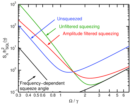
Figure 3: The noise spectral density, normalized by $h_{SQL}$, for a conventional interferometer with (i) no squeezed input (“Unsqueezed”); (ii) squeezed vacuum injected (“Unfiltered Squeezin”); (iii) squeezed input filtered by a filter cavity (“Amplitude filtered squeezing”); and (iv) frequency-dependent squeeze angle (“Frequency-dependent squeeze angle”).

The amplitude filter cavities can also be used in conjunction with a squeezed-input signal-recycled interferometer. The introduction of signal recycling has the effect of mixing the quadratures in the input/output relations of the interferometer. This allows the shot noise and radiation-pressure noise to become correlated, typically producing two resonances BC1 : the lower frequency dip is due to an optical-mechanical coupling and the higher frequency one is a purely optical resonance due to the storage time of the gravitational wave signal in the interferometer. The mixing of the quadratures results in the optimal squeeze angle having a strong frequency dependence compared to the conventional interferometer harms .

The sensitivity curve can be shaped by an appropriate choice of the reflectivity of the signal extraction mirror (SEM) and the detuning of the signal extraction cavity (SEC) pfspie . The noise curves shown in Fig. 4 are for a narrowband signal-recycled interferometer where the detuning of the SEC is chosen to place the optical resonance at 200 Hz. An alternative choice of detuning, where the carrier light with angular frequency $\omega_{l}$ obtains a net phase shift of $\frac{\pi}{2}$ in one pass through the cavity, gives a broadband response. This choice reduces the variation of the optimal squeeze angle with frequency and allows for improvement in the performance over a large frequency range. The broadband interferometer with squeezed input does not, however, benefit from the amplitude filtering unless the squeezed state is not pure. We, therefore, limit our discussion to the narrowband case shown in Fig. 4. Furthermore, we discuss the narrowband signal-recycled interferometer in term of real frequency, in Hz, since the normalization to an arm cavity inverse storage time is not meaningful when the gravtitational-wave signal storage time depends on both the arm cavity and the (detuned) signal extraction cavity.

The performance of the squeezed configuration is comparable to the unsqueezed configuration in the frequency range 10 Hz to 300 Hz, and considerably better between 300 Hz to 10 kHz.

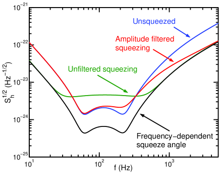
Figure 4: The square root of the noise spectral density for a signal-recycled narrowband Advanced LIGO interferometer with (i) no squeezing (“Unsqueezed”); (ii) squeezed vacuum injected directly into the output port of the beamsplitter (“Unfiltered squeezing”); (iii) squeezed vacuum injected after filtering with an amplitude filter cavity (“Amplitude filtered squeezing”); and (iv) squeezed vacuum injected after filtering to get a ”Frequency-dependent squeeze angle”.

V Filter Performance

To evaluate the performance of these amplitude filters with parameters that can be realized we invoke some simple astrophysical arguments. The amplitude filters are best suited to optimizing the gravitational-wave detector performance at high frequencies without compromising the low-frequency performance as severely as a fixed squeeze angle input with no filtering. To this end, three frequency bands are of interest: (i) high frequencies $\Omega/\gamma\sim 10$ where we expect to carry out searches for GW emission from pulsars, for example; (ii) the minimum in $S_{h}$ around $\Omega/\gamma\sim 1$ which is important for detection of radiation from inspiraling binary systems; and (iii) low frequencies $\Omega/\gamma<1$ which are especially important for detection of a stochastic gravitational-wave background of cosmological origin by correlating the outputs of two spatially separated terrestrial detectors . The performance in each of these frequency bands is characterized by the signal from the targeted source compared with the noise in the detectors. In Table 1, we compare the sensitivity or signal-to-noise ratio (SNR) for pulsars, binary neutron star inspirals and a stochastic background for several amplitude filter cavity configurations with a conventional interferometer with varying input power levels.

Most generally, the square of the signal-to-noise ratio (assuming optimum filtering) is given by thorne300 .

$$\left(\frac{S}{N}\right)^{2}\propto\int_{0}^{+\infty}\frac{|h(f)|^{2}}{S_{h}(f)}\,df$$ (19)

where $h(f)$ is the Fourier transform of the strain signal from the source and $S_{h}(f)$ is the single-sided noise spectral density of the detector.

For periodic sources such as a pulsar at a fixed frequency $\Omega_{s}$, and ignoring any other modulation effects, the SNR can be expressed as

$$\left(\frac{S}{N}\right)_{per}^{2}\propto\int_{0}^{+\infty}\frac{\delta(2\pi\Omega_{s})}{S_{h}(f)}\,df$$ (20)

where $\delta(2\pi\Omega_{s})$ is a Kronecker delta function at $\Omega_{S}$. For our purposes it is convenient to assume $\Omega_{s}=10\,\gamma$, and the signal-to-noise ratio is simply proportional to the inverse of the detector noise spectral density at that frequency.

For the inspiral phase of binary neutron star systems, the Newtonian quadrupole approximation gives $|h(f)|^{2}\propto f^{-7/3}$. We estimate the SNR for inspiraling neutron stars by

$$\left(\frac{S}{N}\right)_{ins}^{2}\propto\int_{10{\rm~{}Hz}}^{+\infty}\frac{1}{f^{7/3}\,S_{h}(f)}\,df$$ (21)

where $S_{h}(f)$ is given by the curves in Figures 3 and 4 and a lower cut-off frequency of $\Omega/\gamma=0.1$ is used to account for seismic noise .

For a stochastic background of cosmological origin, the spectrum of gravitational-waves is given by

$$\left|h(f)\right|^{2}=\frac{3H_{0}^{2}}{10\pi^{2}}f^{-3}E_{gw}(f)$$ (22)

where $H_{0}$ is the present day Hubble expansion rate and $E_{gw}(f)$ is the gravitational-wave energy density per logarithmic frequency, divided by the critical energy density required to close the Universe. Assuming that $E_{gw}(f)={\rm~{}constant~{}}=E_{0}$, and that the waves are isotropic, unpolarized, stationary and Gaussian, we arrive at $\left|h(f)\right|^{2}\propto f^{-3/2}$. Limits on the stochastic background can be set by cross-correlating the outputs of two detectors. To ensure that noise in the detectors is not correlated by shared local effects, we use two widely separated detectors, e.g. detectors at the two LIGO Observatories, which are nearly co-planar and co-aligned but separated by a distance $d_{s}=3001$ km. The cross-correlation depends on an additional quantity, $\eta(f)$, the overlap reduction function, which characterizes the reduction in sensitivity due to the separation time delay and relative orientation of the detectors. For the LIGO detectors in Louisiana and Washington, $\eta(f)$ can be expressed in terms of Bessel functions, $J_{i}\,$: $\eta(f)=-0.124842\,J_{0}\left(2\pi fd_{s}/c\right)-2.90014\,J_{1}\left(2\pi fd_{s}/c\right)+3.00837\,J_{2}\left(2\pi fd_{s}/c\right)$ flanagan , which gives $\eta(f=0{\rm~{}Hz~{}})\approx 0.9$ with a sharp reduction above 50 Hz. The square of the signal-to-noise ratio for the stochastic background obtained by cross-correlating two detectors with noise spectra, $S_{h{\rm 1}}(f)$ and $S_{h{\rm 2}}(f)$, is given by

$$\displaystyle\left(\frac{S}{N}\right)_{sb}^{2} \propto \displaystyle\int_{-\infty}^{+\infty}\frac{\eta(f)^{2}}{f^{6}\,S_{h{\rm 1}}(f)\,S_{h{\rm 2}}(f)}\,df$$ (23)

$$\approx \displaystyle\int_{-\infty}^{+\infty}\frac{\eta(f)^{2}}{f^{6}\,S_{h}^{2}(f)}\,df$$ (24)

The result of Eqn. (24) assumes that the noise spectra of the two detectors are Gaussian, stationary and identical, i.e. $S_{h{\rm 1}}(f)=S_{h{\rm 2}}(f)$, and that optimal filtering was used allen .

Configuration	$\displaystyle\frac{\gamma_{f}}{\gamma}$	Stochastic	NS Inspiral	Periodic
Conventional interferometer	–	$1.00$	$1.00$	$1.00$
Unfiltered fixed-angle squeeze	–	$0.32$	$1.16$	$3.16$
Single filter	$1$	0.89	1.00	3.03
Single filter	$5$	0.99	0.98	1.89
Series filter	$1/\sqrt{2}$	0.98	1.02	3.03
Series filter	$5/\sqrt{2}$	$1.00$	1.01	1.86
Parallel filter	$\sqrt{2}$	0.89	1.09	1.12
Parallel filter	$5\,\sqrt{2}$	$0.99$	0.98	2.24
FD squeeze	–	3.16	3.16	3.16

Table 1: Comparison of performance of a conventional interferometer with different filter configurations using three criteria: the signal-to-noise ratios for detecting (i) a stochastic background of gravitational-waves, (ii) the inspiral phase of a neutron star binary system (NS SNR), and (iii) a periodic source at $\Omega/\gamma=10$ (which is simply the inverse strain spectral density, $1/\sqrt{S_{h}}$, at that frequency). We use the square root of the SNRs defined in Eqns. (20), (21) and (22) with $S_{h}$ corresponding to the various interferometer and filter configurations listed. All SNRs are normalized to that of a conventional interferometer with no squeezing. The series and parallel filter configurations are described in Section VI.

Configuration	$\displaystyle\frac{\gamma_{f}}{100{\rm~{}Hz}}$	NS Inspiral	$\displaystyle\frac{1}{\sqrt{S_{h}}}\left(\frac{\Omega}{2\pi}=1{\rm~{}kHz}\right)$	$\displaystyle\frac{1}{\sqrt{S_{h}}}\left(\frac{\Omega}{2\pi}=10{\rm~{}kHz}\right)$
SR interferometer	–	$1.00$	$1.00$	$1.00$
Unfiltered fixed-angle squeeze	–	$0.654$	$3.16$	$3.08$
Single filter	$3$	$0.854$	$2.39$	$3.07$
Single filter	$5$	$0.924$	$1.89$	$3.05$
Single filter	$10$	$0.974$	$1.35$	$2.96$
FD squeeze	–	3.16	3.16	$3.16$

Table 2: Comparison of performance of a narrowband signal-recycled interferometer with different filter configurations using two criteria: The signal-to-noise ratio for (i) inspiraling neutron star binaries (NS Inspiral), and (ii) periodic sources radiating at 1 kHz and 10 kHz, respectively. All SNRs are normalized to that of a signal-recycled interferometer with no squeezing.

Table 1 and Fig. 3 show that the best overall configuration is no doubt the frequency-dependent squeeze angle. Assuming that the interferometers are operated at the maximum power possible, then the only way to improve the high frequency noise is to use squeezing. If no filtering is used, the binary inspiral SNR is significantly reduced. If an amplitude filter is used in conjunction with the squeezed input, a moderate reduction in binary inspiral SNR is traded off against the benefits of squeezing at higher frequencies. The choice of bandwidth of the filter influences this trade off. Furthermore, the amplitude filtered squeezing can be used to increase sensitivity to binary inspirals by lowering the power, and using the squeezing to not completely worsen the high frequency noise. In the likely event that the multiple kilometer-scale filter cavities needed to achieve the frequency-dependent squeeze angle are not feasible in the upcoming generation of interferometers, amplitude filters such as the ones we propose are promising candidates for broadband improvement in the detector sensitivity.

To explore the feasibility of these filter cavities further, we give some physical parameters for the amplitude filter cavities. For a conventional interferometer with initial LIGO parameters $\gamma\simeq 2\pi\times 100$ Hz. From Table 1, we see that $\gamma\lesssim\gamma_{f}\lesssim 5\,\gamma$, implying that the filter cavity linewidth is typically equal to, or a few times larger, than the arm cavity linewidth, or $500\,{\rm Hz}\gtrsim\gamma_{f}/(2\pi)\gtrsim 100\,{\rm Hz}$. For a 10 meter long filter cavity, this would correspond to a finesse of 15000 to 75000, or average losses of 70 to 14 parts-per-million per mirror. If the filter cavities can be made longer (upto $\sim 30$ m is feasible in the output train of LIGO), the limit on the mirror losses can be accordingly relaxed.

For completeness we evaluate the performance of a narrowband signal-recycled interferometer as well. As with the conventional interferometer, the narrowband signal-recycled configuration of Fig. 4 and Table 2 benefits at all frequencies from squeezed input with a frequency-dependent squeeze angle. We intentionally use a narrowband configuration to highlight the differences between it and the conventional interferometer. It is evident from Fig. 4 that for the narrowband signal-recycled configuration, the amplitude filter gives significant improvement for detection of neutron star binary inspirals (the SNR is most sensitive to detector noise in the minimum between 40 and 400 Hz), but would certainly deteriorate the detector performance for the stochastic background (the overlap reduction function strongly favors frequencies below 50 Hz). In Table 2 it is interesting to note that the filter cavity can provide substantial benefit at high frequencies even with considerably higher resonance bandwidths, e.g. 1 kHz.

VI Extension to multiple filters

In this section we explore methods to reduce the frequency extent of the transition region between the reduced noise at high frequencies (due to squeezing) and the increased noise at low frequencies, that can be made to approach the noise level of an interferometer with no squeezing.

VI.1 Series filters

The most straightforward way to reduce the transition region is to connect two filters in series, as shown in Fig. 5(a). Extending Eqns. 7, 11 and 12, we find

$$\alpha_{S}= |\rho|^{4} \approx\frac{x^{4}}{x^{4}+2x^{2}+1},$$ (25)

$$\beta_{S}= 1-|\rho|^{4} \approx\frac{2x^{2}+1}{x^{4}+2x^{2}+1},$$ (26)

$$x_{1/2}\approx \left(\sqrt{2}+1\right)^{\frac{1}{2}}.$$ (27)

Comparing the solid curves with the dotted curves in Fig. 2, we see that the addition of the second filter has the effect of increasing the attenuation factor, while shifting the vacuum leakage by a factor of $\sqrt{2}$ in frequency at frequencies $\Omega\gtrsim\gamma$. By reducing the linewidth of both filters by a factor $\sqrt{2}$, we obtain nearly the same vacuum leakage along with an increased attenuation factor, thereby reducing the size of the transition region. For ease of comparison, in the ”series filter” curve of Fig. 6 the linewidth of each filter cavity is reduced by $\sqrt{2}$ compared to an equivalent single filter. We also note that further gains could be made by double-passing the input squeezed light through each filter, or, alternatively, reducing the number of filters required, and hence reducing the complexity.

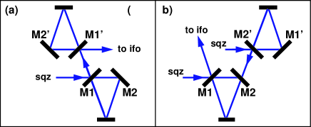
Figure 5: Panel (a) shows the series filter, in which the input beam passes through two filters. Panel (b) shows the parallel filter, in which a filtered beam is injected instead of vacuum.

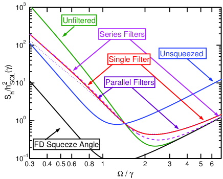
Figure 6: The square root of the noise spectral density is shown for a conventional interferometer with (i) no squeezed input (”Unsqueezed”), (ii) Squeezed vacuum injected (”Unfiltered”); Squeezed input filtered by (iii) a single filter cavity (”Single Filter”), (iv) series filter cavities (”Series Filter”), (v) parallel filter cavities (”Parallel Filter”); and (vi) frequency-dependent squeeze angle (”FD Squeeze Angle”).

VI.2 Parallel filters

To decrease the vacuum leakage, we inject the filtered beam from one filter into the input port of another filter, as shown in Fig. 5 (b). We assume that the input light in each filter is squeezed in the same quadrature. We also assume that the filters are lossless for simplicity. The output from the combined filters is

$$c_{i}=\rho\left(a_{i}+\tau b_{i}\right)+\tau^{2}v_{i}$$ (28)

where $a_{i}$ is the field injected in the first filter, and $b_{i}$ is the field injected into the second filter. Using the relation that $|\rho|^{2}+|\tau|^{2}=1$ for a lossless filter, we find that

$$\alpha_{P}= |\rho|^{2}\left(2-|\rho|^{2}\right) \approx\frac{x^{4}+2x^{2}}{x^{4}+2x^{2}+1},$$ (29)

$$\beta_{P}= \left(1-|\rho|^{2}\right)^{2} \approx\frac{1}{x^{4}+2x^{2}+1},$$ (30)

$$x_{1/2}\approx \left(\sqrt{2}-1\right)^{\frac{1}{2}}.$$ (31)

As shown in the dashed curves of Fig. 2, the parallel filter has the effect of decreasing the vacuum leakage, while shifting the attenuation factor by a factor of $\sqrt{2}$ in frequency at frequencies $\Omega\lesssim\gamma$. By increasing the linewidth of both filters by a factor $\sqrt{2}$, we can obtain nearly the same attenuation factor along with reduced vacuum leakage, once again reducing the size of the transition region.

VI.3 Filter Performance

It is instructive to evaluate the sensitivity of the interferometer with squeezed input filtered by the multiple cavity configurations. For conciseness, we apply multiple filters only to the conventional interferometer described in Section IV.1. The performance measures are listed in the series and parallel filter sections of Table 1, where we apply the same criteria as those described in Section V, namely, the signal-to-noise ratios for detecting gravitational radiation from (i) a stochastic background using widely separated detectors, (ii) an inspiraling neutron star binary system, and (iii) a perfectly periodic source at $\Omega/\gamma=10$.

VII Conclusion

Recognizing the operational complexity of using kilometer-scale filter cavities in conjunction with a squeezed input in long-baseline gravitational-wave interferometers, we have proposed an alternative type of filter cavity that acts as a high-pass filter for the squeeze amplitude. We evaluate the performance of these amplitude filters with parameters that can be realized and find them to be effective in improving the high-frequency performance of a squeezed input gravitational-wave detector without drastically compromising the low-frequency sensitivity. From Table. 1, we see that that significant improvements can be achieved with the amplitude-filtered squeezed input interferometer compared with an interferometer with no squeezing, or with a frequency-independent squeezed-input interferometer, depending on the target astrophysical source and the interferometer and filter parameters. The amplitude filters do not give the broadband improvement afforded by the (multiple) kilometer-scale filter cavities that give a frequency-dependent squeeze angle, but they are an attractive alternative since they are a few meters in length and require finesses well under $10^{5}$, making them more feasible in the output train of gravitational-wave detectors. Moreover, the amplitude filters can suppress noise in excess of the anti-squeezed quantum-limited noise. We also point out that some of the broadband benefit afforded by the frequency-dependent squeeze angle – or any other filtering scheme – is likely to be compromised by other noise sources, e.g., thermal noise, which were not considered in this work.

- (1) A. Abramovici et al., Science 256, 325 (1992).
- (2) C. M. Caves, Phys. Rev. Lett. 45, 75 (1980).
- (3) C. M. Caves, Phys. Rev. D 23, p. 1693 (1981).
- (4) W. G. Unruh, in Quantum Optics, Experimental Gravitation, and Measurement Theory, eds. P. Meystre and M. O. Scully (Plenum, 1982), p. 647.
- (5) H. J. Kimble, Yu. Levin, A. B. Matsko, K. S. Thorne and S. P. Vyatchanin, Phys. Rev. D 65, 022002 (2002).
- (6) J. Harms, Y. Chen, S. Chelkowski, A. Franzen, H. Vahlbruch, K. Danzmann, R. Schnabel, “Squeezed-input, optical-spring, signal-recycled gravitational-wave detectors,” gr-qc/0303066.
- (7) T. Corbitt and N. Mavalvala, Proceedings of SPIE, Fluctuations and Noise in Photonics and Quantum Optics, Santa Fe, NM, 5111 (2003), p. 23. gr-qc/0306055.
- (8) A. Buonanno and Y. Chen, “Improving the sensitivity to gravitational-wave sources by modifying the input-output optics of advanced interferometers,” gr-qc/0310026.
- (9) C. M. Caves and B. L. Schumaker, Phys. Rev. A 31, 3068 (1985).
- (10) B. S. Schumaker and C. M. Caves, Phys. Rev. A 31, 3093 (1985).
- (11) P. Fritschel, “Second generation instruments for the Laser Interferometer Gravitational-wave Observatory (LIGO),” in Gravitational Wave Detection, Proc. SPIE 4856-39, p. 282, 2002. gr-qc/0308090.
- (12) A. Buonanno and Y. Chen, “Quantum noise in second-generation signal-recycled laser interferometric gravitational wave detectors,” Phys. Rev. D 64, 042006 (2001).
- (13) K. S. Thorne, in 300 Years of Gravitation, edited by S. W. Hawking and W. Israel (Cambridge Universtiy Press, Cambridge, 1987), p. 369 and p. 380.
- (14) É. É. Flanagan, “Sensitivity of the laser interferometer gravitational wave observatory (LIGO) to a stochastic background, and its dependence on the detector orientations,” Phys. Rev. D 48, 389 (1993).
- (15) B. Allen and J.D. Romano, “Detecting a stochastic background of gravitational radiation: Signal processing strategies and sensitivities,” Phys. Rev. D 59, 102001 (1999).