Equilibrium Configurations of Homogeneous Fluids in General Relativity

Abstract

By means of a highly accurate, multi-domain, pseudo-spectral method, we investigate the solution space of uniformly rotating, homogeneous and axisymmetric relativistic fluid bodies. It turns out that this space can be divided up into classes of solutions. In this paper, we present two new classes including relativistic core-ring and two-ring solutions. Combining our knowledge of the first four classes with post-Newtonian results and the Newtonian portion of the first ten classes, we present the qualitative behaviour of the entire relativistic solution space. The Newtonian disc limit can only be reached by going through infinitely many of the aforementioned classes. Only once this limiting process has been consummated, can one proceed again into the relativistic regime and arrive at the analytically known relativistic disc of dust.

1 Introduction

Self-gravitating bodies of constant density have always played a central role in the physics of gravitation. Contributions that have been most significant to the aspects of this subject that will be relevant to this paper can be divided into (1) work done within Newton’s theory of gravitation: Maclaurin (1801), Poincaré (1885), Dyson (1892, 1893), Lichtenstein (1933), Wong (1974) and Eriguchi & Sugimoto (1981) and (2) work done within Einstein’s theory of gravitation: Schwarzschild (1916), Chandrasekhar (1967), Bardeen (1971), Butterworth & Ipser (1976) and Gondek-Rosińska & Gourgoulhon (2002). Despite this great investment of effort, it has not yet been possible to explore the whole spectrum of Newtonian, let alone relativistic solutions, even if one restricts oneself to axial symmetry and stationarity. Using sophisticated computer programs, we believe that a great step can be taken toward painting the complete relativistic picture of uniformly rotating, homogeneous and axisymmetric bodies. However, because of the many intricate details in this picture, particularly in the vicinity of limiting configurations, it is necessary to use a computer program robust enough to be able to render such limiting configurations and accurate enough to be able to distinguish between neighbouring solutions of Einstein’s equations. For our investigations of homogeneous fluids, we used a code based on multi-domain pseudo-spectral methods (Ansorg et al., 2002, 2003a), which satisfies these requirements. For a comparison with other codes, see Stergioulas (2003).

It is our intention in this paper to present the relativistic picture in its entirety by describing those parts of it that we have studied explicitly and augmenting them with conjectures as to the rest. With this in mind, we focus our attention neither on the numerical methods nor primarily on properties of individual configurations (as in Ansorg et al. 2003b; Schöbel & Ansorg 2003), but instead emphasize the interrelations between various configurations and portray the solution space as a whole. As an interesting example of the newly explored configurations, we present the shape and various physical parameters of a core-ring solution.

The picture that emerges for relativistic homogeneous fluids contains familiar demarcations, which we can use to orient ourselves. It contains, for example, three analytically known solutions: the (inner and outer) Schwarzschild solution (Schwarzschild, 1916), the relativistic disc of dust solution (Bardeen & Wagoner, 1971; Neugebauer & Meinel, 1995, 2003) as well as the Maclaurin solution (Maclaurin, 1801) as one of its Newtonian limits. This last solution will be a particularly useful point of departure for describing the corresponding relativistic picture. It represents homogeneous, rotating fluid spheroids and, but for a scaling factor, depends for given mass density on only one parameter, thereby allowing one to refer to the “Maclaurin sequence”. After introducing some basic equations in Sec. 2 we thus turn our attention to the Maclaurin solution and its post-Newtonian extension in Sec. 3. It turns out that not all relativistic configurations are connected to each other in a continuous way, and it will be useful to introduce the notion of a class of solutions. A given class will be defined to include all configurations of strictly positive mass that are connected continuously to each other. In Sec. 4 we review the characteristics of the “first” three classes in detail and provide an overview of the remaining classes. We close with a discussion of the limitations of numerical methods and some thoughts on the completeness of the relativistic picture painted in this paper.

2 Einstein’s Field Equations and their Numerical Solution

Using Lewis-Papapetrou coordinates, the line element for a stationary, axially symmetric spacetime corresponding to a rigidly rotating perfect fluid configuration can be written in the form

$$ds^{2}=e^{2\alpha}(d\varrho^{2}+d\zeta^{2})+W^{2}e^{-2\nu}(d\varphi-\omega\,dt)^{2}-e^{2\nu}\,dt^{2},$$

where the metric functions $\alpha$, $W$, $\nu$ and $\omega$ are functions of $\varrho$ and $\zeta$ alone. The boundary of a fluid configuration rotating with the angular velocity $\Omega$ obeys the equation

$$e^{2\nu}-W^{2}(\omega-\Omega)^{2}e^{-2\nu}=\text{const.}=\left(1+Z_{0}\right)^{-2},$$

where $Z_{0}$ is the relative redshift observed at infinity of a photon emitted with zero angular momentum from the configuration’s surface. Together with regularity requirements along the axis of rotation, $\varrho=0$, and the asymptotic behaviour, the boundary equation including transition conditions and the field equations themselves form a complete set of equations to be solved (see e.g. Butterworth & Ipser 1976). In this paper we choose natural units in which the gravitational constant $G$ and the speed of light $c$ are both equal to one.

This set of equations was solved numerically to very high accuracy using a multi-domain pseudo-spectral method. In the algorithm used, the domains are chosen such that the unknown boundary $\zeta=\zeta_{\text{s}}(\varrho)$ of the configuration always coincides with the boundary between two domains, thus avoiding Gibbs’ phenomena. The boundary enters into the equations through coordinate transformations, which map the physical domains onto a square. The metric functions and the boundary are represented by a truncated Chebyshev expansion so that the above mentioned set of equations can be reduced to a set of (non-linear) algebraic equations. Typically, we used between 10 and 30 Chebyshev coefficients per dimension, depending on the properties of the function being represented. The parameters we can set to specify a fluid configuration include a mass-shedding parameter ($\beta$ of Sec. 4.1) and central pressure, which can be set strictly to infinity (through a rescaling), thereby allowing us to study even the boundary configurations to be discussed in this paper with great accuracy. Further details can be found in Ansorg et al. (2003a).

3 The Maclaurin Sequence and its Bifurcation Points

Maclaurin showed that for a spheroid (also called an ellipsoid of rotation) of constant density there is a balance of gravitational, centrifugal and pressure forces, leading to equilibrium in Newtonian theory. For a given mass density, this spheroid can be described entirely by specifying the ratio of polar to equatorial radius,

$$A:=r_{1}/r_{2},$$ (1)

and the focal distance of the ellipse used to generate this ellipsoid of revolution. The focal distance merely provides the scaling of the spheroid and we can use $A\in[0,1]$ to parametrize the whole solution.

Poincaré (1885), Bardeen (1971) and Hachisu & Eriguchi (1984) all studied points of instability along the Maclaurin sequence and the latter three authors were able to show that these correspond to bifurcation points. The bifurcation points that are of particular interest to us here are those marking the onset of the various modes of axially symmetric, secular instability. Values for $A$ at the first few of these can be found in Table 1 and will be denoted by $A_{n}$, ($n=1,2,3,\ldots$).

Table 1: Values for the ratio of polar to equatorial radius of the Maclaurin spheroid at the first six bifurcation points associated with the onset of axially symmetric, secular instability.

Bifurcation points
$A_{1}=0.17126186\ldots$
$A_{2}=0.11160323\ldots$
$A_{3}=0.08274993\ldots$
$A_{4}=0.06574427\ldots$
$A_{5}=0.05453402\ldots$
$A_{6}=0.04658868\ldots$

There are countably infinitely many such bifurcation points with the accumulation point $A=0$. Chandrasekhar (1967) calculated the post-Newtonian corrections to the Maclaurin spheroids and found that they become singular at the bifurcation point $A_{1}$. Bardeen (1971) conjectured that the $n^{\text{th}}$ post-Newtonian approximation to the Maclaurin spheroids becomes singular at each of the first $n$ such bifurcation points – a conjecture which was then proved in Petroff (2003).

Assuming the convergence of the post-Newtonian series, an assumption based on strong evidence especially in the disc limit (see Petroff & Meinel 2001), the singularities then represent impermeable barriers in an appropriate parameter space. These barriers allow us to divide our solution space into “classes” of configurations in the following way: We first divide up the Maclaurin sequence into an infinite number of segments with the above mentioned bifurcation points, $A_{n}$, separating one segment from the next. These segments can be numbered (or named) starting, for example, from $A=1$. We can then identify uniquely any configuration of strictly positive mass with a given segement by requiring that the segment be approachable in a continuous way. All those configurations that have been thus associated with segment $n$ make up class $n$.

As we shall see in the following sections, numerical results lend strong support to the idea that such impermeable barriers as were mentioned above exist and that the definition of a class is thereby justified. In particular, we shall see that it is possible to place ourselves at one of the end-points of a Maclaurin segment and move off the Maclaurin sequence along other well-defined boundaries until we land again on the Maclaurin segment at the second end-point. Neighbouring classes have only this one point as a common boundary.

4 The Relativistic Classes

4.1 Class I: The Generalized Schwarzschild Class

The first class of configurations that will be discussed in this paper was explored extensively in Schöbel & Ansorg (2003). Here we shall give a brief overview of it, paying particular attention to its defining boundaries.

For a given constant mass density, $\mu$, a stationary, axisymmetric, rigidly rotating relativistic fluid depends on two parameters. A limiting configuration, i.e. one that possesses a physical property representing a boundary, is specified by fixing a corresponding parameter, meaning that it depends on only one further parameter. It is therefore possible to refer to a boundary sequence and identify the end-points of this sequence uniquely with respect to the second parameter.

Clearly the static boundary is marked by the specification $A=1$. (Note that we also use the radius ratio as defined in Eq. (1) in the relativistic context, where $r_{1}$ and $r_{2}$ are now coordinate radii.) Static configurations are described by the analytic Schwarzschild solution, which can be parametrized by their central pressure, $p_{\text{c}}$. Starting from the static end of the Maclaurin sequence ($A=1,p_{\text{c}}=0$), let us increase the central pressure until it becomes infinite. This sequence corresponds to a mere point in the lower right corner of Fig. 1 and to the segment from (a) to (b) in the schematic diagram of Fig. 4. Configurations with infinite central pressure are also clearly boundary configurations. We can parametrize these by the normalized angular velocity and follow the sequence from the static limit (where the angular velocity is of course zero) up to its maximal value marked by a mass-shedding limit ((b) to (c) in Fig. 4). Configurations at the mass-shedding limit rotate with an angular velocity equal to that of a test mass rotating at the equator on a circular orbit. They exhibit a cusp at the equatorial rim and are thus easy to identify by the geometry of their surface. We define a mass-shedding parameter $\beta$ as in Ansorg et al. (2003a) by

$$\beta:=-\frac{{r_{2}}}{{r_{1}}^{2}}\lim_{\varrho\to r_{2}}\,\zeta_{\text{s}}\frac{d\zeta_{\text{s}}}{d\varrho},$$

where $\zeta=\zeta_{\text{s}}(\varrho)$ represents the boundary of the configuration (see Section 2). The mass-shedding parameter takes on the value $\beta=0$ in the mass-shedding limit and $\beta=1$ for Maclaurin spheroids. Fixing the value $\beta=0$, we proceed along the mass-shedding sequence by reducing the central pressure until we reach the Newtonian limit $p_{\text{c}}=0$ ((c) to (d)).

We can trace the last part of this sequence in the enlargement in Fig. 1, i.e. follow the red curve as it comes in from the top. This curve crosses the Maclaurin sequence in the parameters plotted there at a value for the radius ratio of $A\approx 0.195$. The two configurations at this cross-over point are however clearly not the same since one is a relativistic star rotating at the mass-shedding limit whereas the other belongs to the Newtonian Maclaurin sequence. In some other parameter diagram these two configurations would correspond to distinct points. This and various other intersections in Fig. 1 are merely a consequence of the fact that the configurations considered in this paper depend on two parameters, but not always in a unique way.

We resume our journey along the boundary curves by following the Newtonian sequence, $A_{1}^{+}$, from (d) to (e) (parametrized again by $p_{\text{c}}=0$ for example) by increasing $\beta$ until we reach the Maclaurin curve at the value $\beta=1$ and find ourselves precisely at the bifurcation point $A=A_{1}$. This Newtonian sequence and indeed all Newtonian sequences bifurcating from the Maclaurin sequence at the first ten $A_{n}$ were studied in Ansorg et al. (2003c) in which a depiction of the shape of the configurations along these sequences was also provided.

Figure 1: The square of the normalized angular velocity versus the ratio of radii for the boundary curves of the first three classes.

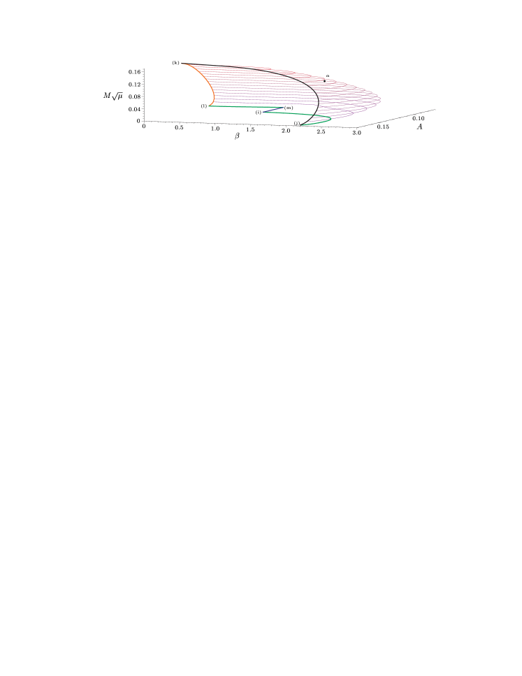
Figure 2: A three-dimensional parameter diagram depicting all of class III. Lines of constant $M\sqrt{\mu}$ beginning with the Newtonian limit $M\sqrt{\mu}=0$ (green and blue curves) are drawn in steps of 0.01. The colour coding of the boundary sequences corresponds to that of Fig. 1.

Except for the Schwarzschild solution itself, we consider all the boundaries in the classes to be open, i.e. the limiting sequences themselves are not considered to belong to a solution class. In the case of the Newtonian limit or the limit of configurations with infinite central pressure, it seems appropriate to exclude such configurations from the physically permissable solutions. In the case of the mass-shedding limit or the two-body limit that will arise in later classes, this choice is a mere matter of convention. The extreme Kerr Black Hole, which will present itself in the next section, is also taken to be an open boundary.

Having circumscribed the generalized Schwarzschild class by specifying its boundary configurations, it is possible to discuss those configurations making up this class. Amongst the most interesting properties of this first class is that there is an upper limit on the attainable mass, which is much higher than that known from the static solution. The maximal gravitational mass $M\approx 0.19435/\sqrt{\mu}$ is roughly 34% greater than for the corresponding non-rotating configuration and is reached at (c).

4.2 Class II: The Generalized Dyson Ring Class

A portion of the generalized Dyson ring class was explored in Ansorg et al. (2003b). Here we extend that work and define the entire class by navigating its boundaries as with class I. We begin by placing ourselves on the Maclaurin curve at the point $A=A_{1}$ and proceeding along the sequence $A_{1}^{-}$ by decreasing the value of $A$ for $M\sqrt{\mu}=0$. It turns out that configurations along this sequence pinch together in the centre ($A=0$), marking the transition from a spheroidal to a toroidal topology. This behaviour was predicted by Bardeen (1971), who also correctly surmised that ring configurations are connected to the Maclaurin sequence via the bifurcation point $A_{1}$. Wong (1974) as well as Eriguchi & Sugimoto (1981) studied such configurations and their connection to the Maclaurin sequence, aspects of which were clarified in Ansorg et al. (2003c).

If we define $A$ for toroidal topologies to be the negative ratio of the inner to outer coordinate radius of the ring, i.e.

$$A:=\frac{r_{1}}{r_{2}}\left\{\begin{array}[c]{ll}\begin{array}[]{lll}r_{1}&=&\text{polar radius}\\ r_{2}&=&\text{equatorial radius}\end{array}&\text{spheroidal}\\ \\ \begin{array}[]{lll}-r_{1}&=&\text{inner radius}\\ r_{2}&=&\text{outer radius}\end{array}&\text{toroidal}\end{array}\right.$$

then we can continue to decrease its value until we finally arrive at $A=-1$. This limit, about which Dyson expanded his ring solution (Dyson, 1892, 1893), is problematic however, since the “corotating Newtonian surface potential” tends to minus infinity if the Newtonian mass and the radius $r_{2}$ are chosen to be strictly positive and finite. The open circle at (f) in Figs 1 and 4 indicates the subtle and interesting jump to the extreme Kerr Black Hole limit ($Z_{0}\to\infty$).

Although the horizon of the extreme Kerr Black Hole viewed from the “outside” world is a mere point at the origin of the coordinate system used here, there exists an “inner” world (if the limit is taken in rescaled coordinates, see Ansorg et al. 2003b; Meinel 2002) in which we can increase the value of $A$ until we come to a mass-shedding limit ((f) to (g) in Fig. 4). Following the mass-shedding sequence by decreasing the relative redshift, $Z_{0}$, we cross back over to spheroidal topologies and arrive at the Newtonian mass-shedding configuration for a redshift of zero ((g) to (h)). Following the Newtonian sequence $A_{2}^{+}$ by increasing the value of the mass-shedding parameter, $\beta$, we arrive at the bifurcation point $A_{2}$ of the Maclaurin sequence and have completely circumscribed the generalized Dyson-Ring class ((h) to (i)).

The configurations in this class, in contrast to those of the generalized Schwarzschild class, contain no upper bound for the mass. This surprising fact would only be of astrophysical relevance if ring configurations turned out to be stable.

Another salient feature of this class is that a continuous transition to an (extreme Kerr) Black Hole is possible. This can be compared to the first class for which configurations reached the boundary of infinite central pressure for finite values of the redshift, which has a global maximum of $Z_{0}\approx 7.37825$ in the generalized Schwarzschild class. Note that the extreme Kerr Black Hole is the only candidate for a Black Hole limit of rotating fluid bodies in equilibrium (Meinel, 2004).

4.3 Class III: The First Generalized Core-Ring Class

In this section, we turn our attention to the hitherto unexplored class III and locate its boundaries, depict it in a three-dimensional parameter space and provide a representative example of one of its configurations. Having arrived at $A=A_{2}$ from class II by increasing the value of $A$ (cf. Fig. 1), we proceed into the third class along the Newtonian sequence $A_{2}^{-}$ by placing ourselves at $A=A_{2}$ and increasing the value of this ratio further. The configurations take on a central bulge shape, but begin to pinch in toward the outer edge. Finally the indentation pinches together yielding a ring just barely in contact with a central core corresponding to the path from (i) to (j) in Fig. 4 (see Fig. 7 in Ansorg et al. 2003c). Although it would be possible to consider the separation of core and ring, we are not interested here in studying a many-body problem and restrict our attention to single, homogeneous bodies. Thus this “pinching together” marks an end-point of the Newtonian sequence. We can follow the sequence of configurations on the verge of forming a two-body system by allowing the mass to increase. This sequence ends in a mass-shedding limit for the configuration with a global maximum for $M\sqrt{\mu}\approx 0.16$ in this class ((j) to (k) in Fig. 4). Placing ourselves on the mass-shedding sequence, we can allow the mass to decrease until we reach the Newtonian limit ((k) to (l)). From here, the Newtonian sequence can be followed to the point $A=A_{3}$ by increasing the parameter $\beta$ ((l) to (m)).

As was discussed in Sec. 4.1, two parameters do not necessarily suffice to describe a configuration uniquely. By adding a third dimension, one can resolve such ambiguities. In Fig. 2, a plot of the $A$, $\beta$ and $M\sqrt{\mu}$ values for the configurations of Class III can be found. In this plot, a given point on the two-dimensional surface in the three-dimensional parameter space refers only to a single configuration. A projection of the boundary curves onto the $A$-$\beta$ plane would yield a picture of similar complexity to the depiction of class III in Fig. 1.

An example of various physical parameters for a configuration with the prescribed values $A=0.1$, $M\sqrt{\mu}=0.1$ can be found in Table 2. The shape of the boundary of this configuration in meridional cross-section is shown in Fig. 3.

Table 2: Values for dimensionless physical quantities for an exemplary configuration in Class III with increasing order, $m$ (see Ansorg et al. 2003a), of the numerical approximation. The quantities not yet referred to in this paper, $M_{0}$, $J$ and $R_{\text{circ}}$ are baryonic mass, angular momentum and circumferential radius respectively. The position of this configuration in Figs 1 and 2 is marked by the letter $\alpha$.

	$m=20$	$m=30$	$m=40$
$A$	0.1	0.1	0.1
$M\sqrt{\mu}$	0.1	0.1	0.1
$M_{0}\sqrt{\mu}$	0.1093062	0.10930610	0.109306099
$J\mu$	0.01483899	0.014838966	0.0148389661
$\Omega/\sqrt{\mu}$	0.8627113	0.86271067	0.862710640
$R_{\text{circ}}\sqrt{\mu}$	0.5843826	0.58437986	0.584379882
$Z_{0}$	0.4921657	0.49216554	0.492165525

Figure 3: The meridional cross-section of the boundary of the Class III configuration described in Table 2.

4.4 The Further Classes

As one moves to higher and higher classes, the configurations tend to grow more disc-like. The distance from the Maclaurin curve in the parameters of Fig. 1 grows small although the shapes of the configurations deviate significantly from a spheroid. We term the odd classes, beginning with the third, “core-ring” classes because the configurations on the verge of forming a two-body system contain a central body with a surrounding ring. The central body will itself grow flat in shape and corrugated in appearance as one moves to higher classes. Beginning with the fourth class, the even ones, on the other hand, tend to grow concave at the centre as they “emerge” from the bifurcation points. They then pinch together at the centre and proceed into the toroidal region in which $A$ is negative. Here too, the ring configurations grow flat and corrugated as one moves to higher classes. The corrugations become more pronounced until finally one of them (presumably the outermost) pinches together, whence the name “two-ring” classes for such configurations. The number of corrugations of the Newtonian sequences is described in Ansorg et al. (2003c). There it was shown at least up to $A_{10}$ that the two Newtonian sequences bifurcating from each $A_{n}$ end in a mass-shedding limit and a two-body configuration respectively. We assume that this holds for all the bifurcation points. Emanating from the two bifurcation points associated with a given class are two Newtonian sequences, the one ending in a mass-shedding limit and the other in a two-body system. Insofar as the Black Hole limit and that of infinite central pressure are precluded from the higher classes (as indicated by our numerical investigations), the two end-points of the Newtonian sequences are connected by a mass-shedding and a two-body sequence. The point at which these two configurations meet most likely marks the configuration with the greatest mass for that class.

In order to arrive at this picture for the higher classes, we made use of the first ten Newtonian bifurcation sequences presented in Ansorg et al. (2003c) and the post-Newtonian behaviour in order to make a conjecture, which could then be verified by studying two new classes (III and IV). The properties of the remaining classes could then be extrapolated and, as such, cannot be considered absolutely certain, but rest on firm ground.

Figure 4: A schematic portrayal of the classes and their boundaries. A depiction of the surface of configurations in meridional cross-section is provided for configurations at the intersection point of two boundary sequences (except for the point (f), see Sec. 4.2). In addition, various surfaces are shown to help illustrate the transition from one corner to the next. Whenever ergo-regions arise, they are depicted by dashed lines (hence the dot in the centre of the configuration located at (b)).

In Fig. 4, the classes are depicted schematically. As in this depiction, two neighbouring classes have only the bifurcation point along the Maclaurin sequence in common. The first two classes are atypical in that the first contains the static boundary sequence and one with infinite central pressure and the second contains a sequence of infinite redshift (extreme Kerr Black Hole sequence). Furthermore, these are the only two classes in which we found ergo-regions. Our investigations show that they are always toroidal in topology and “begin” to appear within the fluid configuration. A more detailed discussion of the ergo-regions can be found in Ansorg et al. (2003a, b).

The definition of the classes given in Section 3 relies on the fact that neighbouring classes have only the bifurcation point along the Maclaurin sequence $A_{n}$ as a common boundary. As was already mentioned, the post-Newtonian approximation strongly suggests that any sequence of constant, strictly positive mass, parametrized by $\beta$ and $A$ for example, will be deflected away from the singular point $r_{1}/r_{2}=A_{n}$ and “back into” the original class. This is exactly what is observed numerically.

Figure 5: The relationship of $\beta$ to $A$ for sequences of constant mass in the vicinity of the bifurcation point associated with $A_{1}$ (the point (e), cf. Fig. 4). The solid line represents configurations with $M\sqrt{\mu}=10^{-4}$, the dashed line with $M\sqrt{\mu}=10^{-5}$ and the dotted line with $M\sqrt{\mu}=10^{-6}$. The thin horizontal line represents the Maclaurin sequence and the thin line crossing it is made up of the Newtonian bifurcation sequences $A_{1}^{+}$ and $A_{1}^{-}$ (see Fig. 4). Note the gap between the sequences of class I and class II.

In Fig. 5, $\beta$ versus $A$ values are plotted for sequences of constant mass. Numerical investigations show that sequences belonging to different classes are completely disjoint although the gap in the vicinity of a given $A_{n}$ grows small for decreasing mass and approaches the point $(A_{n},1)$. This feature, which was already conjectured by Bardeen (1971), can be seen distinctly in the figure around $A_{1}$. Such a gap was observed numerically around $A_{2}$ and $A_{3}$ as well. A comparison with Fig. 2 shows why the curve $M\sqrt{\mu}=0.01$ of that plot deviates so markedly from the Newtonian boundary curves. If one were to plot such contour lines for increasingly diminishing values of $M\sqrt{\mu}$, the tendency to approach the Newtonian limit would be evident.

5 Discussion

Numerical evidence suggests that as one proceeds to flatter configurations (higher classes), the departure from the Newtonian sequence grows small. This is reflected in the fact that boundaries associated with highly relativistic attributes such as infinite central pressure or the transition to a Black Hole are presumably absent from all classes upwards of class II and is a result of excluding many-body configurations. If one were to abandon this restriction and choose some (arbitrary) relationship for the rotation of the various segments, then it would again be possible to reach “relativistic boundaries” most likely. With this restriction in place, however, the only path to the disc of dust passes through an infinite number of bifurcation points and sees the configurations growing ever flatter and more and more corrugated until one lands necessarily at the Newtonian Maclaurin disc. Only once this limit has been reached can one proceed again into the relativistic regime, i.e. the relativistic disc of dust (Neugebauer & Meinel, 1995) and indeed reach the extreme Kerr Black Hole. This picture reinforces Bardeen’s speculations (Bardeen, 1971), who wrote that the singularities in the post-Newtonian expansion at the bifurcation points “may forbid the existence of any highly relativistic, highly flattened, uniformly rotating configurations which are simply connected.” He went on to conclude that the “only acceptable model of an infinitesimally thin, uniformly rotating disk in general relativity may be one that is made up of an infinite number of disjoint rings.”

The complicated and highly non-linear set of equations describing axially symmetric, stationary, uniformly rotating fluids of constant density can only be solved approximately or numerically. As such, it is difficult to find strict results describing the solution set. It is conceivable, for example, that there exist solutions to these equations that possess no Newtonian limit (and must thus be disconnected from the classes of solutions introduced here). It is also conceivable that Newtonian solutions exist that have not yet been found, but serve as limits to relativistic solutions.

Although our numerical considerations do not preclude the possibility of the existence of undiscovered solutions, we presume to conjecture that the classes presented here cover the entire solution space. Attempts to prove or disprove this conjecture are bound to lead to innovative insights into the nature of Einstein’s equations and novel methods for probing their structure. The modification to the picture drawn in this paper resulting from a change in the equation of state will be discussed elsewhere.

References

- Ansorg et al. (2002) Ansorg M., Kleinwächter A., Meinel R., 2002, Astron. Astrophys., 381, L49
- Ansorg et al. (2003a) Ansorg M., Kleinwächter A., Meinel R., 2003a, Astron. Astrophys., 405, 711
- Ansorg et al. (2003b) Ansorg M., Kleinwächter A., Meinel R., 2003b, Astrophys. J. Lett., 582, L87
- Ansorg et al. (2003c) Ansorg M., Kleinwächter A., Meinel R., 2003c, Mon. Not. R. Astron. Soc., 339, 515
- Bardeen (1971) Bardeen J., 1971, Astrophys. J., 167, 425
- Bardeen & Wagoner (1971) Bardeen J., Wagoner R., 1971, Astrophys. J., 167, 359
- Butterworth & Ipser (1976) Butterworth E., Ipser J., 1976, Astrophys. J., 204, 200
- Chandrasekhar (1967) Chandrasekhar S., 1967, Astrophys. J., 147, 334
- Dyson (1892) Dyson F., 1892, Philos. Trans. R. Soc. London, Ser. A, 184, 43
- Dyson (1893) Dyson F., 1893, Philos. Trans. R. Soc. London, Ser. A, 184, 1041
- Eriguchi & Sugimoto (1981) Eriguchi Y., Sugimoto D., 1981, Prog. Theor. Phys., 65, 1870
- Gondek-Rosińska & Gourgoulhon (2002) Gondek-Rosińska D., Gourgoulhon E., 2002, Phys. Rev. D, 66, 044021
- Hachisu & Eriguchi (1984) Hachisu I., Eriguchi Y., 1984, Publ. Astron. Soc. Japan, 36, 497
- Lichtenstein (1933) Lichtenstein L., 1933, Gleichgewichtsfiguren Rotierender Flüssigkeiten. Springer, Berlin
- Maclaurin (1801) Maclaurin C., 1801, A Treatise on Fluxions. In two volumes, second edn. William Baynes & William Davis, London
- Meinel (2002) Meinel R., 2002, Ann. Phys. (Leipzig), 11, 509
- Meinel (2004) Meinel R., 2004, Ann. Phys. (Leipzig), 13, 600
- Neugebauer & Meinel (1995) Neugebauer G., Meinel R., 1995, Phys. Rev. Lett., 75, 3046
- Neugebauer & Meinel (2003) Neugebauer G., Meinel R., 2003, J. Math. Phys., 44, 3407
- Petroff (2003) Petroff D., 2003, Phys. Rev. D, 68, 104029
- Petroff & Meinel (2001) Petroff D., Meinel R., 2001, Phys. Rev. D, 63, 064012
- Poincaré (1885) Poincaré H., 1885, Acta mathematica, 7, 259
- Schöbel & Ansorg (2003) Schöbel K., Ansorg M., 2003, Astron. Astrophys., 405, 405
- Schwarzschild (1916) Schwarzschild K., 1916, Sitzungsberichte der Königlich Preussischen Akademie der Wissenschaften, 1, 424
- Stergioulas (2003) Stergioulas N., 2003, Rotating Stars in Relativity, Living Rev. Relativity, Online Publication: Referenced on June 21, 2003, http://www.livingreviews.org/lrr-2003-3
- Wong (1974) Wong C., 1974, Astrophys. J., 190, 675