Elastic Stars in General Relativity:
III. Stiff ultrarigid exact solutions

Abstract

We present an equation of state for elastic matter which allows for purely longitudinal elastic waves in all propagation directions, not just principal directions. The speed of these waves is equal to the speed of light whereas the transversal type speeds are also very high, comparable to but always strictly less than that of light. Clearly such an equation of state does not give a reasonable matter description for the crust of a neutron star, but it does provide a nice causal toy model for an extremely rigid phase in a neutron star core, should such a phase exist. Another reason for focusing on this particular equation of state is simply that it leads to a very simple recipe for finding stationary rigid motion exact solutions to the Einstein equations. In fact, we show that a very large class of stationary spacetimes with constant Ricci scalar can be interpreted as rigid motion solutions with this matter source. We use the recipe to derive a static spherically symmetric exact solution with constant energy density, regular centre and finite radius, having a nontrivial parameter that can be varied to yield a mass-radius curve from which stability can be read off. It turns out that the solution is stable down to a tenuity $R/M$ slightly less than $3$. The result of this static approach to stability is confirmed by a numerical determination of the fundamental radial oscillation mode frequency. We also present another solution with outwards decreasing energy density. Unfortunately, this solution only has a trivial scaling parameter and is found to be unstable.

PACS: 04.40.Dg, 97.10.Cv, 97.60.Jd

1 Introduction

There are few exact solutions to the Einstein equations that can be considered stellar models. The most well-known solution is the interior Schwarzschild solution which can be thought as a limiting case for perfect fluids since it satisfies the Buchdahl inequality $R/M\leq 9/4$ as an equality when the central pressure is taken to infinity. However, the constant energy density of this solution makes it unphysical, at least when interpreting it as an adiabatic perfect fluid since the speed of sound is then infinite. Although there are other known perfect fluid solutions, only a few of them satisfy the basic criteria of physicality, cf. [1] for a comprehensive classification of known exact solutions. Several workers have also considered equilibrium models with pressure anisotropy, at least since the paper [2]. In many cases an “exact solution” is obtained through some ansatz which does not correspond to a particular matter description. Elastic matter, on the other hand, gives rise to anisotropic pressures in a natural way and should moreover be relevant for modelling of e.g. neutron stars since they are believed to have solid crusts and, perhaps, solid cores. The general relativistic theory of elasticity has never been a very hot field of research, but over the years it has generated quite a number of papers, most of which concern the theoretical formulation of the theory. Despite of this, the times when the theory – in its full nonlinear regime – has found its way into astrophysical applications are scarce.

In a recent paper by the present authors[3] (hereinafter paper I), we reconsidered the subject and applied it to static spherically symmetric (SSS) configurations. In particular we constructed elastic stellar models numerically for a specific equation of state. In a subsequent paper[4] (paper II) we showed how to analyse the radial oscillations of elastic stars and found, in particular, that the models constructed in paper I are stable up to the first maximum of the mass-radius curves, as one would expect. Although one will probably always be forced to resort to numerical methods when one wants to model a real star, it would nevertheless be useful to have a simple exact solution that is not too unphysical. Such a solution would serve as a convenient tool for investigating qualitative features and for testing numerical codes. In this context it could be useful to list some criteria that an exact SSS solution should satisfy in order to be of astrophysical interest. In our humble opinion, this list should minimally include

• The centre should be regular (elementary flat), implying pressure isotropy there.

• The energy density $\rho$ should be positive at the centre and everywhere non-negative.

• The isotropic central pressure $p_{c}$ should be positive.

• The surface of the model, where the radial pressure $p_{r}$ by necessity is zero, should be at a finite Schwarzschild radius $r=R$. Usually, although perhaps not necessarily, there are no other zeros of $p_{r}$ at smaller radii, implying that $p_{r}>0$ everywhere inside the surface of the star.

• The three elastic wave modes associated with any propagation direction should have speeds $v$ obeying $0\leq v^{2}\leq 1$ in geometrical units. In other words the equation of state, at least in the range it is used, should be microstable ($v^{2}\geq 0$) and causal ($v^{2}\leq 1$).

• The model should be stable against radial perturbations.

Exact solutions with elastic matter sources have previously been constructed by Magli and Kijowski[5]. These solutions do not obey all of the first four criteria however, while to our knowledge it is undetermined whether they obey the last two. On the other hand it should be stressed that a solution may fulfill the criteria only when matched to some other matter region instead of used as a stellar model in its own right. In this paper we will present a family of solutions having a branch on which all of the criteria are satisfied. The contents and structure of the present paper are as follows;

In section 2 we introduce and discuss the properties of a particular equation of state, which we refer to as the stiff ultrarigid equation of state (SUREOS). The most important features of this equation of state are listed below.

• The SUREOS can be split into a conformally invariant part and a vacuum energy density $B$, leading to the relation $\rho=p_{1}+p_{2}+p_{3}+4B$ for the energy density and principal pressures which in turn implies that the spacetime Ricci scalar is constant and equal to $4\kappa B$, with $\kappa=8\pi$ in geometrical units. In this sense the SUREOS is similar to the MIT bag (perfect fluid) equation of state $\rho=3p+4B$ describing non-interacting strange quark matter in the limit of zero quark mass[6]. Furthermore, the energy density and principal pressures are required to satisfy the inequality $\rho>p_{\mu}+2B$ for all $\mu$.

• The SUREOS is stiff in the sense that the speed of sound for longitudinal elastic waves propagating in principal directions is marginally causal, i.e. equal to the speed of light. In fact the SUREOS allows for one purely longitudinal wave mode with marginally causal sound speed in any propagation direction. In this sense the SUREOS is similar to the stiff perfect fluid equation of state $\rho=p+\rho_{0}$ proposed by Zel’dovich[7].

• The SUREOS is ultrarigid in the sense that it has a very high shear modulus, of the same order as the energy density. This results in very high propagation speeds for the remaining two elastic wave modes that are purely transversal in principal directions. In an unsheared state these speeds are $1/\sqrt{2}$ times the speed of light. In general they are always real, positive and strictly less than the speed of light.

In section 3 we give a recipe for obtaining stationary rigid motion solutions to the Einstein equations with SUREOS elastic matter source. The recipe simply amounts to making the spacetime Ricci scalar take a constant value to be identified with $4\kappa B$ and, in addition, to ensure that the inequalities $\rho>p_{\mu}+2B$ are satisfied by the eigenvalues of the resulting stress-energy tensor. As soon as this has been achieved one has an exact solution to the Einstein equations with SUREOS elastic matter source, with respect to a material space metric that can be explicitly constructed according to a simple algebraic formula. Clearly one can take the view that this method of letting the solution determine the material space metric, rather than the other way around, is cheating. Indeed, should one want to specify the material space metric by e.g. taking it to be flat, then the method should be of little use since the resulting “backwards” constructed metric will in general be curved. Although a flat metric is the correct choice when one wants to describe a solid region without any lattice dislocations (cf. section 3 in paper I), such a desciption will only be appropriate throughout a rather small solid region of e.g. a neutron star. In particular, a neutron star crust, having a thickness of the order 1 km, is bound to contain many dislocations. Unless one wants to go into a detailed description of the dislocations, their average effect over distances containing many of them can instead be considered to be encoded into an effective, generally curved, material space metric. In the case of neutron star crusts this effective metric is in principle “created” at the moment when the outer region of a new born neutron star cools down to the temperature at which solidification occurs, or at the moment when an older/colder neutron star settles down after a star quake (rupture of the crust). Analogous remarks apply to solid cores in neutron stars, should such cores exist. When constructing an equilibrium stellar model, the simplest choice of effective material space metric is the one that results (usually only implicitly) from assuming that the star is in an unsheared state, implying pressure isotropy so that the star can alternatively be thought of as being made up out of perfect fluid matter. In this case the rigidity of the stellar matter only enters through a nonvanishing shear modulus when considering stellar perturbations around the equilibrium model. Whereas this approach is fine under many circumstances, it does not allow for studies of how the perturbations are affected by pressure anisotropies of the background. To test the effect of anisotropies one can use moderately (and hence realistically) anisotropic equilibrium models, such as the ones constructed numerically in paper I, or some exact solution which is likely to have more extreme pressure profiles, should it be possible to find one that obeys the basic list of criteria set up above. This paper goes to show that this indeed is possible.

In section 4 we apply the general recipe of section 3 to construct a spherically symmetric family of solutions for which each member has constant energy density. As a direct consequence of the constant energy density and the equation of state, the radial and tangential pressure cannot be simultaneously decreasing with increasing radius because of the linear relation $\rho=p_{r}+2p_{t}+4B$. Instead it turns out that the radial pressure is monotonically decreasing from the centre to the surface while the tangential pressure is monotonically increasing at half the rate. For each fixed value of the equation of state parameter $B$ the solution family has one remaining free parameter which can be chosen to be the (isotropic) central pressure, going between zero and infinity. For $B=0$ the equation of state is scale invariant and the central pressure is just a trivial scaling parameter. However, for $B>0$ (we see $B<0$ as unphysical) the freely specifiable central pressure results in a nontrivial mass-radius curve, exhibiting a mass maximum. From the conclusions drawn in paper II this maximum should be the point where instability sets in. More precisely, since the only mass extremum is for the maximum mass solution, the solutions with lower central pressure should be stable whereas those with higher central pressure should have exactly one unstable mode of radial oscillations, given that it is known that the models are stable in the limit of zero central pressure. This behaviour is exactly what a numerical determination of the first two frequencies of radial oscillations shows. The main motivation for this paper is the fact that the solutions on the stable branch of the mass-radius curve satisfy all items on the above list of criteria for physicality of exact spherically symmetric solutions. Due to the rather extreme equation of state and the nature of the energy density and pressure profiles, we make no claims that this solution family provides an accurate description of real stars. However, solid neutron star cores having very high shear moduli up to the same order of magnitude as the pressure have actually been discussed in the literature, especially in the first half of the 70s (cf. Haensel[8] for a discussion, historical notes and further references). Should such cores exist, despite the fact that they have not been theoretically favoured in later years, the SUREOS would be a very relevant toy model equation of state. Moreover, we wish to emphasize that in contrast to the interior Schwarzschild models which also have constant energy density, the elastic matter models presented here have causal speeds of wave propagation. The reason why causality is compatible with constant energy density in the latter case is because the energy density consists of two parts; one purely compressional part which is outwards decreasing and one shearing part which is outwards increasing due to increase of pressure anisotropy. Clearly then, a constant energy density can be obtained if these two effects exactly cancel each other out, which is precisely what happens here.

In section 5 we present another spherically symmetric solution with $B=0$ for which the energy density as well as the radial and tangential pressures all are outwards monotonically decreasing, which in that sense makes it a more realistic model of a star. The solution turns out to be unstable, however, which should not be too surprising considering that a $B=0$ model with finite central pressure can be viewed as a rescaled version of a $B\neq 0$ model with infinite central pressure. Because of its instability we do not discuss this solution in great detail, but it should be interesting to generalise it to $B>0$ since we then expect there to be a stable branch of solutions anologous to the stable branch of the constant energy density family. The reason why there exists more than one one-parameter solution for a given equation of state and central pressure is due to the freedom of choosing the material space metric in more than one way. Clearly it is this freedom that makes the simple recipe for generating SUREOS solutions possible. Even more interesting would be to use the recipe for finding rigidly rotating solutions, but that is beyond the scope of the present paper.

The notation and conventions will follow papers I and II.

2 The stiff ultrarigid equation of state (SUREOS)

As shown in paper I, given an elastic equation of state of the general type associated with a material space metric,

$$\rho=\rho(n_{1},n_{2},n_{3}),$$ (1)

where the $n_{\mu}$’s are the principal linear particle densities as defined in paper I, the speed of a longitudinal elastic wave propagating in the direction of a unit principal vector $e_{\mu}^{\;a}$ is given by

$$v_{\mu||}^{\;2}=\frac{\beta_{\mu}}{\rho+p_{\mu}},\quad\beta_{\mu}=n_{\mu}\frac{\partial p_{\mu}}{\partial n_{\mu}}.$$ (2)

Using that the principal pressure $p_{\mu}$ is defined through the relation

$$\rho+p_{\mu}=n_{\mu}\frac{\partial\rho}{\partial n_{\mu}},$$ (3)

we can rewrite eq. (2) as

$$v_{\mu||}^{\;2}=\frac{n_{\mu}^{\;2}\displaystyle\frac{\partial^{2}\rho}{\partial n_{\mu}^{\;2}}}{n_{\mu}\displaystyle\frac{\partial\rho}{\partial n_{\mu}}}.$$ (4)

Setting $v_{\mu||}$ to a constant, say $c_{||}$, it follows that $\rho$ should satisfy the differential equation

$$n_{\mu}^{\;2}\frac{\partial^{2}\rho}{\partial n_{\mu}^{\;2}}=c_{||}^{\;2}\,n_{\mu}\frac{\partial\rho}{\partial n_{\mu}}.$$ (5)

Since we are only considering elastic materials that are intrinsically isotropic, the equation of state (1) should be invariant under permutations of the $n_{\mu}$’s. With this restriction the general solution to eq. (5) is

$$\rho=C_{1}(n_{1}n_{2}n_{3})^{\alpha}+C_{2}\left[(n_{1}n_{2})^{\alpha}+(n_{2}n_{3})^{\alpha}+(n_{3}n_{1})^{\alpha}\right]+C_{3}(n_{1}^{\;\alpha}+n_{2}^{\;\alpha}+n_{3}^{\;\alpha})+C_{4},\quad\alpha=1+c_{||}^{\;2},$$ (6)

where $C_{1}$ - $C_{4}$ are constants. In this paper we focus on a particular equation of state belonging to this class, namely the one specified by setting $\alpha=2$, $C_{1}=C_{3}=0$ which we refer to as the stiff ultrarigid equation of state (SUREOS) for reasons explained in the introduction and below. Renaming the remaining two constants as $C_{2}=A$, $C_{4}=B$ we find that the energy density and principal pressures for the SUREOS are

$$\rho =A\left[(n_{1}n_{2})^{2}+(n_{2}n_{3})^{2}+(n_{3}n_{1})^{2}\right]+B$$ (7)

$$p_{\mu} =n_{\mu}\frac{\partial\rho}{\partial n_{\mu}}-\rho=A\left[n_{\mu}^{\;2}(n_{\mu+1}^{\;2}+n_{\mu+2}^{\;2})-(n_{\mu+1}n_{\mu+2})^{2}\right]-B,$$ (8)

where we use the cyclic rule $\mu+3=\mu$. This leads to the linear relation

$$\rho=p_{1}+p_{2}+p_{3}+4B.$$ (9)

In an isotropic state, i.e. when $n_{1}=n_{2}=n_{3}=n^{1/3}$ leading to $p_{1}=p_{2}=p_{3}=p$, this relation mimics the MIT bag equation of state $\rho=3p+4B$ with $B$ being the bag constant. This directly suggests that $B$ should be positive or at least non-negative, since $B<0$ would lead to a negative energy density at zero isotropic pressure. Now, while the speed of sound for the MIT bag equation of state is $1/\sqrt{3}$ times the speed of light, the longitudinal speed of sound in principal directions for the SUREOS is by construction equal to the speed of light since we have set $\alpha=2$. With the longitudinal speed of sound being marginally causal in principal directions, it is natural to wonder if it may become acausal in other propagation directions. In general, neither longitudinal nor transversal waves stay purely longitudinal/transversal when continuously varying the propagation direction away from a principal direction, but the SUREOS in fact allows for a purely longitudinally polarized wave mode in all propagation directions. Moreover, the speed of these waves is direction independent and hence equal to the speed of light. These statements are proved in the appendix. What about the remaining two polarization modes? As opposed to the longitudinal mode their speeds generally depend on the polarization direction. In principal directions the modes are purely transversal with speeds $v_{\mu\perp\nu}$ given by

$$v_{\mu\perp\nu}^{\;2}=(\rho+p_{\nu})^{-1}\frac{n_{\nu}^{\;2}(p_{\nu}-p_{\mu})}{n_{\nu}^{\;2}-n_{\mu}^{\;2}}=\frac{n_{\sigma}^{\;2}}{n_{\sigma}^{\;2}+n_{\mu}^{\;2}},\quad\mbox{$\sigma$ distinct from $\mu$ and $\nu$.}$$ (10)

Here the indices $\mu$ and $\nu$ refer to two distinct principal unit vectors $e_{\mu}^{\;a}$ and $e_{\nu}^{\;a}$, corresponding to the propagation and polarization direction, respectively. Clearly, these speeds are strictly within the range of microstability and causality, obeying

$$0<v_{\mu\perp\nu}^{\;2}<1.$$ (11)

Moreover, we prove in the appendix that the speeds of these modes are less than the speed of light also in generic propagation directions.

Although the SUREOS is neither of the quasi-Hookean type discussed in paper I, nor of the closely related type introduced by Carter and Quintana[9], we can still define an unsheared energy density $\check{\rho}$ and shear modulus $\check{\mu}$ that are functions of the particle density $n=n_{1}n_{2}n_{3}$ only. This should in fact be possible for any physically reasonable equation of state of the type (1). The procedure is simply to consider the behaviour of the equation of state for small shear, i.e. when all linear particle densities $n_{\mu}$ are close to the unsheared value $n^{1/3}$. To this end it turns out convenient to make the Misner type reparametrisation

$$\begin{split}n_{1}&=n^{1/3}e^{2x_{2}}\\ n_{2}&=n^{1/3}e^{-x_{2}+\sqrt{3}\,x_{1}}\\ n_{3}&=n^{1/3}e^{-x_{2}-\sqrt{3}\,x_{1}}.\end{split}$$ (12)

Consider first the quasi-Hookean equation of state of paper I for which the energy density is given by

$$\rho_{\mathrm{q.H.}}=\check{\rho}+\check{\mu}s^{2},$$ (13)

where $\check{\rho}$ and $\check{\mu}$ are functions of $n$ whereas $s^{2}$ is given by

$$s^{2} =\frac{1}{12}\left[\left(\frac{n_{1}}{n_{2}}-\frac{n_{2}}{n_{1}}\right)^{\!\!2}+\left(\frac{n_{2}}{n_{3}}-\frac{n_{3}}{n_{2}}\right)^{\!\!2}+\left(\frac{n_{3}}{n_{1}}-\frac{n_{1}}{n_{3}}\right)^{\!\!2}\right]$$ (14)

$$=\frac{1}{3}\left[\,\sinh^{2}{\!(\sqrt{3}\,x_{1}-3x_{2})}+\sinh^{2}{\!(2\sqrt{3}\,x_{1})}+\sinh^{2}{\!(\sqrt{3}\,x_{1}+3x_{2})}\right]$$ (15)

Inserting the reparametrisation (12) into the equation of state (7) instead gives

$$\rho=An^{4/3}[e^{-4x_{2}}+e^{2(x_{2}-\sqrt{3}x_{1})}+e^{2(x_{2}+\sqrt{3}x_{1})}]+B.$$ (16)

At fixed particle density $n$ this expression for $\rho$ can be identified with a cyclic three-particle Toda lattice potential reduced to the centre of mass system (cf. [10]). It directly follows that the zero shear state $x_{1}=x_{2}=0$ is the only state that extremizes $\rho$ (and hence also the energy per particle $\epsilon=\rho/n$) at fixed $n$. Moreover this extremum is a minimum if $A$ is positive, which shall thus be assumed henceforth. Taylor expanding the two energy densities (13) and (16) in $x_{1}$ and $x_{2}$ gives

$$\rho_{\mathrm{q.H.}} =\check{\rho}+6\check{\mu}(x_{1}^{\;2}+x_{2}^{\;2})+O(|x|^{4})$$ (17)

$$\rho =3An^{4/3}+B+12An^{4/3}(x_{1}^{\;2}+x_{2}^{\;2})+O(|x|^{3}).$$ (18)

Hence we can identify the SUREOS as a quasi-Hookean equation of state up to second order in $x_{1}$ and $x_{2}$, with unsheared energy density and shear modulus given by

$$\check{\rho} =3An^{4/3}+B$$ (19)

$$\check{\mu} =2An^{4/3}.$$ (20)

Clearly the shear modulus is very large, of the same order as the unsheared energy density unless $B\gg 3An^{4/3}$. As a consistency check, let us now use eqs. (19) and (20) to calculate the longitudinal and transversal wave speeds $v_{||}$ and $v_{\perp}$ with respect to an isotropic background. To do so we first calculate the unsheared pressure and the bulk modulus:

$$\check{p} =n\frac{d\check{\rho}}{dn}-\check{\rho}=An^{4/3}-B={\textstyle\frac{1}{3}}(\check{\rho}-4B)$$ (21)

$$\check{\beta} =n\frac{d\check{p}}{dn}={\textstyle\frac{4}{3}}An^{4/3}.$$ (22)

Using the formulae of Carter[11] (rederived in paper I), we find that the isotropic wave speeds are

$$v_{||}^{\;2} =\frac{\check{\beta}+{\textstyle\frac{4}{3}}\check{\mu}}{\check{\rho}+\check{p}}=\frac{d\check{p}}{d\check{\rho}}+\frac{4}{3}\frac{\check{\mu}}{\check{\rho}+\check{p}}=1$$ (23)

$$v_{\perp}^{\;2} =\frac{\check{\mu}}{\check{\rho}+\check{p}}=\frac{1}{2}.$$ (24)

This is indeed consistent with our previous results, namely that the longitudinal wave speed is always equal to the speed of light while the principal transversal wave speeds are given by eq. (10).

3 Stationary solutions with rigid motion

We here restrict our attention to stationary spacetimes, i.e. spacetimes admitting a timelike Killing vector $t^{a}$. We also assume that the elastic matter source of Einstein’s equations undergoes rigid motion, by which we mean that the four-velocity $u^{a}$ is aligned with $t^{a}$, i.e.

$$u^{a}=f^{-1}t^{a},$$ (25)

for some scalar $f$. Since for elastic matter it always holds that

$$h_{a}{}^{b}u^{c}T_{bc}=h_{a}{}^{b}u^{c}(\rho\,u_{b}u_{c}+p_{bc})=0,\quad h_{ab}=u_{a}u_{b}+g_{ab},$$ (26)

it follows from Einstein’s equations[12] that the twist of $t^{a}$ is locally the gradient of some scalar $\omega$,

$$\omega_{a}=-\epsilon_{abcd}t^{b}\nabla^{c}t^{d}=\nabla_{\!a}\omega.$$ (27)

The four-dimensional physical spacetime $(M,g_{ab})$ is in this case completely determined by the three-dimensional structure $(\Sigma,h_{ab},f,\omega)$, where $\Sigma$ is the three-manifold of Killing orbits and where $h_{ab}$, $f$ and $\omega$ are fixed fields on $\Sigma$. By “fixed” we mean that these fields are all anihilated by $\mathcal{L}_{t}$, i.e. constant along the Killing orbits. Letting $D_{a}$ denote the connection associated with $h_{ab}$, the Einstein equations with stress-energy tensor $T_{ab}=\rho u_{a}u_{b}+p_{ab}$ can be written in three-dimensional form as[12]

$$\kappa\rho ={\textstyle\frac{1}{2}}{}^{(3)}\!R+{\textstyle\frac{3}{4}}f^{-4}D^{a}\omega\,D_{a}\omega$$ (28)

$$\kappa p_{ab} ={}^{(3)}\!G_{ab}+f^{-1}[\,(D^{c}D_{c}f)h_{ab}-D_{a}D_{b}f\,]+{\textstyle\frac{1}{4}}f^{-4}[\,(D^{c}\omega D_{c}\omega)h_{ab}-2D_{a}\omega D_{b}\omega\,].$$ (29)

Since the energy density $\rho$ and the three principal pressures $p_{\mu}$ (the eigenvalues of $p^{a}{}_{b}$) all are constant along the Killing flowlines there will exist at least one functional relation,

$$F(\rho,p_{1},p_{2},p_{3})=0$$ (30)

for any stationary spacetime of this type. It is not difficult to show that if the relation (30) can be written such that it is invariant under permutations of the $p_{\mu}$’s, then the spacetime represented by $h_{ab}$, $f$ and $\omega$ on $\Sigma$ can, under quite general circumstances, be interpreted as a rigid motion solution to the Einstein equation for at least some elastic equation of state $\rho=\rho(n_{1},n_{2},n_{3})$ and an associated material space metric $k_{AB}$. Explicitly, if the relation $p_{\mu}=n_{\mu}\,\partial\rho/\partial n_{\mu}-\rho$ is inserted into eq. (30), the latter becomes a partial differential equation for the dependent variable $\rho(n_{1},n_{2},n_{3})$. If the mentioned permutation symmetry holds there will generically exist, at least locally, a nonempty family of solutions $\rho(n_{1},n_{2},n_{3})$ that are invariant under permutations of the $n_{\mu}$’s and hence can be interpreted as elastic equations of state of the type we focus on. Picking one member of the family, each linear particle density $n_{\mu}$ becomes an implicit function of three independent combinations of $\rho$ and the $p_{\mu}$’s, for instance by inverting the three relations $p_{\mu}=p_{\mu}(n_{1},n_{2},n_{3})$. This in turn determines the tensor $k_{ab}=\sum_{\mu=1}^{3}n_{\mu}^{\;2}e_{\mu\,a}e_{\mu\,b}$ which by this construction trivially satisfies the necessary and sufficient conditions $u^{a}k_{ab}=0$ and $\mathcal{L}_{u}k_{ab}=0$ for it to be the pullback of a material space three-metric $k_{AB}$ from a three-manifold that can be identified with $\Sigma$. Since $k_{AB}$ should be positive definite, one must finally require that $n_{\mu}^{\;2}>0$ for all $\mu$. It should be stressed that this method is in general of little practical use when it comes to finding exact solutions, since the equation of state and the material space metric will only be implicitly defined and cannot, except in special cases, be expressed in closed analytic form. However, one such special case is provided by the SUREOS, i.e. by eq. (7), for which eq. (30) corresponds to the linear relation (9). That linear relation is identically satisfied for the SUREOS but in fact also for a wider class of equations of state that we do not discuss here. Taking thus the SUREOS to be the equation of state we can invert the relation (8) to find that the linear particle densities are given by

$$n_{\mu}^{\;4}=\frac{(\rho-p_{\mu+1}-2B)(\rho-p_{\mu+2}-2B)}{2A(\rho-p_{\mu}-2B)},$$ (31)

where we have used eq. (9). Since $\rho-p_{\mu}-2B$ are the eigenvalues of $\Theta^{a}{}_{b}=(\rho-2B)h^{a}{}_{b}-p^{a}{}_{b}$, the inverted formulae (31) implies that $k_{ab}$ can be calculated from the stress-energy tensor via $\Theta^{a}{}_{b}$ according to

$$k_{ab}=\sum_{\mu=1}^{3}n_{\mu}^{\;2}\,e_{\mu\,a}e_{\mu\,b}=[2A\det{\!(\Theta^{e}{}_{f})}]^{-1/2}\left\{\Theta^{c}{}_{a}\Theta_{bc}-\Theta^{c}{}_{c}\Theta_{ab}+{\textstyle\frac{1}{2}}[(\Theta^{c}{}_{c})^{2}-\Theta^{c}{}_{d}\Theta^{d}{}_{c}]h_{ab}\right\},$$ (32)

where the last frame-invariant form, should it be cumbersome to diagonalize $p_{ab}$, is more useful than the relation (31).

The linear relation (9) and Einstein’s equations directly imply that the spacetime Ricci scalar $R$ should take the constant value $4\kappa B$. Since we must have $A>0$ for the equation of state to be physical, three inequalities are also imposed from

$$\rho-p_{\mu}-2B=2A(n_{\mu+1}n_{\mu+2})^{2}>0\quad\mbox{for all $\mu$},$$ (33)

which is the same as saying that $\Theta_{ab}$ should be positive definite. All $n_{\mu}^{\;2}$ can subsequently be chosen to be positive, which is the last condition to be satisfied. Hence we have a very straightforward recipe for obtaining stationary rigid motion exact solutions to Einstein’s equation with the SUREOS. We simply have to look for stationary spacetimes described by $h_{ab}$, $f$ and $\omega$ as above, for which the four-dimensional Ricci scalar

$$R={}^{(3)}\!R-2f^{-1}D^{a}D_{a}f+{\textstyle\frac{1}{2}}f^{-4}D^{a}\omega D_{a}\omega$$ (34)

is constant. This constant should then be identified with $4\kappa B$ and should hence be nonnegative if we want the equation of state parameter $B$ to be. If, in addition, $\Theta_{ab}$ is positive definite, we have a solution with respect to the material space metric (32). The condition $R=4\kappa B$ may clearly be written as

$$D^{a}D_{a}f=[{\textstyle\frac{1}{2}}{}^{(3)}\!R-2\kappa B]f+{\textstyle\frac{1}{4}}f^{-3}D^{a}\omega D_{a}\omega.$$ (35)

It would be very interesting to try to find twisting solutions, especially axisymmetric solutions that could describe rotating stellar models. However, we shall here focus on the simpler static case, $D_{a}\omega=0$, for which eq. (35) is linear and homogeneous in $f$. In this case eq. (35) is obviously particularly simple when the spatial Ricci scalar ${}^{(3)}\!R$ is constant, which according to eq. (28) corresponds to setting the energy density $\rho$ constant. Morever, since ${}^{(3)}\!R$ and $\rho$ have the same sign we should have ${}^{(3)}\!R>0$ in order to obtain a physically reasonable solution. The simplest case to consider is then to take $h_{ab}$ to be locally isometric to the metric of a three-sphere of some radius $r_{0}$, giving ${}^{(3)}\!R=2\kappa\rho=6/r_{0}^{\;2}$. Choosing coordinates such that $h_{ab}$ takes the form

$$dl^{2}=r_{0}^{\;2}\left[dx^{2}+\sin^{2}\!x\,(d\theta^{2}+\sin^{2}\!\theta\,d\phi^{2})\right]$$ (36)

and expanding $f$ according to

$$f=\frac{1}{\sin x}\sum_{l=0}^{\infty}\sum_{m=-l}^{l}c_{lm}F_{l}(x)\,Y_{lm}(\theta,\phi),$$ (37)

we obtain the radial equation

$$\left[-\frac{d^{2}}{dx^{2}}+\frac{l(l+1)}{\sin^{2}\!x}+k^{2}\right]F_{l}=0,$$ (38)

where

$$k^{2}=2(1-\kappa r_{0}^{\;2}B)$$ (39)

Whether the expansion (37) is appropriate to make depends on whether or not the resulting solution can be matched to an exterior asymptotically flat vacuum solution, or perhaps to some other matter solution of interest. This will be a nontrivial task to analyse, except for the spherically symmetric case; $c_{lm}=0$ for $l>0$, which we focus on in section 4.

3.1 Conformally rescaled formulation

When dealing with a four-dimensional stationary metric it is often useful to work with the variables $\Psi=f^{2}$ (minus the norm of the Killing vector $t^{a}$), $\omega$ and the conformally rescaled spatial metric $\tilde{h}_{ab}=\Psi h_{ab}$, rather than $f$, $\omega$ and $h_{ab}$. Making this reformulation here, we find that eq. (35) transforms into the equation

$$\tilde{D}^{a}\tilde{D}_{a}\Psi=\frac{3\tilde{D}^{a}\Psi\,\tilde{D}_{a}\Psi-\tilde{D}^{a}\omega\,\tilde{D}_{a}\omega}{2\Psi}-\tilde{R}\,\Psi+4\kappa B,$$ (40)

which is completely written in terms of the metric $\tilde{h}_{ab}$; $\tilde{D}_{a}$ is its connection, $\tilde{R}$ its Ricci scalar and indices are raised with its inverse, i.e. with $\tilde{h}^{-1\,ab}=\Psi^{-1}h^{ab}$. Note that $\Psi$ and $\omega$ correspond to the real and imaginary part, respectively, of the Ernst potential $\mathcal{E}=\Psi+i\omega$ which in vacuum satisfies the equation

$$\tilde{D}^{a}\tilde{D}_{a}\mathcal{E}=\frac{\tilde{D}^{a}\mathcal{E}\,\tilde{D}_{a}\mathcal{E}}{\Re{e}\,\mathcal{E}}.$$ (41)

We expect eq. (40) to be a useful complement to eq. (35), especially when looking for solutions that can be matched to exterior vacuum solutions, the latter being completely determined by giving the Ernst potential $\mathcal{E}$ in the important case of axisymmetry. Again, a more detailed investigation of these matters is postponed for future work.

4 Exact SSS solutions with constant energy density

In the spherically symmetric case, the ansatz that the spatial metric $h_{ab}$ be a three-sphere metric implies that the spacetime metric can be written as

$$ds^{2}=\left(\frac{F}{\sin x}\right)^{\!2}dt^{2}+r_{0}^{\;2}\left[dx^{2}+\sin^{2}\!x\,(d\theta^{2}+\sin^{2}\!\theta\,d\phi^{2})\right],\quad r_{0}^{\;2}=\frac{2-k^{2}}{2\kappa B},$$ (42)

where $F$ should satisfy eq. (38) with $l=0$;

$$F^{\prime\prime}=k^{2}F.$$ (43)

We shall only discuss the solution that corresponds to a regular centre model, which reads

$$F=\alpha\sinh{kx},$$ (44)

where $\alpha$ is a constant to be determined by the matching at the surface of the star. The energy density and principal (radial and tangential) pressures are given by

$$\rho =\frac{6B}{2-k^{2}}=:\rho_{0}$$ (45)

$$p_{r} =\frac{-(1+\cos^{2}\!x)\sinh{kx}+k\sin{2x}\cosh{kx}}{3\sin^{2}\!x\sinh{kx}}\,\rho_{0}$$ (46)

$$p_{t} =\frac{(\cos^{2}\!x+k^{2}\sin^{2}\!x)\sinh{kx}-{\textstyle\frac{1}{2}}k\sin{2x}\cosh{kx}}{3\sin^{2}\!x\sinh{kx}}\,\rho_{0},$$ (47)

whereas the dimensionless quotient $m/r$ between the standard mass function $m$ and the Schwarzschild radius $r=r_{0}\sin x$ takes the simple form

$$\frac{m}{r}={\textstyle\frac{1}{2}}\sin^{2}\!x.$$ (48)

Since we are dealing with a regular centre solution, the radial and tangential pressure coincide at $x=0$. The value of this isotropic central pressure is given by

$$p_{c}={\textstyle\frac{1}{9}}(2k^{2}-1)\rho_{0}=\frac{2}{3}\frac{2k^{2}-1}{2-k^{2}}\,B.$$ (49)

No loss of generality is implied by assuming that $k$ is non-negative (if real) so for positive $B$ the physical range of $k$ is

$$\frac{1}{\sqrt{2}}<k<\sqrt{2},$$ (50)

where the lower and upper limits correspond to zero and infinite central pressure, respectively. The $k=\sqrt{2}$ solution is of course singular at the centre if $B\neq 0$, but regularity can be restored if $B$ is set to zero, in which case the constant $r_{0}$ becomes a scaling parameter which is trivial in the sense that it has no relation to any scale in the equation of state.

It is worth noting that it is possible to let $k$ exceed $\sqrt{2}$ if allowing $B$ to take negative values, but this possibility will not be pursued here (but see fig. 2).

According to eq. (31) the radial and tangential linear particle densities are given by

$$n_{r}^{\;4} =\frac{(\rho-p_{t}-2B)^{2}}{2A(\rho-p_{r}-2B)}$$ (51)

$$n_{t}^{\;4} =\frac{\rho-p_{r}-2B}{2A},$$ (52)

in terms of which the pull-back of the material space metric is

$$k_{ab}=n_{r}^{\;2}r_{a}r_{b}+n_{t}^{\;2}t_{ab},$$ (53)

where

$$r_{a}=r_{0}\,(dx)_{a},\quad t_{ab}=r_{0}^{\;2}\sin^{2}{\!x}\,(d\theta^{2}+\sin^{2}{\!\theta}\,d\phi^{2})_{ab}.$$ (54)

Obviously we could write down the metric (53) explicitly in the coordinates $(x,\theta,\phi)$, but refrain from doing so since the result is not very illuminating. Note, however, that $k_{ab}$ always has a regular centre whenever the spacetime metric $g_{ab}$ does.

From eqs. (10), (51) and (52) we can also calculate the three generally distinct transversal elastic wave speeds as

$$v_{r\perp t}^{\;2} =\frac{n_{t}^{\;2}}{n_{t}^{\;2}+n_{r}^{\;2}}$$ (55)

$$v_{t\perp r}^{\;2} =\frac{n_{t}^{\;2}}{n_{t}^{\;2}+n_{t}^{\;2}}\equiv\frac{1}{2}$$ (56)

$$v_{t\perp t}^{\;2} =\frac{n_{r}^{\;2}}{n_{r}^{\;2}+n_{t}^{\;2}}.$$ (57)

The surface of the model will be at a radius for which the radial pressure vanishes, allowing for a matching to the vacuum Schwarzschild solution to be made. For the allowed values of $k$ such a surface always exists at a finite distance from the centre, although we have no closed analytic form for the solution to the equation $p_{r}=0$. However, the constant $\alpha$ can be determined by the matching and is given by

$$\alpha={\textstyle\frac{1}{2}}\sin{2x_{\mathrm{s}}}\sinh{kx_{\mathrm{s}}},$$ (58)

where the subscript $\mathrm{s}$ refers to evaluation on the surface.

The further properties of this constant energy density family of solutions are presented in figures 1-5 and their captions.

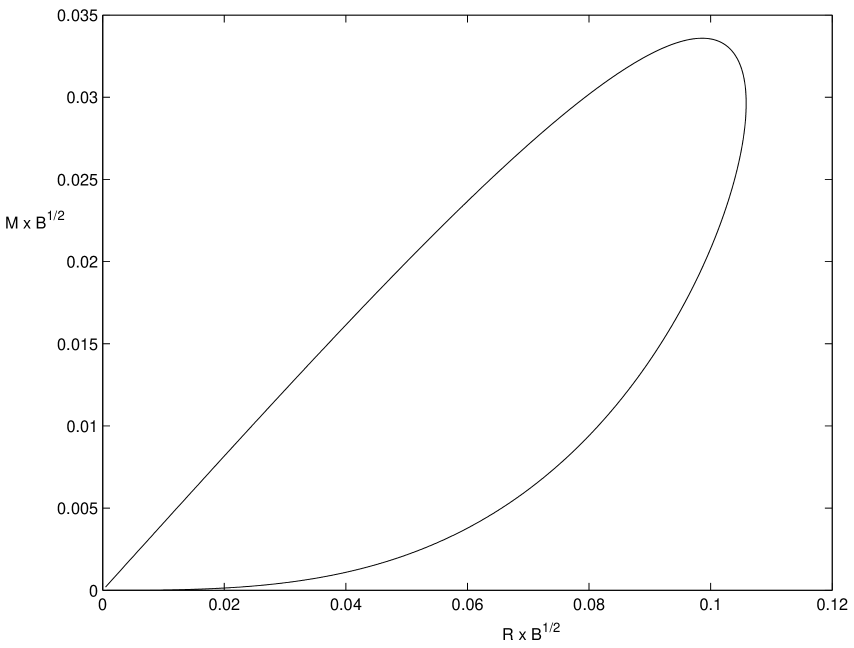
Figure 1: Mass-radius curve for the SUREOS constant energy density solution with $B$ at a fixed positive value. The curve is parametrized by the dimensionless parameter $k$ in the range $1/\sqrt{2}<k<\sqrt{2}$ or equivalently by the central pressure $p_{c}=\frac{2}{3}B(2k^{2}-1)/(2-k^{2})$ taking all positive values. The direction of increasing $k$ and $p_{c}$ is the counterclockwise one. The maximum of the curve is at $k\approx 1.133$ and separates this one-parameter family of solutions into a stable branch with $1/\sqrt{2}<k\lesssim 1.133$ and a branch with $1.133\lesssim k<\sqrt{2}$ having one unstable radial mode. A peculiar feature of this mass-radius curve is that it not only starts out from the origin $M=R=0$ at zero central pressure but also returns there in the limit of infinite central pressure.

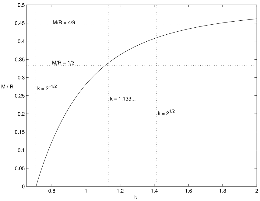
Figure 2: The compactness $M/R$ for the SUREOS constant energy solution, plotted as a function of the dimensionless parameter $k$. Although the discussion in this paper is restricted to non-negative values of $B$, which requires that $k\leq\sqrt{2}$, the plot has been continued into the negative $B$ sector $k>\sqrt{2}$ to display that the compactness then exceeds the perfect fluid Buchdahl limit value $M/R=4/9$ for sufficiently large $k$. In fact, as $k$ is taken to infinity the curve asymptotically approaches the horizon value $M/R=1/2$. Such extreme models having a surface arbitrarily close to the horizon have previously been investigated for other matter types, for charged perfect fluids by de Felice et al.[14, 15]. In the positive $B$ sector $1/\sqrt{2}<k<\sqrt{2}$ the solutions are stable up to $k\approx 1.133$, implying that the limiting compactness for the stable branch is $M/R\approx 0.3408$. Notably this value is slightly larger than $1/3$ and hence there are stable solutions that are ultracompact in the sense that their surfaces are inside $R=3M$ at which the exterior Schwarzschild solution has closed lightlike geodesics. At $k=\sqrt{2}$ (infinite central pressure when $B\neq 0$) the compactness is $M/R\approx 0.4096$.

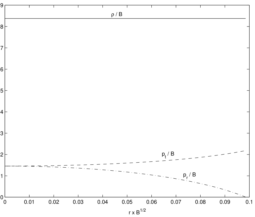
Figure 3: Energy density and pressure profiles for the marginally stable model with $k\approx 1.133$. The radius of this model is $R\approx 0.09857\times B^{-1/2}$. The radial (tangential) pressure is monotonically decreasing (increasing) for other values of $k$ as well.

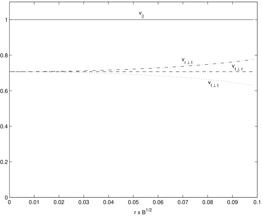
Figure 4: Profiles of the speeds of elastic wave propagation for the marginally stable model with $k\approx 1.133$. While the single longitudinal wave speed $v_{||}$ is always unity (speed of light) the principal transversal wave speeds $v_{r\perp t}$, $v_{t\perp r}$ and $v_{t\perp t}$ start out from the unsheared value $\sqrt{2}$ at the centre and diverges outwards as the pressure anisotropy increases. For smaller (larger) values of $k$, and thus of the central pressure, the profiles are qualitatively similar but the divergence is weaker (stronger). The transversal speed $v_{t\perp r}$ is however always exactly equal to $\sqrt{2}$.

4.1 Stability against radial perturbations

According to the results of paper II, the radial perturbations for the constant energy density solutions are governed by the first order system

$$\frac{d\zeta}{dx} =r_{0}\cos x\,[Y\zeta+P^{-1}\eta]$$ (59)

$$\frac{d\eta}{dx} =-r_{0}\cos x\,[(Q+\omega^{2}W)\zeta+Y\eta],$$ (60)

where the indendent variables $\zeta$ and $\eta$ are closely related to the lagrangian perturbations of the Schwarzschild radius and the radial pressure, respectively. Moreover $r_{0}=\sqrt{(2-k^{2})/(2\kappa B)}$ and

$$P =\frac{2\alpha^{3}}{\kappa r_{0}^{\;4}}\frac{(-\cos{2x}\sinh{kx}+{\textstyle\frac{1}{2}}k\sin{2x}\cosh{kx})\sinh^{2}{\!kx}}{\sin^{7}{\!x}\cos{x}}$$ (61)

$$Y =-\frac{1}{r_{0}}\frac{[(2+k^{2})\sin^{2}{\!x}+1]\sinh{kx}-{\textstyle\frac{1}{2}}k\sin{2x}\cosh{kx}}{(\cos{2x}\sinh{kx}-{\textstyle\frac{1}{2}}k\sin{2x}\cosh{kx})\sin{x}}$$ (62)

$$W =P\alpha^{-2}\frac{\tan^{2}\!x}{\sinh^{2}{\!kx}}$$ (63)

$$Q =Q_{1}+Q_{2}$$ (64)

$$Q_{1} =P\frac{4}{r_{0}^{\;2}}\frac{k^{2}\sin^{2}{\!x}\cosh^{2}{\!kx}-\cos{2x}\sinh^{2}{\!kx}}{\sin^{2}{\!2x}\sinh^{2}{\!kx}}$$ (65)

$$Q_{2} =P(Z+Y^{2})$$ (66)

$$Z =\frac{1}{r_{0}^{\;2}}\frac{3\cos{x}\left[(2\cos^{2}{\!x}+5)\sinh^{2}{\!kx}+k^{2}\sin^{2}{\!x}\,(5\cosh^{2}{kx}-3)\right]-k\sin{x}\,(1+{\textstyle\frac{25}{2}}\cos^{2}{\!x}+k^{2}\sin^{2}{\!x})\sinh{2kx}}{(\cos{2x}\sinh{kx}-{\textstyle\frac{1}{2}}k\sin{2x}\cosh{kx})\sin^{2}{\!x}\cos{x}\sinh{kx}}.$$ (67)

A regular solution to the system (59) and (60) should leave the centre according to

$$\zeta =Cr_{0}^{\;3}x^{3}+O(x^{5})$$ (68)

$$\eta =CP_{0}(3-Y_{0})+O(x^{2}),$$ (69)

where $C$ is an arbitrary constant and where $P_{0}$ and $Y_{0}$, as defined in paper II, are given by

$$P_{0} =\frac{2}{3}\frac{\alpha^{3}k^{3}(k^{2}+4)}{\kappa r_{0}^{\;2}}$$ (70)

$$Y_{0} =2.$$ (71)

At the surface of the star the lagrangian perturbation of the radial pressure should vanish, implying

$$\eta|_{x=x_{\mathrm{s}}}=0.$$ (72)

We have numerically determined the first two frequencies $\omega_{0}$ and $\omega_{1}$ of radial oscillations for $B>0$ and found that $\omega_{0}^{\;2}$ changes sign from positive to negative at $k\approx 1.133$, which to numerical precision coincides with the maximum mass model. As expected, $\omega_{1}^{\,2}$ is positive for all allowed values of $k$. The results are presented in figure 5.

Figure 5: The first two frequencies of radial oscillations for the family of constant energy density models with $B>0$. The squared frequencies as well as the stellar mass $M$ are plotted as functions of the dimensionless parameter $k$, displaying clearly that $\omega_{0}^{\;2}$ turns negative precisely at the maximum mass model having $k\approx 1.133$. Although partially cut out from the plot, the square of the first overtone frequency $\omega_{1}$ remains positive up to the infinite central pressure limit $k=\sqrt{2}$.

5 A solution with nonconstant energy density

The constant energy density of the family of solutions presented in the previous section comes about because the unsheared, i.e. compressional, energy density $\check{\rho}$ decreases outwards at exactly the same rate as the shearing energy density $\sigma=\rho-\check{\rho}$ inreases. Here we will briefly present a different SUREOS solution which is more realistic in the sense that the energy density as well as both principal pressures are monotonically outwards decreasing, just to illustrate that such solutions do exist. The solution was found for $B=0$ only and although we have made some attempts to generalise it to nonzero $B$ we have not been able to do so.

In Schwarzschild coordinates the spacetime metric for the solution has the simple analytic form

$$ds^{2}=\mathop{\rm sinc}\nolimits^{\!-2}{\!(r/r_{0})}\,(-\alpha^{2}dt^{2}+dr^{2})+r^{2}d\Omega^{2},\quad\mathop{\rm sinc}\nolimits{x}=\frac{\sin{x}}{x}.$$ (73)

To match the solution to a Schwarzschild exterior without rescaling the time coordinate, the constant $\alpha$ should be chosen as

$$\alpha=\mathop{\rm sinc}\nolimits^{2}{\!(R/r_{0})},$$ (74)

where $R$ is the radius of the star, i.e. $r=R$ is the surface of vanishing radial pressure, to be determined below. Regularity at the centre is clearly guaranteed by the fact that $\mathop{\rm sinc}\nolimits x=1$ at $x=0$. The energy density and principal pressures are given by

$$\kappa r^{2}\rho =1+\mathop{\rm sinc}\nolimits^{2}{\!(r/r_{0})}-2\mathop{\rm sinc}\nolimits{\!(r/r_{0})}\cos{\!(r/r_{0})}$$ (75)

$$\kappa r^{2}p_{r} =-1+3\mathop{\rm sinc}\nolimits^{2}{\!(r/r_{0})}-2\mathop{\rm sinc}\nolimits{\!(r/r_{0})}\cos{\!(r/r_{0})}$$ (76)

$$\kappa r^{2}p_{t} =\frac{2m}{r}=1-\mathop{\rm sinc}\nolimits^{2}{\!(r/r_{0})}$$ (77)

$$\rho_{c}=3p_{c}=\frac{1}{\kappa r_{0}^{\;2}}.$$ (79)

The profiles of these quantities are plotted in figure 6. The radial pressure drops to zero very close to $r=2r_{0}$, or more precisely

$$R\approx 1.9979\,r_{0},$$ (80)

implying $\alpha\approx 0.2075$ and $R/M\approx 2.5237$.

A similar analysis to that of section 4.1 reveals that the fundamental radial mode is unstable with squared frequency $\omega_{0}^{\;2}\approx-0.07017\,r_{0}^{-2}$ which for a typical neutron star with a radius of the order of 10 km corresponds to an e-folding time of about 0.4 ms. Clearly then, this solution is not very interesting on its own right, but if it could be generalised to a family with $B$ being a free parameter we expect there to be a stable branch of solutions.

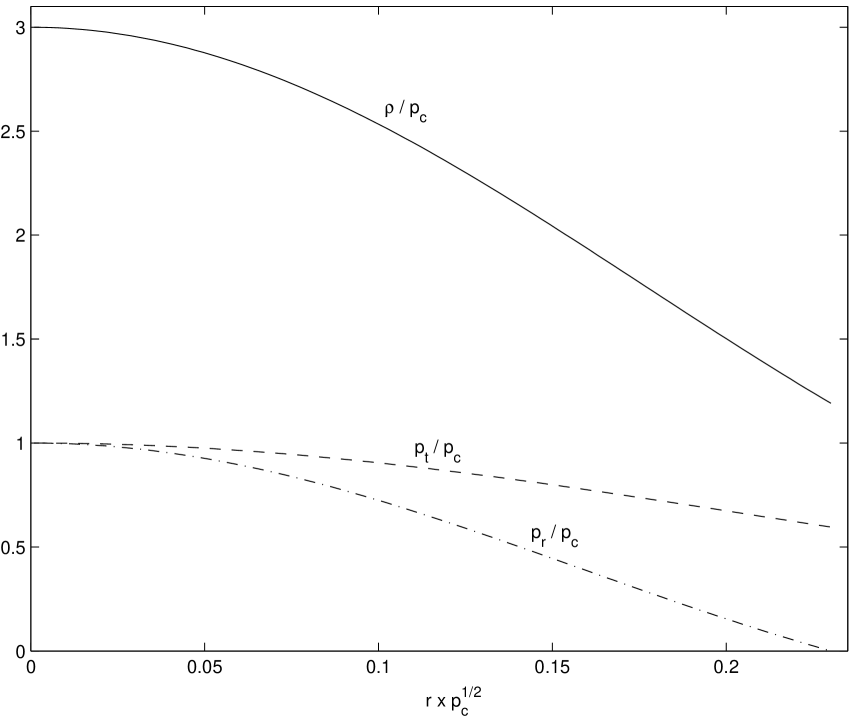
Figure 6: Energy density and pressure profiles for the $B=0$ solution with outwards decreasing energy density and eigenpressures.

6 Discussion and outlook

Exact solutions to the Einstein equations can very rarely be used to completely replace numerically obtained solutions, with a few important exceptions such as the Kerr-Newman family of black hole solutions. The reason is of course that it is almost always impossible to find an exact solution that obeys all restrictions that are imposed by requiring that the solution be astrophysically realistic. However, if an exact solution satisfies at least some basic criteria for physicality, that solution has the potential of being a useful tool for gaining qualitative insights. Furthermore it can be very useful as a test background model when doing numerical studies of various types of perturbations. The constant energy density family of exact SSS solutions with stiff ultrarigid equation of state does, in our opinion, satisfy the relevant list of basic criteria that renders it useful in these respects. In fact we have already used it in the present paper to test that our analysis and numerical codes for radial oscillations of spherically symmetric elastic matter models are behaving as expected; Clearly it cannot be a coincidence that we find the zeroth mode turning unstable for the maximum mass member of the family, to numerical precision. So far this had only been tested for the numerically integrated models presented in paper I, which all have moderate pressure anisotropies, but now we know that it also works as expected for models with more extreme anisotropies.

Since the presented method of generating SUREOS solutions does not rely upon spherical symmetry but only on stationarity and rigid motion, it would be very nice if one could also apply it to finding a rigidly rotating solution family. Although the equation of state is rather extreme, it is nevertheless always microstable and causal and hence, in our view, more physical than the equation of state $\rho+3p=\rho_{0}$ for Wahlquist’s rotating perfect fluid solution[16]. The latter equation of state fails to be microstable since the squared speed of sound $dp/d\rho$ is obviously negative.

Appendix

Since the principal longitudinal speed is equal to the speed of light, it is of interest to find out whether this speed can become superluminal when the propagation vector $\nu^{a}$ is perturbed around the principal unit vector $e_{\mu}^{\;a}$. For the SUREOS the Fresnel tensor can be written in the simple form

$$Q^{ab}=\rho h^{ab}+p^{ab}-L^{ab},$$ (81)

where $L^{ab}$ is the tensor

$$L^{ab}=\sum_{\sigma=1}^{3}(\rho-p_{\sigma}-2B)Z_{\sigma}^{\;a}Z_{\sigma}^{\;b}=2A\sum_{\sigma=1}^{3}n_{\sigma+1}^{\;2}n_{\sigma+2}^{\;2}Z_{\sigma}^{\;a}Z_{\sigma}^{\;b},\quad Z_{\sigma}^{\;a}=\epsilon^{abc}e_{\sigma b}\,\nu_{c}=\nu_{\sigma+1}\,e_{\sigma+2}^{\;a}-\nu_{\sigma+2}\,e_{\sigma+1}^{\;a}.$$ (82)

Thus the characteristic equation, which given a unit propagation vector $\nu^{a}=\sum_{\sigma=1}^{3}\nu_{\sigma}e_{\sigma}^{\;a}$ determines three propagation speeds $v$ and polarization vectors $\iota^{a}$, can in this case be rewritten in the convenient form

$$\left[(1-v^{2})(\rho h^{ab}+p^{ab})+L^{ab}\right]\iota_{b}=0.$$ (83)

Since all three vectors $Z_{\sigma}^{\;a}$ are orthogonal to $\nu^{a}$, so is the tensor $L^{ab}$ which means that the characteristic equation always has the solution

$$v^{2} =1$$ (84)

$$\iota_{a} =\nu_{a}$$ (85)

Since this result holds regardless of the choice of propagation vector $\nu^{a}$, we have proved the claim that the equation of state allows for a purely longitudinally polarized wave mode in all directions, i.e. not only principal directions which is the case generically. Moreover, the speed of these waves is direction independent and equal to the speed of light. Let us now consider $L^{ab}$ as a tensor on the two-space orthogonal to $\nu^{a}$ (and, of course, to $u^{a}$). As such, its determinant (or, rather, the determinant of the mixed tensor $L^{a}{}_{b}$) can be calculated according to

$${\textstyle\frac{1}{2}}L^{ab}L^{cd}\epsilon_{ac}\epsilon_{bd},\quad\epsilon_{ab}=\epsilon_{abc}\nu^{c}.$$ (86)

The result is

$${\textstyle\frac{1}{2}}L^{ab}L^{cd}\epsilon_{ac}\epsilon_{bd}=\sum_{\sigma=1}^{3}(\rho-p_{\sigma+1}-2B)(\rho-p_{\sigma+2}-2B)\nu_{\sigma}^{\;2}=4A^{2}n^{2}\sum_{\sigma=1}^{3}n_{\sigma}^{\;2}\nu_{\sigma}^{\;2}.$$ (87)

Clearly, this scalar can only be zero if at least one linear particle density vanishes which only happens if the material space mapping is degenerate which is disallowed. Now, with $L^{ab}$ being orthogonal to $\nu^{a}$ and of rank two, it follows that the only solution to the characteristic equation (83) with $v^{2}=1$ is the longitudinally polarized solution. For, if $\iota_{a}$ was to have a nonvanishing projection orthogonal to $\nu^{a}$, that projection would have to be annihilated by $L^{ab}$ which is impossible by the nondegeneracy property of the latter. As a corollary we thus have proved that the remaining two polarization modes always have propagation speeds less than unity. This follows from the facts that they should vary continuously with the propagation direction and that they are strictly less than unity for propagation in principal directions, in which case the polarization is purely transversal.

References

- [1] M. Delgaty and K. Lake, Comput. Phys. Commun. 115, 395 (1998).
- [2] R. L. Bowers and E. P. T. Liang, Astrophys. J. 188, 657 (1974).
- [3] M. Karlovini and L. Samuelsson, Class. Quantum Grav. 20, 3613 (2003).
- [4] M. Karlovini, L. Samuelsson, and M. Zarroug, Class. Quantum Grav. 21, 1559 (2004).
- [5] J. Kijowski and G. Magli, Gen. Rel. Grav. 24, 139 (1992).
- [6] E. Farhi and R. L. Jaffe, Phys. Rev. D 30, 2379 (1984).
- [7] Ya. B. Zel’dovich, Sov. Phys. JETP 14, 1143 (1962).
- [8] P. Haensel, in Relativistic Gravitation & Gravitational Radiation, edited by J. A. Marck and J. P. Lasota (Cambridge University Press, Cambridge, 1997).
- [9] B. Carter and H. Quintana, Proc. Roy. Soc. Lond. A 331, 57 (1972).
- [10] J. Hietarinta, Phys. Rep. 147, 87 (1987).
- [11] B. Carter, Phys. Rev. D 7, 1590 (1973).
- [12] H. Stephani et al., Exact Solutions of Einstein’s Field Equations, 2nd ed. (Cambridge University Press, Cambridge, UK, 2003).
- [13] W. H. Press et al., Numerical Recipes in C : The Art of Scientific Computing, 2nd ed. (Cambridge University Press, Cambridge, UK, 1992).
- [14] F. de Felice, Y. Yunqiang, and J. Fang, Mon. Not. R. Ast. Soc. 277, L17 (1995).
- [15] F. de Felice, L. Siming, and Y. Yunqiang, Class. Quantum Grav. 16, 2669 (1999).
- [16] H. D. Wahlquist, Phys. Rev. 172, 1291 (1968).