Radiation tails and boundary conditions for black hole evolutions

Abstract

Abstract

In numerical computations of Einstein’s equations for black hole spacetimes, it will be necessary to use approximate boundary conditions at a finite distance from the holes. We point out here that “tails,” the inverse power-law decrease of late-time fields, cannot be expected for such computations. We present computational demonstrations and discussions of features of late-time behavior in an evolution with a boundary condition.

I Introduction

There is at present great interest in the computation of the gravitational waves from the inspiral and merger of a pair of mutually orbiting black holesnumrel1 ; numrel2 ; numrel3 . To do such computations a solution of the initial value equations of general relativity is chosen on some initial spatial hypersurface, and the remaining Einstein equations are used to find the spacetime to the future of that initial surface. In principle, one can compute the evolved spacetime only in the domain of dependence of that initial surface, which means that the initial surface must be large, many times the radius of the initial binary orbit, if the spacetime is to be evolved for several orbital times. The computational demands for such a procedure make it unfeasible for the foreseeable future, although pseudospectral codes can help considerably in extending the size of the initial hypersurfacescheeletal . The alternative to a large initial hypersurface is a timelike boundary on the computation, typically at some large radius, at which appropriate approximate boundary conditions are specified. These boundary conditions are chosen to represent (approximately) the condition that no information moves inward through the boundary. One of the problems that workers in this field have recently turned to is that of appropriate boundary conditions, especially in connection with the preservation of gauge constraintsLSU ; frittelli ; winicour .

One of the features found in evolutions of perturbations in black holes spacetimes is the final latest-time behavior of the perturbation fields, a fall off in time $t$ as $1/t^{n}$ at a constant distance from the holeprice ; barack . This was first demonstrated for Schwarzschild holes in which case $n=2\ell+3$ for a multipole of index $\ell$ with compact initial support. For Kerr holes such tails also represent the latest time behavior, though there remains some controversy about the value of $n$krivan ; poisson ; burko_khanna . Most work on these tails has been done within linearized perturbation theory, though some computations with self-gravitating spherically symmetric scalar fields have also been carried outburko_ori ; gundlachetal ; scheeletal2 .

The purpose of the present paper is to point out that numerical computations with approximate boundary conditions cannot be expected to produce the correct late-time tails. A rough intuitive reason for this is that the late-time tails are produced by the scattering of radiation due to the curvature of spacetime. This scattering takes place far from the hole, and depends on the asymptotic large-distance nature of spacetime curvature. A boundary condition on a timelike surface at finite radius means that the asymptotic nature of the distant spacetime does not enter into the computation, so that the correct late-time tails cannot develop.

These ideas can be checked accurately in the Schwarzschild background. In this case linearized perturbations (scalar, electromagnetic, or gravitational) can be analyzed into multipoles $\psi=\sum\psi_{\ell m}(t,r)Y_{\ell m}(\theta,\phi)$, where $t,r,\theta,\phi$ are the standard Schwarzschild coordinates. The evolution of each multipole is described by a simple wave equationprice

$$\partial_{t}^{2}\psi(t,r)-\partial_{r*}^{2}\psi(t,r)+V(r)\psi(t,r)=0\;.$$ (1)

Here $c=G=1$ and, for simplicity, we have dropped the multipole indices on $\psi_{\ell m}(t,r)$ and on $V_{\ell}(r)$. The Regge-WheelerRW “tortoise coordinate” $r^{*}$ is defined by $r^{*}=r+2M\ln(r/2M-1)$, where $M$ is the mass of the Schwarzschild hole. In the limit $M\rightarrow 0$, that is, in flat spacetime, $r=r^{*}$ and the potential takes the form

$$V^{\rm flat}=\ell(\ell+1)/r^{*2}\ .$$ (2)

For this potential, the solution to Eq. (1) has a simple familiar form in terms of spherical Bessel functions, and has no tails.

If $M\neq 0$ there are important differences. For a scalar perturbation, the potential,

$$V^{\rm sc}(r)=\left(1-\frac{2M}{r}\right)\,\left[\frac{\ell(\ell+1)}{r^{2}}+\frac{2M}{r^{3}}\right]\,,$$ (3)

is typical of that for all perturbation fields. For $r^{*}\gg M$ this potential has the form

$$V^{\rm sc}=\frac{\ell(\ell+1)}{r^{*2}}\left[1+4M\;\frac{\ln(r^{*}/2M)}{r^{*}}+{\cal O}(M/r^{*})\right]\,.$$ (4)

It is the extra $\ln r^{*}/r^{*}$ term that is in Eq. (4), but missing in Eq. (2), that produces the $1/t^{2\ell+3}$ tailschingetal . To check this we define a toy potential

$$V^{\rm toy}=\frac{\ell(\ell+1)}{r^{*2}}\left[1+2MA\;\frac{\ln(r^{*}/2M)}{r^{*}}\right]\,,$$ (5)

with an adjustable parameter, $A$, that allows us to control the size of the extra term. Using this potential we have numerically evolved Eq. (1) with $\ell=1$why1 . The initial data, at time $t=0$, for this evolution was a time-symmetric Gaussian pulse $\psi=\exp(-0.1(r^{*}/2M+4)^{2})$. The results, for $\psi$ at $r^{*}=400M$, are shown as a function of time $t$ in Fig. 1.

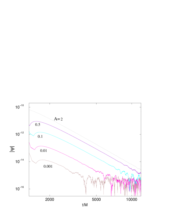
Figure 1: Late-time evolved solutions for different values of $A$, the coefficient of the scattering term in the toy potential described in the text. The absolute value of the scalar field $\psi$ is shown as a function of time $t$ at $r^{*}=400M$. Curves are labeled with the value of $A$.

The figure shows the straight lines in the log-log plot that indicate a power-law fall off in time. For all values of $A$ the slope is -5, consistent with the $2\ell+3$ rule. (At very late times each of the power-law tails disappears into round-off noise.) The results clearly show the sensitivity of the tail to the size of $A$. For $A=0$, of course, the toy potential becomes the flat spacetime potential centrifugal, and there is no tail. (The magnitude of the tail increases as $A$ is made larger, but this increase slows, and the magnitude of the tail appears to reach a limit.)

The argument against tails with finite boundary conditions, then, is that they depend on the asymptotic form of the potential. For the obvious Sommerfeld outgoing boundary condition

$$\psi_{,t}+\psi_{,r^{*}}=0\,,\mbox{ at $r^{*}=r^{*}_{\rm bc}$\,,}$$ (6)

the interior solution cannot “know” what the potential is for $r^{*}>r^{*}_{\rm bc}$, and hence the solution cannot develop a tail except at spacetime points whose domain of dependence lies within the outer boundary.

This argument, of course, is only suggestive. One can rebut it with the claim that a boundary condition could be made sufficiently precise so that it encodes the asymptotic form of the potential. A trivial example is the case $V=0$ and $r=r^{*}$, for which the general solution, in terms of an arbitrary outgoing function $f$, and an arbitrary ingoing function $g$, is

$$\psi=f(t-r)+g(t+r)\,.$$ (7)

In this case the outgoing boundary condition $\psi_{,t}-\psi_{,r}=0$ is exact; it constrains $g$ to be zero, the same condition as if the boundary were infinitely far away. A less trivial, but less useful case is the $M=0$, $\ell=1$ scalar equation . The general solution in this case is

$$\psi={f^{\prime}(t-r)}+\frac{f(t-r)}{r}\;+\;{g^{\prime}(t+r)}-\frac{g(t+r)}{r}\,,$$ (8)

where $f$ describes the outgoing part and $g$ the ingoing part. An exact boundary condition is

$$\left(\partial_{r}+\partial_{t}\right)^{2}\left[r^{2}\left(\partial_{r}+\partial_{t}\right)\psi\right]=0\,,$$ (9)

which constrains $g$ (more precisely $g^{{}^{\prime\prime\prime}}$) to vanish.

The cases in Eqs. (7) and (8) are special. In these cases the radiative part of the solution (the parts without $1/r$ factors) and the nonradiative parts are simply related. The nonradiative part is missing for Eq. (7), and for Eq. (8) the nonradiative part is a simple time intergral over the radiative part. This simplicity is related to Huygens’ principle. Note in particular that in Eq. (7) or (8) if $g=0$ and if $f$ has compact support, then the solution will be nonzero only for a finite time, and hence cannot have a power-law tail as a generic feature. The nonsimple non-Huygens solution for problems in which tails are generic will not, therefore, have an exact boundary condition that can be expressed as a finite number of differentiations as in Eq. (9).

II Evolutions with approximate boundary conditions

We now directly investigate the late-time behavior of solutions with approximate outgoing boundary condition of Eq. (6). The monopole $\ell=0$ case is studied so that the predicted slowly-falling $1/t^{3}$ tails stay well above the roundoff noise. The starting field is a purely outgoing pulse defined on the ingoing null ray $t+r^{*}=0$. On this ray, in terms of retarded time $u\equiv t-r^{*}$, the form of $\psi$ is specified to be $\psi=\left[u(u-8M)/16M^{2}\right]^{8}$, for $0<u<8M$, and $\psi=0$ for $u<0$ or $u>8M$. The initial data at $t=0$ then is approximately an outgoing pulse (satisfying $\psi_{,r^{*}}=-\psi_{,t}$) confined between $r^{*}=-8M$ and $r^{*}=0$, centered at $r^{*}=-4M$ with a peak value $\psi=1$ there. The left boundary for all $\ell=0$ computations is at $r^{*}=-500M$, where the sommerfeld condition $\psi_{,r^{*}}=\psi_{,t}$ is imposed. The right boundary is placed at different locations $r^{*}_{\rm bc}$, and the condition $\psi_{,r^{*}}=-\psi_{,t}$ is imposed.

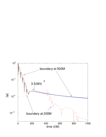
Figure 2: The scalar monopole $\psi$ evolving from an initially outgoing pulse near $r^{*}=0$. The field $\psi$ is plotted as a function of time at $r^{*}=0$ for two different values of $r_{\rm bc}^{*}$, at $500M$ and $200M$. The two curves are identical up to time $t=400M$. A curve proportional to $1/t^{3}$ is included for comparison.

Figure 2 shows the time profile of $\psi$ developing from the initial pulse. The value of $\psi$ at the fixed position $r^{*}=0$ is shown as a function of time for outgoing boundary locations $r^{*}_{\rm bc}=500M$ (solid curve) and at $r^{*}_{\rm bc}=200M$ (dot-dashed curve). Since the results are shown only up to $t=1000M$, the field at $r^{*}=0$, shown by the solid curve, has not yet been influenced by the interaction of the boundaries at $\pm 500M$ with the evolution of the initial pulse from $r^{*}=0$. The solid curve then shows the “boundaryless” behavior of the field evolving completely within the domain of dependence of the initial data. That field goes through quasinormal ringing up to around $t=150M$, then around $t=300M$ becomes a power-law tail. Since the plot is a semilog plot, not a log-log plot, the tail is not a straight line, and a ${\rm constant}/t^{3}$ curve is provided to illustrate the tail nature of the solid curve. The dot-dashed curve for the $r^{*}_{\rm bc}=200M$ outer boundary is identical to the solid curve up to $t=400M$. In particular, from $t\approx 300M$ to $t=400M$ the field starts to take the form of a power-law tail, but at $t=400M$ waves reflected from the $r^{*}_{\rm bc}=200M$ boundary arrive at $r^{*}=0$ and a new oscillatory behavior ensues due to the influence of the boundary.

A complementary viewpoint on the boundary influence is given in Fig. 3, in which spatial profiles of evolved fields are shown at the moment of time $t=500M$. As in Fig. 2, the solid curve corresponds to an outer boundary at $r^{*}=500M$, and the dot-dashed curve to an outer boundary at $r^{*}=200M$. The solid curve indicates that at $t=500M$ the unit-height pulse has reached the outer boundary. In the absence of scattering this would be the only feature of the plot, but due to scattering there are quasinormal bumps created between $r^{*}\approx 370M$ and $500M$. Waves scattered inward also create quasinormal bumps between $r^{*}\approx-300M$ and $-500M$. From $r^{*}\approx-300M$ to $\approx 370M$ the solid curve shows the spatial profile of the tail behavior. The dot-dashed curve shows that reflections of the inital pulse off the $r^{*}=200M$ boundary have reached $r^{*}=-100M$ and have “contaminated” the spatial profile from $r^{*}=-100M$ to $200M$. The spatial profile from $r^{*}=-100M$ to $200M$ shows spatial oscillations similar to the temporal oscillations that appear in Fig. 2.

III Boundary-induced quasinormal ringing

Figure 3: Spatial profile of the scalar monopole $\psi$ evolving from an initially outgoing pulse. Here $\psi$ is plotted at $t=500M$ for values of $r_{\rm bc}^{*}$ at $500M$ and $200M$. The curves are identical for $r^{*}\leq-100M$ where the field has not yet been influenced by reflections of the initial pulse off the $200M$ boundary.

The nature of the boundary-induced oscillations is made clearer in Fig. 4, which shows the time profiles for outer boundaries at $100M$, $50M$, $25M$. (For larger values of $r^{*}_{\rm bc}$ similar oscillations develop at later times.) The late-time results for the $50M$ and $25M$ profiles indicates a constant-period oscillation, and the straight-line envelope of the oscillations in the semilog plot indicates an exponential damping. The natural interpretation is that these damped oscillations are a new form of quasinormal ringing. The “old” form is the familiar quasinormal ringing of a black holevishnature ; livingrev ; nollert , like that in Fig. 2 for $t/M$ less than $\sim 150$. This is a real physical phenomenon associated with the black hole spactime. In Fig. 4 we see oscillations that are not physical in this sense, but are numerical artifacts, the strongly damped oscillations of a leaky cavity created by the outer boundary and the curvature potential $V$ near its peak at $r^{*}=0$. Some evidence for this is the dependence of the period of the oscillations on $r^{*}_{\rm bc}$. The longer cavity of the $50M$-boundary case creates longer oscillation periods than the cavity of the $25M$-boundary. The less-clearly defined oscillations of the $100M$ have yet longer periods.

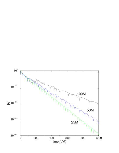
Figure 4: Evolution of the $\psi$ monopole for Sommerfeld outgoing conditions on close boundaries. The time profiles are for an initial outgoing pulse near $r^{*}=0$. Results are shown for outer boundaries at locations $r*=100M$, $50M$, and $25M$.

The leaky-cavity interpretation is supported by the plot in Fig. 5 showing the period $T$ for a full oscillation (the width of a pair of “bumps” in Fig. 4) of the late time features, as a function of $r^{*}_{\rm bc}$, the location of the outer boundary. The uncertainty in the period is around 2%, both due to truncation error in the evolution of $\psi$, and due to the extraction of $T$ from the late time results. For $r^{*}_{\rm bc}$ larger than $\sim 100M$ the period quite accurately follows the linear relation $T/M=-30+2.9(r^{*}_{\rm bc}/M)$, confirming the view that these late time oscillations are resonances of a cavity created by the outer boundary. For $r^{*}_{\rm bc}$ less than $\sim 100M$ it is not surprising that the details near the peak of the curvature potential $V$ would complicate the relationship; for large values of $r^{*}_{\rm bc}$ the details of the curvature potential become unimportant. What is

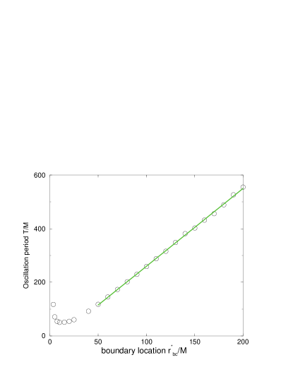
Figure 5: The period $T$ for a full oscillation (two “bumps”) as a function of the location $r^{*}_{\rm bc}$ of the outer boundary. The straight line $T/M=-30+2.9(r^{*}_{\rm bc}/M)$ is the least-squares fit to the results for $r^{*}_{\rm bc}=100M$ and larger.

at first surprising in the linear relationship is the coefficient $2.9$. This means that the number of half-wavelengths inside the “cavity” is not an integer; one would naively expect the period $T$ to be equal to the cavity length, or an integer multiple of half the cavity length. But our naive expectations are based on the simple boundary condition that the field or its normal derivative vanish. In our artificial cavity the outgoing boundary conditions does neither. For a constant-frequency oscillation the outgoing boundary condition, in effect, imposes a relationship between the field and its normal derivative. Computations with simple toy models have confirmed that with such boundary conditions a resonance of the cavity will not contain an integer number of half wavelengths.

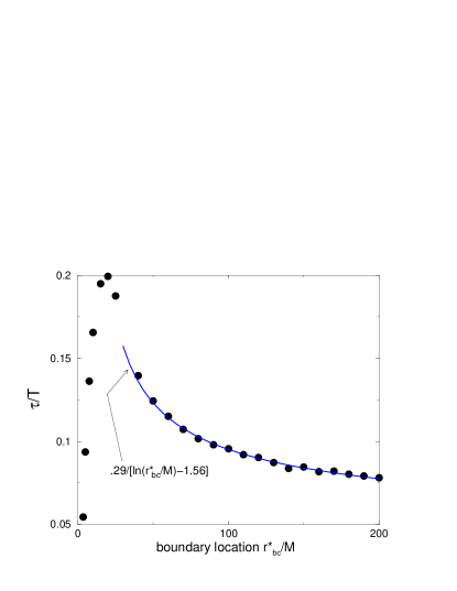
Figure 6: The time constant $\tau$ for the envelope of the decaying oscillations, divided by $T$, the period of the oscillations, as a function of the location $r^{*}_{\rm bc}$ of the outer boundary. The thick solid curve shows a heuristic model for $\tau$.

The leaky-cavity viewpoint on the outer boundary suggests a way to quantify the effectiveness of the outer boundary condition. The more effective the outer boundary condition is, the more quickly the cavity modes should die out. If we characterize the effective reflectivity of the outer boundary as $R$, and let $N$ represent the number of reflections from the outer boundary, then the amplitude should fall off as $R^{N}$. We can take $N$ to be the time $t$ divided by some measure of the time for a reflection. For generality we will take this to be $\kappa_{1}T$, were $\kappa_{1}$ is some constant, and $T$ is the period for an oscillation. The cavity oscillations should then die off as $R^{t/(\kappa_{1}T)}$, or as $\exp(-t/\tau)$, where the damping time $\tau$ is $-T\kappa_{1}/\ln(R)$. The outgoing boundary condition is expected to improve as $r^{*}_{\rm bc}$ increasesreflectivity , so it is interesting to make the ansatz $R=\kappa_{2}M/r^{*}_{\rm bc}$. This model predicts $\tau/T=\kappa_{1}/\left[\log(r^{*}_{\rm bc}/M)-\log(\kappa_{2})\right]$. Figure 6 shows $\tau/T$ for a range of outer boundary locations $r^{*}_{\rm bc}$; the uncertainty here, as in Fig. 5, is no worse than 2% at any $r^{*}_{\rm bc}$. The large-$r^{*}_{\rm bc}$ results in Fig. 6 do show a gradual decrease of $\tau/T$ with increasing $r^{*}_{\rm bc}$, as expected. Our heuristic model for $\tau$ is fit to those results by eye, and is plotted in Fig. 6. That fit corresponds to reflectivity $~{}4.8M/r^{*}_{\rm bc}$, or $\sim 5$% for a boundary at $100M$. The plot of the heuristic model gives an appearance of reasonable agreement except for small values of $r^{*}_{\rm bc}$, but with two adjustable parameters in the fit, this agreement can only be said to be weakly suggestive.

IV Summary and discussion

We have shown that finite-radius boundary conditions prevent the formation of power-law tails of perturbations in black hole spacetimes. In place of a tail, the latest-time feature of a computation will be a new form of quasinormal oscillation. Unlike black hole oscillations, these oscillations are not physical phenomena; they are numerical artifacts introduced by the imperfect outgoing condition at the outer boundary.

In numerical relativity, these oscillation will probably not be a serious practical difficulty. The goal of present numerical relativity work is a better understanding of strong field nonlinear dynamics. Numerical codes in the forseeable future will not be able to run long enough for the boundary-induced oscillations to appear, nor are they likely to be accurate enough to deal with such a weak field phenomenon.

These limitations of running time and accuracy do not apply when the Lazaruslazarus method is used in a problem involving the formation of a final black hole. That method uses the solution computed by a fully nonlinear numerical evolution code as initial data for further evolution by black hole perturbation theory. The nonlinear numerical evolution would, of necessity, use timelike boundaries, but the numerical cavity oscillations would not develop in the limited time for which the evolutions run. In principle, the subsequent Lazarus evolution could be used without boundary conditions, i.e., with evolution only within the domain of dependence of the initial data inherited from the fully nonlinear numerical code. Such boundaryless Lazarus evolutions would exhibit power-law tails, but the tails would be strongly affected by boundary effects contained in the initial data inherited from the nonlinear evolution. In practice, Lazarus evolutions are not boundaryless. Rather, to reduce memory requirements, timelike boundary conditions are used in the Lazarus perturbation evolutions. These evolutions should contain boundary-induced artifacts of the type we have discussed above. But these artifacts would be miniscule, and of no concern for most applications of black hole evolution, with or without Lazarus.

V Acknowledgment

We gratefully acknowledge the support of the National Science Foundation to the University of Utah, under grants PHY9734871 and PHY0244605. We thank Gioel Calabrese, Manuel Tiglio, Luis Lehner and Jorge Pullin for discussions and suggestions about boundary effects. We thank Carlos Lousto for discussions of the boundary treatment in the Lazarus method.

References

- (1) S. Brandt et al., Phys. Rev. Lett. 85, 5496 (2000).
- (2) M. Alcubierre et al., Phys. Rev. Lett. 87, 271103 (2001).
- (3) L. Lehner, Class. Quantum Grav. 18, R25 (2001).
- (4) M. Scheel et al., Phys. Rev. D 66, 124005 (2002).
- (5) G. Calabrese, L. Lehner, and M. Tiglio, Phys. Rev. D 65, 104031 (2002).
- (6) S. Frittelli and R. Gomez, Class. Quantum Grav. 20, 2379 (2003).
- (7) B. Szilagyi and J. Winicour, Phys. Rev. D68, 041501 (2003).
- (8) R. H. Price, Phys. Rev. D5, 2419 (1972).
- (9) L. Barack, Phys. Rev. D59, 044016 (1999); Phys. Rev. D59, 044017 (1999).
- (10) W. Krivan, Phys. Rev. D 60, 101501 (1999).
- (11) E. Poisson, Phys. Rev. D 66, 044008 (2002).
- (12) L. M. Burko and G. Khanna, Phys. Rev. D67 081502, (2003).
- (13) C. Gundlach, R. H. Price and J. Pullin, Phys. Rev. D49, 890 (1994).
- (14) L. M. Burko and A. Ori, Phys. Rev. D56, 7820 (1997).
- (15) M. A. Scheel et al. preprint gr-qc/0305027.
- (16) T. Regge and J. A. Wheeler, Phys. Rev. 108, 1063 (1957).
- (17) E. S. C. Ching et al., Phys. Rev. Lett. 74, 2414 (1995).
- (18) Our subsequent computations will use , but here we use to make it clear that there can be a nonzero potential (the , case) without tails.
- (19) C.V. Vishveshwara, Nature, 227, 936 (1970).
- (20) K. D. Kokkotas and B. G. Schmidt, Living Rev. Relativ. 2, 2 (1999).
- (21) H.-P. Nollert, Class. Quantum Grav. 16, R159 (1999).
- (22) The usual argument is that the error in the outgoing boundary condition is of order . The wavelength of our “cavity oscillations” is proportional to . It would be consistent, therefore, to suggest that should be independent of , and our numerical results are more-or-less compatible with this.
- (23) J. Baker, M. Campanelli, and C. Lousto, Phys. Rev. D.65, 044001 (2002).