Thin shells around traversable wormholes

Abstract

Applying the Darmois-Israel thin shell formalism, we construct static and dynamic thin shells around traversable wormholes. Firstly, by applying the cut-and-paste technique we apply a linearized stability analysis to thin-shell wormholes in the presence of a generic cosmological constant. We find that for large positive values of the cosmological constant, i.e., the Schwarzschild-de Sitter solution, the regions of stability significantly increase relatively to the Schwarzschild case, analyzed by Poisson and Visser. Secondly, we construct static thin shell solutions by matching an interior wormhole solution to a vacuum exterior solution at a junction surface. In the spirit of minimizing the usage of exotic matter we analyze the domains in which the weak and null energy conditions are satisfied at the junction surface. The characteristics and several physical properties of the surface stresses are explored, namely, we determine regions where the sign of tangential surface pressure is positive and negative (surface tension). An equation governing the behavior of the radial pressure across the junction surface is deduced. Specific dimensions of the wormhole, namely, the throat radius and the junction interface radius, are found by taking into account the traversability conditions, and estimates for the traversal time and velocity are also determined.

I Introduction

Interest in traversable wormholes, as hypothetical shortcuts in spacetime, has been rekindled by the classical paper by Morris and Thorne Morris . The subject has also served to stimulate research in several branches, for instance, the violation of the energy conditions VisserBOOK ; VisserEC , closed timelike curves and the associated difficulties in causality violation VisserBOOK ; VissEC ; LoboCTC , and superluminal travel LoboSLT , amongst others.

As the violation of the energy conditions is a problematic issue, depending on one’s point of view, it is useful to minimize the usage of exotic matter. For instance, an elegant way of achieving this, is to construct a simple class of wormhole solutions using the cut and paste technique, implemented by Visser VisserBOOK ; Visser1 ; Visser2 , in which the exotic matter is concentrated at the wormhole throat. The surface stress-energy tensor components of the exotic matter at the throat are determined, invoking the Darmois-Israel formalism Darmois ; Israel ; Papahamoui . These thin-shell wormholes are extremely useful as one may apply a stability analysis for the dynamical cases, either by choosing specific surface equations of state eqstate1 ; eqstate2 ; eqstate3 , or by considering a linearized stability analysis around a static solution Poisson ; Lobolinear , in which a parametrization of the stability of equilibrium is defined, so that one does not have to specify a surface equation of state. In Lobolinear , the generalization of the Poisson-Visser linearized analysis Poisson for thin-shell wormholes was done in the presence of a non-vanishing cosmological constant. It was found that for large positive values of $\Lambda$, i.e., the Schwarzschild-de Sitter solution, the regions of stability significantly increase relatively to the Schwarzschild case analyzed by Poisson and Visser.

As an alternative to these thin-shell wormholes, one may also consider that the exotic matter is distributed from the throat to a radius $a$, where the solution is matched to an exterior vacuum spacetime. Several simple cases were analyzed in Morris , but one may invoke the Darmois-Israel formalism to consider a broader class of solutions. Thus, the thin shell confines the exotic matter threading the wormhole to a finite region, with a delta-function distribution of the stress-energy tensor on the junction surface. The motivation of this analysis resides in minimizing the usage of exotic matter threading the interior wormhole solution, which in principle may be made arbitrarily small VKD ; Viss , and imposing that the surface stresses of the thin shell obey the energy conditions. One may generalize and systematize Lobo the particular case of a matching with a constant redshift function and a null surface energy density on the junction boundary, studied in LLQ . A similar analysis for the plane symmetric case, with a negative cosmological constant, is done in LL . The plane symmetric traversable wormhole is a natural extension of the topological black hole solutions found by Lemos lemos1 ; lemos2 ; lemos3 ; zanchin , upon addition of exotic matter. These plane symmetric wormholes may be viewed as domain walls connecting different universes. They may have planar topology, and upon compactification of one or two coordinates, cylindrical topology or toroidal topology, respectively.

This paper is organized as follows. In Section II the Darmois-Israel thin shell formalism is briefly reviewed. In Section III, a linearized stability analysis is studied in the presence of a generic cosmological constant Lobolinear . In Section IV we match an interior wormhole spacetime to an exterior vacuum solution and find specific regions where the energy conditions at the junction are obeyed Lobo ; we also analyze the physical properties and characteristics of the surface stresses, namely, we find domains where the tangential surface pressure is positive or negative (surface tension); we deduce an expression governing the behavior of the radial pressure across the junction boundary; and finally, we determine specific dimensions of the wormhole by taking into account the traversability conditions and find estimates for the traversal time and velocity. Finally, in Section V, we conclude.

II Overview of the Darmois-Israel formalism

Consider two distinct spacetime manifolds, ${\cal M_{+}}$ and ${\cal M_{-}}$, with metrics given by $g_{\mu\nu}^{+}(x^{\mu}_{+})$ and $g_{\mu\nu}^{-}(x^{\mu}_{-})$, in terms of independently defined coordinate systems $x^{\mu}_{+}$ and $x^{\mu}_{-}$. The manifolds are bounded by hypersurfaces $\Sigma_{+}$ and $\Sigma_{-}$, respectively, with induced metrics $g_{ij}^{+}$ and $g_{ij}^{-}$. The hypersurfaces are isometric, i.e., $g_{ij}^{+}(\xi)=g_{ij}^{-}(\xi)=g_{ij}(\xi)$, in terms of the intrinsic coordinates, invariant under the isometry. A single manifold ${\cal M}$ is obtained by gluing together ${\cal M_{+}}$ and ${\cal M_{-}}$ at their boundaries, i.e., ${\cal M}={\cal M_{+}}\cup{\cal M_{-}}$, with the natural identification of the boundaries $\Sigma=\Sigma_{+}=\Sigma_{-}$.

The three holonomic basis vectors $e_{(i)}=\partial/\partial\xi^{i}$ tangent to $\Sigma$ have the following components $e^{\mu}_{(i)}|_{\pm}=\partial x_{\pm}^{\mu}/\partial\xi^{i}$, which provide the induced metric on the junction surface by the following scalar product

$$g_{ij}=e_{(i)}\cdot e_{(j)}=g_{\mu\nu}e^{\mu}_{(i)}e^{\nu}_{(j)}|_{\pm}.$$ (1)

We shall consider a timelike junction surface $\Sigma$, defined by the parametric equation of the form $f(x^{\mu}(\xi^{i}))=0$. The unit normal $4-$vector, $n^{\mu}$, to $\Sigma$ is defined as

$$n_{\mu}=\pm\,\left|g^{\alpha\beta}\,\frac{\partial f}{\partial x^{\alpha}}\,\frac{\partial f}{\partial x^{\beta}}\right|^{-1/2}\;\frac{\partial f}{\partial x^{\mu}}\,,$$ (2)

with $n_{\mu}\,n^{\mu}=+1$ and $n_{\mu}e^{\mu}_{(i)}=0$. The Israel formalism requires that the normals point from ${\cal M_{-}}$ to ${\cal M_{+}}$ Israel .

The extrinsic curvature, or the second fundamental form, is defined as $K_{ij}=n_{\mu;\nu}e^{\mu}_{(i)}e^{\nu}_{(j)}$, or

$$K_{ij}^{\pm}=-n_{\mu}\left(\frac{\partial^{2}x^{\mu}}{\partial\xi^{i}\,\partial\xi^{j}}+\Gamma^{\mu\pm}_{\;\;\alpha\beta}\;\frac{\partial x^{\alpha}}{\partial\xi^{i}}\,\frac{\partial x^{\beta}}{\partial\xi^{j}}\right)\,.$$ (3)

Note that for the case of a thin shell $K_{ij}$ is not continuous across $\Sigma$, so that for notational convenience, the discontinuity in the second fundamental form is defined as $\kappa_{ij}=K_{ij}^{+}-K_{ij}^{-}$.

Now, the Lanczos equations follow from the Einstein equations for the hypersurface, and are given by

$$S^{i}_{\;j}=-\frac{1}{8\pi}\,(\kappa^{i}_{\;j}-\delta^{i}_{\;j}\kappa^{k}_{\;k})\,,$$ (4)

where $S^{i}_{\;j}$ is the surface stress-energy tensor on $\Sigma$.

The first contracted Gauss-Kodazzi equation or the “Hamiltonian” constraint

$$G_{\mu\nu}n^{\mu}n^{\nu}=\frac{1}{2}\,(K^{2}-K_{ij}K^{ij}-\,^{3}R)\,,$$ (5)

with the Einstein equations provide the evolution identity

$$S^{ij}\overline{K}_{ij}=-\left[T_{\mu\nu}n^{\mu}n^{\nu}-\Lambda/8\pi\right]\,.$$ (6)

The convention $\left[X\right]\equiv X^{+}|_{\Sigma}-X^{-}|_{\Sigma}$ and $\overline{X}\equiv(X^{+}|_{\Sigma}+X^{-}|_{\Sigma})/2$ is used.

The second contracted Gauss-Kodazzi equation or the “ADM” constraint

$$G_{\mu\nu}e^{\mu}_{(i)}n^{\nu}=K^{j}_{i|j}-K,_{i}\,,$$ (7)

with the Lanczos equations gives the conservation identity

$$S^{i}_{j|i}=\left[T_{\mu\nu}e^{\mu}_{(j)}n^{\nu}\right]\,.$$ (8)

In particular, considering spherical symmetry considerable simplifications occur, namely $\kappa^{i}_{\;j}={\rm diag}\left(\kappa^{\tau}_{\;\tau},\kappa^{\theta}_{\;\theta},\kappa^{\theta}_{\;\theta}\right)$. The surface stress-energy tensor may be written in terms of the surface energy density, $\sigma$, and the surface pressure, $p$, as $S^{i}_{\;j}={\rm diag}(-\sigma,p,p)$. The Lanczos equations then reduce to

$$\sigma = -\frac{1}{4\pi}\,\kappa^{\theta}_{\;\theta}\,,$$ (9)

$$p = \frac{1}{8\pi}(\kappa^{\tau}_{\;\tau}+\kappa^{\theta}_{\;\theta})\,.$$ (10)

III Cut and paste technique: Thin-shell wormholes with a cosmological constant

In this section we shall construct a class of wormhole solutions, in the presence of a cosmological constant, using the cut-and-paste technique. Consider the unique spherically symmetric vacuum solution, i.e.,

$$ds^{2}=-\left(1-\frac{2M}{r}-\frac{\Lambda}{3}r^{2}\right)\,dt^{2}+\left(1-\frac{2M}{r}-\frac{\Lambda}{3}r^{2}\right)^{-1}\,dr^{2}+r^{2}\,(d\theta^{2}+\sin^{2}{\theta}\,d\phi^{2}).$$ (11)

If $\Lambda>0$, the solution is denoted by the Schwarzschild-de Sitter metric. For $\Lambda<0$, we have the Schwarzschild-anti de Sitter metric, and of course the specific case of $\Lambda=0$ is reduced to the Schwarzschild solution. Note that the metric $(1)$ is not asymptotically flat as $r\rightarrow\infty$. Rather, it is asymptotically de Sitter, if $\Lambda>0$, or asymptotically anti-de Sitter, if $\Lambda<0$. But, considering low values of $\Lambda$, the metric is almost flat in the range $M\ll r\ll 1/\sqrt{\Lambda}$. For values below this range, the effects of $M$ dominate, and for values above the range, the effects of $\Lambda$ dominate, as for large values of the radial coordinate the large-scale structure of the spacetime must be taken into account.

The specific case of $\Lambda=0$ is reduced to the Schwarzschild solution, with a black hole event horizon at $r_{b}=2M$. Consider the Schwarzschild-de Sitter spacetime, $\Lambda>0$. If $0<9\Lambda M^{2}<1$, the factor $g(r)=(1-2M/r-\Lambda r^{2}/3)$ possesses two positive real roots, $r_{b}$ and $r_{c}$, corresponding to the black hole and the cosmological event horizons of the de Sitter spacetime, respectively, given by

$$r_{b} = 2\Lambda^{-1/2}\,\cos(\alpha/3)\,,$$ (12)

$$r_{c} = 2\Lambda^{-1/2}\,\cos(\alpha/3+4\pi/3)\,,$$ (13)

where $\cos\alpha\equiv-3M\Lambda^{1/2}$, with $\pi<\alpha<3\pi/2$. In this domain we have $2M<r_{b}<3M$ and $r_{c}>3M$.

For the Schwarzschild-anti de Sitter metric, with $\Lambda<0$, the factor $g(r)=\left(1-2M/r+|\Lambda|r^{2}/3\right)$ has only one real positive root, $r_{b}$, given by

$$r_{b}=\left(\frac{3M}{|\Lambda|}\right)^{1/3}\left(\sqrt[3]{1+\sqrt{1+\frac{1}{9|\Lambda|M^{2}}}}+\sqrt[3]{1-\sqrt{1+\frac{1}{9|\Lambda|M^{2}}}}\;\right),$$ (14)

corresponding to a black hole event horizon, with $0<r_{b}<2M$.

III.1 The cut-and-paste construction

Given this, we may construct a wormhole solution, using the cut-and-paste technique VisserBOOK ; Visser1 ; Visser2 . Consider two vacuum solutions with $\Lambda$ and remove from each spacetime the region described by

$$\Omega_{\pm}\equiv\left\{r_{\pm}\leq a|\,a>r_{b}\right\}\,,$$ (15)

where $a$ is a constant and $r_{b}$ is the black hole event horizon, corresponding to the Schwarzschild-de Sitter and Schwarzschild-anti de Sitter solutions, equation (12) and equation (14), respectively. The removal of the regions results in two geodesically incomplete manifolds, with boundaries given by the following timelike hypersurfaces

$$\Sigma_{\pm}\equiv\left\{r_{\pm}=a|\,a>r_{b}\right\}\,.$$ (16)

Identifying these two timelike hypersurfaces, $\Sigma_{+}=\Sigma_{-}$, results in a geodesically complete manifold, with two regions connected by a wormhole and the respective throat situated at $\Sigma$. The wormhole connects two regions, asymptotically de Sitter or anti-de Sitter, for $\Lambda>0$ and $\Lambda<0$, respectively.

The intrinsic metric at $\Sigma$ is given by

$$ds^{2}_{\Sigma}=-d\tau^{2}+a^{2}(\tau)\,(d\theta^{2}+\sin^{2}{\theta}\,d\phi^{2})\,,$$ (17)

where $\tau$ is the proper time as measured by a comoving observer on the wormhole throat.

III.2 The surface stresses

The imposition of spherical symmetry is sufficient to conclude that there is no gravitational radiation, independently of the behavior of the wormhole throat. The position of the throat is given by $x^{\mu}(\tau,\theta,\phi)=(t(\tau),a(\tau),\theta,\phi)$, and the respective $4$-velocity is

$$U^{\mu}=\left(\frac{\sqrt{1-2M/a-\Lambda a^{2}/3+\dot{a}^{2}}}{1-2M/a-\Lambda a^{2}/3},\dot{a},0,0\right)\,,$$ (18)

where the overdot denotes a derivative with respect to $\tau$.

The unit normal to the throat may be determined by equation (2) or by the contractions, $U^{\mu}n_{\mu}=0$ and $n^{\mu}n_{\mu}=+1$, and is given by

$$n^{\mu}=\left(\frac{\dot{a}}{1-2M/a-\Lambda a^{2}/3},\sqrt{1-2M/a-\Lambda a^{2}/3+\dot{a}^{2}},0,0\right)\,.$$ (19)

Using equation (3), equation (11) and equation (19), the non-trivial components of the extrinsic curvature are given by

$$K^{\theta\;\pm}_{\;\,\theta} = \pm\frac{1}{a}\sqrt{1-2M/a-\Lambda a^{2}/3+\dot{a}^{2}}\;,$$ (20)

$$K^{\tau\;\pm}_{\;\,\tau} = \pm\frac{M/a^{2}-\Lambda a/3+\ddot{a}}{\sqrt{1-2M/a-\Lambda a^{2}/3+\dot{a}^{2}}}\;,$$ (21)

Thus, the Einstein field equations, equations (9)-(10), with equations (20)-(21), then provide us with the following surface stresses

$$\sigma = -\frac{1}{2\pi a}\sqrt{1-2M/a-\Lambda a^{2}/3+\dot{a}^{2}}\,,$$ (22)

$$p = \frac{1}{4\pi a}\;\frac{1-M/a-2\Lambda a^{2}/3+\dot{a}^{2}+a\ddot{a}}{\sqrt{1-2M/a-\Lambda a^{2}/3+\dot{a}^{2}}}\,.$$ (23)

We also verify that the above equations imply the conservation of the surface stress-energy tensor

$$\dot{\sigma}=-2\left(\sigma+p\right)\frac{\dot{a}}{a}$$ (24)

or

$$\frac{d\left(\sigma A\right)}{d\tau}+p\,\frac{dA}{d\tau}=0\,,$$ (25)

where $A=4\pi a^{2}$ is the area of the wormhole throat. The first term represents the variation of the internal energy of the throat, and the second term is the work done by the throat’s internal forces.

III.3 Linearized stability analysis

Equation (22) may be recast into the following dynamical form

$$\dot{a}^{2}-\frac{2M}{a}-\frac{\Lambda}{3}a^{2}-\left(2\pi\sigma a\right)^{2}=-1\,,$$ (26)

which determines the motion of the wormhole throat. Considering an equation of state of the form, $p=p(\sigma)$, the energy conservation, equation (24), can be integrated to yield

$$\ln(a)=-\frac{1}{2}\int\frac{d\sigma}{\sigma+p(\sigma)}\,.$$ (27)

This result formally inverted to provide $\sigma=\sigma(a)$, can be finally substituted into equation (26). The latter can also be written as $\dot{a}^{2}=-V(a)$, with the potential defined as

$$V(a)=1-\frac{2M}{a}-\frac{\Lambda}{3}a^{2}-\left(2\pi\sigma a\right)^{2}\,.$$ (28)

One may explore specific equations of state, but following the Poisson-Visser analysis Poisson , we shall consider a linear perturbation around a static solution with radius $a_{0}$. The respective values of the surface energy density and the surface pressure, at $a_{0}$, are given by

$$\sigma_{0} = -\frac{1}{2\pi a_{0}}\sqrt{1-2M/a_{0}-\Lambda a_{0}^{2}/3}\,,$$ (29)

$$p_{0} = \frac{1}{4\pi a_{0}}\;\frac{1-M/a_{0}-2\Lambda a_{0}^{2}/3}{\sqrt{1-2M/a_{0}-\Lambda a_{0}^{2}/3}}\,.$$ (30)

One verifies that the surface energy density is always negative, implying the violation of the weak and dominant energy conditions. One may verify that the null and strong energy conditions are satisfied for $a_{0}\leq 3M$ for a generic $\Lambda$, for a generic cosmological constant Lobolinear .

Linearizing around the stable solution at $a=a_{0}$, we consider a Taylor expansion of $V(a)$ around $a_{0}$ to second order, which provides

$$V(a)=V(a_{0})+V^{\prime}(a_{0})(a-a_{0})+\frac{1}{2}\,V^{\prime\prime}(a_{0})(a-a_{0})^{2}+O\left[(a-a_{0})^{3}\right],$$ (31)

where the prime denotes a derivative with respect to $a$, $d/da$.

Define the parameter $\eta(\sigma)=dp/d\sigma=p^{\prime}/\sigma^{\prime}$. The physical interpretation of $\eta$ is discussed in Poisson , and $\sqrt{\eta}$ is normally interpreted as the speed of sound. Evaluated at the static solution, at $a=a_{0}$, using equations (29)-(30), we readily find $V(a_{0})=0$ and $V^{\prime}(a_{0})=0$, with $V^{\prime\prime}(a_{0})$ given by

$$V^{\prime\prime}(a_{0})=-\frac{2}{a_{0}^{2}}\Bigg{[}\frac{2M}{a_{0}}+\frac{\Lambda}{3}a_{0}^{2}+\frac{\left(M/a_{0}-\Lambda a_{0}^{2}/3\right)^{2}}{1-2M/a_{0}-\Lambda a_{0}^{2}/3}+(1+2\eta_{0})\left(1-\frac{3M}{a_{0}}\right)\Bigg{]},$$ (32)

where $\eta_{0}=\eta(\sigma_{0})$.

The potential $V(a)$, equation (31), is reduced to

$$V(a)=\frac{1}{2}\,V^{\prime\prime}(a_{0})(a-a_{0})^{2}+O\left[(a-a_{0})^{3}\right]\,,$$ (33)

so that the equation of motion for the wormhole throat presents the following form

$$\dot{a}^{2}=-\frac{1}{2}V^{\prime\prime}(a_{0})(a-a_{0})^{2}+O\left[(a-a_{0})^{3}\right]\,,$$ (34)

to the order of approximation considered. If $V^{\prime\prime}(a_{0})<0$ is verified, then the potential $V(a_{0})$ has a local maximum at $a_{0}$, where a small perturbation in the wormhole throat’s radius will provoke an irreversible contraction or expansion of the throat. Thus, the solution is stable if and only if $V(a_{0})$ has a local minimum at $a_{0}$ and $V^{\prime\prime}(a_{0})>0$, i.e.,

$$\eta_{0}\left(1-\frac{3M}{a_{0}}\right)<-\frac{1-3M/a_{0}+3M^{2}/a_{0}^{2}-\Lambda Ma_{0}}{2\left(1-2M/a_{0}-\Lambda a_{0}^{2}/3\right)}\,.$$ (35)

We need to analyze equation (35) for several cases. The right hand side of equation (35) is always negative Lobolinear , while the left hand side changes sign at $a_{0}=3M$. Thus, one deduces that the stability regions are dictated by the following inequalities

$$\eta_{0}<-\frac{1-3M/a_{0}+3M^{2}/a_{0}^{2}-\Lambda Ma_{0}}{2\left(1-2M/a_{0}-\Lambda a_{0}^{2}/3\right)\left(1-3M/a_{0}\right)}\,,\qquad \,a_{0}>3M$$ (36)

$$\eta_{0}>-\frac{1-3M/a_{0}+3M^{2}/a_{0}^{2}-\Lambda Ma_{0}}{2\left(1-2M/a_{0}-\Lambda a_{0}^{2}/3\right)\left(1-3M/a_{0}\right)}\,,\qquad \,a_{0}<3M.$$ (37)

One may analyze several cases.

1. De Sitter spacetime.

For the de Sitter spacetime, with $M=0$ and $\Lambda>0$, equation (35) reduces to

$$\eta_{0}<-\frac{1}{2\left(1-\Lambda a_{0}^{2}/3\right)}\,,\;\;\;\;{\rm for}\;\;0<a_{0}<\sqrt{3/\Lambda}\,.$$ (38)

The stability region is depicted in the left plot of figure $1$.

2. Anti-de Sitter spacetime.

For the anti-de Sitter spacetime, with $M=0$ and $\Lambda<0$, equation (35) gives

$$\eta_{0}<-\frac{1}{2\left(1+|\Lambda|\,a_{0}^{2}/3\right)}\,,\;\;\;\;{\rm for}\;\;a_{0}>0\,,$$ (39)

and the respective stability region is depicted in the right plot of figure $1$.

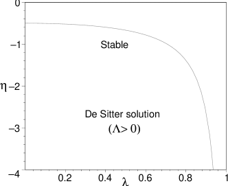
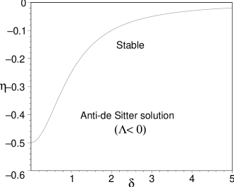
Figure 1: We have defined $\lambda=a_{0}/(3/\Lambda)^{1/2}$ and $\delta=a_{0}/(3/|\Lambda|)^{1/2}$, respectively. The regions of stability are depicted in the graphs, below the curves for the de-Sitter and the anti-de Sitter solutions, respectively.

3. Schwarzschild spacetime.

This is the particular case of the Poisson-Visser analysis Poisson , with $\Lambda=0$, which reduces to

$$\eta_{0}<-\frac{1-3M/a_{0}+3M^{2}/a_{0}^{2}}{2\left(1-2M/a\right)\left(1-3M/a_{0}\right)}\,,\qquad a_{0}>3M\,,$$ (40)

$$\eta_{0}>-\frac{1-3M/a_{0}+3M^{2}/a_{0}^{2}}{2\left(1-2M/a\right)\left(1-3M/a_{0}\right)}\,,\qquad a_{0}<3M\,.$$ (41)

The stability regions are shown in the left plot of figure $2$.

4. Schwarzschild-anti de Sitter spacetime.

For the Schwarzschild-anti de Sitter spacetime, with $\Lambda<0$, we have

$$\eta_{0}<-\frac{1-3M/a_{0}+3M^{2}/a_{0}^{2}+|\Lambda|\,Ma_{0}}{2\left(1-2M/a_{0}+|\Lambda|\,a_{0}^{2}/3\right)\left(1-3M/a_{0}\right)}\,,\qquad a_{0}>3M$$ (42)

$$\eta_{0}>-\frac{1-3M/a_{0}+3M^{2}/a_{0}^{2}+|\Lambda|\,Ma_{0}}{2\left(1-2M/a_{0}+|\Lambda|\,a_{0}^{2}/3\right)\left(1-3M/a_{0}\right)}\,,\qquad a_{0}<3M$$ (43)

The regions of stability are depicted in the right plot of figure $2$, considering the value $9|\Lambda|M^{2}=0.9$. In this case, the black hole event horizon is given by $r_{b}\simeq 1.8\,M$. We verify that the regions of stability decrease, relatively to the Schwarzschild case.

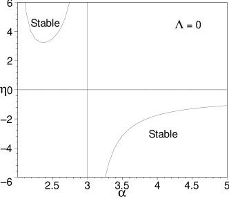
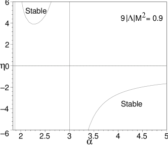
Figure 2: We have defined $\alpha=a_{0}/M$. The regions of stability are depicted for the Schwarzschild and the Schwarzschild-anti de Sitter solutions, respectively. Imposing the value $9|\Lambda|M^{2}=0.9$ in the Schwarzschild-anti de Sitter case, we verify that the stability regions decrease relatively to the Schwarzschild solution.

5. Schwarzschild-de Sitter spacetime.

For the Schwarzschild-de Sitter spacetime, with $\Lambda>0$, we have

$$\eta_{0}<-\frac{1-3M/a_{0}+3M^{2}/a_{0}^{2}-\Lambda Ma_{0}}{2\left(1-2M/a_{0}-\Lambda a_{0}^{2}/3\right)\left(1-3M/a_{0}\right)}\,,\qquad \,a_{0}>3M$$ (44)

$$\eta_{0}>-\frac{1-3M/a_{0}+3M^{2}/a_{0}^{2}-\Lambda Ma_{0}}{2\left(1-2M/a_{0}-\Lambda a_{0}^{2}/3\right)\left(1-3M/a_{0}\right)}\,,\qquad \,a_{0}<3M.$$ (45)

The regions of stability are depicted in figure $3$ for increasing values of $9\Lambda M^{2}$. In particular, for $9\Lambda M^{2}=0.7$ the black hole and cosmological horizons are given by $r_{b}\simeq 2.33\,M$ and $r_{c}=4.71\,M$, respectively. Thus, only the interval $2.33<a_{0}/M<4.71$ is taken into account, as shown in the range of the respective plot. Analogously, for $9\Lambda M^{2}=0.9$, we find $r_{b}\simeq 2.56\,M$ and $r_{c}=3.73\,M$. Therefore only the range within the interval $2.56<a_{0}/M<3.73$ corresponds to the stability regions, also shown in the respective plot.

We verify that for large values of $\Lambda$, or large $M$, the regions of stability are significantly increased, relatively to the $\Lambda=0$ case.

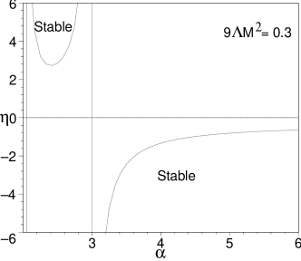
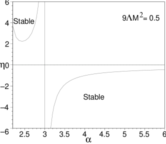
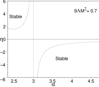
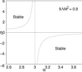
Figure 3: We have defined $\alpha=a_{0}/M$. The regions of stability for the Schwarzschild-de Sitter solution, imposing $9\Lambda M^{2}=0.3$, $9\Lambda M^{2}=0.5$, $9\Lambda M^{2}=0.7$ and $9\Lambda M^{2}=0.9$, respectively. The regions of stability are significantly increased, relatively to the $\Lambda=0$ case, for increasing values of $9\Lambda M^{2}$.

IV A thin shell around a traversable wormhole

As an alternative to the thin-shell wormhole, constructed using the cut-and-paste technique analyzed above, one may also consider that the exotic matter is distributed from the throat $r_{0}$ to a radius $a$, where the solution is matched to an exterior vacuum spacetime. Thus, the thin shell confines the exotic matter threading the wormhole to a finite region, with a delta-function distribution of the stress-energy tensor on the junction surface.

We shall match the interior wormhole solution Morris

$$ds^{2}=-e^{2\Phi(r)}\,dt^{2}+\frac{dr^{2}}{1-b(r)/r}+r^{2}\,(d\theta^{2}+\sin^{2}{\theta}\,d\phi^{2})\,,$$ (46)

to the exterior vacuum solution

$$ds^{2}=-\left(1-\frac{2M}{r}-\frac{\Lambda}{3}r^{2}\right)\,dt^{2}+\left(1-\frac{2M}{r}-\frac{\Lambda}{3}r^{2}\right)^{-1}\,dr^{2}+r^{2}\,(d\theta^{2}+\sin^{2}{\theta}\,d\phi^{2})\,,$$ (47)

at a junction surface, $\Sigma$. Thus, the intrinsic metric to $\Sigma$ is given by

$$ds^{2}_{\Sigma}=-d\tau^{2}+a^{2}\,(d\theta^{2}+\sin^{2}{\theta}\,d\phi^{2})\,.$$ (48)

Note that the junction surface, $r=a$, is situated outside the event horizon, i.e., $a>r_{b}$, to avoid a black hole solution.

Thus, using equation (3), the non-trivial components of the extrinsic curvature are given by

$$K^{\tau\;+}_{\;\;\tau} = \frac{\frac{M}{a^{2}}-\frac{\Lambda}{3}a}{\sqrt{1-\frac{2M}{a}-\frac{\Lambda}{3}a^{2}}}\;,$$ (49)

$$K^{\tau\;-}_{\;\;\tau} = \Phi^{\prime}(a)\sqrt{1-\frac{b(a)}{a}}\;,$$ (50)

and

$$K^{\theta\;+}_{\;\;\theta} = \frac{1}{a}\sqrt{1-\frac{2M}{a}-\frac{\Lambda}{3}a^{2}}\;,$$ (51)

$$K^{\theta\;-}_{\;\;\theta} = \frac{1}{a}\sqrt{1-\frac{b(a)}{a}}\;.$$ (52)

The Einstein equations, equations (9)-(10), with the extrinsic curvatures, equations (49)-(52), then provide us with the following expressions for the surface stresses

$$\sigma = -\frac{1}{4\pi a}\left(\sqrt{1-\frac{2M}{a}-\frac{\Lambda}{3}a^{2}}-\sqrt{1-\frac{b(a)}{a}}\,\right),$$ (53)

$$p = \frac{1}{8\pi a}\left(\frac{1-\frac{M}{a}-\frac{2\Lambda}{3}a^{2}}{\sqrt{1-\frac{2M}{a}-\frac{\Lambda}{3}a^{2}}}-\zeta\,\sqrt{1-\frac{b(a)}{a}}\,\right),$$ (54)

with $\zeta=1+a\Phi^{\prime}(a)$. If the surface stress-energy terms are null, the junction is denoted as a boundary surface. If surface stress terms are present, the junction is called a thin shell, which is represented in figure $4$.

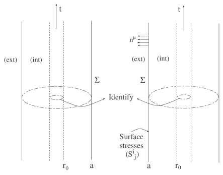
Figure 4: Two copies of static timelike hypersurfaces, $\Sigma$, embedded in asymptotic regions, separating an interior wormhole solution from an exterior vacuum spacetime. Both copies are identified at the wormhole throat, $r_{0}$. The surface stresses reside on $\Sigma$, and members of the normal vector field, $n^{\mu}$, are shown.

The surface mass of the thin shell is given by

$$M_{\rm shell}=4\pi a^{2}\sigma=a\left(\sqrt{1-\frac{b(a)}{a}}-\sqrt{1-\frac{2M}{a}-\frac{\Lambda}{3}a^{2}}\,\right).$$ (55)

One may interpret $M$ as the total mass of the system, in this case being the total mass of the wormhole in one asymptotic region. Thus, solving equation (55) for $M$, we finally have

$$M=\frac{b(a)}{2}+M_{\rm shell}\left(\sqrt{1-\frac{b(a)}{a}}-\frac{M_{\rm shell}}{2a}\right)-\frac{\Lambda}{6}a^{3}\,.$$ (56)

IV.1 Energy conditions at the junction surface

The junction surface may serve to confine the interior wormhole exotic matter to a finite region, which in principle may be made arbitrarily small, and one may impose that the surface stress-energy tensor obeys the energy conditions at the junction, $\Sigma$ VisserBOOK ; hawkingellis .

We shall only consider the weak energy condition (WEC) and the null energy condition (NEC). The WEC implies $\sigma\geq 0$ and $\sigma+p\geq 0$, and by continuity implies the null energy condition (NEC), $\sigma+p\geq 0$.

From eqs. (53)-(54), we deduce

$$\sigma+p=\frac{1}{8\pi a}\left[(2-\zeta)\,\sqrt{1-\frac{b(a)}{a}}-\frac{1-\frac{3M}{a}}{\sqrt{1-\frac{2M}{a}-\frac{\Lambda}{3}a^{2}}}\right].$$ (57)

We shall next find domains in which the NEC is satisfied, by imposing that the surface energy density is non-negative, $\sigma\geq 0$, i.e., $\sqrt{1-b(a)/a}\geq\sqrt{1-2M/a-\Lambda a^{2}/3}$.

1. Schwarzschild solution

Consider the Schwarzschild solution, $\Lambda=0$ and we impose that the surface energy density is non-negative, $\sigma\geq 0$. For the particular case of $\zeta\leq 1$, from equation (57) we verify that $\sigma+p\geq 0$ is readily satisfied for $\forall\,a$.

For $1<\zeta<2$, the NEC is verified in the following region

$$2M<a\leq 2M\,\left(\frac{\zeta-\frac{1}{2}}{\zeta-1}\right).$$ (58)

For convenience, by defining a new parameter $\xi=2M/a$, equation (58) takes the form

$$\frac{\zeta-1}{\zeta-\frac{1}{2}}\leq\xi<1\,.$$ (59)

For $\zeta=2$, the NEC is satisfied for $\xi\geq 2/3$, i.e., $a\leq 3M$. For $\zeta>2$, we need to impose the NEC in the region of equation (59); with $\sigma+p<0$ for $\xi<(\zeta-1)/(\zeta-1/2)$.

2. Schwarzschild-de Sitter solution

For the Schwarzschild-de Sitter spacetime, $\Lambda>0$, we shall once again impose a non-negative surface energy density, $\sigma\geq 0$. Consider the definitions $\beta=9\Lambda M^{2}$ and $\xi=2M/a$.

For $\zeta<2$ the condition $\sigma+p\geq 0$ is readily met for $\beta\leq\beta_{0}$, with $\beta_{0}$ given by

$$\beta_{0}=\frac{27}{4}\,\frac{\xi^{2}}{(2-\zeta)}\,\left[(1-\zeta)+\left(\zeta-\frac{1}{2}\right)\xi\right].$$ (60)

Choosing a particular example, for instance $\zeta=-0.5$, consider figure 5. The region of interest is shown below the solid line, which is given by $\beta_{r}=27\xi^{2}(1-\xi)/4$. The case of $\zeta=-0.5$ is depicted as a dashed curve, and the NEC is obeyed to the right of the latter.

For $\zeta=2$, then the NEC is verified for $\forall\,\beta$ and $\xi\geq 2/3$, i.e., $r_{b}<a\leq 3M$, with $r_{b}$ given by equation (12). This analysis is depicted in figure 5, to the right of the dashed curve, represented by $\xi=2$.

For the case of $\zeta>2$, the condition $\sigma+p\geq 0$ needs to be imposed in the region $\beta_{0}\leq\beta\leq\beta_{r}$; and $\sigma+p<0$ for $\beta<\beta_{0}$. The specific case of $\zeta=5$ is depicted as a dashed curve in figure 5. The NEC needs to be imposed to the right of the respective curve.

Figure 5: Analysis of the null energy condition for the Schwarzschild-de Sitter spacetime. We have considered the definitions $\beta=9\Lambda M^{2}$ and $\xi=2M/a$. Only the region below the solid line is of interest. We have considered specific examples, and the NEC is obeyed to the right of each respective dashed curves, $\zeta=-0.5$, $\zeta=2$ and $\zeta=5$. See text for details.

3. Schwarzschild-anti de Sitter solution

Considering the Schwarzschild-anti de Sitter spacetime, $\Lambda<0$, once again a non-negative surface energy density, $\sigma\geq 0$, is imposed. Consider the definitions $\gamma=9|\Lambda|M^{2}$ and $\xi=2M/a$.

For $\zeta\leq 1$ the condition $\sigma+p\geq 0$ is readily met for $\forall\,\gamma$ and $\forall\,\xi$. For $1<\zeta<2$, the NEC is satisfied in the region $\gamma\geq\gamma_{0}$, with $\gamma_{0}$ given by

$$\gamma_{0}=\frac{27}{4}\,\frac{\xi^{2}}{(2-\zeta)}\,\left[(1-\zeta)+\left(\zeta-\frac{1}{2}\right)\xi\right].$$ (61)

The particular case of $\zeta=1.8$ is depicted in figure 6. The region of interest is delimited by the $\xi$-axis and the area to the left of the solid curve, which is given by $\gamma_{r}=27\xi^{2}(\xi-1)/4$. Thus, the NEC is obeyed above the dashed curve represented by the value $\zeta=1.8$.

For $\zeta=2$, then $\sigma+p\geq 0$ is verified for $\forall\gamma$ and $\xi\geq 3/2$, i.e., $r_{b}<a\leq 3M$, with $r_{b}$ given by equation (14). Thus, the NEC is obeyed to the right of the dashed curve represented by $\zeta=2$, and to the left of the solid line, $\gamma_{r}$.

For the case of $\zeta>2$, the condition $\sigma+p\geq 0$ needs to be imposed in the region $\gamma_{r}\leq\gamma\leq\gamma_{0}$. The specific case of $\zeta=3$ is depicted in figure 6 as a dashed curve. Thus, the NEC needs to be imposed in the region to the right of the respective dashed curve and to the left of the solid line, $\gamma_{r}$.

Figure 6: Analysis of the null energy condition for the Schwarzschild-anti de Sitter spacetime. We have considered the definitions $\gamma=9|\Lambda|M^{2}$ and $\xi=2M/a$. The only area of interest is depicted to the left of the solid curve, given by $\gamma_{r}=27\xi^{2}(\xi-1)/4$. For the specific case of $\zeta=1.8$, the NEC is obeyed above the respective curve. For the cases of $\zeta=2$ and $\zeta=3$, the NEC is verified to the right of the respective dashed curves, and to the left of the solid line. See text for details.

IV.2 Specific cases

Taking into account equations (53)-(54), one may express $p$ as a function of $\sigma$ by the following relationship

$$p=\frac{1}{8\pi a}\,\left[\frac{(1-\zeta)+(\zeta-\frac{1}{2})\,\frac{2M}{a}-(2-\zeta)\frac{\Lambda}{3}a^{2}}{\sqrt{1-\frac{2M}{a}-\frac{\Lambda}{3}a^{2}}}-4\pi a\zeta\sigma\right].$$ (62)

We shall analyze equation (62), namely, find domains in which $p$ assumes the nature of a tangential surface pressure, $p>0$, or a tangential surface tension, $p<0$, for the Schwarzschild case, $\Lambda=0$, the Schwarzschild-de Sitter spacetime, $\Lambda>0$, and for the Schwarzschild-anti de Sitter solution, $\Lambda<0$. In the analysis that follows we shall consider that $M$ is positive, $M>0$.

1. Schwarzschild spacetime

For the Schwarzschild spacetime, $\Lambda=0$, equation (62) reduces to

$$p=\frac{1}{8\pi a}\,\left[\frac{(1-\zeta)+(\zeta-\frac{1}{2})\,\frac{2M}{a}}{\sqrt{1-\frac{2M}{a}}}-4\pi a\zeta\sigma\right]\,.$$ (63)

To find domains in which $p$ is a tangential surface pressure, $p>0$, or a tangential surface tension, $p<0$, it is convenient to express equation (63) in the following compact form

$$p=\frac{1}{16\pi M}\,\frac{\Gamma(\xi,\zeta,\mu)}{\sqrt{1-\xi}}\,,$$ (64)

with $\xi=2M/a$ and $\mu=8\pi M\sigma$. $\Gamma(\xi,\zeta,\mu)$ is defined as

$$\Gamma(\xi,\zeta,\mu)=(1-\zeta)\,\xi+\left(\zeta-\frac{1}{2}\right)\xi^{2}-\mu\zeta\sqrt{1-\xi}\;.$$ (65)

One may now fix one or several of the parameters and analyze the sign of $\Gamma(\xi,\zeta,\mu)$, and consequently the sign of $p$.

Fixed $\zeta$, varying $\xi$ and $\mu$. For instance, consider a fixed value of $\zeta$, varying the parameters $(\xi,\mu)$, i.e., consider a fixed value of $a\Phi^{\prime}(a)$ and vary the values of the junction radius, $a$, and of the surface energy density, $\sigma$. It is necessary to separate the cases of $\zeta=0$, $\zeta>0$ and $\zeta<0$, respectively.

Firstly, for the case of $\zeta=0$, equation (65) reduces to $\Gamma(\xi,\zeta=0,\mu)=\xi-\xi^{2}/2$, which is always positive, as $0<\xi<1$, implying a tangential surface pressure, $p>0$.

Secondly, for $\zeta>0$, the qualitative behavior can be represented by the specific case of $\zeta=1$, corresponding to a constant redshift function and depicted in figure 7. For non-positive values of $\mu$ and $\forall\,\xi$ a surface pressure, $p>0$, is required to hold the thin shell structure against collapse. Close to the black hole event horizon, $a\rightarrow 2M$, i.e. $\xi\rightarrow 1$, a surface pressure is also needed to hold the structure against collapse. For high values of $\mu$ and low values of $\xi$, a surface tangential tension, $p<0$, is needed to hold the structure against expansion. In particular, for the constant redshift function, $\Phi^{\prime}(r)=0$, and a null surface energy density, $\sigma=0$, i.e., $\zeta=1$ and $\mu=0$, respectively, equation (65) reduces to $\Gamma(\xi)=\xi^{2}/2$, from which we readily conclude that $p$ is non-negative everywhere, tending to zero at infinity, i.e., $\xi\rightarrow 0$. This is a particular case analyzed in LLQ . Note that a surface boundary, with $p=0$ and $\sigma=0$, is given by $\xi=(\zeta-1)/(\zeta-1/2)$, for $\zeta>1$.

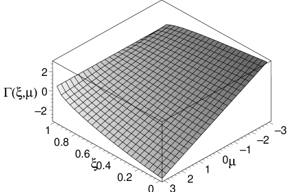
Figure 7: The surface represents the sign of $p$ for the Schwarzschild spacetime, $\Lambda=0$, with a constant redshift function, $\Phi^{\prime}(r)=0$, i.e., $\zeta=1$. For non-positive values of $\mu$ and $\forall\,\xi$, we have a surface tangential pressure, $p>0$. For extremely high values of $\xi$ (close to the black hole event horizon) and $\forall\,\mu$, a surface pressure is also required to hold the structure against collapse. For high $\mu$ and low $\xi$, we have a tangential surface tension, $p<0$. See text for details.

Finally, for the $\zeta<0$ case, the qualitative behavior can be represented by the specific case of $\zeta=-1$, depicted in figure 8. For non-negative values of $\mu$ and for $\forall\,\xi$, a surface pressure, $p>0$, is required. For low negative values of $\mu$ and for low values of $\xi$, a surface tension is needed, which is somewhat intuitive as a negative surface energy density is gravitationally repulsive, requiring a surface tension to hold the structure against expansion.

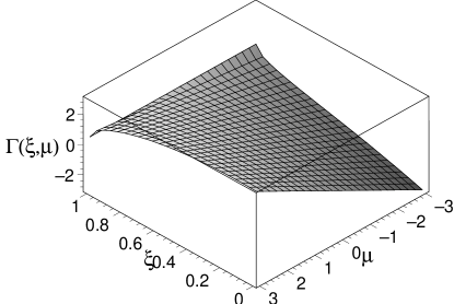
Figure 8: The surface is given by equation (65) for the Schwarzschild spacetime, $\Lambda=0$, with $\zeta=-1$. For non-negative values of $\mu$ and $\forall\,\xi$, we have a surface tangential pressure, $p>0$. For negative values of $\mu$ and low $\xi$, a tangential surface tension, $p<0$, is required to hold the structure against expansion. See text for details.

2. Schwarzschild-de Sitter spacetime

For the Schwarzschild-de Sitter spacetime with $\Lambda>0$, to analyze the sign of $p$, it is convenient to express equation(62) in the following compact form

$$p=\frac{1}{16\pi M}\,\frac{\Gamma(\xi,\zeta,\mu,\beta)}{\sqrt{1-\xi-\frac{4\beta}{27\xi^{2}}}}\,,$$ (66)

with $\xi=2M/a$, $\mu=8\pi M\sigma$ and $\beta=9\Lambda M^{2}$. $\Gamma(\xi,\zeta,\mu,\beta)$ is defined as

$$\Gamma(\xi,\zeta,\mu,\beta)=(1-\zeta)\,\xi+\left(\zeta-\frac{1}{2}\right)\xi^{2}-\frac{4\beta}{27\xi}\,(2-\zeta)-\mu\zeta\sqrt{1-\xi-\frac{4\beta}{27\xi^{2}}}\;.$$ (67)

One may now fix several of the parameters and analyze the sign of $\Gamma(\xi,\zeta,\mu,\beta)$, and consequently the sign of $p$.

Null surface energy density. For instance, consider a null surface energy density, $\sigma=0$, i.e., $\mu=0$. Thus, equation (67) reduces to

$$\Gamma(\xi,\zeta,\beta)=(1-\zeta)\,\xi+\left(\zeta-\frac{1}{2}\right)\,\xi^{2}-(2-\zeta)\,\frac{4\beta}{27\xi}\,.$$ (68)

To analyze the sign of $p$, we shall consider a null tangential surface pressure, i.e., $\Gamma(\xi,\zeta,\beta)=0$, so that from equation (68) we have the following relationship

$$\beta_{0}=\frac{27}{4}\frac{\xi^{2}}{(2-\zeta)}\left[(1-\zeta)+\left(\zeta-\frac{1}{2}\right)\,\xi\right]\,,$$ (69)

with $\zeta\neq 2$, which is identical to equation (60).

For the particular case of $\zeta=2$, from equation (68), we have $\Gamma(\xi,\zeta=2,\beta)=\xi(3\xi/2-1)$. A surface boundary, $\Gamma(\xi,\zeta=2,\beta)=0$, is presented at $\xi=2/3$, i.e., $a=3M$. A surface pressure, $\Gamma(\xi,\zeta=2,\beta)>0$, is given for $\xi>2/3$, i.e., $r_{b}<a<3M$, and a surface tension, $\Gamma(\xi,\zeta=2,\beta)<0$, for $\xi<2/3$, i.e., $3M<a<r_{c}$.

For $\zeta<2$, from equation (68), a surface pressure, $\Gamma(\xi,\zeta,\beta)>0$, is met for $\beta<\beta_{0}$, and a surface tension, $\Gamma(\xi,\zeta,\beta)<0$, for $\beta>\beta_{0}$. The specific case of a constant redshift function, i.e., $\zeta=1$, is analyzed in LLQ (For this case, equation (69) is reduced to $\beta_{0}=27\xi^{3}/8$, or $M=\Lambda a^{3}/3$). For the qualitative behavior, the reader is referred to the particular case of $\zeta=-0.5$ provided in Fig. 5. To the right of the curve a surface pressure, $p>0$, is given and to the left of the respective curve a surface tension, $p<0$.

For $\zeta>2$, from equation (68), a surface pressure, $\Gamma(\xi,\zeta,\beta)>0$, is given for $\beta_{0}<\beta<\beta_{r}$, and a surface tension, $\Gamma(\xi,\zeta,\beta)<0$, for $\beta<\beta_{0}$. Once again the reader is referred to fig. 5 for a qualitative analysis of the behavior for the particular case of $\zeta=5$. A surface pressure is given to the right of the curve and a surface tension to the left.

Note that for the analysis considered in this section, namely, for a null surface energy density, the WEC, and consequently the NEC, are satisfied only if $p\geq 0$. The results obtained are consistent with those of the section regarding the energy conditions at the junction surface, for the Schwarzschild-de Sitter spacetime, considered above.

3. Schwarzschild-anti de Sitter spacetime

For the Schwarzschild-anti de Sitter spacetime, $\Lambda<0$, to analyze the sign of $p$, equation (62) is expressed as

$$p=\frac{1}{16\pi M}\,\frac{\Gamma(\xi,\zeta,\mu,\gamma)}{\sqrt{1-\xi+\frac{4\gamma}{27\xi^{2}}}}\,,$$ (70)

with the parameters given $\xi=2M/a$, $\mu=8\pi M\sigma$ and $\gamma=9|\Lambda|M^{2}$, respectively. $\Gamma(\xi,\zeta,\mu,\gamma)$ is defined as

$$\Gamma(\xi,\zeta,\mu,\gamma)=(1-\zeta)\,\xi+\left(\zeta-\frac{1}{2}\right)\xi^{2}+\frac{4\gamma}{27\xi}\,(2-\zeta)-\mu\zeta\sqrt{1-\xi+\frac{4\gamma}{27\xi^{2}}}\;.$$ (71)

As in the Schwarzschild-de Sitter solution we shall analyze the case of a null surface energy density, $\sigma=0$, i.e., $\mu=0$.

Null surface energy density. For a null surface energy density, $\sigma=0$, i.e., $\mu=0$, equation (71) reduces to

$$\Gamma(\xi,\zeta,\gamma)=(1-\zeta)\,\xi+\left(\zeta-\frac{1}{2}\right)\,\xi^{2}+(2-\zeta)\,\frac{4\gamma}{27\xi}\,,$$ (72)

To analyze the sign of $p$, once again we shall consider a null tangential surface pressure, i.e., $\Gamma(\xi,\zeta,\beta)=0$, so that from equation (72) we have

$$\gamma_{0}=\frac{27}{4}\frac{\xi^{2}}{(2-\zeta)}\left[(\zeta-1)-\left(\zeta-\frac{1}{2}\right)\,\xi\right]\,,$$ (73)

with $\zeta\neq 2$, which is identical to equation (61).

For the particular case of $\zeta=2$, from equation (72), we have $\Gamma(\xi,\zeta=2,\beta)=\xi(3\xi/2-1)$, which is null at $\xi=2/3$, i.e., $a=3M$. A surface pressure, $\Gamma(\xi,\zeta=2,\gamma)>0$, is given for $\xi>2/3$, i.e., $r_{b}<a<3M$, and a surface tension, $\Gamma(\xi,\zeta=2,\beta)<0$, for $\xi<2/3$, i.e., $a>3M$. The reader is referred to the particular case of $\zeta=2$, depicted in figure 6. A surface pressure is given to the right of the respective dashed curve, and a surface tension to the left.

For $\zeta\leq 1$, a surface pressure, $\Gamma(\xi,\zeta,\gamma)>0$, is given for $\forall\;\gamma$ and $\forall\;\xi$. For $1<\zeta<2$, a surface pressure, $\Gamma(\xi,\zeta,\gamma)>0$, is given for $\gamma>\gamma_{0}>0$; and a surface tension, $\Gamma(\xi,\zeta,\gamma)<0$, is provided for $0<\gamma<\gamma_{0}$. The particular case of $\zeta=1.8$ is depicted in figure 6, in which a surface pressure is presented above the respective dashed curve, and a surface tension is presented in the region delimited by the curve and the $\xi$-axis.

For $\zeta>2$, a surface pressure, $\Gamma(\xi,\zeta,\gamma)>0$, is met for $\gamma_{r}<\gamma<\gamma_{0}$, and a surface tension, $\Gamma(\xi,\zeta,\gamma)<0$, for $\gamma>\gamma_{0}$. The specific case for $\zeta=3$ is depicted in figure 6. A surface pressure is presented to the right of the respective curve, and a surface tension to the left.

Once again, the analysis considered in this section is consistent with the results obtained in the section regarding the energy conditions at the junction surface, for the Schwarzschild-anti de Sitter spacetime, considered above. This is due to the fact that for the specific case of a null surface energy density, the regions in which the WEC and NEC are satisfied coincide with the range of $p\geq 0$.

IV.3 Pressure balance equation

One may obtain an equation governing the behavior of the radial pressure in terms of the surface stresses at the junction boundary from the following identity VisserBOOK ; Musgrave : $\left[\,T^{\rm total}_{\hat{\mu}\hat{\nu}}\,n^{\hat{\mu}}n^{\hat{\nu}}\right]=\frac{1}{2}(K^{i\;+}_{\;\,j}+K^{i\;-}_{\;\,j})\,S^{j}_{\;\,i}$, where $T^{\rm total}_{\hat{\mu}\hat{\nu}}=T_{\hat{\mu}\hat{\nu}}-g_{\hat{\mu}\hat{\nu}}\,\Lambda/8\pi$ is the total stress-energy tensor, and the square brackets denotes the discontinuity across the thin shell, i.e., $[X]=X^{+}|_{\Sigma}-X^{-}|_{\Sigma}$. Taking into account the values of the extrinsic curvatures, eqs. (49)-(52), and noting that the tension acting on the shell is by definition the normal component of the stress-energy tensor, $-\tau=T_{\hat{\mu}\hat{\nu}}\,n^{\hat{\mu}}n^{\hat{\nu}}$, we finally have the following pressure balance equation

$$\left(-\tau^{+}(a)-\frac{\Lambda^{+}}{8\pi}\right)-\left(-\tau^{-}(a)-\frac{\Lambda^{-}}{8\pi}\right) = \frac{1}{a}\,\left(\sqrt{1-\frac{2M}{a}-\frac{\Lambda}{3}a^{2}}+\sqrt{1-\frac{b(a)}{a}}\;\right)\,p$$ (74)

$$-\left(\frac{\frac{M}{a^{2}}-\frac{\Lambda}{3}a}{\sqrt{1-\frac{2M}{a}-\frac{\Lambda}{3}a^{2}}}+\Phi^{\prime}(a)\,\sqrt{1-\frac{b(a)}{a}}\right)\frac{\sigma}{2},$$

where the $\pm$ superscripts correspond to the exterior and interior spacetimes, respectively. Equation (74) relates the difference of the radial tension across the shell in terms of a combination of the surface stresses, $\sigma$ and $p$, given by eqs. (53)-(54), respectively, and the geometrical quantities.

Note that for the exterior vacuum solution we have $\tau^{+}=0$. For the particular case of a null surface energy density, $\sigma=0$, and considering that the interior and exterior cosmological constants are equal, $\Lambda^{-}=\Lambda^{+}$, equation (74) reduces to

$$\tau^{-}(a)=\frac{2}{a}\,\sqrt{1-\frac{2M}{a}-\frac{\Lambda}{3}a^{2}}\;\,p\,.$$ (75)

For a radial tension, $\tau^{-}(a)>0$, acting on the shell from the interior, a tangential surface pressure, $p>0$, is needed to hold the thin shell form collapsing. For a radial interior pressure, $\tau^{-}(a)<0$, then a tangential surface tension, $p<0$, is needed to hold the structure form expansion.

IV.4 Traversability conditions

In this section we shall consider the traversability conditions required for the traversal of a human being through the wormhole, and consequently determine specific dimensions for the wormhole. Specific cases for the traversal time and velocity will also be estimated.

Consider the redshift function given by $\Phi(r)=kr^{\alpha}$, with $\alpha,k\in\mathbb{R}$. Thus, from the definition of $\zeta=1+a\Phi^{\prime}(a)$, the redshift function, in terms of $\zeta$, takes the following form

$$\Phi(r)=\frac{\zeta-1}{\alpha}\,\left(\frac{r}{a}\right)^{\alpha},$$ (76)

with $\alpha\neq 0$. With this choice of $\Phi(r)$, $\zeta$ may also be defined as $\zeta=1+\alpha\Phi(a)$. The case of $\alpha=0$ corresponds to the constant redshift function, so that $\zeta=1$. If $\alpha<0$, then $\Phi(r)$ is finite throughout spacetime and in the absence of an exterior solution we have $\lim_{r\rightarrow\infty}\Phi(r)\rightarrow 0$. As we are considering a matching of an interior solution with an exterior solution at $a$, then it is also possible to consider the $\alpha>0$ case, imposing that $\Phi(r)$ is finite in the interval $r_{0}\leq r\leq a$.

One of the traversability conditions was that the acceleration felt by the traveller should not exceed Earth’s gravity Morris . Consider an orthonormal basis of the traveller’s proper reference frame, $({\bf e}_{\hat{0}^{\prime}},{\bf e}_{\hat{1}^{\prime}},{\bf e}_{\hat{2}^{\prime}},{\bf e}_{\hat{3}^{\prime}})$, given in terms of the orthonormal basis of the static observers, by a Lorentz transformation. The traveller’s four-acceleration expressed in his proper reference frame, $a^{\hat{\mu}^{\prime}}=U^{\hat{\nu}^{\prime}}U^{\hat{\mu}^{\prime}}_{\;\;\;;\hat{\nu}^{\prime}}$, yields the following restriction

$$\Bigg{|}\left(1-\frac{b}{r}\right)^{1/2}\;e^{-\Phi}\,(\gamma e^{\Phi})^{\prime}\,c^{2}\Bigg{|}\leq g_{\oplus}\,,$$ (77)

where $\gamma=(1-v^{2})^{1/2}$, and $v$ being the velocity of the traveller Morris . The condition is immediately satisfied at the throat, $r_{0}$. From equation (77), one may also find an estimate for the junction surface, $a$. Considering that $(1-b(a)/a)^{1/2}\approx 1$ and $\gamma\approx 1$, i.e., for low traversal velocities, and taking into account equation (76), from equation (77) one deduces $a\geq|\zeta-1|c^{2}/g_{\oplus}$. Considering the equality case, one has

$$a=\frac{|\zeta-1|c^{2}}{g_{\oplus}}\,.$$ (78)

Providing a value for $|\zeta-1|$, one may find an estimate for $a$. For instance, considering that $|\zeta-1|\simeq 10^{-10}$, one finds that $a\approx 10^{6}\,{\rm m}$.

Another of the traversability conditions that was required, was that the tidal accelerations felt by the traveller should not exceed the Earth’s gravitational acceleration. The tidal acceleration felt by the traveller is given by $\Delta a^{\hat{\mu}^{\prime}}=-R^{\hat{\mu}^{\prime}}_{\;\;\hat{\nu}^{\prime}\hat{\alpha}^{\prime}\hat{\beta}^{\prime}}\,U^{\hat{\nu}^{\prime}}\eta^{\hat{\alpha}^{\prime}}U^{\hat{\beta}^{\prime}}$, where $U^{\hat{\mu}^{\prime}}$ is the traveller’s four velocity and $\eta^{\hat{\alpha}^{\prime}}$ is the separation between two arbitrary parts of his body. For simplicity, we shall assume that $|\eta^{\hat{\alpha}^{\prime}}|\approx 2\,{\rm m}$ along any spatial direction in the traveller’s reference frame, and that $|\Delta a^{\hat{\mu}^{\prime}}|\leq g_{\oplus}$. Consider the radial tidal constraint, $|R_{\hat{1}^{\prime}\hat{0}^{\prime}\hat{1}^{\prime}\hat{0}^{\prime}}|=|R_{\hat{r}\hat{t}\hat{r}\hat{t}}|\leq g_{\oplus}/2c^{2}$, which can be regarded as constraining the metric field $\Phi(r)$, i.e.,

$$\Bigg{|}\left(1-\frac{b}{r}\right)\left(-\Phi^{\prime\prime}+\frac{b^{\prime}r-b}{2r(r-b)}\,\Phi^{\prime}-(\Phi^{\prime})^{2}\right)\Bigg{|}\leq\frac{g_{\oplus}}{2c^{2}}\,.$$ (79)

At the throat, $r=r_{0}$, and taking into account equation (76), then equation (79) reduces to $|(b^{\prime}-1)\Phi^{\prime}(r_{0})/2r_{0}|\leq g_{\oplus}/2c^{2}$ or

$$a=\left(\frac{|b^{\prime}-1|\,|\zeta-1|c^{2}}{g_{\oplus}r_{0}^{2}}\right)^{1/\alpha}\;r_{0}\,.$$ (80)

considering the equality case.

Using eqs. (78) and (80), one may find an estimate for the throat radius, by providing a specific value for $\alpha$. Considering $\alpha=-1$ and equating eqs. (78) and (80), one finds

$$r_{0}=\left(\frac{|b^{\prime}-1|\,|\zeta-1|^{2}\,c^{4}}{g_{\oplus}^{2}}\right)^{1/3}\,.$$ (81)

Kuhfittig Kuhfittig ; Kuhfittig2 ; Kuhfittig3 proposed models restricting the exotic matter to an arbitrarily thin region under the condition that $b^{\prime}(r)$ be close to unity near the throat. If $b^{\prime}(r_{0})\approx 1$, then the embedding diagram will flare out very slowly, so that from equation (81), $r_{0}$ may be made arbitrarily small. Nevertheless, using the form functions specified in Morris we will consider that $|b^{\prime}-1|\approx 1$. Using the above value of $|\zeta-1|=10^{-10}$, then from equation (81) we find $r_{0}\simeq 10^{4}\,{\rm m}$.

To determine the traversal time of the total trip, suppose that the traveller accelerates at $g_{\oplus}$ halfway to the throat, then decelerates at the same rate coming to rest at the throat Morris ; Kuhfittig2 . For simplicity, we shall consider $b^{\prime}\approx 1$ near the throat, so the the wormhole will flare out very slowly. Therefore, from Eq. (81) the throat will be relatively small, so that we may assume that $r_{0}\approx 0$, as in Kuhfittig2 . Consider that a space station is situated just outside the junction surface at $a$, from which the intrepid traveller will start his/her journey. Thus, the total time of the trip will be approximately $t_{\rm total}\simeq 4\sqrt{2a/g_{\oplus}}\approx 1800\,{\rm s}=30\,{\rm min}$. The maximum velocity attained by the traveller will be approximately $v_{{\rm max}}\simeq 4.5\,{\rm km/s}$.

V Conclusion

By using the cut-and-paste technique we have constructed thin-shell wormholes in the presence of a generic cosmological constant. Applying a linearized stability analysis we have found that for large positive values of $\Lambda$, i.e., the Schwarzschild-de Sitter solution, the regions of stability significantly increase relatively to the Schwarzschild case, analyzed by Poisson and Visser. For negative values of $\Lambda$, i.e., the Schwarzschild-anti de Sitter, the regions of stability decrease.

We have also constructed solutions by matching an interior wormhole spacetime to a vacuum exterior solution at a junction surface situated at $a$. We have been interested in analyzing the domains in which the weak and null energy conditions are satisfied at the junction surface, in the spirit of minimizing the usage of exotic matter. The characteristics and several physical properties of the surface stresses were explored, namely, regions where the sign of tangential surface pressure is positive and negative (surface tension) were specified. An equation governing the behavior of the radial pressure across the junction surface was deduced. Specific dimensions of the wormhole, namely, the throat radius and the junction interface radius, were found taking into account the traversability conditions, and estimates for the traversal time and velocity were also studied.

- (1) M. Morris and K.S. Thorne, “Wormholes in spacetime and their use for interstellar travel: A tool for teaching General Relativity”, Am. J. Phys. 56, 395 (1988).
- (2) M. Visser, Lorentzian Wormholes: From Einstein to Hawking (American Institute of Physics, New York, 1995).
- (3) C. Barcelo and M. Visser, “Twilight for the energy conditions?”, Int. J. Mod. Phys. D 11, 1553 (2002).
- (4) M. Visser, “General overview of chronology protection”, talk delivered at the APCTP Winter School and Workshop: Quantum Gravity, Black Holes and Wormholes, POSTECH, Pohang School of Environmental Engineering, South Korea, 11-14 Dec. 2003.
- (5) For a review, see for instance (and references therein): F. Lobo and P. Crawford, “Time, Closed Timelike Curves and Causality”, The Nature of Time: Geometry, Physics and Perception, NATO Science Series II. Mathematics, Physics and Chemistry - Vol. 95, Kluwer Academic Publishers, R. Buccheri et al. eds, pp.289-296 (2003).
- (6) For a review article, see for example: F. Lobo and P. Crawford, “Weak energy condition violation and superluminal travel”, Current Trends in Relativistic Astrophysics, Theoretical, Numerical, Observational, Lecture Notes in Physics 617, Springer-Verlag Publishers, L. Fern ndez et al. eds, pp.277-291 (2003).
- (7) M. Visser, “Traversable wormholes: Some simple examples”, Phys. Rev. D 39, 3182 (1989).
- (8) M. Visser, “Traversable wormholes from surgically modified Schwarzschild spacetimes”, Nucl. Phys. B328, 203 (1989).
- (9) G. Darmois, “Mémorial des sciences mathématiques XXV”, Fasticule XXV ch V (Gauthier-Villars, Paris, France, 1927).
- (10) W. Israel, “Singular hypersurfaces and thin shells in general relativity”, Nuovo Cimento 44B, 1 (1966); and corrections in ibid. 48B, 463 (1966).
- (11) A. Papapetrou and A. Hamoui, “Couches simple de matière en relativité générale”, Ann. Inst. Henri Poincaré 9, 179 (1968).
- (12) S. W. Kim, “Schwarzschild-de Sitter type wormhole”, Phys. Lett. A 166, 13 (1992).
- (13) M. Visser, Phys. Lett. B 242, 24 (1990).
- (14) S. W. Kim, H. Lee, S. K. Kim and J. Yang, “(2+1)-dimensional Schwarzschild-de Sitter wormhole”, Phys. Lett. A 183, 359 (1993).
- (15) E. Poisson and M. Visser, “Thin-shell wormholes: Linearization stability”, Phys. Rev. D 52 7318 (1995).
- (16) F. S. N. Lobo and P. Crawford, “Linearized stability analysis of thin-shell wormholes with a cosmological constant”, Class. Quant. Grav. 21, 391 (2004).
- (17) M. Visser, S. Kar and N. Dadhich, “Traversable wormholes with arbitrarily small energy condition violations”, Phys. Rev. Lett. 90, 201102 (2003).
- (18) M. Visser, “Wormholes with infinitesimal energy condition violations”, talk delivered at the APCTP Winter School and Workshop: Quantum Gravity, Black Holes and Wormholes, POSTECH, Pohang School of Environmental Engineering, South Korea, 11-14 Dec. 2003.
- (19) F. S. N. Lobo, “Surface stresses on a thin shell surrounding a spherically symmetric traversable wormhole”, (In preparation).
- (20) J. P. S. Lemos, F. S. N. Lobo and S. Q. de Oliveira, “Morris-Thorne wormholes with a cosmological constant”, Phys. Rev. D 68, 064004 (2003).
- (21) J. P. S. Lemos and F. S. N. Lobo, “Plane symmetric traversable wormholes in an anti-de Sitter background”, (Submitted for publication).
- (22) J. P. S. Lemos, “Gravitational collapse to toroidal, cylindrical and planar black holes”, Phys. Rev. D 57, 4600 (1998).
- (23) J. P. S. Lemos, “Two-dimensional black holes and planar General Relativity”, Class. Quant. Grav. 12, 1081 (1995).
- (24) J. P. S. Lemos, “Three-dimensional black holes and cylindrical General Relativity”, Phys. Lett. B352, 46 (1995).
- (25) J. P. S. Lemos and V. T. Zanchin, “Charged Rotating Black Strings and Three Dimensional Black Holes”, Phys. Rev. D 54, 3840 (1996).
- (26) S. W. Hawking and G.F.R. Ellis, The Large Scale Structure of Spacetime, (Cambridge University Press, Cambridge 1973).
- (27) P. Musgrave and K. Lake, “Junctions and thin shells in general relativity using computer algebra I: The Darmois-Israel Formalism”, Class.Quant.Grav. 13 1885 (1996).
- (28) P. K. F. Kuhfittig, “A wormhole with a special shape function”, Am. J. Phys. 67, 125 (1999).
- (29) P. K. F. Kuhfittig, “Static and dynamic traversable wormhole geometries stisfying the Ford-Roman constraints”, Phys. Rev. D 66, 024015 (2002).
- (30) P. K. F. Kuhfittig, “Can a wormhole supported by only small amounts of exotic matter really be traversable?”, Phys. Rev. D 68, 067502 (2003).