Highly Damped Quasinormal Modes of Kerr Black Holes:
A Complete Numerical Investigation
Abstract
We compute for the first time very highly damped quasinormal modes of the (rotating) Kerr black hole. Our numerical technique is based on a decoupling of the radial and angular equations, performed using a large-frequency expansion for the angular separation constant . This allows us to go much further in overtone number than ever before. We find that the real part of the quasinormal frequencies approaches a non-zero constant value which does not depend on the spin of the perturbing field and on the angular index : . We numerically compute . Leading-order corrections to the asymptotic frequency are likely to be . The imaginary part grows without bound, the spacing between consecutive modes being a monotonic function of .
pacs:
04.70.-s, 04.30.Nk, 04.70.Bw, 11.25.-wI Introduction
Black holes (BHs), as many other objects, have characteristic vibration modes, called quasinormal modes (QNMs). The associated complex quasinormal frequencies (QN frequencies) depend only on the BH fundamental parameters: mass, charge and angular momentum. QNMs are excited by BH perturbations (as induced, for example, by infalling matter). The early evolution of a generic perturbation can be described as a superposition of QNMs, and the characteristics of gravitational radiation emitted by BHs are intimately connected to their QNM spectrum. One may in fact infer the BH parameters by observing the gravitational wave signal impinging on the detectors echeverria : this makes QNMs highly relevant in the newly born gravitational wave astronomy schutz ; kokkotas .
Besides this “classical” context, QNMs may find a very important place in the realm of a quantum theory of gravity. General semi-classical arguments suggest bekenstein that on quantizing the BH area one gets an evenly spaced spectrum of the form
| (1) |
where is the Planck length, and is an integer to be determined. Hod hod proposed to fix the value of , and therefore the area spectrum, by promoting QN frequencies with a very large imaginary part to a special position: they should bridge the gap between classical and quantum transitions. Hod obtained, for the Schwarzschild BH, . Following his proposal, further enhanced by the prospect of using similar reasoning in Loop Quantum Gravity to fix the Barbero-Immirzi parameter dreyer , the interest in highly damped BH QNMs has grown considerably cardosolemosshijun . There is now reason to believe that the connection between QN frequencies and the BH area quantum is not as straightforward as initially suggested. However a relation between classical and quantum BH properties does seem to exist, even in non-asymptotically flat spacetimes carlip . A prerequisite to study this connection is to compute QN frequencies having very large imaginary part. So far this problem has been solved only for a few special geometries: Schwarzschild BHs nollert ; motl1 ; motl2 ; andersson ; bertikerr1 , Reissner-Nordström (RN) BHs motl2 ; bertikerr1 ; andersson , the Bañados-Teitelboim-Zanelli BH cardosobtz , and the four-dimensional Schwarzschild-anti-de Sitter BH cardosoroman .
We must try to include the Kerr geometry in this short catalogue, due to its great importance and simplicity. This is a problem of great relevance for the scientific community, and quite a lot of effort is being invested here. This effort is in direct proportion to the difficulty of the problem. All previous attempts kerranalytical ; hisashi ; bertikerr1 ; bertikerr2 at probing the asymptotic QNMs of Kerr BHs have been unsuccessful, or at least unsatisfactory. There have been several contradictory “analytical” results, which were either based on incorrect assumptions, or could not probe the highly damped regime kerranalytical . The few numerical results hisashi ; bertikerr1 ; bertikerr2 are not decisive either, although they definitely show some trend. A numerical investigation is necessary both as a benchmark and as a guide to analytical approaches. Here we carry out such a numerical study. We improve on previous results by going further in overtone number than ever before, in order to really probe the asymptotic regime. The starting point for our analysis is, as previously bertikerr1 ; bertikerr2 , Leaver’s continued fraction technique leaver as improved by Nollert nollert , with a few appropriate modifications bertikerr1 . However, we now decouple the angular and radial equations. We first determine the asymptotic expansion for the angular separation constant, and then replace this asymptotic expansion in the radial equations. This trick spares us the need to solve simultaneously the two equations, which was the major drawback of previous numerical works. A leading-order asymptotic expansion of the separation constant is typically accurate for , where is the dimensionless Kerr rotation parameter conventions . In this study we go well beyond this regime (we can usually compute modes up to , an order of magnitude larger). So we have great confidence that our results really yield “asymptotic” QN frequencies.
We find that our previous results bertikerr2 for negative and moderately damped QN frequencies were quite close to the true asymptotic behaviour (especially for large values of ), while convergence to the asymptotic value was not yet achieved for positive . Our improved calculations have been carried out with two independent numerical codes. Our main results are that: (i) The real part of the QN frequencies approaches a non-zero constant value. This value does not depend on the spin of the perturbing field and on the angular index . It only depends on the rotation parameter , and is proportional to : . We determine numerically. A fit of our numerical data by power series in and suggests that leading-order corrections to the asymptotic frequency should be of order . (ii) The imaginary part grows without bound, the spacing between modes being a monotonically increasing function of .
II Basic Equations
In the Kerr geometry, the condition that a given frequency be a QN frequency can be converted into a statement about continued fractions, which is rather easy to implement numerically. Such a procedure has been explained thoroughly by Leaver leaver , so here we shall only recall the basic idea. The perturbation problem reduces to a pair of coupled differential equations: one for the angular part of the perturbations, and the other for the radial part. In Boyer-Lindquist coordinates, defining , the angular equation reads
and the radial one is
| (3) |
where and
| (4) |
The parameter for scalar, electromagnetic and gravitational perturbations respectively, and is an angular separation constant. In the Schwarzschild limit the angular separation constant can be determined analytically: .
Boundary conditions for the two equations can be cast as a couple of three-term continued fraction relations leaver . Finding QN frequencies is a two-step procedure: for assigned values of and , first find the angular separation constant looking for zeros of the angular continued fraction; then replace the corresponding eigenvalue into the radial continued fraction, and look for its zeros as a function of . This has been the strategy adopted in earlier works bertikerr1 ; bertikerr2 ; hisashi ; leaver , where the first modes were computed. These numerical investigations showed a rich (and perhaps confusing) behavior. For negative and large enough the first modes display some kind of convergence, and are consistent with our new results. Among modes with positive , only those having seemed to converge. This convergence was deceiving: positive- results in bertikerr2 were not yet in the asymptotic regime. The “true” asymptotic behavior turns out to be much simpler than the intermediate-damping regime explored in bertikerr2 .
Since the major numerical difficulty lies in the coupling of the two continued fractions, here we adopt a “trick” to decouple them. We first carry out a careful study of the angular equation, determining the asymptotic form of the separation constant for frequencies with large imaginary part. Then we substitute this expansion in Eqs. (3)-(4). By this trick we reduce the problem to the numerical solution of a single three-term recursion relation: it is then possible to probe the asymptotic regime for highly damped modes. In the following section we shall briefly discuss our main analytical and numerical results for the asymptotic expansion of .

III Asymptotic expansion of the angular separation constant
The analytical properties of the angular equation (II) and of its eigenvalues have been studied by many authors flammer ; early ; seidel ; breuerbook ; breuer . Series expansions of for are available, and they agree well with numerical results seidel . On the other hand, the asymptotic behavior for large frequencies has hardly been studied at all. An analytical power-series expansion for large (pure real and pure imaginary) values of can be found in Flammer’s book flammer , but it is limited to the case . Flammer’s results are in good agreement with the exhaustive numerical work by Oguchi oguchi , who computed angular eigenvalues for complex values of and . A review of numerical methods to compute eigenvalues and eigenfunctions for can be found in li . Quite surprisingly, there are no systematic numerical results for general spin , and the few analytical predictions for large values of do not agree with each other comment . Here we shall fill this gap, presenting some results for the large- expansion of .
A straightforward generalization of Flammer’s method can be easily found for general . Define a new angular wavefunction through breuerbook
| (5) |
and change independent variable by defining , where . Substitute this in (II) to get:
| (6) | |||||
When , this equation becomes a parabolic cylinder function. The arguments presented in flammer ; breuerbook ; breuer lead to
| (7) |
where is the number of zeros of the angular wavefunction inside the domain. One can show that
| (8) |
Higher order corrections in the asymptotic expansion can be obtained as indicated in flammer . However, we will not need them here. We have verified Eq. (7) numerically, solving Leaver’s angular continued fraction for as a function of the complex parameter . Our numerical results (which will be presented in detail elsewhere) are in excellent agreement with previous work flammer ; oguchi ; li for . For any they are consistent with equation (7) when and is large.
IV Numerical results
To compute the asymptotic QN frequencies of the Kerr black hole we use a technique similar to that described in nollert . We fix a value of the rotation parameter . We first compute QN frequencies for which , so that formula (7) is only marginally valid. This procedure is consistent with our previous intermediate-damping calculations: for example, when we include terms up to order in the asymptotic expansion for provided in flammer , our new results for and match the results for the scalar case presented in bertikerr2 at overtone numbers . Then we increase the overtone index (progressively increasing the inversion index of our “decoupled” continued fraction). Finally, we fit our numerical results by functional relations of the form:
where or . At variance with the non-rotating case nollert , fits in powers of perform better, especially for small and large . However, both fits break down as : the values of higher-order fitting coefficients increase in this limit, so that subdominant terms become as important as the leading order, and the extraction of the asymptotic frequency becomes problematic. The numerical behavior of subdominant coefficients supports the expectation (which has not yet been verified analytically) that subdominant corrections are -dependent. Therefore one has to be careful to the order in which the limits , are taken motl2 ; bertikerr1 ; bertikerr2 . These observations are consistent with the fact that, in the RN case, the zero-charge limit of the asymptotic QN frequency spectrum does not yield the asymptotic Schwarzschild QN spectrum motl2 ; andersson ; bertikerr1 .
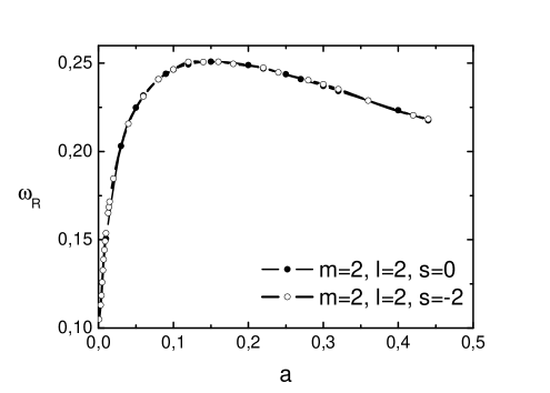
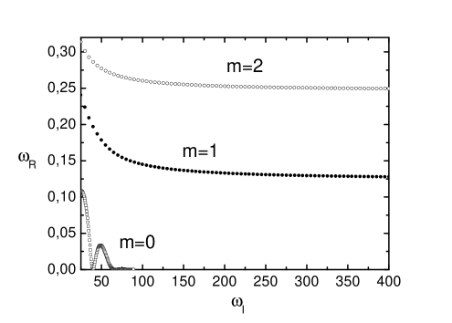
We have extracted asymptotic frequencies using two independent numerical codes. For each value of , we found that the extrapolated value of is independent of (Fig. 1), independent of and proportional to (Fig. 2): .
We obtained computing QN frequencies both for scalar perturbations () and for gravitational perturbations (). For definiteness, in both cases we picked . The agreement between the extrapolated behaviors of as a function of is excellent, suggesting that both sets of results are typically reliable with an error . Our results are also weakly dependent on the number of terms used in the asymptotic expansion of : this provides another powerful consistency check. We have tried to fit the resulting “universal function”, displayed in Fig. 3, by simple polynomials in the BH’s Hawking temperature and angular velocity (and their inverses). None of these fits reproduces our numbers with satisfactory accuracy. It is quite likely that asymptotic QN frequencies will be given by an implicit formula involving the exponential of the Kerr black hole temperature, as in the RN case motl2 ; andersson ; bertikerr1 .
For any , the imaginary part grows without bound. Quite surprisingly, the spacing between modes is a monotonically increasing function of : it is not simply given by , as recent calculations and previous numerical results suggested bertikerr1 ; spacing . A power fit in of our numerical results yields:
| (9) |
V conclusions
Motivated by recent suggestions of a link between classical black hole oscillations and quantum gravity, we have computed for the first time very highly damped QNMs of the Kerr black hole. Our calculation was made possible by a decoupling of the radial and angular equations, carried out using asymptotic expansions of the angular separation constant for and . Our results are very weakly dependent on the number of terms used in the asymptotic expansion of , and this provides a powerful consistency check. We found that:
(i) The real part of the QN frequencies approaches a non-zero constant value. This value does not depend on the spin of the perturbing field and on the angular index . It only depends on the rotation parameter , and is proportional to :
| (10) |
We determined numerically (Fig. 3), and showed that it is not given by simple polynomial functions of the black hole temperature and angular velocity (or their inverses). At fixed , a fit of our numerical data by power series in and suggests that leading-order corrections to the asymptotic frequency are probably of order . (ii) The imaginary part grows without bound, the spacing between modes being a monotonically increasing function of .
We wish to stress, once again, that the asymptotic frequency is independent on the spin of the perturbing field: this is consistent with results for highly damped QNMs of (charged) RN black holes motl2 ; andersson .
By now it is quite clear that the original Hod proposal requires some modification. However, the “universality” of the asymptotic Kerr behaviour we established in this paper is good news. For both charged and rotating black holes the asymptotic QNM frequency depends only on the black hole geometry, not on the perturbing field. If QNMs do indeed play a role in black hole quantization this is an essential prerequisite, and it seems to hold.
Acknowledgements
We thank all members of the GRCO group, Ted Jacobson, Kostas Kokkotas, Lubos Motl, Andy Neitzke and Cliff Will for their interest in this problem and many useful discussions. This work was partially funded by Fundação para a Ciência e Tecnologia (FCT) – Portugal through project PESO/PRO/2000/4014. VC acknowledges financial support from FCT through PRAXIS XXI programme. SY acknowledges financial support from FCT through project SAPIENS 36280/99.
References
- (1) F. Echeverria, Phys. Rev. D 40, 3194 (1989); L. S. Finn, Phys. Rev. D 46, 5236 (1992); H. Nakano, H. Takahashi, H. Tagoshi and M. Sasaki, gr-qc/0306082; O. Dreyer, B. Kelly, B. Krishnan, L. S. Finn, D. Garrison and R. Lopez-Aleman, gr-qc/0309007.
- (2) B. F. Schutz, Class. Quant. Grav. 16, A131 (1999); B. F. Schutz and F. Ricci, in Gravitational Waves, eds I. Ciufolini et al, (Institute of Physics Publishing, Bristol, 2001); S. A. Hughes, Annals Phys. 303, 142 (2003); C. Cutler and K. S. Thorne, to appear in Proceedings of GR16 (Durban, South Africa, 2002), gr-qc/0204090.
- (3) For a review on quasinormal modes and their astrophysical importance in asymptotically flat spacetimes see: K. D. Kokkotas and B. G. Schmidt, Living Rev. Rel. 2, 2(1999); H. -P. Nollert, Class. Quant. Grav. 16, R159 (1999).
- (4) J. Bekenstein, Lett. Nuovo Cimento 11, 467 (1974); J. Bekenstein, in Cosmology and Gravitation, edited by M. Novello (Atlasciences, France 2000), pp. 1-85, gr-qc/9808028 (1998); J. Bekenstein and V. F. Mukhanov, Phys. Lett. B 360, 7 (1995).
- (5) S. Hod, Phys. Rev. Lett. 81, 4293 (1998).
- (6) O. Dreyer, Phys. Rev. Lett. 90, 081301 (2003); Y. Ling and H. Zhang, Phys.Rev. D 68, 101501 (2003); A. Corichi, Phys.Rev. D 67, 087502 (2003).
- (7) For a review see eg. V. Cardoso, J. P. S. Lemos, and S. Yoshida, Phys. Rev. D (in press); gr-qc/0309112.
- (8) D. Birmingham, S. Carlip and Y. Chen, Class. Quant. Grav. 20, L239 (2003); D. Birmingham and S. Carlip, hep-th/0311090.
- (9) H.-P. Nollert, Phys. Rev. D 47, 5253 (1993).
- (10) L. Motl, Adv. Theor. Math. Phys. 6, 1135 (2003).
- (11) L. Motl and A. Neitzke, Adv. Theor. Math. Phys. 7, 2 (2003).
- (12) N. Andersson and C. J. Howls, gr-qc/0307020.
- (13) E. Berti and K. D. Kokkotas, Phys. Rev. D 68, 044027 (2003).
- (14) V. Cardoso and J. P. S. Lemos, Phys. Rev. D 63, 124015 (2001). D. Birmingham, I. Sachs and S. N. Solodukhin, Phys. Rev. Lett. 88, 151301 (2002).
- (15) V. Cardoso, R. Konoplya and J. P. S. Lemos, Phys. Rev. D 68, 044024 (2003).
- (16) S. Hod, gr-qc/0307060. S. Hod, Phys. Rev. D 67, 081501 (2003); S. Musiri and G. Siopsis, hep-th/0309227.
- (17) H. Onozawa, Phys. Rev. D 55, 3593 (1997).
- (18) E. Berti, V. Cardoso, K. D. Kokkotas and H. Onozawa, Phys. Rev. D 68, 124018 (2003).
- (19) E. W. Leaver, Proc. R. Soc. London A402, 285 (1985).
- (20) In this paper we adopt Leaver’s conventions leaver . In particular, we choose units such that .
- (21) C. Flammer, in Spheroidal Wave Functions, (Stanford University Press, Stanford, CA, 1957).
- (22) A. A. Starobinskii and S. M. Churilov, Sov. Phys.-JETP 38, 1 (1974); W. H. Press and S. A. Teukolsky, Astrophys. J. 185, 649 (1973); E. D. Fackerell and R. G. Crossman, J. Math. Phys. 18, 1849 (1977).
- (23) R. A. Breuer, in Gravitational Perturbation Theory and Synchrotron Radiation, (Lecture Notes in Physics, Vol. 44), (Springer, Berlin 1975).
- (24) R. A. Breuer, M. P. Ryan Jr, and S. Waller, Proc. R. Soc. London A358, 71 (1977).
- (25) E. Seidel, Class. Quant. Grav. 6, 1057 (1989).
- (26) T. Oguchi, Radio Science 5, 1207 (1970).
- (27) L.-W. Li, M.-S. Leong, T.-S. Yeo, P.-S. Kooi and K.-Y. Tan, Phys. Rev. E 58, 6792 (1998).
- (28) In breuerbook an attempt was made to generalize Flammer’s large- expansion for general spin . However, the result given there for the number of zeroes of the angular wavefunction (page 115) is wrong (see Theorem 4.1 in breuer ). Therefore, although the derivation is essentially correct, the expression for the leading term is not.
- (29) A. J. M. Medved, D. Martin and M. Visser, gr-qc/0310009; T. Padmanabhan, gr-qc/0310027.