Rotating wormhole and scalar perturbation

Abstract

In this paper, we study the rotational wormhole and scalar perturbation under the spacetime. We found the Schrödinger like equation and consider the asymptotic solutions for the special cases.

I Introduction

The wormhole has the structure which is given by two asymptotically flat regions and a bridge connecting two regionsMT88 . For the Lorentzian wormhole to be traversable, it requires exotic matter which violates the known energy conditions. To find the reasonable models, there had been studying on the generalized models of the wormhole with other matters and/or in various geometries. Among the models, the matter or wave in the wormhole geometry and its effect such as radiation are very interesting to us. The scalar field could be considered in the wormhole geometry as the primary and auxiliary effectsK00 . Recently, the solution for the electrically charged case was also found KL01 .

Among the models, the rotating wormhole is very interesting to us, since Kerr black hole is the final stationary state of most black holes. The Kerr metric has many insights in black hole physics as the general black hole solution with angular momentum. Likewise, the rotating wormhole is stationary and axially symmetric generalization of the Morris-Thorne (MT) wormhole. The reason is that it may be the most general extension of MT wormhole. TeoT98 derived the rotating wormhole model from the generally axially symmetric spacetime and have shown an example with ergoregion and geodesics able to traverse wormhole without encountering any exotic matter.

Meanwhile, scalar wave solutions in the wormhole geometryKSB94 ; KMMS95 was in special wormhole model and the transmission and reflection coefficients were found. The electromagnetic wave in wormhole geometry is recently discussedBH00a along the method of scalar field case. These wave equations in wormhole geometry draws attention to the research on radiation and wave.

In the recent paper, we found the general form of the gravitational perturbation of the traversable wormholeK04 , which will be a key to extend the wormhole physics into the problems similar to those relating to gravitational wave of black holes. The main idea and resultant equation is similar to Regge-Wheeler equationRW57 for black hole perturbation.

In this paper, we studied the rotating wormhole and examined a couple of models to see their properties and geometric structures. We also found the equation of the scalar perturbation for the special example, rigid rotating wormhole. Here we adopt the geometrical unit, i.e., $G=c=\hbar=1$.

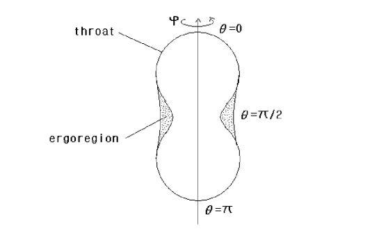
Figure 1: Plot of the cross-sectional schematic of the rotating wormhole throatT98

II Rotating wormhole

The spacetime in which we are interested will be stationary and axially symmetric. The most general stationary and axisymmetric metric can be written as

$$ds^{2}=g_{tt}dt^{2}+2g_{t\phi}dtd\phi+g_{\phi\phi}d\phi^{2}+g_{ij}dx^{i}dx^{j},$$ (1)

where the indices $i,j=1,2$. TeoT98 used the freedom to cast the metric into spherical polar coordinates by setting $g_{22}=g_{\phi\phi}/\sin^{2}x^{2}$T71 and found the metric of the rotating wormhole as:

$$ds^{2} = -N^{2}dt^{2}+e^{\mu}dr^{2}+r^{2}K^{2}d\theta^{2}+r^{2}K^{2}\sin^{2}\theta[d\phi^{2}-\Omega dt]^{2}$$

$$= -N^{2}dt^{2}+\frac{dr^{2}}{1-b(r)/r}+r^{2}K^{2}d\theta^{2}+r^{2}K^{2}\sin^{2}\theta[d\phi^{2}-\Omega dt]^{2},\$$

where $\Omega$ is the angular velocity $d\phi/dt$ acquired by a particle that falls freely from infinity to the point $(r,\theta)$, and which gives rise to the well-known dragging of inertial frames or Lense-Thirring effect in general relativity. In general, $N,b,K,\omega$ are functions of both $r$ and $\theta$. $K(r,\theta)$ is a positive, nondecreasing function that detemines the “proper radial distance” $R$ measured at $(r,\theta)$ from the origin.

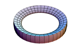
Figure 2: Ergoregion for the dumbbell-like throat wormhole model. It forms a tube.

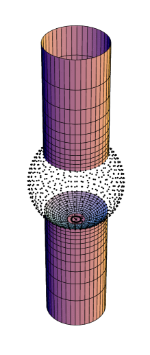
Figure 3: Ergoregion of the rigid rotating wormhole model with constant angular velocity. The dotted region is the wormhole throat.

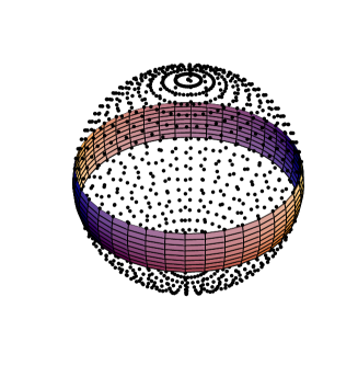
Figure 4: Ergoregion of the rigid rotating wormhole model with $\Omega=2a/r^{3}$. The dotted region is the wormhole throat. The ergoregion also forms a tube.

It is regular on the symmetry axis $\theta=0,\pi$ and two identical, asymptotically flat regions joined together at throat $r=b$. There are no event horizons or curvature singularities. The off-diagonal component of the stress-energy tensor is $T_{t\phi}$ that is interpreted as the rotation of the matter distribution.

It clearly reduces to the MT metric in the limit of zero rotation and spherical symmetry:

$$N(r,\theta)\rightarrow e^{\Lambda(r)},\quad b(r,\theta)\rightarrow b(r),\quad K(r,\theta)\rightarrow 1,\quad\omega(r,\theta)\rightarrow 0.$$ (3)

We also require that the metric should be asymptotically flat, in which case

$$N\rightarrow 1,\quad\frac{b}{r}\rightarrow 0,\quad K\rightarrow 1,\quad\omega\rightarrow 0$$ (4)

as $r\rightarrow\infty.$ Thus, $r$ is asymptotically the proper radial distance. In particular, if

$$\Omega=\frac{2a}{r^{3}}+O\left(\frac{1}{r^{4}}\right),$$ (5)

then by changing to Cartesian coordinates, it can be checked that $a$ is the total angular momentum of the wormhole.

Afterwards, the source of the rotating wormhole was considered by Bergliaffa and HibberdBH00b . They found the constraints on the Einstein tensor that arise from the matter used as a source of Einstein’s equation for a generally axially symmetric and stationary spacetime. The constraints are

$$G_{11}-G_{22}=0,\quad G_{12}=0,\quad G_{03}^{2}=(G_{00}+G_{22})(G_{11}-G_{33})$$ (6)

and

$$G_{00}+G_{33}\geq 2G_{03},\quad\left(\frac{u_{0}}{u_{3}}\right)^{2}>1,$$ (7)

where $u_{\mu}$ is the four-velocity of the fluid model of the stress-energy tensor.

III Examples of rotating wormhole

As the first example, TeoT98 took the gravitational potential of rotating wormhole metric to be

$$N=K=1+\frac{(4a\cos\theta)^{2}}{r},\quad b=1,\quad\omega=\frac{2a}{r^{3}}.$$ (8)

Note that $a$ is the angular momentum of the resulting wormhole. Proper radius $R=1+(4a\cos\theta)^{2}$ is at throat $r=1$ and the proper distance is

$$l=\pm[\sqrt{r(r-1)}+\ln(\sqrt{r}+\sqrt{r-1})].$$ (9)

If the rotation of the wormhole is sufficiently fast, $g_{tt}$ becomes positive in some region outside the throat, indicating the presence of an ergoregions where particles can no longer remain stationary with respect to infinity. This occurs when $r^{2}=|2a\sin\theta|>1$ when $|a|>1/2$. The ergoregions does not completely surround the throat, but forms a “tube” around the equatorial region instead of ergosphere in Kerr metric. The plot is in Figs. 1 and 2 which shows the cross-section of the throat and the ergoregion.

As the second example, we just think about the rigid rotating wormhole, i.e.,

$$N=K=1,\quad b=\frac{b_{0}^{2}}{r},\quad\Omega=\mbox{const.}$$ (10)

such that the metric should be

$$ds^{2}=-dt^{2}+\frac{dr^{2}}{1-\frac{b(r)}{r}}+r^{2}d\theta^{2}+r^{2}\sin^{2}\theta[d\phi-\Omega dt]^{2}.$$ (11)

Without the angular velocity, the spacetime is just the simplest wormhole model used in former papersK00 ; KL01 ; KK98 . Here, the throat is $r=b_{0}$ and the shape of the throat is a sphere. In this case, the ergoregion is when $r=1/|\Omega\sin\theta|$. When $b_{0}\Omega>1$, the ergoregion is cut by throat as in Fig. 3, while the cylinder shape ergoregion cover the whole wormhole throat, when $b_{0}\Omega\leq 1$.

When the angular velocity is the same as first example, i.e., $\Omega=2a/r^{3}$ and when $r>b_{0}$, the ergoregion is tube type for large angular momentum as shown in Fig. 4. It is similar to Fig. 2.

IV Perturbation of the wormhole

IV.1 Scalar perturbation of non-rotating wormhole

The spacetime metric for static uncharged wormhole is given as

$$ds^{2}=-e^{2\Lambda(r)}dt^{2}+\frac{dr^{2}}{1-b(r)/r}+r^{2}(d\theta^{2}+\sin^{2}\theta d\phi^{2}),$$ (12)

where $\Lambda(r)$ is the lapse function and $b(r)$ is the wormhole shape function. They are assumed to be dependent on $r$ only for static case.

The wave equation of the minimally coupled massless scalar field is given by

$$\nabla^{\mu}\nabla_{\mu}\Phi=\frac{1}{\sqrt{-g}}\partial_{\mu}(\sqrt{-g}g^{\mu\nu}\partial_{\nu}\Phi)=0.$$ (13)

In spherically symmetric space-time, the scalar field can be separated by variables,

$$\Phi_{lm}=Y_{lm}(\theta,\phi)\frac{u_{l}(r,t)}{r},$$ (14)

where $Y_{lm}(\theta,\phi)$ is the spherical harmonics and $l$ is the quantum angular momentum.

If the time dependence of the wave is harmonic as $u_{l}(r,t)=\hat{u}_{l}(r,\omega)e^{-i\omega t}$, the equation becomes

$$\left(\frac{d^{2}}{dr^{2}_{*}}+\omega^{2}-V_{l}(r)\right)\hat{u}_{l}(r,\omega)=0,$$ (15)

where the potential is

$$V_{l}(r) = \frac{L^{2}}{r^{2}}e^{2\Lambda}+\frac{1}{r}e^{\Lambda}\sqrt{1-\frac{b}{r}}\frac{\partial}{\partial r}\left(e^{\Lambda}\sqrt{1-\frac{b}{r}}\right)$$

$$= e^{2\Lambda}\left[\frac{l(l+1)}{r^{2}}-\frac{b^{\prime}r-b}{2r^{3}}+\frac{1}{r}\left(1-\frac{b}{r}\right)\Lambda^{\prime}\right]$$

and the proper distance $r_{*}$ has the following relation to $r$:

$$\frac{\partial}{\partial r_{*}}=e^{\Lambda}r^{2}\sqrt{1-\frac{b}{r}}\frac{\partial}{\partial r}.$$ (17)

Here, $L^{2}=l(l+1)$ is the square of the angular momentum. It is just the Schrödinger equation with energy $\omega^{2}$ and potential $V_{l}(r)$. When $e^{2\Lambda}$ is finite, $V_{l}$ approaches zero as $r\rightarrow\infty$, which means that the solution has the form of the plane wave $\hat{u}_{l}\sim e^{\pm i\omega r_{*}}$ asymptotically.

As the simplest example for this problem, we consider the special case $(\Lambda=0,b=b_{0}^{2}/r)$ as usual, the potential should be

$$V_{l}=\frac{l(l+1)}{r^{2}}+\frac{b_{0}^{2}}{r^{4}},$$ (18)

where the proper distance $r_{*}$ is given by

$$r_{*}=\int\frac{1}{\sqrt{1-b_{0}^{2}/r^{2}}}dr=\sqrt{r^{2}-b_{0}^{2}}.$$ (19)

IV.2 Scalar perturbation of rotating wormhole

For the rotating case, we also only think the scalar field case in this paper. By using $\sqrt{-g}=r^{2}K^{2}NL\sin\theta$, where $L^{2}=1/(1-b/r)$, the scalar wave equation becomes

$$\nabla_{\mu}\nabla^{\mu}\Phi=\frac{1}{\sqrt{-g}}\partial_{\mu}(g^{\mu\nu}\sqrt{-g}\partial_{\nu}\Phi)=0.$$ (20)

In this case we try to separate variables with $\Phi=R(r)\Theta(\theta)e^{im\phi}e^{i\omega t}$. Then the wave equation in spacetime of metric eq. (II) becomes

$$\frac{\omega^{2}}{N^{2}}+\frac{2\Omega}{N^{2}}\omega m-m^{2}\left(\frac{1}{r^{2}K^{2}\sin^{2}\theta}-\frac{\Omega^{2}}{N^{2}}\right)+\frac{1}{r^{2}K^{2}NL}\frac{1}{R}\frac{d}{dr}\left(\frac{r^{2}K^{2}N}{L}\frac{d}{dr}\right)R+\frac{1}{r^{2}K^{2}NL\sin\theta}\frac{1}{\Theta}\frac{d}{d\theta}\left(NL\sin\theta\frac{d}{d\theta}\right)\Theta=0.$$ (21)

It is very hard to separate variables, when $N,K,L$, and $\Omega$ are function of $r$ and $\theta$.

To make the problem simple, we adapt the toy model as $N=K=1,b(r)=\frac{b_{0}^{2}}{r}$, and $\Omega(r)$ such that the metric of the model spacetime is eq. (11)

$$ds^{2}=-dt^{2}+\frac{dr^{2}}{1-\frac{b(r)}{r}}+r^{2}d\theta^{2}+r^{2}\sin\theta[d\phi^{2}-\Omega(r)dt]^{2}$$ (22)

This is the just the rigid rotation of the simplest model when $\Omega$ is constant. This model means that the wormhole does not change its shape under rotation with angular velocity $\Omega$. In both cases of constant $\Omega$ and $r$-dependent $\Omega(r)$, the wave equation can be simply separated as

$$\frac{1}{\sin\theta}\frac{d}{d\theta}\left(\sin\theta\frac{d}{d\theta}\right)\Theta-\left(\frac{m^{2}}{\sin^{2}\theta}-\lambda_{lm}\right)\Theta=0$$ (23)

and

$$\frac{d^{2}u}{dr^{2}_{*}}+V_{l}(\omega,m,r,\Omega)u=0,$$ (24)

where $R(r)=\frac{u(r)}{r}.$ The proper distance $r_{*}$ is defined as

$$\frac{d}{dr_{*}}=\sqrt{1-\frac{b(r)}{r}}\frac{d}{dr}$$ (25)

which is the same as the ron-rotating caseK00 . The potential is

$$V_{l}=(\omega+\Omega m)^{2}-\frac{\lambda_{lm}}{r^{2}}-\frac{2b_{0}^{2}}{r^{4}}.$$ (26)

The separation constant $\lambda_{lm}$ becomes $l(l+1)$ in the limit of $\omega=0$. The solution to $\Theta(\theta)=S_{ml}(\theta,0)$ that is a spheroidal wave function in this case becomes the spherical harmonics when $\omega\Omega=0$.

When $r\rightarrow\infty$ in constant $\Omega$ case, the equation becomes

$$\frac{d^{2}u}{dr_{*}^{2}}+(\omega+\Omega m)^{2}u\simeq 0$$ (27)

which means

$$u\sim e^{\pm i(\omega+\Omega m)r_{*}}.$$ (28)

When $\Omega=\frac{2a}{r^{3}}$, the equation in the limit of large $r$ becomes

$$\frac{d^{2}u}{dr_{*}^{2}}+\omega^{2}u\simeq 0$$ (29)

and the solutions are

$$u\sim e^{\pm i\omega r_{*}}.$$ (30)

They are same asymptotic solutions as those of non-rotating wormhole.

V Discussion

We examined the rotating wormhole and found the Schrödinger type equation for scalar perturbation in special model of rotating wormhole. The result will be useful for considering the gravitational wave problem by the wormhole and exotic matter. Later, we will extend the problem into the gravitational perturbation like the non-rotating caseK04 to see the more realistic situations.

References

• (1) M. S. Morris and K. S. Thorne, Am. J. Phys. 56, 395 (1988).
• (2) Sung-Won Kim, Gravitation & Cosmology, 6, 337 (2000).
• (3) Sung-Won Kim and Hyunjoo Lee, Phys. Rev. D 63, 063014 (2001).
• (4) E. Teo, Phys. Rev. D 58, 024014 (1998).
• (5) S. Kar, D. Sahdev, and B. Bhawal, Phy. Rev. D 49, 853 (1994).
• (6) S. Kar, S. N. Minwalla, D. Mishra, and D. Sahdev, Phy. Rev. D 51, 1632 (1995).
• (7) S. E. P. Bergliaffa and K. E. Hibberd, Phy. Rev. D 62, 044045 (2000).
• (8) Sung-Won Kim, gr-qc/0401007.
• (9) T. Regge and J. A. Wheeler, Phys. Rev., 108, 1063 (1957).
• (10) K. S. Thorne, in General Relativity and Cosmology, edited by R. K. Sachs (Academic, New York, 1971).
• (11) S. E. P. Bergliaffa and K. E. Hibberd, gr-qc/0006041.
• (12) Sung-Won Kim and S. P. Kim, Phys. Rev. D 58, 087703 (1998).