Gravitational perturbation of traversable wormhole

Abstract

In this paper, we study the perturbation problem of the scalar, electromagnetic, and gravitational waves under the traversable Lorentzian wormhole geometry. The unified form of the potential for the Schrödinger type one-dimensional wave equation is found.

I Introduction

The wormhole has the structure which is given by two asymptotically flat regions and a bridge connecting two regionsMT88 . For the Lorentzian wormhole to be traversable, it requires exotic matter which violates the known energy conditions. To find the reasonable models, there had been studying on the generalized models of the wormhole with other matters and/or in various geometries. Among the models, the matter or wave in the wormhole geometry and its effect such as radiation are very interesting to us. The scalar field could be considered in the wormhole geometry as the primary and auxiliary effectsK00 . Recently, the solution for the electrically charged case was also found KL01 .

Scalar wave solutions in the wormhole geometryKSB94 ; KMMS95 was in special wormhole model only and the transmission and reflection coefficients were found. The electromagnetic wave in wormhole geometry is recently discussedBH00 along the method of scalar field case. These wave equations in wormhole geometry draws attention to the research on radiation and wave.

Also there was a suggestion that the wormhole would be one of the candidates of the gamma ray burstsTRA98 . With such suggestions, we can also suggest the wormhole as one of the candidates of the gravitational wave sources. If the gravitational wave detections are achieved in future, the identification of the wormhole might be followed by the unique waveforms from the perturbed exotic matter consisting of wormhole.

For the gravitational radiation in any forms, the scattering problem to calculate the cross section in more generalized models of wormhole should be considered. Thus the study of scalar, electromagnetic, and gravitational waves under wormhole geometry is necessary to the research on the gravitational radiation.

In this paper, we found the general form of the gravitational perturbation of the traversable wormhole, which will be a key to extend the wormhole physics into the problems similar to those relating to gravitational wave of black holes. The main idea and resultant equation is similar to Regge-Wheeler equationRW57 for black hole perturbation. Here we adopt the geometrical unit, i.e., $G=c=\hbar=1$.

II Scalar perturbation

The spacetime metric for static uncharged wormhole is given as

$$ds^{2}=-e^{2\Lambda(r)}dt^{2}+\frac{dr^{2}}{1-b(r)/r}+r^{2}(d\theta^{2}+\sin^{2}\theta d\phi^{2}),$$ (1)

where $\Lambda(r)$ is the lapse function and $b(r)$ is the wormhole shape function. They are assumed to be dependent on $r$ only for static case.

The wave equation of the minimally coupled massless scalar field is given by

$$\nabla^{\mu}\nabla_{\mu}\Phi=\frac{1}{\sqrt{-g}}\partial_{\mu}(\sqrt{-g}g^{\mu\nu}\partial_{\nu}\Phi)=0.$$ (2)

In spherically symmetric space-time, the scalar field can be separated by variables,

$$\Phi_{lm}=Y_{lm}(\theta,\phi)\frac{u_{l}(r,t)}{r},$$ (3)

where $Y_{lm}(\theta,\phi)$ is the spherical harmonics and $l$ is the quantum angular momentum.

If $l=0$ and the scalar field $\Phi(r)$ depends on $r$ only, the wave equation simply becomes the following relationKK98 :

$$e^{\Lambda}\sqrt{1-\frac{b}{r}}r^{2}\frac{\partial}{\partial r}\Phi=A=\mbox{const.}$$ (4)

In this relation, the back reaction of the scalar wave on the wormhole geometry is neglected. Thus the static scalar wave without propagation is easily found as the integral form of

$$\Phi=A\int e^{-\Lambda}r^{-2}\left(1-\frac{b}{r}\right)^{-1/2}dr.$$ (5)

The scalar wave solution was already given to us for the special case of wormhole in Ref. KL01 ; KK98 .

More generally, if the scalar field $\Phi$ depends on $r$ and $t$, the wave equation after the separation of variables $(\theta,\phi)$ becomes

$$-\ddot{u}_{l}+\frac{\partial^{2}u_{l}}{\partial r_{*}^{2}}=V_{l}\,\,u_{l},$$ (6)

where the potential is

$$V_{l}(r) = \frac{L^{2}}{r^{2}}e^{2\Lambda}+\frac{1}{r}e^{\Lambda}\sqrt{1-\frac{b}{r}}\frac{\partial}{\partial r}\left(e^{\Lambda}\sqrt{1-\frac{b}{r}}\right)$$

$$= e^{2\Lambda}\left[\frac{l(l+1)}{r^{2}}-\frac{b^{\prime}r-b}{2r^{3}}+\frac{1}{r}\left(1-\frac{b}{r}\right)\Lambda^{\prime}\right]$$

and the proper distance $r_{*}$ has the following relation to $r$:

$$\frac{\partial}{\partial r_{*}}=e^{\Lambda}r^{2}\sqrt{1-\frac{b}{r}}\frac{\partial}{\partial r}.$$ (8)

Here, $L^{2}=l(l+1)$ is the square of the angular momentum.

The properties of the potential are determined by the shape of it, if only the explicit forms of $\Lambda$ and $b$ are given. If the time dependence of the wave is harmonic as $u_{l}(r,t)=\hat{u}_{l}(r,\omega)e^{-i\omega t}$, the equation becomes

$$\left(\frac{d^{2}}{dr^{2}_{*}}+\omega^{2}-V_{l}(r)\right)\hat{u}_{l}(r,\omega)=0.$$ (9)

It is just the Schrödinger equation with energy $\omega^{2}$ and potential $V_{l}(r)$. When $e^{2\Lambda}$ is finite, $V_{l}$ approaches zero as $r\rightarrow\infty$, which means that the solution has the form of the plane wave $\hat{u}_{l}\sim e^{\pm i\omega r_{*}}$ asymptotically. The result shows that if a scalar wave passes through the wormhole the solution is changed from $e^{\pm i\omega r}$ into $e^{\pm i\omega r_{*}}$, which means that the potential affects the wave and experience the scattering.

As the simplest example for this problem, we consider the special case $(\Lambda=0,b=b_{0}^{2}/r)$ as usual, the potential should be in terms of $r$ or $r_{*}$ as

$$V_{l}=\frac{l(l+1)}{r^{2}}+\frac{b_{0}^{2}}{r^{4}}~{}\stackrel{{\scriptstyle\mbox{or}}}{{=}}~{}\frac{l(l+1)}{r_{*}^{2}+b_{0}^{2}}+\frac{b_{0}^{2}}{(r_{*}^{2}+b_{0}^{2})^{2}},$$ (10)

where the proper distance $r_{*}$ is given by

$$r_{*}=\int\frac{1}{\sqrt{1-b_{0}^{2}/r^{2}}}dr=\sqrt{r^{2}-b_{0}^{2}}.$$ (11)

There is the hyperbolic relation between $r_{*}$ and $r$ which is plotted in Fig. 1. The potentials are depicted in Fig. 2. The potential has the maximum value as

$$V_{l}(r_{*})|_{\rm max}=V_{l}(0)=\frac{l(l+1)+1}{b_{0}^{2}}.$$ (12)

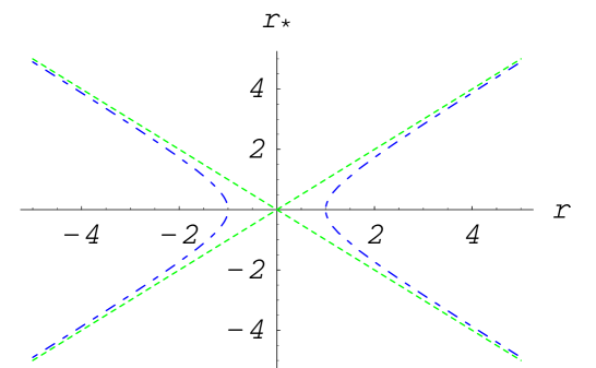
Figure 1: Plot of the proper distance $r_{*}$ versus $r$. Here we set $b_{0}=1$. The dotted line is the asymptotic line to the hyperbolic relation, the dashed line.

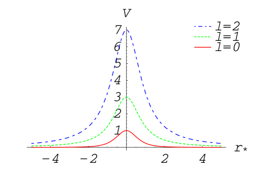
Figure 2: Plot of the potentials of the scalar wave under the specified wormhole $b=b_{0}^{2}/r$ in terms of $r_{*}$ for $l=1,2,3$. Here we set $b_{0}=1$. To have a positive potential, $l\geq 0$.

III Electromagnetic Wave

We just followed the result of Bergliaffa and HibberdBH00 . They used the electromagnetic wave under wormhole geometry of the Morris-Thorne type wormhole like our model. Maxwell’s equation in a gravitational field is

$${H^{\mu\nu}}_{;\nu}=4\pi I^{\mu},\quad H_{\mu\nu,\sigma}+H_{\nu\sigma,\mu}+H_{\sigma\mu,\nu}=0,$$ (13)

where

$$H^{\mu\nu}\equiv\sqrt{-g}F^{\mu\nu},\quad I^{\mu}\equiv\sqrt{-g}J^{\mu}$$ (14)

and the electromagnetic field strength tensors are defined by

$$F_{\mu\nu}\rightarrow(\vec{E},\vec{B}),\quad H^{\mu\nu}\rightarrow(-\vec{D},\vec{H}).$$ (15)

Defining the vectors

$$\vec{F}^{\pm}\equiv\vec{E}\pm i\vec{H},\quad\vec{S}^{\pm}\equiv\vec{D}\pm i\vec{B},$$ (16)

the Einstein-Maxwell equations are

$$\vec{\nabla}\wedge\vec{F}^{\pm}=\pm i\frac{\partial\vec{S}^{\pm}}{\partial t}=\pm in\frac{\partial\vec{F}^{\pm}}{\partial t},$$ (17)

$$\vec{\nabla}\cdot\vec{S}^{\pm}=0,$$ (18)

where $n$ is the refraction index

$$\varepsilon_{ik}=\mu_{ik}=-\sqrt{-g}\frac{g_{ik}}{g_{00}}\equiv n\delta_{ik}$$ (19)

for a medium characterized by diagonal electric and magnetic permeabilities.

The Morris-Thorne type wormhole metric, Eq. (1) can be rewritten as

$$ds^{2} = -e^{2\Lambda(r)}dt^{2}+\left(1-\frac{b(r)}{r}\right)^{-1}dr^{2}+r^{2}d\Omega^{2}$$ (20)

$$= -e^{2\Lambda(r)}dt^{2}+A^{2}(\rho)(d\rho^{2}+\rho^{2}d\Omega^{2}),$$

where $A(\rho)$ is defined by

$$n(\rho)=\frac{A(\rho)}{e^{\Lambda(\rho)}}$$ (21)

Here we consider the the special case ($\Lambda(\rho)=0,b(r)=\frac{b_{0}^{2}}{r}$) like the scalar wave case. The Herz vector is decomposed into

$$\vec{F}^{\pm}(\rho,t)=\sum_{J,M}\vec{F}^{\pm}_{JM}(\rho,t)$$ (22)

with the generalized spherical harmonics $\vec{Y}^{(\lambda)}_{JM}(\hat{\rho})$

$$\vec{F}^{\pm}_{JM}(\rho,t)=\sum_{\lambda=e,m,o}F^{\pm}_{JM}(\rho,\omega)\vec{Y}^{(\lambda)}_{JM}(\hat{\rho})e^{-i\omega t}.$$ (23)

The Maxwell equation becomes

$$-\frac{d}{d\rho}(\rho F^{\pm(m)}_{JM})=\pm n\omega\rho F^{\pm(e)}_{JM},$$ (24)

$$\frac{d}{d\rho}(\rho F^{\pm(e)}_{JM})-\sqrt{J(J+1)}F^{\pm(o)}_{JM}=\pm n\omega F^{\pm(m)}_{JM},$$ (25)

and

$$-\frac{1}{\rho}\sqrt{J(J+1)}F^{\pm(m)}_{JM}=\pm n\omega F^{\pm(o)}_{JM}.$$ (26)

Let the new coordinate $x$ be

$$\frac{dx}{d\rho}=n(\rho),\quad x=\pm\sqrt{r^{2}-b_{0}^{2}}$$ (27)

and introduce the function

$$\chi^{\pm(\lambda)}_{JM}(x,\omega)=\rho(x)F^{\pm(\lambda)}_{JM}[\rho(x),\omega].$$ (28)

Here $x$ plays the role of the proper distance $r_{*}$. The wave equation is finally

$$\frac{d^{2}\chi^{\pm(m)}_{JM}}{dz^{2}}+[\omega^{2}b_{0}^{2}-U_{J}(z)]\chi^{\pm(m)}_{JM}=0,$$ (29)

where $z=x/b_{0}$ and the potential is

$$U_{J}(z)=4J(J+1)\left[\frac{z+\sqrt{1+z^{2}}}{(z+\sqrt{1+z^{2}})^{2}+1}\right]^{2}.$$ (30)

The potential in our context becomes

$$V(r)=\frac{l(l+1)}{r^{2}}$$ (31)

The potentials are depicted in Fig. 3. Here $l\geq 1$ for the positive potential.

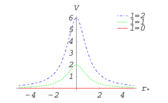
Figure 3: Plot of the potentials of the electromagnetic wave under the specified wormhole $b=b_{0}^{2}/r$ for $l=1,2,3$. Here we set $b_{0}=1$. To have a positive potential, $l\geq 1$.

IV Gravitational Perturbation

We follow the conventions of Chandrasekhar in Ref. C83 where the gravitational perturbations are derived. Start from the axially symmetric spacetime which is given by

$$ds^{2}=-e^{2\nu}dt^{2}+e^{2\psi}(d\phi-q_{1}dt-q_{2}dr-q_{3}d\theta)^{2}+e^{2\mu_{2}}dr^{2}+e^{2\mu_{3}}d\theta^{2}.$$ (32)

For unperturbed case, the wormhole spacetime is

$$e^{2\nu}=e^{2\Lambda},\quad e^{-2\mu_{2}}=\left(1-\frac{b}{r}\right)=\frac{\Delta}{r^{2}},\quad\Delta=r^{2}-br,\quad e^{\mu_{3}}=r,\quad e^{\psi}=r\sin\theta$$ (33)

and

$$q_{1}=q_{2}=q_{3}=0.$$ (34)

Axial perturbations are characterized by the nonvanishing of small $q_{1}$, $q_{2}$, and $q_{3}$. When there are linear perturbations $\delta\nu,\delta\psi,\delta\mu_{2},\delta\mu_{3}$, then there are polar perturbations with even parity which will not be considered here. From Einstein’s equation

$$(e^{3\psi+\nu-\mu_{2}-\mu_{3}}Q_{23})_{,3}=-e^{3\psi-\nu-\mu_{2}+\mu_{3}}Q_{02,0}$$ (35)

where $x^{2}=r,x^{3}=\theta$ and $Q_{AB}=q_{A,B}-q_{B,A},Q_{A0}=q_{A,0}-q_{1,A}.$ This becomes

$$\frac{e^{\Lambda}}{\sqrt{\Delta}}\frac{1}{r^{3}\sin^{3}\theta}\frac{\partial Q}{\partial\theta}=-(q_{1,2}-q_{2,0})_{,0}$$ (36)

where $Q$ is

$$Q(t,r,\theta)=\Delta Q_{23}\sin^{3}\theta=\Delta(q_{2,3}-q_{3,2})\sin^{3}\theta.$$ (37)

Another equation

$$(e^{3\psi+\nu-\mu_{2}-\mu_{3}}Q_{23})_{,2}=e^{3\psi-\nu+\mu_{2}-\mu_{3}}Q_{03,0}$$ (38)

This becomes

$$\frac{e^{\Lambda}\sqrt{\Delta}}{r^{3}\sin^{3}\theta}\frac{\partial Q}{\partial\theta}=(q_{1,3}-q_{3,0})_{,0}$$ (39)

If the time dependence is $e^{i\omega t}$, then

$$\frac{e^{\Lambda}}{\sqrt{\Delta}}\frac{1}{r^{3}\sin^{3}\theta}\frac{\partial Q}{\partial\theta} = -i\omega q_{1,2}-\omega^{2}q_{2}$$ (40)

$$\frac{e^{\Lambda}\sqrt{\Delta}}{r^{3}\sin^{3}\theta}\frac{\partial Q}{\partial\theta} = +i\omega q_{1,3}+\omega^{2}q_{3}.$$ (41)

Let $Q(r,\theta)=Q(r)C^{-3/2}_{l+2}(\theta)$, where Gegenbauer function $C^{\nu}_{n}(\theta)$ satisfy the differential equation

$$\left[\frac{d}{d\theta}\sin^{2\nu}\theta\frac{d}{d\theta}+n(n+2\nu)\sin^{2\nu}\theta\right]C^{\nu}_{n}(\theta)=0.$$ (42)

Then

$$re^{\Lambda}\sqrt{\Delta}\frac{d}{dr}\left(\frac{e^{\Lambda}\sqrt{\Delta}}{r^{3}}\frac{dQ}{dr}\right)-\mu^{2}\frac{e^{2\Lambda}}{r^{2}}Q+\omega^{2}Q=0,$$ (43)

where $\mu^{2}=(l-1)(l+2)$. If $Q=rZ$ and $\frac{d}{dr_{*}}=e^{\Lambda}\sqrt{\Delta}\frac{1}{r}\frac{d}{dr}$,

$$\left(\frac{d^{2}}{dr_{*}^{2}}+\omega^{2}-V(r)\right)Z=0,$$ (44)

where the potential is

$$V(r)=e^{2\Lambda}\frac{1}{r^{3}}\left[\mu^{2}r+\frac{3\Delta}{r}-\Delta\Lambda^{\prime}-\frac{1}{2}\Delta^{\prime}\right]$$ (45)

or

$$V(r)=e^{2\Lambda}\left[\frac{l(l+1)}{r^{2}}+\frac{b^{\prime}r-5b}{2r^{3}}-\frac{1}{r}\left(1-\frac{b}{r}\right)\Lambda^{\prime}\right]$$ (46)

in terms of $b$ and $\Lambda$. The first term is the same as the former two cases, but the signs and coefficients of the second and third terms are different from the scalar and electromagnetic wave cases.

For the simplest special case ($\Lambda=0,b=b_{0}^{2}/r$) like the former cases, the potential is

$$V(r)=\frac{l(l+1)}{r^{2}}-\frac{3b_{0}^{2}}{r^{4}},$$ (47)

whose shapes are shown in Fig. 4. By comparing with scalar and electromagnetic cases, the unified general formula is

$$V(r)=\frac{l(l+1)}{r^{2}}+\frac{(1-s^{2})b_{0}^{2}}{r^{4}},$$ (48)

where $s=0,1,2$ is spin, or

$$V(r)=\frac{l(l+1)}{r^{2}}+\frac{\lambda b_{0}^{2}}{r^{4}},$$ (49)

where $\lambda=(1-s^{2})=1,0,-3$ for scalar, electromagnetic, and gravitational perturbations, respectively. This unified form is similar to the black hole case. The condition of the positive potential is $l\geq s$.

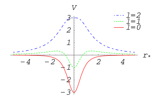
Figure 4: Plot of the potentials of the gravitational wave under the specified wormhole $b=b_{0}^{2}/r$ for $l=1,2,3$. Here we set $b_{0}=1$. To have a positive potential, $l\geq 2$.

V Discussion

We found the Regge-Wheeler type equation for gravitational perturbation. This unified form will give us new ideas and insights in the areas of wormhole physics and gravitational wave. In this paper we only consider the axially perturbation for simplicity. For further problems, ZerilliZ70 type equation should be considered in order to see the exotic matter perturbation, and checked whether the potential form is similar to that of our Regge-Wheeler type potential like the black hole case or not.

References

(1) M. S. Morris and K. S. Thorne, Am. J. Phys. 56, 395 (1988).
(2) S.-W. Kim, Gravitation & Cosmology, 6, 337 (2000).
(3) S.-W. Kim and H. Lee, Phys. Rev. D 63, 063014 (2001).
(4) S. Kar, D. Sahdev, and B. Bhawal, Phy. Rev. D
49, 853 (1994).
(5) S. Kar, S. N. Minwalla, D. Mishra, and D. Sahdev,
Phy. Rev. D 51, 1632 (1995).
(6) S. E. P. Bergliaffa and K. E. Hibberd, Phy. Rev. D 62, 044045
(2000).
(7) D. Torres, G. Romero, and L. Anchordoqui, Phy. Rev. D 58,
123001 (1998).
(8) T. Regge and J. A. Wheeler, Phys. Rev., 108,
1063 (1957).
(9) S.-W. Kim and S. P. Kim, Phys. Rev. D 58, 087703 (1998).
(10) S. Chandrasekhar, Mathematical Theory of Black Holes (Clarendon Press, Oxford, 1988).