For scalar, electromagnetic, or gravitational wave propagation on a background Schwarzschild blackhole, we describe the exact nonlocal radiation outer boundary conditions (robc) appropriate for a spherical outer boundary of finite radius enclosing the blackhole. Derivation of the robc is based on Laplace and spherical–harmonic transformation of the Regge–Wheeler equation, the pde governing the wave propagation, with the resulting radial ode an incarnation of the confluent Heun equation. For a given angular integer $l$ the robc feature integral convolution between a time–domain radiation boundary kernel (tdrk) and each of the corresponding $2l+1$ spherical–harmonic modes of the radiating wave field. The tdrk is the inverse Laplace transform of a frequency–domain radiation kernel (fdrk) which is essentially the logarithmic derivative of the asymptotically outgoing solution to the radial ode. We numerically implement the robc via a rapid algorithm involving approximation of the fdrk by a rational function. Such an approximation is tailored to have relative error $\varepsilon$ uniformly along the axis of imaginary Laplace frequency. Theoretically, $\varepsilon$ is also a long–time bound on the relative convolution error. Via study of one–dimensional radial evolutions, we demonstrate that the robc capture the phenomena of quasinormal ringing and decay tails. Moreover, carrying out a numerical experiment in which a wave packet strikes the boundary at an angle, we find that the robc yield accurate results in a three–dimensional setting. Our work is a partial generalization to Schwarzschild wave propagation and Heun functions of the methods developed for flatspace wave propagation and Bessel functions by Alpert, Greengard, and Hagstrom (agh), save for one key difference. Whereas agh had the usual armamentarium of analytical results (asymptotics, order recursion relations, bispectrality) for Bessel functions at their disposal, what we need to know about Heun functions must be gathered numerically as relatively less is known about them. Therefore, unlike agh, we are unable to offer an asymptotic analysis of our rapid implementation.                                            
^† Based on Reference [1]. Published as two separate articles in J. Comp. Phys. 199, issue 1, 376-422 (2004) and Class. and Quantum Grav. 21, 4147-4192 (2004).
^‡ Now at Center for Gravitational Wave Astronomy, University of Texas at Brownsville, 80 Fort Brown, Brownsville TX, 78520. Email address: lau@phys.utb.edu.

List of main symbols

Section 1.1.1, $\mathrm{d}s^{2}$notation for generic line–element
$T$static time coordinate
$r$areal radius coordinate
$\theta,\phi$standard angular coordinates
$\mathrm{m}$geometrical mass of blackhole
$g_{\alpha\beta}$metric tensor
$\tau$dimensionless static time $T/(2\mathrm{m})$
$\rho$dimensionless radius $r/(2\mathrm{m})$
$F$ubiquitous metrical function $1-1/\rho=1-2\mathrm{m}/r$
$\rho_{*}$tortoise coordinate $\rho+\log(\rho-1)$
$\mu$dimensionless retarded time $\tau-\rho_{*}$
$\nu$dimensionless advanced time $\tau+\rho_{*}$
  (also used as Bessel order below)
Section 1.1.2, $\square$d’Alembertian or wave operator
$\psi$wave field in coordinates $(\tau,\rho,\theta,\phi)$ or $(T,r,\theta,\phi)$
$x^{\alpha}$generic coordinate function
$\sqrt{-g}$square root of (minus) determinant of metric
$g^{\alpha\beta}$inverse metric tensor
$\jmath$spin, takes values 0,1,2 only
$l$primary harmonic angular index, runs from $\jmath$ to $\infty$
$m$secondary harmonic angular index, runs from $-l$ to $l$
  (this is italic $m$, not plain $\mathrm{m}$ which is the mass)
$Y_{lm}(\theta,\phi)$spherical harmonic
$\psi_{lm}(\tau,\rho)$spherical–harmonic transform of $\psi$
$\psi_{l}$$\psi_{lm}(\tau,\rho)$ with coordinates and index $m$ suppressed
$\Psi_{l}$$\rho\psi_{l}$
$V(\rho)$Regge–Wheeler potential
$\varphi_{l}$$\psi_{l}(\mu+\rho_{*},\rho)$, that is $\psi_{l}$ in retarded time coordinates
$\Phi_{l}$$\rho\varphi_{l}$, same as $\Psi_{l}(\mu+\rho_{*},\rho)$,
  that is $\Psi_{l}$ in retarded time coordinates
Section 1.2.1, $\mathcal{L}$Laplace transform operation
$\sigma$dimensionless Laplace frequency $2\mathrm{m}s$
$s$Laplace frequency
Section 1.2.2, $\hat{\psi}_{l}$Laplace transform (on $\tau$) of $\psi_{l}$
  and generic solution to radial ode
$z$the product $\sigma\rho$
$k_{l}(z)$, $i_{l}(z)$modified spherical Bessel functions
$K_{l+1/2}(z)$, $I_{l+1/2}(z)$modified cylindrical Bessel functions
Section 1.2.3, $\hat{\Psi}_{l}$Laplace transform (on $\tau$) of $\Psi_{l}$
$\rho_{B}$dimensionless outer radius
Section 1.3.1, $\Theta_{l}$generic solution to normal form of radial ode
$\hat{\varphi}_{l}$Laplace transform (on $\mu$) of $\varphi_{l}$, also $\Theta_{l}$ for $\jmath=0$ case
Section 1.3.2, $\hat{\Phi}_{l}$Laplace transform (on $\mu$) of $\Phi_{l}$ and generic
  solution to normalized form of radial ode
$W_{l}(\sigma\rho;\sigma)$ outgoing solution $\hat{\Phi}_{l}^{+}(\rho;\sigma)$ to
  normalized form of radial ode
$Z_{l}(\sigma\rho;\sigma)$ ingoing solution $\hat{\Phi}_{l}^{-}(\rho;\sigma)$ to
  normalized form of radial ode
$W_{l}(\sigma\rho)$, $Z_{l}(\sigma\rho)$corresponding Bessel–type functions
Section 1.3.3, $\kappa$$1-\jmath^{2}$, takes values $1,0,-3$ only
$d_{n}(\sigma)$coefficients in asymptotic expansion for $W_{l}(z;\sigma)$
$c_{n}$coefficients in asymptotic expansion for $W_{l}(z)$
Section 1.4.1, $\mathsf{N}$$F^{1/2}$, temporal lapse for $(\tau,\rho)$ coordinates
$\mathsf{M}$$F^{-1/2}$, radial lapse for $(\tau,\rho)$ coordinates
$*$Laplace convolution
$\mathcal{L}^{-1}$inverse Laplace transform operation
$\omega_{l}(\tau;\rho_{B})$time–domain radiation kernel (tdrk)
$\hat{\omega}_{l}(\sigma;\rho_{B})$frequency–domain radiation kernel (fdrk)
$\omega(\tau)$, $\hat{\omega}(\sigma)$same objects with $l$ and $\rho_{B}$ suppressed
Section 1.4.2, $N_{l}(\rho_{B})$number of poles for $\hat{\omega}_{l}(\sigma;\rho_{B})$
$\sigma_{l,n}(\rho_{B})$pole location for $\hat{\omega}_{l}(\sigma;\rho_{B})$
$\alpha_{l,n}(\rho_{B})$pole strength for $\hat{\omega}_{l}(\sigma;\rho_{B})$
$\chi$continuous variable on $[0,\infty)$ and coordinate for cut
$f_{l}(\chi;\rho_{B})$cut profile for $\hat{\omega}_{l}(\sigma;\rho_{B})$
$N$, $\alpha_{n}$, $\sigma_{n}$, $f(\chi)$ same variables with all $l$ and
  $\rho_{B}$ dependence suppressed
Section 1.4.3, $G_{l}(\rho_{*},\rho_{*}^{\prime},\tau)$time–domain Green’s function.
$\hat{G}_{l}(\rho_{*},\rho_{*}^{\prime},\sigma)$frequency–domain Green’s function.
Section 1.4.4, $\xi(\tau)$approximate time–domain radiation kernel
$y$$\mathrm{Im}\sigma$
$\hat{\xi}(\sigma)$approximate frequency–domain radiation kernel
$P(\sigma)$polynomial in $\sigma$ of degree $d-1$
$Q(\sigma)$polynomial in $\sigma$ of degree $d$
$\varepsilon$relative error tolerance
$\Delta\hat{\omega}(\sigma)$numerical error in $\hat{\omega}(\sigma)$
Section 2.1.1, $p$integer appearing in cutoff $l-p$
  for asymptotic expansions
Section 2.1.2, $\theta$an angle in $z$–plane
$I$, $J$, $N$, $M$integer constants
Section 2.1.3, $k_{l,n}$$n$th zero of the Bessel function $K_{l+1/2}(z)$
$\mathcal{C}$asymptotic curve on which the $k_{l,n}$ accumulate
$P$integer constant
Introduction for Section 2.2, $w_{l}(z)$$zW_{l}^{\prime}(z)/W_{l}(z)$
$w_{l}(z;\sigma)$$zW_{l}^{\prime}(z;\sigma)/W_{l}(z;\sigma)$
Section 2.2.3, $a_{n}$coefficients used in closed–form
  expression for origin value of the kernel
Section 2.2.4, $u_{l}(z;\sigma)$$\mathrm{Re}w_{l}(z;\sigma)$
$v_{l}(z;\sigma)$$\mathrm{Im}w_{l}(z;\sigma)$
$u_{l}(z)$$\mathrm{Re}w_{l}(z)$
$v_{l}(z)$$\mathrm{Im}w_{l}(z)$
Section 3.1.1, $\mathbb{S}$parameter space $\jmath=0,\rho_{B}\in[15,25],0\leq l\leq 10$
Section 3.2.1, $T_{l,n}(1/\rho_{B})$interpolating polynomial for pole locations
Section 3.3.1, $\nu$Bessel order $l+1/2$, not advanced time
$x$$\mathrm{Re}\sigma$
$d$degree of polynomial $Q(\sigma)$
Section 3.3.3, $\beta_{n}$ pole location for compressed kernel
$\gamma_{n}$pole strength for compressed kernel
Section 4.1.1, $H$horizon, inner two–surface at $r=2\mathrm{m}$
$r_{*}$physical tortoise coordinate $r+2\mathrm{m}\log(r/(2\mathrm{m})-1)$
$v$physical advanced time $2\mathrm{m}\nu=T+r_{*}$
$u$physical retarded time $2\mathrm{m}\mu=T-r_{*}$
$T_{v}$time variable $T+2\mathrm{m}\log(r/(2\mathrm{m})-1)$
  closely related to $v=T_{v}+r$
$T_{u}$time variable $T-2\mathrm{m}\log(r/(2\mathrm{m})-1)$
  closely related to $u=T_{u}-r$
$t$time variable for numerical implementation,
  $T_{v}$ shifted by suitable constant
$\Sigma$spacetime foliation determined by
  $t$ and also a generic level–$t$ slice
$N$temporal lapse for $(t,r)$ coordinates,
$M$radial lapse function for $(t,r)$ coordinates
$V^{r}$shift vector for $(t,r)$ coordinates
Section 4.1.2, $U$field $\psi_{lm}(\tau,\rho)$ from Section 1.1.2 but now in terms of
  $(t,r)$ coordinates and with $l$ and $m$ suppressed
Section 4.1.3, $e_{\bot}$normal vector for a $\Sigma$ slice
$e_{\vdash}$ normal vector for a round sphere in a $\Sigma$ slice
$e_{+}$null vector $e_{\bot}+e_{\vdash}$
$X$characteristic derivative $e_{+}[U]$,
  also with $l$ and $m$ indices suppressed
Section 4.1.4, $S(r,X,U,\partial_{r}U)$source for $X$ evolution equation
Section 4.2.1, $r_{B}$outer boundary radius $2\mathrm{m}\rho_{B}$
$Q$number of subintervals for radial mesh
$r_{q}$radial mesh point
$\Delta r$, $\Delta t$radial and temporal discretization steps
$U^{n}_{q}$, $N_{q}$, $[X_{-}^{M}]_{q}$examples of mesh functions
  $U(t_{n},r_{q})$, $N(r_{q})$, $X^{M}_{-}(r_{q})$
$\bar{U}{}^{n+1}_{q}$, $\bar{X}{}^{n+1}_{q}$predicted variables
$\widetilde{U}{}^{n+1}_{q}$, $\widetilde{X}{}^{n+1}_{q}$corrected variables
Section 4.2.2, $r_{-1}$ghost point $2\mathrm{m}-\Delta r$ inside horizon
Section 4.3.1, $\mathsf{e}_{+}$null vector $\mathsf{N}^{-1}\partial/\partial T+\mathsf{M}^{-1}\partial/\partial r$
$\vartheta$hyperbolic angle in the identity $\mathsf{e}_{+}=e^{\vartheta}e_{+}$
$\mathsf{X}_{l}$characteristic derivative $\mathsf{e}_{+}[\psi_{l}]$
$\Omega_{l}(T;r_{B})$physical time–domain radiation kernel
Section 4.3.3, $\beta_{n}^{R},\beta_{n}^{I}$real and imaginary parts of $\beta_{n}$ from Section 3.3.3
$\gamma_{n}^{R},\gamma_{n}^{I}$real and imaginary parts of $\gamma_{n}$ from Section 3.3.3
$b_{n}^{R}+\mathrm{i}b_{n}^{I}$$(\beta_{n}^{R}+\mathrm{i}\beta_{n}^{I})/(2\mathrm{m})$
$c_{n}^{R}+\mathrm{i}c_{n}^{I}$$(\gamma_{n}^{R}+\mathrm{i}\gamma_{n}^{I})/(2\mathrm{m})$
$\Xi(t)$approximate time–domain radiation kernel
$d_{\mathrm{sing}}$number of approximating poles on negative real axis
$d_{\mathrm{pair}}$number of conjugate pairs of approximating poles
$\mu_{i}$reordered pole location on negative
  real axis, not retarded time
$\kappa_{i}$ reordered pole strength on negative real axis
$m_{j}^{R}+\mathrm{i}m_{j}^{I}$reordered pole strength
$k_{j}^{R}+\mathrm{i}k_{j}^{I}$reordered pole location,
$H_{i}(t)$cut piece of the kernel $\Xi(t)$ built with $\mu_{i}$ and $\kappa_{i}$
$G_{j}(t)$ringing piece of kernel $\Xi(t)$ built
  with $m_{j}^{R}+\mathrm{i}m_{j}^{I}$ and $k_{j}^{R}+\mathrm{i}k_{j}^{I}$
$F_{j}(t)$auxiliary kernel built with $m_{j}^{R}+\mathrm{i}m_{j}^{I}$ and $k_{j}^{R}+\mathrm{i}k_{j}^{I}$
${}_{\mathtt{H}}(\Xi*U)$, ${}_{\mathtt{L}}(\Xi*U)$notation for history and local
  parts of integral convolution
Section 4.3.4, $\mathsf{N}_{B}$$\mathsf{N}(r_{B})$
${}_{\mathtt{L}}\overline{(\Xi*U)}{}^{n+1}$predicted local part of convolution
${}_{\mathtt{L}}\widetilde{(\Xi*U)}{}^{n+1}$corrected local part of convolution
Section 5.1.1, $f$one–dimensional bump function
$A$, $a$, $b$, $\delta$parameters specifying $f$
$U^{\mathrm{free}}$free solution
$U^{\mathrm{ROBC}}$robc solution
$U^{\mathrm{SOBC}}$Sommerfeld solution
Section 5.2.1, $f$three–dimensional bump function
$\mathbf{r}$, $\mathbf{v}$, $\mathbf{r}_{0}$, $v_{x}$, $v_{y}$, $v_{z}$, $x_{0}$, $y_{0}$, $z_{0}$parameters specifying $f$
$U_{lm}$, $X_{lm}$$U$ and $X$, but now with $l$ and $m$ indices
$(r_{q},\theta_{i}$, $\phi_{j})$spherical polar grid
Section 5.2.2, $\mathrm{vol}(\Sigma)$volume of spatial slice $\Sigma$

0. Introduction

0.1. Background

Consider the Cauchy problem for the scalar wave equation,

(1) $$-\partial^{2}_{t}U+\Delta U=0\,,$$

on $[t_{0},t_{F}]\times\mathbb{E}^{3}$, the Cartesian product of a closed time interval and Euclidean three–space. First, we specify suitable initial–value or canonical data $U|_{t_{\mathrm{0}}}$ and $\partial_{t}U|_{t_{0}}$ on $\mathbb{E}^{3}$ at the initial time $t_{0}$. Next, using the rule (1), we evolve the data until the final time $t_{F}$, along the way generating the solution $U$ throughout the temporally bounded but spatially unbounded domain $[t_{0},t_{F}]\times\mathbb{E}^{3}$. Provided physically reasonable initial data, this problem is well–posed; however, it is not the evolution problem one typically encounters in numerical wave simulation. Usually the numerical mesh covers only a finite portion of $\mathbb{E}^{3}$.

With the finiteness of numerical meshes in mind, consider the following more realistic evolution problem. Let $\Sigma\subset\mathbb{E}^{3}$ be a round, solid, three–dimensional ball determined by $r\leq r_{B}$, with $r_{B}$ a fixed outer radius, on which we specify compactly supported initial data $U|_{t_{0}}$ and $\partial_{t}U|_{t_{0}}$ at $t=t_{0}$. Again, the goal is to evolve the data, although now generating the solution $U$ on the finite domain $\mathcal{M}=[t_{0},t_{F}]\times\Sigma$ depicted in Fig. 1. Respectively, let $\Sigma_{0}$ and $\Sigma_{F}$ denote the ball $\Sigma$ at $t=t_{0}$ and $t=t_{F}$. One element of the boundary $\partial\mathcal{M}=\Sigma_{0}\cup\Sigma_{F}\cup{}^{3}\!B$ is a timelike three–dimensional cylinder ${}^{3}\!B$ determined by $t_{0}\leq t\leq t_{F}$ and $r=r_{B}$. Note that ${}^{3}\!B$ is the history in time of the spherical spatial boundary $B=\partial\Sigma$. As it stands, such an evolution problem is not well–posed, since $\mathcal{M}$ is larger than the future domain of dependence of $\Sigma_{0}$. Indeed, $U|_{t_{0}}$ and $\partial_{t}U|_{t_{0}}$ are free data, and we have no control over data on $\mathbb{E}^{3}/\Sigma_{0}$, the region exterior to the initial $\Sigma$ ball. Data on this exterior region may contain so–called ingoing radiation which will impinge upon ${}^{3}\!B$ at later times, affecting the solution $U$ within $\mathcal{M}$. Most often in numerical wave simulation the goal is to forbid such ingoing radiation by the choice of radiation boundary conditions, that is explicit rules governing the behavior of $U$ and $\partial_{t}U$ on ${}^{3}\!B$. Often referred to as nonreflecting boundary conditions (nrbc), for the described problem such conditions ideally specify that the spherical boundary $B$ is completely transparent. Due to the free nature of the initial data, exact nrbc are inherently nonlocal in both space and time. With nrbc specified along ${}^{3}\!B$, we may refer to such an evolution as a mixed Cauchy–boundary value problem.

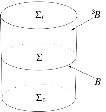
Figure 1. Finite spacetime domain $\mathcal{M}\subset\mathbb{E}^{3}$ with boundary $\partial\mathcal{M}=\Sigma_{0}\cup\Sigma_{F}\cup{}^{3}\!B$. Respectively, $\Sigma_{0}$ and $\Sigma_{F}$ denote the solid round ball $\Sigma$ at the initial time $t_{0}$ and the final time $t_{F}$. Radiation boundary conditions are given on the three–dimensional timelike cylinder ${}^{3}\!B$. Our geometric perspective on the “quasilocal” spacetime region $\mathcal{M}$ comes from Refs. [2] and [3].

More generally, one might consider radiation boundary conditions associated with some other pde and/or different type of $B$ boundary, say cubical or irregularly shaped. Refs. [4] through [20] pertain either to the described spherical problem or to more general radiation boundary conditions. This is certainly not an exhaustive list, and we point the reader to review articles [11, 17, 20] for more comprehensive listings. Although we do not attempt an extensive literature review, we make mention of a few approaches to radiation boundary conditions in order to put our work in some context. Two pioneering early works are those of Engquist and Majda [5, 6] and Bayliss and Turkel [8]. Each develops a hierarchy of local differential conditions of increasing complexity. Engquist and Majda’s work is based on exact radiation boundary conditions as expressed within the theory of pseudo–differential operators, and their approach is not necessarily tied to a spherical geometry nor to the ordinary wave equation. Also considering more than just our problem above, Bayliss and Turkel base their approach on asymptotic expansions about infinity, for example the standard multipole expansion for a radiating field obeying the ordinary wave equation (1). Another approach to radiation boundary conditions relies on the introduction of absorbing layers, and as an example we mention Ref. [10]. In the introduction of his review article [17], Hagstrom describes the main advances made in the 1990s on several fronts related to radiation boundary conditions: (i) improved implementations of hierarchies, such as the ones mentioned, (ii) new absorbing layer techniques exhibiting reflectionless interfaces, and (iii) efficient algorithms for evaluation of exact nonlocal boundary operators. Results [14, 15, 16] of Grote and Keller fall within this first category. An advance on the second front was the introduction of perfectly matched layers by Bérenger [13], while a key advance on the third was the rapid implementation of nrbc for spherical boundaries by Alpert, Greengard, and Hagstrom [18, 19]. See also related work by Sofronov [12]. Hagstrom discusses the state of the art for both fronts (ii) and (iii) in his second review article [20].

0.2. Alpert, Greengard, Hagstrom nonreflecting boundary conditions

Since our investigation will follow the approach of Alpert, Greengard, and Hagstrom (agh) which belongs to category (iii) in the last paragraph, let us describe it in more detail. With $U_{lm}(t,r)$ denoting a single spherical harmonic mode of the wave field ($l$ and $m$ are the standard orbital and azimuthal integers), we consider the reduced ordinary $3+1$ wave equation,

(2) $$\frac{\partial^{2}U_{l}}{\partial t^{2}}-\frac{\partial^{2}U_{l}}{\partial r^{2}}-\frac{2}{r}\frac{\partial U_{l}}{\partial r}+\frac{l(l+1)}{r^{2}}U_{l}=0,$$

stemming from the (1). We have dropped the index $m$ on $U_{l}$ since it does not appear in the pde. Let $\hat{U}_{l}(s,r)=\mathcal{L}[U_{l}](s,r)$ denote the Laplace transform of the mode. Provided that we assume both compactly supported initial data and a large enough radius $r$, the transform $\hat{U}_{l}(s,r)$ obeys a homogeneous ode,

(3) $$z^{2}\frac{\mathrm{d}^{2}\hat{U}_{l}}{\mathrm{d}z^{2}}+2z\frac{\mathrm{d}\hat{U}_{l}}{\mathrm{d}z}-\left[z^{2}+l(l+1)\right]\hat{U}_{l}=0\,,$$

known as the modified spherical Bessel equation. Here $z=sr$ is shorthand for the product of Laplace frequency $s$ and radius $r$. In terms of the standard half–integer order MacDonald function [21] $K_{l+1/2}(z)$, we define an associated function $W_{l}(z)=(\pi z/2)^{1/2}\exp(z)K_{l+1/2}(z)$ more closely related to a confluent hypergeometric function. The function $z^{-1}\exp(-z)W_{l}(z)$ is the outgoing solution to (3). Here $W_{l}(z)$ has been chosen so that $W_{l}(z)\sim 1$ as $z\rightarrow\infty$, that is “normalized at infinity.” Moreover, it turns out that $W_{l}(z)$ is a polynomial of degree $l$ in inverse $z$. For example, $W_{0}(z)=1$, $W_{1}(z)=1+z^{-1}$, $W_{2}(z)=1+3z^{-1}+3z^{-2}$.

agh introduce a nonreflecting boundary kernel, here called a time–domain radiation kernel (tdrk) as follows. Again assuming compactly supported initial data and a large enough radial value, the Laplace transform of the mode $U_{l}(t,r)$ takes the form

(4) $$\hat{U}_{l}(s,r)=a_{l}(s)r^{-1}\exp(-sr)W_{l}(sr)\,,$$

where $a_{l}(s)$ is an analytic function of $s$ depending on the details of the initial data. Differentiation of the last equation with respect to $r$ leads to the identity (the prime denotes differentiation in argument)

(5) $$s\hat{U}_{l}(s,r)+\partial_{r}\hat{U}_{l}(s,r)+r^{-1}\hat{U}_{l}(s,r)=r^{-1}\big{[}srW_{l}^{\prime}(sr)/W_{l}(sr)\big{]}\hat{U}_{l}(s,r)\,.$$

This identity is of course valid at the fixed outer boundary radius $r_{B}$, provided that the outer two–sphere boundary $B$ lies beyond the support of the initial data. A well–known classical result, $W_{l}(z)$ has $l$ simple zeros $\{k_{l,n}:n=1,\cdots,l\}$ which lie in the lefthalf plane. The $k_{l,n}$ are also the zeros of $K_{l+1/2}(z)$, as discussed in [18] and below. As a result, the object $\hat{\omega}_{l}(s;r_{B})=sr_{B}W_{l}^{\prime}(sr_{B})/W_{l}(sr_{B})$, a frequency–domain radiation kernel (fdrk), is a sum of $l$ simple poles in the lefthalf $s$–plane,

(6) $$\hat{\omega}_{l}(s;r_{B})=\sum_{n=1}^{l}\frac{k_{l,n}/r_{B}}{s-k_{l,n}/r_{B}}\,.$$

Whence its inverse Laplace transform $\omega_{l}(t;r_{B})$, the tdrk of agh, is a corresponding sum of exponentials,

(7) $$\omega_{l}(t;r_{B})=\sum_{n=1}^{l}(k_{l,n}/r_{B})\exp\big{(}k_{l,n}t/r_{B}\big{)}\,.$$

We find the following for the first three such kernels:

(8) $$\omega_{0}(t;r_{B}) =0\,,$$

$$\omega_{1}(t;r_{B}) =-r_{B}^{-1}\exp\big{(}-t\big{/}r_{B}\big{)}\,,$$

$$\omega_{2}(t;r_{B}) =-r_{B}^{-1}\exp\big{(}-{\textstyle\frac{3}{2}}t/r_{B}\big{)}\big{[}3\cos\big{(}{\textstyle\frac{1}{2}}\sqrt{3}t/r_{B}\big{)}+\sqrt{3}\sin\big{(}{\textstyle\frac{1}{2}}\sqrt{3}t/r_{B}\big{)}\big{]}\,.$$

By elementary properties of the Laplace transform, including the Laplace convolution theorem, inverse transformation of the identity (5) yields the following robc (a condition of complete transparency):

(9) $$\left.\left[\frac{\partial U_{l}}{\partial t}+\frac{\partial U_{l}}{\partial r}+\frac{U_{l}}{r}\right]\right|_{r=r_{B}}=r^{-1}_{B}\int_{0}^{t}\omega_{l}(t-t^{\prime};r_{B})U_{l}(t^{\prime},r_{B}){\rm d}t^{\prime}\,.$$

From a numerical standpoint, this boundary condition becomes expensive for high–order modes, since $\omega_{l}(t;r_{B})$ is made up of $l$ exponential factors. However, elementary exponential identities do afford an efficient recursive evaluation of the convolution [18]. For wave propagation on flat 2+1 spacetime, the analogous cylindrical tdrk for a given angular mode is again a sum of exponentials, but now the sum is over a set including a continuous sector [18]. Remarkably, this is a feature shared by blackhole kernels. Such continuous distributions are primarily relevant for the low–order modes and quite expensive to evaluate.

agh describe an algorithm for kernel compression, by which we mean approximation of the fdrk by a rational function, where the approximation is of specified relative error $\varepsilon$ uniformly for $\mathrm{Re}s\geq 0$. The resulting rational function, itself a sum of simple poles, typically involves far fewer terms. As a result, in the agh approach the cost of updating the numerical solution at the outer boundary $B$ is minimized subject to the prescribed tolerance $\varepsilon$ (which also turns out to be a relevant error measure in the time–domain). Therefore, we may describe their implementation of robc for the ordinary wave equation as rapid. agh have given a formidable asymptotic analysis of their rapid implementation, proving in particular that the number $d$ of poles needed to approximate the fdrk to within the specified tolerance scales like

(10) $$d\sim O\big{(}\log\nu\log(1/\varepsilon)+\log^{2}\nu+\nu^{-1}\log^{2}(1/\varepsilon)\big{)}$$

as $\nu=l+1/2\rightarrow\infty$ and $\varepsilon\rightarrow 0^{+}$ [18]. Increased performance as $\nu\rightarrow\infty$ is also seen for rational approximation of the cylindrical kernels relevant for 2+1 wave propagation. However, as remarked upon later in Section 3.3.1, for both the 2+1 and blackhole scenarios rational approximation of low–order kernels (associated with costly continuous sectors) also leads to savings.

0.3. Problem statement

Now consider the evolution problem for the scalar wave equation,

(11) $$\sum_{\mu,\nu=0}^{3}\frac{1}{\sqrt{-g}}\frac{\partial}{\partial x^{\mu}}\left(\sqrt{-g}g^{\mu\nu}\frac{\partial U}{\partial x^{\nu}}\right)=0\,,$$

describing a field $U$ propagating on a Schwarzschild blackhole determined by $g_{\mu\nu}$ metric functions. A slight modification of (11) yields a wave equation flexible enough to also describe propagation of electromagnetic or gravitational waves on a Schwarzschild blackhole [23, 24, 25, 26]. As a model of gravitational wave propagation, the problem has applications in relativistic astrophysics: non–spherical gravitational collapse and stellar perturbations, among others. Gravitational wave propagation is also of considerable theoretical interest in general relativity. With numerical wave simulation on a finite mesh in mind, we again choose a finite domain $\Sigma$, now a round, three–dimensional, thick shell also bounded internally by the blackhole horizon $H$. The outer boundary $B$, one element of $\partial\Sigma=B\cup H$, is again specified by $r=r_{B}$, while the inner boundary $H$ corresponds to $r=2{\rm m}$ (twice the geometrical mass of the blackhole). Let us set the task of evolving data $U|_{t_{0}}$ and $\partial_{t}U|_{t_{0}}$ given on $\Sigma_{0}$, in order to generate the solution $U$ on the finite domain $\mathcal{M}=[t_{0},t_{F}]\times\Sigma$ with boundary $\partial\mathcal{M}=\Sigma_{0}\cup\Sigma_{F}\cup{}^{3}\!B\cup{}^{3}\!H$. Here ${}^{3}\!H$, a portion of the future event horizon, is the three–dimensional characteristic history $[t_{0},t_{F}]\times H$ of $H$. To accomplish the task, we need explicit outer boundary conditions on ${}^{3}\!B=[t_{0},t_{F}]\times B$, ones stemming from the assumption of trivial initial data on the outer spatial region exterior to $\Sigma_{0}$. We refer to these as radiation outer boundary conditions (robc). The robc corresponding to (11) are more subtle than simple nonreflection, in part due to the back–scattering of waves off of curvature.

In discussing finite outer boundary conditions, and robc in particular, for relativity, we should first make a distinction between general relativity, in which the dynamics of spacetime is governed by the full nonlinear Einstein equations, and its perturbation theory, in which the dynamics of disturbances on a fixed background solution to the Einstein equations is governed by a linear pde similar to (11). In this second paradigm one examines the propagation of weak gravitational waves on a fixed background spacetime (which may or may not be curved). York’s survey article [27] on the dynamics and kinematics of general relativity is the best jumping off point for a study of the literature we now mention. Within the context of a mixed Cauchy–boundary value problem, Friedrich and Nagy have made theoretical progress towards solving the full Einstein equations on a bounded domain [28]; however, their results do not appear suited for numerical work. For the most part, approaches towards numerical outer boundary conditions in the full theory have relied either on matching Cauchy domains to characteristic surfaces (see [29, 30] and references therein) or ensuring that the outer boundary is at a large enough distance so that perturbation theory can be brought into play (see [31, 32] and reference therein). In this latter approach, the relevant perturbative wave equation is essentially (11); however, the corresponding exact nonlocal robc are not used. A very different approach towards theoretical and numerical outer boundary conditions has been given in [33]. However, it would seem of limited practical use, since it relies on the “many–fingered” nature of time in general relativity to completely freeze the flow of time at the outer boundary. In terms of harmonic coordinates Szilágyi, Schmidt, and Winicour have theoretically and numerically studied mixed Cauchy–boundary value problems for the Einstein equations linearized about flat Minkowski spacetime [34]. Attempts towards implementation of robc in numerical relativity have mostly relied on improved versions of the well–known Sommerfeld condition, although Novak and Bonazzola have considered more general nonreflecting boundary conditions with relativistic applications in mind [35]. The Sommerfeld condition is a local boundary condition which is exact for a spherically symmetric outgoing wave in flatspace. Recently, Allen, Buckmiller, Burko, and Price have discussed the effect of such approximate boundary conditions on long–time numerical simulation of waves on the Schwarzschild geometry [36] (we consider one of their numerical experiments below). For comments on such approaches as well as other remarks on numerical relativity, see the review article by Cook and Teukolsky [37]. To date, there seems to have been no truly systematic analysis of algorithm error for treatments of robc in numerical relativity.

We use frequency–domain methods and gather results which resemble those used and found in seminal work [38] by Leaver and also in related work [39] by Andersson. Despite this resemblance, neither Leaver nor Andersson considered boundary integral kernels belonging to the finite timelike cylinder ${}^{3}\!B$. The starting point for these authors was the exact solution to the Cauchy problem as expressed via an integral (Green’s function) representation involving $\Sigma_{0}$ spatial convolution with initial data (actually Leaver also considered more general driving source terms beyond just initial data). As Leaver noted in footnote 21 of [38], the seeds of this approach are found in Morse and Feshbach’s 1953 treatment [40] of the ordinary flatspace wave equation, although they have origins in the 19th century. Many authors have since used frequency–domain and complex–analytic methods to examine the Cauchy problem for perturbations on the Schwarzschild geometry from this Green’s function perspective, and Andersson’s article [39] is a salient recent example. However, we stress up–front that our problem of imposing robc via domain reduction is not the same as Leaver and Andersson’s problem, and our work has quite a different focus on ${}^{3}\!B$ temporal integral convolution. Moreover, the methods —those of agh— that we describe and use in this article and its follow–up were only fully developed for the ordinary wave equation in the late 1990s. Section 1.4.3 further compares and contrasts our theoretical analysis with that of Leaver and Andersson.

0.4. Overview of results

In this article we describe both the exact robc for (11) and an algorithm for their rapid numerical implementation. As mentioned, our approach to the problem follows agh quite closely. The equation (11) is linear, but necessarily with variable coefficients. Nevertheless, exploiting its time and rotational symmetries, we may likewise use Laplace and spherical–harmonic transformation in order to obtain a second–order radial ode which turns out to be an incarnation of the confluent Heun equation [41, 42], also related to the generalized spheroidal wave equation discussed in some literature [43, 44]. Following agh, we may formally introduce the tdrk as the inverse Laplace transform of the homogeneous logarithmic derivative of the asymptotically outgoing solution. Analytically, the fdrk, the logarithmic derivative in question, is a sum of poles, although now the sum is over both a discrete set and a continuous set (similar to the situation for the flatspace wave equation in $2+1$ rather than 3+1 dimensions [18]).

Employing both direct numerical construction of blackhole fdrk’s as well as their compression along the lines of agh, we numerically implement the exact robc for waves on Schwarzschild. In principle, we may implement the conditions to arbitrary numerical accuracy even for long–time simulations. Via study of one–dimensional radial evolutions, we demonstrate that the described robc capture the long–studied phenomena of both quasinormal ringing and late–time decay tails. Since our implementation is based on the exact nonlocal history–dependent robc, we sidestep issues raised by Allen, Buckmiller, Burko, and Price [36] and are indeed able to capture decay tails with our boundary conditions. We demonstrate this below with an example considered in [36]. We also consider a three–dimensional evolution based on a spectral code, one showing that the robc yield accurate results for the scenario of a wave packet striking the boundary at an angle. Our work is a partial generalization to Schwarzschild wave propagation and Heun functions of the methods developed for flatspace wave propagation and Bessel functions by agh, save for one key difference. Whereas agh had the usual armamentarium of analytical results (asymptotics, order recursion relations, bispectrality) for Bessel functions at their disposal, what we need to know about Heun functions must be gathered numerically as relatively less is known about them.

Due to this key difference, we are, unfortunately, unable to offer a rigorous asymptotic analysis of our rapid implementation. However, our numerical work suggests that the number $d$ of approximating poles grows at a rate not at odds with the one mentioned above. Indeed, as seen in Table 5 from Section 3.3.1, for $\varepsilon=10^{-10}$ and $r_{B}=30\mathrm{m}$ we have found that $d=20$ is sufficient for all $l\leq 64$. With the same $r_{B}$ but $\varepsilon=10^{-6}$ instead, $d=14$ is sufficient for all $l\leq 256$. These $d$ values gives us some idea of the cost associated with our rapid implementation. Let us focus attention on a single spherical harmonic mode, ignoring the cost of performing a (numerical) harmonic transform. Depending on the algorithm used for wave simulation, such a transform may or may not be performed at each numerical time step. For the range of $l$ values and $\varepsilon$ accuracies we consider, $d$ is roughly on the order of 10. Therefore, at each numerical time step we expect a boundary operation count which is some multiple $10p$ of this $d$ value. (Actually poles whose locations are properly complex are more costly than those which lie on the real axis. This affects $p$, but no matter.) A practical radial discretization of $[2\mathrm{m},30\mathrm{m}]$ will have some multiple $1000q$ of a thousand mesh points, whence $p/q$ is a straightforward estimate for the percentage cost (at each numerical time–step) of updating the solution at the edge of the computational domain relative to the cost of updating on the interior. Note that while $p$ remains fixed, $q$ increases with mesh resolution, so that the cost of our robc relative to interior cost becomes accordingly negligible. Let us support this assertion with a concrete example. For the one–dimensional radial evolution described in Section 5.1.1, we have kept track of the total cpu time spent both on interior work and the robc. We list the ratio of these times as percentages in Table 1. Such percentages belie the true savings of the implementation. Without some form of robc, one would be forced to consider the free evolution of waves on a domain larger than $[2\mathrm{m},30\mathrm{m}]$, one large enough to ensure that the waves would not reach the larger outer boundary during the simulation. The cost of using a larger domain as “boundary conditions” is usually some multiple of the interior cost. Therefore, our robc typically cost less than a percent of what evolution on such a larger domain costs. In Section 4.3.3 we discuss memory and storage issues relevant to our implementation of robc.

	Number of radial mesh points
$l$	1024	2048	4096	8182	16384
$0$	2.24	1.49	1.00	0.39	0.21
$33$	2.41	1.76	1.31	0.50	0.26
$64$	2.55	1.81	1.37	0.51	0.27

Table 1. Relative cost of $\varepsilon=10^{-10}$ robc. For the one–dimensional evolution described in Section 5.1.1, we list percentage values for cpu time spent on robc relative to cpu time spent on interior work. Whence each value is essentially the aforementioned ratio $p/q$ for a particular $q$.

0.5. Summary

Section 1 discusses variable transformations, various resulting forms of (11), and the exact robc. We start off by defining dimensionless coordinates for time $\tau$, radius $\rho$, and Laplace frequency $\sigma$. For example, $r=2{\rm m}\rho$ and $s=\sigma/(2{\rm m})$. The outer boundary $B$ is determined $\rho=\rho_{B}$. With these coordinates we introduce the asymptotically outgoing solution $W_{l}(\sigma\rho;\sigma)$ to the radial equation, the one corresponding to the Bessel–type function $W_{l}(sr)=W_{l}(\sigma\rho)$ above. For a given angular index $l$ the tdrk $\omega_{l}(\tau;\rho_{B})$ is the inverse Laplace transform of the fdrk $\hat{\omega}_{l}(\sigma;\rho_{B})=\sigma\rho_{B}W_{l}^{\prime}(\sigma\rho_{B};\sigma)/W_{l}(\sigma\rho_{B};\sigma)$. We then write the robc as an integral convolution between $\omega_{l}(\tau;\rho_{B})$ and each of the corresponding $2l+1$ modes $\psi_{lm}(\tau,\rho_{B})$ of the radiating field $\psi(\tau,\rho,\theta,\phi)$, where $\psi$ is $U$ from above but expressed in terms of different coordinates. Afterwards, we describe the key representation of $\hat{\omega}_{l}(\sigma;\rho_{B})$ as a (continuous and discrete) sum of poles. Section 1 ends with the derivation of an estimate for the relative error $\varepsilon$ associated with approximating $\omega_{l}(\tau;\rho_{B})$ by a numerical kernel $\xi_{l}(\tau;\rho_{B})$.

Section 2 describes numerical evaluation of both $W_{l}(\sigma\rho_{B};\sigma)$ and $\hat{\omega}_{l}(\sigma;\rho_{B}$), with the former considered as a function of complex Laplace frequency $\sigma$ (mostly lying in the lefthalf plane) and the latter as a function of purely imaginary $\sigma={\rm i}y$. Both types of evaluation rely on numerical integration over certain paths in the complex plane. We consider several numerical methods, but the main ones involve path integration in terms of a complex variable $z=\sigma\rho$. While numerical evaluation of $W_{l}(\sigma\rho_{B};\sigma)$ is important insofar as studying the analytic structure of this function is concerned, implementation of robc mainly requires that we are able to accurately evaluate $\hat{\omega}_{l}({\rm i}y;\rho_{B})$ for any $y\in\mathbb{R}$. In this section we also discuss in detail the accuracy of our numerical methods.

Section 3 focuses on the sum–of–poles representations of $\hat{\omega}_{l}(\sigma;\rho_{B})$. The first subsection is a qualitative description of the analytic structure of $W_{l}(\sigma\rho_{B};\sigma)$ and its relevance for the exact sum–of–poles representation. This subsection examines the zeros in frequency $\sigma$ of $W_{l}(\sigma\rho_{B};\sigma)$ which correspond to poles of $\hat{\omega}_{l}(\sigma;\rho_{B})$. It also studies the branch behavior of $W_{l}(\sigma\rho_{B};\sigma)$ along the negative Re$\sigma$ axis, behavior that gives rise to a continuous pole distribution (these are not really poles in the sense of complex analysis). This distribution appears in the exact sum–of–poles representation, and we graphically examine it. The second subsection presents our direct numerical construction of $\hat{\omega}_{l}(\sigma;\rho_{B})$ for $0\leq l\leq 10$ and $\rho_{B}\in[15,25]$. We discuss several numerical accuracy checks of our direct construction. The third describes kernel compression, and the resulting approximation of $\hat{\omega}_{l}(\sigma;\rho_{B})$ by a rational function which is itself a sum of poles. In this third subsection we consider the bandwidth $0\leq l\leq 64$.

Section 4 presents the details of our implementation of robc. As mentioned, our implementation is designed around the MacCormack predictor–corrector algorithm [45]. The first subsection describes both our choice of spacetime foliation and the associated first–order evolution system of pde, while the second reviews the MacCormack algorithm in the context of this system. As an aside, the second subsection also addresses the issue of inner boundary conditions at the horizon $H$. The third subsection describes the implementation, showing how robc fit within the framework of the interior prediction and correction. In this final subsection we also address some memory issues relevant to our implementation.

Section 5 documents the results of several numerical tests of our implementation of robc. Throughout this section, we consider a blackhole of mass $\mathrm{m}=2$ enclosed within an outer boundary of radius $r_{B}=60$ so that the horizon is located at $2\mathrm{m}=4$ and $\rho_{B}=15$. The choice $\mathrm{m}=2$ is not particularly special, and has been made only to provide an example in which the mass is neither $\frac{1}{2}$ nor $1$. The bulk of this section focuses on one–dimensional radial evolutions of single spherical–harmonic modes. However, in the last subsection we consider a three–dimensional test.

A final sections offers some conclusions and also discusses applications and extensions of our results.

In Appendix A we discuss a certain modification of the MacCormack algorithm which is featured in our implementation of robc. In Appendix B we provide numerical tables for several compressed kernels.

Starting on page  we have listed our main symbols in order of appearance, with the section number given for where each symbol first appears. Symbols not listed there are defined and used locally. Although some symbols in this work have multiple meanings, within a given section a symbol’s meaning does not change. We point out that as a complex variable $\sigma=x+\mathrm{i}y$, and, therefore, for the complex variable $z=\sigma\rho$ we always write $z=\mathrm{Re}z+\mathrm{i}\mathrm{Im}z$.

1. Wave equation and radiation outer boundary conditions

This section sets up the theoretical framework on which the subsequent sections rest. We here discuss various pde and ode relevant for wave propagation on the Schwarzschild geometry. We then derive the exact and nonlocal radiation outer boundary conditions (robc) appropriate for asymptotically outgoing fields, thereby paving the way for their numerical implementation in later sections.

1.1. Wave equation on Schwarzschild background

1.1.1. Line–element

Consider the diagonal line–element describing a static, spherically symmetric, vacuum blackhole of mass $\mathrm{m}$,

(12) $$\mathrm{d}s^{2}=-F\mathrm{d}T^{2}+F^{-1}\mathrm{d}r^{2}+r^{2}\mathrm{d}\theta^{2}+r^{2}\sin^{2}\theta\mathrm{d}\phi^{2}\,,$$

written with respect to the standard static time $T$ and areal radius $r$ [52, 53]. We use uppercase $T$ here to save lowercase $t$ for a different time coordinate needed later. Note that the metric coefficient $F(r)=1-2\mathrm{m}/r$ vanishes —and so $F^{-1}$ is singular— as $r\rightarrow 2\mathrm{m}$. As is well known, $r=2\mathrm{m}$ does not represent a physical singularity, rather the coordinate system is degenerate for this value of the radius. In these coordinates the round sphere determined by $r=2\mathrm{m}$ is the bifurcate cross–section of the event horizon of the blackhole. In this work, we are chiefly interested in the “exterior region” defined by $2\mathrm{m}<r<\infty$.

It will prove convenient to pass to and work with dimensionless coordinates $(\tau,\rho,\theta,\phi)$ defined by

(13) $$2\mathrm{m}\tau=T\,,\quad 2\mathrm{m}\rho=r$$

($\theta$ and $\phi$ are already dimensionless). After the rescaling $\mathrm{d}s^{2}\mapsto\mathrm{d}s^{2}/(4\mathrm{m}^{2})$, we may rewrite the line–element (12) in the dimensionless form

(14) $$\mathrm{d}s^{2}=-F\mathrm{d}\tau^{2}+F^{-1}\mathrm{d}\rho^{2}+\rho^{2}\mathrm{d}\theta^{2}+\rho^{2}\sin^{2}\theta\mathrm{d}\phi^{2}\,,$$

where now $F(\rho)=1-1/\rho$ so the unphysical singularity is located at $\rho=1$.

We also consider the outgoing and ingoing systems of Eddington–Finkelstein coordinates [52, 53], here in dimensionless form. To construct them, first introduce the Regge–Wheeler tortoise coordinate [24, 52]

(15) $$\rho_{*}=\rho+\log(\rho-1)\,.$$

Recall that this transformation is valid for $1<\rho<\infty$ which corresponds to $-\infty<\rho_{*}<\infty$, and that $\rho\rightarrow 1^{+}$ corresponds to $\rho_{*}\rightarrow-\infty$. In terms of the tortoise coordinate we write (14) as

(16) $$\mathrm{d}s^{2}=F\big{(}-\mathrm{d}\tau^{2}+\mathrm{d}\rho_{*}^{2}\big{)}+\rho^{2}\mathrm{d}\theta^{2}+\rho^{2}\sin^{2}\theta\mathrm{d}\phi^{2}\,.$$

The characteristic coordinate $\mu=\tau-\rho_{*}$ is the retarded time, and the set $(\mu,\rho,\theta,\phi)$ is the outgoing Eddington–Finkelstein system. With respect to it, the line–element takes the form

(17) $$\mathrm{d}s^{2}=-F\mathrm{d}\mu^{2}-2\mathrm{d}\mu\mathrm{d}\rho+\rho^{2}\mathrm{d}\theta^{2}+\rho^{2}\sin^{2}\theta\mathrm{d}\phi^{2}\,.$$

In the $(\mu,\rho,\theta,\phi)$ system $g_{\rho\rho}=0$, so that the vector field $\partial/\partial\rho$ is characteristic or null, whereas in the $(\tau,\rho,\theta,\phi)$ system $g_{\rho\rho}=F^{-1}(\rho)$, so that $\partial/\partial\rho$ is spacelike on the exterior region. Level–$\mu$ hypersurfaces are characteristic and outgoing (cones which open up towards the future) with $\partial/\partial\rho$ as their outgoing generator. In Section 4.1.1 we consider the ingoing Eddington–Finkelstein coordinate system which is based on the characteristic coordinate $\nu=\tau+\rho_{*}$ known as advanced time.

1.1.2. Wave equation

The covariant d’Alembertian or wave equation associated with the diagonal line–element (14) is the following:

(18) $$\left(1-\frac{1}{\rho}\right)^{-1}\frac{\partial^{2}\psi}{\partial\tau^{2}}-\frac{1}{\rho^{2}}\frac{\partial}{\partial\rho}\left[\rho^{2}\left(1-\frac{1}{\rho}\right)\frac{\partial\psi}{\partial\rho}\right]-\frac{\Delta_{S^{2}}\psi}{\rho^{2}}=0\,,$$

where $\Delta_{S^{2}}$ is the Laplace operator (with negative eigenvalues) belonging to the unit–radius round sphere $S^{2}$. Notice that we use $\psi$ for the wave field associated with the static time coordinate $\tau$ (or associated with its counterpart $T$) introduced above, whereas in the introduction we have used $U$ for the wave field. Later we use $U$ for the wave field associated with a certain time variable $t$ related to ingoing Eddington–Finkelstein coordinates. Our numerical work is based on $t$ (which is why $U$ and $t$, rather than $\psi$ and $T$, appear in the introduction). For flat spacetime $T$ and $t$ are the same, and so $\psi$ and $U$ are also formally the same for $\mathrm{m}=0$.

Introducing the standard set $Y_{lm}(\theta,\phi)$ of basis functions for square–integrable functions on $S^{2}$, we consider an appropriate expansion

(19) $$\psi(\tau,\rho,\theta,\phi)=\sum_{l,m}\psi_{lm}(\tau,\rho)Y_{lm}(\theta,\phi)$$

of the field $\psi$ in terms of spherical–harmonic modes $\psi_{lm}$. The spherical–harmonic transform of (18),

(20) $$\left(1-\frac{1}{\rho}\right)^{-1}\frac{\partial^{2}\psi_{l}}{\partial\tau^{2}}-\frac{1}{\rho^{2}}\frac{\partial}{\partial\rho}\left[\rho^{2}\left(1-\frac{1}{\rho}\right)\frac{\partial\psi_{l}}{\partial\rho}\right]+\frac{l(l+1)\psi_{l}}{\rho^{2}}=0\,,$$

is the pde governing the evolution of a generic mode $\psi_{l}$. On $\psi_{l}$ we have suppressed the $m$, since it does not appear in the pde.

Addition of a single simple term to (20) yields a modified wave equation flexible enough to describe either the mode evolution of an electromagnetic field $A_{\beta}$ or the mode evolution of small gravitational perturbations $\delta g_{\alpha\beta}$ on the Schwarzschild background. The modified equation is

(21) $$\left(1-\frac{1}{\rho}\right)^{-1}\frac{\partial^{2}\psi_{l}}{\partial\tau^{2}}-\frac{1}{\rho^{2}}\frac{\partial}{\partial\rho}\left[\rho^{2}\left(1-\frac{1}{\rho}\right)\frac{\partial\psi_{l}}{\partial\rho}\right]+\frac{l(l+1)\psi_{l}}{\rho^{2}}-\frac{\jmath^{2}\psi_{l}}{\rho^{3}}=0$$

with the spin $\jmath=0,1,2$ corresponding to scalar, electromagnetic, and gravitational radiation. We review the history of this correspondence in the next paragraph. We may cast (21) in a particularly simple form via simultaneous transformation of the independent and dependent variables. Indeed, setting $\Psi_{l}=\rho\psi_{l}$ and here viewing $\partial/\partial\rho_{*}$ as shorthand for $(1-\rho^{-1})\partial/\partial\rho$, we rewrite (21) as follows:

(22) $$\frac{\partial^{2}\Psi_{l}}{\partial\tau^{2}}-\frac{\partial^{2}\Psi_{l}}{\partial\rho^{2}_{*}}+V(\rho)\Psi_{l}=0\,.$$

The Regge–Wheeler potential

(23) $$V(\rho)=\left(1-\frac{1}{\rho}\right)\left[\frac{l(l+1)}{\rho^{2}}+\frac{1-\jmath^{2}}{\rho^{3}}\right]$$

would depend only implicitly on $\rho_{*}$ were we using $\rho_{*}$ as the independent variable. As we will see in Section 1.2.3, the Laplace transform of (22) is important theoretically, since it elucidates the role of Laplace frequency as a spectral parameter.

Wheeler derived the $j=1$ version of (22,23) in 1955 [23], showing that each of the two polarization states for an electromagnetic field on the Schwarzschild geometry is described by one copy of the equation. Regge and Wheeler then derived the $\jmath=2$ equation for odd–parity (or axially) gravitational perturbations in 1957 [24], and Zerilli introduced a similar equation describing even–parity (or polar) gravitational perturbations in 1970 [25]. In the 1970s Chandrasekhar and Detweiler demonstrated that the Zerilli equation can be derived from (22), although the derivation involves differential operations (see [26] and references therein).

Adopting $\mu$ as the time coordinate, we define $\varphi_{l}(\mu,\rho)=\psi_{l}(\mu+\rho_{*},\rho)$ and write (21) as

(24) $$2\frac{\partial^{2}\varphi_{l}}{\partial\mu\partial\rho}+\frac{2}{\rho}\frac{\partial\varphi_{l}}{\partial\mu}-\frac{1}{\rho^{2}}\frac{\partial}{\partial\rho}\left[\rho^{2}\left(1-\frac{1}{\rho}\right)\frac{\partial\varphi_{l}}{\partial\rho}\right]+\frac{l(l+1)\varphi_{l}}{\rho^{2}}-\frac{\jmath^{2}\varphi_{l}}{\rho^{3}}=0\,.$$

Another way to obtain this wave equation is to form the d’Alembertian associated with (17) and then implement a spherical–harmonic transformation. Similar to above, we may either set $\Phi_{l}=\rho\varphi_{l}$ or $\Phi_{l}(\mu,\rho)=\Psi_{l}(\mu+\rho_{*},\rho)$, thereby expressing (22) as

(25) $$2\frac{\partial^{2}\Phi_{l}}{\partial\mu\partial\rho_{*}}-\frac{\partial^{2}\Phi_{l}}{\partial\rho^{2}_{*}}+V(\rho)\Phi_{l}=0\,,$$

again viewing $\partial/\partial\rho_{*}$ as a shorthand. As we will see, for a given $l$ the fdrk is built from the outgoing solution to the formal Laplace transform of (25). Table 2 lists the wave fields we have introduced, and it also briefly describes the theoretical importance of each field’s Laplace transform. The statements made in the table are explained in Sections 1.2 and 1.3.

Static time coordinate system $(\tau,\rho)$		Retarded time coordinate system $(\mu,\rho)$
$\psi_{l}(\tau,\rho)$	ode for L.t. is analogous to	$\varphi_{l}(\mu,\rho)$	$\jmath=0$ ode for L.t. is directly
	the spherical Bessel equation.		the confluent Heun equation.
$\Psi_{l}(\tau,\rho)$	ode for L.t. elucidates role	$\Phi_{l}(\mu,\rho)$	ode for L.t. has outgoing
	of $\sigma$ as a spectral parameter.		solution normalized at $\infty$.

Table 2. Wave fields and their relevance. L.t. stands for Laplace transform. As we discuss in Section 1.2, via the Laplace transform we trade a pde for an ode.

1.2. Laplace transform and radial wave equation

1.2.1. Laplace transform

The Schwarzschild geometry is static, and with respect to the chosen coordinates we indeed see that the components of the metric tensor are $\tau$–independent. In turn, the variable coefficients of the linear wave equation described in the last subsection do not depend on time, a scenario permitting study of the equation via the technique of Laplace transform. The description of the technique in Chapter 12 of the textbook [55] by Greenberg is suitable for our purposes. Let $\mathcal{L}$ denote the transform operation,

(26) $${\mathcal{L}}[g](\sigma)=\int^{\infty}_{0}e^{-\sigma\tau}g(\tau){\rm d}\tau\,.$$

Here we use $\sigma$ for the variable dual to $\tau$ with respect to the Laplace transform. We may define a physical variable $s=\sigma/(2\mathrm{m})$, with dimensions of inverse length, which is dual to $t$ and satisfies $st=\sigma\tau$. We may also define a formal Laplace transformation on the retarded time $\mu$ by replacing $\tau$ with $\mu$ in the last equation. For the time being we proceed with the transformation on $\tau$.

1.2.2. Laplace transform of the wave equation

Let us formally compute the Laplace transform of (21), in order to get an ode in the radial variable $\rho$. With $\hat{\psi}_{l}={\mathcal{L}}[\psi_{l}]$ and a dot denoting $\tau$ differentiation, we have

$${\mathcal{L}}[\dot{\psi}_{l}](\sigma,\rho) =\sigma\hat{\psi}_{l}(\sigma,\rho)-\psi_{l}(0,\rho)\,,$$

(27) $${\mathcal{L}}[\ddot{\psi}_{l}](\sigma,\rho) =\sigma^{2}\hat{\psi}_{l}(\sigma,\rho)-\sigma\psi_{l}(0,\rho)-\dot{\psi}_{l}(0,\rho)\,,$$

provided $\mathrm{Re}\sigma>0$. We assume that the initial data $\psi_{l}(0,\rho)$ and $\dot{\psi}_{l}(0,\rho)$ vanish in a neighborhood of $\rho$, as is true for compactly supported data so long as we choose $\rho$ large enough. This assumption ensures formally that upon Laplace transformation we may replace $\tau$ partial differentiation by $\sigma$ multiplication. Whence, after some simple algebra we find

(28) $$\frac{\mathrm{d}^{2}\hat{\psi}_{l}}{\mathrm{d}\rho^{2}}+\frac{2\rho-1}{\rho(\rho-1)}\frac{\mathrm{d}\hat{\psi}_{l}}{\mathrm{d}\rho}+\left[\frac{-\sigma^{2}\rho^{2}}{(\rho-1)^{2}}-\frac{l(l+1)}{\rho(\rho-1)}+\frac{\jmath^{2}}{\rho^{2}(\rho-1)}\right]\hat{\psi}_{l}=0$$

for the Laplace transform of (21).

It is instructive to see what happens to (28) in the $\mathrm{m}\rightarrow 0^{+}$ limit. Before taking the limit, first recall that $\rho=r/(2\mathrm{m})$ and $\sigma=2\mathrm{m}s$, so that the product $z=\sigma\rho=sr$ is independent of $\mathrm{m}$. With this in mind, we divide the overall equation by a factor of $\sigma^{2}$ and find

(29) $$\frac{\mathrm{d}^{2}\hat{\psi}_{l}}{\mathrm{d}z^{2}}+\frac{2z-\sigma}{z(z-\sigma)}\frac{\mathrm{d}\hat{\psi}_{l}}{\mathrm{d}z}+\left[\frac{-z^{2}}{(z-\sigma)^{2}}-\frac{l(l+1)}{z(z-\sigma)}+\frac{\sigma\jmath^{2}}{z^{2}(z-\sigma)}\right]\hat{\psi}_{l}=0\,,$$

where $\sigma$ is now shorthand for $2\mathrm{m}s$. Formally then, the $\mathrm{m}\rightarrow 0^{+}$ limit along with multiplication by $z^{2}$ sends the last equation into the modified spherical Bessel equation (msbe) [40]:

(30) $$z^{2}\frac{\mathrm{d}^{2}\hat{\psi}_{l}}{\mathrm{d}z^{2}}+2z\frac{\mathrm{d}\hat{\psi}_{l}}{\mathrm{d}z}-\left[z^{2}+l(l+1)\right]\hat{\psi}_{l}=0\,.$$

As linearly independent solutions of the msbe we may take

(31) $$k_{l}(z)=\sqrt{\frac{\pi}{2z}}K_{l+1/2}(z)\,,\quad i_{l}(z)=\sqrt{\frac{\pi}{2z}}I_{l+1/2}(z)\,,$$

where $K_{l+1/2}(z)$, MacDonald’s function, and $I_{l+1/2}(z)$ are standard modified (cylindrical) Bessel functions of half–integer order [21]. Later we emphasize the close parallels between these Bessel functions and the corresponding solutions to (29).

1.2.3. Laplace frequency as a spectral parameter

We observe that

(32) $$\frac{\mathrm{d}^{2}\hat{\Psi}_{l}}{\mathrm{d}\rho^{2}_{*}}-V(\rho)\hat{\Psi}_{l}=\sigma^{2}\hat{\Psi}_{l}\,,$$

is the formal Laplace transform of (22). This is a remarkable form of the radial ode for several reasons. First, as might be expected from the suggestive form of the equation, we could consider it in the context of an eigenvalue problem, although one in which the operator on the lhs is not self–adjoint. More precisely, suppose we seek solutions to (32) which vanish at $\rho=\rho_{B}$ (a fixed constant) and are also asymptotically outgoing, that is behave as $e^{-\sigma\rho}$ for large $\rho$. We do then (numerically) find solutions corresponding to a discrete (but finite) set of $\sigma$ values, but these turn out to be values in the lefthalf plane. For such $\sigma$ the term $e^{-\sigma\rho}$ blows up as $\rho$ gets large, spoiling any possible self–adjointness for ${\rm d}^{2}/{\rm d}\rho^{2}_{*}-V(\rho)$ on $[\rho_{B},\infty)$ with these boundary conditions.

Let us also consider the Bessel analog of (32). Namely,

(33) $$\frac{\mathrm{d}^{2}\hat{\Psi}_{l}}{\mathrm{d}\rho^{2}}-\frac{l(l+1)}{\rho^{2}}\hat{\Psi}_{l}=\sigma^{2}\hat{\Psi}_{l}\,.$$

We reach this equation by first passing to $z=\sigma\rho$ as above, taking the $\mathrm{m}\rightarrow 0^{+}$ limit, and then passing back to $\rho=z/\sigma$. For the type of eigenvalue problem mentioned above, the operator ${\rm d}^{2}/{\rm d}\rho^{2}-l(l+1)/\rho^{2}$ is again not self–adjoint; however, this fact is not our prime concern now. The discussion in Section 1.2.2 shows that (33) has solutions, such as $(\sigma\rho)^{1/2}K_{l+1/2}(\sigma\rho)$, of a special form. Indeed, they simultaneously solve an ode in the spectral parameter $\sigma$ [56],

(34) $$\frac{\mathrm{d}^{2}\hat{\Psi}_{l}}{\mathrm{d}\sigma^{2}}-\frac{l(l+1)}{\sigma^{2}}\hat{\Psi}_{l}=\rho^{2}\hat{\Psi}_{l}\,.$$

Accordingly, we describe solutions to (33) as bispectral. Unfortunately, solutions to the more complicated ode (32) are not bispectral in this sense, and the lack of an associated differential equation in the spectral parameter $\sigma$ complicates our numerical investigations. More comments on this point follow in Section 2.1.2.

1.3. Normal and normalized form of the radial wave equation

1.3.1. Normal form

Standard analysis [57, 54] of the ode (28) shows that $\rho=0$ and $\rho=1$ are regular singular points, corresponding respectively to indicial exponents $\pm\jmath$ and $\pm\sigma$, whereas $\rho=\infty$ is an irregular singular point [54]. To put (28) in a “normal form,” we transform the dependent variable $\hat{\psi}_{l}$ in order to (i) set one indicial exponent to zero at each singular point and (ii) “peel–off” the essential singularity at infinity as best we can. To this end, let us set

(35) $$\hat{\psi}_{l}=\rho^{\jmath}(\rho-1)^{-\sigma}e^{-\sigma\rho}\Theta_{l}=\rho^{\jmath}e^{-\sigma\rho_{*}}\Theta_{l}\,,$$

noting that such a transformation clearly achieves condition (i). Moreover, the large–$\rho$ behavior of (28) suggests that in order to achieve condition (ii) we should peel off either the factor $\exp(-\sigma\rho)$ or $\exp(\sigma\rho)$. Our choice of peeling off $\exp(-\sigma\rho)$ indicates our intention to examine asymptotically outgoing radiation fields. In (35) we have peeled off a factor of $(\rho-1)^{-\sigma}$ rather than $(\rho-1)^{\sigma}$ in order that the tortoise coordinate appears in the argument of the exponential factor in the transformation. Under our transformation Eq. (28) becomes

(36) $$\frac{\mathrm{d}^{2}\Theta_{l}}{\mathrm{d}\rho^{2}}+\left[-2\sigma+\frac{1+2\jmath}{\rho}+\frac{1-2\sigma}{\rho-1}\right]\frac{\mathrm{d}\Theta_{l}}{\mathrm{d}\rho}+\left[\frac{-2\sigma(1+\jmath)}{\rho-1}+\frac{\jmath(\jmath+1)-l(l+1)}{\rho(\rho-1)}\right]\Theta_{l}=0\,.$$

We remark that one may also obtain the $\jmath=0$ version of (36) directly from (24) via formal Laplace transform on the retarded time $\mu$, i. e. for $\jmath=0$ we can say $\Theta_{l}=\hat{\varphi}_{l}$.

Eq. (36) is a realization of the (singly) confluent Heun equation [41, 42]

(37) $$\frac{\mathrm{d}^{2}G}{\mathrm{d}\rho^{2}}+\left[\beta+\frac{\gamma}{\rho}+\frac{\delta}{\rho-1}\right]\frac{\mathrm{d}G}{\mathrm{d}\rho}+\left[\frac{\alpha\beta}{\rho-1}+\frac{q}{\rho(\rho-1)}\right]G=0\,,$$

which has the generalized Riemann scheme [42]

(38) $$\left[\begin{array}[]{cccc}1&1&2&\\ 0&1&\infty&;\rho\\ 0&0&\alpha&;q\\ 1-\gamma&1-\delta&\gamma+\delta-\alpha&\\ &&0&\\ &&-\beta&\\ \end{array}\right]\,.$$

The first three columns of the scheme’s second row indicate singular–point locations, while the corresponding columns of the first row indicate their types. That is to say, we have regular singular points at $\rho=0$ and $\rho=1$ and an irregular singular point at $\infty$ which arises as the confluence of two regular singular points (the 2 in the third column of the first row indicates this confluence). The remaining information in the first two columns specifies the indicial exponents at the regular singular points, while the remaining information in the third column specifies the Thomé exponents corresponding to the two normal solutions about the point at $\infty$. These solutions have the asymptotic behavior

(39) $$G^{+}\sim\rho^{-\alpha}e^{0\cdot\rho}\,,\qquad G^{-}\sim\rho^{-\gamma-\delta+\alpha}e^{-\beta\rho}\,,$$

as $\rho\rightarrow\infty$ (in some sector which we discuss later). Finally, in the fourth column we have the independent variable $\rho$ as well as the accessory parameter $q$. An ode with the singularity structure of the confluent Heun equation is determined by the indicial exponents belonging to the regular singularities along with the Thomé exponents only up to a free parameter $q$. Appendix B of [1] discusses this point in more detail.

1.3.2. Normalized form at infinity

Viewed as the confluent Heun equation, we see that our radial wave equation (36) has the following generalized Riemann scheme:

(40) $$\left[\begin{array}[]{cccl}1&1&2&\\ 0&1&\infty&;\rho\\ 0&0&1+\jmath&;\jmath(\jmath+1)-l(l+1)\\ -2\jmath&2\sigma&1+\jmath-2\sigma&\\ &&0&\\ &&2\sigma&\\ \end{array}\right]\,,$$

showing that the normal solutions to (36) obey

(41) $$\Theta^{+}_{l}\sim\rho^{-1-\jmath}e^{0\cdot\rho}\,,\qquad\Theta^{-}_{l}\sim\rho^{-1-\jmath+2\sigma}e^{2\sigma\rho}\,,$$

as $\rho\rightarrow\infty$. We may also write $\Theta^{-}_{l}\sim\rho^{-1-\jmath}\exp(2\sigma\rho_{*})$ for the large–$\rho$ behavior of the second solution. The scheme (38) shows that confluent Heun functions are generally specified by five parameters. However, our specific scheme (40) corresponds to a two–parameter family of functions (those parameters being $\sigma$ and $l$, with $\jmath$ viewed as fixed). This is comparable to the situation regarding the flatspace radial wave equation and the associated one–parameter family of Bessel functions (that parameter being the Bessel order $l+1/2$). Bessel functions (suitably transformed) are a one–parameter family within the larger two–parameter class of confluent hypergeometric functions (which may also be represented as either Whittaker functions or Coulomb wave functions) [58, 59, 60].

Numerical considerations below dictate that we work instead with an outgoing solution which is “normalized at infinity,” that is to say approaches unity for large $\rho$. Therefore, we now enact the transformation

(42) $$\Theta_{l}=\rho^{-1-\jmath}\,\hat{\Phi}_{l}\,,$$

or in terms of the original field $\hat{\psi}_{l}=\rho^{-1}\exp(-\sigma\rho_{*})\hat{\Phi}_{l}$, whereupon we find

(43) $$\frac{\mathrm{d}^{2}\hat{\Phi}_{l}}{\mathrm{d}\rho^{2}}+\left[-2\sigma-\frac{1}{\rho}+\frac{1-2\sigma}{\rho-1}\right]\frac{\mathrm{d}\hat{\Phi}_{l}}{\mathrm{d}\rho}+\left[\frac{1-\jmath^{2}}{\rho^{2}}-\frac{1-\jmath^{2}+l(l+1)}{\rho(\rho-1)}\right]\hat{\Phi}_{l}=0$$

as the ode satisfied by $\hat{\Phi}_{l}$. Remarkably, this equation agrees with that obtained directly from (25) via formal Laplace transform on the retarded time $\mu$, whence our choice $\hat{\Phi}_{l}$ with a hat for the dependent variable here. We emphasize that this statement is true for all possible spin values ($\jmath=0,1,2$), whereas the identification $\Theta_{l}=\hat{\varphi}_{l}$ mentioned before is valid only for $j=0$.

We again set $z=\sigma\rho=sr$ (independent of $\mathrm{m}$) and divide (43) by an overall factor of $\sigma^{2}$, thereby reaching the following particularly useful form of the radial wave equation:

(44) $$\frac{\mathrm{d}^{2}\hat{\Phi}_{l}}{\mathrm{d}z^{2}}+\left[-2-\frac{1}{z}+\frac{1-2\sigma}{z-\sigma}\right]\frac{\mathrm{d}\hat{\Phi}_{l}}{\mathrm{d}z}+\left[\frac{1-\jmath^{2}}{z^{2}}-\frac{1-\jmath^{2}+l(l+1)}{z(z-\sigma)}\right]\hat{\Phi}_{l}=0\,.$$

With $W_{l}(z;\sigma)$ and $Z_{l}(z;\sigma)$ respectively denoting the outgoing and ingoing solutions to this ode, the corresponding solutions to (43) are $W_{l}(\sigma\rho;\sigma)$ and $Z_{l}(\sigma\rho;\sigma)$ with $\sigma$ here viewed as fixed. As $\rho\rightarrow\infty$ these obey

(45) $$W_{l}(\sigma\rho;\sigma)\sim 1\,,\qquad Z_{l}(\sigma\rho;\sigma)\sim e^{2\sigma\rho_{*}}\,,$$

as shown by the material presented above. Respectively, we might also denote $W_{l}$ and $Z_{l}$ by $\hat{\Phi}^{+}_{l}$ and $\hat{\Phi}^{-}_{l}$. We will often refer to $W_{l}(\sigma\rho;\sigma)$ as a confluent Heun function (or just Heun function), even though it differs from a Heun function by the $\rho^{-1-\jmath}$ factor (as shown above). This terminology streamlines our presentation, allowing us to draw the flatspace/Schwarzschild distinction via the Bessel/Heun modifiers.

Recall that $\sigma\rightarrow 0$ as $\mathrm{m}\rightarrow 0^{+}$, whereas the product $z=\sigma\rho$ remains fixed in the said limit. Therefore, in the $\mathrm{m}\rightarrow 0^{+}$ limit Eq. (44) becomes an ode

(46) $$\frac{\mathrm{d}^{2}\hat{\Phi}_{l}}{\mathrm{d}z^{2}}-2\frac{\mathrm{d}\hat{\Phi}_{l}}{\mathrm{d}z}-\frac{l(l+1)}{z^{2}}\hat{\Phi}_{l}=0$$

which could also be obtained straight from the msbe (30) via the transformation $\hat{\psi}_{l}=z^{-1}e^{-z}\hat{\Phi}_{l}$. In terms of the two–parameter functions introduced above, $W_{l}(z;0)$ and $Z_{l}(z;0)$ are respectively the formal outgoing and ingoing solutions to (46). We shall also write these as simply $W_{l}(z)$ and $Z_{l}(z)$ when there is no cause for confusion. A few examples may be illuminating. The first three outgoing solutions to the msbe are the following spherical MacDonald functions:

(47) $$k_{0}(z)=\frac{e^{-z}}{z}\,,\quad k_{1}(z)=\frac{e^{-z}}{z}\left(1+\frac{1}{z}\right)\,,\quad k_{2}(z)=\frac{e^{-z}}{z}\left(1+\frac{3}{z}+\frac{3}{z^{2}}\right)\,.$$

Now consider the following polynomials in inverse $z$:

(48) $$W_{0}(z)=1\,,\quad W_{1}(z)=1+\frac{1}{z}\,,\quad W_{2}(z)=1+\frac{3}{z}+\frac{3}{z^{2}}\,.$$

From the discussion above we see that these are outgoing solutions to (46), and clearly ones which are normalized at infinity. We shall see that outgoing solutions $W_{l}(z;\sigma)$ to (44) are similar, albeit not simple polynomials in inverse $z=\sigma\rho$.

1.3.3. Asymptotic expansion for normalized form

For our purposes Eq. (44) will prove the most useful form of the frequency–space radial wave equation, so let us describe its outgoing solution $W_{l}(z;\sigma)$ as a formal asymptotic series. Our discussion in Section 1.3.2 focused on the variable $\rho$, but the same normalization issues are pertinent for $z$. First, for convenience we set $\kappa=1-\jmath^{2}$; hence $\kappa$ takes the values $1,0,-3$ for scalar, electromagnetic, and gravitational cases respectively. We will often work with $\kappa$ instead of $\jmath$. Here and in what follows, we suppress the solution’s $\kappa$ dependence.

Assume a solution to (44) taking the form

(49) $$W_{l}(z;\sigma)\sim\sum_{n=0}^{\infty}d_{n}(\sigma)z^{-n}\,,$$

demanding that $d_{0}(\sigma)=1$. Of course the remaining $d_{n}(\sigma)$ will in general also depend on $l$ and $\kappa$, but we suppress this dependence here. Standard calculations then determine both $d_{1}(\sigma)=l(l+1)/2$ and the following three–term recursion relation:

(50) $$d_{n+1}(\sigma)=\frac{[l(l+1)-n(n+1)]d_{n}(\sigma)+\sigma(n^{2}+\kappa-1)d_{n-1}(\sigma)}{2(n+1)}\,.$$

A dominant balance argument shows the $d_{n+1}(\sigma)/d_{n}(\sigma)=O(n)$, whence the series (49) is generally divergent and only summable in the sense of an asymptotic expansion. Olver shows that the sector of validity for this asymptotic expansion includes the entire $z$–plane (see Chapter 7 of [61]).

Set $c_{n}=d_{n}(0)$. Sending $\sigma\mapsto 0$ in (50) then yields the simple two–term recursion relation

(51) $$c_{n+1}=\frac{[l(l+1)-n(n+1)]}{2(n+1)}\,c_{n}\,,$$

with solution (see Ref. [21], p. 202)

(52) $$c_{n}=\frac{\Gamma(l+n+1)}{2^{n}n!\Gamma(l-n+1)}\,.$$

When $l$ is an integer, as is the case here, the series $\sum_{n=0}^{\infty}c_{n}z^{-n}$ truncates, showing for all $l$ that the solution $W_{l}(z)$ is a polynomial of degree $l$ in inverse $z$. All coefficients $c_{n}$ are positive and nonzero, and we can ultimately conclude that all zeros of $W_{l}(z)$ lie in the lefthalf $z$–plane. Furthermore, the last nonzero coefficient is

(53) $$c_{l}=\frac{\Gamma(2l+1)}{2^{l}l!}\,,$$

and from this formula we may appeal to the asymptotic behavior of the gamma function (see Ref. [40], p. 486) in order to show

(54) $$c_{l}\sim\Gamma(l)2^{l}\sqrt{l/\pi}$$

as $l$ becomes large.

1.4. Radiation outer boundary conditions

This subsection derives and discusses robc for a single spherical–harmonic mode $\psi_{lm}(\tau,\rho)$, but we continue the practice of everywhere suppressing the subscript $m$. This subsection’s formulae are valid for all possible spin values $\jmath=0,1,2$; however, for concrete examples we choose $\jmath=0$.

1.4.1. Derivation of the radiation kernel

Although we will now derive exact equations, let us define the radial computational domain to be $2\mathrm{m}$ times the $\rho$ interval $[1,\rho_{B}]$. The radial numerical mesh will be a discretization of this domain. Now consider an infinite radial domain ${\mathsf{S}}$ defined by $\rho>\rho_{\mathrm{max}}$, with $\rho_{\mathrm{max}}<\rho_{B}$. Let ${\mathsf{S}}_{0}$ denote the intersection of ${\mathsf{S}}\times[0,\infty)$ with an initial $\tau=0$ Cauchy surface. Assume that the initial data $\psi_{l}(0,\rho)$ and $\dot{\psi}_{l}(0,\rho)$ is of compact support and, moreover, vanishes on ${\mathsf{S}}_{0}$. The condition $\rho_{\mathrm{max}}<\rho_{B}$ ensures that the computational domain edge $\rho_{B}$ does not intersect the support of the initial data (see Fig. 2). Then the analysis of the last subsection establishes the formal expression

(55) $$\psi_{l}(\tau,\rho)={\mathcal{L}}^{-1}\left[a_{l}(\sigma)\frac{e^{-\sigma\rho_{*}}W_{l}(\sigma\rho;\sigma)}{\rho}+b_{l}(\sigma)\frac{e^{-\sigma\rho_{*}}Z_{l}(\sigma\rho;\sigma)}{\rho}\right](\tau)$$

as the general solution to the wave equation (21) on the history ${\mathsf{S}}\times[0,\infty)$ of ${\mathsf{S}}_{0}$. Here the coefficients $a_{l}(\sigma)$ and $b_{l}(\sigma)$ are arbitrary functions analytic in the righthalf $\sigma$–plane. Now, $Z_{l}(\sigma\rho;\sigma)\sim\exp(2\sigma\rho_{*})$ as $\rho\rightarrow\infty$, showing that $b_{l}(\sigma)$ must be zero (for otherwise the solution is not asymptotically outgoing as expected for an initial “wave packet” of compact support).

The solution within the computational domain is also obtained as above via inverse Laplace transform. However, now the relevant frequency–space radial function solves the inhomogeneous version of (28), in which case the source

(56) $$(\rho^{2}-\rho)^{-1}J_{l}(\rho;\sigma)=-\rho^{2}(\rho-1)^{-2}\big{[}\dot{\psi}_{l}(0,\rho)+\sigma\psi_{l}(0,\rho)\big{]}$$

replaces zero on the rhs of the equation, as is necessary for non–trivial initial data. This solution appropriately matches $a_{l}(\sigma)\rho^{-1}e^{-\sigma\rho_{*}}W_{l}(\sigma\rho;\sigma)$ at the largest radius $\rho_{\mathrm{max}}$ on which the data is supported. Let us further assume that the initial data is supported only on $[\rho_{\mathrm{min}},\rho_{\mathrm{max}}]$, where $\rho_{\mathrm{min}}>1$ (again, see Fig. 2). In this case, taking the second solution $\rho^{-1}\exp(-\sigma\rho_{*})Z_{l}(\sigma\rho;\sigma)$ as ingoing at the horizon and using well–known methods associated with one–dimensional Green’s functions, one can show that

(57) $$a_{l}(\sigma)\propto\int^{\rho_{\mathrm{max}}}_{\rho_{\mathrm{min}}}\exp(-\sigma\rho)(\rho-1)^{-\sigma}\rho^{-1}Z_{l}(\sigma\rho;\sigma)J_{l}(\rho;\sigma){\rm d}\rho\,,$$

where the proportionality constant is determined by calculating the Wronskian of the two chosen linearly independent solutions to the homogeneous equation [54].

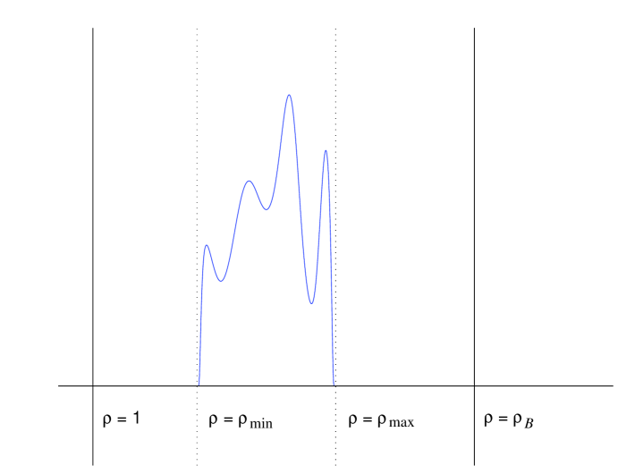
Figure 2. Initial wave–packet configuration in the frequency domain. The undulations represent the initial data which is compactly supported on $[\rho_{\mathrm{min}},\rho_{\mathrm{max}}]$. The domain $\mathsf{S}_{0}=(\rho_{\mathrm{max}},\infty)$ lies to the right of the data.

Let us now derive the explicit form of the radiation kernel, assuming that we now work in the region $\rho>\rho_{B}$. Consistent with our presentation thus far, we denote by $\psi_{l}(\tau,\rho)$ the function satisfying

(58) $${\mathcal{L}}[\psi_{l}](\sigma,\rho)=\hat{\psi}_{l}(\sigma,\rho)=a_{l}(\sigma)\rho^{-1}e^{-\sigma\rho_{*}}W_{l}(\sigma\rho;\sigma)\,.$$

Differentiation of this formula by $\rho$ then gives

(59) $$\partial_{\rho}\hat{\psi}_{l}(\sigma,\rho)=\left[\sigma\frac{W_{l}^{\prime}(\sigma\rho;\sigma)}{W_{l}(\sigma\rho;\sigma)}-\sigma-\frac{\sigma}{\rho-1}-\frac{1}{\rho}\right]\hat{\psi}_{l}(\sigma,\rho)\,,$$

with the prime denoting differentiation with respect to the first slot of $W_{l}(z;\sigma)$. Next, we rearrange terms and introduce some new symbols, thereby arriving at

(60) $$\frac{\sigma\hat{\psi}_{l}(\sigma,\rho)}{{\sf N}(\rho)}+\frac{\partial_{\rho}\hat{\psi}_{l}(\sigma,\rho)}{{\sf M}(\rho)}+\frac{\hat{\psi}_{l}(\sigma,\rho)}{{\sf M}(\rho)\rho}=\rho^{-1}{\sf N}(\rho)\hat{\psi}_{l}(\sigma,\rho)\left[\sigma\rho\,\frac{W_{l}^{\prime}(\sigma\rho;\sigma)}{W_{l}(\sigma\rho;\sigma)}\right]\,,$$

where in terms of the function $F(\rho)$ appearing in the line–element (14) we have introduced the temporal lapse function ${\sf N}(\rho)=F^{1/2}(\rho)$ and the radial lapse function ${\sf M}(\rho)=F^{-1/2}(\rho)$. The metrical function ${\sf N}$ describes the proper–time separation between neighboring three–dimensional level–$\tau$ hypersurfaces, whereas, in a given such three–surface, ${\sf M}$ describes the proper–radial separation between neighboring concentric two–spheres [27]. Upon inverse Laplace transformation, the last equation becomes

(61) $$\frac{1}{{\sf N}}\frac{\partial\psi_{l}}{\partial\tau}+\frac{1}{{\sf M}}\frac{\partial\psi_{l}}{\partial\rho}+\frac{\psi_{l}}{{\sf M}\rho}=\rho^{-1}{\sf N}(\rho)\psi_{l}(\tau,\rho)*{\mathcal{L}}^{-1}\left[\sigma\rho_{B}\,\frac{W_{l}^{\prime}(\sigma\rho_{B};\sigma)}{W_{l}(\sigma\rho_{B};\sigma)}\right](\tau)\,,$$

with $*$ here indicating Laplace convolution (defined just below). On this equation we remark that the direction ${\sf N}^{-1}\partial/\partial\tau+{\sf M}^{-1}\partial/\partial\rho$ is null and outgoing, whence the derivative of the field appearing on the lhs is along a characteristic. The last equation holds in particular at $\rho_{B}$, and as our robc we adopt the following:

(62) $$\left.\left[\frac{1}{{\sf N}}\frac{\partial\psi_{l}}{\partial\tau}+\frac{1}{{\sf M}}\frac{\partial\psi_{l}}{\partial\rho}+\frac{\psi_{l}}{{\sf M}\rho}\right]\right|_{\rho=\rho_{B}}=\rho_{B}^{-1}{\sf N}(\rho_{B})\int^{\tau}_{0}\omega_{l}(\tau-\tau^{\prime};\rho_{B})\psi_{l}(\tau^{\prime},\rho_{B}){\rm d}\tau^{\prime}\,,$$

where we have introduced the time–domain radiation kernel (tdrk)

(63) $$\omega_{l}(\tau;\rho_{B})={\mathcal{L}}^{-1}\left[\sigma\rho_{B}\,\frac{W_{l}^{\prime}(\sigma\rho_{B};\sigma)}{W_{l}(\sigma\rho_{B};\sigma)}\right](\tau)\,.$$

We refer to that appearing within the square brackets on the rhs as the frequency–domain radiation kernel (fdrk), and we also denote it by

(64) $$\hat{\omega}_{l}(\sigma;\rho_{B})=\sigma\rho_{B}\,\frac{W_{l}^{\prime}(\sigma\rho_{B};\sigma)}{W_{l}(\sigma\rho_{B};\sigma)}\,.$$

We assume that the fdrk $\hat{\omega}_{l}(\sigma;\rho_{B})$ has the appropriate $\sigma$–decay necessary for a well–defined $\omega_{l}(\tau;\rho_{B})={\mathcal{L}}^{-1}[\hat{\omega}_{l}(\sigma;\rho_{B})](\tau)$. Both $\omega_{l}(\tau;\rho_{B})$ and $\hat{\omega}_{l}(\sigma;\rho_{B})$ do of course depend on the values of $l$ and $\rho_{B}$ (and on the choice of spin $\jmath$), but to avoid clutter we will sometimes suppress this dependence and write simply $\omega(\tau)$ and $\hat{\omega}(\sigma)$. Finally, we note that the robc can be written simply as

(65) $$\left.\left[\frac{1}{{\sf N}}\frac{\partial\Psi_{l}}{\partial\tau}+\frac{1}{{\sf M}}\frac{\partial\Psi_{l}}{\partial\rho}\right]\right|_{\rho=\rho_{B}}=\rho_{B}^{-1}{\sf N}(\rho_{B})\int^{\tau}_{0}\omega_{l}(\tau-\tau^{\prime};\rho_{B})\Psi_{l}(\tau^{\prime},\rho_{B}){\rm d}\tau^{\prime}$$

in terms of the field $\Psi_{l}=\rho\psi_{l}$ appearing in (22).

1.4.2. Representation of the kernel

In Section 3 we undertake a fairly thorough numerical investigation of the analytic behavior of both $W_{l}(\sigma\rho_{B};\sigma)$ and $\hat{\omega}_{l}(\sigma;\rho_{B})$ as functions of the complex variable $\sigma$. As a result of our investigation, we shall make the following conjectures regarding the fdrk $\hat{\omega}_{l}(\sigma;\rho_{B})$. First, for $l$ fixed $\hat{\omega}_{l}(\sigma;\rho_{B})$ is analytic on ${\mathbb{C}}\backslash(-\infty,0]$, save for $N_{l}=N_{l}(\rho_{B})\in{\mathbb{Z}}_{\geq 0}$ simple poles with locations $\{\sigma_{l,n}=\sigma_{l,n}(\rho_{B}):n=1,\cdots,N_{l}\}$ lying in the lefthalf $\sigma$–plane. Second, $\hat{\omega}_{l}(\sigma;\rho_{B})$ is bounded in a neighborhood of the origin $\sigma=0$. Third, $\mathrm{Re}\hat{\omega}_{l}(\sigma;\rho_{B})$ is continuous and $\mathrm{Im}\hat{\omega}_{l}(\sigma;\rho_{B})$ jumps by a sign across the branch cut along the negative Re$\sigma$ axis. The integer $N_{l}(\rho_{B})$ is constant over sizable regions of the $\rho_{B}$ parameter space. However, the pole locations $\sigma_{l,n}$ do vary smoothly with respect to changes of $\rho_{B}$, apparently subject to

(66) $$\sigma_{l,n}(\rho_{B})\sim\sum_{k=1}^{\infty}\sigma_{l,n,k}\rho_{B}^{-k}\,,$$

where the $\sigma_{l,n,k}$ are constants. This series is perhaps only summable in the sense of an asymptotic expansion, and we have only numerically observed the first two terms.

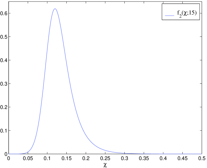
Figure 3. Typical cut profile. For this plot $l=2$, $\rho_{B}=15$, and $\jmath=0$.

Let us now define the $n$th pole strength and a cut profile respectively via the formulae

(67) $$\alpha_{l,n}(\rho_{B})=-\rho_{B}\sigma_{l,n}^{\prime}(\rho_{B})\,,\quad f_{l}(\chi;\rho_{B})=\mathrm{Im}\hat{\omega}_{l}(\chi e^{{\rm i}\pi};\rho_{B})\,,$$

with $\chi\geq 0$ and the prime here standing for $\partial/\partial\rho_{B}$ differentiation. Like the pole locations, both of these objects also vary with respect to changes of $\rho_{B}$ as indicated. As can be inferred from the third conjecture of the last paragraph, it is the case that $\mathrm{Im}\hat{\omega}_{l}(\chi e^{-{\rm i}\pi};\rho_{B})=-f_{l}(\chi;\rho_{B})$. To give a concrete example, we choose $\jmath=0$, $l=2$, and $\rho_{B}=15$, in which case we have numerically found that $N_{2}(15)=2$, $\sigma_{2,n}(15)\simeq-0.0969\pm{\rm i}0.0612$, and $\alpha_{2,n}(15)\simeq-0.0936\pm{\rm i}0.0647$, for $n=1(+)$ and $2(-)$. For these parameter values the corresponding cut profile is shown in Fig. 3. The plot is typical in the sense that for all $l$ and $\rho_{B}$ considered here, $f_{l}(\chi;\rho_{B})$ decays sharply in the $\chi\rightarrow 0^{+}$ and $\chi\rightarrow\infty$ limits (except for $l=0$ where the decay in the $\chi\rightarrow 0^{+}$ limit is not as sharp). However, the shape of the profile can be qualitatively different for other parameter values. Moreover, for certain exceptional values of the parameters, the profile can even blow up at a particular $\chi$ point, in which case numerical evidence suggests that the integral in (68) is defined in the sense of a Cauchy Principal Value. We discuss all of these issues in Section 3.1.

In terms of the pole locations and strengths and the cut profile, we claim that the fdrk has the following representation (suppressing $\rho_{B}$ dependence for now):

(68) $$\hat{\omega}_{l}(\sigma)=\sum_{n=1}^{N_{l}}\frac{\alpha_{l,n}}{\sigma-\sigma_{l,n}}-\frac{1}{\pi}\int^{\infty}_{0}\frac{f_{l}(\chi)}{\sigma+\chi}\,{\rm d}\chi\,,$$

for all $\sigma$ not equal to a $\sigma_{l,n}$ and not lying on $(-\infty,0]$. Despite the right closed bracket here, we shall also evaluate this representation at $\sigma=0$. Given the described structure of the $\sigma$–function $\hat{\omega}_{l}(\sigma)$, the derivation of such a representation amounts to a simple exercise involving the Residue Theorem and a “keyhole” contour. Although we will often describe the second term on the rhs of (68) as corresponding to a continuous set of poles, these are not really poles in the sense of complex analysis (which are properly isolated singularities). Formally, we compute the inverse Laplace transform of (68), with result

(69) $$\omega_{l}(\tau)=\sum_{n=1}^{N_{l}}\alpha_{l,n}\exp(\sigma_{l,n}\tau)-\frac{1}{\pi}\int^{\infty}_{0}f_{l}(\chi)\exp(-\chi\tau){\rm d}\chi\,.$$

Evidently then, direct numerical construction of the fdrk would amount to numerical computation of the pole locations and strengths and the cut profile. For $l\leq 10$ we consider such a direct construction in Section 3.2, although we show in Section 3.3 how this brute–force approach may be bypassed insofar as implementation of robc is concerned.

1.4.3. Comparison with the Green’s function method

Any temptation to identify the pole locations $\sigma_{l,n}(\rho_{B})$ in the representation (68) with so–called quasinormal modes [68] should be resisted. For a given $l$ there are an infinite number of quasinormal modes [68], fixed numerical values intrinsic to the blackhole geometry and certainly insensitive to any particular choice of outer boundary radius $\rho_{B}$. However, for $\rho_{B}>1$ the poles now under examination, that is the zeros in $\sigma$ of the Heun–type function $W_{l}(\sigma\rho_{B};\sigma)$, are finite in number, and they do depend on $\rho_{B}$. Moreover, the boundary value problem associated with these Heun zeros is different than the usual one associated with quasinormal modes. This usual boundary value problem was considered in the pioneering work [38] of Leaver, and more recently in a careful study by Andersson [39]. The goal of both authors was to examine a given multipole field $\psi_{l}(\tau,\rho)=\rho^{-1}\Psi_{l}(\tau,\rho)$ in terms of a Green’s function representation involving initial data. Andersson refers to this as the initial value problem for the scalar field (or, more generally, for electromagnetic or gravitational perturbations), although when we mentioned that name in the first paragraph of the introduction we did not have this Green’s function approach in mind. In Eq. (6) of [39], Andersson expresses the scalar field as

(70) $$\Psi_{l}(\tau,\rho_{*})=\int G_{l}(\rho_{*},\rho_{*}^{\prime};\tau)\partial_{\tau}\Psi_{l}(0,\rho_{*}){\rm d}\rho_{*}^{\prime}+\int\partial_{\tau}G_{l}(\rho_{*},\rho_{*}^{\prime};\tau)\Psi_{l}(0,\rho_{*}){\rm d}\rho_{*}^{\prime}\,.$$

In this equation we view the field $\Psi_{l}$ introduced in (44) as depending on $\rho_{*}$ (as Andersson does), and we have also slightly modified Andersson’s notations to suit our own. The appropriate limits of $\rho_{*}$ integration in (70) are discussed in [39]. This problem perhaps resembles our own; however, as we now demonstrate, it is different both in concept and detail.

Both Leaver and Andersson considered the (here Laplace) transform of the Green’s function in (70), a frequency–domain Green’s function $\hat{G}_{l}(\rho_{*},\rho_{*}^{\prime};\sigma)$ associated with the following boundary value problem. The solution is pure ingoing at the horizon [$\hat{\Psi}^{-}_{l}(\sigma,\rho_{*})\sim\exp(\sigma\rho_{*})$ as $\rho_{*}\rightarrow-\infty$] and outgoing at infinity [$\hat{\Psi}^{+}_{l}(\sigma,\rho_{*})\sim\exp(-\sigma\rho_{*})$ as $\rho_{*}\rightarrow\infty$]. In fact, we briefly considered $\hat{G}_{l}(\rho_{*},\rho_{*}^{\prime};\sigma)$ in and around (57), although we shall make no further use of it in this article or the follow–up article. Leaver and Andersson’s approach was essentially to examine the value $\Psi_{l}(\tau,\rho_{*})$, as expressed by (70), via a careful analysis of $\hat{G}_{l}(\rho_{*},\rho_{*}^{\prime};\sigma)$. (Of no concern here, Leaver further considered more general driving source terms beyond just the initial data.) When $\hat{G}_{l}(\rho_{*},\rho_{*}^{\prime};\sigma)$ is considered as an analytic function of complex $\sigma$ and continued into the lefthalf plane, its pole locations are the quasinormal modes and there is also an associated branch cut along the negative Re$\sigma$ axis [38, 39, 65]. These complex analytic features play a prominent role in describing the physical behavior of the field (see [38, 39] and references therein).

Our key representation (68) stems from continuation into the lefthalf $\sigma$–plane of the fdrk $\hat{\omega}_{l}(\sigma;\rho_{B})$, the expression (64) involving the logarithmic derivative of $W_{l}(\sigma\rho;\sigma)=\exp(\sigma\rho_{*})\hat{\Psi}^{+}_{l}(\sigma,\rho)$. Here we again view $\hat{\Psi}_{l}$ as depending on $\rho$, rather than $\rho_{*}$ as in the last paragraph. We stress that the fdrk $\hat{\omega}_{l}(\sigma;\rho_{B})$ is not the Green’s function $\hat{G}_{l}(\rho_{*},\rho_{*}^{\prime};\sigma)$ considered by both Leaver and Andersson. Indeed, $\hat{\omega}_{l}(\sigma;\rho_{B})$ is a boundary integral kernel. Moreover, it is built solely with the outgoing solution $\hat{\Psi}^{+}_{l}$ to the homogeneous ode, whereas construction of the Green’s function requires two linearly independent homogeneous solutions, $\hat{\Psi}^{-}_{l}$ and $\hat{\Psi}^{+}_{l}$. As mentioned, the pole locations associated with $\hat{\omega}_{l}(\sigma;\rho_{B})$ are not the quasinormal modes, rather the special frequencies, finite in number, for which the outgoing solution $W_{l}(\sigma\rho;\sigma)$ also vanishes at $\rho_{B}$. Despite the fact that $\hat{G}_{l}(\rho_{*},\rho_{*}^{\prime};\sigma)$ and $\hat{\omega}_{l}(\sigma;\rho_{B})$ are different integral kernels, we remark that they share the same qualitative features in the lefthalf $\sigma$–plane (each has poles and a branch cut).

On top of these technical differences between our work and those of Leaver and Andersson, we point out that our overall goal is very different. As mentioned, their goal was to examine the actual value of the field via the representation (70) based on spatial convolution. On the contrary, our boundary kernel $\omega_{l}(\tau;\rho_{B})$ is associated with temporal convolution, with the goal being to impose exact radiation boundary conditions at a given outer sphere $B$. That is to say, our goal is domain reduction via the introduction of integral convolution over the history ${}^{3}\!B$ of the boundary $B$. With this distinction in mind, compare our key Eq. (62) with Andersson’s key equation, as we have written it in (70). Perhaps the approach of Andersson and Leaver could also be used to numerically implement exact radiation boundary conditions in an alternative way [by setting $\rho_{*}=\rho_{B}+\log(\rho_{B}-1)$ in (70)], but they did not address this question per se. Moreover, such an approach would necessarily relate robc to the details of the data on the initial surface, which would seem awkward from a numerical standpoint. Even were such an implementation carried out, memory and speed issues would inevitably arise. Besides developing exact robc via domain reduction, we also intend to provide an efficient and rapid implementation of these conditions.

1.4.4. Approximation of the kernel

Our numerical implementation of robc rests on approximation of the exact kernel $\omega(\tau)$ (now suppressing $l$ as well as $\rho_{B}$) by a compressed kernel $\xi(\tau)$. We explain this terminology later, but here collect an estimate needed to address the relative error associated with such an approximation. We start with the Laplace inversion formula,

(71) $$\psi(\tau)=\frac{1}{2\pi{\rm i}}\int^{{\rm i}\infty}_{-{\rm i}\infty}\hat{\psi}(\sigma)e^{\sigma\tau}{\rm d}\sigma\,,$$

where we are assuming that any singularities of $\hat{\psi}(\sigma)$ lie in the lefthalf plane Re$\sigma<0$. A change of variables casts the inversion formula into the form

(72) $$\psi(\tau)=\frac{1}{2\pi}\int^{\infty}_{-\infty}\hat{\psi}({\rm i}y)e^{{\rm i}y\tau}{\rm d}y\,,$$

thereby introducing the Fourier transform $\widetilde{\psi}(y)=\hat{\psi}({\rm i}y)$ of $\psi(\tau)$. It then follows that

(73) $$\big{\|}\psi\big{\|}_{L_{2}(0,\infty)}=\big{\|}\psi\big{\|}_{L_{2}(\mathbb{R})}=\big{\|}\widetilde{\psi}\big{\|}_{L_{2}(\mathbb{R})}\,.$$

The first equality follows subject to the assumption that $\psi(\tau)$ vanishes for $\tau\leq 0$, while the second is Parseval’s identity.

Now suppose $\xi(\tau)$, with Fourier transform $\widetilde{\xi}(y)$, is an approximation to the kernel $\omega(\tau)$. Later we shall have its Laplace transform $\hat{\xi}(\sigma)$ as a rational function $P(\sigma)/Q(\sigma)$, and then $\widetilde{\xi}(y)=P({\rm i}y)/Q({\rm i}y)$. Also introduce the Fourier transform $\widetilde{\omega}(y)=\hat{\omega}({\rm i}y)$ of $\omega(\tau)$. In terms of these variables we have

(74) $$\big{\|}\xi*\psi-\omega*\psi\big{\|}_{L_{2}(0,\infty)} =\big{\|}\widetilde{\xi}\widetilde{\psi}-\widetilde{\omega}\widetilde{\psi}\big{\|}_{L_{2}(\mathbb{R})}$$

$$\leq{\rm sup}_{y\in\mathbb{R}}\frac{|\widetilde{\xi}(y)-\widetilde{\omega}(y)|}{|\widetilde{\omega}(y)|}\times\big{\|}\widetilde{\omega}\widetilde{\psi}\big{\|}_{L_{2}(\mathbb{R})}$$

$$={\rm sup}_{\sigma\in{\rm i}\mathbb{R}}\frac{|\hat{\xi}(\sigma)-\hat{\omega}(\sigma)|}{|\hat{\omega}(\sigma)|}\times\big{\|}\omega*\psi\big{\|}_{L_{2}(0,\infty)}$$

as our basic estimate. Because of this estimate, we focus on finding approximations $\hat{\xi}(\sigma)$ to $\hat{\omega}(\sigma)$ which have small relative supremum error along the imaginary axis.

Finally, suppose that we do not quite know $\hat{\omega}({\rm i}y)$. Rather, as is the case, we must generate $\hat{\omega}({\rm i}y)$ itself numerically. Then, instead of the relative error

(75) $${\rm sup}_{\sigma\in{\rm i}\mathbb{R}}\frac{|\hat{\xi}(\sigma)-\hat{\omega}(\sigma)|}{|\hat{\omega}(\sigma)|}\,,$$

we should consider an expression like

(76) $${\rm sup}_{\sigma\in{\rm i}\mathbb{R}}\frac{|\hat{\xi}(\sigma)-\hat{\omega}(\sigma)|}{|\hat{\omega}(\sigma)|}+{\rm sup}_{\sigma\in{\rm i}\mathbb{R}}\frac{|\Delta\hat{\omega}(\sigma)|}{|\hat{\omega}(\sigma)|}\,,$$

where the final term is an estimate of the supremum relative error in our knowledge of $\hat{\omega}({\rm i}y)$. For the methods we develop to generate $\hat{\omega}({\rm i}y)$, this second term is negligible with respect to the first one.

2. Numerical evaluation of the outgoing solution and kernel

This section describes the handful of numerical methods used in this work. The first subsection describes a numerical method for evaluating the outgoing solution $W_{l}(\sigma\rho_{B};\sigma)$ at a given complex $\sigma$, and this method allows us to numerically study the analytic structure of $W_{l}(\sigma\rho_{B};\sigma)$ as a function of Laplace frequency. The lefthalf $\sigma$–plane is the domain of interest, and a study of $W_{l}(\sigma\rho_{B};\sigma)$ on this domain, carried out in Section 3.1, justifies the key representation (68). As we indicated in Section 1.4.4, our numerical approximations to the fdrk $\hat{\omega}_{l}(\sigma;\rho_{B})$ are tailored to have small relative supremum error along the Im$\sigma$ axis. Therefore, insofar as implementation of robc is concerned, we primarily need numerical methods for obtaining accurate numerical profiles for Re$\hat{\omega}_{l}({\rm i}y;\rho_{B})$ and Im$\hat{\omega}_{l}({\rm i}y;\rho_{B})$ with $y\in\mathbb{R}$. The second subsection describes two such methods.

Before describing our numerical methods, we note that Leaver has analytically represented a solution to the Regge–Wheeler equation (more generally to the generalized spheroidal wave equation) as an infinite series in Coulomb wave functions, where the expansion coefficients obey a three–term recursion relation [44]. Such a series can alternatively be viewed as a sum of confluent hypergeometric functions. One approach towards our goal of numerically evaluating the outgoing solution would be to use the appropriate Leaver series. However, beyond the issue of numerically solving the relevant three–term recursion relation, numerical evaluation of Coloumb wave functions (for complex arguments) is already somewhat tricky [60]. Here we describe far simpler methods, which are nevertheless extremely accurate. Although simple, our methods are very accurate only for a limited range of frequencies (which happen to be precisely the frequencies we are interested in). The Leaver series is valid over the whole frequency plane. Although we have not compared our methods with the Leaver series, we believe they are better suited for our purposes.

2.1. Numerical evaluation of the outgoing solution

From now on let us simply refer to $W_{l}(\sigma\rho_{B};\sigma)$ as a Heun function and $W_{l}(\sigma\rho_{B})$ as a Bessel function. This is not quite correct since, as discussed in Section 1.3.2, $W_{l}(\sigma\rho_{B};\sigma)$ and $W_{l}(\sigma\rho_{B})$ respectively differ from Heun and Bessel functions by transformations on the dependent variable; however, this terminology will streamline our presentation. We now present numerical methods for computing the complex value $W_{l}(\sigma\rho_{B};\sigma)$. The methods have been designed to successfully compute the similar value $W_{l}(\sigma\rho_{B})$, formally $W_{l}(\sigma\rho_{\rm B};0)$ in our notation. $W_{l}(\sigma\rho)$ solves the ode

(77) $$\frac{\mathrm{d}^{2}\hat{\Phi}_{l}}{\mathrm{d}\rho^{2}}-2\sigma\frac{\mathrm{d}\hat{\Phi}}{\mathrm{d}\rho}-\frac{l(l+1)}{\rho^{2}}\hat{\Phi}=0$$

obtained directly from (46) via the substitution $z=\sigma\rho$. Section 1.3.3 noted that $W_{l}(\sigma\rho)$ is a polynomial $\sum_{n=0}^{l}c_{n}(\sigma\rho)^{-n}$ of degree $l$ in inverse $\sigma\rho$, with coefficients $c_{n}$ given in (52). With the exact form of $W_{l}(\sigma\rho)$ we could in principle compute the value $W_{l}(\sigma\rho_{B})$ directly. Nevertheless, if we pretend that the exact form of $W_{l}(\sigma\rho)$ is not at our disposal, then the task of numerically computing $W_{l}(\sigma\rho_{B})$ shares essential features with our ultimate task of computing $W_{l}(\sigma\rho_{B};\sigma)$. The task of computing $W_{l}(\sigma\rho_{B})$ has been an invaluable model, and for ease of presentation we mostly focus on it here.

2.1.1. Numerical integration

Focusing on the $\rho$–dependence of the solution, we write $W_{l}(\sigma\rho)=\sum_{n=0}^{l}(c_{n}\sigma^{-n})\rho^{-n}$. Since we shall not allow ourselves to evaluate $W_{l}(\sigma\rho_{B})$ as $\sum_{n=0}^{l}(c_{n}\sigma^{-n})\rho^{-n}_{B}$, we truncate the series after some fixed number $l-p$ of terms, assuming that

(78) $$W_{l}(\sigma\rho)\sim\sum_{n=0}^{l-p}(c_{n}\sigma^{-n})\rho^{-n}$$

is at our disposal. Truncation by hand of this already finite series serves as a model for the scenario involving $W_{l}(\sigma\rho;\sigma)$, where only a divergent formal series, such as the one specified by (49) and (50), is at our disposal. With our truncated series we can still generate an accurate approximation to the value $W_{l}(\sigma\rho_{\infty})$, so long as $\rho_{\infty}$ is large enough. Let us set $\rho_{\infty}={\tt scale}*\rho_{B}$, with ${\tt scale}$ a large number. Evaluation of the truncated sum and its $\rho$ derivative at $\rho_{\infty}$ then generates initial data for the ode. Moreover, the generated data is approximate to the exact data $\{W_{l}(\sigma\rho_{\infty}),W^{\rho}_{l}(\sigma\rho_{\infty})\}$ giving rise to $W_{l}(\sigma\rho)$. Here the superscript $\rho$ denotes $\partial/\partial\rho$ differentiation, whereas a prime ^′ would denote differentiation in argument. We stress that our approximation to the exact data can be rendered arbitrarily accurate by choosing $\rho_{\infty}$ large enough. Finally, we numerically integrate (77) in $\rho$ from $\rho_{\infty}$ all the way down to $\rho_{B}$, thereby computing a candidate for the value $W_{l}(\sigma\rho_{B})$.

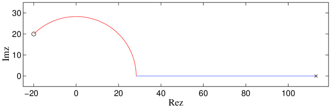
Figure 4. Two–component path in $z$–plane. The figure depicts the ray–and–arc path described in the text. Here we have $\rho_{B}=20$, $\sigma=-1+{\rm i}$, and ${\tt scale}=4$, so that $z_{B}=-20+{\rm i}20$ (marked by an o) and $z_{\infty}=4*20*\sqrt{2}\simeq 113$ (marked by an x). Typically scale will be much larger, but the value here makes for a good figure.

As it stands, the description in the last paragraph is an outline for a stable numerical method, provided Re$\sigma>0$. However, for the case Re$\sigma<0$ of interest the described method is not stable. To see why, consider the $l=1$ outgoing solution $W_{1}(\sigma\rho)=1+(\sigma\rho)^{-1}$ to (77). As a second linearly independent solution to the $l=1$ ode, take the ingoing solution $Z_{1}(\sigma\rho)=\exp(2\sigma\rho)[1-(\sigma\rho)^{-1}]$. Further, suppose that initial data for the ode is obtained from a truncated sum as described above, with $\{1,0\}$ in place of exact data $\{1+(\sigma\rho_{\infty})^{-1},-\sigma(\sigma\rho_{\infty})^{-2}\}$. The initial data $\{1,0\}$ corresponds to a linear combination $aW_{1}(\sigma\rho)+bZ_{1}(\sigma\rho)$ with $a\simeq 1$ and $b$ such that $bZ_{1}(\sigma\rho_{\infty})\simeq 0$. To fix some realistic numbers, let $\rho_{B}=20$, ${\tt scale}=250$ so $\rho_{\infty}=5000$, and $\sigma=-0.05$. Then we compute $a\simeq 1.0040$ and $bZ_{1}(\sigma\rho_{\infty})\simeq 8.0320\times 10^{-6}$, where $b\simeq 1.1229\times 10^{212}$. The exact value we wish to calculate is $W_{1}(-1)=0$. However, with the chosen initial data, even an exact integration of (77) from $\rho_{\infty}=5000$ to $\rho_{B}=20$ yields the value $3.0393\times 10^{211}$. Since error in the initial conditions is exponentially enhanced, the second solution $Z_{1}(-0.05\rho)$ becomes dominant as $\rho$ is decreased.

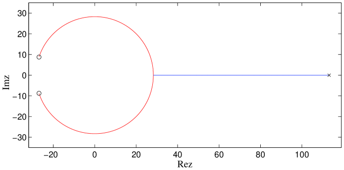
Figure 5. Mirror image paths. The figure depicts the two globally different paths connecting $z_{\infty}$ to $z$–points above and below the negative Re$z$ axis. Use of such different paths puts a branch cut on the negative Re$z$ axis for Heun functions and for Bessel functions not of half–integer order.

2.1.2. Two–component path integration

The simple discussion at hand suggests that we should complexify the variable $\rho$, rotating $\rho_{\infty}$ off the real axis by an angle $\theta$ large enough to ensure that the product $\sigma\rho_{\infty}$ lies in the righthalf plane. Then integration along a ray in the complex $\rho$–plane from $\rho_{\infty}$ towards the complex point $\exp({\rm i}\theta)\rho_{B}$ (with $\rho_{B}$ still real here) would exponentially suppress error in the initial conditions. At the end of such a ray integration, a second integration over an arc of $\theta$ radians would be needed to undo the phase of $\exp({\rm i}\theta)\rho_{B}$. We effect such a rotation of the $\rho$ coordinate as follows. We choose to work with the variable $z=\sigma\rho$, the solution $W_{l}(z)$, and the truncated series $\sum_{n=0}^{l-p}c_{n}z^{-n}$. Our integration will now be carried out in the complex $z$–plane rather than the $\rho$–plane, although the strategy is essentially the same. We define $z_{\infty}$ to be a large real number ${\tt scale}*|\sigma\rho_{B}|$, and obtain initial data approximate to $\{W_{l}(z_{\infty}),W_{l}^{\prime}(z_{\infty})\}$ via evaluation of the truncated series and its $z$ derivative at $z_{\infty}$. Even for large $l$ we have typically chosen $l-p=5$ terms to define the truncated series. Then to compute $W_{l}(\sigma\rho_{B})$, we must numerically integrate the ode (46) from $z_{\infty}$ to $z_{B}=\sigma\rho_{B}$ along some path in the complex $z$–plane. A possible two–component path is shown in Fig. 4. It is composed of a straight ray followed by a circular arc, with the terminal point of the ray being the real $z$–point $|\sigma\rho_{B}|$. The arc subtends an angle equal to the argument of $\sigma$. If $\sigma$ happens to lie in the third quadrant, then the relevant two–component path looks like the one in Fig. 4 except reflected across the Re$z$ axis.

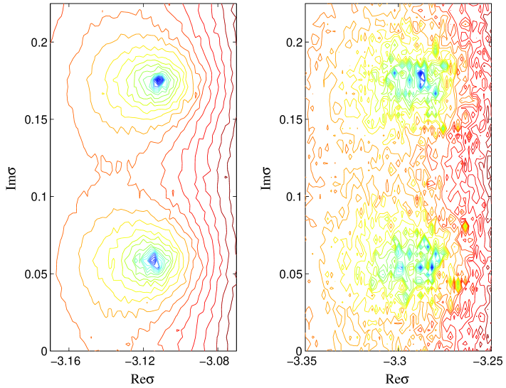
Figure 6. Contour lines of $\log|W_{l}(15\sigma)|$ on $\sigma$–plane for $l=70$ and $74$. On the lhs we plot $\log|W_{70}(15\sigma)|$. The method used to generate this plot is the one based on two–component paths, and the integration scheme along each path component is fifth–order Runga–Kutta–Fehlberg [62]. Relevant parameters here are $I=50$, $J=50$, $N=49152$, $M=49152$, $l=70$, $\rho_{B}=15$, ${\tt scale}=500$, $p=65$, and $\kappa=1$. $I$ and $J$ respectively specify the vertical and horizontal discretization of the $\sigma$–plane. $N$ and $M$ are respectively the number of integration steps along the ray and arc. Other parameters are described in the text. On the rhs $l=74$ rather than $70$ and $p=69$ rather than $65$ (the initial condition is still determined by $5=l-p$ terms). All other parameters are the same as for the lhs plot.

Evaluation of the Heun function $W_{l}(\sigma\rho_{B};\sigma)$ features numerical integration of the ode (44) from $z_{\infty}$ to $z_{B}=\sigma\rho_{B}$ along the same two–component path. Although $z$ of course changes along the integration path, the $\sigma$ in $W_{l}(z;\sigma)$ remains fixed throughout the integration. We are then integrating a different ode for each value of $\sigma$. Since these Heun functions are not bispectral (see the discussion in Section 1.2.3), there would seem no way around such a cumbersome approach. Were we only interested in $W_{l}(\sigma\rho_{B})$, and not $W_{l}(\sigma\rho_{B};\sigma)$ as well, such an approach would be unnecessary (for then we could integrate with respect to frequency $\sigma$). In essence our two–component path method for evaluation of either $W_{l}(\sigma\rho_{B})$ or $W_{l}(\sigma\rho_{B};\sigma)$ is an integration with respect to radius rather than frequency. Indeed, even for the Bessel case, we connect each $z_{B}$ to the point $z_{\infty}$ by its own integration path, and during the integration do not record values for $W_{l}(z)$ along the path. Recording such values throughout the integration would be a more efficient way of mapping out the $\sigma$ dependence of $W_{l}(\sigma\rho_{B})$.

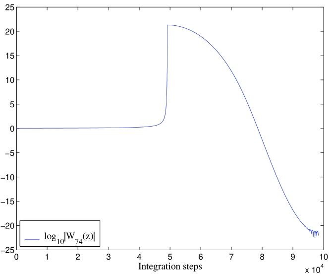
Figure 7. Value of $\log_{10}|W_{74}(z)|$ along two–component path from $z_{\infty}$ to $z_{B}=15\sigma$ for $\sigma=-3.29128+{\rm i}0.05785$. The point $-3.29128+{\rm i}0.05785$ is close to a zero of $W_{74}(15\sigma)$ and lies in the region of the $\sigma$–plane shown in Fig. 6. The parameters here are the same as those listed in the caption of Fig. 6. Along the horizontal axis we have the $N+M=98304$ integration steps. The function is of order unity at $z_{\infty}$ and close to zero at the terminal point $z_{B}$. However, note that the modulus of $W_{74}(z)$ gets larger than $10^{20}$ during the integration.

Let us note two key features of two–component paths. First, for any choice of $z_{B}\neq 0$ the associated path avoids the origin where the function $W_{l}(z)$ is singular. Second, considering two terminal points, one $z^{\mathsf{a}}_{B}$ just above and the other $z^{\mathsf{b}}_{B}$ just below the negative real axis, we note that the respective two–component paths connecting them to $z_{\infty}$ are mirror images, as depicted in Fig. 5. Therefore, the path leading from $z_{\infty}$ to $z^{\mathsf{a}}_{B}$ is globally different than the path leading from $z_{\infty}$ to $z^{\mathsf{b}}_{B}$, this being true despite the fact that $z^{\mathsf{a}}_{B}$ and $z^{\mathsf{b}}_{B}$ may lie arbitrarily close to each other in the $z$–plane. For $l\in\mathbb{Z}_{\geq 0}$ the functions $W_{l}(z)$ are clearly analytic on the punctured $z$–plane, so that $W_{l}(z^{\mathsf{a}}_{B})=W_{l}(z^{\mathsf{b}}_{B})$ in the limit that these points meet on the negative Re$z$ axis. However, for Heun functions we shall find $W_{l}(z^{\mathsf{a}}_{B};\sigma^{\mathsf{a}})\neq W_{l}(z^{\mathsf{b}}_{B};\sigma^{\mathsf{b}})$, and in turn $W_{l}(\sigma^{\mathsf{a}}\rho_{B};\sigma^{\mathsf{a}})\neq W_{l}(\sigma^{\mathsf{b}}\rho_{B};\sigma^{\mathsf{b}})$, for corresponding $\sigma^{\mathsf{a}}=z_{B}^{\mathsf{a}}/\rho_{B}$ and $\sigma^{\mathsf{b}}=z_{B}^{\mathsf{b}}/\rho_{B}$. Therefore, the negative Re$\sigma$ axis is a branch cut for $W_{l}(\sigma\rho_{B};\sigma)$ as a function of $\sigma$. Our path choices for connecting points in the second and third quadrants to $z_{\infty}$ have been made precisely to put this branch cut on the negative Re$\sigma$ axis.

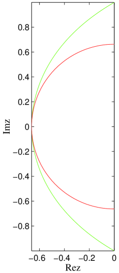
Figure 8. Asymptotic curve $\mathcal{C}$. The large curve $\mathcal{C}$ is the one described in the text and near which the scaled zeros of the MacDonald function lie. It has parametric form $z(\lambda)=-\sqrt{\lambda^{2}-\lambda\tanh\lambda}\pm{\rm i}\sqrt{\lambda\coth\lambda-\lambda^{2}}$ for $\lambda$ in the domain $[0,\lambda_{0}]$ with $\lambda_{0}\simeq 1.1997$ such that $\tanh\lambda_{0}=1/\lambda_{0}$. The small curve is a circle tangent to the $\mathcal{C}$ point $(x_{0},0)$, where $x_{0}=-\sqrt{\lambda_{0}^{2}-1}\simeq-0.6627$.

As we demonstrate below, the described two–component path method is quite accurate for low $l$. However, for large $l$ and some values of $\sigma$ there is a considerable loss of precision associated with evaluating $W_{l}(\sigma\rho_{B})$ by this method (this is true no matter what integration scheme is used along the path components). Therefore, we shortly introduce a more accurate method based on one–component paths. Before turning to the improved method, let us first heuristically describe the trouble the two–component method can run into for large $l$. In Fig. 6 we graphically demonstrate the breakdown in the method which occurs (for the specified parameter values) when $l$ gets beyond $70$. The relevant task under consideration is to obtain $W_{l}(\sigma\rho_{B})$ in a region around those zeros of $W_{l}(\sigma\rho_{B})$ which have large negative real parts. On the lhs we plot $\log|W_{70}(15\sigma)|$, using the logarithm to distribute contour lines more evenly. For the portion of the $\sigma$–plane shown only two of seventy zero locations are evident. Note the onset of degradation in the numerical solution. On the rhs we plot $\log|W_{74}(15\sigma)|$, and in the plot two of seventy–four zero locations are somewhat evident, despite significant degradation. This degradation stems from the following phenomenon. Although they do avoid the origin, two–component integration paths, especially those which terminate near a zero with large negative real part, tend to pass through a region near the origin where the solution is quite large. The phenomenon becomes more pronounced as $l$ grows. Two–component paths connect $z_{\infty}$ (where the solution is of order unity) to $z_{B}$ (which might be at or near a zero of the solution in question), and at each of these points the solution is in some sense small. Therefore, loss of accuracy is an issue if the connecting path indeed passes through a large–solution region. We document an instance of this situation in Fig. 7.

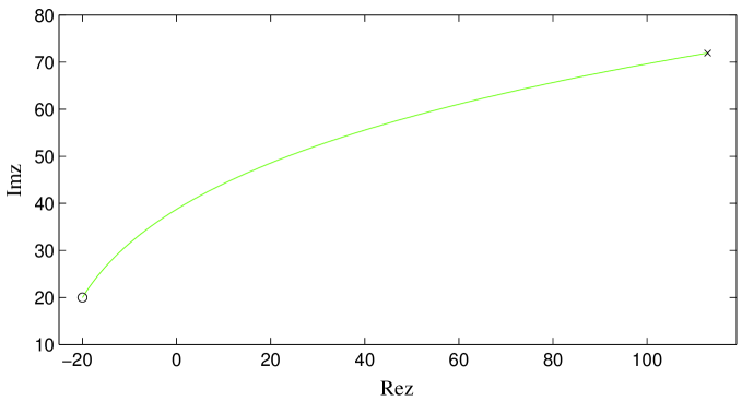
Figure 9. One–component path. To generate the depicted curve we have set $R\simeq 38.7479$ and chosen $\eta$ from the range $0.5162\lesssim\eta\lesssim 1.8650$, ensuring that the terminal point $z_{B}=20+{\rm i}20$ and the initial point $z_{\infty}\simeq 113+{\rm i}72$ (comparable with the analogous point in Fig. 4). For one–component paths the meaning of the scale variable is a little different. For such paths the real component of $z_{\infty}$ is set by $R*{\tt scale}$.

2.1.3. One–component path integration

We now describe an alternative class of integration paths tailored to mitigate the problem of passing through regions where the solution is large. Members of this alternative class are one–component paths, and this new class yields an improved version of the integration method based the two–component paths. As the new method will be more accurate, we will use it to quantify the accuracy of the two–component method.

The one–component paths of interest are essentially dilations of a certain curve $\mathcal{C}$ depicted in Fig. 8. A parametric description of $\mathcal{C}$ in terms of transcendental functions is given in the figure caption. The curve $\mathcal{C}$ is intimately related to the zeros of $W_{l}(z)$, also the zeros of the MacDonald function $K_{l+1/2}(z)$. As a degree–$l$ polynomial in inverse $z$, the function $W_{l}(z)$ has $l$ zeros. Let $n\in\mathbb{Z}_{\geq 0}$ run from $1$ to $l$ (with $n=0$ if $l=0$) and $k_{l,n}$ denote the zeros of $W_{l}(z)$. It is known that the scaled zeros $(l+1/2)^{-1}k_{l,n}$ lie arbitrarily close to $\mathcal{C}$ as $l$ becomes large (see results listed or summarized in Refs. [61, 18, 63, 21]). A simple numerical experiment performed in Section 3.1.1 confirms this assertion even for small $l$. Therefore, for a given $l$, dilation of $\mathcal{C}$ by $l+1/2$ yields a curve on which the solution $W_{l}(z)$ tends to remain small. Our one–component integration paths are quartic approximations to (dilations of) $\mathcal{C}$, and an example is depicted in Fig. 9. The approximation is given parametrically by $R(g(\eta),\eta)$, where $R$ is fixed and $g(\eta)=a\eta^{4}+b\eta^{2}+c$ is a quartic polynomial such that upon multiplication by $R$ the $\mathcal{C}$ points $(0,\pm 1)$, $(x_{1},\pm y_{1})$, and $(x_{0},0)$ all lie on the parametric approximation. We have $x_{1}=-\sqrt{2/(e^{2}+1)}$, $y_{1}=\sqrt{2/(e^{2}-1)}$, and $x_{0}=-\sqrt{\lambda_{0}^{2}-1}$ with $\lambda_{0}\simeq 1.1997$ obeying $\tanh(\lambda_{0})=1/\lambda_{0}$. From the parametric description of $\mathcal{C}$ given in the caption of Fig. 8, one may verify that each of these points indeed lies on $\mathcal{C}$. Numerically then $a\simeq 0.1534$, $b\simeq 0.5093$, and $c\simeq-0.6627$.

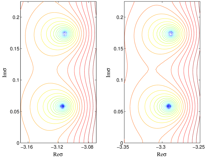
Figure 10. Contour lines of $\log|W_{l}(15\sigma)|$ on $\sigma$–plane for $l=70$ and $74$. On the lhs we have plotted $\log|W_{70}(15\sigma)|$. The method used to generate the plot is the one based on the one–component paths, again with Runga–Kutta–Fehlberg integration. Relevant parameters here are $I=50$, $J=50$, $P=98304$, $l=70$, $\rho_{B}=15$, ${\tt scale}=500$, $p=65$, and $\kappa=1$. $P$ is the number of subintervals for the numerical integration. Other parameters are described in the text or the caption for Fig. 6. The plot on the rhs is nearly the same, except that now $l=74$ and $p=69$ (i.e. the initial condition still determined by $5=l-p$ terms). All other parameters are the same as for the lhs plot.

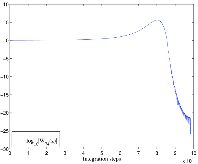
Figure 11. Value of $\log_{10}|W_{74}(z)|$ along one–component path from $z_{\infty}$ to $z_{B}=15\sigma$ for $\sigma=-3.29128+{\rm i}0.05785$. The point $-3.29128+{\rm i}0.05785$ is close to a zero of $W_{74}(15\sigma)$ and lies in the region of the $\sigma$–plane shown in Fig. 10. Along the horizontal axis we have the $P=98304$ integration steps. Note that the modulus of $W_{74}(z)$ never gets so large as it does in Fig. 7.

We repeat the graphical investigation described and carried out at the end of Section 2.1.2, but now with the one–component method. The relevant contour plots of $\log|W_{70}(15\sigma)|$ and $\log|W_{74}(15\sigma)|$ are shown in Fig. 10. Comparing this set of plots with the corresponding set in Fig. 6, we see significantly less degradation in former set. Moreover, we again investigate the size of the solution along an integration path in Fig. 11. These figures and their captions argue that the method based on one–component paths is more accurate than the one based on two–component paths, at least insofar as zero–finding is concerned.

2.1.4. Accuracy of the numerical evaluation

To check the accuracy of our methods for evaluating either $W_{l}(\sigma\rho_{B};\sigma)$ or $W_{l}(\sigma\rho_{B})$ we may compare values obtained independently from one–component path and two–component path integration. For the evaluation of $W_{l}(\sigma\rho_{B})$ there are other checks. First, numerical values for $W_{l}(\sigma\rho_{B})$ can be checked against direct evaluations of $\sum_{n=0}^{l}c_{n}(\sigma\rho_{B})^{-n}$. However, as we have seen in (54), for large $l$ the final coefficient $c_{l}$ and the ones just before it quickly become too large to faithfully evaluate this exact expression. One can use extended precision (say in Mathematica) to get around this problem. Another check, useful for large values of $l$ even without extended precision, involves the known continued fraction expansion

(79) $$z\frac{W_{l}^{\prime}(z)}{W_{l}(z)}=-\frac{l(l+1)}{2(z+1)+}\,\frac{(l-1)(l+2)}{2(z+2)+}\cdots\frac{2(2l-1)}{2(z+l-1)+}\,\frac{2l}{2(z+l)}\,.$$

This formula follows from recurrence relations obeyed by MacDonald functions [21]. It remains valid for non–integer $l$; however, in this case the rhs of the equation is an infinite continued fraction. Lenz’s method may be used to evaluate this continued fraction for any $l$ (see the appendix of Ref. [60]). Now, both of our integration methods also return the derivative $W_{l}^{\prime}(z_{B})$ in addition to $W_{l}(z_{B})$. To see why, let $W=U+{\rm i}V$ (suppressing the argument and $l$). In order to integrate the second–order ode (46) for the complex variable $W$, we switch to a first–order system of ode for the real vector $(U^{\star},U,V,V^{\star})$. The $\star$ denotes differentiation with respect to any relevant path parameter. With knowledge of $U^{\star}$ and $V^{\star}$ and the Cauchy–Riemann equations, one can recover $W^{\prime}$. Therefore, both the one–component and two–component path methods may also be used to evaluate $z_{B}W_{l}^{\prime}(z_{B})/W_{l}(z_{B})$, and this value can then be checked against the continued fraction (79) evaluated at $z_{B}$. In this context, notice that the zeros in $\sigma$ of the reciprocal $W_{l}(\sigma\rho_{B})/(\sigma\rho_{B}W^{\prime}_{l}(\sigma\rho_{B}))$ are also the zeros of $W_{l}(\sigma\rho_{B})$, owing to the fact that the zeros of the MacDonald function are simple [21]. Appealing to the above checks, we find that even the inferior numerical method based on two–component paths is quite accurate for $l\leq 10$; and we offer the following concrete investigations to sharpen this statement.

Accuracy in zero–finding. The function $W_{10}(15\sigma)$ has ten zeros, which come in five complex–conjugate pairs. Using the secant algorithm, we compute the five zeros with positive imaginary parts via our two independent methods. Note that whether the one–component or two–component path method is used, each function call in the secant algorithm involves a numerical integration. The results, listed in Table 3, indicate that for low $l$ the two–component path method is associated with absolute errors equal to or better than $10^{-12}$, at least insofar as zero–finding is concerned. We reach the same conclusion upon computing the zeros of the Heun function $W_{10}(15\sigma;\sigma)$ via the two methods. This is remarkable in that there is no a priori relationship between the asymptotic curve $\mathcal{C}$ and the zeros in $\sigma$ of the Heun function $W_{l}(\sigma\rho_{B};\sigma)$. However, carrying out the same graphical experiments for Heun functions that we carried out for Bessel functions and documented in Figs. 7 and 11, we again find that the one–component path method is better than the two–component path method at keeping the solution small during the integration. Numerical experiments described in Section 3.1.1 further clarify this issue.

$-0.461469660361894+{\rm i}0.057844346363414$
$-0.441019397698505+{\rm i}0.174104528053357$
$-0.397835221905874+{\rm i}0.292329812596140$
$-0.325747971123938+{\rm i}0.414999032164771$
$-0.207261082243274+{\rm i}0.548846630604906$

$-0.461469660361817+{\rm i}0.057844346363415$
$-0.441019397698458+{\rm i}0.174104528053339$
$-0.397835221905853+{\rm i}0.292329812596129$
$-0.325747971123933+{\rm i}0.414999032164771$
$-0.207261082243273+{\rm i}0.548846630604906$

Table 3. Zeros of $W_{10}(15\sigma)$ computed via two different methods. In the top table we list five of the ten zeros (the other five are complex conjugates). These have been found using the two–component path method in tandem with the secant algorithm. In the second table we list the same zeros, although now found using the one–component path method with the secant algorithm.

Accuracy in the cut profile. As applied to the Heun case, both the two–component and one–component path methods also return $W_{l}^{\prime}(\sigma\rho_{B};\sigma)$. This can be seen via argumentation similar to that given above in the context of the real vector $(U^{\star},U,V,V^{\star})$. Therefore, we have two independent methods for calculating $\sigma\rho_{B}W_{l}^{\prime}(\sigma\rho_{B};\sigma)/W_{l}(\sigma\rho_{B};\sigma)$, where $\sigma$ may be chosen pure real and negative (say with the convention that all paths approach the negative Re$\sigma$ axis running through the second quadrant). That is to say, each of our methods may be used to evaluate the cut profile

(80) $$f_{l}(\chi;\rho_{B})={\rm Im}\left[e^{{\rm i}\pi}\chi\rho_{B}W_{l}^{\prime}(e^{{\rm i}\pi}\chi\rho_{B};e^{{\rm i}\pi}\chi)/W_{l}(e^{{\rm i}\pi}\chi\rho_{B};e^{{\rm i}\pi}\chi)\right]\,.$$

Using each method to obtain its own numerical graph for the profile $f_{2}(\chi;15)$ shown in Figure 3 of Section 1.4.2, we then plot the difference of these graphs in Fig. 12. Similar graphs for other values of $l\leq 10$ indicate that the two–component path method evaluates the maximum value of $|f_{l}(\chi;15)|$ with an absolute error better than $10^{-10}$. For the following reasons we believe that the one–component path method computes this maximum with an even smaller absolute error. The essential support of $|f_{l}(\chi;15)|$ corresponds to a region of the $\sigma$ plane near those zeros of $W_{l}(\sigma\rho_{B};\sigma)$ with largest negative real part. Therefore, in connecting $z_{\infty}$ to a purely real $z_{B}=\exp({\rm i}\pi)\chi\rho_{B}$ on the cut, a one–component path runs all the way near (a dilation of) $\mathcal{C}$, indicating that the numerical solution along such a one–component path again tends to remain small. Experiments like those documented in Figs. 7 and 11 confirm this expectation.

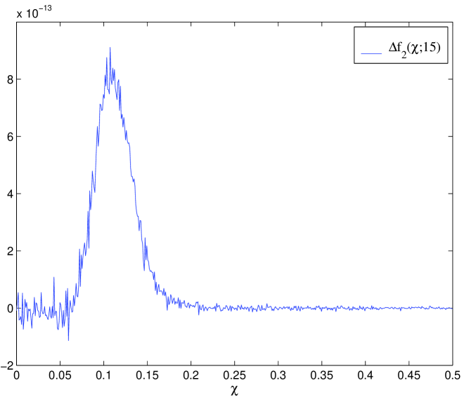
Figure 12. Absolute error in the cut profile $f_{2}(\chi;15)$. Here we plot the difference $\Delta f_{2}(\chi;15)$ of two numerical computations of $f_{2}(\chi;15)$, one based on the two–component path method and the other on the one–component path method. For the two–component method we have $N=131072=M$, while for the one–component method $P=262144$. Parameters common to both computations are $\kappa=1$, ${\tt scale}=1000$ and $p=-3$ so $l-p=5$. There are 512 $\chi$–subintervals in the plot.

We will mainly use the described integration methods for small $l\leq 10$. However, we note that via comparison with both the continued fraction expression and extended precision calculations in Mathematica, we believe that our one–component path method maintains single precision accuracy up to about $l=50$, at least insofar as zero–finding is concerned. Finally, we mention that we have carried out all integration using the Runga–Kutta–Fehlburg scheme with fixed step–size along individual path components. In light of the sufficient accuracy noted here and the next subsection, we have not found it necessary to introduce any sort of adaptive integration. Furthermore, we have not found the local truncation error estimate (stemming from comparison between the fourth and fifth–order integration schemes) provided by Runga–Kutta–Fehlburg to be a useful diagnostic for our purposes. Relying on our own accuracy checks, we have simply used the straight explicit fifth–order scheme.

2.2. Numerical evaluation of the radiation kernel

The numerical methods discussed in the last subsection work well for values of $l\leq 10$, and via (68) will allow us to directly construct sufficiently accurate sum–of–poles representations of the fdrk. Moreover, even for moderately large $l$ these methods prove useful in qualitative investigations of the outgoing solution’s analytic structure. However, when it comes to building an accurate sum–of–pole representation of the fdrk for high $l$, the described methods lack the necessary accuracy.

In this subsection we describe different methods for direct evaluation of the radiation kernel itself along the Im$\sigma$ axis, ones sufficiently accurate even for high $l$. Given accurate profiles for the real and imaginary parts of the radiation kernel along this axis, we may then extract an accurate sum–of–poles representation via a method described in Section 3.3 and due to Ref. [18]. Here we described two methods for evaluating $\hat{\omega}_{l}(\sigma;\rho_{B})$ when $\sigma$ is pure imaginary, one accurate so long as $|\sigma|\gg 0$ and the other so long as $0\neq|\sigma|\lesssim 1$. There is some interval of overlap on the Im$\sigma$ axis on which both methods are accurate and may be compared. We warn the reader that we also use the notation $\hat{\omega}_{l}(\sigma;\rho_{B})$ for the Bessel fdrk $\sigma\rho_{B}W^{\prime}_{l}(\sigma\rho_{B})/W_{l}(\sigma\rho_{B})$. In order to avoid the confusion which might arise from this dual meaning of the symbol $\hat{\omega}_{l}(\sigma;\rho_{B})$, in this subsection we sometimes adopt the following notation. For the product of $z$ with the Heun logarithmic derivative we may use

(81) $$w_{l}(z;\sigma)=zW^{\prime}_{l}(z;\sigma)/W_{l}(z;\sigma)\,,$$

while for the corresponding Bessel object we may use

(82) $$w_{l}(z)=zW^{\prime}_{l}(z)/W_{l}(z)\,.$$

Formally $w_{l}(z)=w_{l}(z;0)$, in parallel with the conventions of Section 1.3.2. For the Heun case $\hat{\omega}_{l}(\sigma;\rho_{B})=w_{l}(\sigma\rho_{B};\sigma)$, while for the Bessel case $\hat{\omega}_{l}(\sigma;\rho_{B})=w_{l}(\sigma\rho_{B})$.

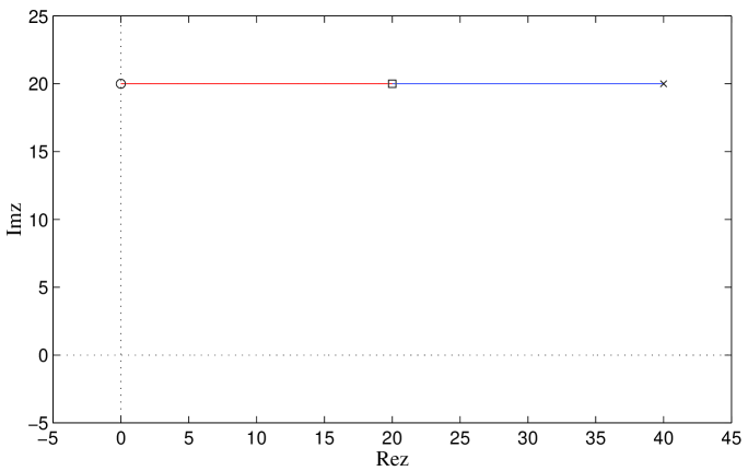
Figure 13. Two–component path in $z$–plane. The figure depicts a straight path of the type described in the text. Here we have $\rho_{B}=20$, $\sigma={\rm i}$, ${\tt scale}_{1}=20$, and ${\tt scale}_{2}=40$, so that the points $z_{1}$, $z_{2}$ and $z_{B}$ respectively correspond to the marked cross, square, and circle. Typically ${\tt scale}_{1}$ and ${\tt scale}_{2}$ will be much larger, but the values here make for a good figure.

2.2.1. Evaluation of the kernel for large imaginary frequencies

We turn first to the evaluation of $\hat{\omega}_{l}(\sigma;\rho_{B})$ for $\sigma\in{\rm i}\mathbb{R}$ and $|\sigma|\gg 0$. For the remainder of this subsection $\sigma={\rm i}y$ for real $y$. In this scenario we find it useful to again work with the complex variable $z=\sigma\rho$. As before, for a given $\sigma$ the terminal evaluation point will be denoted by $z_{B}=\sigma\rho_{B}$, and it lies on the Im$z$ axis. Consider two positive real numbers ${\tt scale}_{1}>{\tt scale}_{2}$ and associated $z$–points $z_{1}={\tt scale}_{1}+z_{B}$ and $z_{2}={\tt scale}_{2}+z_{B}$. The point $z_{1}$ is analogous to the point $z_{\infty}$ introduced before. Further consider a straight path like the one shown in Fig. 13 running through all of these points. Let us now outline the method for obtaining the value $\hat{\omega}_{l}(z_{B}/\rho_{B};\rho_{B})$, mostly considering only the model Bessel case to streamline the presentation. First, using the truncated series $\sum_{n=0}^{l-p}c_{n}z_{1}^{-n}$, we compute initial values for the ode (46). Next, we integrate the ode along the straight path from $z_{1}$ to $z_{2}$ (the first portion of the path in Fig. 13). As Re$z>0$ along this path, we again have exponential suppression of errors both in the initial conditions and due to roundoff. The result of this integration is accurate numerical values for $W_{l}(z_{2})$ and $W^{\prime}_{l}(z_{2})$, from which we can directly build a numerical value for the kernel $z_{2}W^{\prime}_{l}(z_{2})/W_{l}(z_{2})$ at this intermediary point. The assumption here is that $z_{2}$ is still large enough in modulus to ensure that the solution $W_{l}(z_{2})$ is not too large. Finally, we integrate the radiation kernel itself along the straight path from $z_{2}$ to $z_{B}$, carrying this out as follows.

Whether we are working with (44) or (46), we have an ode of the form

(83) $$\frac{{\rm d}^{2}\hat{\Phi}_{l}}{{\rm d}z^{2}}+R(z;\sigma)\frac{{\rm d}\hat{\Phi}_{l}}{{\rm d}z}+S(z;\sigma)\hat{\Phi}_{l}=0\,,$$

so that both $w_{l}(z)$ and $w_{l}(z;\sigma)$ obey a first–order nonlinear ode of the form

(84) $$\frac{{\rm d}w_{l}}{{\rm d}z}-\frac{w_{l}}{z}+\frac{w_{l}^{2}}{z}+R(z;\sigma)w_{l}+zS(z;\sigma)=0\,.$$

We use the same symbol $w_{l}$ as the dependent variable here, since as a first–order ode there is only one linearly independent solution. With the accurate value for $w_{l}(z_{2})$ at our disposal at the end of the first integration leg, we integrate this last ode from $z_{2}$ to the terminal value $z_{B}$ (the second portion of the path in Fig. 13) in order to obtain the desired complex value $w_{l}(z_{B})=z_{B}W^{\prime}_{l}(z_{B})/W_{l}(z_{B})$. For the Heun case Eq. (84) is an ode for $w_{l}(z;\sigma)=zW^{\prime}_{l}(z;\sigma)/W_{l}(z;\sigma)$, and it is again integrated from $z_{2}$ to $z_{B}$, given an accurate value for $w_{l}(z_{2};\sigma)$.

The method just described can be unstable if the terminal point $z_{B}$ lies too close to the origin. Indeed, notice that some of the terms in the ode (84) are singular at the origin, showing that finiteness of the kernel derivative at the origin depends on exact cancellation of singular terms. Round off error will spoil any such exact cancellation in an integration towards a terminal $z_{B}$ equal to or near zero. Later we demonstrate that the value $\hat{\omega}_{l}(0;\rho_{B})$ of the kernel at the origin can be computed in closed form for both the Bessel and Heun cases. This raises the possibility that the value $w_{l}(z_{B})$ —or in the Heun case the value $w_{l}(z_{B};\sigma)$— corresponding to a non–zero $|z_{B}|\ll 1$ might be numerically computed via integration of (84) out from the origin. However, our numerical experiments suggest that this is not a viable approach. Moreover, the following analytical reasoning would also seem to dash this possibility. For the Bessel $l=2$ case we have the exact expression

(85) $$zW^{\prime}_{2}(z)/W_{2}(z)=-\frac{3z+6}{z^{2}+3z+3}\,.$$

A linearization stability analysis of the Bessel–case ode (84) about this solution indicates that small perturbations of $zW^{\prime}_{2}(z)/W_{2}(z)$ grow exponentially on paths running away from the origin along the Im$z$ axis.

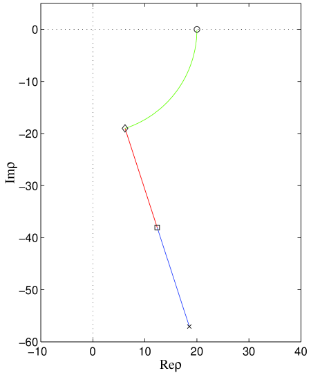
Figure 14. Three–component path in $\rho$–plane. The figure depicts an example three–component path of the type described in the text. Here we have $\rho_{B}=20$, ${\tt scale}_{1}=60$, ${\tt scale}_{2}=40$, and $\theta=-2\pi/5$ so that the points $\rho_{1}$, $\rho_{2}$, $\rho_{3}$ and $\rho_{B}$ respectively correspond to $60\exp(-{\rm i}2\pi/5)$ (cross), $40\exp(-{\rm i}2\pi/5)$ (square), $20\exp({-\rm i}2\pi/5)$ (diamond), and 20 (circle). The depicted path corresponds to a $\sigma$ value lying on the positive imaginary axis, so that between $\rho_{1}$ and $\rho_{3}$ we have Re$(\sigma\rho)>0$. Better suppression of error would be had for $\theta=-\pi/2$, in which case the portion of the path between $\rho_{1}$ and $\rho_{3}$ would lie on the negative imaginary axis. However, the final integration would then be over a longer arc, and on this final arc we do not expect to have error suppression. There seems to be some trade–off here, which is why we have kept $\theta$ as a parameter. In any case, typically ${\tt scale}_{1}$ and ${\tt scale}_{2}$ will be much larger, but the values here make for a good figure.

2.2.2. Evaluation of the kernel for small imaginary frequencies

For the reasons just laid down, we use a different method for small non–zero imaginary $\sigma$. The new method employs integration in the complex $\rho$–plane rather than the $z$–plane. We introduce new positive real numbers ${\tt scale}_{1}>{\tt scale}_{2}>\rho_{B}$, a phase factor $\exp({\rm i}\theta)$, and the following associated $\rho$–points (all in polar form): $\rho_{1}={\tt scale}_{1}*\exp({\rm i}\theta)$, $\rho_{2}={\tt scale}_{2}*\exp({\rm i}\theta)$, $\rho_{3}=\rho_{B}\exp({\rm i}\theta)$, and $\rho_{B}$. These points define a three–component path in the $\rho$–plane such as the one shown in Fig. 14. Let us now outline the new method for computing the value $\hat{\omega}_{l}(\sigma;\rho_{B})$, again mostly considering only the model Bessel case to streamline the presentation. First, using the asymptotic expansion (78), we compute initial values for the ode (77). Next, we integrate (77) along the straight ray from $\rho_{1}$ to $\rho_{2}$ (the first portion of the path in Fig. 14). We choose the angle $\theta$ such that Re$(\sigma\rho)>0$ along this path, ensuring exponential suppression of errors both in the initial conditions and due to roundoff. The result of this integration is accurate numerical values for $W_{l}(\sigma\rho_{2})$ and $W^{\rho}_{l}(\sigma\rho_{2})$, from which we can directly build a numerical value for $w_{l}(\sigma\rho_{2})$ at the intermediary point $\rho_{2}$. Similar to before, the assumption is that $\rho_{2}$ is large enough in modulus to ensure that the solution $W_{l}(\sigma\rho_{2})$ is not too large. Finally, we integrate $w_{l}(\sigma\rho)$ itself along a two–component ray–and–arc path from $\rho_{2}$ to the real point $\rho_{B}$, by way of an intermediate point $\rho_{3}$. Such a remaining two–component path is depicted in Fig. 14 as the final two portions of the curve connecting $\rho_{2}$ to $\rho_{B}$. This integration is carried out as follows.

Whether we are working with (43) or (77), we have an ode of the form

(86) $$\frac{{\rm d}^{2}\hat{\Phi}_{l}}{{\rm d}\rho^{2}}+\mathcal{R}(\rho;\sigma)\frac{{\rm d}\hat{\Phi}_{l}}{{\rm d}\rho}+\mathcal{S}(\rho;\sigma)\hat{\Phi}_{l}=0\,,$$

whence both $w_{l}(\sigma\rho;\sigma)$ and $w_{l}(\sigma\rho)$ obey a first–order nonlinear ode of the form

(87) $$\frac{{\rm d}w_{l}}{{\rm d}\rho}-\frac{w_{l}}{\rho}+\frac{w_{l}^{2}}{\rho}+\mathcal{R}(\rho;\sigma)w_{l}+\rho\mathcal{S}(\rho;\sigma)=0\,.$$

To reach this equation, we have used, for example, $w_{l}(\rho\sigma)=\rho W_{l}^{\rho}(\rho\sigma)/W_{l}(\rho\sigma)$. Given the initial value for $w_{l}(\sigma\rho_{2})$ obtained from the first leg of the integration in the last paragraph, we first integrate (87) along the straight ray from $\rho_{2}$ to $\rho_{3}$ which has the same modulus as the terminal point $\rho_{B}$. The final leg, a rotation back to the Re$\rho$ axis, is an integration of (87) along an arc from $\rho_{3}$ to $\rho_{B}$.

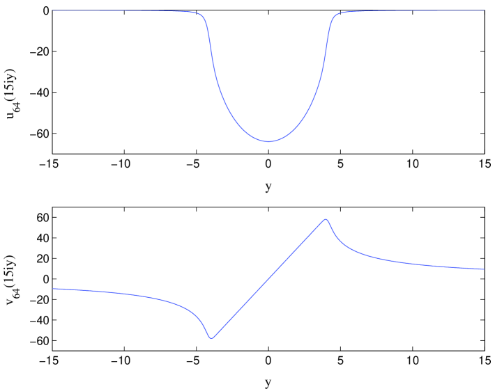
Figure 15. Bessel fdrk $\hat{\omega}_{64}({\rm i}y;15)=w_{64}(15{\rm i}y)$. Here we plot the functions $u_{64}(15{\rm i}y)=\mathrm{Re}w_{64}(15{\rm i}y)$ and $v_{64}(15{\rm i}y)=\mathrm{Im}w_{64}(15{\rm i}y)$, with the $y$ axis split into 512 subintervals. For $|y|>{\tt break}=1$ we have evaluated $\hat{\omega}_{51}({\rm i}y;15)$ using two–component integration with the following parameter values: $N=131072$, $M=131072$, ${\tt scale}_{1}=1000$, and ${\tt scale}_{2}=100$. $N$ and $M$ are respectively the number of integration steps taken along the first and second components of the path. For $|y|\leq{\tt break}$ we have evaluated $\hat{\omega}_{51}({\rm i}y;15)$ using three–component integration with the parameter values $N=131072$, $M=131072$, $P=2048$, $\theta=\pi/4$, ${\tt scale}_{1}=1000$, and ${\tt scale}_{2}=100$. $N$, $M$, and $P$ are respectively the number of integration steps taken along the first, second, and third components of the path. For both integration methods $\kappa=1$ and $p=59$. Typically, we have chosen ${\tt break}$ smaller, but now have ${\tt break}=1$ to demonstrate the three–component method.

2.2.3. Value of the kernel at the origin

For the Bessel case the origin value $\hat{\omega}_{l}(0;\rho_{B})$ of the radiation kernel is the limit $\lim_{\sigma\rightarrow 0}w_{l}(\sigma\rho_{B})$, while for the Heun case the value $\hat{\omega}_{l}(0;\rho_{B})$ is the limit $\lim_{\sigma\rightarrow 0}w_{l}(\sigma\rho_{B};\sigma)$. Whether considering the Bessel or Heun case, we may derive an exact expression for the value $\hat{\omega}_{l}(0;\rho_{B})$. Turn first to the Bessel case, where $W_{l}(\sigma\rho)=\sum^{l}_{n=0}c_{n}(\sigma\rho)^{-n}$ is of course singular at $\sigma=0$. However, with this exact expression it is easy to check that

(88) $$\lim_{\sigma\rightarrow 0}w_{l}(\sigma\rho_{B})=-l\,.$$

We stress that this calculation of $\hat{\omega}_{l}(0;\rho_{B})$ makes use of the exact form of the outgoing solution, which is not at our disposal in the Heun case. A separate recipe for getting this value, one without appeal to the exact form of $W_{l}(\sigma\rho_{B})$, goes as follows. Set $\sigma=0$ in (77), thereby reaching an ode

(89) $$\frac{{\rm d}^{2}\hat{\Phi}_{l}}{{\rm d}\rho^{2}}-\frac{l(l+1)}{\rho^{2}}\hat{\Phi}_{l}=0\$$

with solutions $\rho^{l+1}$ and $\rho^{-l}$. We now use $[\rho\partial_{\rho}\log\rho^{-l}]|_{\rho=\rho_{B}}$ as the origin value $\hat{\omega}_{l}(0;\rho_{B})$, again finding $-l$.

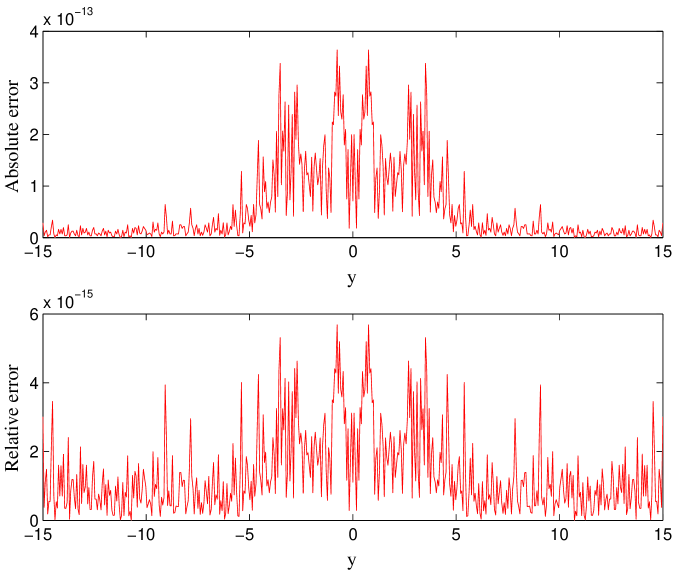
Figure 16. Error in Bessel fdrk $\hat{\omega}_{64}({\rm i}y;15)=w_{64}(15{\rm i}y)$. Here we plot the absolute error $|\Delta w_{64}(15{\rm i}y)|$ as well as the relative error $|\Delta w_{64}(15{\rm i}y)|/|w_{64}(15{\rm i}y)|$. These errors have been computed against the “exact” $w_{64}(15{\rm i}y)$ generated with the continued fraction expression (79). Parameters are the same as in Fig. 15.

Let us turn to the Heun case and follow this recipe for getting the value $\hat{\omega}_{l}(0;\rho_{B})$. We set $\sigma=0$ in (43), obtaining the following ode:

(90) $$\frac{{\rm d}^{2}\hat{\Phi}_{l}}{{\rm d}\rho^{2}}+\left[-\frac{1}{\rho}+\frac{1}{\rho-1}\right]\frac{{\rm d}\hat{\Phi}_{l}}{{\rm d}\rho}+\left[\frac{\kappa}{\rho^{2}}-\frac{\kappa+l(l+1)}{\rho(\rho-1)}\right]\hat{\Phi}_{l}=0\,,$$

Both solutions to this equation may be expressed in terms of infinite series in inverse $\rho$. The one corresponding to $\rho^{-l}$ above has the form

(91) $$\sum_{n=0}^{\infty}a_{n}\rho^{-(l+n)}\,,$$

where $a_{0}=1$ and

(92) $$a_{n+1}=\frac{(l+n)(l+n+2)+\kappa}{(l+n+1)(l+n+2)-l(l+1)}\,a_{n}\,.$$

The series is positive and absolutely convergent for all $\rho>1$. We then have

(93) $$\hat{\omega}_{l}(0;\rho_{B})=-\sum^{\infty}_{n=0}(l+n)a_{n}\rho^{-n}_{B}\Big{/}\sum^{\infty}_{n=0}a_{n}\rho^{-n}_{B}$$

as our concrete expression for the value in question. Notice that this value approaches $-l$ in the $\rho_{B}\rightarrow\infty$ limit as expected.

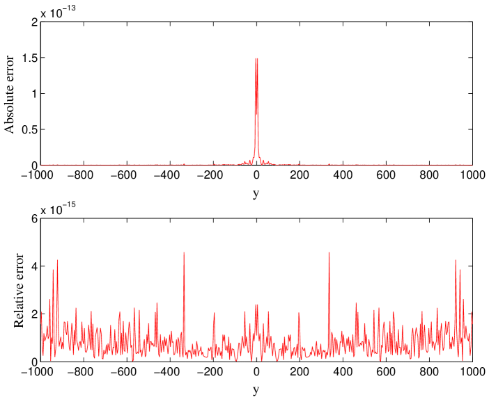
Figure 17. Error in Bessel fdrk $\hat{\omega}_{64}({\rm i}y;15)$. These are essentially the same plots as those in Fig. 16, save that here we have a larger $y$–interval.

2.2.4. Accuracy of the numerical evaluation

Fig. 15 depicts the real part $u_{64}(15{\rm i}y)$ and the imaginary part $v_{64}(15{\rm i}y)$ of the Bessel fdrk $\hat{\omega}_{64}({\rm i}y;15)=w_{64}(15{\rm i}y)$ along the Im$\sigma$ axis for $l=64$ and $\rho_{B}=15$. We have generated these plots using the methods described in this subsection, and have listed other parameters set while obtaining them in the figure caption. To examine the accuracy of these numerical profiles, we may compare them with corresponding profiles obtained via the continued fraction expansion (79). We consider the profiles stemming from the continued fraction expansion as the “exact” ones. With the two sets of profiles, one may compute corresponding absolute and relative error measures. We plot these errors in Fig. 16 and Fig. 17 (the second being a pull–back of the first). From these figures we conclude that our numerical methods evaluate $w_{64}(15{\rm i}y)$ with an absolute supremum error less than $10^{-12}$ and a relative supremum error less than $10^{-14}$, at least for $|y|<1000$. For the Bessel case at hand we have found comparable error bounds associated with all other values of $l\in\{10,11,\dots,64\}$, although we note that the corresponding $y$–interval needs to shrink by as much as an order of magnitude to maintain these bounds for $l=10$.

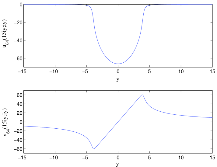
Figure 18. Heun fdrk $\hat{\omega}_{64}({\rm i}y;15)=w_{64}(15{\rm i}y;{\rm i}y)$. Here we plot the functions $u_{64}(15{\rm i}y;{\rm i}y)=\mathrm{Re}w_{64}(15{\rm i}y;{\rm i}y)$ and $v_{64}(15{\rm i}y;{\rm i}y)=\mathrm{Im}w_{64}(15{\rm i}y;{\rm i}y)$. All parameters in these plots match those listed in Fig. 15 depicting the Bessel fdrk.

Fig. 18 depicts the real part $u_{64}(15{\rm i}y;{\rm i}y)$ and the imaginary part $v_{64}(15{\rm i}y;{\rm i}y)$ of the Heun fdrk $\hat{\omega}_{64}({\rm i}y;15)=w_{64}(15{\rm i}y;{\rm i}y)$ along the Im$\sigma$ axis. We have again chosen the representative case $l=64$ and $\rho_{B}=15$, setting the rest of the parameters to the same values used to generate the Bessel profiles depicted in Fig. 15. Note that the two sets of profiles are qualitatively very similar. However, they are different. In particular, now the real part has a minimum value of $-66.2816976576098$ rather than $-64$. For the Heun case at hand we have no analog of the continued fraction expansion with which to check the accuracy of the profiles. Nevertheless, at least for $y$ values of order unity, we can perform an accuracy check by comparing the two–component and three–component path methods for evaluating the kernel. Such a comparison is shown in Fig. 19. With the two numerically obtained kernels we form an absolute error measure $|\Delta w_{64}(15{\rm i}y;{\rm i}y)|$ and also a relative error measure $|\Delta w_{64}(15{\rm i}y;{\rm i}y)|/|w_{64}(15{\rm i}y;{\rm i}y)|$, over $y\in[0.5,8]$ for both. In the denominator of the relative error, we happen to have used the kernel stemming from the three–component method. Fig. 19 displays plots of both error measures. Note that poor performance for the three–component method is evident in the right portions of the plots. For the three–component method the length of the third and final integration path grows with $y$. Therefore, for large $y$ one expects a corresponding loss of precision for the three–component method.

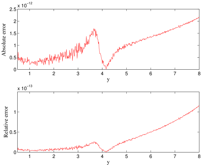
Figure 19. Error in Heun fdrk $\hat{\omega}_{64}({\rm i}y;15)=w_{64}(15{\rm i}y;{\rm i}y)$. Here we plot the absolute error measure $|\Delta w_{64}(15{\rm i}y;{\rm i}y)|$ and the relative error measure $|\Delta w_{64}(15{\rm i}y;{\rm i}y)|/|w_{64}(15{\rm i}y;{\rm i}y)|$ described in the text. We have $y\in[0.5,8]$ for both. All other parameters set in generating these plots are the same as those listed in the caption of Fig. 15.

3. Sum–of–poles representation of the radiation kernel

In this section we focus on both exact and approximate representation of the fdrk $\hat{\omega}_{l}(\sigma;\rho_{B})$ as a sum of poles. In the first subsection we qualitatively discuss the exact representation (68) of the fdrk as a (continuous and discrete) sum of poles, highlighting what we believe to be its main features. In the second subsection we document our particular numerical construction of the fdrk as a sum of poles, and give an analysis of its numerical error. We stress that from a theoretical standpoint we are conjecturing that the Schwarzschild fdrk —built from the Heun function $W_{l}(z;\sigma)$— admits the representation (68), although we do provide compelling numerical evidence for a representation of this form. This is in contrast to the case of the flatspace fdrk —built from the Bessel function $W_{l}(z)$— which we theoretically know admits such a representation [18]. Since for us the representation (68) of the Schwarzschild fdrk is ultimately conjecture, there is more need to painstakingly justify it numerically, and we do so in the second subsection. In the third subsection we turn to kernel compression, by which we mean approximation of the fdrk by a proper rational function $P(\sigma)/Q(\sigma)$ which is itself a sum of poles. In the first and second subsections we consider only the $\jmath=0$ ($\kappa=1$) case, but also consider the $\jmath=2$ ($\kappa=-3$) case in subsection three. As yet, we have not examined the $j=1$ ($\kappa=0$) case corresponding to electromagnetic radiation.

In this section and in the simulations we describe later, we have almost exclusively worked with an outer boundary radius $\rho_{B}\in[15,25]$, corresponding to a physical outer boundary radius $r_{B}\in[30\mathrm{m},50\mathrm{m}]$. Therefore, were we considering a more general isolated source of gravitational radiation, one with gravitational radius $2\mathrm{m}$, then the boundary two–sphere $B$ would be located outside of the strong–field region as defined by Thorne [64]. Moreover, for wave simulation on a fixed background as we consider here, the location of $B$ corresponds to a metric coefficient $F(\rho_{B})$ from (14) in the range $0.9\overline{33}\leq F(\rho_{B})\leq 0.96$. Whence $B$ lies in a region where the Schwarzschild metric is flat up to small correction. The robc described in Section 1.4 are not tied to the weak–field region. However, for this region our numerical methods for examining/constructing the fdrk are accurate.

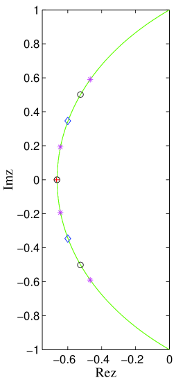
Figure 20. Scaled zeros of MacDonald functions. Here we plot scaled zeros $(l+1/2)^{-1}k_{l,n}$ for $l=1,2,3,4$. The cross is the scaled zero of $K_{1/2}(z)$, the diamonds are the scaled zeros of $K_{3/2}(z)$, the circles are the scaled zeros of $K_{5/2}(z)$, and the stars are the scaled zeros of $K_{7/2}(z)$. To the eye these zeros, corresponding as they do to small $l$ values, already lie close to the curve $\mathcal{C}$ shown and described in both the text and the caption of Figure 8 in Section 2.1.3. As $l$ gets large the scaled zeros $(l+1/2)^{-1}k_{l,n}$ lie closer and closer to $\mathcal{C}$.

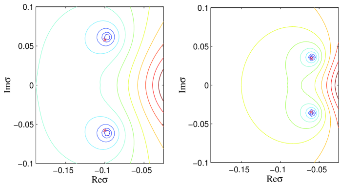
Figure 21. Zeros of $W_{2}(15\sigma;\sigma)$ and $W_{2}(25\sigma;\sigma)$. The lefthand plot shows contour lines of $\log|W_{2}(15\sigma;\sigma)|$, and the righthand one shows contour lines of $\log|W_{2}(25\sigma;\sigma)|$. The logarithm mollifies the singularity at the origin, distributing contour lines more evenly. Notice that the zero locations are closer to the origin in the righthand plot. In the lefthand plot and the righthand plot we have also respectively marked as crosses the zeros of the Bessel functions $W_{2}(15\sigma)=1+3(15\sigma)^{-1}+3(15\sigma)^{-2}$ and $W_{2}(25\sigma)=1+3(25\sigma)^{-1}+3(25\sigma)^{-2}$. Perhaps evident even to the eye, the Bessel and Heun zeros lie closer to each other in the righthand plot (corresponding to the larger value of $\rho_{B}$).

3.1. Qualitative study of pole locations and cut profile

Using the one–component path method described in Section 2.1.3, we first turn to the analytic structure of $W_{l}(\sigma\rho_{B};\sigma)$ as a function of frequency $\sigma$ in the lefthalf plane, assuming that a zero of this function corresponds to a pole location appearing in (68). Using the same method, we then draw some quick observations concerning the cut profile $f_{l}(\chi;\rho_{B})$ in (68). We mainly focus on the restricted parameter space $\mathbb{S}$ determined by $\rho_{B}\in[15,25]$ and $0\leq l\leq 10$, but also make mention of some remarkable features which crop up for other parameter values outside of this space. Our parameter space $\mathbb{S}$ has been chosen with the following reasons in mind. First, its $\rho_{B}$ interval is as discussed in the last paragraph. Second, it includes the first few values of $l$, which we want to single out for special attention. Third (and related to the first two), it avoids by design the aforementioned remarkable features. We stress that our discussion in this first subsection is mostly qualitative and amounts to a collection of conjectures without substantial numerical or analytical proof. Although we are bypassing a truly thorough study of some interesting phenomena, we do not believe these phenomena to be directly relevant for numerical implementation of robc (further remarks on this point to follow).

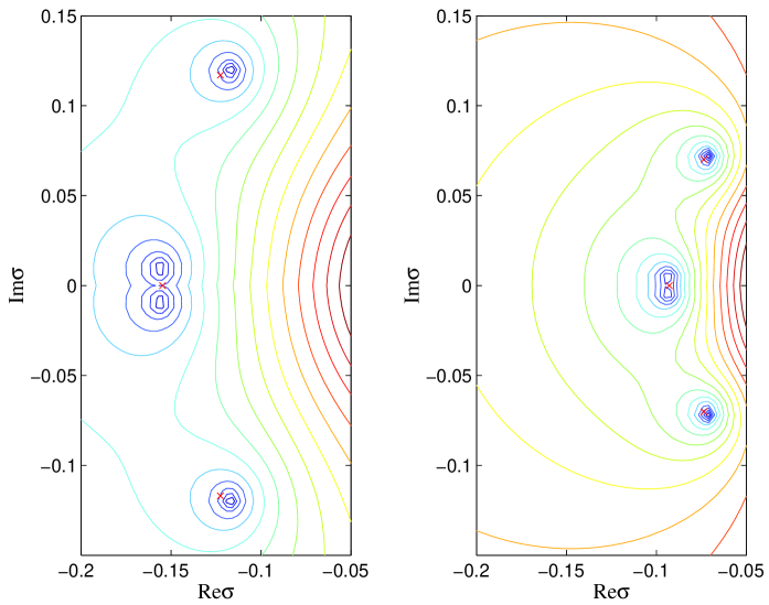
Figure 22. Zeros of $W_{3}(15\sigma;\sigma)$ and $W_{3}(25\sigma;\sigma)$. The lefthand plot shows contour lines of $\log|W_{3}(15\sigma;\sigma)|$, and the righthand one shows lines of $\log|W_{3}(25\sigma;\sigma)|$. Again, crosses mark the corresponding Bessel zeros. Notice in the lefthand plot that the single real Bessel zero corresponds to a pair of zeros in the Heun case. Actually, in the righthand plot there are also two distinct Heun zeros, each one near the Bessel zero lying on the real axis, but the resolution is almost too low to see them as distinct.

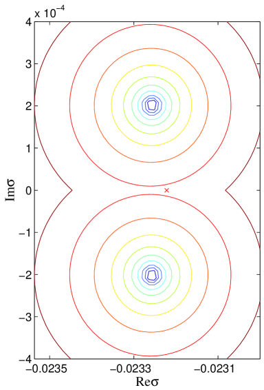
Figure 23. Zeros of $W_{3}(100\sigma;\sigma)$. Here we plot contour lines of $\log|W_{3}(100\sigma;\sigma)|$. Note that two zeros of $W_{3}(100\sigma;\sigma)$ lie outside of the plot, as we focus on the pair of zeros closest to the real axis. The red cross is a zero of $W_{3}(100\sigma)$. We might gather from this plot that the feature associated with odd $l$ and discussed in the text persists as $\rho_{B}$ gets large.

3.1.1. Zeros of the outgoing solution as a function of $\sigma$

Recall that in Section 2.1.3 we denoted by $\{k_{l,n}:n=1,\cdots,l\}$ the zero set of the MacDonald function $K_{l+1/2}(z)$ which is also the zero set of $W_{l}(z)$. With this notation the zeros in $\sigma$ of $W_{l}(\sigma\rho_{B})$ are then simply the $k_{l,n}/\rho_{B}$. Let us collect several facts concerning such sets, summarizing results derived or listed in Refs. [61, 18, 63, 21]. First, for even $l$ these zeros come in complex–conjugate pairs, while for odd $l$ they again come in complex–conjugate pairs save for a lone zero which lies on the negative Re$\sigma$ axis. Second, the scaled zeros $(l+1/2)^{-1}k_{l,n}$ lie close to the asymptotic curve $\mathcal{C}$ introduced in Section 2.1.3. See Fig. 20 for a graphical demonstration of this claim. Hence, for each $l$ one may imagine the zeros distributed in a crescent pattern in the lefthalf $\sigma$–plane. As concrete examples, the zeros of $W_{2}(15\sigma)$ are approximately $-0.1000\pm{\rm i}0.0577$, while those of $W_{3}(15\sigma)$ are approximately $-0.1226\pm{\rm i}0.1170$ and $-0.1548+{\rm i}0$. Respectively, these zero sets are marked by crosses in the lefthand plots of Figs. 21 and 22.

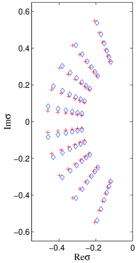
Figure 24. Zeros of $W_{10}(\sigma\rho_{B};\sigma)$ and $W_{10}(\sigma\rho_{B})$. Here we plot zeros of these functions for $\rho_{B}=15,17,19,21,23,25$. The outermost crescent of diamonds are the zeros of $W_{10}(15\sigma;\sigma)$, while the innermost crescent of diamonds are the zeros of $W_{10}(25\sigma;\sigma)$. The outermost crescent of crosses are the zeros of $W_{10}(15\sigma)$, while the innermost crescent of crosses are the zeros of $W_{10}(25\sigma)$.

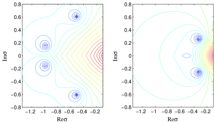
Figure 25. Zeros of $W_{2}(\sigma\rho_{B};\sigma)$. On the left we have a plot of $\log|W_{2}(2\sigma;\sigma)|$ and on the right one of $\log|W_{2}(4\sigma;\sigma)|$, demonstrating that a new pair of zeros is created between $\rho_{B}=4$ and $\rho_{B}=2$. The initial stages of this creation are perhaps evident in the rightmost plot.

Zeros for chosen parameter space. Dealing with $W_{l}(\sigma\rho_{B};\sigma)$ as a function of $\sigma$ in the Heun scenario, we have denoted the zeros of this function by $\sigma_{l,n}=\sigma_{l,n}(\rho_{B})$. Over the range $\mathbb{S}$ of parameters mentioned above, the zeros $\sigma_{l,n}$ behave qualitatively similar to the zeros $k_{l,n}/\rho_{B}$ of $W_{l}(\sigma\rho_{B})$, save for one key difference associated with odd $l$. Fig. 21 displays contour plots showing zero locations for $W_{2}(15\sigma;\sigma)$ and $W_{2}(25\sigma;\sigma)$. Likewise, Fig. 22 displays contour plots showing zero locations for $W_{3}(15\sigma;\sigma)$ and $W_{3}(25\sigma;\sigma)$. These plots exhibit the main features associated with the zeros of $W_{l}(\sigma\rho_{B};\sigma)$ over $\mathbb{S}$. To the eye, apparent zero locations in these plots nearly match zero locations (marked as crosses) for the corresponding Bessel functions. However, as shown in Fig. 22 and also noted in the figure caption, there is a key difference associated with odd $l$. To appreciate the difference, compare the zeros of $W_{3}(15\sigma)$ with those of $W_{3}(15\sigma;\sigma)$. Notice that the single zero of $W_{3}(15\sigma)$ lying on the negative Re$\sigma$ axis corresponds to two zeros of $W_{3}(15\sigma;\sigma)$, one lying just above and the other just below the negative Re$\sigma$ axis. This is a generic feature belonging to all odd values of $l\in\{1,3,5,7,9\}$ and $\rho_{B}\in[15,25]$ considered here. Therefore, for the Heun scenario and the parameter space $\mathbb{S}$ at hand there are an even number of zeros whether $l$ is even or odd. Moreover, we believe that this feature (of a pair of complex–conjugate zeros lying close to the real axis and together corresponding to a single Bessel zero) persists as $\rho_{B}$ gets large, as evidenced by Fig. 23 and its caption. More precisely, if $N_{l}=N_{l}(\rho_{B})$ denotes the number of zeros belonging to $W_{l}(\sigma\rho_{B};\sigma)$, then for each $l\in\{0,\dots,10\}$ we observe that $N_{l}$ is constant on $[15,25]$ with $N_{0}=0$, $N_{1}=2=N_{2}$, $N_{3}=4=N_{4}$, $N_{5}=6=N_{6}$, $N_{7}=8=N_{8}$, and $N_{9}=10=N_{10}$. Our conjecture is that each $N_{l}$ is also the same constant on $[15,\infty)$.

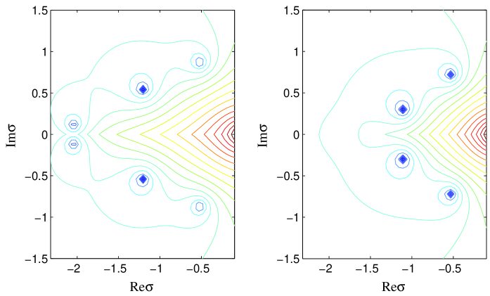
Figure 26. Zeros of $W_{2}(\sigma\rho_{B};\sigma)$. On the left we have a plot of $\log|W_{2}(1.5\sigma;\sigma)|$ and on the right one of $\log|W_{2}(1.75\sigma;\sigma)|$, demonstrating that a second new pair of zeros is created between $\rho_{B}=1.75$ and $\rho_{B}=1.5$. As $\rho_{B}\rightarrow 1^{+}$ more and more zero pairs are created.

Asymptotics of zeros. We discuss two asymptotic regimes for zero locations: one large $\rho_{B}$ at fixed $l$ and the other large $l$ at fixed $\rho_{B}$. Turning to the first regime, we conjecture that the zeros $\sigma_{l,n}(\rho_{B})$ approach the Bessel zeros $k_{l,n}/\rho_{B}$ as $\rho_{B}$ becomes large. That is to say, the first term in the asymptotic expansion (66) is

(94) $$\sigma_{l,n,1}=k_{l,n}.$$

Fig. 24 is a typical piece of graphical evidence indicating such behavior. Using the zero locations shown in this figure, we have confirmed for each $n$ that $\big{|}\sigma_{10,n}(\rho_{B})-k_{10,n}/\rho_{B}\big{|}=O(\rho_{B}^{-2})$ over $[15,25]$, in parallel with the first two terms in (66).

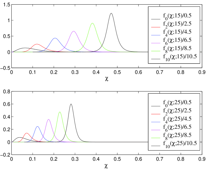
Figure 27. Even cut profiles scaled by order for $\rho_{B}=15$ and $25$. Here, for example, $f_{0}(\chi;15)/0.5$ is on the far left, and $f_{10}(\chi;15)/10.5$ on the far right.

Now turning to the second asymptotic regime, we remark on the order scaling of Heun zeros as $l$ becomes large. We have observed that the scaled zeros $(l+1/2)^{-1}\sigma_{l,n}$ tend to accumulate on the same fixed curve $\mathcal{C}_{\rho_{B}}$ as $l$ becomes large. For example, using the 20 scaled zeros $\sigma_{20,n}(15)/20.5$ to hint at a candidate $\mathcal{C}_{15}$, one finds that —to the eye at least— all scaled zeros for $l<20$ lie on this curve. Of course $\mathcal{C}_{\rho_{B}}$ is of a different shape than the dilated curve $\mathcal{C}/\rho_{B}$, although choosing a still larger fixed $\rho_{B}$ value yields better agreement between the two curves. That is to say, consistent with the first type of asymptotic behavior discussed, we have $\rho_{B}\mathcal{C}_{\rho_{B}}\rightarrow\mathcal{C}$ holding pointwise as $\rho_{B}\rightarrow\infty$. We are not confident that this order scaling is robust for very large $l$.

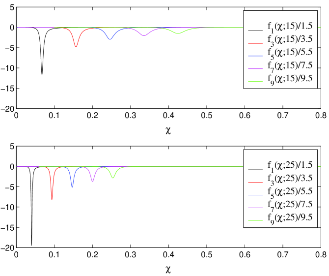
Figure 28. Odd cut profiles scaled by order for $\rho_{B}=15$ and $25$. Here, for example, $f_{1}(\chi;15)/1.5$ is on the far left, and $f_{9}(\chi;15)/9.5$ on the far right.

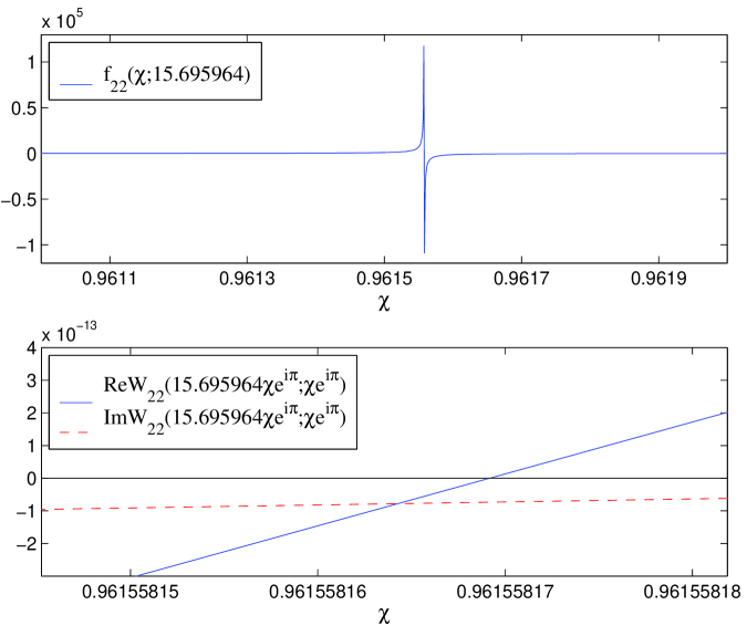
Figure 29. Blow–up in cut profile near a critical value. The value $15.695964$ is close to the critical value $\rho_{B}^{c_{1}}$ for $l=22$. See the text for more description.

Zero pair creation as $\rho_{B}$ approaches unity. We have claimed that over the $\rho_{B}$ interval $[15,25]$ Heun zero behavior is similar to Bessel zero behavior, save for the aforementioned curious feature concerning odd $l$. As mentioned, we believe our claim remains true over $[15,\infty)$ for all low $l$ here of interest. However, as we now argue, the number $N_{l}$ of zeros for a given $l$ is not conserved as $\rho_{B}\rightarrow 1^{+}$. The behavior we have noticed is the following.

For each value $l\in\{0,\dots,10\}$ there is a critical value $\rho_{B}^{c_{1}}$ of $\rho_{B}$ (less than $15$ of course) for which a new pair of zeros is created on the negative Re$\sigma$ axis, the branch cut. Below that there is yet another critical value $\rho_{B}^{c_{2}}$ for which yet another new pair of zeros is created on the negative Re$\sigma$ axis, and so on. Therefore, it would seem that as a function $N_{l}(\rho_{B})$ is step–like and blows up as $\rho_{B}\rightarrow 1^{+}$. Let us remark on the nature of the zero lying on the branch cut for a critical value $\rho_{B}^{c_{j}}$. As $\rho_{B}$ is increased past $\rho_{B}^{c_{1}}$, say, two zeros appear to collide on the branch cut. However, they do not merge into a double zero, rather they pass “over and under each other,” with each zero remaining on its own analytic neighborhood continued across the branch cut.

In Figs. 25 and 26 we document the creation of the first and second new zero pairs for $W_{2}(\sigma\rho_{B};\sigma)$ associated with decreasing $\rho_{B}$ from $4$ down to $1.5$. In Table 4 we have listed approximations to the critical values $\rho_{B}^{c_{1}}$ for $l\in\{0,\dots,10\}$. Using $\sigma=\chi\exp(\mathrm{i}\pi)$ along the negative Re$\sigma$ axis, the table also lists approximate values for the location $\chi^{c_{1}}$ of each zero–pair creation. We have obtained these numbers using the method discussed below in reference to Fig. 29. All of the approximate critical values in the table are well below our $\rho_{B}$ interval $[15,25]$; however, for higher $l$ values creation of a zero pair can occur in our interval. For instance, in what follows we determine that creation of the first new zero pair for $l=22$ occurs for $\rho^{c_{1}}_{B}\simeq 15.70$ and $\chi^{c_{1}}\simeq 0.96$.

$l$	0	1	2	3	4	5	6	7	8	9	10
$\rho^{c_{1}}_{B}$	$1.49$	$1.52$	$2.52$	$2.06$	$3.81$	$2.67$	$5.11$	$3.31$	$6.44$	$3.97$	$7.75$
$\chi^{c_{1}}$	$0.63$	$1.31$	$0.79$	$1.49$	$0.85$	$1.60$	$0.89$	$1.67$	$0.91$	$1.71$	$0.92$

Table 4. Approximate critical values of $\rho_{B}$. Here we list rough values corresponding to the creation of the first new zero pair for $W_{l}(\sigma\rho_{B};\sigma)$. For example, as $\rho_{B}$ is lowered from $1.5$ to $1.48$, the number $N_{0}$ of zeros for $W_{0}(\sigma\rho_{B};\sigma)$ jumps from 0 to 2. We also list approximate values for the location $-\chi^{c_{1}}$ of each zero–pair creation, again with $\pm 0.01$ error bounds.

3.1.2. Parameter dependence of the cut profile

Let us now discuss the cut profile $f_{l}(\chi;\rho_{B})$ appearing in the representation (68) of the fdrk. We first remark on the behavior of the profile over the chosen parameter range $\mathbb{S}$, and then turn to exceptional behavior associated with critical parameter values lying outside $\mathbb{S}$.

Behavior over the chosen parameter range. For $0\leq l\leq 10$ and for $\rho_{B}=15$ and $25$ we plot scaled even profiles in Fig. 27 and scaled odd profiles in Fig. 28. The scaling allows us to view all profiles on the same plot. Notice that the order–scaling is different for even and odd cases. As $\rho_{B}$ is increased towards $25$, the other endpoint of our interval, all of these profiles retain their shape; however, both their maximum value (in absolute value) and the essential window of their support vary.

Cauchy principal value. The chosen parameter space $\mathbb{S}$ has been carefully tailored to avoid the exceptional situation where a zero lies on the branch cut. However, over our $\rho_{B}$ interval $[15,25]$, we shall of course be interested in $l$ values higher than $10$, and on this interval zero pair creation is an issue for such $l$. A glance at the form (80) of the cut profile $f_{l}(\chi;\rho_{B})$ given earlier indicates that a negative real zero $\sigma=\exp({\rm i}\pi)\chi$ of $W_{l}(\sigma\rho_{B};\sigma)$ should give rise to a singular cut profile.

For the aforementioned exceptional case $l=22$ and $\rho_{B}^{c_{1}}\simeq 15.70$, we depict the profile blow–up in Fig. 29. In the top plot we have the cut profile $f_{22}(\chi;15.695964)$, where $15.695964$ is approximately the critical value $\rho_{B}^{c_{1}}$ of $\rho_{B}$ corresponding to the creation of the first new zero pair for the function $W_{22}(\sigma\rho_{B};\sigma)$. For $\rho_{B}$ values larger than $\rho_{B}^{c_{1}}$ the function has $22$ zeros, but as $\rho_{B}$ is lowered below $\rho_{B}^{c_{1}}$ a new pair of zeros appears from the branch cut. The lower plot depicts Re$W_{22}(15.695964\sigma;\sigma)$ (solid line) and Im$W_{22}(15.695964\sigma;\sigma)$ (dotted line) as well as their intersection point below the zero line. For $\rho_{B}=15.695962$ this intersection point lies above zero, while for $\rho_{B}=15.695966$ it lies below zero. As this intersection point appears to move smoothly with varying $\rho_{B}$, we conjecture the existence of a zero on the branch cut for a critical $\rho_{B}^{c_{1}}$ between $\rho_{B}=15.695962$ and $\rho_{B}=15.695966$ (actually we know it lies between $\rho_{B}=15.695962$ and $\rho_{B}=15.695964$). Our guess at the value, $\rho_{B}=15.695964$, should be within $2\times 10^{-6}$ of the true $\rho_{B}^{c_{1}}$. Furthermore, we note that for $\rho_{B}$ slightly above the critical value the profile $f_{22}(\chi;\rho_{B})$ is a positive peak like one in Fig. 27, but as $\rho_{B}$ is lowered past $\rho_{B}^{c_{1}}$ the profile transitions to a negative (and sharper) peak like one in Fig. 28.

Despite the blow–up discussed in the last paragraph, we emphasize that along the Im$\sigma$ axis, the fdrk $\hat{\omega}_{22}({\rm i}y;\rho_{B})$ itself changes smoothly as $\rho_{B}$ varys across $\rho_{B}^{c_{1}}$. Indeed, the pieces Re$\hat{\omega}_{22}({\rm i}y;\rho_{B})$ and Im$\hat{\omega}_{22}({\rm i}y;\rho_{B})$ may be computed either via the representation (68) or numerically via the methods outlined in Section 2.2. Using the latter methods, we observe that both pieces vary smoothly as $\rho_{B}$ varys across the critical value $\rho_{B}^{c_{1}}$. We therefore offer the following conjecture. Although the cut profile $f_{22}(\chi;\rho_{B})$ is singular at a particular point $\chi_{c_{1}}\simeq 0.96$ when $\rho_{B}=\rho_{B}^{c_{1}}\simeq 15.70$, the corresponding integral contribution

(95) $$-\frac{1}{\pi}\int^{\infty}_{0}\frac{f_{22}(\chi;\rho_{B})}{{\rm i}y+\chi}{\rm d}\chi$$

to $\hat{\omega}_{22}({\rm i}y;\rho_{B})$ varys smoothly as $\rho_{B}$ varys across $\rho_{B}^{c_{1}}$. This would seem to indicate that $f_{22}(\chi;\rho_{B}^{c_{1}})/({\rm i}y+\chi)$ has a distributional interpretation, and we believe its integral to be defined in the sense of Cauchy Principal Value. The nearly antisymmetrical blow–up in the top plot of Fig. 29 is in accord with this conjecture.

3.2. Numerical construction of the radiation kernel

We now document our numerical construction of the representation (68) over the chosen parameter space $\mathbb{S}$, also discussing in detail the accuracy of the construction.

3.2.1. Construction for chosen parameter space

To obtain the numerical kernel, we have used the one–component path method described in Section 2.1.3 both to obtain pole locations and strengths as well as the cut profile for certain parameter choices. Let us first discuss our treatment of the poles.

Construction of pole locations and strengths. Let a choice of $l\in\{0,\dots,10\}$ remain fixed throughout this paragraph. We choose nine Chebyshev points $\{1/\rho_{B}^{k}:k=0,1,\dots,8\}$ on the interval $[1/25,1/15]$. That is to say, the formula

(96) $$2\xi_{B}^{k}=0.7+0.04+(0.7-0.04)\cos[\pi(2k+1)/(2n+2)]\,.$$

determines the nine numbers $\xi^{k}_{B}=1/\rho^{k}_{B}$. Our choice of nine Chebyshev points suffices for our purposes, although we make no claim that nine is the optimal number of points. Next, for each $k$ we have used the secant algorithm to find the zero set $\{\sigma_{l,n}(\rho_{B}^{k})\}$ of $W_{l}(\sigma\rho_{B}^{k};\sigma)$. Then, at fixed $l$ and $n$ we interpolate each function $\sigma_{l,n}(\rho_{B})$ by an eighth degree Chebyshev polynomial $T_{l,n}(1/\rho_{B})$ in inverse $\rho_{B}$, so that this polynomial approximates $\sigma_{l,n}(\rho_{B})$ on the interval $[15,25]$. On the same interval, we approximate the pole strengths $\alpha_{l,n}(\rho_{B})$ by $T^{\prime}_{l,n}(1/\rho_{B})/\rho_{B}$, where here the prime ^′ denotes ${\rm d}/{\rm d}\xi_{B}$ differentiation.

Construction of the cut profile. Given any small positive $\eta$, say $\simeq 10^{-12}$, we assume the existence of corresponding finite integration limits, $\chi_{\rm min}$ (which may or may not be $0$) and $\chi_{\rm max}$, such that the integral

(97) $$-\frac{1}{\pi}\int_{\chi_{\rm min}}^{\chi_{\rm max}}\frac{f_{l}(\chi;\rho_{B})}{{\rm i}y+\chi}{\rm d}\chi$$

approximates the true value

(98) $$-\frac{1}{\pi}\int_{0}^{\infty}\frac{f_{l}(\chi;\rho_{B})}{{\rm i}y+\chi}{\rm d}\chi$$

to within relative error $\eta$ uniformly for $y\in\mathbb{R}$. We stress that this is an assumption, although one apparently true for the analogous cut profiles stemming from integral order ($\nu=l+1/2=n$) Bessel functions $W_{(n-1/2)}(\sigma\rho_{B})$, as shown in the fourth section of [18]. In practice we have “eyeballed” the integration window $[\chi_{\rm min},\chi_{\rm max}]$, for example referring to Figure 3 of Section 1.4.2, we have chosen $[0.0005,1.125]$ for $l=2$ and $\rho_{B}=15$. The correctness of our guess will be confirmed when we later examine the accuracy of the kernel. Finally, to obtain the cut contribution to the value $\hat{\omega}_{l}({\rm i}y;\rho_{B})$ for a given $y$, we discretize the integral (97) via the Simpson rule. For the profile in the aforementioned figure we have used 1024 subintervals. Values $f_{l}(\chi_{j};\rho_{B})$ belonging to nodes $\chi_{j}$ in the corresponding discrete sum are computed with the one–component path method. Since for our chosen parameter range the considered profiles appear to be of definite sign, we expect that these sums are not plagued by cancellation error.

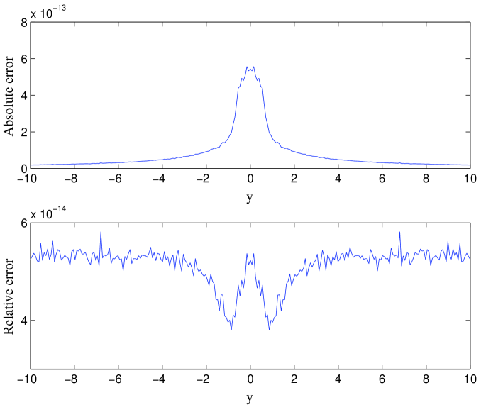
Figure 30. Error in Heun fdrk $\hat{\omega}_{10}({\rm i}y;15)=w_{10}(15{\rm i}y;{\rm i}y)$. With $256$ subintervals of the $y$ direction, we plot the absolute error $|\Delta w_{10}(15{\rm i}y;{\rm i}y)|$ and a relative error $|\Delta w_{10}(15{\rm i}y;{\rm i}y)|/|w_{10}(15{\rm i}y;{\rm i}y)|$ described in the text.

The foregoing construction of the cut contribution is applicable for a fixed value of $\rho_{B}$, whereas our construction for poles yielded locations and strengths over the whole $\rho_{B}$ interval $[15,25]$. In order to handle the cut contribution over the whole interval, we again introduce the nine Chebyshev points $\{1/\rho_{B}^{k}:k=0,1,\dots,8\}$, and —for each $\chi_{j}$ integration node— construct an eighth degree polynomial in $1/\rho_{B}$ which interpolates $f_{l}(15\chi_{j}/\rho_{B};\rho_{B})$. Notice that we are also scaling the integration nodes $\chi_{j}$ associated with $\rho_{B}=15$ [and determined by the choice of $\chi_{\rm min}$ and $\chi_{\rm max}$ as well as the number of subintervals chosen to evaluate the integral (97) via Simpson’s rule].

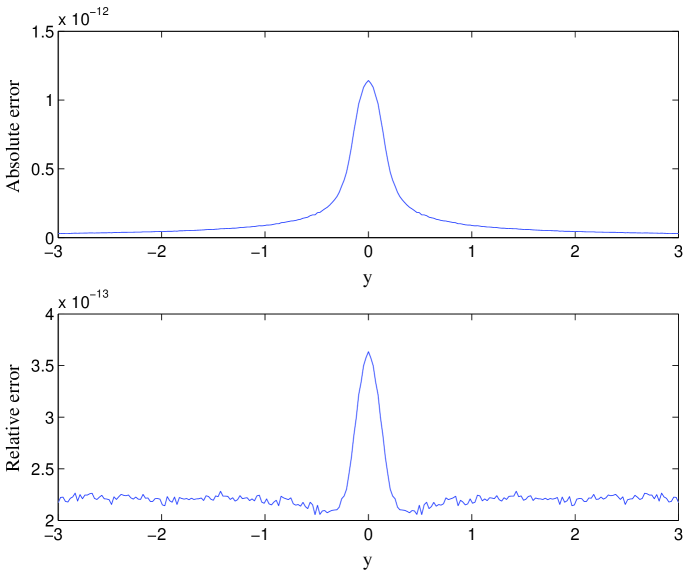
Figure 31. Error in Heun fdrk $\hat{\omega}_{3}({\rm i}y;15)=w_{3}(15{\rm i}y;{\rm i}y)$. Again with $256$ subintervals of $y$, we plot the absolute error $|\Delta w_{3}(15{\rm i}y;{\rm i}y)|$ and a relative error $|\Delta w_{3}(15{\rm i}y;{\rm i}y)|/|w_{3}(15{\rm i}y;{\rm i}y)|$ described in the text.

3.2.2. Accuracy of the construction

We check the accuracy of our numerical kernel in two ways, and as one result provide compelling numerical evidence that the fdrk indeed admits the sum–of–poles representation (68).

Value of the kernel at the origin. Building the pole and cut contributions to the kernel as described, we may compute a numerical value for $\hat{\omega}_{l}(0;\rho_{B})$ and check it against the accurate series (93). We find that for any choice of $l$ and $\rho_{B}$ in $\mathbb{S}$ the numerical value for $\hat{\omega}_{l}(0;\rho_{B})$ has absolute error less than $10^{-11}$ (in fact on the order of $10^{-12}$ or better). We stress that this level of accuracy holds even when $1/\rho_{B}$ is not a Chebyshev node, in which case the pole and the cut contributions to the kernel are obtained via interpolation.

Direct check. For $1\leq l\leq 10$ we now have two independent numerical methods for evaluating the Heun fdrk $\hat{\omega}_{l}({\rm i}y;\rho_{B})$. The first is evaluation of the numerical kernel directly constructed via the representation (68) as described in this subsection. The second is evaluation using path integration as described in Section 2.2. As a final and perhaps most convincing accuracy check, we compare these two methods. In Fig. 30 we have such a comparison for $\hat{\omega}_{10}({\rm i}y;15)=w_{10}(15{\rm i}y;{\rm i}y)$. With the two numerically obtained kernels we form an absolute error measure $|\Delta w_{10}(15{\rm i}y;{\rm i}y)|$ and a relative error measure $|\Delta w_{10}(15{\rm i}y;{\rm i}y)|/|w_{10}(15{\rm i}y;{\rm i}y)|$, where in forming the denominator of the relative error we happen to have used the directly constructed kernel. We plot these error measures in the figure. Fig. 31 depicts similar plots for $|\Delta w_{3}(15{\rm i}y;{\rm i}y)|$ and $|\Delta w_{10}(15{\rm i}y;{\rm i}y)|/|w_{3}(15{\rm i}y;{\rm i}y)|$. Over all of $\mathbb{S}$, save for $l=0$ cases, this check indicates that we have relative and absolute errors better than $10^{-11}$. As for $l=0$, we believe the integration methods of Section 2.2 to be less reliable than the directly constructed kernel. Indeed, $\hat{\omega}_{0}(\mathrm{i}y;\rho_{B})$ is quite concentrated around the origin, and very small values of $y$ negate the exponential error suppression built into the three–component integration method of Section 2.2.2. In any case, for $l=0$ the first accuracy check of $\hat{\omega}_{0}(0;\rho_{B})$ should be convincing in and of itself. Indeed, in the absence of a pole contribution to the kernel, one expects the largest error at the $y$–origin. Moreover, the largest error is indeed concentrated near the origin in other small–$l$ plots such as those shown in Fig. 31. Via comparison with the series (93), we have found that our directly constructed numerical kernel yields a value for $\hat{\omega}_{0}(0;15)$ with an absolute error better than $7.5\times 10^{-13}$ and a relative error better than $2.2\times 10^{-11}$.

3.3. Approximation of the kernel by rational functions

Throughout this subsection we suppress all $l$ and $\rho_{B}$ dependence (and we continue to suppress $\kappa=1-\jmath^{2}$ spin dependence as always).

3.3.1. Overview and results

We have assumed that the fdrk $\hat{\omega}(\sigma)$ admits a (continuous and discrete) sum–of–poles representation (68), and the numerical investigations outlined in Sections 3.1 and 3.2 (especially the direct check in Section 3.2.2) indicate that this assumption is valid. This sum–of–poles representation is quite similar in form to the one associated with integer–order Bessel functions and appropriate for wave propagation on a flat $2+1$ dimensional spacetime. As such, we believe that Lemmas 3.4 and 3.5 in Ref. [18] pertain to our representation (68) of the Heun fdrk, demonstrating that for Re$\sigma\geq 0$ we may accurately approximate the kernel by a rational function,

(99) $$\frac{P(\sigma)}{Q(\sigma)}=\sum_{n=1}^{d}\frac{\gamma_{n}}{\sigma-\beta_{n}}\,,$$

which is itself a sum of $d$ simple poles. That these lemmas are indeed pertinent is an assumption. The approximating pole locations $\beta_{n}$ and strengths $\gamma_{n}$ in (99) will be computed numerically.

For our rational approximations $P(\sigma)$ and $Q(\sigma)$ are polynomials with ${\rm deg}(Q)=d={\rm deg}(P)+1$. Both $P(\sigma)$ and $Q(\sigma)$ depend on $l$, $\rho_{B}$, and $\kappa$. As mentioned, we suppress this dependence throughout. Our choice $P(\sigma)/Q(\sigma)$ will be tailored to ensure that the relative supremum error

(100) $${\rm sup}_{y\in\mathbb{R}}\frac{\big{|}\hat{\omega}(x+{\rm i}y)-P(x+{\rm i}y)/Q(x+{\rm i}y)\big{|}}{\big{|}\hat{\omega}(x+{\rm i}y)\big{|}}$$

is smaller than a prescribed tolerance $\varepsilon$. In practice, we set $\varepsilon$ to $10^{-6}$ or $10^{-10}$. Eq. (74) has motivated our interest in this error measure. We note that for the $\varepsilon$ considered, the second error term in (76) may be neglected so long as we aim for slightly better than the desired tolerance (for example, aiming for $7.5\times 10^{-11}$ rather than $10^{-10}$). As for the veracity of this statement, we offer the studies carried out in Sections 2.2.4 and 3.2.2 of the relative error $|\Delta\hat{\omega}({\rm i}y)|/|\hat{\omega}({\rm i}y)|$ in our knowledge of the true kernel.

Throughout what follows, $x\geq 0$ is a fixed constant, and we have always set $x=0$ in our work; however, for generality we retain $x$ in the analysis. Our thinking here is that the kernel $\hat{\omega}(\sigma)$ should be analytic in the righthalf $\sigma$–plane; hence $Q(\sigma)$ should have zeros only in the lefthalf $\sigma$–plane (for simplicity, let us assume that $P(\sigma)$ and $Q(\sigma)$ share no common zeros). If we set $x=0$, then the error above measures how well $P(\sigma)/Q(\sigma)$ approximates $\hat{\omega}(\sigma)$ along the Im$\sigma$ axis, precisely the contour of integration appearing in the inverse Laplace transform.

To find the desired rational approximation to the kernel, we solve a least–squares problem of the form

(101) $${\rm min}_{P,Q}\int^{\infty}_{-\infty}\left|\frac{P(x+{\rm i}y)}{Q(x+{\rm i}y)}-\hat{\omega}(x+{\rm i}y)\right|^{2}{\rm d}y\,,$$

that is we minimize the integral over the space of polynomials $P(\sigma)$ and $Q(\sigma)$ such that ${\rm deg}(Q)=d={\rm deg}(P)+1$. After we have numerically solved this problem and found $P(\sigma)$ and $Q(\sigma)$, we compute the relative supremum error (100) via numerical evaluations on a fine mesh. If this error is larger than the set tolerance $\varepsilon$, then we increment $d$ and try again. The upcoming Section 3.3.2 describes the algorithm we have used to solve (101). We admit that for us the algorithm is half “black box.” That is to say, although we shall describe it in some detail, we provide no hard analytical proof as to why the algorithm actually converges to a solution of the least–squares problem. Moreover, we do not discuss why minimization of this least–square error is associated with small relative supremum error. Nevertheless, we can check the accuracy of the final output and are able to achieve the desired tolerance.

$\varepsilon=10^{-6}$		$\varepsilon=10^{-10}$
$l$	$d$	$l$	$d$
		0	20
		1	14
		2	10
		3–5	9
		6–7	8
0	12	8–9	9
1	6	10–11	10
2–5	5	12–14	11
6–7	6	15–18	12
8–10	7	19–24	13
11–17	8	25–32	14
18–27	9	33–42	15
28–44	10	43–56	16
45–64	11	57–64	17

Table 5. Number $d$ of poles for given $\varepsilon$. Number of poles needed to approximate the fdrk for $\rho_{B}=15$ with relative supremum error $\varepsilon$. We find these numbers to be valid for both $\jmath=0,2$. However, for the case $\jmath=2$ (gravitational radiation), one must assume $l\geq 2$. We have not yet examined the case $\jmath=1$ (electromagnetic radiation).

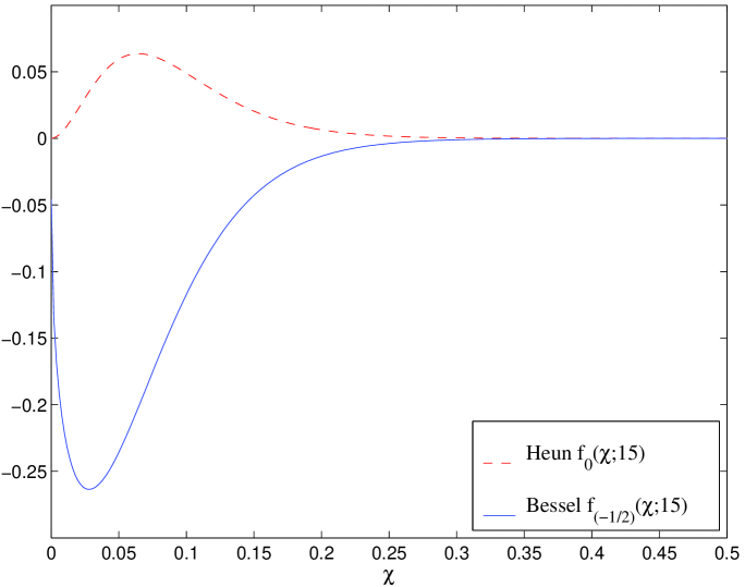
Figure 32. Cut profiles for lowest–order kernels. Here we plot the (positive) Heun profile $f_{0}(\chi;15)$ and the (negative) Bessel profile $f_{(-1/2)}(\chi;15)$, both for $\rho_{B}=15$. To generate both we have used the one–component path method described in Section 2.1.3. The Bessel fdrk $\hat{\omega}_{(-1/2)}(\sigma;15)$ associated with $f_{(-1/2)}(\chi;15)$ is relevant for wave propagation in flat 2+1 dimensional spacetime.

Before turning to a description of the algorithm, let us first give a quick overview of our results. In Table 5 we list the required number $d$ of poles $\beta_{n}$ in (99) corresponding to $\rho_{B}=15$ and two choices of the error tolerance $\varepsilon$. We find these pole numbers to suffice for both the $\jmath=0$ and $\jmath=2$ cases. Notice that $d$ and $l$ appear to grow at different rates, indicating increased performance in the large $l$ limit. However, as we here consider only the relatively small bandwidth $0\leq l\leq 64$, we make this observation with some skepticism. We have extended the $\varepsilon=10^{-6}$ side of the table and found that $d=14$ is sufficient for $l=256$. agh have rigorously shown that for Bessel functions and flatspace wave propagation the number of approximating poles scales like

(102) $$d\sim O\big{(}\log\nu\log(1/\varepsilon)+\log^{2}\nu+\nu^{-1}\log^{2}(1/\varepsilon)\big{)}$$

as $\nu=l+1/2\rightarrow\infty$ and $\varepsilon\rightarrow 0^{+}$. While it is beyond our mathematical ability to analytically establish this or similar growth for Heun functions, the growth indicated in Table 5 is not at odds with this result. Compression is also economical for low–order kernels which are dominated by their continuous sectors. Table 5 lists $d=20$ as sufficient for $\varepsilon=10^{-10}$ and $l=0$. A numerical quadrature of the integral appearing in (68) would require considerably more nodes to achieve this tolerance.

As mentioned above, we have set $x=0$ in all cases (so that the least–squares problem is associated with the Im$\sigma$ axis), and in particular we have done so for $l=0$. This is perhaps remarkable in light of the fact that agh found it necessary to choose $x$ nonzero while approximating the zero–order Bessel fdrk, a case for which the estimate (74) is not applicable. We stress that one need only deal with this zero–order Bessel kernel (a circular rather than spherical boundary kernel) while considering wave propagation on flat 2+1 dimensional spacetime. To emphasize the difference between the $l=0$ Heun fdrk and the $\nu=l+1/2=0$ Bessel fdrk, we plot their cut profiles in Fig. 32. Note that for both cases the kernel, as represented by (68), is determined solely by its cut profile. As documented by agh in [18], loss of differentiability at the origin for the Bessel profile precludes a rational approximation of the zero–order Bessel fdrk by the methods described here, that is unless one chooses $x$ positive and non–zero. For a non–zero positive $x$ a more complicate estimate, valid only for finite time, must be used in place of (74) [18]. Fig. 32 suggests that we may work with $x=0$ even for the lowest–order ($l=0$) Heun fdrk.

3.3.2. Linear least–squares problem

To bypass the nonlinearity of the problem (101), we switch to the linear iterative procedure

(103) $${\rm min}_{P^{(k+1)},Q^{(k+1)}}\int^{\infty}_{-\infty}\left|\frac{P^{(k+1)}(x+{\rm i}y)}{Q^{(k)}(x+{\rm i}y)}-\frac{Q^{(k+1)}(x+{\rm i}y)}{Q^{(k)}(x+{\rm i}y)}\,\hat{\omega}(x+{\rm i}y)\right|^{2}{\rm d}y\,,$$

where given $Q^{(k)}(\sigma)$ the task is to find the minimizing polynomials $P^{(k+1)}(\sigma)$ and $Q^{(k+1)}(\sigma)$. To commence the iteration, we need a degree $d$ polynomial $Q^{(0)}(\sigma)$ as an initial guess, and we describe the construction of initial polynomials in the upcoming Section 3.3.3.

Assuming that we have $Q^{(k)}(\sigma)$ at our disposal, let us now discuss the solution to the least–squares problem (103) at the $k$th level. To do so, we introduce the inner product

(104) $$\left\langle h,g\right\rangle_{k}=\int_{-\infty}^{\infty}h(y)\bar{g}(y)m_{k}(y){\rm d}y\,,$$

where $h(y)$ and $g(y)$ are suitable functions and $m_{k}(y)=1/|Q^{(k)}(x+{\rm i}y)|^{2}$ is the $k$th weight function. Claim: Set $\mathcal{P}(y)=P^{(k+1)}(x+{\rm i}y)$, $\mathcal{Q}(y)=Q^{(k+1)}(x+{\rm i}y)$, $\mathcal{W}(y)=\hat{\omega}(x+{\rm i}y)$, and

(105) $$h_{n}(y)=\left\{\begin{array}[]{ll}(x+{\rm i}y)^{n/2-1}&{\rm for}\,\,n=2,4,6,\dots,2d\\ &\\ (x+{\rm i}y)^{(n-1)/2}\,\mathcal{W}(y)&{\rm for}\,\,n=1,3,5,\dots,2d-1.\end{array}\right.$$

Minimization of the integral (103) is equivalent to

(106) $$\left\langle-\mathcal{P}+\mathcal{Q}\mathcal{W},h_{n}\right\rangle_{k}=0$$

for $n=1,\cdots,2d$.

To verify the claim, first introduce the expansions $\mathcal{P}(y)=\sum_{j=0}^{d-1}p_{j}(x+{\rm i}y)^{j}$ and $\mathcal{Q}(y)=\sum_{j=0}^{d}q_{j}(x+{\rm i}y)^{j}$, assuming $q_{d}=1$. Next, consider a small perturbation $\delta p_{m}$ of the $m$th coefficient $p_{m}$. Vanishment of the induced first–order variation of the integral (103) may then be written as

(107) $$\left\langle-\mathcal{P}+\mathcal{Q}\mathcal{W},h_{2m+2}\right\rangle_{k}\overline{\delta p_{m}}+\overline{\left\langle-\mathcal{P}+\mathcal{Q}\mathcal{W},h_{2m+2}\right\rangle_{k}}\delta p_{m}=0.$$

Finally, exploit the freedom that $\delta p_{m}$ can be either real or imaginary, thereby reaching (106) for even $n=2m+2$. Eq. (106) for odd $n$ follows similarly upon introduction of $\delta q_{m}$ perturbations. $\Box$

With the claim (106) in mind, we orthogonalize the $2d+1$ functions

$$\mathcal{W}(y),\,1,\,(x+{\rm i}y)\mathcal{W}(y),\,(x+{\rm i}y),\,\dots\,,$$

$$(x+{\rm i}y)^{d-1}\mathcal{W}(y),\,(x+{\rm i}y)^{d-1},\,(x+{\rm i}y)^{d}\mathcal{W}(y)\,.$$

The result is a family $\{g_{n}(y):n=1,\dots,2d+1\}$ of orthogonal functions, with the last member $g_{2d+1}(y)$ the sought for solution $-\mathcal{P}(y)+\mathcal{Q}(y)\mathcal{W}(y)$ in (106). We iteratively compute the functions in this family via the formulae

(109) $$g_{n}(y)=\left\{\begin{array}[]{ll}\mathcal{W}(y)&{\rm for}\,\,n=1\\ &\\ 1-c_{21}\mathcal{W}(y)&{\rm for}\,\,n=2\\ &\\ (x+{\rm i}y)g_{n-2}(y)-\sum_{j=1}^{{\rm min}\{4,n-1\}}c_{nj}g_{n-j}(y)&\begin{array}[]{l}{\rm for}\,\,n=3,\\ \dots,2d+1\,,\end{array}\end{array}\right.$$

where the real constants $c_{nj}$ are given by

(110) $$c_{nj}=\left\{\begin{array}[]{ll}\displaystyle\frac{\left\langle 1,\mathcal{W}\right\rangle_{k}}{\left\langle\mathcal{W},\mathcal{W}\right\rangle_{k}}&{\rm for}\,\,n=2\,\,{\rm and}\,\,j=1\\ &\\ \displaystyle\frac{\left\langle(\sigma g_{n-2}),g_{n-j}\right\rangle_{k}}{\left\langle g_{n-j},g_{n-j}\right\rangle_{k}}&\begin{array}[]{l}{\rm for}\,\,n=3,\dots,2d+1\\ {\rm and}\,\,j=1,\dots,{\rm min}\{4,n-1\}\,.\end{array}\end{array}\right.$$

Here we use the notation $(\sigma g_{n-2})(y)$ for the function $(x+{\rm i}y)g_{n-2}(y)$.

A few key observations confirm the correctness of these formulae. As suggested in Figure 18 of Section 2.2.4, the profiles Re$\hat{\omega}({\rm i}y)$ and Im$\hat{\omega}({\rm i}y)$ are of even and odd $y$–parity respectively, and for fixed $x\geq 0$ the profiles Re$\hat{\omega}(x+{\rm i}y)$ and Im$\hat{\omega}(x+{\rm i}y)$ also have the same $y$–parity. Therefore, along the path of integration used to define the inner product, $\mathcal{W}(y)$ has the form $\mathcal{W}^{+}(y)+{\rm i}\mathcal{W}^{-}(y)$, where $\mathcal{W}^{+}$ is even and $\mathcal{W}^{-}$ is odd. Since $x+{\rm i}y$ is also of this form, it follows that all of the functions appearing in the list (LABEL:listoffs) are as well. Now, the integration measure $m_{k}(y)$ appearing in the inner product $\langle\,,\rangle_{k}$ is of even $y$–parity, showing that $\langle\,,\rangle_{k}$ is real–valued on the space (LABEL:listoffs). Whence the $c_{nj}$ are purely real. To see that $c_{nj}=0$ for $j>4$, first suppose that we have carried out the orthogonalization up to the function $g_{n-2}(y)$. In other words, we have $g_{n-2}(y)$ orthogonal to $g_{n-3}(y)$, $g_{n-4}(y)$, $\dots,g_{1}(y)$. Owing to the pattern in the list (LABEL:listoffs), multiplication of $g_{n-2}(y)$ by $x+{\rm i}y$ yields a new function $(\sigma g_{n-2})(y)$ which is not in the span of $g_{n-2}(y)$,$g_{n-3}(y)$, $\dots,g_{1}(y)$. Moreover, $(\sigma g_{n-2})(y)$ is automatically orthogonal to $g_{n-j}(y)$ for $j>4$. Indeed, consider the identity

(111) $$(x+{\rm i}y)g_{n-2}(y)\overline{g}_{n-j}(y)=g_{n-2}(y)\overline{[2xg_{n-j}(y)-(x+{\rm i}y)g_{n-j}(y)]}$$

which implies that

(112) $$\big{\langle}(\sigma g_{n-2}),g_{n-j}\big{\rangle}_{k}=2x\big{\langle}g_{n-2},g_{n-j}\big{\rangle}_{k}-\big{\langle}g_{n-2},(\sigma g_{n-j})\big{\rangle}_{k}\,.$$

Again owing to the pattern in the list (LABEL:listoffs), the function $(\sigma g_{n-j})(y)=(x+{\rm i}y)g_{n-j}(y)$ is in the span of $g_{n+2-j}(y)$, $g_{n+1-j}(y)$, $\dots,g_{1}(y)$. Whence for $j>4$ we see that both terms on the rhs of the last equation vanish, giving $c_{nj}=0$.

3.3.3. Numerical least–squares problem

We sketch how we have handled three issues which arise in numerically implementing the least–squares solve.

Numerical quadrature. To handle the integration necessary to solve (103) via the described orthogonalization, we may change variables and write

(113) $$\int^{\infty}_{-\infty}h(y){\rm d}y=\int^{\pi/2}_{-\pi/2}h(\tan\theta)\sec^{2}\theta{\rm d}\theta\,,$$

where $h(y)$ represents any relevant integrand. This integral is numerically approximated as

(114) $$\sum_{i=0}^{i_{\mathrm{max}}}\lambda_{i}h(\tan\theta_{i})\sec^{2}\theta_{i}\,,$$

where the $\theta_{i}$ and $\lambda_{i}$ are appropriate quadrature nodes and weights.Due to the sum–of–poles form of the fdrk, all encountered integrands $h(\tan\theta)$ are periodic on $[-\pi/2,\pi/2]$. Moreover, all integrands are infinitely continuously differentiable, save possibly at $\theta=0$. By analogy with integer–order Bessel functions, we expect regularity at $\theta=0$ of order $2l+1$ [18]. Whence for high $l$ the trapezoid rule is effective and highly convergent. For low $l$ the profiles Re$\hat{\omega}({\rm i}y)$ and Im$\hat{\omega}({\rm i}y)$ are concentrated around and less regular at the $y$–origin. Therefore, for the first few $l$ we employ an adaptive trapezoid quadrature rule, introducing more nodes around the origin.

Evaluation of $P(\sigma)$, $Q(\sigma)$, and their derivatives. Assume that we have produced a set of real constants $\{c_{nj}:n=2,\dots,2d+1;\,1\leq j\leq 4\}$ belonging to the $k$th linear least–squares problem (103) described in Section 3.3.2. Further, assume that the solution polynomials $P^{(k+1)}(\sigma)$ and $Q^{(k+1)}(\sigma)$ are (close enough to) the polynomials $P(\sigma)$ and $Q(\sigma)$ solving (101). In other words, assume that the iteration in $k$ has converged in some sense. In order to express the final approximating rational function as a pole sum (99), we must first know how to evaluate these polynomials and their derivatives at any $\sigma$ using only the $c_{nj}$ constants. This may be done via the following algorithm. Let $A_{1}=0$, $B_{1}=1$, $A_{2}=-1$, $B_{2}=-c_{21}$, $C_{1}=0$, $D_{1}=0$, $C_{2}=0$, and $D_{2}=0$. Next, for $n=3$ until $2d+1$, set

(115) $$A_{n}=\sigma A_{n-2}-\sum_{j=1}^{4}c_{nj}A_{n-j}\,, C_{n}=A_{n-2}+\sigma C_{n-2}-\sum_{j=1}^{4}c_{nj}C_{n-j}\,,$$

$$B_{n}=\sigma B_{n-2}-\sum_{j=1}^{4}c_{nj}B_{n-j}\,, D_{n}=B_{n-2}+\sigma D_{n-2}-\sum_{j=1}^{4}c_{nj}D_{n-j}\,.$$

Then $P(\sigma)=A_{2d+1}$, $Q(\sigma)=B_{2d+1}$, $P^{\prime}(\sigma)=C_{2d+1}$, $Q^{\prime}(\sigma)=D_{2d+1}$. With the ability to evaluate $Q(\sigma)$ and $Q^{\prime}(\sigma)$ in hand, we may use Newton’s method to obtain the zeros $\beta_{n}$ of $Q(\sigma)$ which are also the pole locations appearing in (99). The corresponding pole strengths are then $\gamma_{n}=P(\beta_{n})/Q^{\prime}(\beta_{n})$.

Construction of the initial guess $Q^{(0)}(\sigma)$. Recall that our sum–of–poles representation of the fdrk features both a discrete sector and a continuous sector. With this in mind, we consider the following two cases.

1. $d\geq N_{l}$. The number of approximating poles is equal to or greater than the number of actual poles from the discrete sector. Therefore, one approximating pole should correspond to each discrete–sector pole. Unless $d=N_{l}$, after each discrete–sector pole has been thusly represented, some approximating poles will be “left over.” These should be placed on the negative Re$\sigma$ axis in order to mimic poles from the continuous sector (cut contribution). In case (i) we aim to naively mimic the actual pole locations found in the exact sum–of–poles representation.

2. $d<N_{l}$. The number of approximating poles is strictly less than number actual poles in the discrete sector, and we do not attempt to naively mimic the pole locations found in the exact sum–of–poles representation.

For case (i) we set $Q^{(0)}(\sigma)=(\sigma-\varsigma_{1})(\sigma-\varsigma_{2})\cdots(\sigma-\varsigma_{d})$. Then for all $i\leq N_{l}$ we let $\varsigma_{i}=15\sigma_{l,i}(15)/\rho_{B}$, that is we set $\varsigma_{i}$ equal to the (numerically obtained) $i$th zero of $W_{l}(15\sigma;\sigma)$ times the ratio $15/\rho_{B}$ (we are also suppressing the $l$ which could be on the $\varsigma_{i}$). If there are any, the remaining $d-N_{l}$ locations $\varsigma_{i}$ are chosen as follows. For each relevant $l$ (in practice for $l\leq 10$) we choose a fixed interval $[a,b]\subset\mathbb{R}_{\leq 0}$ lying on the negative Re$\sigma$ axis. This interval is “eyeballed” to ensure that $[-b,-a]$ includes the essential support of the profile function $f_{l}(\chi;15)$. We then send $a\mapsto 15a/\rho_{B}$ and $b\mapsto 15b/\rho_{B}$. If $d=N_{l}+1$, we let $\varsigma_{d}=(a+b)/2$, and otherwise $\varsigma_{i}=a+(i-N_{l}-1)(b-a)/(d-N_{l}-1)$ with $i$ running from $N_{l}+1$ to $d$.

For case (ii) we set $z=\sigma\rho_{B}$ and then use the Bessel continued fraction expansion (79). As mentioned there, Lenz’s method may be used to evaluate this continued fraction. This method is described in the appendix of Ref. [60]. Via slight modification it may also be used to return a partial denominator, which we use for the value $Q^{(0)}({\rm i}y)$. Indeed, even the most basic algorithm (see Ref. [66]) to compute continued fractions yields a partial denominator and may be used in this fashion.

4. Evolution system and implementation of robc

The goal of this section is to incorporate robc into the MacCormack algorithm, the finite–difference scheme we have used to simulate wave propagation on Schwarzschild blackholes. The first subsection describes the spacetime foliation and associated first–order system of evolution equations on which our numerical work is based. The second reviews the MacCormack algorithm in the context of this system of pde, and it also addresses the issue of inner boundary conditions at the horizon $H$. The third subsection covers implementation of robc. The MacCormack algorithm is a simple, second–order–accurate, predictor–corrector scheme, and we show how robc fit nicely within the framework of the interior prediction and correction. In this final subsection we also touch upon some memory issues relevant to our implementation.

4.1. Spacetime foliation and evolution system

4.1.1. Chosen foliation of spacetime into spacelike slices

Our numerical simulations of wave propagation on the Schwarzschild geometry feature physical coordinates. Moreover, for the time coordinate $t$ and its associated foliation of the spacetime into spacelike slices $\Sigma$ we have chosen one closely related to ingoing Eddington–Finkelstein coordinates. The letter $\Sigma$ is used both to denote the spacetime foliation and a generic slice of the foliation. There are several motivations for switching from the time $T$ (introduced in Section 1.1.1) to $t$ (defined in a moment). Besides removing the coordinate degeneracy present in the diagonal line–element (14), use of the time coordinate $t$ also makes the inner boundary conditions at $H$ particularly easy to set. Although we need not say more to motivate the upcoming discussion, further explanation may be found in Appendix C of [1].

Let us introduce the ingoing Eddington–Finkelstein coordinate system, here in terms of physical rather than dimensionless coordinates. We first pass to physical coordinates by multiplying (14) by an overall factor of $4\mathrm{m}^{2}$ and subsequently sending $4\mathrm{m}^{2}\mathrm{d}s^{2}\mapsto\mathrm{d}s^{2}$. Next, we introduce the physical tortoise coordinate

(116) $$r_{*}=r+2\mathrm{m}\log\big{[}r/(2\mathrm{m})-1\big{]}\,,$$

thereby reaching

(117) $$\mathrm{d}s^{2}=F(-\mathrm{d}T^{2}+\mathrm{d}r_{*}^{2})+r^{2}\mathrm{d}\theta^{2}+r^{2}\sin^{2}\theta\mathrm{d}\phi^{2}\,,$$

where again $F(r)=1-2\mathrm{m}/r$. Using the physical advanced time $v=2\mathrm{m}\nu=T+r_{*}$, we get the line–element in advanced Eddington–Finkelstein form,

(118) $$\mathrm{d}s^{2}=-F\mathrm{d}v^{2}+2\mathrm{d}v\mathrm{d}r+r^{2}\mathrm{d}\theta^{2}+r^{2}\sin^{2}\theta\mathrm{d}\phi^{2}\,.$$

Like the retarded time discussed in Section 1.1.1, the advanced time $v$ also labels characteristic surfaces, but ones which are ingoing (cones which open up towards the past). From a numerical standpoint, we do not want to work directly with a null coordinate like $v$, rather a time coordinate $T_{v}$ obeying $v=T_{v}+r$. Since by definition

(119) $$v=(T+r_{*}-r)+r\,,$$

the desired coordinate is

(120) $$T_{v}=T+r_{*}-r=T+2\mathrm{m}\log\big{[}r/(2\mathrm{m})-1\big{]}\,,$$

and we refer to $T_{v}=v-r$ as ingoing Eddington–Finkelstein time, although as indicated above it is the combination $T_{v}+r$ which labels ingoing characteristics. Likewise, we could introduce a time $T_{u}=u+r$ based on the physical retarded time $u=2\mathrm{m}\mu=T-r_{*}$, but such a time variable would be less suitable for numerical work (see Appendix C of [1]). Let lowercase $t$ represent ingoing Eddington–Finkelstein time shifted by a constant as follows:

(121) $$t=T_{v}-2\mathrm{m}\log\big{[}r_{B}/(2\mathrm{m})-1\big{]}=T+2\mathrm{m}\log\left[\frac{r-2\mathrm{m}}{r_{B}-2\mathrm{m}}\right]\,.$$

The family of level–$t$ slices is the same as the family of level–$T_{v}$ slices, and the combination $t+r$ also labels ingoing characteristics. However, the $t$ coordinate has been tailored to ensure that $t=T$ at the outer boundary $r=r_{B}$.

By construction

(122) $$\mathrm{d}v=\mathrm{d}T_{v}+\mathrm{d}r=\mathrm{d}t+\mathrm{d}r\,,$$

and using this differential relationship, we rewrite (118) as follows:

(123) $$\mathrm{d}s^{2} =-F\mathrm{d}t^{2}+2(1-F)\mathrm{d}t\mathrm{d}r+(2-F)\mathrm{d}r^{2}+r^{2}\mathrm{d}\theta^{2}+r^{2}\sin^{2}\theta\mathrm{d}\phi^{2}$$

$$=-\left[\frac{1}{2-F}\right]\mathrm{d}t^{2}+(2-F)\left[\mathrm{d}r+\frac{(1-F)}{2-F}\mathrm{d}t\right]^{2}+r^{2}\mathrm{d}\theta^{2}+r^{2}\sin^{2}\theta\mathrm{d}\phi^{2}\,.$$

The last line can be written

(124) $$\mathrm{d}s^{2}=-N^{2}\mathrm{d}t^{2}+M^{2}(\mathrm{d}r+V^{r}\mathrm{d}t)^{2}+r^{2}\mathrm{d}\theta^{2}+r^{2}\sin^{2}\theta\mathrm{d}\phi^{2}\,,$$

where the temporal lapse, radial lapse, and shift vector are the following:

(125) $$N(r) =(1+2\mathrm{m}/r)^{-1/2}\,,$$

$$M(r) =(1+2\mathrm{m}/r)^{1/2}\,,$$

$$V^{r}(r) =2\mathrm{m}/(2\mathrm{m}+r)\,.$$

In [27] York discusses the geometric interpretations of such variables in a general setting. For now, the main point is that the line–element (124) is nondegenerate at the horizon $H$, since $N$, $M$, and $V^{r}$ are all well–behaved at $r=2\mathrm{m}$.

4.1.2. Wave equation with respect to chosen foliation

Let us derive the form of the wave equation in the Eddington–Finkelstein system $(t,r,\theta,\phi)$ of coordinates. This can be achieved via coordinate transformation at the level of pde, or by constructing the d’Alembertian associated with (124). Choosing the first method, we start by rewriting (21) in terms of physical coordinates, in order to reach

(126) $$\left(1-\frac{2\mathrm{m}}{r}\right)^{-1}\frac{\partial^{2}\psi_{l}}{\partial T^{2}}-\frac{1}{r^{2}}\frac{\partial}{\partial r}\left[r^{2}\left(1-\frac{2\mathrm{m}}{r}\right)\frac{\partial\psi_{l}}{\partial r}\right]+\frac{l(l+1)\psi_{l}}{r^{2}}-\frac{2\mathrm{m}\jmath^{2}\psi_{l}}{r^{3}}=0\,.$$

In performing the near trivial coordinate transformation $(\tau,\rho)=(\tau(T),\rho(r))$, we have retained the symbol $\psi_{l}$ to denote the new function satisfying the slightly new form (126) of the pde. Next, we introduce the function $U(t,r)=\psi_{l}(T(t),r)$, suppressing from here on out the subscript $l$ which should be on $U$. Then, upon carrying out the coordinate transformation $(T,r)=(T(t),r)$ on (126), we find

$$\left(1+\frac{2\mathrm{m}}{r}\right)\frac{\partial^{2}U}{\partial t^{2}}-\frac{4\mathrm{m}}{r}\frac{\partial^{2}U}{\partial t\partial r}-\left(1-\frac{2\mathrm{m}}{r}\right)\frac{\partial^{2}U}{\partial r^{2}}$$

$$-\frac{2\mathrm{m}}{r^{2}}\frac{\partial U}{\partial t}+\frac{2(\mathrm{m-r)}}{r^{2}}\frac{\partial U}{\partial r}+\frac{l(l+1)U}{r^{2}}-\frac{2\mathrm{m}\jmath^{2}U}{r^{3}}=0$$

for the new form of the wave equation. Upon formal Laplace transformation on $t$, from this equation one recovers Leaver’s normal form for the generalized spheroidal wave equation [44]. In order to trade this second–order equation for a first–order system of equations, we introduce an outgoing characteristic derivative of $U$.

4.1.3. Outgoing characteristic derivative

Construction of the characteristic derivative is based on an understanding of the relevant normal vector fields associated with the $\Sigma$ foliation. Respectively, the following unit vector fields

(128) $$e_{\bot}=N^{-1}\big{(}\partial/\partial t-V^{r}\partial/\partial r\big{)}\,,\qquad e_{\vdash}=M^{-1}\partial/\partial r$$

are the future–pointing normal to the $\Sigma$ foliation and the outward–pointing normal to concentric spheres within a given $\Sigma$ slice [27]. These vectors are depicted in Fig. 33.

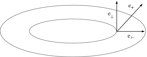
Figure 33. Concentric spheres in a $\Sigma$ slice. The figure depicts two concentric spheres in a single level–$t$ slice as well as the vectors discussed in the text. The $\Sigma$ normal $e_{\bot}$ points out of the slice into the future, while $e_{\vdash}$ points tangent to the slice but normal to the round sphere. These arrows may be extended as vector fields over the whole exterior region.

With normal vector fields (128), we introduce $e_{+}=e_{\bot}+e_{\vdash}$ which is also depicted in Fig. 33. Then $X=e_{+}[U]$ is the characteristic derivative we seek, where $[\;]$ denotes the standard operation of a vector field on a scalar function. More explicitly,

(129) $$X=\frac{1}{N}\frac{\partial U}{\partial t}+\left(\frac{1}{M}-\frac{V^{r}}{N}\right)\frac{\partial U}{\partial r}\,.$$

We now take $(U,X)$ as our basic variables. Since $U$ and $X$ belong to a single spherical–harmonic mode, both should carry $l$ and $m$ subscripts, but we continue to suppress these.

4.1.4. First–order system of evolution equations

To facilitate numerical implementation, we write (LABEL:waveeqnEFin) in a first–order form. The evolution equation for $U$,

(130) $$\partial_{t}U=(V^{r}-M^{-1}N)\partial_{r}U+NX\,,$$

is just the definition (129) of $X$. Eq. (LABEL:waveeqnEFin) now becomes the evolution equation for $X$. We write this equation in the general form

(131) $$\partial_{t}X= (V^{r}+M^{-1}N)\partial_{r}X-N\big{(}X^{M}_{-}+2X^{R}_{+}\big{)}X+R^{2}X\partial_{r}\alpha$$

$$+2M^{-1}NX^{R}_{+}\partial_{r}U-R^{-2}Nl(l+1)U+2\mathrm{m}NR^{-3}\jmath^{2}U\,,$$

where $R$ is the areal radius, $X^{M}_{-}$ and $X^{R}_{+}$ are certain characteristic variables of the background geometry, and $\alpha=N/(MR^{2})$ is the “dedensitized lapse.” In this general notation one might denote our main characteristic variable (129) by $X^{U}_{+}$ rather than plain $X$, but there is no need to do so here. In terms of the round–sphere area $A$, the variable $R$ is defined geometrically as $[A/(4\pi)]^{1/2}$, and, therefore, $R=r$ for the Eddington–Finkelstein system. Moreover, in terms of the “Einstein–Christoffel variables” $K_{M}$, $K_{R}$, $f_{M}$ and $f_{R}$ written in Eqs. (2.2) and (2.3) of Ref. [33], we have $X^{M}_{-}=-K_{M}-f_{M}$ and $X^{R}_{+}=-K_{R}+f_{R}$. For the evolution at hand all of these variables are fixed, and in the numerical implementation they amount to function calls given by

(132) $$R(r) =r\,,$$

(133) $$\partial_{r}\alpha(r) =-\frac{2(\mathrm{m}+r)}{(2\mathrm{m}r+r^{2})^{2}}\,,$$

(134) $$X^{R}_{+}(r) =\frac{r-2\mathrm{m}}{2\mathrm{m}r+r^{2}}\left[1+\frac{2\mathrm{m}}{r}\right]^{1/2}\,,$$

(135) $$X^{M}_{-}(r) =\frac{2\mathrm{m}^{2}-5\mathrm{m}r-4r^{2}}{r(2\mathrm{m}+r)^{2}}\left[1+\frac{2\mathrm{m}}{r}\right]^{1/2}\,.$$

We remark that the variable $X^{R}_{+}=e_{+}[\log R]$, whence describes the rate of change of the logarithm of areal radius along the outgoing null direction. Note that $X^{R}_{+}(2\mathrm{m})=0$. Despite the somewhat general form (131) we have chosen for the wave equation, it is nothing but a tedious exercise in elementary algebra to substitute the given expressions for $X$, $N$, $M$, $V^{r}$, $R$, $X^{M}_{-}$, $X^{R}_{+}$, and $\partial_{r}\alpha$ into (131) in order to recover ($N$ times) Eq. (LABEL:waveeqnEFin). In performing this exercise, note right away that

(136) $$V^{r}+M^{-1}N=1$$

for the chosen coordinate system. Each of the evolution equations (130,131) has the form of a forced advection equation, and in particular we can write (131) as follows:

(137) $$\partial_{t}X=\partial_{r}X+S(r,X,U,\partial_{r}U)\,,$$

where the source term $S$ is defined by comparison of this equation with (131). Note that $S$ also depends on the parameters $l$, $\jmath$, and $\mathrm{m}$.

4.2. Interior of the computational domain and horizon: numerical details

4.2.1. MacCormack predictor–corrector scheme

Suppose that the radial mesh is the collection of $Q+1$ nodes $r_{q}$, where $r_{0}=2\mathrm{m}$, $r_{Q}=r_{B}=2\mathrm{m}\rho_{B}$, and $r_{q}=2\mathrm{m}+q\Delta r$. The spatial discretization step is $\Delta r=(r_{B}-2\mathrm{m})/Q$. Once the number $Q$ of spatial subintervals is fixed, the temporal discretization step $\Delta t$ is determined by fixing the Courant number $\Delta t/\Delta r$. Let the temporal mesh nodes be $t_{n}=n\Delta t$, and define, for example, the mesh function $U^{n}_{q}=U(t_{n},r_{q})$. To simplify the presentation, our analysis holds $U^{n}_{q}$ as the exact value of $U(t,r)$ at $(t_{n},r_{q})$. Our task of numerical evolution on the interior of the computational domain is then to produce approximations, $\widetilde{U}^{n+1}_{q}$ and $\widetilde{X}^{n+1}_{q}$, to the true values $U^{n+1}_{q}$ and $X^{n+1}_{q}$ (doing so for $0<q<Q$), given in advance both $U^{n}_{q}$ and $X^{n}_{q}$ (for $0\leq q\leq Q$) as well as the exact geometry function calls $N_{q}$, $M_{q}$, $V^{r}_{q}$, $R_{q}$, $[X^{R}_{+}]_{q}$, $[X^{M}_{-}]_{q}$, and $[\partial_{r}\alpha]_{q}$ listed in Eqs. (125,132–135). Here, for example, $M_{q}=M(r_{q})$ and $[X^{M}_{-}]_{q}=X^{M}_{-}(r_{q})$. As these functions calls are time–independent, they need not carry the time superscript $n$. We choose the MacCormack scheme to accomplish our task. This scheme is in consistent conservation form [45] as applied to a conservation law like the $1+1$ scalar wave equation. Since our primary focus is numerical implementation of robc, it pays to keep the interior evolution simple in order to highlight the implementation.

Let us quickly review the MacCormack scheme in the context of the variables at hand. First consider the following predicted variables which stem from straightforward differencing of (130,137):

(138) $$\bar{U}^{n+1}_{q} =U^{n}_{q}+\Delta t\big{[}\,(V^{r}-M^{-1}N)_{q}\,D_{-}U^{n}_{q}+N_{q}\,X^{n}_{q}\big{]}\,,$$

$$\bar{X}^{n+1}_{q} =X^{n}_{q}+\Delta t\big{[}D_{+}X^{n}_{q}+S^{n}_{q}\big{]}\,.$$

Here $D_{\mp}$ denotes either a downwind or upwind difference stencil,

(139) $$D_{-}U^{n}_{q}=\big{(}U^{n}_{q}-U^{n}_{q-1}\big{)}\big{/}\Delta r\,,\quad D_{+}X^{n}_{q}=\big{(}X^{n}_{q+1}-X^{n}_{q}\big{)}\big{/}\Delta r\,.$$

To approximate the $\partial_{r}U$ appearing in the $S^{n}_{q}$ source in the second equation of (138), we use a centered difference stencil. The predicted variables $\bar{U}^{n+1}_{q}$ and $\bar{X}^{n+1}_{q}$ are not second–order–accurate approximations to the values $U^{n+1}_{q}$ and $X^{n+1}_{q}$ in question. However, the corrected variables

(140) $$\widetilde{U}^{n+1}_{q} =0.5\big{\{}\bar{U}^{n+1}_{q}+U^{n}_{q}+\Delta t\big{[}(V^{r}-M^{-1}N)_{q}\,D_{+}\bar{U}^{n+1}_{q}+N_{q}\,\bar{X}{}^{n+1}_{q}\big{]}\big{\}}\,,$$

$$\widetilde{X}^{n+1}_{q} =0.5\big{\{}\bar{X}^{n+1}_{q}+X^{n}_{q}+\Delta t\big{[}D_{-}\bar{X}^{n+1}_{q}+\bar{S}{}^{n+1}_{q}\big{]}\big{\}}\,,$$

are indeed second–order–accurate approximations. To approximate the advection derivative term in the correction phase (140), we have incorporated stencils $D_{\pm}$ opposite to those $D_{\mp}$ used for the same term in the prediction phase (138). The source term $\bar{S}{}^{n+1}_{q}$ at the next time step is built both with time–independent function calls and barred variables. We again use a centered stencil to handle the derivative term in the source, but now one

(141) $$\overline{[\partial_{r}U]}{}^{n+1}_{q}=0.5\big{(}\bar{U}^{n+1}_{q+1}-\bar{U}^{n+1}_{q-1}\big{)}\big{/}\Delta r$$

built with predicted values.

4.2.2. Inner boundary conditions at $H$

From (131) or (137) we see that $X$ propagates according to the cartoon $H\nwarrow B$, that is to say inward from $B$ towards $H$, and at unit speed with respect to the coordinate time axis $\partial/\partial t$. Eqs. (132,133,136) then determine the following form for the $X$ evolution equation at the horizon:

$$\big{[}\partial_{t}X-\partial_{r}X\big{]}\big{|}_{r=2\mathrm{m}}=$$

$$-\big{[}NX^{M}_{-}X-r^{2}X\partial_{r}\alpha+r^{-2}Nl(l+1)U-2\mathrm{m}Nr^{-3}\jmath^{2}U\big{]}\big{|}_{r=2\mathrm{m}}\,,$$

Notice the absence of the derivative term involving $\partial_{r}U$ on the rhs. As $X^{R}_{+}(2\mathrm{m})=0$, it has been dropped. Eq. (LABEL:fourdotXatH) shows that $X$ propagates inward at $H$, whence there is no analytical issue of an inner boundary condition for $X$.

The coordinate velocity appearing in (130) is

(143) $$-V^{r}+M^{-1}N=\frac{r-2\mathrm{m}}{r+2\mathrm{m}}\,,$$

and it is monotonically increasing on $[2\mathrm{m},\infty)$ with $0\leq-V^{r}+M^{-1}N<1$. This shows that $U$ propagates according to the cartoon $H\nearrow B$, at least for $r>2\mathrm{m}$. More precisely, $U$ propagates outward at speed $|V^{r}-M^{-1}N|$ with respect to the coordinate time axis $\partial/\partial t$. Furthermore, at the horizon

(144) $$\partial_{t}U\big{|}_{r=2\mathrm{m}}=NX\big{|}_{r=2\mathrm{m}}\,,$$

since $-V^{r}+M^{-1}N$ vanishes for $r=2\mathrm{m}$. Therefore, $U$ propagates straight up the coordinate time axis at $H$, and there is no analytical issue of an inner boundary condition for $U$. Indeed, in tandem with the way (LABEL:fourdotXatH) the variable $X$ propagates, Eq. (144) implies that the region inside of $r=2\mathrm{m}$ has no causal influence (insofar as the disturbances $U$ and $X$ are concerned) on the region outside of $r=2\mathrm{m}$. Heuristically, $H$ acts as a one–way membrane.

As for numerical inner boundary conditions at $H$, we extend the radial mesh past the horizon by adding a ghost node $r_{-1}=2\mathrm{m}-\Delta r$. At both the prediction stage and correction stage, values at the ghost node are obtained via a simple copy–over from its righthand neighbor $r_{0}=2\mathrm{m}$: $\bar{U}{}^{n+1}_{-1}=\bar{U}{}^{n+1}_{0}$, $\bar{X}{}^{n+1}_{-1}=\bar{X}{}^{n+1}_{0}$, $\widetilde{U}{}^{n+1}_{-1}=\widetilde{U}{}^{n+1}_{0}$, and $\widetilde{X}{}^{n+1}_{-1}=\widetilde{X}{}^{n+1}_{0}$. Of course, these are not the correct inner boundary conditions, but any resulting numerical error is trapped within the region $r<2\mathrm{m}$ as shown by careful examination of the outlined MacCormack difference scheme at the point $r_{0}=2\mathrm{m}$. Indeed, owing to the aforementioned identity $[X^{+}_{R}]_{0}=0$ which kills the $\partial_{r}U$ term in (131), the predicted variable $\bar{X}{}^{n+1}_{0}$ depends neither on $U^{n}_{-1}$ nor $X^{n}_{-1}$. Likewise, since $(V^{r}-M^{-1}N)_{0}=0$, the predicted variable $\bar{U}{}^{n+1}_{0}$ also depends neither on $U^{n}_{-1}$ nor $X^{n}_{-1}$. Next, because $\bar{X}{}^{n+1}_{-1}$ is a copy–over of $\bar{X}{}^{n+1}_{0}$ (so that $D_{-}\bar{X}{}^{n+1}_{0}=0$ holds), the corrected variable $\widetilde{X}{}^{n+1}_{0}$ does not depend on mesh values at $r_{-1}$. Therefore, we see that $\widetilde{U}{}^{n+1}_{0}$ also does not depend on values at $r_{-1}$, in parallel with the fact that physically the region $r<2\mathrm{m}$ cannot influence $H$.

4.3. Implementation of robc

4.3.1. robc in physical coordinates

We may rewrite the convolution (62) in terms of the physical coordinates via division of the equation by an overall factor of $2\mathrm{m}$. The result is

(145) $${\sf X}_{l}(T,r_{B})+\frac{\psi_{l}(T,r_{B})}{{\sf M}(r_{B})r_{B}}=r_{B}^{-1}{\sf N}(r_{B})\int^{T}_{0}\Omega_{l}(T-T^{\prime};r_{B})\psi_{l}(T^{\prime},r_{B})\mathrm{d}T^{\prime}\,,$$

where we have defined the physical tdrk

(146) $$\Omega_{l}(T;r_{B})=\frac{\omega_{l}(T/(2\mathrm{m});r_{B}/(2\mathrm{m}))}{2\mathrm{m}}\,.$$

Also appearing in (145) is

(147) $${\sf X}_{l}=\frac{1}{{\sf N}}\frac{\partial\psi_{l}}{\partial T}+\frac{1}{{\sf M}}\frac{\partial\psi_{l}}{\partial r}\,,$$

the characteristic derivative ${\sf e}_{+}[\psi_{l}]$ of $\psi_{l}$ along a null direction ${\sf e}_{+}$ which points outward and towards the future.

We note that the null vector

(148) $${\sf e}_{+}=\frac{1}{{\sf N}}\frac{\partial}{\partial T}+\frac{1}{{\sf M}}\frac{\partial}{\partial r}$$

points in the same direction as the one

(149) $$e_{+}=\frac{1}{N}\frac{\partial}{\partial t}+\left(\frac{1}{M}-\frac{V^{r}}{N}\right)\frac{\partial}{\partial r}$$

considered earlier. However, they have different extents and are related by a pure boost,

(150) $${\sf e}_{+}=e^{\vartheta}e_{+}\,,$$

through a hyperbolic angle

(151) $$\vartheta={\textstyle\frac{1}{2}}\log\left[\frac{1+N^{-1}MV^{r}}{1-N^{-1}MV^{r}}\right]\,.$$

Since the proper spatial velocity $MV^{r}/N=2\mathrm{m}/r<1$ for $r>2\mathrm{m}$, the argument of the logarithm is positive on the exterior region.

4.3.2. robc in Eddington–Finkelstein coordinates

The physical convolution (145) is expressed with respect to spacelike slices which are level in the static time variable $T$. We now wish to express the convolution (145) with respect to the spacelike slices $\Sigma$ which are level in the ingoing Eddington-Finkelstein time $t$. Since we have arrange for $T=t$ at the outer boundary $r=r_{B}$, we may express the physical robc given in (145) as follows:

(152) $$e^{\vartheta_{B}}X(t,r_{B})+\frac{U(t,r_{B})}{{\sf M}(r_{B})r_{B}}=r_{B}^{-1}{\sf N}(r_{B})\int^{t}_{0}\Omega(t-t^{\prime};r_{B})U(t^{\prime},r_{B})\mathrm{d}t^{\prime}\,.$$

To reach this equation, drop the $l$ subscript on $\Omega_{l}$, enact a trivial change of variables, and appeal to the equalities

(153) $${\sf X}_{l}={\sf e}_{+}[\psi_{l}]=e^{\vartheta}e_{+}[U]=e^{\vartheta}X\,.$$

The middle equality stems from (150), and it of course holds at the outer boundary where we use the shorthand $\vartheta_{B}=\vartheta(r_{B})$. In this middle equality we have also dropped the subscript $l$. In (152) we have chosen to retain ${\sf N}(r_{B})$ and ${\sf M}(r_{B})$, although they could be traded for $N(r_{B})$ and $M(r_{B})$ at the expense of introducing further boost factors. In any case, they are simply fixed constants, insofar as the robc are concerned.

4.3.3. Approximate time–domain radiation kernel

From now until the end of this subsection we reinstate the policy of suppressing all factors of $l$. Moreover, for the most part we also suppress factors of $\rho_{B}$, or $r_{B}$ as the case may be. The technique of kernel compression discussed in Section 3.3 yields an approximate fdrk $\hat{\xi}(\sigma)=P(\sigma)/Q(\sigma)$ of the form (99). The inverse Laplace transform $\mathcal{L}^{-1}[\hat{\xi}](\tau)$ of this approximate fdrk is an approximate tdrk

(154) $$\xi(\tau)=\sum_{n=1}^{d}\gamma_{n}\exp(\beta_{n}\tau)\,.$$

Note that the $d$ pole locations $\beta_{n}=\beta^{R}_{n}+\mathrm{i}\beta^{I}_{n}$ and strengths $\gamma_{n}=\gamma^{R}_{n}+\mathrm{i}\gamma^{I}_{n}$ are generally complex and the locations (are numerically observed to) lie in the lefthalf plane. In order to pass to a physical approximate tdrk $\Xi(t)=\xi(t/(2\mathrm{m}))/(2\mathrm{m})$, we set $\beta_{n}=2\mathrm{m}b_{n}$ and $\gamma_{n}=2\mathrm{m}c_{n}$, thereby reaching

(155) $$\Xi(t)=\sum_{n=1}^{d}c_{n}\exp(b_{n}t)\,.$$

We list a representative set of pole locations and strengths in Table 6. Note that these must be scaled for use in the physical kernel. For $\rho_{B}=15$ as in the table and a blackhole of mass $\mathrm{m}=2$, we would obtain the pole locations $b_{n}$ and strengths $c_{n}$ corresponding to $r_{B}=60$ upon dividing the entries in the table by $4=2\mathrm{m}$.

$\beta^{R}_{1}+\mathrm{i}\beta^{I}_{1}$	$-0.20807160+\mathrm{i}0$
$\beta^{R}_{2}+\mathrm{i}\beta^{I}_{2}$	$-0.18971337+\mathrm{i}0.06900399$
$\beta^{R}_{3}+\mathrm{i}\beta^{I}_{3}$	$-0.13304751+\mathrm{i}0.17772749$
$\beta^{R}_{4}+\mathrm{i}\beta^{I}_{4}$	$-0.18971337-\mathrm{i}0.06900399$
$\beta^{R}_{5}+\mathrm{i}\beta^{I}_{5}$	$-0.13304751-\mathrm{i}0.17772749$
$\gamma^{R}_{1}+\mathrm{i}\gamma^{I}_{1}$	$-0.07445512+\mathrm{i}0$
$\gamma^{R}_{2}+\mathrm{i}\gamma^{I}_{2}$	$-0.17152322+\mathrm{i}0.07630724$
$\gamma^{R}_{3}+\mathrm{i}\gamma^{I}_{3}$	$-0.12569363+\mathrm{i}0.17804157$
$\gamma^{R}_{4}+\mathrm{i}\gamma^{I}_{4}$	$-0.17152322-\mathrm{i}0.07630724$
$\gamma^{R}_{5}+\mathrm{i}\gamma^{I}_{5}$	$-0.12569363-\mathrm{i}0.17804157$

Table 6. Pole locations and strengths for a compressed kernel. Here the compressed kernel corresponds to $\jmath=0$, $l=4$, $\rho_{B}=15$, and $\varepsilon=10^{-6}$. Note that the number of poles is $d=5$ in accord with Table 5 from Section 3.3.1. Both the $0$ in $\beta_{1}$ and the $0$ in $\gamma_{1}$ correspond to output numbers from the compression algorithm which are of order $10^{-47}$.

Of the $d$ poles $d_{\mathrm{sing}}$ will lie on the negative real axis and there will be $d_{\mathrm{pair}}$ complex–conjugate pairs. So $d=d_{\mathrm{sing}}+2d_{\mathrm{pair}}$ always holds. For the compressed kernel shown in Table 6, we have $d_{\mathrm{sing}}=1$ and $d_{\mathrm{pair}}=2$. We then break up $\Xi(t)$ as follows:

(156) $$\Xi(t)=\sum_{i=1}^{d_{\mathrm{sing}}}H_{i}(t)+\sum_{j=1}^{d_{\mathrm{pair}}}G_{j}(t)\,.$$

In this decomposition

(157) $$H_{i}(t)=\mu_{i}\exp(\kappa_{i}t)\,,\;G_{j}(t)=2\left[m^{R}_{j}\cos(k^{I}_{j}t)-m^{I}_{j}\sin(k^{I}_{j}t)\right]\exp(k^{R}_{j}t)\,,$$

where $\kappa_{i}$ and $\mu_{i}$ respectively correspond to a pole location $b^{R}_{n}+\mathrm{i}0$ and strength $c^{R}_{n}+\mathrm{i}0$ (each lying on the negative real axis), while $k^{R}_{j}+\mathrm{i}k^{I}_{j}$ and $m^{R}_{j}+\mathrm{i}m^{I}_{j}$ respectively correspond to a pole location $b^{R}_{n}+\mathrm{i}b^{I}_{n}$ and strength $c^{R}_{n}+\mathrm{i}c^{I}_{n}$ (each lying properly in the second quadrant). One should not confuse the $k^{R}_{j}+\mathrm{i}k^{I}_{j}$ with the zeros $k_{l,n}$ of the MacDonald function considered in Sections 2.1.3 and 3.1.1. For the compressed kernel considered in Table 6 we list these reordered locations and strengths in Table 7. We also need to consider an auxiliary object,

(158) $$F_{j}(t)=2\left[m^{I}_{j}\cos(k^{I}_{j}t)+m^{R}_{j}\sin(k^{I}_{j}t)\right]\exp(k^{R}_{j}t)\,,$$

not appearing directly in the kernel. We then use

(159) $$(\Xi*U)(t)=\sum_{i=1}^{d_{\mathrm{sing}}}\int^{t}_{0}H_{i}(t-t^{\prime})U(t^{\prime})\mathrm{d}t^{\prime}+\sum_{j=1}^{d_{\mathrm{pair}}}\int^{t}_{0}G_{j}(t-t^{\prime})U(t^{\prime})\mathrm{d}t^{\prime}\,,$$

as an approximation to the convolution $(\Omega*U)(t)$ in (152).

$2\mathrm{m}\kappa_{1}$	$-0.20807160$
$2\mathrm{m}(k^{R}_{1}+\mathrm{i}k^{I}_{1})$	$-0.18971337+\mathrm{i}0.06900399$
$2\mathrm{m}(k^{R}_{2}+\mathrm{i}k^{I}_{2})$	$-0.13304751+\mathrm{i}0.17772749$
$2\mathrm{m}\mu_{1}$	$-0.07445512$
$2\mathrm{m}(m^{R}_{1}+\mathrm{i}m^{I}_{1})$	$-0.17152322+\mathrm{i}0.07630724$
$2\mathrm{m}(m^{R}_{2}+\mathrm{i}m^{I}_{2})$	$-0.12569363+\mathrm{i}0.17804157$

Table 7. Reordered pole locations and strengths for a compressed kernel. Here we show the reordered locations and strengths which render the compressed kernel in Table 6 manifestly real. Compare these numbers with those in Table 6. A choice of mass must be made to determine these values. In this table and the text one should make a distinction between the mass (plain $\mathrm{m}$) and the numerical pole strength $m_{j}$ (italic $m$ and with a subscript).

The update $(\Xi*U)(t+\Delta t)$ plays a central role in our implementation of robc. We write it as follows:

(160) $$(\Xi*U)(t+\Delta t)=\int_{0}^{t}\Xi(t+\Delta t-t^{\prime})U(t^{\prime})\mathrm{d}t^{\prime}+\int_{t}^{t+\Delta t}\Xi(t+\Delta t-t^{\prime})U(t^{\prime})\mathrm{d}t^{\prime}\,,$$

respectively referring to the first and second integrals on the rhs as the history part ${}_{\mathtt{H}}(\Xi*U)(t+\Delta t)$ and the local part ${}_{\mathtt{L}}(\Xi*U)(t+\Delta t)$ of the updated convolution. In the same fashion, $(H_{i}*U)(t+\Delta t)$, $(F_{j}*U)(t+\Delta t)$, and $(G_{j}*U)(t+\Delta t)$ can each be split into history and local parts. Computing the update $(\Xi*U)(t+\Delta t)$ then amounts to computing the history and local parts of both $(G_{j}*U)(t+\Delta t)$ and $(H_{i}*U)(t+\Delta t)$. We discuss the local parts of these convolutions below, but here note that the history parts may be computed via the following exact identities:

(161)

$${}_{\mathtt{H}}(H_{i}*U)(t+\Delta t) =\exp(\kappa_{i}\Delta t)(H_{i}*U)(t)\,,$$

$${}_{\mathtt{H}}(G_{j}*U)(t+\Delta t) =\exp(k^{R}_{j}\Delta t)\big{[}\cos(k^{I}_{j}\Delta t)(G_{j}*U)(t)-\sin(k^{I}_{j}\Delta t)(F_{j}*U)(t)\big{]}\,,$$

$${}_{\mathtt{H}}(F_{j}*U)(t+\Delta t) =\exp(k^{R}_{j}\Delta t)\big{[}\cos(k^{I}_{j}\Delta t)(F_{j}*U)(t)+\sin(k^{I}_{j}\Delta t)(G_{j}*U)(t)\big{]}\,.$$

These follow from elementary exponential and trigonometric identities. The recursive evaluation of the history dependence afforded by identities (161) leads to a considerable reduction in computational storage cost. A direct evaluation of the boundary convolution would require $O(t/\Delta t)$ memory locations to store the whole history of $U$ along the timelike cylinder ${}^{3}\!B$ (see Figure 1 in the introduction). Our algorithm requires only the memory needed to store (the constituent pieces for) $(\Xi*U)^{n}$ as well as the numerical pole strengths and locations ($2d=2d_{\mathrm{sing}}+4d_{\mathrm{pair}}$ real numbers).

4.3.4. Incorporation of robc into predictor–corrector algorithm

At $t=t_{n}$ suppose that we are given (i) $U^{n}_{q}$ and $X^{n}_{q}$ for $0\leq q\leq Q$, (ii) $(\Xi*U)^{n}=(\Xi*U)(t_{n};r_{B})$, and (iii) the necessary procedures to perform interior update as described in Section 4.2.1. For the second assumption, we actually require $\forall i,j$ that $(H_{i}*U)^{n}$, $(G_{j}*U)^{n}$, and $(F_{j}*U)^{n}$ are individually given. Again, for ease of presentation we assume that all of these present time–step expressions are exact. Our implementation of robc then amounts to the following task: use (152) to produce second–order accurate approximations

(162) $$\widetilde{U}^{n+1}_{Q}\,,\quad\widetilde{X}^{n+1}_{Q}\,,\quad\widetilde{(\Xi*U)}{}^{n+1}$$

to the true values $U^{n+1}_{Q}$, $X^{n+1}_{Q}$, and $(\Xi*U)^{n+1}$. The notation $\widetilde{(\Xi*U)}{}^{n+1}$ is shorthand for the pieces

(163) $$\widetilde{(H_{i}*U)}{}^{n+1}\,,\quad\widetilde{(G_{j}*U)}{}^{n+1}\,,\quad\widetilde{(F_{j}*U)}{}^{n+1}\,.$$

We emphasize that $U^{n+1}_{Q}$ and $X^{n+1}_{Q}$ are the true values associated with a field freely radiating on a larger domain.

We accomplish the task using the framework of the interior prediction–correction algorithm. Before entering the prediction phase, let us see what can be precomputed and stored for use during the course of the algorithm. First, we have

(164) $$\Xi(0)=\sum_{i=1}^{d_{\mathrm{sing}}}H_{i}(0)+\sum_{j=1}^{d_{\mathrm{pair}}}G_{j}(0)\,,\qquad\Xi(\Delta t)=\sum_{i=1}^{d_{\mathrm{sing}}}H_{i}(\Delta t)+\sum_{j=1}^{d_{\mathrm{pair}}}G_{j}(\Delta t)$$

at our disposal from $t=t_{0}=0$ onwards. Second, at the time step $t=t_{n}$, we may appeal to the identities (161) in order to exactly calculate and store the history parts ${}_{\mathtt{H}}(H_{i}*U)^{n+1}$, ${}_{\mathtt{H}}(G_{j}*U)^{n+1}$, and ${}_{\mathtt{H}}(F_{j}*U)^{n+1}$ $\forall i,j$. With these we then exactly calculate the history part ${}_{\mathtt{H}}(\Xi*U)^{n+1}$ of the updated total convolution $(\Xi*U)^{n+1}$.

Let us now describe the prediction phase. Due to the way we have chosen the difference stencils in (138), the boundary prediction $\bar{U}^{n+1}_{Q}$ may be calculated from the same formula,

(165) $$\bar{U}^{n+1}_{Q}=U^{n}_{Q}+\Delta t\big{[}(V^{r}-M^{-1}N)_{Q}\,(U^{n}_{Q}-U^{n}_{Q-1})\big{/}\Delta r+N_{Q}\,X^{n}_{Q}\big{]}\,,$$

used in the interior prediction. We then substitute $\bar{U}^{n+1}_{Q}$ into the approximation to (152) obtained by replacing $\Omega$ with $\Xi$, thereby obtaining the “predicted” characteristic variable at the next time step. Namely,

(166) $$\bar{X}^{n+1}_{Q}=r_{B}^{-1}{\sf N}_{B}e^{-\vartheta_{B}}\left[{}_{\mathtt{H}}(\Xi*U)^{n+1}+{}_{\mathtt{L}}\overline{(\Xi*U)}{}^{n+1}-\bar{U}^{n+1}_{Q}\right]\,,$$

where we use the shorthands ${\sf N}_{B}={\sf N}(r_{B})=1/{\sf M}(r_{B})$ and

(167) $${}_{\mathtt{L}}\overline{(\Xi*U)}{}^{n+1}=0.5\Delta t\big{[}\Xi(\Delta t)U^{n}_{Q}+\Xi(0)\bar{U}^{n+1}_{Q}\big{]}\,.$$

The last shorthand ${}_{\mathtt{L}}\overline{(\Xi*U)}{}^{n+1}$ is a prediction for the local part ${}_{\mathtt{L}}(\Xi*U)^{n+1}$ of the updated total convolution $(\Xi*U)^{n+1}$. This prediction is based on trapezoidal approximation of the second integral appearing on the rhs of (160). In Section 5.1.2 we also consider what results from both rectangular and parabolic approximations as well as the trapezoidal approximation at hand.

Turning to the correction phase, we first obtain

(168) $$\widetilde{U}{}^{n+1}_{Q}= 0.5\Big{\{}\bar{U}{}^{n+1}_{Q}+U^{n}_{Q}$$

$$+\Delta t\Big{[}(V^{r}-M^{-1}N)_{Q}\,(\bar{U}{}^{n+1}_{Q+1}-\bar{U}{}^{n+1}_{Q})\big{/}\Delta r+N_{Q}\,\bar{X}{}^{n+1}_{Q}\Big{]}\Big{\}}\,.$$

In this formula $\bar{U}^{n+1}_{Q+1}$ is not available from the prediction phase, whence it is computed via the extrapolation

(169) $$\bar{U}{}^{n+1}_{Q+1}=3\bar{U}{}^{n+1}_{Q}-3\bar{U}{}^{n+1}_{Q-1}+\bar{U}{}^{n+1}_{Q-2}\,.$$

We discuss this detail of our implementation in the Appendix. Next, we compute the “corrected” variable

(170) $$\widetilde{X}{}^{n+1}_{Q}=r_{B}^{-1}{\sf N}_{B}e^{-\vartheta_{B}}\left[{}_{\mathtt{H}}(\Xi*U){}^{n+1}+{}_{\mathtt{L}}\widetilde{(\Xi*U)}{}^{n+1}-\widetilde{U}{}^{n+1}_{Q}\right]\,,$$

where as before

(171) $${}_{\mathtt{L}}\widetilde{(\Xi*U)}{}^{n+1}=0.5\Delta t\big{[}\Xi(\Delta t)U^{n}_{Q}+\Xi(0)\widetilde{U}{}^{n+1}_{Q}\big{]}\,.$$

To end the correction phase, we similarly obtain $\forall i,j$

(172) $${}_{\mathtt{L}}\widetilde{(F_{j}*U)}{}^{n+1}\,,\qquad{}_{\mathtt{L}}\widetilde{(G_{j}*U)}{}^{n+1}\,,\qquad{}_{\mathtt{L}}\widetilde{(H_{i}*U)}{}^{n+1}\,,$$

and use these to update the constituent pieces of the convolution. For example, we take

(173) $$\widetilde{(G_{j}*U)}{}^{n+1}={}_{\mathtt{H}}(G_{j}*U){}^{n+1}+{}_{\mathtt{L}}\widetilde{(G_{j}*U)}{}^{n+1}\,,$$

as the desired approximation to the updated total convolution $(G_{j}*U)^{n+1}$.

5. Numerical tests

This section documents the results of several numerical tests of our implementation of robc. Throughout, we consider a blackhole of mass $\mathrm{m}=2$ enclosed within an outer boundary of radius $r_{B}=60$ so that the horizon is located at $2\mathrm{m}=4$ and $\rho_{B}=15$. For this choice of $r_{B}$ the outer boundary $B$ lies in the weak–field region (see the second paragraph of Section 3). As mentioned in the introduction, we have chosen $\mathrm{m}=2$ only to have an example for which the mass is neither $1$ nor $\frac{1}{2}$. Our numerical tests cover both $\jmath=0,2$ cases as well as various values of $l$. Results carried out with $\rho_{B}=20$ are similar, but not reported. A more detailed investigation of these boundary conditions is forthcoming [67].

5.1. One–dimensional radial evolutions

Tests based on one–dimensional evolutions most effectively examine the issues of convergence and error for our robc, and this subsection is devoted to them. We first examine both issues in the context of a short–time numerical evolution. Subsequently, we further examine the issue of numerical error for our robc by considering two long–time evolutions. We also consider a third long–time evolution, although not in the context of an error analysis.

5.1.1. Short–time evolution

Given fixed values for $l$ and $\jmath$, we have taken the initial data $U(0,r)$ shown in the top plot of Fig. 34. We have set $U(0,r)=f(r)/r$, where

(174) $$f(r)=A\exp\left[\frac{8\delta}{(b-a)^{2}}\right]\left/\exp\left[\frac{\delta}{(r-a)^{2}}+\frac{\delta}{(b-r)^{2}}\right]\right.$$

for $A=50$, $a=45$, $b=55$, and $\delta=20$. The profile $U(0,r)$ is then compactly supported on $[45,55]$ and of $C^{\infty}$ class. We choose $X(0,r)=-U(0,r)/r$ as the other initial condition. The resulting initial data set would be a pure outgoing were we considering $l=0$ and flat Minkowski spacetime. For the case at hand, whatever the fixed values $l$ and $\jmath$ are, the initial data is not purely outgoing but will reach the outer boundary $r_{B}=60$ in a time (about 5) which is short relative to the crossing time of the domain $[4,60]$. Recall that the spatial step size is $\Delta r=(r_{B}-2\mathrm{m})/Q$ and the radial mesh points are $r_{q}=2\mathrm{m}+q\Delta r$. Now we have the particular values $r_{0}=2\mathrm{m}=4$ and $r_{Q}=r_{B}=60$. We arrange for a spatial discretization such that $r_{2Q}=116$. In particular, if $r_{16384}=60$, then we have $r_{32768}=116$. Notice that $112=116-4$ is twice $56=60-4$, and so $[4,116]$ is twice as large as $[4,60]$.

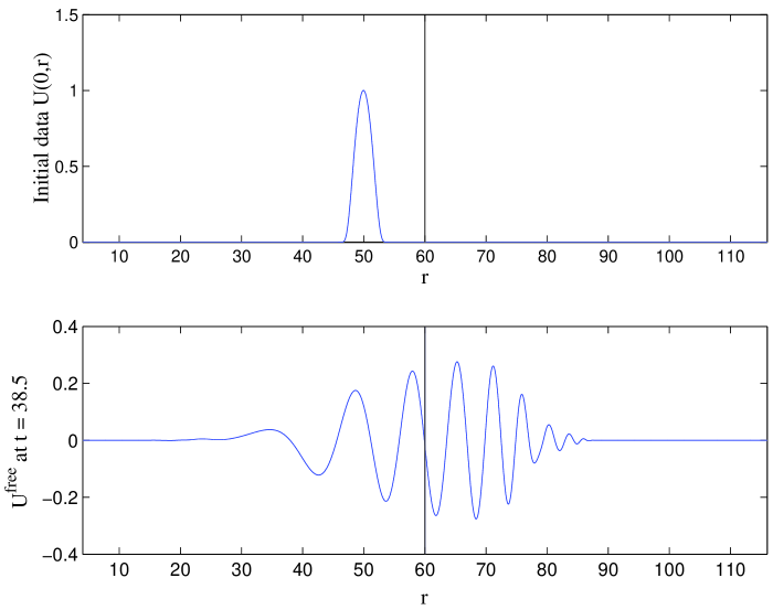
Figure 34. Free evolution on a larger domain. The parameters for the evolution are $\Delta t\big{/}\Delta r=0.5$, $\mathrm{m}=2$, $l=64$, and $\jmath=2$. There are $32768$ subintervals dividing $[4,116]$ and 16384 subintervals dividing $[4,60]$.

In order to generate an accurate reference solution, we numerically evolve the initial data on the larger domain $[4,116]$ until $t=38.5$. For this evolution (and all others in this subsection) we choose a Courant factor $\Delta t\big{/}\Delta r=0.5$, and at $r_{2Q}=116$ we use simple copy–over boundary conditions, since the disturbance does not reach this farther outer boundary in the short time $t=38.5$. The result of our numerical evolution on $[4,116]$ is a numerical solution $U^{\mathrm{free}}$, described as “free” since it arises from a free evolution. Any numerical error in $U^{\mathrm{free}}$ stems solely from the finite difference scheme and not from boundary conditions. The bottom plot in Fig. 34 depicts the result of such an evolution for the case $l=64$ and $\jmath=2$ (gravitational radiation). In both this plot and the plot of the initial data above it, we have indicated $r_{B}=60$ by a vertical line. The free solution that we compute corresponds to $2^{14}$ subintervals of $[4,60]$ and so $2^{15}$ subintervals of $[4,116]$. Over the smaller domain $[4,60]$, we have estimated that

(175) $$\|\Delta U^{\mathrm{free}}\|_{\infty}=\mathrm{sup}\big{\{}|U^{\mathrm{free}}_{q}-U^{\mathrm{true}}_{q}|:q=0,\dots,16384\big{\}}\simeq 3.6\times 10^{-6}\,,$$

where the $U^{\mathrm{true}}_{q}$ are exact mesh–point values of the true solution. Notice that this supremum error measure is computed with truncated arrays (the full range of $q$ is $0$ to $32768$). We have obtained this estimate by a suitable convergence analysis of the truncated free solution and Richardson extrapolation [62].

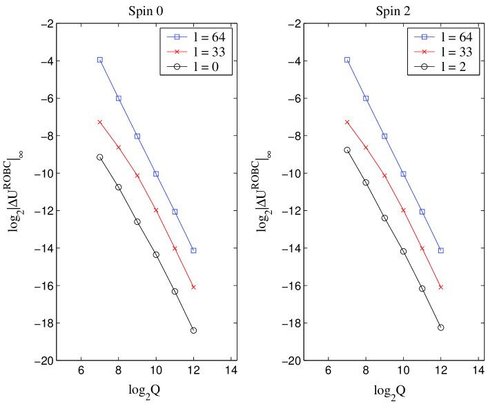
Figure 35. Error of the solution $U^{\mathrm{ROBC}}$. We plot the absolute supremum error of the robc solution for various $j$, $l$, and $Q$. In all cases, these errors have been computed with the free solution corresponding to $2^{14}$ subintervals of $[4,60]$ in place of the true solution.

Using our $\varepsilon=10^{-10}$ robc, we may also evolve the initial data to $t=38.5$ directly on the smaller domain $[4,60]$, thereby generating another numerical solution $U^{\mathrm{ROBC}}$. Furthermore, we may generate yet another numerical solution $U^{\mathrm{SOBC}}$ by using Sommerfeld outer boundary conditions (sobc) in place of our robc. By sobc we mean the local boundary conditions defined by setting the numerical kernel $\Xi_{l}=0$ throughout the evolution. The short–time numerical tests at hand then amount to numerical examinations of the convergence and accuracy of both $U^{\mathrm{ROBC}}$ and $U^{\mathrm{SOBC}}$ relative to the free solution $U^{\mathrm{free}}$ (here serving in lieu of the true solution). Let us first consider the issue of convergence in the next paragraph, and afterwards turn to accuracy.

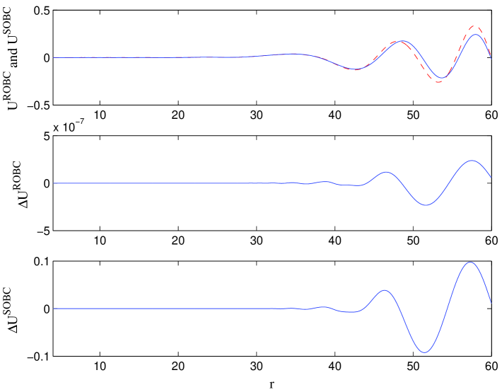
Figure 36. Comparison of robc and sobc. Here $\jmath=2$, $l=64$, and all profiles have been computed with 16384 subintervals of $[4,60]$. In the top plot the $U^{\mathrm{SOBC}}$ solution is the dashed line.

Suppose $U^{\mathrm{ROBC}}$ is obtained for $Q=2^{8}$, with the supremum error $\|\Delta U^{\mathrm{ROBC}}\|_{\infty}$ between $U^{\mathrm{ROBC}}$ and $U^{\mathrm{free}}$ is given by the formula

(176) $$\|\Delta U^{\mathrm{ROBC}}\|_{\infty}=\mathrm{sup}\big{\{}|U^{\mathrm{ROBC}}_{q}-U^{\mathrm{free}}_{64q}|:q=0,\dots,256\big{\}}\,,$$

where we note that $64=2^{14}/2^{8}$. In general, a stride of $2^{14}/2^{k}$ must be used to evaluate $\|\Delta U^{\mathrm{ROBC}}\|_{\infty}$, when the array $U^{\mathrm{ROBC}}$ corresponds to $Q=2^{k}$ for $k\leq 14$ (and $U^{\mathrm{free}}$ corresponds to $2^{14}$ subintervals of $[4,60]$ as set up above). Let us switch to matlab notation for such norms, so that (176) becomes

(177) $$\|\Delta U^{\mathrm{ROBC}}\|_{\infty}=\mathrm{norm}\big{(}U^{\mathrm{ROBC}}(0:256)-U^{\mathrm{free}}(0:64:16384),\mathrm{inf}\big{)}\,.$$

As we increase the number of subintervals used to compute $U^{\mathrm{ROBC}}$, we can check to see if the robc numerical solution initially converges to the free one. The plots in Fig. 35 document this convergence for a small sampling of $\jmath$ and $l$ values. Due to the equal scales of their horizontal and vertical axes, these plots indicate that our implementation of robc is second–order accurate as expected. Using L2 errors instead of supremum errors, we obtain the same convergence rates as those indicated. Plots analogous to those in Fig. 35 indicate that for any choice of $\jmath$ and $l$ values in our sampling the corresponding numerical solution $U^{\mathrm{SOBC}}$ does not converge to the free solution.

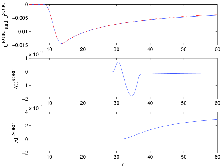
Figure 37. Comparison of robc and sobc. Here $\jmath=0$, $l=0$, and all profiles have been computed with 16384 subintervals of $[4,60]$. In the top plot the $U^{\mathrm{SOBC}}$ solution is the dashed line.

Let us now consider the accuracy of both the robc and sobc solutions, fixing for both a spatial resolution of $2^{14}$ subintervals of $[4,60]$, the same resolution as for $U^{\mathrm{free}}$. For the choices $\jmath=2$ and $l=64$, Fig. 36 depicts the numerical solutions $U^{\mathrm{ROBC}}$ and $U^{\mathrm{SOBC}}$ as well as the errors $\Delta U^{\mathrm{ROBC}}=U^{\mathrm{ROBC}}-U^{\mathrm{free}}$ and $\Delta U^{\mathrm{SOBC}}=U^{\mathrm{SOBC}}-U^{\mathrm{free}}$. Fig. 37 depicts the same plots, but for $\jmath=0$ and $l=0$. For the sake of comparison, the top plots in these figures superimpose $U^{\mathrm{ROBC}}$ and $U^{\mathrm{SOBC}}$. That they differ is even evident to the eye, and a glance at the middle and bottom plots in the figures shows that the sobc errors are many orders of magnitude larger than the robc errors. For the $\jmath=2$ and $l=64$ case shown in Fig. 36, we note that $\|\Delta U^{\mathrm{ROBC}}\|_{\infty}$ (now computed with a stride of one) is about $2.38\times 10^{-7}$. This value is smaller than $3.6\times 10^{-6}$, our aforementioned estimate for the supremum error

(178) $$\|\Delta U^{\mathrm{free}}\|_{\infty}=\mathrm{norm}\big{(}U^{\mathrm{free}}(0:16384)-U^{\mathrm{true}}(0:16384),\mathrm{inf}\big{)}$$

in the free solution. In Table 8 we list these error measures for the other values of $\jmath$ and $l$ in our small sampling. In all cases the robc and free numerical solutions agree to within our confidence in the free solution. On the contrary, the sobc and free numerical solutions do not agree to within this confidence, as is evident from the errors $\|\Delta U^{\mathrm{SOBC}}\|_{\infty}$ also listed in the table.

$l$	$\|\Delta U^{\mathrm{free}}\|_{\infty}$	$\|\Delta U^{\mathrm{ROBC}}\|_{\infty}$	$\|\Delta U^{\mathrm{ROBC}}\|_{\infty}$	$\|\Delta U^{\mathrm{SOBC}}\|_{\infty}$
$64$	$3.6\times 10^{-6}$	$2.46\times 10^{-7}$	$2.38\times 10^{-7}$	$9.80\times 10^{-2}$
$33$	$9.7\times 10^{-7}$	$5.97\times 10^{-8}$	$5.65\times 10^{-8}$	$7.21\times 10^{-2}$
$0$	$1.9\times 10^{-7}$	$1.77\times 10^{-9}$	$1.78\times 10^{-9}$	$2.88\times 10^{-4}$

Table 8. Error measures for short–time test. The table lists various supremum error measures for the $\jmath=0$ case (the corresponding errors for $\jmath=2$ look the same). The first column of values for $\|\Delta U^{\mathrm{free}}\|_{\infty}$ are estimates for the error in the free solution, and we have obtained these estimates via a convergence analysis of the free evolution. In the last column, for example, the values $\|\Delta U^{\mathrm{SOBC}}\|_{\infty}$ measure the difference between the free and sobc solutions when both are computed with a spatial resolution of 16384 subintervals. We list two columns for $\|\Delta U^{\mathrm{ROBC}}\|_{\infty}$. The first corresponds to $\varepsilon=10^{-6}$ and the second to $\varepsilon=10^{-10}$ robc. We see essentially no difference between these at the resolution of this test.

5.1.2. Long–time evolutions

We consider three long–time evolutions, taking for the first two $\jmath=2$, $l=2$, and $\Delta t\big{/}\Delta r=0.5$ for all runs. Moreover, for the first two we choose initial data $U(0,r)=f(r)/r$ with $f(r)$ as before in (174), but now with for $A=10$, $a=5$, $b=15$, and $\delta=20$. The profile $U(0,r)$ is then a compactly supported bump function of unit height on $[5,15]$, an interval overlapping the circular photon orbit at $3\mathrm{m}=6$ [52]. We again set $X(0,r)=-U(0,r)/r$ in order to crudely mimic outgoing initial data. Such data describes a wave packet that, although initially close to the horizon, somewhat escapes from the blackhole. For both evolutions, we consider a numerical test of our robc. Each one amounts to comparing a numerical solution $U^{\mathrm{ROBC}}$ generated with our robc to a numerical solution $U^{\mathrm{free}}$ generated on a larger domain, now either four or sixteen times the size of $[4,60]$.

These long–time tests show that our robc yield accurate numerical solutions corresponding to certain celebrated physical phenomena. In addition, the first long–time test further elucidates the error properties of the robc solution relative to the free one. Assuming that $U^{\mathrm{ROBC}}$ and $U^{\mathrm{free}}$ are obtained at the same spatial resolution, any difference $\|U^{\mathrm{ROBC}}-U^{\mathrm{free}}\|_{\infty}$ between them stems from three possible sources: (i) use of an approximate kernel in the integral convolution at the boundary, (ii) the integration rule used to evaluate the integral convolution, and (iii) error in the boundary values of the solution $U$ itself (which are fed into the convolution). Source (iii) has the potential for feedback. Our first long–time evolution and experiment examines the competing influence of these sources. Based on this examination, we will conclude (to no surprise) that, given our second–order–accurate scheme for interior update, our trapezoidal implementation of the robc is optimal.

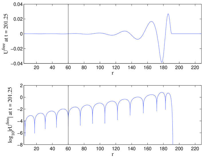
Figure 38. Free evolution on $[4,228]$ at $t=201.25$.

First long–time evolution: quasinormal ringing. For the first test, we evolve the data on $[4,228]$ until $t=201.25$, thereby obtaining a new free solution. The top plot in Fig. 38 depicts this free solution. Notice that the leading edge of the front has advanced from $r=15$ to about $r=200$, and that overall the disturbance falls off rapidly with decreasing $r$. However, the bottom plot, a graph of the base–10 logarithm of the absolute value of $rU^{\mathrm{free}}$ (with multiplication by $r$ correcting for $1/r$ fall–off in amplitude), exhibits the behavior called quasinormal ringing in the physics literature. This behavior is also depicted in Fig. 39 which shows the free evolution of the same data on $[4,900]$ until $t=700$. As the leading front advances, it leaves exponentially decaying oscillations in its wake. The phenomenon is better described by examining the time history of the solution at a fixed radius, as is done in Fig. 40. The complex frequency corresponding to this behavior is the least–damped (or fundamental) $l=2$ quasinormal mode of the $\mathrm{m}=2$ blackhole in question. Kokkotas and Schmidt record a value of $0.37367-{\rm i}0.08896$ for the product of this frequency and the blackhole mass [68]. Dividing this value by 2, we find $0.186835-\mathrm{i}0.04448$ as the least–damped $l=2$ quasinormal mode of our black hole. The estimate $\pi/0.186835\simeq 16.8$ indeed corresponds to about half a wavelength in the lefthand plot of Fig. 40 (as measured from one spike to the next), and the damping coefficient $0.04448/\ln 10\simeq 0.019$ matches minus the slope of the decaying amplitude in the same plot.

To further examine the error properties of the robc solution, we generate the numerical solution $U^{\mathrm{ROBC}}$ on $[4,60]$ for $t=201.25$, that we may compare it with $U^{\mathrm{free}}$ restricted to this smaller interval. The outer radius $r_{B}=60$ is marked by a black line in Fig. 38. Using matlab notation, for $Q$ subdivisions of $[4,60]$ we have the numerical solution $U^{\mathrm{ROBC}}(0:Q)$, and for $4Q$ subdivisions of $[4,228]$ we have the numerical solution $U^{\mathrm{free}}(0:4Q)$. We may then compare the truncated solution $U^{\mathrm{free}}(0:Q)$ directly with $U^{\mathrm{ROBC}}(0:Q)$ by computing the supremum error between the two. Doing so for a sequence of spatial resolutions, we construct the column labeled trapezoidal in Table 9. By changing the spatial resolution with $\Delta t\big{/}\Delta r=0.5$ fixed, we also change the number of temporal steps taken in generating each solution; however, we always compare robc and free solutions generated with the same number of temporal steps. Taking the base–2 logarithm of successive ratios of the trapezoidal errors in Table 9, we see a second–order convergence. Such convergence indicates that source (i) from the paragraph before last is not the dominant contribution to $\|U^{\mathrm{ROBC}}-U^{\mathrm{free}}\|_{\infty}$. Indeed, we have the same approximating numerical kernel regardless of mesh resolution. Therefore, for the numerical experiment at hand (which is based on our trapezoidal implementation of the robc) this error measure stems chiefly from the aforementioned sources (ii) and (iii).

Q	rectangular	trapezoidal	parabolic
256	$1.6571\times 10^{-5}$	$7.2426\times 10^{-7}$	$6.8587\times 10^{-7}$
512	$8.3088\times 10^{-6}$	$1.7819\times 10^{-7}$	$1.6877\times 10^{-7}$
1024	$4.1663\times 10^{-6}$	$4.3814\times 10^{-8}$	$4.1495\times 10^{-8}$
2048	$2.0843\times 10^{-6}$	$1.0856\times 10^{-8}$	$1.0278\times 10^{-8}$
4096	$1.0416\times 10^{-6}$	$2.7074\times 10^{-9}$	$2.5627\times 10^{-9}$
8192	$5.2053\times 10^{-7}$	$6.7626\times 10^{-10}$	$6.4011\times 10^{-10}$
16384	$2.6023\times 10^{-7}$	$1.6888\times 10^{-10}$	$1.5985\times 10^{-10}$
32768	$1.3011\times 10^{-7}$	$4.2149\times 10^{-11}$	$3.9891\times 10^{-11}$

Table 9. Supremum errors for first long–time test. We list errors $\mathrm{norm}\big{(}U^{\mathrm{ROBC}}(0:Q)-U^{\mathrm{free}}(0:Q),\mathrm{inf}\big{)}$ corresponding to (forward) rectangular, trapezoidal, and parabolic implementations of the robc.

To further resolve the influence of these error sources, we have carried out the experiment using the rectangle rule (both forward and backward cases), rather than the trapezoid rule as in (167), to evaluate the local part of the boundary Laplace convolution. The corresponding errors for either case, with those for the forward case listed in the first column of Table 9, decrease at a first–order rate. Therefore, we conclude that for a rectangular implementation the dominant contribution to $\|U^{\mathrm{ROBC}}-U^{\mathrm{free}}\|_{\infty}$ is source (ii). We have also carried out the experiment using Simpson’s rule (parabolic rule) to approximate the local part of the convolution. Doing so involves a certain parabolic interpolation to get half–time–step numerical values for the field $U$. In this case, the corresponding errors, listed in the third column of Table 9, again decrease at a second–order rate, although these errors are slightly smaller than their trapezoid counterparts. If (ii) were the dominant contribution to $\|U^{\mathrm{ROBC}}-U^{\mathrm{free}}\|_{\infty}$ for our trapezoidal implementation of the robc, then switching to a parabolic implementation should lead to error decrease at a fourth–order rate. Since it does not, we conclude that our trapezoidal robc are not the dominant source of error (assuming a second–order interior scheme). These considerations suggest that there is little point in improving the integration rule used for the Laplace convolution, unless one also implements a higher order scheme for the interior.

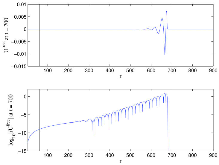
Figure 39. Free evolution on $[4,900]$ at $t=700$.

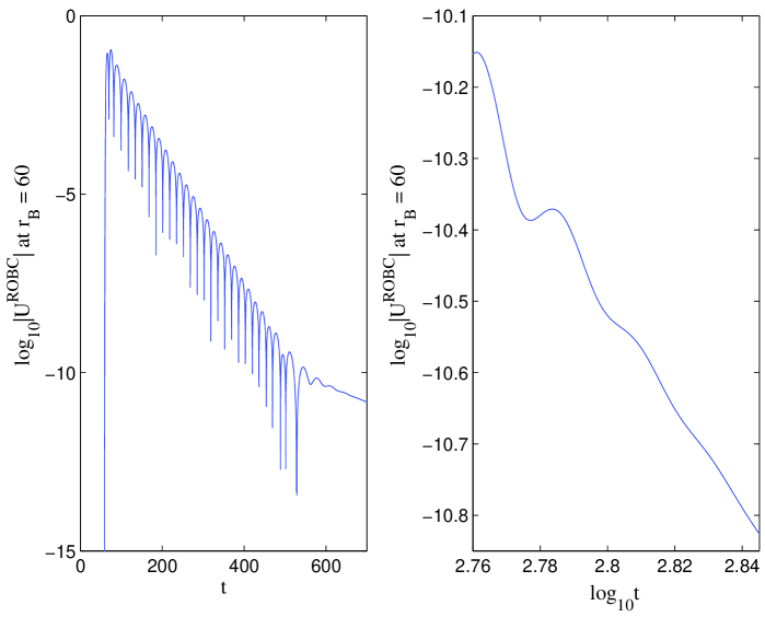
Figure 40. Quasinormal ringing and decay tail. For the described second long–time evolution, we record the time history of the field at the fixed position $r_{B}=60$ (the vertical line in Fig. 39). The lefthand plot depicts quasinormal ringing. The righthand plot, a zoom–in of the late–time history of the field, features $\log_{10}t$ to highlight the onset of the $t^{-7}$ power–law decay. Each plot is a history of the numerical boundary value $U^{\mathrm{ROBC}}_{Q}$.

Second long–time evolution: decay tails. Our second long–time, one–dimensional, test evolution shows that the robc yield a reasonably accurate numerical solution even for very late times relative to the crossing time of the domain. After the quasinormal ringing dies down, the solution at a fixed radius $r$ is known to behave as order $t^{-(2l+3)}$, provided the initial field configuration is not time–symmetric [68], and this behavior is seen in the righthand plot of Fig. 40. Heuristically, this late–time decay tail stems from the back–scattering of outgoing waves off of the background curvature. Fig. 39 depicts the solution at $t=700$, and the bottom plot shows that by this late time a sizable region has entered the power–law decay regime. Note that $r_{B}=60$ is again marked by a black line in the figure. For $Q$ subdivisions of $[4,60]$, there are $16Q$ subdivisions of $[4,900]$. Therefore, we truncate the full numerical solution $U^{\mathrm{free}}(0:16Q)$, and like before compare $U^{\mathrm{free}}(0:Q)$ directly with $U^{\mathrm{ROBC}}(0:Q)$. Doing so for a sequence of spatial resolutions, we construct Table 10. Due to round–off error, these errors do not decrease at a second–order rate. However, with the spatial resolution $4096$ indicated in the table’s fifth row as an example, we note that the supremum relative error

(179) $$\mathrm{norm}((U^{\mathrm{free}}(0:4096)-U^{\mathrm{ROBC}}(0:4096))./U^{\mathrm{free}}(0:4096),\mathrm{inf})$$

is the reasonably accurate value $2.1019\times 10^{-4}$. For sobc, rather than $6.0051\times 10^{-16}$ for the absolute error and $2.1019\times 10^{-4}$ for the relative error, we get the numbers $2.9569\times 10^{-9}$ and $5.2668\times 10^{3}$. Fig. 41 depicts the solution at $t=700$ on $[4,60]$. The top plot superimposes both $U^{\mathrm{free}}(0:4096)$ and $U^{\mathrm{ROBC}}(0:4096)$ to show that they match to the eye.

In the bottom plot of Fig. 41 we show a modified $U^{\mathrm{ROBC}}(0:4096)$. This profile has been generated by “turning off” the cut contribution to the kernel. More precisely, to obtain this profile, in (159) we have by hand set $H_{i}(t-t^{\prime})=0$, $\forall i$ throughout the evolution. For this $l=2$ case, the kernel $\Xi(t)=G_{1}(t)$ in (156) then corresponds to a single conjugate pair of poles. From this experiment, we might infer that the phenomenon of decay tails is handled by the cut contribution to the kernel. As seen in Sections 3.1 and 3.2 (but there for $\jmath=0$), this contribution stems from a continuous distribution of poles.

$\mathrm{norm}\big{(}U^{\mathrm{ROBC}}(0:256)-U^{\mathrm{free}}(0:256),\mathrm{inf}\big{)}$	$1.8166\times 10^{-15}$
$\mathrm{norm}\big{(}U^{\mathrm{ROBC}}(0:512)-U^{\mathrm{free}}(0:512),\mathrm{inf}\big{)}$	$1.1427\times 10^{-15}$
$\mathrm{norm}\big{(}U^{\mathrm{ROBC}}(0:1024)-U^{\mathrm{free}}(0:1024),\mathrm{inf}\big{)}$	$7.6272\times 10^{-16}$
$\mathrm{norm}\big{(}U^{\mathrm{ROBC}}(0:2048)-U^{\mathrm{free}}(0:2048),\mathrm{inf}\big{)}$	$6.2889\times 10^{-16}$
$\mathrm{norm}\big{(}U^{\mathrm{ROBC}}(0:4096)-U^{\mathrm{free}}(0:4096),\mathrm{inf}\big{)}$	$6.0051\times 10^{-16}$
$\mathrm{norm}\big{(}U^{\mathrm{ROBC}}(0:8192)-U^{\mathrm{free}}(0:8192),\mathrm{inf}\big{)}$	$5.9483\times 10^{-16}$

Table 10. Supremum errors for second long–time test. Here we are using matlab notation for the supremum error as explained in the text.

Third long–time evolution: decay tails revisited. Here we consider an experiment described by Allen, Buckmiller, Burko, and Price [36], in order to further demonstrate that our robc capture the phenomenon of decay tails. In terms of the standard retarded time $u=T-r_{*}$, we introduce a function $f(u)=\big{[}u(u-8\mathrm{m})/(16\mathrm{m}^{2})\big{]}{}^{8}$ for $0\leq u\leq 8\mathrm{m}$, with $f(u)=0$ otherwise. Since we work with Eddington–Finkelstein coordinates, whereas [36] worked with static time coordinates, we set $u(t,r)=t+r-2r_{*}-C$. Here $C$ is a constant, chosen to ensure that $C+2\mathrm{m}\log[-1+C/(2\mathrm{m})]=0$, and in turn $u(t,C)=t$. [Before in (121) and the analysis following that equation, $t$ denoted a time variable which differs from this one by a constant, but no matter.] We obtain an initial $\jmath,l=0$ scalar wave packet as $U(0,r)=f(u(0,r))/r$, and also complete the data accordingly with $X(0,r)$ obtained from (129). That is, we get $X(0,r)$ by computing $e_{+}[f(u(t,r))/r]$ and then setting $t=0$. Therefore, the data describes an essentially outgoing pulse which at $t=0$ is of unit height and roughly supported on $[2\mathrm{m},C]$. Next, on a numerical domain $[2\mathrm{m},30\mathrm{m}]$, we evolve the data until $t=1000\mathrm{m}$ with our $\varepsilon=10^{-10}$ robc, along the way recording the time history of the product $rU^{\mathrm{ROBC}}$ of radius and numerical field at the fixed radius $C$ (more precisely, at the radial mesh point closest to $C$). Here we multiply by radius (whereas in Fig. 40 we did not) in order to have better agreement with [36]. The resulting history is shown in Fig. 42. We stress that our domain size is more than 16 times smaller than the one considered in [36].

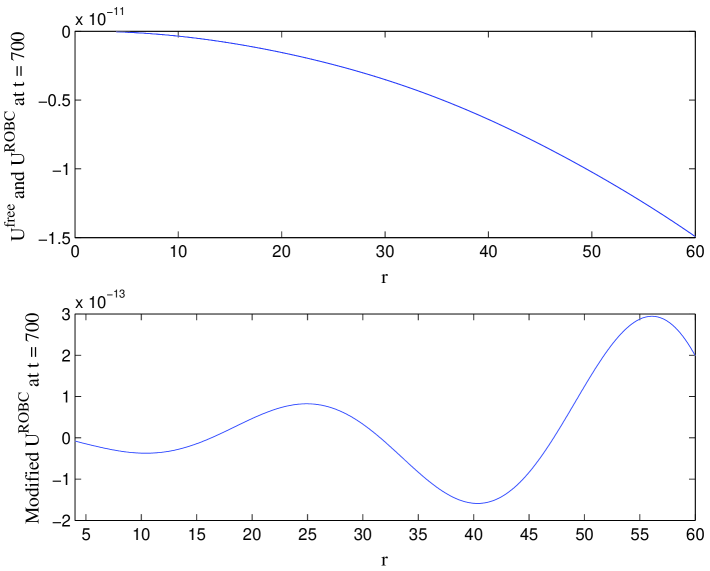
Figure 41. $U^{\mathrm{free}}$ and $U^{\mathrm{ROBC}}$ at $t=700$. The modified $U^{\mathrm{ROBC}}$ solution has been obtained by removing the cut contribution to the tdrk as described in the text.

We believe this experiment shows that our robc indeed resolve decay tails. This is not to say that the results of [36] are incorrect. Those results are applicable for the type of boundary conditions considered, namely approximate conditions which are not history dependent. We intend to carry out other more careful tests of our robc along the lines spelled out in [36]. Results will be presented in a forthcoming work [67].

5.2. Three–dimensional evolution

Our final test is three–dimensional, and considers the scenario of a wave–packet striking the computational boundary at a shallow angle (or at least not on a perpendicular). Such a scenario is known to be difficult test case for radiation boundary conditions in flatspace. We carry out this test only for the scalar $\jmath=0$ case.

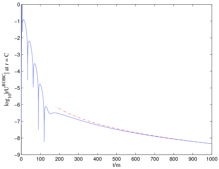
Figure 42. Long–time history of the field $rU^{\mathrm{ROBC}}$ at $r=C\simeq 2.5569\mathrm{m}$. Here we show the result of the third long–time experiment with $\jmath,l=0$ and initial data inspired by [36]. $C$ is the radial value corresponding to vanishing tortoise coordinate. More precisely, here we consider the history at the radial mesh point $\simeq 2.5572\mathrm{m}$ closest to $C$. This plot may be compared with Figure 2 in [36]. The dash–dot line is the base–10 logarithm of $4.57(\mathrm{m}/t)^{3}$, similar to the matching curve considered in [36]. This plot exhibits the power–law decay of the field. We stress that this plot has been obtained with the outer boundary radius $r_{B}=30\mathrm{m}$. In carrying out the experiment, we set $\mathrm{m}=2$.

5.2.1. Description and set–up

Consider the bump function

(180) $$f(t,x,y,z)=A\exp\left(\frac{2\delta}{b^{2}}\right)\left/\exp\left[\frac{\delta}{\big{(}\big{|}\mathbf{r}-\mathbf{v}t-\mathbf{r}_{0}\big{|}+b\big{)}{}^{2}}+\frac{\delta}{\big{(}b-\big{|}\mathbf{r}-\mathbf{v}t-\mathbf{r}_{0}\big{|}\big{)}{}^{2}}\right]\right.\,,$$

where

(181) $$\big{|}\mathbf{r}-\mathbf{v}t-\mathbf{r}_{0}\big{|}=\big{[}(x-v_{x}t-x_{0})^{2}+(y-v_{y}t-y_{0})^{2}+(z-v_{z}t-z_{0})^{2}\big{]}^{1/2}\,.$$

Were we considering wave propagation on flat Minkowski spacetime, $f$ would be an exact solution. Were this the case, the bump function would have center $\mathbf{r}_{0}=(x_{0},y_{0},z_{0})$ at $t=0$ and would travel without distortion and at unit speed in the direction $\mathbf{v}=(v_{x},v_{y},v_{z})$. Here we are assuming that $v_{x}^{2}+v_{y}^{2}+v_{z}^{2}=1$.

Let us interpret $(x,y,z)$ as the “Cartesian coordinates” belonging to the Eddington–Finkelstein coordinates $(r,\theta,\phi)$ from Section 4.1.1 (the same spatial coordinates as in Section 1.1.1). That is to say, $x=r\sin\theta\cos\phi$, and so on. Doing so gives us a diffeomorphism between the initial Schwarzschild time slice $\Sigma$ and three–dimensional Euclidean space $\mathbb{E}^{3}$, itself viewed as the initial surface of flat spacetime. On $\mathbb{E}^{3}$ we obtain the data $f|_{t=0}$ and $\partial_{t}f|_{t=0}$ which is then taken over as initial data on $\Sigma$. The Schwarzschild evolution of this data is not the spacetime function (180). Nevertheless, on physical grounds, one expects this evolution to be qualitatively similar to the flat–spacetime evolution (180) of the same data, provided that (i) the center $(x_{0},y_{0},z_{0})$ is of large enough radius $(x_{0}^{2}+y_{0}^{2}+z_{0}^{2})^{1/2}$ and (ii) the support $b$ relative to that center is small enough.

We have written a three–dimensional spectral code to evolve such data. The basic idea, implemented numerically, is to obtain a data set, $U_{lm}(0,r)$ and $X_{lm}(0,r)$, for each spherical mode $(l,m)$, a set we then evolve via the one–dimensional purely radial scheme described in Section 4 (although throughout that section we suppressed the $lm$ subscripts on these mode variables). The exact data for each mode are obtained by harmonic analysis as follows:

(182) $$U_{lm}(0,r)=\int_{0}^{2\pi}\int_{0}^{\pi}f(0,x(r,\theta,\phi),y(r,\theta,\phi),z(r,\theta,\phi))\overline{Y}_{lm}(\theta,\phi)\sin^{2}\theta{\rm d}\theta{\rm d}\phi,$$

and

(183) $$X_{lm}(0,r)=\int_{0}^{2\pi}\int_{0}^{\pi}g(0,x(r,\theta,\phi),y(r,\theta,\phi),z(r,\theta,\phi))\overline{Y}_{lm}(\theta,\phi)\sin^{2}\theta{\rm d}\theta{\rm d}\phi,$$

where $g=\partial_{t}f+r^{-1}(x\partial_{x}f+y\partial_{y}f+z\partial_{z}f)$. After all one–dimensional evolutions have been carried out, we have a collection of $U_{lm}(t,r)$ modes (here viewed as exact for ease of presentation) with which we can construct the three–dimensional solution

(184) $$U(t,r,\theta,\phi)=\sum_{l=0}^{\infty}\sum_{m=-l}^{l}U_{lm}(t,r)Y_{lm}(\theta,\phi)$$

via harmonic synthesis. Numerically, we obtain $f|_{t=0}$ and $g|_{t=0}$ on a spherical–polar grid

(185) $$\big{\{}(r_{q},\theta_{i},\phi_{j}):0\leq q\leq Q,1\leq i\leq I,1\leq j\leq J\big{\}}$$

by exact function calls. For each $r_{q}$ we then perform a harmonic analysis on the restriction of the initial data to the two–dimensional spherical grid $(\theta_{i},\phi_{j})$. We have used Adams and Swarztrauber’s spherepack 3.0 to numerically perform all harmonic analysis and synthesis, and in particular those subroutines (shagci, shagc, shsgci, and shsgc) from spherepack which take the $\theta_{i}$ as Gaussian points in colatitude.

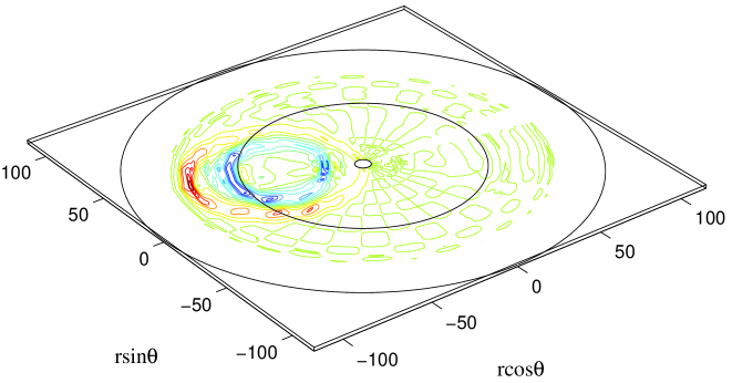
Figure 43. Equatorial cross section of $U^{\mathrm{free}}$ at $t=38.5$. The initial data for this evolution is described in the text. The outer, middle, and inner circles are $r=116$, $60$, and $4$. For this plot $(Q,I,J)=(2048,33,32)$, so that the shown spherical domain (determined by $4\leq r\leq 116$) corresponds to a $(4096,33,32)$ discretization. The oscillations spread out over the whole angular domain result from the harmonic truncation of the initial data.

We work with an angular grid corresponding to $(I,J)=(33,32)$, with the first number odd so that the equator is a Gaussian point. The spectral truncation in spherepack is triangular, and with this angular resolution we only sample harmonic modes for $l\leq 32$. Prior to the harmonic analysis described above, we perform a preliminary analysis followed immediately by synthesis. This initial procedure corresponds to truncation of the full harmonic series for $f|_{t=0}$ and $g|_{t=0}$, and it does modify of the described initial data. The resulting data is now spread out over the whole angular domain, although it remains concentrated at $(x_{0},y_{0},z_{0})$.

5.2.2. Short–time three–dimensional evolution

The three–dimensional numerical test we now describe is somewhat analogous to the one–dimensional short–time test described in Section 5.1.1. We consider a spherical domain bounded internally by $r=4$ and externally by $r=116$. On this large domain, we choose initial data as described in the last subsubsection. That is to say, in addition to the discretization sizes $(Q,I=33,J=32)$ of our three–dimensional domain, in (180) we also choose the vectors $(x_{0},y_{0},z_{0})$ and $(v_{x},v_{y},v_{z})$ as well as the values of $A$, $\delta$, and $b$. We then numerically evolve this data until $t=38.5$. In setting up the initial data, due care must be taken to ensure that (i) the support of the data is contained within $r<60$ and (ii) in the short–time $t=38.5$ the propagating solution spills over $r=60$ but does not reach $r=116$. To satisfy these criteria, we have chosen a bump function (180) centered at $(x_{0},y_{0},z_{0})=(-40,20,14)$, with initial velocity $(v_{x},v_{y},v_{z})=(-0.87,-0.4,-0.3)$. Moreover, we have chosen $A=1$, $b=12$, and $\delta=0.1$.

The byproduct of our evolution is a three–dimensional free solution $U^{\mathrm{free}}$ at $t=38.5$. As before, any numerical error in $U^{\mathrm{free}}$ stems solely from the finite–difference scheme and not the boundary conditions. Having generated such a free solution from the initial data described above, we show the result in Fig. 43, a depiction of the equatorial cross section of $U^{\mathrm{free}}$. As mentioned, the number $I=33$ of $\theta_{i}$ points ensures that $\theta_{17}=\pi/2$, allowing for such a figure. Our initial data has been designed to yield an evolution with an interesting cross section.

$Q$	$\|\Delta U^{\mathrm{ROBC}}\|_{\infty}$	$\|\Delta U^{\mathrm{ROBC}}\|_{2}$	$\|\Delta U^{\mathrm{SOBC}}\|_{\infty}$	$\|\Delta U^{\mathrm{SOBC}}\|_{2}$
$256$	$1.7593\times 10^{-4}$	$4.9594\times 10^{-6}$	$7.3416\times 10^{-2}$	$8.3218\times 10^{-3}$
$512$	$1.6646\times 10^{-5}$	$1.1387\times 10^{-6}$	$7.3137\times 10^{-2}$	$8.2895\times 10^{-3}$
$1024$	$3.4185\times 10^{-6}$	$2.7872\times 10^{-7}$	$7.3131\times 10^{-2}$	$8.2724\times 10^{-3}$
$2048$	$7.9344\times 10^{-7}$	$6.8970\times 10^{-8}$	$7.3131\times 10^{-2}$	$8.2656\times 10^{-3}$

Table 11. Error measures for the three–dimensional test.

The numerical test consists of again evolving the data, but now on the smaller spherical domain determined by $4\leq r\leq 60$ and using the $\varepsilon=10^{-10}$ robc. As a result, we get another three–dimensional array $U^{\mathrm{ROBC}}$ which we compare with a suitably truncated $U^{\mathrm{free}}$. Note that now both $U^{\mathrm{ROBC}}$ and $U^{\mathrm{free}}$ are three–dimensional arrays of physical values, whereas in the first subsection they stood for one–dimensional arrays of spectral values. We consider two error measures corresponding to the difference $\Delta U^{\mathrm{ROBC}}=U^{\mathrm{ROBC}}-U^{\mathrm{free}}$. The first is simply the absolute supremum error

(186) $$\|\Delta U^{\mathrm{ROBC}}\|_{\infty}=\mathrm{sup}\big{\{}\big{|}U^{\mathrm{ROBC}}_{q,i,j}-U^{\mathrm{free}}_{q,i,j}\big{|}:0\leq q\leq Q,1\leq i\leq I,1\leq j\leq J\big{\}}\,,$$

while the second is a discretization of the L2 error

(187) $$\|\Delta U^{\mathrm{ROBC}}\|_{2}=\frac{1}{\mathrm{vol}(\Sigma)}\left[\sum_{j=1}^{J}\sum_{i=1}^{I}\sum_{q=1}^{Q}\big{|}U^{\mathrm{ROBC}}_{q,i,j}-U^{\mathrm{free}}_{q,i,j}\big{|}{}^{2}M_{q}r^{2}_{q}\sin\theta_{i}\Delta r\Delta\theta_{i}\Delta\phi\right]^{1/2}\,,$$

where the radial lapse factor $M_{q}=(1+4/r_{q})^{1/2}$ ensures that this discretization corresponds to proper integration. The volume of the computational domain is

(188) $$\mathrm{vol}(\Sigma)=4\pi\int_{4}^{60}(1+4/r)^{1/2}r^{2}{\rm d}r\simeq 9.48255\times 10^{5}.$$

Since the $\theta$–mesh is comprised of Gaussian points $\theta_{i}$, we must also include the appropriate Gaussian weights $\Delta\theta_{i}$ in the sum (both the $\theta_{i}$ and $\Delta\theta_{i}$ are obtained with the routine gaqd from spherepack). We emphasize that unlike the situation in the first subsection where all error measures have been computed in the spectral space of spherical harmonics, these error measures are computed in physical space.

In Table 11 we list errors for the scenario shown in Fig. 43, doing so for radial discretizations corresponding to $Q=256$, $512$, $1024$ and $2048$ (so that the free solution has been computed with radial discretizations corresponding to $2Q=512$, $1024$, $2048$ and $4096$). In the table we have also listed the corresponding Sommerfeld errors, which have been computed as in (186) and (187) but with $U^{\mathrm{SOBC}}$ in place of $U^{\mathrm{ROBC}}$. Notice that the robc give rise to perfect second–order convergence, whereas the sobc do not. Moreover, the robc numerical solutions are several orders of magnitude more accurate than their sobc counterparts. It is also of interest to consider the relative computational cost of both robc and sobc. As sobc are purely local boundary conditions, they are of course less expensive than our robc. However, despite being strikingly more accurate, we find our robc to be nearly as cheap as sobc, as is evident by the relative timings listed in Table 12.

$Q$	robc	sobc
256	50.00	46.46
512	49.45	48.15
1024	43.21	41.85
2048	19.55	18.18

Table 12. Relative times for three–dimensional evolutions. Here we list the relative run times as percentages for the various $Q$ values. With $Q=1024$, for example, we generated the free solution on the larger domain via a run of 1817.26s. The corresponding robc and sobc runs on the smaller domain took 785.18s and 760.61s respectively. The entry 43.21 in the table corresponds to $100\times 785.18/1817.26$, and so on.

6. Discussion

We start this final section by comparing our results with those of our main reference [18], thereby gaining some perspective on what we have achieved. After that comparison we discuss possible applications and extensions.

6.1. Comparison with the work of Alpert, Greengard, and Hagstrom

Our rapid implementation of robc on the Schwarzschild geometry has been inspired by Alpert, Greengard, and Hagstrom’s implementation on flatspace. Although we have followed their approach closely, our implementation falls somewhat short of theirs. Let us point out why this is the case by comparing both implementations from theoretical and numerical standpoints.

From a theoretical perspective our work is less satisfactory than that of agh, chiefly because —as mentioned in the introduction— we are unable to give a rigorous asymptotic analysis of our implementation. For each angular $l$ index agh deal with a Bessel fdrk which is theoretically known to admit a sum–of–poles representation, one corresponding to a purely discrete sum in the case of 3+1 wave propagation and to a discrete and continuous sum in the 2+1 case. Moreover, due to the exhaustively studied properties of Bessel functions, they also start with a wealth of useful information about how the pole locations, pole strengths, and (in the 2+1 case) cut profile for the representation behave in all conceivable asymptotic regimes (which include certain scaling properties as $l$ becomes large). With tight control over where the physical poles accumulate and the behavior of cut profile, they are able to borrow ideas from the fast–multipole method in order to replace (discrete and continuous) physical pole sums with (fully discrete) approximate pole sums of fewer terms. As a result, they rigorously prove that the sum–of–poles representation for the Bessel fdrk admits a rational approximation, one uniformly valid in the righthalf frequency plane and exhibiting exponential convergence as the number of approximating poles is increased. For the scenario we have considered, such an analysis would seem out of the question. Indeed, although we have provided extremely convincing numerical evidence that the Heun fdrk admits a sum–of–poles representation, one strikingly similar to the 2+1 Bessel case, even this is conjecture from a theoretical standpoint. The battery of asymptotics needed to theoretically prove that such a representation admits a rational approximation in the style of agh is certainly well beyond the author’s knowledge of special functions.

Our numerical implementation of robc also falls somewhat short of agh’s, in that they considered a higher bandwidth (their $l\leq 1024$ compared to our $l\leq 64$) and a smaller best error tolerance (their $\varepsilon=10^{-15}$ compared to our $\varepsilon=10^{-10}$). However, we believe that on this count our work is closer to being on the same footing with theirs. Indeed, insofar as numerical implementation of flatspace robc is concerned, their elegant asymptotic analysis proving the existence of rational approximations is somewhat beside the point. Ultimately, their compression algorithm (which yields the desired rational approximations) relies only on the ability to evaluate the Bessel fdrk along the imaginary axis of the frequency plane. For Bessel functions, which obey certain order recursion relations, such evaluation can be efficiently done via the continued fraction expression (79) following from such relations. We stress that such evaluation requires no knowledge of the sum–of–poles representation for the kernel. Although we have no such continued fraction expression with which to evaluate the Heun fdrk, we have seen that our integration method is almost as accurate (in the sense spelled out by Section 2.2.4). For Bessel kernels we have observed that the numerical path integration required by our method is more expensive than continued fraction evaluation, and all the more so as the order $l+1/2$ gets large, although we have not made a systematic comparison of the two methods. However, the cost of evaluation is almost beside the point, since in principle any extra cost associated with our method need only be incurred once. Of true importance is accuracy, and through the use of extended precision we believe it possible to build Heun kernels corresponding to $\varepsilon=10^{-15}$ and through a bandwidth of $1024$. We point out that, insofar as both gravitational wave astronomy [69] and the post–Newtonian approximation [64, 70] of the gravitational field are concerned, $l$ values well below $64$ are the ones primarily relevant to gravitational wave observation.

Another numerical shortcoming of this work is that we have mainly considered certain discrete values of the outer boundary radius $\rho_{B}$, whereas agh allow for any value. We hope to extend our results to a continuous interval in $\rho_{B}$, say $[15,25]$, via construction of our rational approximations at Chebyshev nodes in $1/\rho_{B}$ and subsequent interpolation. The only reason we have not done this so far is that the straight compression algorithm described in Section 3.3 yields rational approximations which do not appear to vary that smoothly with $1/\rho_{B}$ (it is a nonlinear minimization after all). We anticipate that this problem can be mitigated. Indeed, using the described compression, one could construct a rational approximation at a Chebyshev node $\xi^{1}_{B}=1/\rho_{B}^{1}$ near 1/15, and as a result obtain a number of pole locations [the $Q$ in (101)]. For the other nodes, one could simply fix a $Q$ by suitable scaling of the collected locations for $\xi^{1}_{B}$, and then solve a straight least squares problem for $P$ in (101). This straight least–square solve would be the same problem as (101) but with $Q$ fixed. In any case, we do plan to build up some form of our robc which is valid over a continuous $\rho_{B}$ interval.

6.2. Potential applications and extensions

We briefly describe several potential applications of our robc. The first arises in the theory of non–spherical stellar collapse [52]. A massive star, having expended its nuclear fuel, will collapse into a blackhole, with gravitational waves radiated in the process. Provided that the initial configuration of the collapsing system is not highly non–spherical, the evolution of such waves are governed by the Regge–Wheeler and Zerilli equations. Our robc are therefore applicable to such scenarios. The classic work on perturbed Oppenheimer–Snyder collapse is that of Cunningham, Moncrief, and Price [71, 72], but we hope to carry out further numerical investigations with our robc. Another field of recent interest where our robc should find application is the theory of stellar perturbations, in particular oscillation modes of stars as sources for gravitational radiation (see for example [73, 74, 75]). As a third application, we anticipate that our robc can by applied to the Cauchy–perturbative matching scheme of Rupright, Abrahams, and Rezzolla [31, 32], a numerical approach to robc for full general relativity. The idea is to match the Cauchy evolution of the full Einstein equations to a set of one–dimensional, linear, radial evolutions of perturbative modes on Schwarzschild, with the matching taking place at an extraction two–surface large enough to ensure the validity of perturbation theory. In this approach, each of the modes is separately evolved on a large radial domain until the next time–step, allowing for both wave–form extraction and updating of the interior solution at the extraction surface. The equation governing the evolution of such modes is related to the one we have considered. Rupright et al employ Sommerfeld outer boundary conditions for their radial evolutions. We expect that our robc could improve their method, perhaps even doing away with the separate radial evolutions altogether (the idea here would be to impose our robc directly at the extraction surface, provided it indeed sits well within the perturbative region).

Let us mention several other arenas where the issue of robc might be examined along the lines laid down here. The most obvious would be robc for time–domain wave propagation on more complicated blackholes: the Reissner–Nordstrøm solution (charged Schwarzschild), the rotating Kerr solution, and the charged Kerr solution (also known as Kerr–Newman) [52]. While tackling the problem of robc for a metric as complicated as the Kerr solution would be very difficult, one might first obtain robc for an approximate solution (to the Einstein equations) which exhibits rotation, such as the Brill–Cohen metric (see p. 699 of [52] and references therein). On a different track, robc might be investigated for other types of pde on the Schwarzschild geometry, such as curved–space versions of the Klein–Gordon or Euler equations. Implementation of robc for fluid equations on blackholes would have application in realistic studies of blackhole accretion. The methods of this work could be extended to the Schrödinger equation with a potential, like the Coulomb potential, which is not of compact support. (In his dissertation [63] Jiang studied robc for the Schrödinger equation via the agh approach, but only considered compactly supported potentials.) Implementation of robc in such a setting would involve the special function theory of Coulomb wave functions or the related Whittaker functions (both incarnations of confluent hypergeometric functions)[58, 59, 60]. Finally, we remark on a more practical possibility, namely, extension of these methods to the ordinary wave equation but expressed in prolate or oblate spheroidal coordinates [40]. Ref. [76] addresses computational issues associated with evaluating spheroidal wave functions. The issue of robc in this setting would be not unlike the issue for Kerr blackholes. In any case, the spheroidal wave equation is essentially the confluent Heun equation, so one might expect our methods to be applicable. Radiative boundary conditions which are tied to spheroidal surfaces might prove useful in modeling phenomena with slender geometries, such as those arising in antenna design (see Ref. [77] and references therein).

Yet another extension of our work would involve coupling robc to high–order interior schemes, such as the one described in [78] and [79], but without reduction of accuracy. This is a delicate issue pertinent to the simulation of waves on flatspace as well as on blackholes. We have presented a second–order accurate implementation of robc, but it would be beneficial to achieve a fourth or higher–order implementation. Even with the exact robc in hand, it is a nontrivial problem to couple them to a high–order interior scheme, as a naive coupling gives rise to numerical boundary layers which —upon spatial differencing— spoil the order of accuracy. Indeed, such problems occur when trying to couple exact Drichlet or Neumann boundary conditions to well–known high–order schemes, such as Runga–Kutta schemes, and they have a long history [46]–[51]. For achieving a successful high–order implementation of robc, a strategy based upon Picard integral deferred correction would seem promising (see [80] as well as comments made by Minion [81]).

Appendix A Modified MacCormack scheme

In Section 4.3.4 we use the extrapolation (169) in lieu of the predicted variable $\bar{U}^{n+1}_{Q+1}$ which is not yet available, and this is a salient feature of our implementation of robc. We stress that this extrapolation takes place only at the outermost mesh point $r_{Q}=r_{B}$. Nevertheless, in order to investigate its validity, we ask whether or not it may be extended to a valid numerical scheme over the whole interior computational domain.

For simplicity and in order to make precise statements about the scheme to be considered, let us focus attention on the simplest conservation law

(189) $$\frac{\partial U}{\partial t}+a\frac{\partial U}{\partial r}=0\,,$$

with $a>0$, as a model of Eqs. (130) and (143). Now consider the following modified MacCormack scheme. The prediction phase is unchanged. Namely, we take

(190) $$\bar{U}{}^{n+1}_{q}=U^{n}_{q}-\mu\big{(}U^{n}_{q}-U^{n}_{q-1}\big{)}\,,$$

with $\mu=a\Delta t\big{/}\Delta r$ (not to be confused with the retarded time coordinate). However, for the corrected variable we set

(191) $$\widetilde{U}{}^{n+1}_{q}=\big{[}\bar{U}{}^{n+1}_{q}+U^{n}_{q}-\mu\big{(}2\bar{U}{}^{n+1}_{q}-3\bar{U}^{n+1}_{q-1}+\bar{U}^{n+1}_{q-2}\big{)}\big{]}\,.$$

The three terms within the round parenthesis correspond to $(\bar{U}{}^{n+1}_{q+1}-\bar{U}{}^{n+1}_{q})$ in the straight MacCormack scheme. However, we use the extrapolation

(192) $$3\bar{U}{}^{n+1}_{q}-3\bar{U}{}^{n+1}_{q-1}+\bar{U}{}^{n+1}_{q-2}$$

in place of $\bar{U}{}^{n+1}_{q+1}$. This modified scheme is second–order accurate, as can be verified by a calculation based on Taylor series. Moreover, it can be written as

(193) $$\widetilde{U}{}^{n+1}_{q}=U^{n}_{q}-\mu\big{[}F(U^{n}_{q},U^{n}_{q-1},U^{n}_{q-2})-F(U^{n}_{q-1},U^{n}_{q-2},U^{n}_{q-3})\big{]}\,,$$

in terms of the flux function $F(U,V,W)$ determined by

(194) $$2F(U,V,W)=3U-V-\mu\big{(}2U-3V+W\big{)}\,.$$

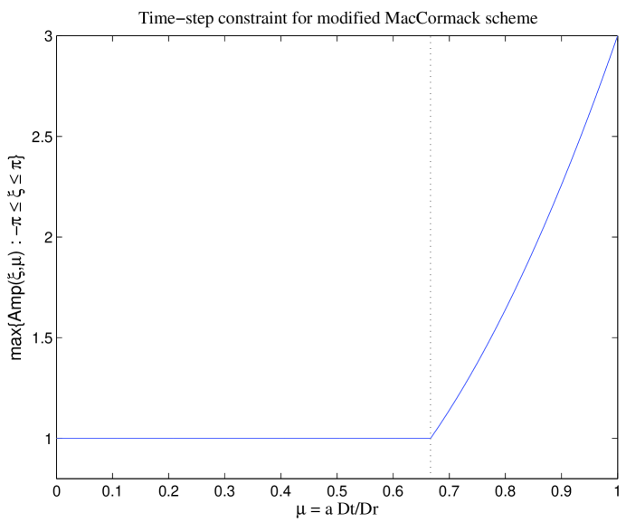
Figure 44. First output from the given matlab code.

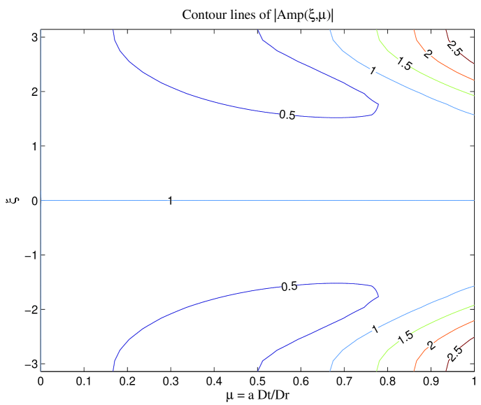
Figure 45. Second output from the given matlab code.

Since $F(U,U,U)=U$, the scheme is in consistent conservation form as applied to a conservation law like the $1+1$ flatspace advection equation [45]. Following Minion’s description [84] of a standard stability analysis, we have written a short matlab code (given below) which demonstrates that the modified scheme is stable for the time–step constraint $a\Delta t\big{/}\Delta r<2/3$ (or a number shockingly close to $2/3$). The output plots for this code are depicted in Figs. 44 and 45. The second plot shows that instability in the scheme stems from the highest modes.

For the straight interior MacCormack scheme as applied to the system (130) and (131) of evolution equations, we have remarked in Section 4.2.2 that we expect evolution stability for $\Delta t\big{/}\Delta r<1$. Recall that this is the expectation because the variable $X$ propagates everywhere with speed $1$, while $(\rho_{B}-1)/(\rho_{B}+1)<1$ is the maximum speed of $U$ over the domain $[2\mathrm{m},r_{B}]$, as is evident from (143). We now assume that our stability analysis for the modified MacCormack scheme —carried out using the model equation (189)— also pertains to (130). Since the modified scheme is only used at the outermost boundary point, we let $a=(\rho_{B}-1)/(\rho_{B}+1)$. Then for $\rho_{B}=15$, we get $a=14/16$, and in turn the constraint $\Delta t\big{/}\Delta r<16/21\simeq 0.7619$ associated with the modified scheme. Since the rhs of this constraint is less than $1$, the issue at hand is whether it is $16/21$ or $1$ which limits evolution stability. From numerical experiments, such as those in Section 5, we find that stability is ensured so long as $\Delta t\big{/}\Delta r<1$. Although the modified MacCormack time–step constraint is more restrictive, it is not a limitation for our numerical evolutions, presumably because the modified scheme is implemented only at a single point.

%
%  S R Lau
%  Applied Mathematics Group
%  Department of Mathematics
%  University of North Carolina
%  Chapel Hill, NC 27599-3250
%  USA
%
%  26 October 2003
%
%  Matlab code: ModifiedMacCormack.m
%
%  Code produces two plots, each of which elucidates the time-step
%  stability associated with applying a modified MacCormack scheme
%  to the 1+1 linear advection equation,
%
%  U_t + a U_r = 0,
%
%  where a > 0 is a constant velocity. Our method of analysis
%  follows M. L. Minion, "On the Stability of Godunov-Projection
%  Methods for Incompressible Flow," J. Comp. Phys. {\bf 123}, 435
%  (1996).
%
%  The modified MacCormack scheme is as follows. In terms of the
%  Courant-Friedrich-Levy factor
%
%  mu = a Dt/Dr,
%
%  we obtain the predicted variable
%
%  barU(n+1,q) = U(n,q)  - mu [U(n,q) - U(n,q-1)].             (A)
%
%  Next, we construct the corrected variable
%
%  tilU(n+1,q) = 0.5{barU(n+1,q) + U(n,q) - mu
%            [2barU(n+1,q) - 3barU(n+1,q-1) + barU(n+1,q-2)]}. (B)
%
%  The three terms within the square parenthesis correspond
%  to [barU(n+1,q+1) - barU(n+1,q)] in the straight MacCormack
%  scheme. However, here we use the extrapolation
%
%  3barU(n+1,q) - 3barU(n+1,q-1) + barU(n+1,q-2)
%
%  in place of barU(n+1,q+1). This scheme is inspired by how
%  ROBC have been implemented within the MacCormack scheme in
%  S  R  Lau, "Rapid Evaluation of Radiation Boundary Kernels for
%  Time-Domain Wave Propagation on Blackholes." UNC-Chapel Hill
%  Ph.D. dissertation (2003). See the end of Chapter 4.
%
%  To perform a standard Von Neumann stability analysis, suppose
%  that U is periodic on [0,2pi], and represented by the discrete
%  Fourier series
%
%           Q/2-1
%  U(j) =    Sum    hatU(p) exp(j p Dr),                       (C)
%          p = -Q/2
%
%  where Dr = 2pi/Q and hatU is the Fourier transform of U. Then
%  the range of xi = p Dr lies in [-pi,pi]. To define Amp(xi,mu),
%  the amplification factor, we substitute the spectral form (C)
%  into equations (A) and (B) above, in order to get the symbol
%  Amp for one step of the method:
%
%  hatU(n+1,p) = Amp(xi,mu) hatU(n,p).
%
%  Having given the relevant background, let us turn to the code.
%
%  Step 1. Build up a two-by-two mesh grid with CFL factor mu
%  along x-axis and angle xi = p Dr along y-axis. The argument
%  of each trigonometric function which makes up the amplification
%  factor Amp involves p Dr = 2 pi p/Q, so to test Amp we sample
%  xi from -pi to pi at regular intervals (continuity of Amp
%  ensures that we need not sample every xi).
%
%  Choose discretization sizes for mu and xi arrays, and build the
%  mesh grid.
%
Dmu = 0.001;
Dxi = pi/16;
[xi,mu] = meshgrid(-pi:Dxi:pi,0:Dmu:1);
%
%  Step 2. Build corresponding two-by-two array of values for
%  the Amp symbol particular to the modified MacCormack scheme.
%
Exp1  = exp(-i*xi);
Exp2  = exp(-2*i*xi);
Exp3  = exp(-3*i*xi);
term1 = 3-4*Exp1+Exp2;
term2 = 2-5*Exp1+4*Exp2-Exp3;
Amp   = 1-0.5*mu.*term1+0.5*mu.*mu.*term2;
%
%  Step 3. Make the first plot. For each point in the mu array,
%  we compute the maximum of |Amp(xi,mu)| over all xi. Note mu = 0
%  always gives an amplification factor of unity, so maxAmpMod > 1
%  marks instability.
%
[J K] = size(Amp);
for j = 1:J
maxAmpMod(j)  = max(abs(Amp(j,:)));
end
figure(1)
hold off
plot(mu(1:J,1),maxAmpMod)
hold on
xlabel(’\mu = a Dt/Dr’)
ylabel(’max\{Amp(\xi,\mu) : -\pi \leq \xi \leq \pi\}’)
title(’Time--step constraint for modified MacCormack scheme’)
plot((2/3)*ones(size([0.8:0.1:3])),[0.8:0.1:3],’k:’)
axis tight
%
%  Step 4. Make the second plot. Here we plot contour lines of
%  the modulus of the Amplification factor in order to see which
%  xi are the most amplified.
%
figure(2)
hold off
[CS H] = contour(mu,xi,abs(Amp));
xlabel(’\mu = a Dt/Dr’)
ylabel(’\xi’)
title(’Contour lines of |Amp(\xi,\mu)|’)
clabel(CS,H,’manual’)
%
%  Press "return" to exit manual labeling.
%

Appendix B Numerical Tables for Compressed Kernels

We list the pole locations $\beta_{n}$ and strengths $\gamma_{n}$ for a few compressed kernels used in the numerical tests of Section 5. A table entry of $0$ indicates an output number from the compression algorithm which is less than $10^{-30}$ in absolute value. For those $\beta_{n}$ and $\gamma_{n}$ appearing in conjugate pairs, we list only the one with positive imaginary part.

$n$	$\beta^{R}_{n}$	$\beta^{I}_{n}$
1	$-$0.407381913421500E+00	0
2	$-$0.292310786462780E+00	0
3	$-$0.212438334101443E+00	0
4	$-$0.154351731119108E+00	0
5	$-$0.111621522695175E+00	0
6	$-$0.801606769182339E$-$01	0
7	$-$0.570590618998134E$-$01	0
8	$-$0.401964994812843E$-$01	0
9	$-$0.280020468146328E$-$01	0
10	$-$0.192813689223556E$-$01	0
11	$-$0.131170606343391E$-$01	0
12	$-$0.881053984705117E$-$02	0
13	$-$0.583815623973656E$-$02	0
14	$-$0.381311155357965E$-$02	0
15	$-$0.245325710136527E$-$02	0
16	$-$0.155499824057403E$-$02	0
17	$-$0.970762744563191E$-$03	0
18	$-$0.585846647089220E$-$03	0
19	$-$0.373076210020314E$-$03	0
20	$-$0.183147313598350E$-$03	0

$n$	$\gamma^{R}_{n}$	$\gamma^{I}_{n}$
1	$-$0.560438492794723E$-$06	0
2	$-$0.149307319758660E$-$04	0
3	$-$0.100427245970089E$-$03	0
4	$-$0.294347741100713E$-$03	0
5	$-$0.482077412607607E$-$03	0
6	$-$0.512454401482300E$-$03	0
7	$-$0.391967225466562E$-$03	0
8	$-$0.233213890995425E$-$03	0
9	$-$0.114815532845651E$-$03	0
10	$-$0.490292206150649E$-$04	0
11	$-$0.187703451634142E$-$04	0
12	$-$0.658176657111368E$-$05	0
13	$-$0.214158551560558E$-$05	0
14	$-$0.651562115228849E$-$06	0
15	$-$0.186157771876132E$-$06	0
16	$-$0.501212404555003E$-$07	0
17	$-$0.128840007496407E$-$07	0
18	$-$0.314418019702290E$-$08	0
19	$-$0.569152368353698E$-$09	0
20	$-$0.244872495848780E$-$09	0

Table 13. Kernel for $\jmath=0$, $l=0$, $\rho_{B}=15$, $\varepsilon=10^{-10}$.

$n$	$\beta^{R}_{n}$	$\beta^{I}_{n}$
1	$-$0.347849789139467E+01	0
2	$-$0.328013420888283E+01	0.122459742396181E+01
3	$-$0.277834690894067E+01	0.221807916777226E+01
4	$-$0.216780239221729E+01	0.288987484597755E+01
5	$-$0.160611143055369E+01	0.328338093803925E+01
6	$-$0.116571976808040E+01	0.348766466680969E+01
7	$-$0.870203833982946E+00	0.359360642350047E+01
8	$-$0.654574374170026E+00	0.373250677729775E+01
9	$-$0.383775970479126E+00	0.391836743018780E+01

$n$	$\gamma^{R}_{n}$	$\gamma^{I}_{n}$
1	$-$0.351882332982489E+02	0
2	$-$0.288247787077508E+02	0.145963809805392E+02
3	$-$0.159408675098397E+02	0.197009045186916E+02
4	$-$0.579079784769916E+01	0.165503367808947E+02
5	$-$0.888910445944541E+00	0.110514097610705E+02
6	+0.617612362898097E+00	0.649132105745073E+01
7	+0.488858645232752E$-$01	0.363187756402738E+01
8	$-$0.604551383223953E+00	0.358904868249248E+01
9	$-$0.352475685403885E+00	0.379107013210578E+01

Table 14. Kernel for $\jmath=2$, $l=64$, $\rho_{B}=15$, $\varepsilon=10^{-10}$. Complex conjugation of entries 2–9 gives entries 10–17.

$n$	$\beta^{R}_{n}$	$\beta^{I}_{n}$
1	$-$0.375616176922446E+00	0
2	$-$0.252285897920276E+00	0
3	$-$0.171458781191188E+00	0
4	$-$0.116562490243471E+00	0
5	$-$0.764331990276028E$-$01	0
6	$-$0.468091057981411E$-$01	0
7	$-$0.263730137927373E$-$01	0
8	$-$0.125652994567027E$-$01	0
9	$-$0.947795178946719E$-$01	0.599312024947409E$-$01

$n$	$\gamma^{R}_{n}$	$\gamma^{I}_{n}$
1	$-$0.942815440763951E$-$05	0
2	$-$0.366046310052021E$-$03	0
3	$-$0.374027383588918E$-$02	0
4	$-$0.872734265927278E$-$02	0
5	$-$0.147189136342128E$-$02	0
6	$-$0.501356988668342E$-$04	0
7	$-$0.973423621068051E$-$06	0
8	$-$0.728807025058112E$-$08	0
9	$-$0.894836172990982E$-$01	0.620643548936884E$-$01

Table 15. Kernel for $\jmath=2$, $l=2$, $\rho_{B}=15$, $\varepsilon=10^{-10}$. Complex conjugation of entry 9 gives entry 10.

References

- [1] S. R. Lau, Rapid Evaluation of Radiation Boundary Kernels for Time–domain Wave Propagation on Blackholes, applied math Ph.D dissertation, UNC–Chapel Hill, December 2003.
- [2] J. D. Brown and J. W. York, Quasilocal energy and conserved charges derived from the gravitational action, Phys. Rev. D 47, 1407 (1993).
- [3] J. D. Brown, S. R. Lau, and J. W. York, Action and energy of the gravitational field, Ann. Phys. 297, 175 (2002).
- [4] E. Lindman, Free space boundary conditions for the time dependent wave equation, J. Comp. Phys. 18, 66 (1975).
- [5] B. Engquist and A. Majda, Absorbing boundary conditions for the numerical simulation of waves, Math. Comp. 31, 629 (1977).
- [6] B. Engquist and A. Majda, Radiation boundary conditions for acoustic and elastic wave calculations, Comm. Pure Appl. Math. 32, 313 (1979).
- [7] B. Gustafsson and H.–O. Kreiss, Boundary conditions for time–dependent problems with an artificial boundary, J. Comp. Phys. 30, 333 (1979).
- [8] A. Bayliss and E. Turkel, Radiation boundary conditions for wave–like equations, Comm. Pure Appl. Math. 33, 707 (1980).
- [9] T. Hagstrom, Reduction of Unbounded Domains to Bounded Domains for Partial Differential Equation Problems, Ph.D. dissertation, California Institute of Technology (1983).
- [10] R. Kosleff and D. Kosleff, Absorbing boundaries for wave propagation problems, J. Comp. Phys. 63, 363 (1986).
- [11] D. Givoli, Non–reflecting boundary conditions, J. Comp. Phys. 94, 1 (1991).
- [12] I. L. Sofronov, Conditions for complete transparency on the sphere for the three–dimensional wave equation, Russian Acad. Sci. Dokl. Math. 46, No. 2, 397 (1993).
- [13] J.-P. Berenger, A perfectly matched layer for the absorption of electromagnetic waves, J. Comp. Phys. 114, 185 (1994).
- [14] M. J. Grote and J. B. Keller, On nonreflecting boundary conditions, J. Comp. Phys. 122, 231 (1995).
- [15] M. J. Grote and J. B. Keller, Exact nonreflecting boundary conditions for the time dependent wave equation, SIAM J. Appl. Math. 55, No. 2, 280 (1995).
- [16] M. J. Grote and J. B. Keller, Nonreflecting boundary conditions for time–dependent scattering, J. Comp. Phys. 127, 52 (1996).
- [17] T. Hagstrom, Radiation boundary conditions for the numerical simulation of waves, Acta Numerica 8, 47 (1999).
- [18] B. Alpert, L. Greengard, and T. Hagstrom, Rapid evaluation of nonreflecting boundary kernels for time–domain wave propagation, SIAM J. Numer. Anal. 37, 1138 (2000).
- [19] B. Alpert, L. Greengard, and T. Hagstrom, Nonreflecting boundary conditions for the time–dependent wave equation, J. Comp. Phys. 180, 270 (2002).
- [20] T. Hagstrom, New Results on Absorbing Layers and Radiation Boundary Conditions, in Topics in Computational Wave Propagation, edited by M. Ainsworth, P. Davies, D. Duncan, P. Martin, and B. Rynne (Springer–Verlag, New York, 2003).
- [21] G. N. Watson, A Treatise on the Theory of Bessel Functions, second edition (Cambridge University Press, Cambridge, 1944).
- [22] F. G. Friedlander, On the radiation field of pulse solutions of the wave equation, Proc. Roy. Soc. A 269, 53 (1962).
- [23] J. A. Wheeler, Geons, Phys. Rev. 97, 511 (1955).
- [24] T. Regge and J. A. Wheeler, Stability of a Schwarzschild singularity, Phys. Rev. 108, 1063 (1957).
- [25] F. J. Zerilli, Gravitational field of a particle falling in a Schwarzschild geometry analyzed in tensor harmonics, Phys. Rev. D 2, 2141 (1970).
- [26] S. Chandrasekhar, Mathematical Theory of Black Holes, (Oxford University Press, Oxford, 1992).
- [27] J. W. York, Jr., Kinematics and dynamics of general relativity, in Sources of Gravitational Radiation, edited by L. L. Smarr (Cambridge University Press, Cambridge, 1979).
- [28] H. Friedrich and G. Nagy, Comm. Math. Phys. 201, 619 (1999).
- [29] N. T. Bishop, R. Gómez, L. Lehner, and J. Winicour, Cauchy–characteristic extraction in numerical relativity, Phys. Rev. D 54, 6153 (1996).
- [30] N. T. Bishop, R. Gómez, L. Lehner, M. Maharaj, and J. Winicour, High–powered gravitational news, Phys. Rev. D 56, 6298 (1997).
- [31] M. E. Rupright, A. M. Abrahams, and, L. Rezzolla, Cauchy–perturbative matching and outer boundary conditions I: Methods and tests, Phys. Rev. D 58, 044005 (1998).
- [32] L. Rezzolla, A. M. Abrahams, R. A. Matzner, M. E. Rupright, and S. L. Shapiro, Cauchy–perturbative matching and outer boundary conditions: Computational studies, Phys. Rev. D 59, 064001 (1999).
- [33] S. R. Lau, Outer boundary as arrested history in general relativity, Class. Quantum Grav. 19, 2853 (2002); Corrigendum, Class. Quantum Grav. 20, 1415 (2003).
- [34] B. Szilágyi, B. Schmidt, J. Winicour, Boundary conditions in linearized harmonic gravity, Phys. Rev. D 65 064015 (2002).
- [35] J. Novak and S. Bonazzola, Solving wave equations with spectral methods and nonreflecting boundary conditions, gr-qc/0203102.
- [36] E. W. Allen, E. Buckmiller, L. M. Burko, and R. H. Price, Radiation tails and boundary conditions for black hole evolutions, gr-qc/0401092.
- [37] G. B. Cook and S. A. Teukolsky, Numerical relativity: challenges for computational science, Acta Numerica 8, 1 (1999).
- [38] E. W. Leaver, Spectral decomposition of the perturbation response of the Schwarzschild geometry, Phys. Rev. D 34, 384 (1986).
- [39] N. Andersson, Evolving test fields in a black–hole geometry, Phys. Rev. D 55, 468 (1997).
- [40] P. M. Morse and H. Feshbach, Methods of Theoretical Physics, vols. 1 and 2 (McGraw–Hill Book Company, Inc., New York, 1953).
- [41] Heun’s Differential Equations, edited by A. Ronveaux (Oxford University Press, Oxford, 1995).
- [42] S. Y. Slavyanov and W. Lay, Special Functions: a Unified Theory Based on Singularities (Oxford University Press, Oxford, 2000).
- [43] A. H. Wilson, A generalized spheroidal wave equation, Proc. R. Soc. Lon. A 118, 617 (1928).
- [44] E. W. Leaver, Solutions to a generalized spheroidal wave equation: Teukolsky’s equation in general relativity, and the two–center problem in molecular quantum mechanics, J. Math. Phys. 27, 1238 (1986).
- [45] R. J. LeVeque, Numerical Methods for Conservation Laws, second edition (Birkhäuser Verlag, Basel, 1992).
- [46] B. Gustafsson, The convergence rate for difference approximations to mixed initial boundary value problems, Math. Comp. 29, 396 (1975).
- [47] R. J. LeVeque and J. Oliger, Numerical methods based on additive splittings for hyperbolic partial differential equations, J. Comp. Phys. 40, 469 (1983).
- [48] J. M. Sans–Serna, J. G. Verwer, and W. H. Hundsdorfer, Convergence and order reduction of Runge-Kutta schemes applied to evolutionary problems in partial differential equations, Numer. Math. 50 405 (1986).
- [49] M. H. Carpenter, D. Gottlieb, S. Abarbanel and W.–S. Don, The theoretical accuracy of Runge-Kutta time discretization for the initial boundary value problem: a study of the boundary error, SIAM J. Sci. Comp. 16, 1241 (1995).
- [50] S. Abarbanel, D. Gottlieb, and M. H. Carpenter, On the removal of boundary errors caused by Runge-Kutta integration of nonlinear partial differential equations, SIAM J. Sci. Comp. 17, 777 (1996).
- [51] D. Pathria, The correct formulation of intermediate boundary conditions for Runge-Kutta time integration of initial boundary value problems, SIAM J. Sci. Comp. 18, 1255 (1997).
- [52] C. W. Misner, K. S. Thorne, and J. A. Wheeler, Gravitation (Freeman, San Francisco, 1973).
- [53] M. E. Taylor, Partial Differential Equations, vol. 3 (Springer–Verlag, New York, 1997).
- [54] P. K. Chattopadhyay, Mathematical Physics (New Age International, Ltd., New Delhi, 1990).
- [55] M. D. Greenberg, Advanced Engineering Mathematics (Prentice–Hall, Inc., Englewood Cliffs, 1988).
- [56] J. J. Duistermatt and F. A. Grünbaum, Differential equations in the spectral parameter, Comm. Math. Phys. 103, 177 (1986).
- [57] C. M. Bender and S. A. Orszag, Advanced Mathematical Methods for Scientists and Engineers, (McGraw–Hill Book Company, Inc., New York, 1978).
- [58] L. J. Slater, Confluent hypergeometric functions (Cambridge University Press, Cambridge, 1960).
- [59] A. R. Curtis, Coulomb Wave Functions, Royal Soc. Math. Tables, vol. 11 (Cambridge University Press, Cambridge, 1964).
- [60] I. J. Thompson and A. R. Barnett, Coulomb and Bessel functions of complex arguments and order, J. Comp. Phys. 64, 490 (1986).
- [61] Olver, F. W. J. Asymptotics and Special Functions (Academic Press, New York and London, 1974).
- [62] K. E. Atkinson, Elementary Numerical Analysis, second edition (Wiley, New York, 1993).
- [63] S. Jiang, Fast Evaluation of Nonreflecting Boundary Conditions for the Schrödinger Equation, New York University Ph.D. Dissertation (2001).
- [64] K. S. Thorne, Multipole expansions of gravitational radiation, Rev. Mod. Phys. 52, 299 (1980).
- [65] H.–P. Nollert and B. G. Schmidt, Quasinormal modes of Schwarzschild black holes: Defined and calculated via Laplace transformation, Phys. Rev. D 45, 2617 (1992).
- [66] H. S. Wall, Analytic Theory of Continued Fractions (D. Van Nostrand Co., New York, 1948).
- [67] C. R. Evans and S. R. Lau, in preparation, Fall 2004.
- [68] K. D. Kokkotas and B. G. Schmidt, Quasi–Normal Modes of Stars and Black Holes, Living Reviews of Relativity 2, 2, and gr–qc/9909058.
- [69] B. F. Schutz, Gravitational wave astronomy, Class. Quantum Grav. 16, A131 (1999).
- [70] L. Blanchet, On the multipole expansion of the gravitational field, Class. Quantum Grav. 15, 1971 (1998).
- [71] C. T. Cunningham, R. H. Price, and V. Moncrief, Radiation from collapsing relativistic stars. I. Linearized odd–parity radiation, Ap. J. 224, 643 (1978).
- [72] V. Moncrief, C. T. Cunningham, and R. H. Price, Radiation from slightly nonspherical models of collapse, in Sources of Gravitational Radiation, edited by L. L. Smarr (Cambridge University Press, Cambridge, 1979).
- [73] N. Andersson, K. D. Kokkotas, and B. F. Schutz, A new numerical approach to the oscillation modes of relativistic stars, Mon. Not. Roy. Astron. Soc. 274, 1039 (1995).
- [74] N. Andersson, K. D. Kokkotas, and B. F. Schutz, Spacetime modes of relativistic stars, Mon. Not. Roy. Astron. Soc. 280, 1230 (1996).
- [75] G. Allen, N. Andersson, K. D. Kokkotas, B. F. Schutz, Gravitational waves from pulsating stars: Evolving the perturbation equations for a relativistic star, Phys. Rev. D 58, 124012 (1998).
- [76] B. P. Sinha and R. H. MacPhie, On the computation of the prolate spheroidal radial functions of the second kind, J. Math. Phys. 16, 2378 (1975).
- [77] L.–W. Li, X.–K. Kang, and M.–S. Leong, Spheroidal Wave Functions in Electromagnetic Theory (Wiley, New York, 2002).
- [78] B. Alpert, L. Greengard, and T. Hagstrom, An integral evolution formula for the wave equation, J. Comp. Phys. 162, 536 (2000).
- [79] W. Kress, A compact fourth order time discretization method for the wave equation, Technical Report 2003-041, Dept. of Information Technology, Uppsala University.
- [80] W. Kress and B. Gustafsson, Deferred correction methods for initial boundary value problems, J. Sci. Comp. 17, 241 (2002).
- [81] M. L. Minion, Semi–implicit spectral deferred correction methods for ordinary differential equations, Comm. Math. Sci. 1, 471 (2003).
- [82] S. Rosenberg, The Laplacian on a Riemannian Manifold (Cambridge University Press, Cambridge, 1997).
- [83] S. W. Hawking and G. F. R. Ellis, The Large Scale Structure of Space–time (Cambridge University Press, Cambridge, 1973).
- [84] M. L. Minion, On the stability of Godunov–projection methods for incompressible flow, J. Comp. Phys. 123, 435 (1996).