A Post-Newtonian diagnostic of quasi-equilibrium binary configurations of compact objects

Abstract

Using equations of motion accurate to the third post-Newtonian (3PN) order ($O(v/c)^{6}$ beyond Newtonian gravity), we derive expressions for the total energy $E$ and angular momentum $J$ of the orbits of compact binary systems (black holes or neutron stars) for arbitrary orbital eccentricity. We also incorporate finite-size contributions such as spin-orbit and spin-spin coupling, and rotational and tidal distortions, calculated to the lowest order of approximation, but we exclude the effects of gravitational radiation damping. We describe how these formulae may be used as an accurate diagnostic of the physical content of quasi-equilibrium configurations of compact binary systems of black holes and neutron stars generated using numerical relativity. As an example, we show that quasi-equilibrium configurations of corotating neutron stars recently reported by Miller et al. can be fit by our diagnostic to better than one per cent with a circular orbit and with physically reasonable tidal coefficients.

I Introduction and Summary

The late stage of inspiral of binary systems of neutron stars or black holes is of great current interest, both as a challenge for numerical relativity, and as a possible source of gravitational waves detectable by laser interferometric antennas. Because this stage, corresponding to the final few orbits and ultimate merger of the two objects into one, is highly dynamical and involves strong gravitational fields, it must be handled by numerical relativity, which attempts to solve the full Einstein equations on computers (see Refs. cook ; seidel ; baumshapiro for reviews).

The early stage of inspiral can be handled accurately using post-Newtonian techniques, which involve an expansion of solutions of Einstein’s equations in powers of $\epsilon\sim(v/c)^{2}\sim Gm/rc^{2}$, where $v$, $m$, and $r$ are the typical velocity, mass and separation in the system, respectively. By expanding to very high powers of $\epsilon$, one can derive increasingly accurate formulae to describe both the orbital motion and the gravitational waveform. Currently, results for the orbital motion accurate through 3.5PN order ($O(\epsilon^{7/2})$ beyond Newtonian gravity) are known jaraschafer98 ; jaraschafer99 ; djs00 ; djs01 ; bf00 ; bf01 ; abf01 ; bdgef03 ; futamase01 ; itohfuta03 ; dire2 .

An important issue in understanding the full inspiral of compact binaries is how to connect the PN regime to the numerical regime. This is a non-trivial issue because the PN approximation gets worse the smaller the separation between the bodies. On the other hand, because of limited computational resources, numerical simulations cannot always be started with separations sufficiently large to overlap the PN regime where it is believed to be reliable. This has given rise to the so-called Intermediate Binary Black Hole (IBBH) problem ibbh , for example, which seeks new techniques or insights to attempt to bridge the gap between the end of confidence in PN methods and the beginning of realistic numerical simulations. On the other hand, if it can be demonstrated that PN approximations converge sufficiently rapidly, especially for comparable-mass binary systems, then IBBH techniques may not be needed. Blanchet luc02 ; luchopkins has recently argued that, for comparable-mass systems, the PN approximation seems to be more accurate than might be expected based on experience with the test-body limit. For binary neutron stars, this is less of an issue, because neutron stars are much larger objects, so the numerical simulations necessarily commence at larger separations, where PN methods are presumably more reliable.

Numerical simulations of compact binary inspiral start with a solution of the initial value equations of Einstein’s theory; these provide the initial data for the evolution equations (some initial-data models ggb02 solve in addition one of the six dynamical field equations). The initial state is assumed to consist of two compact objects (neutron stars or black holes) in an initially circular orbit. For stellar-mass systems that have evolved in isolation for eons, gravitational radiation is expected to leave the orbit in an accurately circular state, apart from the adiabatic inspiral induced by the loss of orbital energy; that inspiral is ignored in the initial-data models. (Miller has analysed the consequences of this particular assumption miller03 ).

The circular-orbit condition is imposed by demanding that $dr/dt=0$ initially, where $r$ is a measure of the orbital separation. One way to achieve this is to require that the system have an initial “helical Killing vector” (HKV), which corresponds to a kind of rigid rotation of the binary system. Some initial-data models assume that the objects are co-rotating, a condition which is astrophysically unlikely, albeit computationally advantageous, while others assume that the bodies are irrotational, i.e. non-rotating in an inertial frame. To simplify the problem, an approximation for the spatial metric is generally made; one is the assumption of conformal flatness, an approximation that is known to be invalid in full general relativity. This approximation is usually justified by the neglect of radiation reaction in the initial state. Other approximations, derived from post-Newtonian theory, or from sums of Kerr geometries, have also been used. For black hole binaries, suitable horizon boundary conditions must be imposed, while for neutron star binaries, equations of hydrostationary equilibrium and an equation of state must be provided.

One important product of these initial value solutions is a relationship between the energy $E$ and angular momentum $J$ of the system as measured at infinity, and the orbital frequency $\Omega$. The energy could be the total energy as measured at infinity, consisting of the masses of the two stars plus the orbital energy, or it could be the total energy less the energy of the same two stars in isolation. The latter quantity would be a measure of the orbital binding energy. As all quantities are well-defined and gauge invariant, they are useful variables for making comparisons with PN methods.

We have developed formulae for $E(\Omega)$ and $J(\Omega)$ using PN methods. Our analytic formulae include point-mass terms through 3PN order, but ignore radiation reaction. They also include rotational energy and spin-orbit and spin-spin terms for the case in which the bodies are rotating. They further include a Newtonian calculation of the effects of tidal and rotational distortions, applicable to stars of arbitrary density distribution, expressed in terms of so-called “apsidal constants” (i.e. we do not restrict attention to homogeneous ellipsoids wisemanlai ), and including effects at quadrupole and octupole order. We verify that, for black holes, tidal effects can be ignored, while for neutron-star binaries, they must be included. In contrast to previous work luc02 ; cook94 ; pfeiffer ; dgg02 , our formulae apply to general eccentric orbits, not just to circular orbits.

In an earlier paper morawill , we compared this formula with HKV numerical solutions for corotating binary black holes obtained by Grandclément et al. ggb02 , for the regime where the black holes are separated from the location of the innermost circular orbit by a factor of around two, where PN results might be expected to work well ($Gm/rc^{2}\sim 0.1$). We found that when we assumed circular PN orbits, our 3PN formulae for $E(\Omega)$ and $J(\Omega)$ agreed to within 0.5 % with other PN methods, including our own formulae truncated at 2PN order, and 3PN formulae derived using resummation or Padé techniques. However all PN methods consistently and systematically underestimated the binding energy and overestimated the angular momentum, compared to the values derived from the numerical HKV initial-data models, by amounts that were up to 10 times larger than the spread among the PN methods. But when we relaxed the assumption of a circular orbit and demanded only that $dr/dt=0$, our PN formula could be made to agree extremely well with the numerical data by assuming that the system being simulated is initially at the apocenter of a slightly eccentric orbit. For values of $Gm\Omega/c^{3}$ ranging from 0.03 to 0.06, corresponding to orbital $v/c$ between 0.3 and 0.4, or orbital separation between 10 and 6 $Gm/c^{2}$, nearly perfect agreement with the binding energy and the angular momentum could be obtained with eccentricities that range from 0.03 to 0.05.

The concordance within fractions of a percent between the various 2PN, 3PN and resummation PN results matches expectation, since $(Gm/rc^{2})^{3}\sim 10^{-3}$. Presuming that all relevant physical effects have been included, we argued that the PN results in this range of $Gm\Omega/c^{3}$ are robust. We suggested the possibility that the approximations made in most numerical initial-data models could lead to an apparent eccentricity in what was expected to be a quasi-circular orbit. At present, however, the discrepancy between the two approaches can only be considered a hint of possible eccentricity, because the results of ggb02 did not include quantitative error bars for the variables $E(\Omega)$ and $J(\Omega)$.

These results motivate us to propose a “post-Newtonian diagnostic”, a tool that can be used to extract physical information from numerical simulations, and that may also be an aid to guide some of the assumptions and approximations inherent in numerical initial data computations toward those that lead to the desired physical configuration, such as a true quasi-circular orbit.

In this paper we provide the physical assumptions, mathematical details, and justifications for the approximations that underly this proposed diagnostic tool. We give the detailed foundations for the analysis carried out in morawill for black-hole binary systems, and also extend that work to the case of neutron-star systems by including tidal effects. As an application of our diagnostic to neutron-star systems, we analyse recent numerical models of quasi-equilibrium orbits of neutron stars by Miller et al. mgs03 . In contrast to the black-hole case, we find that the orbital energy in the neutron-star initial-data models of mgs03 can be fit to better than one percent, and importantly, within the error bars provided in mgs03 , using circular orbits with physically reasonable tidal parameters appropriate to the “$\Gamma=2$” equation of state used in that numerical work. The results illustrate the robustness of the PN approximation well into the strongly relativistic regime of compact binaries, especially when augmented with physically movitated finite-size effects. Application of this PN diagnostic to other numerical models will be subject of future papers.

The remainder of this paper provides the details underlying these conclusions. In Sec. II, we solve the post-Newtonian equations of motion calculated to third post-Newtonian (3PN) order, for general eccentric orbits. Neglecting radiation reaction effects, we then express the total conserved orbital energy and angular momentum in terms of a pair of “covariant” orbit elements $e$ (eccentricity) and $\zeta$ (related to the semi-latus rectum). In Sec. III, we calculate the effects of finite size in binary systems with bodies whose spin axes are perpendicular to the orbital plane. These include tidal and rotational distortions, spin-orbit terms and spin-spin terms. In Sec. IV, we analyse our diagnostic quantitatively, and apply it to co-rotating, equal-mass binaries of black holes and of neutron stars. Two appendices provide the detailed derivations of the expressions for the tidal and rotational distortion included in our diagnostic: Appendix A uses Newtonian gravity to solve the general problem of the equilibrium configurations of gravitating bodies disturbed by an external force, paralleling the treatment in the classic monographs of Kopal kopal1 ; kopal2 , and Appendix B specializes the results to linear perturbations caused by rotational and tidal disturbances.

II Energy and angular momentum for “point” masses to 3PN order

II.1 Orbits at the turning point in post-Newtonian gravity

Since our ultimate focus will be on orbits that are possibly eccentric, but that momentarily have $\dot{r}=0$, it will be useful to review the characteristics of orbits at turning points in Newtonian theory. In Newtonian gravity, the orbit of a pair of point masses may be described by the set of equations

$$p/r = 1+e\cos(\phi-\omega)\,,$$

$$r^{2}\Omega \equiv r^{2}d\phi/dt=(mp)^{1/2}\,,$$

$$E = \mu({\dot{r}}^{2}+r^{2}\Omega^{2})/2-\mu m/r\,,$$

$$J = \mu|{\bf x}\times{\bf v}|\,,$$ (1)

where $p=a(1-e^{2})$ is the semi-latus rectum ($a$ is the semi-major axis), $\omega$ is the angle of pericenter, $m=m_{1}+m_{2}$ is the total mass, $\mu=m_{1}m_{2}/m$ is the reduced mass, and $E$ and $J$ are the total orbital energy and angular momentum, respectively (henceforth we use units in which $G=c=1$). A circular orbit corresponds to $e=0$, with $r=a=$ constant, $\Omega^{2}=m/a^{3}$, $E/\mu=a^{2}\Omega^{2}/2-m/a=-(m\Omega)^{2/3}/2$, and $J/\mu=\sqrt{ma}=(m/\Omega)^{1/3}$. However, if we demand only that the orbit be at apocenter, so that $\dot{r}=0$ only, we have $\phi=\omega+\pi$, $r=p/(1-e)$, $\Omega^{2}=(m/p^{3})(1-e)^{4}$, so that, in terms of $\Omega_{a}$, the angular velocity at apocenter,

$$E/\mu = -\frac{1}{2}(1-e^{2})\left[\frac{m\Omega_{a}}{(1-e)^{2}}\right]^{2/3}\,,$$

$$J/\mu m = \left[\frac{m\Omega_{a}}{(1-e)^{2}}\right]^{-1/3}.$$ (2)

To obtain expressions in terms of $\Omega_{p}$, the angular velocity at pericenter, one makes the replacements $\Omega_{a}\to\Omega_{p}$ and $e\to-e$ in Eqs. (2).

However, at higher PN orders, neither the orbital eccentricity ${e}$ nor the semi-latus rectum ${p}$ is uniquely or invariantly defined. One definition of eccentricity used by Lincoln and Will lincwill in their analysis of orbits at 2.5PN order was that of a Newtonian orbit momentarily tangent to the true orbit (the “osculating” eccentricity); it had the unusual property that it did not tend to zero for a circular PN orbit, but tended toward a constant value of order $m/p$, while the rate of pericenter advance approached the same rate of rotation as the orbit itself. In this language, the true orbit was a non-circular orbit at perpetual periastron, thereby maintaining a constant separation $r$. In an effort to avoid this anomaly, other authors ds88 adopted a “quasi-Keplerian” parametrization, which defined multiple “eccentricities” to encapsulate different aspects of non-circular orbits at PN order.

In an effort to find a parametrization of non-circular PN orbits that will be useful in comparing with numerical models, we morawill proposed an alternative measure of eccentricity and semi-latus rectum according to:

$$e \equiv \frac{\sqrt{\Omega_{p}}-\sqrt{\Omega_{a}}}{\sqrt{\Omega_{p}}+\sqrt{\Omega_{a}}}\,,$$

$$\zeta\equiv\frac{m}{p} \equiv \left(\frac{\sqrt{m\Omega_{p}}+\sqrt{m\Omega_{a}}}{2}\right)^{4/3}\,,$$ (3)

where $\Omega_{p}$ is the value of $\Omega$ where it passes through a local maximum (pericenter), and $\Omega_{a}$ is the value of $\Omega$ where it passes through the next local minimum (apocenter).

These definitions have the following virtues: (1) they reduce precisely to the normal eccentricity $e$ and semi-latus rectum $p$ in the Newtonian limit, as can be verified from Eqs. (1); (2) they are constant in the absence of radiation reaction; (3) they are somewhat more directly connected to measurable quantities, since $\Omega$ is the angular velocity as seen from infinity (eg. as measured in the gravitational-wave signal) and one calculates only maximum and minimum values, without concern for the coordinate location in the orbit; and (4) they are straightforward to calculate in a numerical model of orbits without resorting to complicated definitions of “distance” between bodies.

They have the defect that, when radiation reaction is included, they are not local, continuously evolving variables, but rather are some kind of orbit-averaged quantities (for this reason, they may not be as “covariant” as they seem – see Sec. II.5 below). Nevertheless, when an eccentric orbit decays and circularizes under radiation reaction the definition of $e$ has the virtue that it tends naturally to zero when the orbital frequency turns from ocillatory behavior to monotonically increasing behavior (i.e. the maxima and minima merge).

By virtue of these definitions, $\zeta$ has the further property that

$$\zeta=\left(\frac{m\Omega_{p}}{(1+e)^{2}}\right)^{2/3}=\left(\frac{m\Omega_{a}}{(1-e)^{2}}\right)^{2/3}\,.$$ (4)

We will derive expressions for orbital energy and angular momentum in terms of these parameters $e$ and $\zeta$; for comparision with numerical models of quasi-equilibrium parametrized in terms of $\Omega$ at $\dot{r}=0$ ($\Omega_{a}$ or $\Omega_{p}$), one can simply substitute for $\zeta$ from Eq. (4). In this section we will focus on 3PN expressions for point masses; in the next section, we will incorporate effects due to rotation and finite size.

II.2 3PN equations of motion

We use the standard form of the equations of motion, written in a “Newtonian-like” manner. The acceleration of body 1 is given schematically by

$$\mathbf{a}_{1}=\frac{d^{2}\mathbf{x}_{1}}{dt^{2}} = \frac{m_{2}}{r^{2}}\left\{\mathbf{n}[-1+(PN)+(2PN)+(2.5PN)\right.$$ (5)

$$\left.\qquad+(3PN)+(3.5PN)+\cdots]\right.$$

$$\left.\qquad+\mathbf{v}[(PN)+(2PN)+(2.5PN)\right.$$

$$\left.\qquad+(3PN)+(3.5PN)+\cdots]\right\},$$

where $\mathbf{x}_{a}$ and $m_{a}$ denote the position and the mass of the body $a$, $r$ is the separation between the two bodies, $\mathbf{n}=(\mathbf{x}_{1}-\mathbf{x}_{2})/r$ is the unit vector from 2 to 1, and $\mathbf{v}=\mathbf{v}_{1}-\mathbf{v}_{2}$ the relative velocity. The equation for body 2 is obtained by making the replacement $1\rightleftharpoons 2$. The notation $nPN$ represents the $n^{th}$ post-Newtonian correction to Newtonian gravity. These equations are valid only for point-like, non-spinning bodies.

Post-Newtonian terms $nPN$ include even (integer) and odd (half-odd integer, such as 2.5PN, or 5/2 PN) orders. Even terms are conservative, in the sense that the equations of motion admit conserved quantities such as energy and angular momentum. Odd terms correspond to gravitational radiation reaction, and therefore are not conservative. In particular, they will cause the orbit to shrink, and the eccentricity to decrease.

We convert the two-body problem to an effective one-body problem. For this purpose we choose the origin to be at the center of mass of the system, which is defined by an integral of the motion (a conserved quantity to the 3PN order of approximation to which we will be working). We then change all variables to the relative coordinates $\mathbf{x}=\mathbf{x}_{1}-\mathbf{x}_{2}$ using relations of the type

$$\mathbf{x}_{1} = [m_{2}/m+(\eta\delta m/2m)(v^{2}-m/r)+(2PN)+\cdots]\mathbf{x}\,,$$

$$\mathbf{x}_{2} = [-m_{1}/m+(\eta\delta m/2m)(v^{2}-m/r)+(2PN)+\cdots]\mathbf{x}\,,$$ (6)

where $\eta=\mu/m=m_{1}m_{2}/m^{2}$ is the reduced mass parameter ($0<\eta\leq 1/4$), and $\delta m=m_{1}-m_{2}$. The result is a set of equations of motion in terms of relative coordinates:

$$\mathbf{a}=\frac{d^{2}\mathbf{x}}{dt^{2}}=\frac{m}{r^{2}}\left[(-1+A)\mathbf{n}+B\mathbf{v}\right]\,,$$ (7)

where $A$ and $B$ represent post-Newtonian terms. To date, the two-body equations of motion have been computed up to and including 3.5PN order. In an appropriate harmonic gauge, writing $A=A_{1}+A_{2}+\cdots$ and $B=B_{1}+B_{2}+\cdots$, the expressions for $A$ and $B$ read blanchetiyer03 :

$$A_{1} = 2(2+\eta)\frac{m}{r}-(1+3\eta)v^{2}+\frac{3}{2}\eta{\dot{r}}^{2}\,,$$ (8a)

$$A_{2} = -\frac{3}{4}(12+29\eta){\left(\frac{m}{r}\right)}^{2}-\eta(3-4\eta)v^{4}-\frac{15}{8}\eta(1-3\eta){\dot{r}}^{4}+\frac{1}{2}\eta(13-4\eta)\frac{m}{r}v^{2}$$ (8b)

$$+(2+25\eta+2\eta^{2})\frac{m}{r}{\dot{r}}^{2}+\frac{3}{2}\eta(3-4\eta)v^{2}{\dot{r}}^{2}\,,$$

$$A_{5/2} = \frac{8}{5}\eta\frac{m}{r}\dot{r}\left(\frac{17}{3}\frac{m}{r}+3v^{2}\right)\,,$$ (8c)

$$A_{3} = \left[16+\left(\frac{1399}{12}-\frac{41}{16}\pi^{2}\right)\eta+\frac{71}{2}\eta^{2}\right]{\left(\frac{m}{r}\right)}^{3}+\eta\left[\frac{20827}{840}+\frac{123}{64}\pi^{2}-\eta^{2}\right]{\left(\frac{m}{r}\right)}^{2}v^{2}$$ (8d)

$$-\left[1+\left(\frac{22717}{168}+\frac{615}{64}\pi^{2}\right)\eta+\frac{11}{8}\eta^{2}-7\eta^{3}\right]{\left(\frac{m}{r}\right)}^{2}{\dot{r}}^{2}$$

$$-\frac{1}{4}\eta(11-49\eta+52\eta^{2})v^{6}+\frac{35}{16}\eta(1-5\eta+5\eta^{2}){\dot{r}}^{6}-\frac{1}{4}\eta\left(75+32\eta-40\eta^{2}\right)\frac{m}{r}v^{4}$$

$$-\frac{1}{2}\eta\left(158-69\eta-60\eta^{2}\right)\frac{m}{r}{\dot{r}}^{4}+\eta\left(121-16\eta-20\eta^{2}\right)\frac{m}{r}v^{2}{\dot{r}}^{2}$$

$$+\frac{3}{8}\eta\left(20-79\eta+60\eta^{2}\right)v^{4}{\dot{r}}^{2}-\frac{15}{8}\eta\left(4-18\eta+17\eta^{2}\right)v^{2}{\dot{r}}^{4}\,,$$

$$A_{7/2} = -\frac{8}{5}\eta\frac{m}{r}\dot{r}\left[\frac{23}{14}(43+14\eta){\left(\frac{m}{r}\right)}^{2}+\frac{3}{28}(61+70\eta)v^{4}+70{\dot{r}}^{4}\right.$$ (8e)

$$\left.+\frac{1}{42}(519-1267\eta)\frac{m}{r}v^{2}+\frac{1}{4}(147+188\eta)\frac{m}{r}{\dot{r}}^{2}-\frac{15}{4}(19+2\eta)v^{2}{\dot{r}}^{2}\right]\,,$$

$$B_{1} = 2(2-\eta)\dot{r}\,,$$ (9a)

$$B_{2} = -\frac{1}{2}\dot{r}\left[(4+41\eta+8\eta^{2})\frac{m}{r}-\eta(15+4\eta)v^{2}+3\eta(3+2\eta){\dot{r}}^{2}\right]\,,$$ (9b)

$$B_{5/2} = -\frac{8}{5}\eta\frac{m}{r}\left(3\frac{m}{r}+v^{2}\right)\,,$$ (9c)

$$B_{3} = \dot{r}\left\{\left[4+\left(\frac{5849}{840}+\frac{123}{32}\pi^{2}\right)\eta-25\eta^{2}-8\eta^{3}\right]{\left(\frac{m}{r}\right)}^{2}+\frac{1}{8}\eta\left(65-152\eta-48\eta^{2}\right)v^{4}\right.$$ (9d)

$$\left.+\frac{15}{8}\eta\left(3-8\eta-2\eta^{2}\right){\dot{r}}^{4}+\eta\left(15+27\eta+10\eta^{2}\right)\frac{m}{r}v^{2}\right.$$

$$\left.-\frac{1}{6}\eta\left(329+177\eta+108\eta^{2}\right)\frac{m}{r}\dot{r}^{2}-\frac{3}{4}\eta\left(16-37\eta-16\eta^{2}\right)v^{2}\dot{r}^{2}\right\}\,,$$

$$B_{7/2} = \frac{8}{5}\eta\frac{m}{r}\left[\frac{1}{42}(1325+546\eta){\left(\frac{m}{r}\right)}^{2}+\frac{1}{28}(313+42\eta)v^{4}+75\dot{r}^{4}\right.$$ (9e)

$$\left.-\frac{1}{42}(205+777\eta)\frac{m}{r}v^{2}+\frac{1}{12}(205+424\eta)\frac{m}{r}\dot{r}^{2}-\frac{3}{4}(113+2\eta)v^{2}\dot{r}^{2}\right]\,.$$

At 3PN order, the computation implemented by Blanchet et al. bf00 ; bf01 produced logarithmic terms, proportional to $\ln(r/{r^{\prime}}_{1})$ and $\ln(r/{r^{\prime}}_{2})$, where ${r^{\prime}}_{1}$ and ${r^{\prime}}_{2}$ are constants related to a scale of radius for each body. In obtaining Eqs. (8) and (9), we removed these logarithms using a 3PN coordinate transformation $x_{\mu}\rightarrow x_{\mu}+\delta x_{\mu}$, with bf01 :

$$\delta x_{\mu}=-\frac{22}{3}m_{1}m_{2}\partial_{\mu}\left[\frac{m_{1}}{y_{2}}\ln\left(\frac{r}{{r^{\prime}}_{1}}\right)+\frac{m_{2}}{y_{1}}\ln\left(\frac{r}{{r^{\prime}}_{2}}\right)\right],$$ (10)

where $y_{a}=|{\bf x}-{\bf x}_{a}|$ denotes the coordinate separation between the considered point and the body $a$. We note that we have $\Box\delta x_{\mu}=0$, except at the location of the two bodies. This ensures that the harmonic condition is still respected in the new gauge to the required order. In addition, the parameter $\lambda$, which was initially undetermined in bf00 ; bf01 ; blanchetiyer03 has now been fixed to be $\lambda=-1987/3080$ by different techniques djs01lett ; itohfuta03 ; bdgef03 ; that value has been incorporated into all equations.

In the absence of the 2.5PN and 3.5PN terms, these equations of motion admit conserved total energy $E$ and total angular momentum $\mathbf{J}$. Writing $E=E_{0}+E_{1}+E_{2}+E_{3}$ and $\mathbf{J}=\mathbf{J}_{0}+\mathbf{J}_{1}+\mathbf{J}_{2}+\mathbf{J}_{3}$, we have:

$$E_{0}/\mu = \frac{1}{2}v^{2}-\frac{m}{r},$$ (11a)

$$E_{1}/\mu = \frac{1}{2}{\left(\frac{m}{r}\right)}^{2}+\frac{3}{8}(1-3\eta)v^{4}+\frac{1}{2}(3+\eta)v^{2}\frac{m}{r}+\frac{1}{2}\eta\frac{m}{r}\dot{r}^{2}\,,$$ (11b)

$$E_{2}/\mu = -\frac{1}{4}(2+15\eta){\left(\frac{m}{r}\right)}^{3}+\frac{5}{16}(1-7\eta+13\eta^{2})v^{6}+\frac{1}{8}(14-55\eta+4\eta^{2}){\left(\frac{m}{r}\right)}^{2}v^{2}$$ (11c)

$$+\frac{1}{8}(4+69\eta+12\eta^{2}){\left(\frac{m}{r}\right)}^{2}\dot{r}^{2}+\frac{1}{8}(21-23\eta-27\eta^{2})\frac{m}{r}v^{4}$$

$$+\frac{1}{4}\eta(1-15\eta)\frac{m}{r}v^{2}\dot{r}^{2}-\frac{3}{8}\eta(1-3\eta)\frac{m}{r}\dot{r}^{4}\,,$$

$$E_{3}/\mu = \left[\frac{3}{8}+\frac{18469}{840}\eta\right]{\left(\frac{m}{r}\right)}^{4}+\left[\frac{5}{4}-\left(\frac{6747}{280}-\frac{41}{64}\pi^{2}\right)\eta-\frac{21}{4}\eta^{2}+\frac{1}{2}\eta^{3}\right]{\left(\frac{m}{r}\right)}^{3}v^{2}$$ (11d)

$$+\left[\frac{3}{2}+\left(\frac{2321}{280}-\frac{123}{64}\pi^{2}\right)\eta+\frac{51}{4}\eta^{2}+\frac{7}{2}\eta^{3}\right]{\left(\frac{m}{r}\right)}^{3}\dot{r}^{2}$$

$$+\frac{1}{128}\left(35-413\eta+1666\eta^{2}-2261\eta^{3}\right)v^{8}+\frac{1}{16}(135-194\eta+406\eta^{2}-108\eta^{3}){\left(\frac{m}{r}\right)}^{2}v^{4}$$

$$+\frac{1}{16}(12+248\eta-815\eta^{2}-324\eta^{3}){\left(\frac{m}{r}\right)}^{2}v^{2}\dot{r}^{2}-\frac{1}{48}\eta(731-492\eta-288\eta^{2}){\left(\frac{m}{r}\right)}^{2}\dot{r}^{4}$$

$$+\frac{1}{16}(55-215\eta+116\eta^{2}+325\eta^{3})\frac{m}{r}v^{6}+\frac{1}{16}\eta(5-25\eta+25\eta^{2})\frac{m}{r}\dot{r}^{6}$$

$$-\frac{1}{16}\eta(21+75\eta-375\eta^{2})\frac{m}{r}v^{4}\dot{r}^{2}-\frac{1}{16}\eta(9-84\eta+165\eta^{2})\frac{m}{r}v^{2}\dot{r}^{4},$$

$$\mathbf{J}_{0}/\mu = (\mathbf{x}\times\mathbf{v})\,,$$ (12a)

$$\mathbf{J}_{1}/\mu = (\mathbf{x}\times\mathbf{v})\left[(3+\eta)\frac{m}{r}+\frac{1}{2}(1-3\eta)v^{2}\right]\,,$$ (12b)

$$\mathbf{J}_{2}/\mu = (\mathbf{x}\times\mathbf{v})\left[\frac{1}{4}(14-41\eta+4\eta^{2}){\left(\frac{m}{r}\right)}^{2}+\frac{3}{8}(1-7\eta+13\eta^{2})v^{4}\right.$$ (12c)

$$\left.+\frac{1}{2}(7-10\eta-9\eta^{2})\frac{m}{r}v^{2}-\frac{1}{2}\eta(2+5\eta)\frac{m}{r}\dot{r}^{2}\right],$$

$$\mathbf{J}_{3}/\mu = (\mathbf{x}\times\mathbf{v})\left\{\left[\frac{5}{2}-\left(\frac{5199}{280}-\frac{41}{32}\pi^{2}\right)\eta-7\eta^{2}+\eta^{3}\right]{\left(\frac{m}{r}\right)}^{3}\right.$$ (12d)

$$\left.+\frac{1}{16}(5-59\eta+238\eta^{2}-323\eta^{3})v^{6}+\frac{1}{12}(135-322\eta+315\eta^{2}-108\eta^{3}){\left(\frac{m}{r}\right)}^{2}v^{2}\right.$$

$$\left.+\frac{1}{24}(12-287\eta-951\eta^{2}-324\eta^{3}){\left(\frac{m}{r}\right)}^{2}\dot{r}^{2}+\frac{1}{8}(33-142\eta+106\eta^{2}+195\eta^{3})\frac{m}{r}v^{4}\right.$$

$$\left.-\frac{1}{4}\eta(12-7\eta-75\eta^{2})\frac{m}{r}v^{2}\dot{r}^{2}+\frac{3}{8}\eta(2-2\eta-11\eta^{2})\frac{m}{r}\dot{r}^{4}\right\}\,.$$

II.3 Solution of the 3PN equations of motion

In order to solve these equations, we shall initially adopt the method of osculating orbital elements, which is well-adapted to the perturbed two-body Kepler problem. The osculating orbit elements are defined by the Keplerian orbit that is tangent to the actual trajectory at a particular moment of time. In the Newtonian case, the osculating elements are constants of the motion; in a perturbed Newtonian problem, they change smoothly with time (see lincwill for more details about the method of osculating elements applied to the post-Newtonian problem).

From the equations of motion we can easily deduce that the trajectory is planar, which allows us to reduce the number of variables from six to four. If we assume that the plane of the motion is perpendicular to $\mathbf{\hat{z}}$ ($x,y,z$ being a standard cartesian coordinate system), our new set of variables $(\alpha,\beta,p,\phi)$ is related to the old set $(x,y,v_{x},v_{y})$ by the definitions (some of which are redundant):

$$x \equiv r\cos\phi\,,$$

$$y \equiv r\sin\phi\,,$$

$$v_{x} \equiv -(m/p)^{1/2}(\beta+\sin\phi)\,,$$

$$v_{y} \equiv (m/p)^{1/2}(\alpha+\cos\phi)\,,$$

$$r = p(1+\alpha\cos\phi+\beta\sin\phi)^{-1}\,,$$

$$r^{2}\dot{\phi} \equiv (mp)^{1/2}\,.$$ (13)

Reciprocally, we can deduce the osculating elements from the orbital variables by using the following relations:

$$\phi = \arctan\left(\frac{y}{x}\right)\,,$$

$$\alpha = \frac{\sigma}{m}v_{y}-\frac{x}{r}\,,$$

$$\beta = -\frac{\sigma}{m}v_{x}-\frac{y}{r}\,,$$

$$p = \sigma^{2}/m\,,$$

$$\sigma = (\mathbf{x}\times\mathbf{v})\cdot\mathbf{\hat{z}}\,.$$ (14)

One additional expression will be useful:

$$\dot{r}=(m/p)^{1/2}(\alpha\sin\phi-\beta\cos\phi)\,.$$ (15)

We note that the vector $(\alpha,\beta)$ has as its norm the ordinary Keplerian osculating eccentricity $e$ and as its phase angle the direction $\omega$ of the Keplerian osculating periastron, so that we have $\alpha=e\cos\omega$ and $\beta=e\sin\omega$.

In what follows, we will use the parameter $u=m/p$ rather than $p$. Note that $u$ is of order $\epsilon\sim m/r$. In the Newtonian case, $u$, $\alpha$ and $\beta$ are constants of the motion; in the post-Newtonian problem, these parameters vary according to the following “Lagrange planetary equations” (so-called from their extensive use in solar-system studies):

$$\frac{du}{d\phi} = -2u^{3/2}B,$$

$$\frac{d\alpha}{d\phi} = A\sin\phi+2u^{1/2}B(\alpha+\cos\phi),$$

$$\frac{d\beta}{d\phi} = -A\cos\phi+2u^{1/2}B(\beta+\sin\phi),$$ (16)

where we have used Eqs. (7), (13) and (15). When the definitions of $\mathbf{x}$ and $\mathbf{v}$ [Eqs. (13)] are substituted into the PN expressions for $A$ and $B$ [Eqs. (8) and (9)], we get a set of coupled first-order differential equations in the variables $\alpha(\phi)$, $\beta(\phi)$ and $u(\phi)$.

The planetary equations derived from Eqs. (16) are too long to be reproduced here (they can be found through 2.5PN order in lincwill ). However we can schematically write them in the general form:

$$\frac{du}{d\phi} = u^{2}\mathcal{D}u_{1}(\alpha,\beta,{\phi})+u^{3}\mathcal{D}u_{2}(\alpha,\beta,{\phi})+u^{5/2}\mathcal{D}u_{5/2}(\alpha,\beta,{\phi})+\cdots\,,$$

$$\frac{d\alpha}{d\phi} = u\mathcal{D}\alpha_{1}(\alpha,\beta,{\phi})+u^{2}\mathcal{D}\alpha_{2}(\alpha,\beta,{\phi})+u^{5/2}\mathcal{D}\alpha_{5/2}(\alpha,\beta,{\phi})+\cdots\,,$$

$$\frac{d\beta}{d\phi} = u\mathcal{D}\beta_{1}(\alpha,\beta,{\phi})+u^{2}\mathcal{D}\beta_{2}(\alpha,\beta,{\phi})+u^{5/2}\mathcal{D}\beta_{5/2}(\alpha,\beta,{\phi})+\cdots\,,$$ (17)

where $\mathcal{D}u_{n}$, $\mathcal{D}\alpha_{n}$ and $\mathcal{D}\beta_{n}$ ($n\in\{1,2,5/2,3,7/2\}$) are polynomials in $\alpha$ and $\beta$ and simple trigonometric functions of $\phi$. We quote, for illustration, the first post-Newtonian expressions for these polynomials:

$$\mathcal{D}u_{1} = 4(2-\eta)(\beta\cos\phi-\alpha\sin\phi)\,,$$

$$\mathcal{D}\alpha_{1} = -3\beta+(3-\eta)\sin\phi+(5-4\eta)(\alpha\sin 2\phi-\beta\cos 2\phi)$$

$$+\frac{1}{8}[(56-47\eta)\alpha^{2}-(8+21\eta)\beta^{2}]\sin\phi-\frac{1}{4}(32-13\eta)\alpha\beta\cos\phi$$

$$+\frac{3}{8}\eta(\beta^{2}-\alpha^{2})\sin 3\phi+\frac{3}{4}\eta\alpha\beta\cos 3\phi\,,$$

$$\mathcal{D}\beta_{1} = 3\alpha-(3-\eta)\cos\phi-(5-4\eta)(\alpha\cos 2\phi+\beta\sin 2\phi)$$ (18)

$$-\frac{1}{8}[(56-47\eta)\beta^{2}-(8+21\eta)\alpha^{2}]\cos\phi+\frac{1}{4}(32-13\eta)\alpha\beta\sin\phi$$

$$+\frac{3}{8}\eta(\alpha^{2}-\beta^{2})\cos 3\phi+\frac{3}{4}\eta\alpha\beta\sin 3\phi\,.$$

We want to solve these equations iteratively. At zeroth (Newtonian) order $u$, $\alpha$ and $\beta$ are constants of the motion $\tilde{u}$, $\tilde{\alpha}$ and $\tilde{\beta}$, and can be related to the initial state of the orbit. Post-Newtonian effects cause them to vary slowly over a post-Newtonian timescale or a radiation-reaction timescale, related to the orbital phase $\phi$ by $\phi/\epsilon$ and $\phi/\epsilon^{5/2}$, respectively. Superimposed upon this will be variations on an orbital timescale. To take these two effects into account, we use a two-scale approach bender . We define a variable $\theta=\epsilon\phi$, and we assume that the osculating elements can be written as functions of $\theta$ and $\phi$ in the generic form $u=u({\tilde{u}}(\theta),{\tilde{\alpha}}(\theta),{\tilde{\beta}}(\theta),\phi)$, with $\theta$ and $\phi$ now treated as independent variables. We then expand the elements in powers of $\epsilon$:

$$u = \epsilon\tilde{u}+\epsilon^{2}u_{1}(\tilde{\alpha},\tilde{\beta},\tilde{u},\phi)+\epsilon^{3}u_{2}(\tilde{\alpha},\tilde{\beta},\tilde{u},\phi)+\cdots\,,$$

$$\beta = \tilde{\beta}+\epsilon\beta_{1}(\tilde{\alpha},\tilde{\beta},\tilde{u},\phi)+\epsilon^{2}\beta_{2}(\tilde{\alpha},\tilde{\beta},\tilde{u},\phi)+\cdots\,,$$

$$\alpha = \tilde{\alpha}+\epsilon\alpha_{1}(\tilde{\alpha},\tilde{\beta},\tilde{u},\phi)+\epsilon^{2}\alpha_{2}(\tilde{\alpha},\tilde{\beta},\tilde{u},\phi)+\cdots\,.$$ (19)

Notice that, by its very nature, $u$ begins at order $\epsilon$. We write the derivative with respect to $\phi$ in the form

$$\frac{d}{d\phi} = \frac{\partial}{\partial{\phi}}+\epsilon\frac{\partial}{\partial{\theta}}$$ (20)

$$= \frac{\partial}{\partial{\phi}}+\epsilon\left(\frac{d\tilde{\alpha}}{d\theta}\frac{\partial}{\partial\tilde{\alpha}}+\frac{d\tilde{\beta}}{d\theta}\frac{\partial}{\partial\tilde{\beta}}+\frac{d\tilde{u}}{d\theta}\frac{\partial}{\partial\tilde{u}}\right)\,.$$

We also expand the derivatives with respect to $\theta$ in powers of $\epsilon$:

$$\frac{d\tilde{u}}{d\theta} = d\tilde{u}_{1}(\tilde{\alpha},\tilde{\beta},\tilde{u})+\epsilon d\tilde{u}_{2}(\tilde{\alpha},\tilde{\beta},\tilde{u})+\cdots\,,$$

$$\frac{d\tilde{\beta}}{d\theta} = d\tilde{\beta}_{1}(\tilde{\alpha},\tilde{\beta},\tilde{u})+\epsilon d\tilde{\beta}_{2}(\tilde{\alpha},\tilde{\beta},\tilde{u})+\cdots\,,$$

$$\frac{d\tilde{\alpha}}{d\theta} = d\tilde{\alpha}_{1}(\tilde{\alpha},\tilde{\beta},\tilde{u})+\epsilon d\tilde{\alpha}_{2}(\tilde{\alpha},\tilde{\beta},\tilde{u})+\cdots\,.$$ (21)

Now we have reduced our study to the search for $\alpha_{i}$, $\beta_{i}$, $u_{i}$ on the one hand, which will give the dependence on $\tilde{\alpha}$, $\tilde{\beta}$, $\tilde{u}$, and $\phi$, and $d\tilde{\alpha}_{i}$, $d\tilde{\beta}_{i}$, $d\tilde{u}_{i}$ on the other hand, which will give differential equations allowing solution for the $\theta$-dependence, or long-term variation of the parameters. Note that this is not the only way to decompose the problem, but is a natural way, given the split into orbital and secular evolution of the variables.

We now define the average and the average-free part of a function $f({\phi})$ by:

$$\langle f\rangle = \frac{1}{2\pi}\int_{0}^{2\pi}f({\phi})d{\phi},$$

$$\mathcal{AF}(f)({\phi}) = f({\phi})-\langle f\rangle,$$ (22)

where the “independent” variable $\theta$ is held fixed. (An equivalent procedure would be to convert all functions of $\phi$ into $2\pi$-periodic functions and constants.) We rewrite Eqs. (16) with our new variables, and we collect terms of common powers of $\epsilon$. At first order in $\epsilon$ we get

$$d\tilde{u}_{1}+\frac{\partial u_{1}}{\partial{\phi}} = \tilde{u}^{2}\mathcal{D}u_{1}(\tilde{\alpha},\tilde{\beta},\phi)\,,$$

$$d\tilde{\alpha}_{1}+\frac{\partial\alpha_{1}}{\partial{\phi}} = \tilde{u}\mathcal{D}\alpha_{1}(\tilde{\alpha},\tilde{\beta},{\phi})\,,$$

$$d\tilde{\beta}_{1}+\frac{\partial\beta_{1}}{\partial{\phi}} = \tilde{u}\mathcal{D}\beta_{1}(\tilde{\alpha},\tilde{\beta},{\phi})\,.$$ (23)

where the expressions on the right-hand-side are given by Eqs. (18), with $\tilde{\alpha}$ replacing $\alpha$, and so on. Reading off the average parts of Eqs. (23), we find $d\tilde{u}_{1}=0$, $d\tilde{\alpha}_{1}=-3\tilde{u}\tilde{\beta}$, and $d\tilde{\beta}_{1}=3\tilde{u}\tilde{\alpha}$. Defining $\tilde{\alpha}\equiv\tilde{e}\cos\tilde{\omega}$ and $\tilde{\beta}\equiv\tilde{e}\sin\tilde{\omega}$ we find, to first PN order that

$$d\tilde{u}/d\theta = 0\,,$$

$$d\tilde{e}/d\theta = (\tilde{\alpha}d\tilde{\alpha}/d\theta+\tilde{\beta}d\tilde{\beta}/d\theta)/\tilde{e}=0\,,$$

$$d\tilde{\omega}/d\theta = (\tilde{\alpha}d\tilde{\beta}/d\theta-\tilde{\beta}d\tilde{\alpha}/d\theta)/\tilde{e}^{2}=3\tilde{u}\,.$$ (24)

These results express the well-known fact that the orbital eccentricity and semi-latus rectum do not evolve secularly to 1PN order; in fact, this holds true at 2PN and 3PN order; they only evolve secularly as a result of radiation reaction. The angle of pericenter $\tilde{\omega}$ evolves secularly at 1PN order via the standard advance; there are also 2PN and 3PN contributions, but no radiation-reaction contributions to the advance of $\tilde{\omega}$, through 3.5PN order.

Then, integrating the average-free parts of Eqs. (23), we obtain, for example,

$$\alpha_{1}=\mathcal{AF}\left(\int\mathcal{AF}(\mathcal{D}\alpha_{1})({\phi})d{\phi}\right).$$ (25)

The role of the second $\mathcal{AF}$ is to get rid of the constant of integration. The same method yields similar results for $\beta_{1}$ and $u_{1}$.

At second order in $\epsilon$, we obtain equations of the form

$$d\tilde{\alpha}_{2}+\frac{\partial\alpha_{2}}{\partial{\phi}} = \tilde{u}^{2}\mathcal{D}\alpha_{2}+\tilde{u}\left(\frac{\partial\mathcal{D}\alpha_{1}}{\partial\alpha}\alpha_{1}+\frac{\partial\mathcal{D}\alpha_{1}}{\partial\beta}\beta_{1}\right)$$ (26)

$$+u_{1}\mathcal{D}\alpha_{1}-\frac{\partial\alpha_{1}}{\partial\tilde{\alpha}}d\tilde{\alpha}_{1}-\frac{\partial\alpha_{1}}{\partial\tilde{\beta}}d\tilde{\beta}_{1}-\frac{\partial\alpha_{1}}{\partial\tilde{u}}d\tilde{u}_{1}$$

$$\equiv f_{2}(\tilde{\alpha},\tilde{\beta},\tilde{u},{\phi}),$$

where $\alpha_{1}$, $\beta_{1}$, $u_{1}$, $d\tilde{\alpha}_{1}$, $d\tilde{\beta}_{1}$ and $d\tilde{u}_{1}$ are known from the first order solution. For the same reasons as previously we have:

$$d\tilde{\alpha}_{2} = \langle f_{2}\rangle\,,$$

$$\alpha_{2} = \mathcal{AF}\left(\int\mathcal{AF}(f_{2})({\phi})d{\phi}\right).$$ (27)

Using this procedure systematically up to 3.5PN order, we completely determine $\alpha(\tilde{\alpha},\tilde{\beta},\tilde{u},{\phi})$, $\beta(\tilde{\alpha},\tilde{\beta},\tilde{u},{\phi})$ and $u(\tilde{\alpha},\tilde{\beta},\tilde{u},{\phi})$, as well as $\frac{d\tilde{\alpha}}{d\phi}(\tilde{\alpha},\tilde{\beta},\tilde{u})$, $\frac{d\tilde{\beta}}{d\phi}(\tilde{\alpha},\tilde{\beta},\tilde{u})$ and $\frac{d\tilde{u}}{d\phi}(\tilde{\alpha},\tilde{\beta},\tilde{u})$. From this and Eqs. (13) we can deduce the explicit expressions for $\mathbf{x}$, $\mathbf{v}$, $r$, etc.

To 3.5PN order, the secular evolution of $\tilde{u}$ and $\tilde{e}$ is governed by radiation reaction, and is given by the coupled equations (we now set $\epsilon=1$)

$$\frac{d\tilde{u}}{d\phi} = \frac{8}{5}\eta\biggl{\{}(8+7\tilde{e}^{2})\tilde{u}^{7/2}-\left[\left(\frac{2759}{42}+6\eta\right)\right.$$

$$\left.-\left(\frac{379}{21}+\frac{127}{6}\eta\right)\tilde{e}^{2}-\left(\frac{1483}{336}+\frac{79}{6}\eta\right)\tilde{e}^{4}\right]\tilde{u}^{9/2}\biggr{\}}\,,$$

$$\frac{d\tilde{e}}{d\phi} = -\frac{1}{15}\eta\tilde{e}\biggl{\{}(304+121\tilde{e}^{2})\tilde{u}^{5/2}-\left[\left(\frac{18049}{7}+636\eta\right)\right.$$ (28)

$$\left.-\left(\frac{4346}{7}+\frac{1829}{2}\eta\right)\tilde{e}^{2}-\left(\frac{2251}{56}+269\eta\right)\tilde{e}^{4}\right]\tilde{u}^{7/2}\biggr{\}}\,.$$

We note that the eccentricity decreases as the orbit shrinks. The periastron advance is driven by the conservative part of the equations:

$$\frac{d\tilde{\omega}}{d\phi} = 3\tilde{u}-\frac{3}{4}\left[10+4\eta-(1+10\eta)\tilde{e}^{2}\right]\tilde{u}^{2}+\left\{\frac{87}{2}-\left(\frac{157}{4}-\frac{123}{32}\pi^{2}\right)\eta-3\eta^{2}\right.$$ (29)

$$\left.-\left[45-\left(23+\frac{123}{128}\pi^{2}\right)\eta+\frac{93}{2}\eta^{2}\right]\tilde{e}^{2}+\frac{3}{8}\eta(12-25\eta)\tilde{e}^{4}\right\}\tilde{u}^{3}\,.$$

II.4 Energy and angular momentum in terms of new orbit elements

We now wish to convert from the osculating orbit elements $\tilde{u}$ and $\tilde{e}$ to our alternative quantities defined in Eqs. (3) (cf. Sec II.1). Using the formula

$$m\Omega\equiv m^{3/2}p^{1/2}/r^{2}={u}^{3/2}(1+{\alpha}\cos\phi+{\beta}\sin\phi)^{2}\,,$$ (30)

we can easily show that the maxima and minima of $\Omega$ occur at $\phi=\tilde{\omega}$ (pericenter) and $\phi=\tilde{\omega}+\pi$, (apocenter) respectively. We then express $\Omega_{p}$ and $\Omega_{a}$, and thence our new orbit elements $e$ and $\zeta$ as functions of $\tilde{e}$ and $\tilde{u}$. To 2PN order, the relationships are given by

$${e} = \tilde{e}\left\{1+\left[\frac{1}{2}(13-4\eta)+(1-3\eta)\tilde{e}^{2}\right]\tilde{u}+\left[\frac{1}{4}(52-129\eta)\right.\right.$$ (31a)

$$\left.\left.+\frac{1}{16}(157-337\eta+116\eta^{2})\tilde{e}^{2}+\frac{1}{4}(4-19\eta+48\eta^{2})\tilde{e}^{4}\right]\tilde{u}^{2}\right\}\,,$$

$$\zeta = \tilde{u}\left\{1-\frac{4}{3}\left[(3-\eta)+(1-3\eta)\tilde{e}^{2}\right]\tilde{u}+\left[\frac{1}{9}(198+39\eta+26\eta^{2})\right.\right.$$ (31b)

$$\left.\left.-\frac{1}{36}(1092-977\eta+276\eta^{2})\tilde{e}^{2}+\frac{1}{9}(2-27\eta-18\eta^{2})\tilde{e}^{4}\right]\tilde{u}^{2}\right\}\,.$$

Notice that a circular orbit corresponds to $\tilde{e}={e}=0$.

We invert these relations and substitute the expressions for $\tilde{e}(e,\zeta)$ and $\tilde{u}(e,\zeta)$ into the solution of the equations of motion. The results for $m/r$ and $r^{2}\dot{\phi}$ to 3PN order are too long to be reproduced here. However, in order to give an idea of what they look like, we quote them to 2PN order, expressed in terms of our new orbit elements.

$$\frac{{m}}{r} = \biggl{\{}1+e\cos\phi^{\prime}\biggr{\}}\zeta+\left\{1-\frac{1}{3}\eta+\frac{7}{12}(4-3\eta){e}^{2}\right.$$

$$\left.+\frac{1}{3}\left[(9-4\eta)+(1-3\eta){e}^{2}\right]{e}\cos\phi^{\prime}-\frac{\eta}{4}e^{2}\cos(2\phi^{\prime})\right\}\zeta^{2}$$

$$+\left\{1-\frac{65}{12}\eta+\frac{1}{24}(356-319\eta+48\eta^{2})e^{2}+\frac{1}{192}(256-265\eta+459\eta^{2})e^{4}\right.$$

$$\left.+\left[\frac{1}{12}(96-231\eta+8\eta^{2})+\frac{1}{48}(323-351\eta+180\eta^{2})e^{2}+\frac{\eta}{12}(5+12\eta)e^{4}\right]e\cos\phi^{\prime}\right.$$

$$\left.-\left[\frac{1}{24}(60+159\eta-16\eta^{2})+\frac{\eta}{48}(29-27\eta)e^{2}\right]e^{2}\cos(2\phi^{\prime})\right.$$

$$\left.-\frac{1}{16}(1+19\eta-4\eta^{2})e^{3}\cos(3\phi^{\prime})-\frac{\eta}{64}(1-3\eta)e^{4}\cos(4\phi^{\prime})\right\}\zeta^{3}\,,$$

$$r^{2}\dot{\phi} = \frac{m}{\sqrt{\zeta}}\left[1-\left\{\frac{2}{3}(3-\eta)+\frac{2}{3}(1-3\eta)e^{2}+(4-2\eta)e\cos\phi^{\prime}\right\}\zeta\right.$$ (32)

$$\left.+\left\{\frac{1}{6}(6+53\eta+2\eta^{2})-\frac{1}{24}(28+117\eta-12\eta^{2})e^{2}+\frac{1}{6}(2-17\eta+6\eta^{2})e^{4}\right.\right.$$

$$\left.\left.-\left[\frac{1}{3}(6-53\eta-2\eta^{2})-\frac{1}{24}(32-211\eta+54\eta^{2})e^{2}\right]e\cos\phi^{\prime}\right.\right.$$

$$\left.\left.+\frac{1}{8}(36-13\eta+4\eta^{2})e^{2}\cos(2\phi^{\prime})-\frac{\eta}{8}(3+2\eta)e^{3}\cos(3\phi^{\prime})\right\}\zeta^{2}\right]\,,$$

where $\phi^{\prime}\equiv\phi-\omega$. The leading term corresponds to the Newtonian solution. Note that $\zeta$, $e$ and $\omega$ are now our post-Newtonian orbital elements, and should not be mistaken for the Newtonian $u$, $e$ and $\omega$ introduced in Sec. II.1.

An alternative method for integrating the post-Newtonian equations of motion was developed by Wagoner and Will wagwill . In that method, perturbations of the velocity and angular momentum were defined by the equations

$$r^{2}d\phi/dt \equiv |\mathbf{x}\times\mathbf{v}|\equiv(mp)^{1/2}(1+\delta h)\,,$$

$$\mathbf{v} \equiv (m/p)^{1/2}[-\sin(\phi-\omega)\mathbf{e_{x}}+(\hat{e}+\cos(\phi-\omega))\mathbf{e_{y}}+\delta\mathbf{v})\,,$$ (33)

where $p$, $\hat{e}$ and $\omega$ are constants. Taking a time derivative of both equations, substituting the 3PN equations of motion (ignoring radiation reaction terms), converting to derivatives with respect to $\phi$ and integrating, one obtains expressions for the perturbed $r^{2}d\phi/dt$ and $\mathbf{v}$. One then integrates the identity $(d/d\phi)r^{-1}=-(r^{2}d\phi/dt)^{-1}(\mathbf{n}\cdot\mathbf{v})$ with respect to $\phi$, setting the constants of integration at each PN order so that the identity $d(r\mathbf{n})/dt=\mathbf{v}$ is reproduced. In terms of the bare orbit elements $\hat{e}$, $\hat{u}=m/p$ and $\omega$, the orbit equations look different at each PN order from those derived above in terms of $\tilde{e}$, $\tilde{u}$ and $\tilde{\omega}$. But when the solution so derived is used to identify $\Omega_{a}$ and $\Omega_{p}$ and thence to define new orbit elements from Eqs. (3), the resulting orbit solution in terms of our new orbit elements is identical to Eqs. (32), through 3PN order.

The equations describing the evolution with time of our new orbit elements then become:

$$\frac{d\zeta}{d\phi} = \frac{8}{5}\eta\biggl{\{}(8+7e^{2})\zeta^{7/2}-\left[\frac{743}{42}+22\eta\right.$$

$$\left.-\left(\frac{1186}{63}-\frac{685}{6}\eta\right)e^{2}-\left(\frac{18001}{1008}-\frac{163}{6}\eta\right)e^{4}\right]\zeta^{9/2}\biggr{\}}\,,$$

$$\frac{de}{d\phi} = -\frac{1}{15}\eta e\biggl{\{}(304+121{e}^{2}){\zeta}^{5/2}-\left[\frac{5505}{7}+\frac{3796}{3}\eta\right.$$

$$\left.-\left(\frac{12499}{21}-\frac{17741}{6}\eta\right){e}^{2}-\left(\frac{46289}{168}-437\eta\right)e^{4}\right]\tilde{\zeta}^{7/2}\biggr{\}}\,,$$

$$\frac{d\omega}{d\phi} = 3\zeta+\left[\frac{1}{2}(9-14\eta)+\frac{1}{4}(19-18\eta)e^{2}\right]\zeta^{2}+\left\{\frac{27}{2}-\left(\frac{481}{4}-\frac{123}{32}\pi^{2}\right)\eta+7\eta^{2}\right.$$ (34)

$$\left.+\left[\frac{137}{4}-\left(\frac{337}{4}-\frac{123}{128}\pi^{2}\right)\eta+\frac{53}{2}\eta^{2}\right]e^{2}+\frac{1}{8}(20+8\eta+45\eta^{2})e^{4}\right\}\zeta^{3}\,.$$

Now the problem is entirely solved. Equations (32) pushed to 3PN order, characterize the motion, while Eqs. (34) give the pericenter advance and effect of radiation reaction on the orbital elements.

We now ignore the effects of radiation reaction, express all the orbital variables $r$, $\mathbf{x}$, $\mathbf{v}$, $\dot{r}$ to 3PN order in terms of our new orbit elements and the angle $\phi$, and substitute into the expressions (11) and (12). As expected $E$ and $\mathbf{J}$ are constant (independent of $\phi$) through 3PN order. Defining $\tilde{E}=E/\mu$ and $\tilde{J}=|J|/\mu m$, with $\mathbf{J}=|J|\mathbf{\hat{z}}$, we find for a general eccentric orbit:

$$\tilde{E}_{\textrm{Harm}} = -\frac{1}{2}(1-e^{2})\zeta\left\{1-\left[\frac{3}{4}+\frac{1}{12}\eta-\left(\frac{1}{12}-\frac{1}{4}\eta\right)e^{2}\right]\zeta\right.$$ (35a)

$$\left.-\left[\frac{27}{8}-\frac{19}{8}\eta+\frac{1}{24}\eta^{2}-\left(\frac{17}{12}+4\eta+\frac{1}{4}\eta^{2}\right)e^{2}+\left(\frac{1}{24}+\frac{29}{24}\eta-\frac{1}{8}\eta^{2}\right)e^{4}\right]\zeta^{2}\right.$$

$$\left.-\left[\frac{675}{64}-\left(\frac{34445}{576}-\frac{205}{96}\pi^{2}\right)\eta+\frac{155}{96}\eta^{2}+\frac{35}{5184}\eta^{3}\right.\right.$$

$$\left.\left.+\left(\frac{7}{64}-\left(\frac{2369}{576}+\frac{41}{96}\pi^{2}\right)\eta+\frac{11951}{864}\eta^{2}-\frac{25}{576}\eta^{3}\right)e^{2}\right.\right.$$

$$\left.\left.-\left(\frac{815}{576}-\frac{7619}{1728}\eta-\frac{1499}{288}\eta^{2}-\frac{25}{64}\eta^{3}\right)e^{4}\right.\right.$$

$$\left.\left.-\left(\frac{35}{5184}-\frac{143}{192}\eta+\frac{57}{32}\eta^{2}-\frac{5}{64}\eta^{3}\right)e^{6}\right]\zeta^{3}\right\}\,,$$

$$\tilde{J}_{\textrm{Harm}} = \frac{1}{\sqrt{\zeta}}\left\{1+\left[\frac{3}{2}+\frac{1}{6}\eta-\left(\frac{1}{6}-\frac{1}{2}\eta\right)e^{2}\right]\zeta\right.$$ (35b)

$$+\left[\frac{27}{8}-\frac{19}{8}\eta+\frac{1}{24}\eta^{2}+\left(\frac{23}{12}-\frac{31}{6}\eta-\frac{1}{4}\eta^{2}\right)e^{2}+\left(\frac{1}{24}-\frac{35}{24}\eta-\frac{1}{8}\eta^{2}\right)e^{4}\right]\zeta^{2}$$

$$+\left[\frac{135}{16}-\left(\frac{6889}{144}-\frac{41}{24}\pi^{2}\right)\eta+\frac{31}{24}\eta^{2}+\frac{7}{1296}\eta^{3}\right.$$

$$+\left(\frac{299}{16}-\left(\frac{10003}{144}-\frac{41}{24}\pi^{2}\right)\eta+\frac{3013}{216}\eta^{2}-\frac{5}{144}\eta^{3}\right)e^{2}$$

$$\left.\left.+\left(\frac{77}{144}-\frac{6497}{432}\eta+\frac{853}{72}\eta^{2}+\frac{5}{16}\eta^{3}\right)e^{4}\right.\right.$$

$$\left.\left.-\left(\frac{7}{1296}+\frac{1}{16}\eta+\frac{1}{8}\eta^{2}-\frac{1}{16}\eta^{3}\right)e^{6}\right]\zeta^{3}\right\}\,.$$

Notice that $E_{\rm Harm}$ is proportional to $(1-e^{2})$ through 3PN order, indicating that $E_{\rm Harm}=0$ for the limiting unbound orbit $e=1$; this is another appropriate feature of our “covariant” eccentricity. The energy and angular momentum are well-defined, physically observable quantities, so one can alternatively express our orbit elements $\zeta$ and $e$ as functions of $\tilde{E}$ and $\tilde{J}$. Here we give the results to 1PN order, but the calculation can be done to 3PN order:

$$\zeta = \frac{1}{\tilde{J}^{2}}\left[1+\frac{2}{3\tilde{J}^{2}}\left(4+2\eta-(1-3\eta)\tilde{E}\tilde{J}^{2}\right)\right],$$

$$e = \sqrt{1+2\tilde{E}\tilde{J}^{2}}\left[1-\frac{1}{2}\frac{\tilde{E}}{1+2\tilde{E}\tilde{J}^{2}}\left(4+2\eta-(1-3\eta)\tilde{E}\tilde{J}^{2}\right)\right].$$ (36)

II.5 ADM vs. Harmonic gauge

The foregoing results are valid in harmonic gauge. That gauge is characterized by the condition $\partial_{\nu}h^{\mu\nu}=0$, where $h^{\mu\nu}=\sqrt{-g}g^{\mu\nu}-\eta^{\mu\nu}$, $g_{\mu\nu}$ and $g$ are the physical metric and its determinant, and $\eta_{\mu\nu}$ is a background Minkowski metric. In this gauge, Einstein’s equations take the form

$$\Box h_{\mu\nu}=16\pi\tau_{\mu\nu},$$ (37)

where $\square=\eta^{\mu\nu}\partial_{\mu}\partial_{\nu}$ is the flat d’Alembertian operator, and the source term $\tau_{\mu\nu}$ depends both on the matter stress-energy tensor $T^{\mu\nu}$ and on non-linear contributions of the gravitational field. The local equation of motion $\nabla_{\nu}T^{\mu\nu}=0$ is equivalent to $\partial_{\nu}\tau^{\mu\nu}=0$, which follows from the harmonic gauge condition. There actually is an infinity of distinct harmonic gauges, and the equations of motion will generally depend on the choice of a particular gauge. We already saw an example of this in the choice of eliminating logarithmic terms from the 3PN contributions [Eq. (10) above].

A different approach to the two-body problem, implemented through 3PN order by Damour, Jaranowski and Schäfer jaraschafer98 ; jaraschafer99 ; djs00 , is to compute the Hamiltonian of the system rather than the equations of motion. Unlike other methods, this does not use a harmonic coordinate system, but a so-called ADM (Arnowitt-Deser-Misner), or “Hamiltonian” gauge, or coordinate system. It has been proven to be equivalent to the harmonic formulation abf01 .

The Hamiltonian has been computed up to 3PN order; because it is a Hamiltionian approach, it explicitly suppresses the 2.5PN and 3.5PN contributions of radiation reaction. We quote it here only to 1PN order (see djs00 for a complete expression):

$$H_{\textrm{ADM}} = \frac{p_{1}^{2}}{2m_{1}}-\frac{m_{1}m_{2}}{2r}+\left[-\frac{p_{1}^{4}}{8m_{1}^{3}}+\frac{m_{1}^{2}m_{2}}{2r^{2}}\right.$$ (38)

$$\left.+\frac{m_{1}m_{2}}{r}\left(\frac{(\mathbf{n}\cdot\mathbf{p_{1}})(\mathbf{n}\cdot\mathbf{p_{2}})}{4m_{1}m_{2}}-\frac{3}{2}\frac{p_{1}^{2}}{m_{1}^{2}}+\frac{7}{4}\frac{\mathbf{p_{1}}\cdot\mathbf{p_{2}}}{m_{1}m_{2}}\right)\right]$$

$$+(1\rightleftharpoons 2)\,.$$

We convert this two-body problem into an effective one-body problem by using the simple relation $\mathbf{p}=\mathbf{p_{1}}=-\mathbf{p_{2}}$, valid in the center-of-mass frame. Thus we get a new expression for $H_{\textrm{ADM}}(\mathbf{x},\mathbf{p})$.

From Hamilton’s equations:

$$\frac{d\mathbf{x}}{dt}=\nabla_{\mathbf{p}}H_{\textrm{ADM}}\,,\qquad\frac{d\mathbf{p}}{dt}=-\nabla_{\mathbf{x}}H_{\textrm{ADM}},$$ (39)

we iteratively extract the equations of motion and write them in the same form as equation (7), but with different $A$ and $B$. Substituting the expression of $\mathbf{p}$ as a function of $\mathbf{v}$ and $\mathbf{x}$ into the Hamiltonian, we obtain the total conserved energy $E_{\textrm{ADM}}$. Similarly, we get $\mathbf{J}_{\textrm{ADM}}$ by calculating $\mathbf{x}\times\mathbf{p}$. For both the equations of motion and the expressions for energy and angular momentum, the harmonic and ADM-Hamiltonian terms coincide at 1PN order, but they differ at 2PN and 3PN orders.

We apply the method described in section II.3 to find solutions to the ADM equations of motion and expressions for $E_{\textrm{ADM}}$ and $\mathbf{J}_{\textrm{ADM}}$ in terms of the osculating orbit elements. In this case, $\tilde{e}$ and $\tilde{u}$ are strictly constant because radiation reaction is not present in the Hamiltonian approach. We then find expressions for our new orbit elements ${e}$ and ${\zeta}$ in terms of $\tilde{e}$ and $\tilde{u}$ and write $E_{\textrm{ADM}}$ and $\mathbf{J}_{\textrm{ADM}}$ in terms of these elements. The results are:

$$\tilde{E}_{\textrm{ADM}} = -\frac{1}{2}(1-e^{2})\zeta\left\{1-\left[\frac{3}{4}+\frac{1}{12}\eta-\left(\frac{1}{12}-\frac{1}{4}\eta\right)e^{2}\right]\zeta\right.$$ (40a)

$$\left.-\left[\frac{27}{8}-\frac{19}{8}\eta+\frac{1}{24}\eta^{2}-\left(\frac{17}{12}+\frac{7}{4}\eta+\frac{1}{4}\eta^{2}\right)e^{2}+\left(\frac{1}{24}+\frac{11}{24}\eta-\frac{1}{8}\eta^{2}\right)e^{4}\right]\zeta^{2}\right.$$

$$\left.-\left[\frac{675}{64}-\left(\frac{34445}{576}-\frac{205}{96}\pi^{2}\right)\eta+\frac{155}{96}\eta^{2}+\frac{35}{5184}\eta^{3}\right.\right.$$

$$\left.\left.+\left(\frac{7}{64}+\left(\frac{167}{64}-\frac{41}{96}\pi^{2}\right)\eta+\frac{7595}{864}\eta^{2}-\frac{25}{576}\eta^{3}\right)e^{2}\right.\right.$$

$$\left.\left.-\left(\frac{815}{576}-\frac{6995}{1728}\eta-\frac{299}{288}\eta^{2}-\frac{25}{64}\eta^{3}\right)e^{4}\right.\right.$$

$$\left.\left.-\left(\frac{35}{5184}-\frac{31}{192}\eta+\frac{13}{32}\eta^{2}-\frac{5}{64}\eta^{3}\right)e^{6}\right]\zeta^{3}\right\}\,,$$

$$\tilde{J}_{\textrm{ADM}} = \frac{1}{\sqrt{\zeta}}\left\{1+\left[\frac{3}{2}+\frac{1}{6}\eta-\left(\frac{1}{6}-\frac{1}{2}\eta\right)e^{2}\right]\zeta\right.$$

$$\left.+\left[\frac{27}{8}-\frac{19}{8}\eta+\frac{1}{24}\eta^{2}+\left(\frac{23}{12}-\frac{35}{12}\eta-\frac{1}{4}\eta^{2}\right)e^{2}+\left(\frac{1}{24}-\frac{17}{24}\eta-\frac{1}{8}\eta^{2}\right)e^{4}\right]\zeta^{2}\right.$$

$$\left.+\left[\frac{135}{16}-\left(\frac{6889}{144}-\frac{41}{24}\pi^{2}\right)\eta+\frac{31}{24}\eta^{2}+\frac{7}{1296}\eta^{3}\right.\right.$$

$$\left.\left.+\left(\frac{299}{16}-\left(\frac{1025}{16}-\frac{41}{24}\pi^{2}\right)\eta+\frac{2077}{216}\eta^{2}-\frac{5}{144}\eta^{3}\right)e^{2}\right.\right.$$

$$\left.\left.+\left(\frac{77}{144}-\frac{1337}{432}\eta+\frac{271}{72}\eta^{2}+\frac{5}{16}\eta^{3}\right)e^{4}\right.\right.$$

$$\left.\left.-\left(\frac{7}{1296}-\frac{7}{48}\eta+\frac{3}{8}\eta^{2}-\frac{1}{16}\eta^{3}\right)e^{6}\right]\zeta^{3}\right\}\,.$$

We observe two features of the harmonic and the ADM versions of these expressions: (i) the “circular” parts ($e=0$) of the formulae coincide. In that case the angular velocity $\Omega=\Omega_{a}=\Omega_{p}$ is the same as that observed from infinity for both harmonic and ADM coordinates; (ii) the expressions also coincide for $\eta\rightarrow 0$, i.e. in the test-mass limit. As mentioned before, the differences between the formulae only occur at 2PN and 3PN orders. It is actually possible to relate the coordinate positions and velocities in the two gauges. In particular, the relation between $\dot{\phi}_{\textrm{ADM}}$ and $\dot{\phi}_{\textrm{Harm}}$, ${r}_{\textrm{Harm}}$, etc. allows us to find a relation between $({e}_{\textrm{ADM}},{\zeta}_{\textrm{ADM}})$ and $({e}_{\textrm{Harm}},{\zeta}_{\textrm{Harm}})$, and thus account for the differences in the coefficients of $E$ and $\mathbf{J}$. We found that a transformation of the type

$$\dot{\phi}_{\textrm{ADM}} = \dot{\phi}\left\{1+\eta\frac{m}{r}\left[\frac{9}{4}\left(v^{2}-\frac{m}{r}\right)-\left(\frac{16}{3}+\frac{\eta}{2}\right){\left(\frac{m}{r}\right)}^{2}\right.\right.$$ (41)

$$\left.\left.+\left(\frac{17}{8}-\frac{21}{4}\eta\right)v^{4}+\left(\frac{239}{24}+\frac{7}{2}\eta\right)\frac{m}{r}v^{2}+\dot{r}^{2}f\left(\dot{r}^{2},\frac{m}{r},v^{2}\right)\right]\right\},$$

where we have dropped the subscript “Harm” in the right-hand-side of Eq. (41), and where $f$ is a function, was compatible with the differences observed in the expressions of both the energy and the angular momentum. Since $\dot{r}=0$ at the apastron and periastron, $f$ does not need to be determined explicitly for our purposes. In the circular orbit limit, where, from Eq. (7), $v^{2}=m/r[(1-(3-\eta)m/r]$ to PN order, it is easy to see that $\dot{\phi}_{\textrm{ADM}}=\dot{\phi}_{\textrm{Harm}}$. Eq. (41) demonstrates that our definitions of $e$ and $\zeta$ are not truly covariant. Nevertheless, the coordinate transformations that connect different formulations of the post-Newtonian equations of motion cause changes beginning only at 2PN order. This is reflected in Eq. (41) where the difference between the two angular velocities is of 2PN order. Furthermore, for the small eccentricity orbits that we wish to consider, the corrections are proportional to $e$, and are thus further suppressed. Thus we argue that our definitions of $e$ and $\zeta$ are “almost” covariant.

III Effects of finite size

III.1 Estimates for compact binaries

In reality, the bodies in our binary system cannot be treated as purely point masses. They may be rotating, and thus subject to a number of effects, including rotational kinetic energy, rotational flattening, and spin-orbit and spin-spin interactions. Furthermore, there will be tidal deformations. These effects will not only make direct contributions to the energy and angular momentum of the system, they may also modify the equations of motion, and thereby modify the expressions for our alternative eccentricity and semi-latus rectum. However because they depend on the size of the bodies, which, for neutron stars and black holes, are of order $m$, we expect these effects to be “effectively” of high PN order, even if they are Newtonian in origin, such as tidal effects. To see this, we estimate each finite-size effect in turn and compare it with the Newtonian orbital energy $E_{N}\sim m^{2}/r$. We assume that the rotational angular velocity $\omega$ of each body ranges from zero to the orbital angular velocity, given by $\Omega\sim(m/r^{3})^{1/2}$, and we let the radius of each body be of the form $R_{a}\sim qm_{a}$, where $q\sim 1$ for black holes (in harmonic coordinates), and $q\sim 5$ for neutron stars.

• Rotational kinetic energy: $E_{\rm Rot}\sim I\omega^{2}/2\leq mR^{2}(m/r^{3})\sim E_{N}q^{2}(m/r)^{2}$. This is effectively 2PN order. There will be PN corrections to the kinetic energy, given by $E_{\rm Rot-PN}\sim E_{\rm Rot}(R\omega)^{2}\sim mR^{4}\omega^{4}\sim E_{N}q^{4}(m/r)^{5}$. These are effectively 5PN order, but, because of the $q^{4}$ dependence, could be important for neutron stars.

• Rotational flattening: $E_{\rm Flat}\sim\delta I\omega^{2}/2$, where $\delta$ is a measure of the deformation of the body, given by the ratio of rotational to gravitational energy, $\delta\sim(I\omega^{2})/(m^{2}/R)$, so that $E_{\rm Flat}\sim\omega^{4}R^{5}\leq E_{N}q^{5}(m/r)^{5}$. There is an equivalent contribution of rotational flattening to the gravitational internal energy. These are effectively 5PN order, but because of the $q^{5}$ dependence, could be important for neutron stars.

• Tidal deformations: $E_{\rm Tidal}\sim(\delta^{\prime}m)^{2}/R$, where $\delta^{\prime}$ is the ratio of gravitational energy due to the tidal force of the companion to the internal gravitational energy of the body, $\delta^{\prime}\sim(mR^{2}/r^{3})/(m/R)\sim(R/r)^{3}$. Thus $E_{\rm Tidal}\sim m^{2}(R/r)^{6}/R\sim E_{N}q^{5}(m/r)^{5}$. There is also a contribution from the rotational kinetic energy of the tidal bulge, given by $E_{\rm KE-bulge}\sim\delta^{\prime}I\omega^{2}\sim mR^{5}\omega^{2}/r^{3}\leq E_{N}q^{5}(m/r)^{5}$. These are effectively 5PN order, but could be significant for neutron stars.

• Spin-orbit coupling: $E_{\rm S.O.}\sim LS/r^{3}\sim(mr^{2}\Omega)(mR^{2}\omega)/r^{3}\leq E_{N}q^{2}(m/r)^{3}$. This is effectively 3PN order spincomment , and generally must be included.

• Spin-spin coupling: $E_{\rm S.S.}\sim S_{1}S_{2}/r^{3}\sim(mR^{2}\omega)^{2}/r^{3}\leq E_{N}q^{4}(m/r)^{5}$. This is effectively 5PN order, but could be significant for neutron stars spincomment .

A parallel heirarchy of finite-size effects applies to the total angular momentum of the system.

The largest effect in principle is that due to the rotational kinetic energy of the bodies and thus requires some care. For black holes, we can apply the general formulas for mass and angular momentum of isolated Kerr black holes, in terms of the irreducible mass and angular velocity. For neutron stars, no such general formula exists, so it may be necessary to rely upon numerical results for energy and angular momentum of isolated rotating neutron star models in order to take accurate account of this effect. On the other hand, it does not directly affect the equations of motion.

Because the remaining effects are effectively of 3PN order and higher, our strategy will be to evaluate them analytically to the lowest non-trivial order. For tidal and rotational flattening terms, this will mean using Newtonian theory. For spin-orbit and spin-spin terms, we will use the well-known 1PN formulae. We will ignore any coupling among these effects, or between these effects and the point-mass PN effects described in the previous section. Accordingly, we will calculate the separate contribution of each effect to the energy and angular momentum and simply add them all up.

III.2 Newtonian Tidal and Rotational Effects

In Appendix A we derived the general form of the equations of motion and the conserved energy and angular momentum for a binary system of tidally and rotationally deformed bodies, and in Appendix B we specialized to linear perturbations and multipole indices $l=2$ and $l=3$. We now specialize further to systems more relevant to the initial configurations in numerical relativity which we wish to study, namely binary systems in which the spin axes of both stars are perpendicular to the orbital plane. The equation of motion (103d) then takes the simplified form

$$\mathbf{a}=-\frac{m}{r^{2}}\mathbf{n}\left[1+A\left(\frac{m}{r}\right)^{2}+B\left(\frac{m}{r}\right)^{5}+C\left(\frac{m}{r}\right)^{7}\right]\,,$$ (42)

where the three perturbing terms correspond repectively to the effects of rotational distortions, quadrupole tidal distortions ($l=2$) and octupole tidal distortions ($l=3$), with the coefficients given by

$$A = m^{-2}(R_{1}^{5}k_{2}^{(1)}\tilde{\omega}_{1}^{2}/m_{1}+R_{2}^{5}k_{2}^{(2)}\tilde{\omega}_{2}^{2}/m_{2})\,,$$

$$B = 6m^{-5}(R_{1}^{5}k_{2}^{(1)}m_{2}/m_{1}+R_{2}^{5}k_{2}^{(2)}m_{1}/m_{2})\,,$$

$$C = 8m^{-7}(R_{1}^{7}k_{3}^{(1)}m_{2}/m_{1}+R_{2}^{7}k_{3}^{(2)}m_{1}/m_{2})\,.$$ (43)

For each body, $R_{a}$ denotes its radius, $k_{2}^{(a)}$ and $k_{3}^{(a)}$ denote the “apsidal constants” for angular harmonics $l=2$ and $l=3$, respectively, and $\tilde{\omega}_{a}$ denotes the body’s angular velocity at a chosen point in the orbit (see Appendix B for details). Apsidal constants are dimensionless coefficients that depend on the degree of central condensation of the star, and that determine the size of distortion of a given angular degree $l$ produced by a given external perturbation. Note that $A<R^{5}/m^{2}r^{3}\sim q^{5}(m/r)^{3}$, so that, despite appearances, this term, like the purely tidal term from $B$, is effectively 5PN order. The energy and angular momentum that are conserved by virtue of the full fluid equations of motion are given by

$$E = E_{\rm Self}+E_{\rm Distort}+E_{\rm TR,Orbit}$$

$$= \left[\frac{1}{2}I_{1}\tilde{\omega}_{1}^{2}-{\cal W}_{1}+(1\rightleftharpoons 2)\right]+\left[\frac{1}{3}R_{1}^{5}k_{2}^{(1)}\tilde{\omega}_{1}^{2}\left(\tilde{\omega}_{1}^{2}+2\frac{m_{2}}{\tilde{r}^{3}}\right)+(1\rightleftharpoons 2)\right]$$

$$+\frac{1}{2}\mu v^{2}-\frac{\mu m}{r}\left[1+\frac{1}{3}A\left(\frac{m}{r}\right)^{2}+\frac{1}{6}B\left(\frac{m}{r}\right)^{5}+\frac{1}{8}C\left(\frac{m}{r}\right)^{7}\right]\,,$$

$$J = S+J_{\rm Distort}+J_{\rm TR,Orbit}$$ (44)

$$= \left[I_{1}\tilde{\omega}_{1}+I_{2}\tilde{\omega}_{2}\right]+\left[\frac{2}{3}R_{1}^{5}k_{2}^{(1)}\tilde{\omega}_{1}\left(\frac{2}{3}\tilde{\omega}_{1}^{2}+\frac{m_{2}}{\tilde{r}^{3}}\right)+(1\rightleftharpoons 2)\right]$$

$$+\mu|{\bf x}\times{\bf v}|\,,$$

where, for each body, $I_{a}$ denotes the moment of inertia, ${\cal W}_{a}$ denotes the self-gravitational energy of the undistorted configuration, and $\tilde{r}$ denotes the orbital separation at the point at which the star’s angular velocity is $\tilde{\omega}$. The chosen point in our case will be the pericenter or apocenter. In Eq. (44), the split among the intrinsic energy and spins of the bodies $E_{\rm Self}$ and $S$, the constant distortion terms $E_{\rm Distort}$ and $J_{\rm Distort}$, and the orbital terms is clear. The angular momentum components are all referred to the axis perpendicular to the orbital plane.

We now repeat the method of subsections II.3 – II.4 to obtain the general solution to the equations of motion to first order in the tidal and rotational perturbations. We then obtain our new orbit elements $e$ and $\zeta$ in terms of the bare elements $\tilde{e}$ and $\tilde{u}$; for example, $e$ is given by

$$e = \tilde{e}\left\{1-\frac{1}{2}\left[1+\frac{2}{3}\tilde{e}^{2}\right]A\tilde{u}^{2}+\frac{1}{4}\left[1-\frac{85}{12}\tilde{e}^{2}-\frac{85}{24}\tilde{e}^{4}\right]B\tilde{u}^{5}\right.$$ (45)

$$\left.+\frac{1}{4}\left[3-\frac{49}{8}\tilde{e}^{2}-\frac{147}{8}\tilde{e}^{4}-\frac{931}{256}\tilde{e}^{6}\right]C\tilde{u}^{7}\right\}\,.$$

Since we are assuming that these effects are effectively of 5PN order, we can simply add the correction terms in Eq. (45) to those in Eq. (31a). Tidal and rotational interactions are conservative (as long as we ignore dissipative processes such as viscosity), and therefore do not cause secular evolution of $\tilde{e}$ or $\tilde{u}$; however they do produce a pericenter advance, given in terms of our new orbit elements by

$$\frac{d\omega}{d\phi}=A\zeta^{2}+\frac{5}{2}\left[1+\frac{3}{2}e^{2}+\frac{1}{8}e^{4}\right]B\zeta^{5}+\frac{7}{2}\left[1+\frac{15}{4}e^{2}+\frac{15}{8}e^{4}+\frac{5}{64}e^{6}\right]C\zeta^{7}\,.$$ (46)

Substituting the solutions for the motion into the orbital parts of Eqs. (44), and converting to our new elements, we obtain for the tidal-rotational (TR) contributions to the orbital parts of $E$ and $J$,

$${E}_{\rm TR,Orbit} = \mu(1-e^{2})\left[\frac{1}{9}(3-e^{2})A\zeta^{3}+\frac{1}{18}(9+10e^{2}-3e^{4})B\zeta^{6}\right.$$ (47a)

$$\left.+\frac{1}{24}(13+49e^{2}+7e^{4}-5e^{6})C\zeta^{8}\right]\,,$$

$${J}_{\rm TR,Orbit} = \mu m\left[\frac{2}{9}(3+e^{2})A\zeta^{3/2}+\frac{2}{9}(3+10e^{2}+3e^{4})B\zeta^{9/2}\right.$$ (47b)

$$\left.+\frac{2}{3}(1+7e^{2}+7e^{4}+e^{6})C\zeta^{13/2}\right]\,.$$

where we have dropped the Newtonian orbital part, because it is already included in the 3PN point-mass expressions of Eqs. (35) or (40). The form of the self-terms depends on where in the orbit we evaluate the stars’ angular velocities; for pericenter or apocenter, we can use the Newtonian relation that $m/\tilde{r}=\zeta(1\pm e)$, respectively, to write

$${E}_{\rm Self} = \frac{1}{2}I_{1}\tilde{\omega}_{1}^{2}-{\cal W}_{1}+(1\rightleftharpoons 2)\,,$$ (48a)

$$S = I_{1}\tilde{\omega}_{1}+I_{2}\tilde{\omega}_{2}\,,$$ (48b)

$${E}_{\rm Distort} = \frac{1}{3}m^{-2}R_{1}^{5}k_{2}^{(1)}\tilde{\omega}_{1}^{2}\left[(m\tilde{\omega}_{1})^{2}+2\frac{m_{2}}{m}\zeta^{3}(1\pm e)^{3}\right]+(1\rightleftharpoons 2)\,,$$ (48c)

$$J_{\rm Distort} = \frac{2}{9}m^{-2}R_{1}^{5}k_{2}^{(1)}\tilde{\omega}_{1}\left[2(m\tilde{\omega}_{1})^{2}+3\frac{m_{2}}{m}\zeta^{3}(1\pm e)^{3}\right]+(1\rightleftharpoons 2)\,.$$ (48d)

III.3 Spin-orbit and Spin-Spin effects

Spin-orbit and spin-spin interactions produce corrections in the equations of motion that are formally of 1PN order. For systems with the spins perpendicular to the orbital plane they are given by

$${\bf a}=-\frac{m}{r^{2}}{\bf n} + \frac{1}{r^{3}}\left\{6{\bf n}({\bf n}\times{\bf v})\cdot\left(2{\bf S}+\frac{\delta m}{m}\mbox{\boldmath$\mathsf{\Delta}$}\right)-{\bf v}\times\left(7{\bf S}+3\frac{\delta m}{m}\mbox{\boldmath$\mathsf{\Delta}$}\right)\right.$$ (49)

$$\left.+3\dot{r}{\bf n}\times\left(3{\bf S}+\frac{\delta m}{m}\mbox{\boldmath$\mathsf{\Delta}$}\right)\right\}-\frac{3}{\mu r^{4}}{\bf n}{\bf S}_{1}\cdot{\bf S}_{2}\,,$$

where ${\bf S}={\bf S}_{1}+{\bf S}_{2}$ and $\mbox{\boldmath$\mathsf{\Delta}$}=m({\bf S}_{2}/m_{2}-{\bf S}_{1}/m_{1})$. The individual spins are constants of the motion when they are both aligned perpendicular to the orbital plane. The conserved energy and total angular momentum are given by

$$E = \frac{1}{2}\mu v^{2}-\frac{\mu m}{r}+\frac{1}{r^{3}}{\bf L}_{N}\cdot\left({\bf S}+\frac{\delta m}{m}\mbox{\boldmath$\mathsf{\Delta}$}\right)-\frac{1}{r^{3}}{\bf S}_{1}\cdot{\bf S}_{2}\,,$$ (50a)

$$J = {L}_{N}+{S}-\eta\left[\frac{m}{r}\left(3{S}+\frac{\delta m}{m}{\Delta}\right)-\frac{1}{2}v^{2}\left({S}+\frac{\delta m}{m}{\Delta}\right)\right]\,,$$ (50b)

where ${\bf L}_{N}=\mu{\bf x}\times{\bf v}$, and Eq. (50b) denotes the component perpendicular to the orbital plane (for the complete equations of motion, see, for example, kww ; kidder ). We define the dimensionless quantities

$$D\equiv\eta\frac{S}{L_{N}}\,,\quad F\equiv\eta\frac{\delta m}{m}\frac{\Delta}{L_{N}}\,,\quad G\equiv\eta\frac{S_{1}S_{2}}{(L_{N})^{2}}\,,$$ (51)

where $D\sim F\sim(R/r)^{2}\sim q^{2}(m/r)^{2}$, and $G\sim(R/r)^{4}\sim q^{4}(m/r)^{4}$, making the spin-orbit and spin-spin terms effectively 3PN and 5PN order respectively spincomment . With these definitions, the equation of motion takes the form of Eq. (7), with

$$A = (5D+3F-3G)v^{2}-3(D+F-G)\dot{r}^{2}\,,$$ (52)

$$B = -2D\dot{r}\,.$$ (53)

Again we solve the equations of motion using the method of subsections II.3 – II.4 and define our new orbit elements. In this case, for example, the eccentricity is given by

$$e=\tilde{e}\left\{1+\frac{1}{2}\left[(1+4\tilde{e}^{2})D+(3+2\tilde{e}^{2})(F-G)\right]\tilde{u}\right\}\,.$$ (54)

In terms of our new elements, the pericenter advance is given by

$$\frac{d\omega}{d\phi}=-(7D+3F-3G)\zeta\,.$$ (55)

while $e$ and $\zeta$ undergo no secular changes. When expressed in terms of our new orbit elements, the spin-orbit and spin-spin contributions to the total energy and angular momentum have the form

$${E}_{\rm Spin} = -\frac{1}{3}\mu(1-e^{2})\left[(7-2e^{2})D+(3-e^{2})(F-G)\right]\zeta^{2}\,,$$ (56a)

$${J}_{\rm Spin} = -\frac{1}{6}\mu m\left[5(7+e^{2})D+(15+e^{2})F-4(3+e^{2})G\right]\sqrt{\zeta}\,.$$ (56b)

Inserting the Newtonian expression for $L_{N}$, we have that

$$D=(S/m^{2})\sqrt{\zeta}\,,\quad F=(\delta m/m)(\Delta/m^{2})\sqrt{\zeta}\,,\quad G=(S_{1}/m_{1})(S_{2}/m_{2})m^{-2}\zeta\,.$$ (57)

III.4 Other finite-size corrections

In deriving the “point-mass” equations of motion, the underlying assumption was that the masses that enter the equations are the total mass of each body, comprised of baryonic mass, gravitational binding energy and rotational kinetic energy, if any. Thus, each $m_{a}$ should be written $m_{a}=m_{a}^{\rm B}-{\cal W}_{a}+E_{a}^{\rm Rot}$. In many numerical approaches, sequences of models are constructed in which the total (or ADM) mass of each corresponding non-rotating star is held fixed along the sequence. Thus, for making comparisons with such sequences, we should replace each $m_{a}$ in Eqs. (35) or (40) with $m_{a}^{0}+I_{a}\omega_{a}^{2}/2$ (or, in the case of black holes, with a suitable formula in terms of the irreducible mass and $\omega_{a}$). But because $I_{a}\omega_{a}^{2}\sim q^{2}(m/r)^{3}$, the main contribution, at effectively 3PN order, comes from making this replacement in the Newtonian expressions. Expressing $E_{N}$ and $J_{N}$ in terms of $\Omega$ as $E_{N}=-\frac{1}{2}\eta m(1-e^{2})(m\Omega_{a})^{2/3}/(1-e)^{4/3}$, and $J_{N}=\eta m^{2}(1-e)^{2/3}/(m\Omega_{a})^{1/3}$, and making the above replacement, we find the corrections to the Newtonian energy and angular momentum

$${E}_{\rm N,Corr} = -\frac{1}{4}\mu(1-e^{2})\zeta\left[\frac{I_{1}}{m_{1}}\omega_{1}^{2}\left(1-\frac{m_{1}}{3m}\right)+(1\rightleftharpoons 2)\right]\,,$$ (58a)

$${J}_{\rm N,Corr} = \frac{\mu m}{2\sqrt{\zeta}}\left[\frac{I_{1}}{m_{1}}\omega_{1}^{2}\left(1-\frac{m_{1}}{3m}\right)+(1\rightleftharpoons 2)\right]\,,$$ (58b)

where all masses now are those of the equivalent non-rotating body. For neutron stars, this would be that of the same baryonic mass; for black holes, it would be that of the same irreducible mass.

IV A post-Newtonian diagnostic for quasi-equilibrium configurations

IV.1 Estimates of effects

We now have all the ingredients to formulate a post-Newtonian diagnostic for quasi-equilibrium configurations of compact bodies. The ingredients are the various contributions to the total energy and angular momentum of the system in terms of the “covariant” orbit elements $e$ and $\zeta$, together with the relationships connecting the value of $\zeta$ with the orbital angular velocity at a turning point of the orbit, namely $\zeta=(m\Omega_{p})^{2/3}/(1+e)^{4/3}$ or $\zeta=(m\Omega_{a})^{2/3}/(1-e)^{4/3}$, corresponding to pericenter and apocenter, respectively. The ingredients are:

• Point-mass orbital contributions through 3PN order. Eqs. (35) or (40). It is straightforward to show that, because the harmonic and ADM versions differ by 2PN terms proportional to $\eta e^{2}$ and higher, the differences between the two versions are negligible for all cases of interest. Henceforth we will adopt the harmonic version of Eqs. (35).

• Self Terms. Eqs. (48a) and (48b). We add a suitably defined total “rest” mass for the bodies to the definition of $E_{\rm Self}$. Because the rotational kinetic energy and the spin angular momentum are effectively of 2PN order, they will have to be treated with some care.

• Constant distortion terms. Eqs. (48c) and (48d).

• Tidal-rotational orbit terms. Eqs. (47) .

• Spin-orbit and Spin-spin terms. Eqs. (56).

• Newtonian correction terms. Eqs. (58).

In order to assess the applicability of this diagnostic, we first study the sizes of various effects for systems of interest. In general we will consider systems of solar-mass scale neutron stars or black holes, in circular or small-eccentricity orbits, in the vicinity of the onset of an unstable plunge and merger. This corresponds to $\zeta\sim m/r<1/5$ for black holes, or to $\zeta<m/(2R)\sim 1/q$ for neutron stars. For $q$ between 4 and 6, the two ranges are comparable. Both correspond to $m\Omega<0.1$. We will generally choose a range $0.01<m\Omega<0.1$.

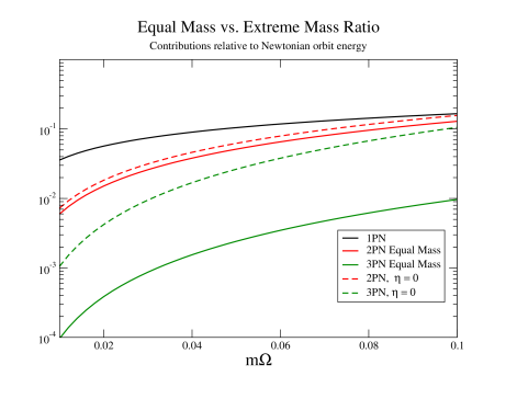
Figure 1: Contributions of 1PN, 2PN and 3PN terms to the energy, expressed as a fraction of the Newtonian energy, vs. $m\Omega$. Circular orbits are assumed. Shown are the equal mass case ($\eta=1/4$) and the point-mass limit ($\eta=0$).

First we look at the relative contributions of point-mass PN corrections. Figure 1 shows the contribution, relative to the Newtonian orbital energy, of the 1PN, 2PN and 3PN terms in the energy, for $\eta=0$ and $\eta=1/4$, as a function of $m\Omega$. Results for the angular momentum are similar. While the 1PN terms are essentially insensitive to $\eta$, and the 2PN terms are only 15 % smaller for equal masses than for the test-mass limit, the 3PN terms are suppressed for equal masses by more than a factor of 10 compared to the test-mass limit. As Blanchet luc02 ; luchopkins has argued, this suggests that the 3PN approximation may be quite accurate for comparable-mass systems, without the need for sophisticated resummation techniques. At the largest angular velocity considered, 3PN terms contribute less than one per cent of the total binding energy and angular momentum of the orbit.

Next we consider the effects of tidal and rotational distortions. We consider systems of identical bodies ($m_{1}=m_{2}$) which are corotating ($\tilde{\omega}_{1}=\tilde{\omega}_{2}=\Omega$). For neutron stars, we adopt the maximum values of the apsidal constants ($k_{2}=3/4$ and $k_{3}=3/8$, see Appendix B.3), and choose two representative values of $q=R_{a}/m_{a}$ for neutron star models with reasonable equations of state, namely $q=4$ and $q=6$. The results, plotted as a fraction of the Newtonian orbital terms, are shown in Figures 2 and 3, along with the PN contributions for comparison. As expected, tidal effects are very sensitive to the stellar radii. For $q=4$, the $l=2$ tidal terms become comparable to the 2PN and 1PN terms only around $m\Omega\sim 0.09$, while the $l=3$ terms are an order of magnitude smaller. For $q=6$, the $l=2$ tidal terms exceed the 1PN terms already by $m\Omega\sim 0.05$, while the $l=3$ terms are small, approaching the 2PN terms only at the largest allowed $m\Omega\sim 0.07$, corresponding to the point at which these larger stars are touching. For irrotational stars ($\tilde{\omega}_{1}=\tilde{\omega}_{2}=0$), the tidal effects are very similar.

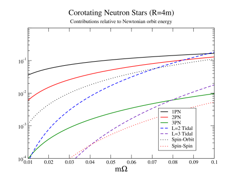
Figure 2: Contributions of tidal and spin terms to the energy for corotating neutron star binaries, expressed as a fraction of the Newtonian energy, vs. $m\Omega$, for $q=R_{a}/m_{a}=4$. Circular orbits are assumed. Shown are the PN contributions for comparison

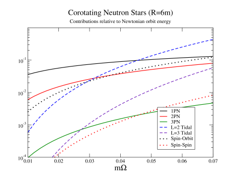
Figure 3: Same as Fig. 2, with $q=6$

These curves illustrate that tidal effects need to be taken into account carefully in an accurate diagnostic for neutron star binaries, but are not so large that they invalidate our approximation scheme. Their modest size also supports our use of Newtonian theory to calculate them. They only become problematical for the largest neutron stars near the very endpoint of their inspiral. It should also be pointed out that, in making these estimates, we have adopted the largest values of the apsidal constants, corresponding to uniform-density stars. While neutron stars are not as centrally condensed as, say, non-degenerate stars, they are also not uniform density, so the $k_{l}$ may well be smaller than their maximum values. For example, for a Newtonian polytrope, $p=k\rho^{\Gamma}$, with $\Gamma=2$, $k_{2}=0.26$, so the $q=6$ tidal terms in Fig. 3 are reduced by a factor of three, bringing them to a level at or below the 1PN terms over the whole range of $m\Omega$. On the other hand, very little, if anything, is known about the values of $k_{l}$ for general relativistic neutron stars over a range of equations of state. This is a subject that we are currently investigating.

Figure 4 shows the effects of tides for co-rotating black-hole binaries. There we choose $q=1$ ($R=m$ in harmonic coordinates), $k_{2}=3/4$ and $k_{3}=3/8$ (for slowly rotating black holes, $k_{2}$ from rotational distortions happens to be precisely $3/4$; see, eg. hartlethorne ). We see, not surprisingly, that tidal effects are utterly negligible over the entire range of $m\Omega$.

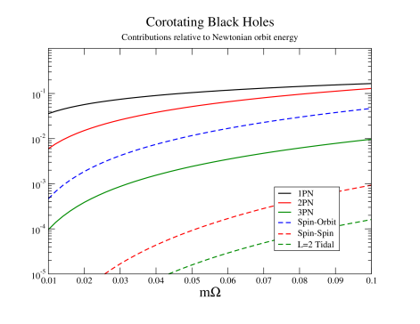
Figure 4: Same as Fig 2 but for corotating black-hole binaries, with $q=1$.

Finally, we examine spin effects. Again we consider identical, co-rotating bodies. For neutron stars, we assume that $S_{a}=I_{a}\Omega$, with the moment of inertia given by that for a uniform density body, $I_{a}=(2/5)m_{a}R_{a}^{2}=(2/5)q^{2}m_{a}^{3}$. The results are shown also in Figures 2 and 3. For $q=4$, spin-orbit effects are small but significant, just below the 2PN terms, while spin-spin effects are negligible. For $q=6$, spin-orbit terms exceed 2PN terms by $m\Omega\sim 0.04$ and become comparable to the 1PN terms by the maximum angular velocity, while spin-spin terms barely exceed the 3PN effects.

For black holes, we use the fact that $S_{a}=4m_{a}^{3}\Omega$. Figure 4 shows that the spin-orbit terms lie between the 2PN and 3PN contributions and thus must be included, while spin-spin terms are negligible (though larger than the tidal terms).

IV.2 Corotating, identical black holes

For black hole binaries, we ignore tidal and spin-spin effects. We set $m_{1}=m_{2}$, $\eta=1/4$, and $\tilde{\omega}_{1}=\tilde{\omega}_{2}=\Omega$. We exploit the fact that there exist exact formulae for the energy and spin of isolated Kerr black holes in terms of the irreducible mass, $M=M_{\rm irr}/[1-4(M_{\rm irr}\omega)^{2}]^{1/2}$, $S=4M_{\rm irr}^{3}\omega/[1-4(M_{\rm irr}\omega)^{2}]^{1/2}$. The total energy and angular momentum of the system are then given by

$$E_{\rm Tot} = E_{\rm Self}+E_{\rm Harm}+E_{\rm N,Corr}+E_{\rm Spin}\,,$$

$$J_{\rm Tot} = S+J_{\rm Harm}+J_{\rm N,Corr}+J_{\rm Spin}\,,$$ (59)

where

$$E_{\rm Self} = m_{\rm irr}\left[1+\frac{1}{2}(m_{\rm irr}\Omega)^{2}+\frac{3}{8}(m_{\rm irr}\Omega)^{4}+\dots\right]\,,$$ (60a)

$$S = m_{\rm irr}^{3}\Omega\left[1+\frac{1}{2}(m_{\rm irr}\Omega)^{2}+\frac{3}{8}(m_{\rm irr}\Omega)^{4}+\dots\right]\,,$$ (60b)

$$E_{\rm Harm} = -\frac{1}{8}m_{\rm irr}(1-e^{2})\zeta\left[1-\frac{1}{48}(37-e^{2})\zeta-\frac{1}{384}(1069-934e^{2}+129e^{4})\zeta^{2}\right.$$ (60c)

$$\left.+\left(\frac{1}{331776}(1427365+18249e^{2}-6225e^{4}-23005e^{6})-\frac{41\pi^{2}}{384}(5-e^{2})\right)\zeta^{3}\right]\,,$$

$$J_{\rm Harm} = \frac{1}{4}m_{\rm irr}^{2}\frac{1}{\sqrt{\zeta}}\left[1+\frac{1}{24}(37-e^{2})\zeta+\frac{1}{384}(1069+234e^{2}-127e^{4})\zeta^{2}\right.$$ (60d)

$$\left.-\left(\frac{1}{82944}(285473-181851e^{2}+205683e^{4}+2311e^{6})-\frac{41\pi^{2}}{96}(1+e^{2})\right)\zeta^{3}\right]\,,$$

$$E_{\rm N,Corr} = -\frac{5}{48}m_{\rm irr}(1-e^{2})(m_{\rm irr}\Omega)^{2}\zeta\,,$$ (60e)

$$J_{\rm N,Corr} = \frac{5}{24}m_{\rm irr}^{2}(m_{\rm irr}\Omega)^{2}/\sqrt{\zeta}\,,$$ (60f)

$$E_{\rm Spin} = -\frac{1}{12}m_{\rm irr}(1-e^{2})(7-2e^{2})(m_{\rm irr}\Omega)\zeta^{5/2}\,,$$ (60g)

$$J_{\rm Spin} = -\frac{5}{24}m_{\rm irr}^{2}(7+e^{2})(m_{\rm irr}\Omega)\zeta\,,$$ (60h)

where $m_{\rm irr}$ is the total irreducible mass of the system, given by $(m_{\rm irr})_{1}+(m_{\rm irr})_{2}$. In Eqs. (60a) and (60b), we have expanded the Kerr formulae for $M$ and $S$ in powers of $m_{\rm irr}\Omega$, assumed to be small compared to unity, keeping as many higher-order terms as needed to reach a precision comparable to our 3PN formulae. To obtain $E_{\rm Tot}$ and $J_{\rm Tot}$ at a turning point as functions of $\Omega$, we substitute $\zeta=(m_{\rm irr}\Omega_{a})^{2/3}/(1-e)^{4/3}$ or $\zeta=(m_{\rm irr}\Omega_{p})^{2/3}/(1+e)^{4/3}$ for apocenter or pericenter, respectively (in calculating $E_{\rm N,Corr}$ and $J_{\rm N,Corr}$, we have already changed the dependence in $\zeta$ from the total mass of the rotating bodies to the total irreducible mass of the non-rotating counterparts). These are the formulas used in morawill to compare with the numerical HKV quasi-equilibrium solutions of Grandclément et al. ggb02 . When $E_{\rm Tot}$ and $J_{\rm Tot}$ are scaled by $m_{\rm irr}$ and $m_{\rm irr}^{2}$ respectively, there remains only one free parameter, the eccentricity of the orbit, and we found morawill that a substantially better fit to the numerical data was obtained for non-zero values of $e$, of the order of $0.03$, with the system at apocenter, than for $e=0$. We suggested that such apparent eccentricity could be a result of the inevitable approximations (such as the conformally flat approximation) and numerical errors in such initial-data models, but, in the absence of detailed estimates of the sizes of those errors, it was difficult to draw firm conclusions. On the other hand, those engaged in numerical models of black hole binaries could use our diagnostic as a guide to know when, say, a suitable circular orbit has been achieved, or whether further numerical experiments with different grid sizes or larger computational domains are necessary to reach the desired physically meaningful state.

IV.3 Corotating, identical neutron stars

For neutron stars, we must include tidal effects. We set $m_{1}=m_{2}$, $\eta=1/4$, and $\tilde{\omega}_{1}=\tilde{\omega}_{2}=\Omega$; we let the apsidal constants and radius factors be common for both stars, given by $k_{2}$, $k_{3}$, and $q$, respectively, and express all quantities in terms of the total mass $m_{0}=(m_{0})_{1}+(m_{0})_{2}$ of two non-rotating stars with the same equation of state. We also define for each star the coefficient $\alpha_{a}=I_{a}/m_{a}R_{a}^{2}$, and also assume it to be common for both stars. The result is

$$E_{\rm Tot} = E_{\rm Self}+E_{\rm Harm}+E_{\rm N,Corr}+E_{\rm Spin}+E_{\rm TR,Orbit}+E_{\rm Distort}\,,$$

$$J_{\rm Tot} = S+J_{\rm Harm}+J_{\rm N,Corr}+J_{\rm Spin}+J_{\rm TR,Orbit}+J_{\rm Distort}\,,$$ (61)

where the 3PN point-mass expressions $E_{\rm Harm}$ and $J_{\rm Harm}$ are given in Eqs. (60c) and (60d), and where

$$E_{\rm Self} = m_{0}+\frac{1}{8}\alpha q^{2}m_{0}(m_{0}\Omega)^{2}\,,$$ (62a)

$$S = \frac{1}{4}\alpha q^{2}m_{0}^{2}(m_{0}\Omega)\,,$$ (62b)

$$E_{\rm N,Corr} = -\frac{5}{192}m_{0}(1-e^{2})\alpha q^{2}(m_{0}\Omega)^{2}\zeta\,,$$ (62c)

$$J_{\rm N,Corr} = \frac{5}{96}m_{0}^{2}\alpha q^{2}(m_{0}\Omega)^{2}/\sqrt{\zeta}\,,$$ (62d)

$$E_{\rm Spin} = -\frac{1}{48}m_{0}(1-e^{2})(7-2e^{2})\alpha q^{2}(m_{0}\Omega)\zeta^{5/2}\,,$$ (62e)

$$J_{\rm Spin} = -\frac{5}{96}m_{0}^{2}(7+e^{2})\alpha q^{2}(m_{0}\Omega)\zeta\,,$$ (62f)

$$E_{\rm TR,Orbit} = \frac{1}{32}m_{0}(1-e^{2})\left[\frac{1}{9}(3-e^{2})q^{5}k_{2}(m_{0}\Omega)^{2}\zeta^{3}+\frac{1}{6}(9+10e^{2}-3e^{4})q^{5}k_{2}\zeta^{6}\right.$$ (62g)

$$\left.+\frac{1}{24}(13+49e^{2}+7e^{4}-5e^{6})q^{7}k_{3}\zeta^{8}\right]\,,$$

$$J_{\rm TR,Orbit} = \frac{1}{32}m_{0}^{2}\left[\frac{2}{9}(3+e^{2})q^{5}k_{2}(m_{0}\Omega)^{2}\zeta^{3/2}+\frac{2}{3}(3+10e^{2}+3e^{4})q^{5}k_{2}\zeta^{9/2}\right.$$ (62h)

$$\left.+\frac{2}{3}(1+7e^{2}+7e^{4}+e^{6})q^{7}k_{3}\zeta^{13/2}\right]\,,$$

$$E_{\rm Distort} = \frac{1}{48}m_{0}q^{5}k_{2}(m_{0}\Omega)^{2}[(m_{0}\Omega)^{2}+(1-\epsilon e)^{3}\zeta^{3}]\,,$$ (62i)

$$J_{\rm Distort} = \frac{1}{144}m_{0}^{2}q^{5}k_{2}(m_{0}\Omega)[4(m_{0}\Omega)^{2}+3(1-\epsilon e)^{3}\zeta^{3}]\,.$$ (62j)

We illustrate the use of this diagnostic by comparing with numerical data recently reported by Miller et al. mgs03 . They constructed a sequence of general relativistic, quasi-equilibrium configurations of corotating neutron stars, in the conformally flat approximation. They used a polytropic equation of state with $\Gamma=2$. Among other quantities, they report an “effective” binding energy, given by $E_{b}=[M_{\rm ADM}-2M_{\rm NS}(\Omega)]/M_{0}$, as a function of $M_{0}\Omega$, where $M_{\rm ADM}$ is the total ADM mass of the configuration, and $M_{\rm NS}(\Omega)$ is the ADM mass of a uniformly rotating isolated neutron star of the same baryonic mass $M_{0}$, as each star in the binary configuration, but rotating with angular velocity $\Omega$. Since the rotational kinetic energy of the stars is already removed, we can compare the numerical results with the PN diagnostic $E_{\rm Diag}=[E_{\rm Tot}-E_{\rm Self}]/m_{0}$. Since our $m_{0}$ is twice the ADM mass of a non-rotating neutron star, we must scale $E_{b}$ by $M_{0}/2M_{\rm ADM-NS}$, where $M_{\rm ADM-NS}$ is the ADM mass of an isolated, non-rotating neutron star. In the models of Miller et al., $M_{\rm ADM-NS}=M_{0}/1.067$. We also need to fix the coefficients $q$ and $\alpha$. From data provided by Miller (private communication), the radius of each isolated non-rotating star in isotropic coordinates is given by $R_{I}=6.77M_{\rm ADM}$,while the baryonic moment of inertia, calculated using isotropic coordinates, is given by $I_{0}=9.412M_{0}^{3}$. We work in harmonic coordinates, but since $R_{H}=R_{I}(1+M_{\rm ADM}^{2}/4R_{I}^{2})$, the difference between the two coordinates is only of order 1/2 %, so we read off $q=6.77$. The ADM moment of inertia can be identified as $I_{\rm ADM}=(M_{\rm ADM}/M_{0})I_{0}=9.412M_{\rm ADM}M_{0}^{2}=9.412(1.067)^{2}M_{\rm ADM}^{3}$. Thus we can read off $\alpha q^{2}=9.412(1.067)^{2}$ and hence $\alpha=0.234$, or around half of the uniform-density value of 2/5. (Miller also calculates the same quantities in terms of circumferential, or Schwarzschild radius; after transforming to harmonic coordinates, the results for $q$ and $\alpha$ are consistent with these to within a few per cent.)

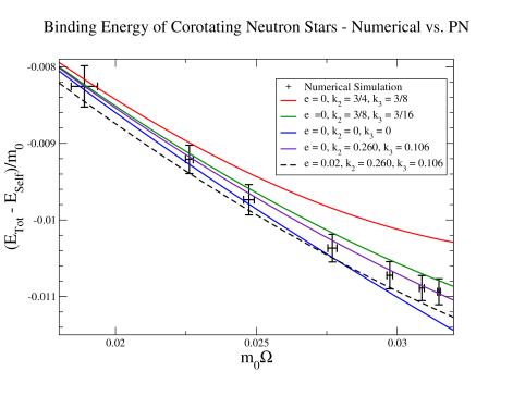
Figure 5: Comparison of PN diagnostic with numerical initial-data models of mgs03 .

Inserting these values of $q$ and $\alpha$ into our diagnostic, we compare various PN configurations with those reported by Miller et al., as shown in Figure 5. The numerical results are shown as “$+$” with error bars, estimated by Miller et al. from the results of a range of convergence tests. Four curves show the energy for circular orbits, for various values of the apsidal constants. Neither the uniform-density values ($k_{2}=3/4$, $k_{3}=3/8$), nor the point mass values ($k_{2}=0$, $k_{3}=0$) gives a good fit at all, except at low angular velocities (large separations) where tidal effects are smaller, and all circular-orbit curves converge toward the numerical result. Models with half the uniform-density values for $k_{2}$ and $k_{3}$ give marginal fits. However, a very good fit is achieved with values $k_{2}=0.260$ and $k_{3}=0.106$; these are precisely the values for Newtonian $\Gamma=2$ polytropes (Appendix B), which is the equation of state used in the Miller et al. numerical models. Also shown is a model with the same $\Gamma=2$ apsidal constants, but with a non-zero eccentricity $e=0.02$ and with the system at apocenter. This marginally fits the numerical data within the error bars, but consistently gives lower (more negative) energies.

We conclude that these quasi-equilibrium neutron-star configurations are fit to better than one per cent by our PN diagnostic with a circular orbit, and with physically reasonable tidal terms.

In future work we plan to compare this diagnostic with results of other numerical models of quasi-equilibrium black hole and neutron star binaries. Our 3PN equations of motion, together with tidal and spin terms, augmented by radiation reaction terms, can also be used to develop a “dynamical” diagnostic, to compare with numerical simulations of evolutions from the quasi-equilibrium initial data mgs03 ; mdsb03 .

Appendix A Newtonian Tidal and Rotational Effects

A.1 Distorted equilibrium configurations

To derive the effects of tidal and rotational flattening, we will adopt standard methods from Newtonian theory for binary systems, such as those detailed by Kopal kopal1 ; kopal2 . We assume that the timescale for changes in perturbing quantities (such as the external tidal potential, seen either from the global inertial frame, or from the rotating frame of a given body) is sufficiently long that each body can be assumed to be in hydrostatic equilibrium. In other words, we will ignore dynamical tides dynamicaltides . This is a reasonable assumption as long as we are focusing on quasi-equilibrium initial data. Consider one of the bodies in the binary system. From the equation of hydrostatic equilibrium, $\nabla p=\rho\nabla\Psi$, where $p$, $\rho$ and $\Psi$ are the pressure, density and total gravitational potential, respectively, we conclude that $\nabla\rho\times\nabla\Psi=0$, and thus that surfaces of constant $\rho$ and $\Psi$ coincide. We label surfaces of constant $\rho$ by the radial parameter $a$, and let the equation of those surfaces have the form

$$r(a,\theta,\phi)=a[1+\sum_{l,m}f_{lm}(a)Y_{lm}(\hat{\Omega})]\,,$$ (63)

where $Y_{lm}(\hat{\Omega})$ are spherical harmonics corresponding to the direction ${\hat{\Omega}}$, and where the dimensionless distortion functions $f_{lm}$ have the property $f_{lm}^{*}=(-1)^{m}f_{l,-m}$.

On general grounds we expect $f_{lm}\sim(R/r)^{l+1}\sim q^{l+1}(m/r)^{l+1}$ for tidal effects, and, for $l=2$, $f_{2m}\sim\omega^{2}/\rho\sim(R/r)^{3}\sim q^{3}(m/r)^{3}$ from rotational effects. The effect of these distortions on the external potential of a body is of order $f_{lm}(R/r)^{l}\sim q^{2l+1}(m/r)^{2l+1}$. For $l=2$, this means effectively 5PN order; $l=3$ effects would be effectively 7PN order, and so on. However, for neutron stars, with $q\sim 4$ and $m/r\sim 0.1$, an $l=2$ distortion effect becomes numerically comparable to a 2PN term, while $l=3$ is comparable to a 3PN term. For black holes, with $q<1$, the effects are much smaller. Thus, in the end, we will keep only $l=2$ and $l=3$ distortion terms. Also, non linear corrections to $f_{lm}$ would be of order $(R/r)^{l+1}\sim q^{l+1}(m/r)^{l+1}$ smaller than the dominant linear effects, and thus, effectively of 8PN order for $l=2$ (for neutron stars, these non-linear corrections would be numerically smaller than 3PN). The exception to this is in the internal gravitational energy of each body, where a quadratic contribution yields $(m^{2}/R){f_{lm}}^{2}\sim(m^{2}/r)(R/r)^{2l+1}$, which is comparable to the other effectively 5PN contributions for $l=2$.

We begin, however, with a general analysis, keeping $lm$ arbitrary, and working to second order in the small quantities $f_{lm}$. Later (Appendix B) we will specialize to $l=2$ and $l=3$ linear perturbations. To second order, it is straightforward to show that, for any $n$,

$$r^{n}=a^{n}\{1+n\sum_{l,m}[f_{lm}(a)+(n-1)X_{lm}]Y_{lm}(\hat{\Omega})\}\,,$$ (64)

where

$$X_{lm}\equiv\frac{1}{2}\sum_{\alpha\beta;\gamma\delta}C^{lm}_{\alpha\beta;\gamma\delta}f_{\alpha\beta}f_{\gamma\delta}\,,$$ (65)

and $C^{lm}_{\alpha\beta;\gamma\delta}$ is defined in terms of Clebsch-Gordan coefficients,

$$C^{lm}_{\alpha\beta;\gamma\delta}=\sqrt{\frac{(2\alpha+1)(2\gamma+1)}{4\pi(2l+1)}}\left(\begin{array}[]{ccc}\alpha&\gamma&l\\ 0&0&0\end{array}\right)\left(\begin{array}[]{ccc}\alpha&\gamma&l\\ \beta&\delta&m\end{array}\right)\,.$$ (66)

Note that the various angular momentum quantum numbers are connected by the constraints $l=\alpha+\gamma\,,\alpha+\gamma-2\,,\dots\,,|\alpha-\gamma|$, and $m=\beta+\delta$; the $C^{lm}_{\alpha\beta;\gamma\delta}$ are symmetric under $(\alpha\beta)\rightleftharpoons(\gamma\delta)$. Also note that $X_{00}=(16\pi)^{-1/2}\sum_{\alpha\beta}f_{\alpha\beta}f_{\alpha\beta}^{*}$.

We expand the gravitational potential $U$ of the body and the disturbing potential $V$ in the form

$$U = \sum_{lm}\frac{4\pi}{2l+1}\int\rho({\bf x}^{\prime})\frac{r_{<}^{l}}{r_{>}^{l+1}}Y^{*}_{lm}({\hat{\Omega}}_{<})Y_{lm}({\hat{\Omega}}_{>})d^{3}x^{\prime}\,,$$

$$V = \tilde{d}r^{2}+\sum_{lm}\frac{4\pi}{2l+1}d_{lm}r^{l}Y_{lm}({\hat{\Omega}})\,,$$ (67)

where the subscript $>(<)$ corresponds to the larger (smaller) of $r$ and $r^{\prime}$. The disturbing potential consists of a part, with disturbing coefficients $d_{lm}$, that corresponds to a potential with $\nabla^{2}V=0$, such as the gravitational potential from another body, or the Laplacian-free part of a centrifugal potential, plus the spherical part of a centrifugal potential, with coefficient $\tilde{d}$. We now substitute Eqs. (63) and (64) into (67), convert all expressions from $r$ to $a$, and demand that, for $l=0$, the external gravitational potential of our body have the form $U=m/r$ (i.e. the perturbation does not change the mass of the body), and that, for $l\neq 0$, the total potential $U+V$ be constant at a given $a$. The first can be satisfied if $f_{00}+2X_{00}=0$, while the second holds if, for $l\neq 0$,

$$a^{-l-1}F_{lm}(a) + a^{l}E_{lm}(a)-\frac{2l+1}{4\pi}\frac{m(a)}{a}f_{lm}(a)+a^{l}d_{lm}$$ (68)

$$= {\sum_{\alpha\beta;\gamma\delta}}^{\prime}\frac{2l+1}{2\alpha+1}C^{lm}_{\alpha\beta;\gamma\delta}f_{\gamma\delta}\biggl{[}(\alpha+1)a^{-\alpha-1}F_{\alpha\beta}(a)-\alpha a^{\alpha}(E_{\alpha\beta}(a)+d_{\alpha\beta})\biggr{]}$$

$$-\frac{2l+1}{2\pi}\frac{m(a)}{a}X_{lm}(a)-2(2l+1)\tilde{d}a^{2}f_{lm}\,,$$

where

$$m(a) = \int_{0}^{a}4\pi\rho(a)a^{2}da\,,$$

$$F_{lm}(a) = \int_{0}^{a}\rho(a)da\frac{d}{da}\biggl{[}a^{l+3}(f_{lm}+(l+2)X_{lm})\biggr{]}\,,$$

$$E_{lm}(a) = \int_{a}^{A}\rho(a)da\frac{d}{da}\biggl{[}a^{2-l}(f_{lm}+(1-l)X_{lm})\biggr{]}\,,$$ (69)

and $A$ denotes the surface of the body. The left-hand-side of Eq. (68) is first order in $f_{lm}$, while the right-hand-side is second-order. Dividing the first-order terms by $a^{l}$, differentiating with respect to $a$ and multiplying by $a^{2l+2}$, we obtain the first-order result

$$F_{lm}(a)=\frac{m(a)a^{l}}{4\pi}[(l+1)f_{lm}-af_{lm}^{\prime}]\,,$$ (70)

where prime denotes differentiation with respect to $a$. Substituting this and the first-order solution of Eq. (68) back into the right-hand-side of Eq. (68), it is straightforward to show that the term involving ${\sum^{\prime}_{\alpha\beta;\gamma\delta}}$ reduces to $m(a)(2X_{lm}-aX_{lm}^{\prime})/4\pi a$, to second order. The basic equation for the distortion functions $f_{lm}$ can then be written in the form of an integral equation

$$\frac{2l+1}{4\pi}m(a)f_{lm}(a) - a^{-l}\int_{0}^{a}\rho(a^{l+3}f_{lm})^{\prime}da-a^{l+1}\int_{a}^{A}\rho(a^{2-l}f_{lm})^{\prime}da$$ (71)

$$= a^{l+1}d_{lm}+{\cal R}_{lm}(a)\,,$$

where ${\cal R}_{lm}$ contains all contributions quadratic in small quantities:

$${\cal R}_{lm}(a) = \frac{2l+1}{4\pi}am(a)X_{lm}^{\prime}+2(2l+1)\tilde{d}a^{2}f_{lm}$$ (72)

$$+(l+2)a^{-l}\int_{0}^{a}\rho(a^{l+3}X_{lm})^{\prime}da$$

$$-(l-1)a^{l+1}\int_{a}^{A}\rho(a^{2-l}X_{lm})^{\prime}da\,.$$

Combining Eq. (71) with various derivatives of it, one obtains the following useful equations, evaluated at the surface $a=A$ of the star:

$$(l+1)f_{lm}(A)-Af_{lm}^{\prime}(A)+{\cal P}_{lm} = \frac{4\pi}{m}A^{-l}\int_{0}^{A}\rho[a^{l+3}(f_{lm}+(l+2)X_{lm})]^{\prime}da\,,$$ (73a)

$$lf_{lm}(A)+Af_{lm}^{\prime}(A)-{\cal Q}_{lm} = \frac{4\pi}{m}A^{l+1}d_{lm}\,,$$ (73b)

where $m=\int_{0}^{A}4\pi\rho a^{2}da$, and

$${\cal P}_{lm} = A^{2}X_{lm}^{\prime\prime}(A)-lAX_{lm}^{\prime}(A)+\frac{8\pi}{m}\tilde{d}A^{2}[Af_{lm}^{\prime}(A)-(l-1)f_{lm}(A)]\,,$$

$${\cal Q}_{lm} = A^{2}X_{lm}^{\prime\prime}(A)+(l+1)AX_{lm}^{\prime}(A)]+\frac{8\pi}{m}\tilde{d}A^{2}[Af_{lm}^{\prime}(A)+(l+2)f_{lm}(A)]\,.$$ (74)

Another combination of first and second derivatives of Eq. (71) yields a second-order differential equation for $f_{lm}$, sometimes called Clairaut’s equation:

$$a^{2}f_{lm}^{\prime\prime}+\frac{8\pi\rho a^{3}}{m(a)}(af_{lm}^{\prime}+f_{lm})-l(l+1)f_{lm}=\frac{4\pi}{m(a)}[a^{2}{\cal R}_{lm}^{\prime\prime}-l(l+1){\cal R}_{lm}]\,.$$ (75)

For a given density distribution $\rho(a)$, this equation can be solved, subject to the boundary conditions that $f_{lm}$ be regular at $a=0$, and that, at the surface, $f_{lm}$ satisfy Eq. (73b).

A.2 Energy and angular momentum of the system

Given a solution for the distortion functions $f_{lm}(a)$, we can calculate all the quantities needed for the equations of motion and the energy and angular momentum of the orbit. The external potential of our body, for example, is given by

$$U = \frac{m}{r}+{\sum_{lm}}^{\prime}\frac{4\pi}{2l+1}\frac{Y_{lm}({\hat{\Omega}})}{r^{l+1}}\int_{0}^{A}\rho[a^{l+3}(f_{lm}+(l+2)X_{lm})]^{\prime}da$$ (76)

$$= \frac{m}{r}+{\sum_{lm}}^{\prime}\frac{4\pi}{2l+1}\frac{Y_{lm}({\hat{\Omega}})}{r^{l+1}}\frac{mA^{l}}{4\pi}[(l+1)f_{lm}(A)-Af_{lm}^{\prime}(A)+{\cal P}_{lm}]$$

$$= \frac{m}{r}+{\sum_{lm}}^{\prime}\frac{8\pi}{2l+1}\frac{A^{2l+1}}{r^{l+1}}k_{lm}d_{lm}Y_{lm}({\hat{\Omega}})\,,$$

where $\sum^{\prime}$ denotes summation for $l\neq 0$, and where we define the “apsidal constant” $k_{lm}$ by

$$k_{lm}\equiv\frac{1}{2}\frac{(l+1)f_{lm}(A)-Af_{lm}^{\prime}(A)+{\cal P}_{lm}}{lf_{lm}(A)+Af_{lm}^{\prime}(A)-{\cal Q}_{lm}}\,.$$ (77)

The total gravitational energy of the system is given by

$$W=-\frac{1}{2}\int\int\frac{\rho({\bf x})\rho({\bf x}^{\prime})}{|{\bf x}-{\bf x}^{\prime}|}d^{3}xd^{3}x^{\prime}=W_{11}+W_{12}+(1\rightleftharpoons 2)\,.$$ (78)

The self-energy $W_{11}$ of body 1 can be written

$$W_{11}=-\sum_{lm}\frac{4\pi}{2l+1}\int_{0}^{R}\rho r^{1-l}drd\Omega Y_{lm}({\hat{\Omega}})\int_{0}^{r}\rho^{\prime}{r^{\prime}}^{l+2}dr^{\prime}d\Omega^{\prime}Y_{lm}^{*}({\hat{\Omega}}^{\prime})\,.$$ (79)

Substituting Eqs. (63) and (64) we find no contribution linear in $f_{lm}$. To second order, we obtain

$$W_{11} = -\int_{0}^{A}\frac{m(a)}{a}dm(a)$$ (80)

$$+{\sum_{lm}}^{\prime}\frac{1}{2l+1}\int_{0}^{A}\rho(a)m(a)ada\biggl{[}a^{2}|{f_{lm}^{\prime}}|^{2}+2af_{lm}^{*}{f_{lm}^{\prime}}+(l^{2}+l-1)|{f_{lm}}|^{2}\biggr{]}\,.$$

Since the second term is already second order, we can integrate by parts and use the first-order versions of Eqs. (73) and (75) to obtain the alternative form

$$W_{11}=-{\cal W}+{\sum_{lm}}^{\prime}\frac{4\pi}{2l+1}A^{2l+1}|{d_{lm}}|^{2}k_{lm}\,,$$ (81)

where we define the self-gravitational binding energy $\cal W$ of the undistorted configuration by

$${\cal W}=\int_{0}^{A}\frac{m(a)}{a}dm(a)\,.$$ (82)

In $W_{12}$, we substitute the external potential of body 2 evaluated inside body 1, to obtain

$$W_{12}=-\frac{1}{2}\int_{1}\rho d^{3}x\left(\frac{m_{2}}{y_{2}}+{\sum_{lm}}^{\prime}\frac{8\pi}{2l+1}\frac{A_{2}^{2l+1}}{y_{2}^{l+1}}d_{lm}^{(2)}k_{lm}^{(2)}Y_{lm}({\hat{y}}_{2})\right)\,,$$ (83)

where ${\bf y}_{2}={\bf x}-{\bf x}_{2}$, $k_{lm}^{(2)}$ is the apsidal constant of body 2, and $d_{lm}^{(2)}$ is the coefficient of the disturbing potential acting on body 2. Since the interaction energy is smaller than the self energy by a factor of $R/r$, we only need to keep terms linear in the deformations $f_{lm}$ or the disturbing coefficients $d_{lm}$; consequently we carry out a multipole expansion of $1/y_{2}$ in the first term in Eq. (83), then convert from $r$ to $a$ using Eq. (63), but we evaluate the second term at the center of mass of body 1 and do the lowest-order spherical integral. Effectively, we are ignoring multipole-multipole coupling between the bodies, which can be shown to lead to effects of order $(A/r)^{2l+1}(A/r)^{2n+1}\sim(m/r)^{10}$, or 10PN order for $l=n=2$. The result is

$$W_{12}=-\frac{1}{2}\frac{m_{1}m_{2}}{r}-\sum_{lm}\frac{4\pi}{2l+1}\left(m_{1}A_{2}^{2l+1}d_{lm}^{(2)}k_{lm}^{(2)}+(-1)^{l}m_{2}A_{1}^{2l+1}d_{lm}^{(1)}k_{lm}^{(1)}\right)\frac{Y_{lm}({n})}{r^{l+1}}\,,$$ (84)

where now $r=|{\bf x}_{1}-{\bf x}_{2}|$ and ${\bf n}=({\bf x}_{1}-{\bf x}_{2})/r$. Combining Eqs. (81) and (84), the final result is

$$W = -{\cal W}_{1}-\frac{1}{2}\frac{m_{1}m_{2}}{r}$$ (85)

$$+\sum_{lm}\frac{4\pi}{2l+1}A_{1}^{2l+1}d_{lm}^{(1)}k_{lm}^{(1)}\left(d_{lm}^{*(1)}-2(-1)^{l}\frac{m_{2}}{r^{l+1}}Y_{lm}({n})\right)$$

$$+(1\rightleftharpoons 2)\,,$$

where, under the interchange, ${\bf n}\to-{\bf n}$.

The kinetic energy of the system is given by $T=\int\rho v^{2}d^{3}x$. Splitting the velocity of an element of fluid into center-of-mass, rotational, and random parts, and noting that

$$\sum_{m}Y_{lm}^{*}({n})Y_{lm}({n}^{\prime})=\frac{(2l+1)!!}{4\pi l!}{n}^{<L>}{n^{\prime}}^{<L>}=\frac{2l+1}{4\pi}P_{l}({\bf n}\cdot{\bf n}^{\prime})\,,$$ (86)

where ${\hat{n}}^{<L>}$ denotes an STF product of $l$ unit vectors (a capitalized superscript denotes a multi-index), the product ${n}^{<L>}{n^{\prime}}^{<L>}$ denotes contraction on all indices, and $P_{l}$ is a Legendre polynomial, we may write

$$T=\frac{1}{2}m_{1}v_{1}^{2}+T_{\rm Thermal}^{(1)}+\frac{1}{3}\omega_{1}^{2}\int_{0}^{R_{1}}\rho r^{2}drd\Omega\left(1-\frac{4\pi}{5}\sum_{m}Y_{2m}({\hat{\lambda}}_{1})Y_{2m}^{*}({\hat{\Omega}})\right)+(1\rightleftharpoons 2)\,,$$ (87)

where $\mbox{\boldmath$\mathsf{\hat{\lambda}}$}_{1}=\mbox{\boldmath$\mathsf{\omega}$}_{1}/\omega_{1}$. Converting from $r$ to $a$ using Eq. (63), recalling that $f_{00}=-2X_{00}$, and noting that $\omega^{2}$ is already of first order in disturbing quantities, we obtain, to second order in small quantities,

$$T=\frac{1}{2}m_{1}v_{1}^{2}+T_{\rm Thermal}^{(1)}+\frac{1}{2}I_{1}\omega_{1}^{2}-\frac{8\pi}{15}\omega_{1}^{2}A_{1}^{5}\sum_{m}d_{2m}^{(1)}k_{2m}^{(1)}Y_{2m}({\hat{\lambda}}_{1})+(1\rightleftharpoons 2)\,,$$ (88)

where $I_{1}=(2/3)\int_{0}^{A_{1}}4\pi\rho a^{4}da$.

The angular momentum of the system is given by $J^{i}=\epsilon^{ijk}\int\rho x^{j}v^{k}$. Using the same split of the velocities, we obtain, to the analogous order of precision,

$$J^{i}=m_{1}({\bf x}_{1}\times{\bf v}_{1})^{i}+I_{1}\omega_{1}^{i}-2\omega_{1}^{j}A_{1}^{5}\sum_{m}d_{2m}^{(1)}k_{2m}^{(1)}Z_{2m}^{<ij>}+(1\rightleftharpoons 2)\,,$$ (89)

where we define the symmetric trace free (STF) tensor

$$Z_{lm}^{<L>}\equiv\int Y_{lm}({\hat{\Omega}}){\hat{n}}^{<L>}d^{2}\Omega\,,$$ (90)

with the following properties

$$\sum_{m}Y_{lm}^{*}({\hat{\lambda}})Z_{lm}^{<L>} = {\hat{\lambda}}^{<L>}\,,$$

$${\hat{\lambda}}^{L}Z_{lm}^{<L>} = \frac{4\pi l!}{(2l+1)!!}Y_{lm}({\hat{\lambda}})\,.$$ (91)

A.3 Equations of motion

The Newtonian equations of motion for body 1 are given by

$$a_{1}^{i}=\frac{1}{m_{1}}\int_{1}\rho d^{3}x\int_{2}\rho^{\prime}\nabla^{i}\frac{1}{|{\bf x}-{\bf x}^{\prime}|}d^{3}x^{\prime}\,.$$ (92)

We write ${\bf x}={\bf x}_{1}+\bar{\bf x}$ and ${\bf x}^{\prime}={\bf x}_{2}+\bar{\bf x}^{\prime}$ and expand in a Taylor series about ${\bf x}_{1}$ and ${\bf x}_{2}$. We define the STF multipole moments $I_{a}^{<Q>}=\int_{a}\rho\bar{x}^{<Q>}d^{3}x$ with $I_{a}^{0}=m_{a}$ and $I_{a}^{j}=0$. Finally, we calculate the relative acceleration $a^{i}=a_{1}^{i}-a_{2}^{i}$. After some manipulation, we obtain the general result

$$a^{i} = -\frac{mx^{i}}{r^{3}}+m\sum_{l=2}^{\infty}\frac{1}{l!}\left(\frac{I_{1}^{<L>}}{m_{1}}+(-1)^{l}\frac{I_{2}^{<L>}}{m_{2}}\right)\nabla^{iL}\left(\frac{1}{r}\right)$$ (93)

$$+m\sum_{l=4}^{\infty}\sum_{p=2}^{l-2}\frac{(-1)^{l-p}}{p!(l-p)!}\left(\frac{I_{1}^{<P}}{m_{1}}\frac{I_{2}^{L-P>}}{m_{2}}\right)\nabla^{iL}\left(\frac{1}{r}\right)\,,$$

where $m=m_{1}+m_{2}$ and the products of the multipole moment tensors are to be symmetrized on all indices and made trace-free. For our distorted bodies, the STF multipole moments can be shown to be given by

$$I_{1}^{<L>}=2A_{1}^{2l+1}\sum_{m}d_{lm}^{(1)}k_{lm}^{(1)}Z_{lm}^{<L>}\,.$$ (94)

With the coefficients $d_{lm}\sim m/r^{l+1}$, we have that $I^{<L>}\sim mA^{2l+1}/r^{l+1}$, and therefore the multipole-multipole coupling term in the equation of motion (93) is of order $(m/r^{2})(A/r)^{2q+2}$; since $q\geq 4$, this is 10PN and higher. As before, we ignore multipole-multipole terms.

A.4 Multiple disturbance sources

We will want to consider both tidal disturbances as well as rotation-induced disturbances. To see how this affects our general results, we note that the non-linear corrections to the Clairaut equations never play a role to the order of accuracy we require, only the linear functions $f_{lm}$, satisfying linear differential equations, are needed in the end. Let $f_{lm}=g_{lm}+h_{lm}$, where each disturbance function satisfies the linearized Clairaut equations (75), with a boundary condition for each determined by the linearized Eq. (73b). From the structure of the formulae for the external potential $U$, the kinetic energy, the angular momentum, and the multipole moments, it is clear that the coefficient $d_{lm}k_{lm}$ can simply be replaced by $d_{lm}^{(g)}k_{lm}^{(g)}+d_{lm}^{(h)}k_{lm}^{(h)}$, where $d_{lm}^{(\alpha)}$ is the amplitude of the disturbing function for that disturbance, and $k_{lm}^{(\alpha)}$ is the corresponding apsidal constant, determined from the linearized Eq. (77). However because it has a contribution quadratic in disturbing functions, the gravitational self-energy $W_{11}$ requires some care. Returning to the expression (80), substituting $f_{lm}=g_{lm}+h_{lm}$ and carrying out the integrations by parts, using the linearized Clairaut equations satisfied separately by $g_{lm}$ and $h_{lm}$, one can show that the coefficient $|{d_{lm}}|^{2}k_{lm}$ must be replaced by the coefficient $|{d_{lm}^{(g)}}|^{2}k_{lm}^{(g)}+|{d_{lm}^{(h)}}|^{2}k_{lm}^{(h)}+k_{lm}^{(g)}d_{lm}^{(g)}d_{lm}^{*(h)}+k_{lm}^{(h)}d_{lm}^{(h)}d_{lm}^{*(g)}$.

Appendix B Rotational and $l=2$, $l=3$ tidal distortions

B.1 Disturbing coefficients and apsidal constants

We focus on the lowest-order $l=2$ and $l=3$ tidal terms. The gravitational potential at a point ${\bf x}^{\prime}$ in body 1 due to body 2 is given by

$$V=m_{2}\sum_{lm}\frac{4\pi}{2l+1}\frac{{r^{\prime}}^{l}}{r^{l+1}}(-1)^{l}Y_{lm}^{*}(n)Y_{lm}({\hat{\Omega}}^{\prime})\,,$$ (95)

where we ignore the contributions to $V$ from the distortions of body 2 (ignore multipole-multipole coupling). We thus obtain the tidal coefficient for body 1,

$$d_{lm}^{T(1)}=m_{2}(-1)^{l}Y_{lm}^{*}({n})/r^{l+1}\,,$$ (96)

with the coefficient for body 2 obtained by interchange. Working to linearized order, we can factor out the azimuthal $m$ dependence by defining $f_{lm}^{T}=f_{l}^{T}Y_{lm}^{*}({\hat{n}})$, then the Clairaut equation and the outer boundary condition for body 1 take the form

$$a^{2}{f_{l}^{T}}^{\prime\prime}+\frac{8\pi\rho a^{3}}{m(a)}(a{f_{l}^{T}}^{\prime}+f_{l}^{T})-l(l+1)f_{l}^{T} = 0\,,$$ (97a)

$$A_{1}{f_{l}^{T}}^{\prime}(A_{1})+lf_{l}^{T}(A_{1}) = 4\pi(-1)^{l}\frac{m_{2}}{m_{1}}\left(\frac{A_{1}}{r}\right)^{l+1}\,.$$ (97b)

Note that the apsidal constant depends only on $f_{l}^{T}$, and is thus independent of $m$, so

$$k_{l}^{T(1)}=\frac{l+1-\eta_{l}^{T}(A_{1})}{2l+2\eta_{l}^{T}(A_{1})}\,,$$ (98)

with a corresponding expression for body 2, where

$$\eta_{l}^{T}\equiv\frac{d(\ln f_{l}^{T})}{d(\ln a)}\,.$$ (99)

Note that the overall scale of $f_{l}^{T}$ has no effect on the apsidal constant, to linear order.

For a uniformly rotating body, the disturbing potential at a point ${\bf x}^{\prime}$ is the centrifugal potential

$$V_{\rm Rot} = \frac{1}{2}\omega^{2}[{r^{\prime}}^{2}-(\mbox{\boldmath$\mathsf{\hat{\lambda}}$}\cdot{\bf x}^{\prime})^{2}]$$ (100)

$$= \frac{1}{3}\omega^{2}{r^{\prime}}^{2}-\frac{4\pi}{15}\omega^{2}{r^{\prime}}^{2}\sum_{m}Y_{2m}^{*}({\hat{\lambda}})Y_{2m}({\hat{\Omega}}^{\prime})\,.$$

Thus we read off the rotational coefficient for body 1

$${d_{2m}^{R}}^{(1)}=-\frac{1}{3}\omega_{1}^{2}Y_{2m}^{*}({\hat{\lambda}}_{1})$$ (101)

with the coefficient for body 2 obtained by interchange (the spherical coefficient $\tilde{d}$ only contributes at second order in small quantities). Similarly defining $f_{2m}^{R}=f_{2}^{R}Y_{2m}^{*}({\hat{\lambda}})$, we find that $f_{2}^{R}$ also satisfies Eq. (97a) for $l=2$, but with the boundary condition

$$A_{1}{f_{2}^{R}}^{\prime}(A_{1})+2f_{2}^{R}(A_{1})=-\frac{4\pi}{3}\frac{\omega_{1}^{3}A_{1}^{3}}{m_{1}}\,.$$ (102)

The rotational apsidal constant is also independent of $m$, and, since the overall scale of $f_{2}^{R}(A_{1})$ is irrelevant, it is equal to the $l=2$ tidal apsidal constant: $k_{2}^{R(1)}=k_{2}^{T(1)}\equiv k_{2}^{(1)}$. This equality will not hold when non-linear corrections are included (it will also not hold in general relativity, when frame-dragging and other relativistic effects are included).

B.2 Energy, angular momentum and equations of motion

Substituting these results for $d_{2m}^{T}$, $d_{3m}^{T}$, and $d_{2m}^{R}$, into Eqs. (85), (88), (89), (93), and (94), and making use of Eq. (86), we obtain

$$W = -\frac{\mu m}{r}+\biggl{\{}-{\cal W}_{1}+A_{1}^{5}k_{2}^{(1)}\left[\frac{1}{9}\omega_{1}^{4}-\frac{m_{2}^{2}}{r^{6}}\right]-A_{1}^{7}k_{3}^{(1)}\frac{m_{2}^{2}}{r^{8}}+(1\rightleftharpoons 2)\biggr{\}}\,,$$ (103a)

$$T = \frac{1}{2}\mu v^{2}+\biggl{\{}T_{\rm Thermal}^{(1)}+\frac{1}{2}I_{1}\omega_{1}^{2}+\frac{1}{3}A_{1}^{5}\omega_{1}^{2}k_{2}^{(1)}\left[\frac{2}{3}\omega_{1}^{2}-\frac{m_{2}}{r^{3}}[3(\mbox{\boldmath$\mathsf{\hat{\lambda}}$}_{1}\cdot{\bf n})^{2}-1]\right]$$ (103b)

$$+(1\rightleftharpoons 2)\biggr{\}}\,,$$

$$J^{i} = \mu({\bf x}\times{\bf v})^{i}+\biggl{\{}I_{1}\omega_{1}^{i}+\frac{2}{3}A_{1}^{5}k_{2}^{(1)}\left[\frac{2}{3}\omega_{1}^{2}\omega_{1}^{i}-\frac{m_{2}}{r^{3}}(3n^{i}\mbox{\boldmath$\mathsf{\omega}$}_{1}\cdot{\bf n}-\omega_{1}^{i})\right]$$ (103c)

$$+(1\rightleftharpoons 2)\biggr{\}}\,,$$

$$a^{i} = -\frac{mn^{i}}{r^{2}}-\biggl{\{}\frac{m}{m_{1}}A_{1}^{5}k_{2}^{(1)}\left[6\frac{m_{2}{n}^{i}}{r^{7}}+\frac{\omega_{1}^{2}}{r^{4}}[n^{i}-5n^{i}(\mbox{\boldmath$\mathsf{\hat{\lambda}}$}_{1}\cdot{\bf n})^{2}+2{\hat{\lambda}}_{1}^{i}\mbox{\boldmath$\mathsf{\hat{\lambda}}$}_{1}\cdot{\bf n}]\right]$$ (103d)

$$+8\frac{m}{m_{1}}A_{1}^{7}k_{3}^{(1)}\frac{m_{2}{n}^{i}}{r^{9}}+(1\rightleftharpoons 2)\biggr{\}}\,,$$

$$I_{1}^{<jk>} = 2A_{1}^{5}k_{2}^{(1)}\left(\frac{m_{2}}{r^{3}}{n}^{<jk>}-\frac{1}{3}\omega_{1}^{2}{\hat{\lambda}}_{1}^{<jk>}\right)\,,$$ (103e)

$$I_{1}^{<jkl>} = -2A_{1}^{7}k_{3}^{(1)}\frac{m_{2}}{r^{3}}{n}^{<jkl>}\,.$$ (103f)

It is simple to show that the equation of motion (103d) admits the two conserved quantities

$$E^{*} = \frac{1}{2}\mu v^{2}-\frac{\mu m}{r}-\biggl{\{}A_{1}^{5}k_{2}^{(1)}\left[\frac{m_{2}^{2}}{r^{6}}-\frac{1}{3}\frac{m_{2}\omega_{1}^{2}}{r^{3}}[3(\mbox{\boldmath$\mathsf{\hat{\lambda}}$}_{1}\cdot{\bf n})^{2}-1]\right]$$ (104a)

$$+A_{1}^{7}k_{3}^{(1)}\frac{m_{2}^{2}}{r^{8}}+(1\rightleftharpoons 2)\,,\biggr{\}}$$

$$J^{*i} = \mu({\bf x}\times{\bf v})^{i}+2m_{2}A_{1}^{5}k_{2}^{(1)}\omega_{1}^{2}B_{1}^{i}(t)+(1\rightleftharpoons 2)\,,$$ (104b)

where $B_{1}^{i}(t)=\int^{t}({\bf n}\times\mbox{\boldmath$\mathsf{\hat{\lambda}}$}_{1})^{i}({\bf n}\cdot\mbox{\boldmath$\mathsf{\hat{\lambda}}$}_{1})r^{-3}dt$, where we assume that the various quantities entering the perturbing terms ($A_{1}$, $k_{2}^{(1)}$ $\omega_{1}^{i}$, $\mbox{\boldmath$\mathsf{\hat{\lambda}}$}_{1}$ etc.) are constant in time to the order considered. By comparing Eqs. (103c) and (104b), we see that the total constant angular momentum can be written in the form

$$J^{i}=\mu({\bf x}\times{\bf v})^{i}+J_{1}^{i}+J_{2}^{i}+\left\{2m_{2}A_{1}^{5}k_{2}^{(1)}\omega_{1}^{2}B_{1}^{i}(t)+(1\rightleftharpoons 2)\right\}\,,$$ (105)

where $J_{1}^{i}$ and $J_{2}^{i}$ are separately constant, defined by $J_{1}^{i}=I_{1}\bar{\omega}_{1}^{i}$, where the constant $\bar{\omega}_{1}^{i}$ is given by

$$\bar{\omega}_{1}^{i}={\omega}_{1}^{i}+\frac{2}{3}\frac{A_{1}^{5}k_{2}^{(1)}}{I_{1}}\left[\frac{2}{3}\omega_{1}^{2}\omega_{1}^{i}-\frac{m_{2}}{r^{3}}(3n^{i}\mbox{\boldmath$\mathsf{\omega}$}_{1}\cdot{\bf n}-\omega_{1}^{i})-3m_{2}{\omega}_{1}^{2}B_{1}^{i}(t)\right]\,.$$ (106)

Notice that $B_{1}^{i}(t)$ is orthogonal to $\bf n$ and $\mbox{\boldmath$\mathsf{\lambda}$}_{1}$, and vanishes if the body’s spin axis is perpendicular to the orbital plane. Calculating the total energy $E=T+W$ from Eqs. (103a) and (103b) and converting from $\omega_{1}^{i}$ to the constant $\bar{\omega}_{1}^{i}$, we obtain the final conserved energy, including tidal and rotational contributions

$$E = \frac{1}{2}\mu v^{2}-\frac{\mu m}{r}+\biggl{\{}\frac{1}{2}I_{1}\bar{\omega}_{1}^{2}-{\cal W}_{1}-A_{1}^{5}k_{2}^{(1)}\left[\frac{1}{9}\bar{\omega}_{1}^{4}+\frac{m_{2}^{2}}{r^{6}}-\frac{1}{3}\frac{m_{2}\bar{\omega}_{1}^{2}}{r^{3}}[3(\mbox{\boldmath$\mathsf{\hat{\lambda}}$}_{1}\cdot{\bf n})^{2}-1]\right]$$ (107)

$$-A_{1}^{7}k_{3}^{(1)}\frac{m_{2}^{2}}{r^{8}}+(1\rightleftharpoons 2)\biggr{\}}\,.$$

Modulo constants, this is identical to $E^{*}$, Eq. (104a).

B.3 Clairaut’s equation and the apsidal constants

To determine the tidal and rotational distortion effects in our binary system, it is sufficient to know the disturbing forces (leading to the coefficients $d_{lm}$) and the apsidal constants. To linear order, the apsidal constants can be obtained from solutions of Eq. (97a), along with Eq. (98); this applies to both tidal and rotational perturbations. Because the scale of $f_{l}$ is irrelevant to the value of $k_{l}$, it is useful to recast Eq. (97a) into a first-order differential equation for $\eta_{l}$, sometimes called Radau’s equation

$$a{\eta_{l}}^{\prime}+6{\cal D}(\eta_{l}+1)+\eta_{l}(\eta_{l}-1)-l(l+1)=0\,,$$ (108)

where ${\cal D}=4\pi\rho(a)a^{3}/3m(a)=\rho(a)/\bar{\rho}(a)$, and where we drop the superscripts $T$ or $R$. Near the origin, where ${\cal D}\to 1$, the regularity of $f_{l}$ requires that $\eta_{l}(a)\to l-2$ as $a\to 0$. Given a density profile for a spherically symmetric configuration provided by a chosen equation of state, one integrates Eq. (108) from the center to the surface, thereby obtaining $\eta_{l}(A)$, and thus $k_{l}$.

Exact solutions of Radau’s equation are known for special cases. For a homogeneous star, with $\rho=$ constant, ${\cal D}\equiv 1$, it is easy to show that $\eta_{l}=l-2$, and

$${k_{l}}^{\rm Homogeneous}=\frac{3}{4(l-1)}\,.$$ (109)

For a point mass, with ${\cal D}=0$ except at the origin, $\eta_{l}=l+1$, and hence, as expected, ${k_{l}}^{\rm Point}=0$. Generally, if the density nowhere increases outwards (i.e. if $\rho^{\prime}(a)\leq 0$), then $\eta_{l}(A)$ satisfies the inequalities $l-2\leq\eta_{l}(A)\leq l+1$. For nearly homogeneous configurations, and for $l=2$, Radau’s equation can be rewritten in the approximate form kopal1

$$\frac{d}{da}\left(\bar{\rho}(a)a^{5}\sqrt{1+\eta_{2}(a)}\right)=5\bar{\rho}(a)a^{4}\left[1+\frac{1}{40}\eta_{2}(a)^{2}+O(\eta_{2}(a)^{3})\right]\,.$$ (110)

Since $\eta_{2}(a)=0$ in the homogeneous limit, one can take the lowest order approximation, integrate, and then, after some manipulation, show that

$$\eta_{2}\approx 3(1-I/I_{H})+O[(1-I/I_{H})^{2}]\,,$$ (111)

where $I$ is the moment of inertia of the star, and $I_{H}$ is its homogeneous counterpart. Finally, for polytropic Newtonian stars, with equation of state $p=k\rho^{\Gamma}=k\rho^{1+1/n}$, Kopal kopal1 lists computed values of $\eta_{l}$ and $k_{l}$ in Tables 2-1 and 2-2, for $l=1\dots 7$ and $n=0\dots 5$. For $n=1$ or $\Gamma=2$, which is a common choice in numerical models of binary neutron stars, $k_{2}=0.260$ and $k_{3}=0.106$. Kopal kopal1 ; kopal2 explores these and other general properties of Radau’s equation.

It is also useful to be able to read off values of $k_{2}$ from the external field or spacetime geometry of a given solution. For example, if the perturbing coefficient has the form $d_{lm}=d_{l}Y_{lm}^{*}(\hat{\lambda})$, where $\hat{\lambda}$ is a principal axis of the perturbation, then the external potential Eq. (76) takes the form

$$U=\frac{m}{r}+2{\sum_{l}}^{\prime}\frac{A^{2l+1}}{r^{l+1}}k_{l}d_{l}P_{l}(\cos\gamma)\,,$$ (112)

where $\gamma$ is the angle between $\hat{\lambda}$ and the field point. Then, if one can read off the multipole moments $Q_{l}$ from an expansion of the field in the form $m/r+\sum_{l}Q_{l}P_{l}(\cos\gamma)/r^{l+1}$, then one can determine the apsidal constants according to

$$k_{l}=\frac{Q_{l}}{2A^{2l+1}d_{l}}\,.$$ (113)

For $l=2$ rotational perturbations, $d_{2}=-\omega^{2}/3$, so $k_{2}=(3/2)Q_{2}/A^{5}\omega^{2}$. This permits one to determine $k_{2}$ from a numerical solution of a rotating neutron star, for example. For Kerr black holes, $Q_{2}=S^{2}/M$. To lowest order in $M_{\rm irr}\omega$, where $M_{\rm irr}$ is the irreducible mass, $S=4M_{\rm irr}^{3}\omega$ and $A=2M_{\rm irr}$, so that $k_{2}^{\rm BH}=3/4$, precisely the value for a homogeneous Newtonian star.

References

• (1) G. B. Cook, Living. Rev. Relativ. 3, 2000-5 (2000) (http://www.livingreviews.org/).
• (2) E. Seidel, in Black Holes and Gravitational Waves: New Eyes in the 21st Century, Proceedings of the 9th Yukawa International Seminar, Kyoto, 1999, edited by T. Nakamura and H. Kodama [Prog. Theor. Phys. Suppl. 136, 87 (1999).
• (3) T. W. Baumgarte and S. L. Shapiro, Phys. Reports 376, 41 (2003).
• (4) P. Jaranowski and G. Schäfer, Phys. Rev. D 57, 5948 (1998), ibid. 57, 7274 (1998).
• (5) P. Jaranowski and G. Schäfer, Phys. Rev. D 60, 124003 (1999).
• (6) T. Damour, P. Jaranowski and G. Schäfer, Phys. Rev. D 62, 021501 (2000); Erratum, ibid. 63, 029903 (2001).
• (7) T. Damour, P. Jaranowski and G. Schäfer, Phys. Rev. D 63, 044021 (2001); Erratum, ibid. 66, 029901 (2002)
• (8) L. Blanchet and G. Faye, Phys.Lett. 271A, 58 (2000).
• (9) L. Blanchet and G. Faye, Phys. Rev. D 63, 062005 (2001).
• (10) V. de Andrade, L. Blanchet and G. Faye, Class. Quantum Gravit. 18, 753 (2001).
• (11) L. Blanchet, T. Damour, and G. Esposito-Farese, Phys. Rev. D, in press (gr-qc/0311052).
• (12) Y. Itoh, T. Futamase, and H. Asada, Phys. Rev. D 63, 064038 (2001).
• (13) Y. Itoh and T. Futamase, Phys. Rev. D 68, 121501 (2003).
• (14) M. E. Pati and C. M. Will, Phys. Rev. D 65, 104008 (2002).
• (15) P. R. Brady, J. D. E. Creighton and K. S. Thorne, Phys.Rev. D 58, 061501 (1998).
• (16) L. Blanchet, Phys. Rev. D 65, 124009 (2002).
• (17) L. Blanchet, in Proceedings of the 25th Johns Hopkins Workshop, edited by I. Ciufolini, D. Dominici and L. Lusanna (World Scientific, Singapore, 2003), p. 411.
• (18) P. Grandclément, E. Gourgoulhon and S. Bonazzola, Phys. Rev. D 65, 044021 (2002).
• (19) M. Miller, preprint (gr-qc/0305024).
• (20) D. Lai and A. G. Wiseman, Phys.Rev. D 54, 3958 (1996).
• (21) G. B. Cook, Phys. Rev. D 50, 5025 (1994).
• (22) H. P. Pfeiffer, S. A. Teukolsky and G. B. Cook, Phys. Rev. D 62, 104018 (2000).
• (23) T. Damour, E. Gourgoulhon, P. Grandclément, Phys. Rev. D 66, 024007 (2002).
• (24) T. Mora and C. M. Will, Phys. Rev. D 66, 101501 (2002).
• (25) M. Miller, P. Gressman and W.-M. Suen, Phys. Rev. D, 69, 064026 (2004).
• (26) Z. Kopal, Close Binary Systems (Chapman and Hall, London, 1959), Chap. 2.
• (27) Z. Kopal, Dynamics of Close Binary Systems (D. Reidel, Dordrecht, 1978), Chap. 2.
• (28) R. V. Wagoner and C. M. Will, Astrophys. J. 210, 764 (1976); 215, 984 (1977).
• (29) C. W. Lincoln and C. M. Will, Phys. Rev. D 42, 1123 (1990).
• (30) T. Damour and G. Schäfer, Nuovo Cimento B101, 127 (1988).
• (31) L. Blanchet and B. R. Iyer, Class. Quantum Gravit. 20, 755 (2003).
• (32) T. Damour, P. Jaranowski and G. Schäfer, Phys. Lett. B513, 147 (2001)
• (33) C. M. Bender and S. A. Orszag, Advanced Mathematical Methods for Scientists and Engineers (McGraw Hill, New York, 1978), Chap. 11.
• (34) In some contexts, spin-orbit and spin-spin effects are viewed as effectively 1.5PN and 2PN order, respectively. In those contexts, the bodies’ spins are measured in terms of the maximum spin $S\sim m^{2}$ of a Kerr black hole, corresponding to $\omega\sim 1/m$. In our context, the bodies will never be more than corotating, so that spin effects are much smaller.
• (35) L. E. Kidder, C. M. Will, and A. G. Wiseman, Phys. Rev. D 47, R4183 (1993).
• (36) L. E. Kidder, Phys. Rev. D 52, 821 (1995).
• (37) J. B. Hartle and K. S. Thorne, Astrophys. J. 153, 807 (1968).
• (38) P. Marronetti, M. D. Duez, S. L. Shapiro and T. W. Baumgarte, Phys. Rev. Lett. 92, 141101 (2004).
• (39) For discussion of tidal excitation of normal modes in neutron star binaries, see K. D. Kokkotas and G. Schäfer, Mon. Not. R. Astron. Soc. 275, 301 (1995), and W. C. G. Ho and D. Lai, Mon. Not. R. Astron. Soc. 308, 153 (1999).