Semiclassical Instability of the Cauchy Horizon in Self-Similar Collapse

Abstract

Generic spherically symmetric self-similar collapse results in strong naked-singularity formation. In this paper we are concerned with particle creation during a naked-singularity formation in spherically symmetric self-similar collapse without specifying the collapsing matter. In the generic case, the power of particle emission is found to be proportional to the inverse square of the remaining time to the Cauchy horizon (CH). The constant of proportion can be arbitrarily large in the limit to marginally naked singularity. Therefore, the unbounded power is especially striking in the case that an event horizon is very close to the CH because the emitted energy can be arbitrarily large in spite of a cutoff expected from quantum gravity. Above results suggest the instability of the CH in spherically symmetric self-similar spacetime from quantum field theory and seem to support the existence of a semiclassical cosmic censor. The divergence of redshifts and blueshifts of emitted particles is found to cause the divergence of power to positive or negative infinity, depending on the coupling manner of scalar fields to gravity. On the other hand, it is found that there is a special class of self-similar spacetimes in which the semiclassical instability of the CH is not efficient. The analyses in this paper are based on the geometric optics approximation, which is justified in two dimensions but needs justification in four dimensions.

I introduction

The cosmic censorship hypothesis asserts that gravitational collapse of physically reasonable matter with generic initial condition does not result in the formation of naked singularity (NS) PenrosePenrose2 . More precisely, there are two versions of this hypothesis. The weak hypothesis states that all singularities in gravitational collapse are hidden within black holes. This implies the future predictability of the spacetime outside the event horizon. The strong hypothesis asserts that no singularity visible to any observer can exist. It states that all physically reasonable spacetimes are globally hyperbolic. Although the hypothesis has been an object of study over the last few decades, there is little agreement as to the final end of a general relativistic gravitational collapse. There is not enough evidence to prove the hypothesis. On the contrary, some solutions of the Einstein equation with regular initial conditions evolving into spacetimes which contain naked singularities have been found.

Up to now, it has been reported that such semiclassical effects as particle creation by naked-singularity formation, which are analogous to the Hawking radiation Hawking , might prevent the formation of NS. The first researchers to give much attention to this possibility were Ford and Parker. They considered a globally naked-singular spacetime, in which the weak hypothesis is broken, and calculated quantum emission from a shell-crossing singularity to obtain a finite amount of flux Ford . On the other hand, Hiscock, Williams, and Eardley obtained diverging flux from a shell-focusing NS which results from a self-similar implosion of null dust Hiscock . Subsequently, these semiclassical phenomena have been investigated in the collapse of the self-similar dust BarveBarve2 ; VazWitten , non-self-similar analytic dust HIN1HIN2 , and self-similar null-dust fluids  Singh . Typically, the power of quantum emission from shell-focusing NSs diverges as the Cauchy horizon (CH) is approached. For a recent review of the quantum/classical emission during naked-singularity formation, see HIN3 . In addition, such an explosive radiation by naked-singularity formation can be a candidate for a source of the ultra high energy cosmic rays or a central engine of $\gamma$-ray burst GRB .

As the examples given above show, it is known that generic spherically symmetric self-similar collapse results in strong naked-singularity formation WaughLake ; LakeZannias . Among such self-similar models, the general relativistic Larson-Penston (GRLP) solution would be one of the most serious counterexamples against the cosmic censorship hypothesis in the sense that the existence of pressure is taken into account OriPiranOriPiran2 ; OriPiran3 . Moreover, the convergence of more general spherically symmetric collapse to the GRLP solution have been reported both numerically and analytically HaradaMaeda as a realization of the self-similarity hypothesis proposed by Carr Carr ; CarrColey_1 . The discovery of the black hole critical behavior also shed light on a self-similar solution as a critical solution (see gundlach2003 for a review). We can say with fair certainty that self-similar solutions play important roles near spacetime singularities. Several studies have been done resulting in a complete classification of self-similar solutions so far (see CarrColey_1 for a review).

Motivated by the above, this paper is intended as the investigation of particle creation during the naked-singularity formation in self-similar collapse and of the resulting instability of a CH. It is shown that irrespective of the details of the model, a diverging energy flux is emitted from a naked shell-focusing singularity forming in generic spherically symmetric self-similar spacetime. The power and energy of particle creation are calculated on the assumption that the curvature around the singularity causes particle creation, which was proven by  Tanaka , at least in the case of self-similar and analytic non-self-similar dust models. Because collapsing matter is not specified, the results can be applied to several known models of self-similar collapse. Our analysis is regarded as a semiclassical counterpart of Nolan , in which the stability of the CH in self-similar collapse was tested by a classical field.

This paper is organized as follows. In Sec. II a class of self-similar spacetimes is introduced and some features of the class of spacetimes to be used in later discussion are extracted. In Sec. III null geodesic equation is considered to calculate the “local map” of null rays, which plays a central role in the estimation of the power of emissions. In Sec. IV the power and energy of the created particles are estimated, while redshifts are the focus of Sec. V. Then several underlying relations among the local map, redshift, and power are found in Sec. VI. General results obtained in the preceding sections will be applied to the various models of collapse in Sec. VII. Sec. VIII is devoted to a summary and a discussion. In an Appendix, the same results are derived in terms of another coordinate system, which is useful in applications. The signature $(-,+,+,+)$ and units in which $c=G=\hbar=1$ are used below.

II Spherically Symmetric Self-Similar Space-Times Admitting a Naked Singularity

In this article a class of spacetimes which are spherically symmetric and admitting a homothetic Killing vector field $\xi$, which satisfies $\pounds_{\xi}g_{\mu\nu}=2g_{\mu\nu}$, is considered. The line element of this class of spacetime in an advanced null coordinate system is written as

$$ds^{2} = g_{vv}(x)dv^{2}+2g_{vR}(x)dvdR+R^{2}d\Omega^{2},$$ (1)

where $x\equiv v/R$, $d\Omega^{2}$ is the line element of a unit two dimensional sphere, and the homothetic Killing vector field is of the form $\xi=v\partial_{v}+R\partial_{R}$. In this spacetime, the geodesic equation for an outgoing null ray is written as

$$\frac{dv}{dR} = -\frac{2g_{vR}}{g_{vv}}=xf(x),$$ (2)

where

$$f(x)\equiv-\frac{2g_{vR}}{xg_{vv}}.$$ (3)

Equation (2) can be written also as

$$\frac{dx}{dR}=\frac{x\left(f(x)-1\right)}{R},$$ (4)

which is integrated to give

$$\frac{R}{R_{0}}=\exp\left[\int_{x_{0}}^{x}F(x^{\prime})dx^{\prime}\right],\;\;F(x)\equiv\frac{1}{x\left(f(x)-1\right)},$$ (5)

where $x_{0}$ and $R_{0}$ are constants which are related as $R_{0}=R(x=x_{0})$. The constant $x_{0}$ is chosen as $x_{0}<x^{+}$ and $x_{0}\neq 0$.

What we have to do first is to extract features of $f(x)$, which determines the spacetime structure. The Misner-Sharp mass in this spacetime is given by

$$m(v,R)\equiv\frac{R}{2}\left(1-\nabla_{\mu}R\nabla^{\mu}R\right)=\frac{R}{2}\left(1+\frac{4}{x^{2}f^{2}g_{vv}}\right).$$

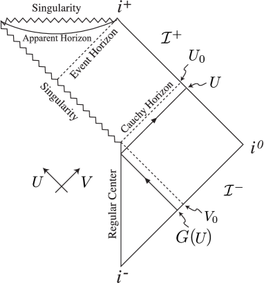
Figure 1: One of the possible causal structures considered in this article. A singularity occurs at the spacetime point $(U_{0},V_{0})$ and is visible from $\mathcal{I}^{+}$, where $(U,V)$ are suitable double null coordinates. An outgoing null ray $U=\mathrm{const.}$ can be traced backward in time from $\mathcal{I}^{+}$ to $\mathcal{I}^{-}$, which turn out to be an ingoing null ray $V=G(U)$. The outgoing null ray $U=U_{0}$ and ingoing null ray $V=V_{0}$ represent the CH and the null ray that terminates at the NS.

The regularity of the center $R=0$ in the region $v<0$ and the absence of a trapped or a marginally trapped surface for $0<R$ and $v\leq 0$ are assumed. The latter condition is $\nabla_{\mu}R\nabla^{\mu}R>0$ for all $x\in(-\infty,0]$, which is written as $g_{vv}<0$ for all $x\in(-\infty,0]$ in the present case. The inevitability of a curvature singularity at the origin $v=R=0$ can be shown except for a flat spacetime Nolan . In this article we consider self-similar spacetimes with a globally naked singularity, of which existence breaks the weak version of the cosmic censorship hypothesis. One of the possible causal structures of the naked-singular spacetimes is depicted in Fig. 1. The coordinate $v$ is set to be the proper time along the regular center to remove a gauge freedom $v\to V(v)$, so that $\lim_{x\to-\infty}g_{vv}=-1$. When $m/R^{3}$ is required to be finite at the regular center, the function $f(x)$ behaves as

$$f\simeq 2/x\;\;\mbox{as}\;\;x\to-\infty.$$ (6)

The quantity $m/R^{3}$ must be finite also in the limit $v\to 0$ for fixed $R\;(>0)$ so that

$$f=O(|x|^{\beta})\;\;\mbox{as}\;\;x\to 0,$$ (7)

where $\beta\leq-1$. When there are positive roots of the algebraic equation $f(x)=1$, it can be shown that the curve $x=x^{+}$ is a CH, as we will see in Appendix A, where $x^{+}$ is the smallest root. The differentiability of the metric function $f$ is assumed to be as follows:

$$\frac{1}{f}\in C^{0}\left((-\infty,x^{+})\right),\;\;f\in C^{2-}\;\;\mbox{at $x=x^{+}$.}$$ (8)

The former condition guarantees the existence and uniqueness of geodesics in this system. It is also assumed footnote_2 that

$$f^{\prime}(x^{+})<0.$$ (9)

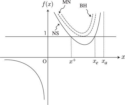
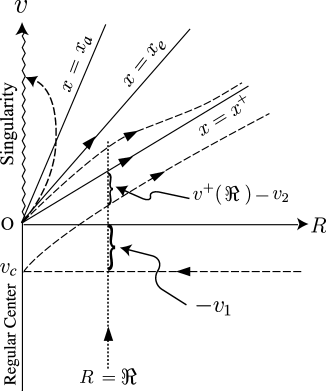
(a)	(b)

Figure 2: (a) Schematic plots of $f(x)$ defined by Eq. (3) for typical collapsing spacetimes which end in a NS or a black hole. Depending on the number of roots of $f(x)=1$, which we denote by $j$, the causal structure of spacetime changes. The cases of $j=0,\;1,\mbox{and}\;2$ are depicted. (i) The case of $j=2$ : $f(x)\,(x>0)$ is depicted by a solid line. The two roots are denoted by $x^{+}$ and $x_{e}\,\,(x^{+}<x_{e})$. The geodesics $x=x^{+}$ and $x=x_{e}$ represent the CH and event horizon, respectively. This kind of spacetime admits a NS. (ii) The case of $j=1$ : $f(x)\,(x>0)$ is depicted by a dashed line. In this case, $x^{+}=x_{e}$ holds, i.e., the CH and event horizon coincide. This type of singularity is called marginally naked (MN). (iii) The case of $j=0$ : $f(x)\,(x>0)$ is depicted by a dot-dashed line. In this case the collapse ends in a black hole (BH). (b) A typical spacetime diagram of a collapsing body which ends in a naked singularity in $(v,R)$ coordinates. A null ray which is reflected at the regular center and characteristic null rays in respective regions divided by horizons are depicted. The time intervals $v^{+}(\mathfrak{R})-v_{2}$ and $-v_{1}$ in Eq. (15) are depicted. The dotted line is the world line of an observer at $R=\mathfrak{R}$.

The schematic plot of the function $f(x)$ is shown in Fig. 2(a).

III Local Map

To estimate the power of particle creation just before the singularity occurs, the pole at $x=x^{+}$ should be extracted from the integrand in Eq. (5) as follows:

$$\frac{R}{R_{0}} = \exp\left[\int_{x_{0}}^{x}\left\{F(x^{\prime})-\frac{1}{\gamma(x^{\prime}-x^{+})}\right\}\right]\exp\left[\int_{x_{0}}^{x}\frac{dx^{\prime}}{\gamma(x^{\prime}-x^{+})}\right]$$ (10)

$$= \exp\left[\int_{x_{0}}^{x}F^{\ast}(x^{\prime})dx^{\prime}\right]\left(\frac{x^{+}-x}{x^{+}-x_{0}}\right)^{1/\gamma},$$

where

$$\gamma \equiv x^{+}f^{\prime}(x^{+}),$$ (11)

$$F^{\ast}(x) \equiv F(x)-\frac{1}{\gamma(x-x^{+})}.$$

The constant $R_{0}$ in Eq. (5), which parameterizes solutions, is related to the time $v_{c}\equiv v(R=0)<0$ when the outgoing null ray emanates from the regular center as follows:

$$\frac{R}{R_{0}} = \exp\left[-\int_{x_{0}}^{x}\frac{dx^{\prime}}{x^{\prime}}\right]\exp\left[\int_{x_{0}}^{x}\left\{F(x^{\prime})+\frac{1}{x^{\prime}}\right\}dx^{\prime}\right]$$

$$= \left|\frac{Rx_{0}}{v}\right|\exp\left[\int_{x_{0}}^{x}\frac{f(x^{\prime})}{x^{\prime}\left(f(x^{\prime})-1\right)}dx^{\prime}\right].$$

Taking the limit of $R\to 0$ $(v<0)$, following relation is obtained:

$$R_{0}=-\frac{v_{c}}{|x_{0}|I},\;\;I\equiv\exp\left[\int_{x_{0}}^{-\infty}\frac{f(x^{\prime})}{x^{\prime}\left(f(x^{\prime})-1\right)}dx^{\prime}\right],$$ (12)

where condition (6) ensures the convergence of the integral in Eq. (12).

Combination of Eqs. (10) and (12) yields

$$R=C(R,x)\left(v^{+}(R)-v\right)^{1/\gamma}v_{c},$$ (13)

where

$$v^{+}(R) \equiv x^{+}R,$$

$$C(R,x) \equiv -|x_{0}|^{-1}I^{-1}\left[(x^{+}-x_{0})R\right]^{-1/\gamma}\exp\left[\int_{x_{0}}^{x}F^{\ast}(x^{\prime})dx^{\prime}\right].$$

Before turning to the derivation of the local map, a few remarks should be made concerning the function $C(R,x)$. Due to condition (8), $C(R,x)$ converges to some finite constant in the limit $x\to x^{+}$ for fixed $R$. The dependence of $C(R,x)$ on $x_{0}$ is only an apparent one as

$$\frac{\partial C}{\partial x_{0}}=0,$$ (14)

which we use in Sec. VI.

Now let us consider a pair of ingoing and outgoing null rays such that the latter is the reflection of the former at the regular center. An observer who rests at $R=\mathfrak{R}$ will encounter the null ray twice so that we denote the time of first encounter by $v_{1}$ and that of the second by $v_{2}$. The relation between $v_{1}$ and $v_{2}$, which we call the local map, is obtained from Eq. (13):

$$v_{1}=\frac{\mathfrak{R}}{C(\mathfrak{R},x_{2})}\left(v^{+}(\mathfrak{R})-v_{2}\right)^{\alpha_{1}},$$ (15)

where

$$x_{2} \equiv v_{2}/\mathfrak{R},$$

$$\alpha_{1} \equiv -1/\gamma.$$ (16)

The time intervals $-v_{1}\;(>0)$ and $v^{+}(\mathfrak{R})-v_{2}$ are depicted schematically in Fig. 2(b). It is noted that the result does not change even if we choose a small value of $\mathfrak{R}$. Namely, the nature of the local map is determined by the behavior of null rays near the singularity.

IV Power and Energy

A global map $V=G(U)$ is defined to be a relation between the moments when one null ray leaves $\mathcal{I}^{-}$ and terminates at $\mathcal{I}^{+}$ after passing through the regular center (see Fig. 1). Assuming the geometric optics approximation, one can obtain the power of emission as the vacuum expectation value of a stress-energy tensor by the point-splitting regularization from the global map Ford ,

$$P=\frac{1}{24\pi}\left[\frac{3}{2}\left(\frac{G^{\prime\prime}}{G^{\prime}}\right)^{2}-\frac{G^{\prime\prime\prime}}{G^{\prime}}\right]$$

for a minimally coupled scalar field, and

$$\hat{P}=\frac{1}{48\pi}\left(\frac{G^{\prime\prime}}{G^{\prime}}\right)^{2}$$

for a conformally coupled scalar field.

Spherically symmetric self-similar spacetimes are not asymptotically flat in general. They therefore should be matched with an outer asymptotically flat region via a proper non-self-similar region. This matching procedure is quite straightforward for dust collapse BarveBarve2 . Although it seems to be necessary to solve null geodesic equations in such a “patched-up” spacetime, the main properties of the global map must be determined by the behavior of null rays passing near the point where the singularity occurs. This expectation has been confirmed in Tanaka , at least for the self-similar and analytic dust models. Therefore, one can safely assume that the global map inherits the main properties of the local map, such as the value of the exponent and differentiability. This means that from Eq. (15), the asymptotic form of the global map would take the form

$$G(U) = V_{0}-\left(U_{0}-U\right)^{\alpha}G_{\ast}(U),$$

where the null rays $U=U_{0}$ and $V=V_{0}$ are the CH and the ingoing null ray that terminates at the NS, respectively. The function $G_{\ast}(U)$ is a regular function which does not vanish at the CH and $\alpha$ is the exponent of the local map, $\alpha_{1}$ in Eq. (15).

In the case of $\alpha=1$, the leading contribution to the power of particle creation is calculated as

$$P = \frac{2G_{\ast}^{\prime 2}(U_{0})-G_{\ast}(U_{0})G_{\ast}^{\prime\prime}(U_{0})}{8\pi G_{\ast}^{2}(U_{0})},$$ (17)

$$\hat{P} = \frac{1}{12\pi}\left(\frac{G_{\ast}^{\prime}(U_{0})}{G_{\ast}(U_{0})}\right)^{2},$$ (18)

so that the power remains finite at the CH. Unfortunately $G_{\ast}(U_{0})$ and its derivatives cannot be known until the null geodesic equation is solved globally, so that one could not know the power of emission from only the information contained in the local map. In terms of redshift, $\alpha=1$ corresponds to the case that the redshift of a particle remains finite at the CH, as we will see in Sec. V.

On the other hand, in the case of $\alpha\neq 1$ the leading contribution is obtained as

$$P=\frac{\alpha^{2}-1}{48\pi\left(U_{0}-U\right)^{2}},$$ (19)

for a minimally coupled scalar field. For a conformally coupled one, the power of emission is obtained by replacing the factor $(\alpha^{2}-1)$ in Eq. (19) for $(\alpha-1)^{2}$. The power is proportional to the inverse square of the remaining time to the CH. If $\alpha>1$, the power diverges to positive infinity for both minimally and conformally coupled scalar fields, while if $0<\alpha<1$, the power diverges to negative and positive infinity for minimally and conformally coupled scalar fields, respectively. In terms of the redshift of particles, the case that $\alpha>1$ ($0<\alpha<1$) corresponds to infinite redshift (blueshift) at the CH, as we will see in Sec. V. The emitted energy can be estimated as

$$E=\int_{-\infty}^{U}P(U^{\prime})dU^{\prime}=\frac{\alpha^{2}-1}{48\pi\left(U_{0}-U\right)}.$$ (20)

Although the emitted energy diverges when the CH is approached, this divergence needs to be regarded carefully. The semiclassical approximation would cease to be valid when the curvature radius at some spacetime point inside star reaches the Planck scale. Here we make a natural assumption that such a situation happens at the center of a star at $v=-t_{\mathrm{QG}}$ footnote_3 . In the case of $\alpha>1$, it can be expected that for a ray emanating from the center at $v=-t_{\mathrm{QG}}$, the time difference $U_{0}-U$ would be greater than the order of $t_{\mathrm{QG}}$ due to redshift, i.e., $\Delta U\equiv U_{0}-U>t_{\mathrm{QG}}$. Then energy emitted by the time $U_{0}-\Delta U$ is

$$E=\frac{\alpha^{2}-1}{48\pi\Delta U}<\frac{\alpha^{2}-1}{48\pi}E_{\mathrm{QG}},$$ (21)

where $E_{\mathrm{QG}}\equiv 1/t_{\mathrm{QG}}$. If the factor $\left(\alpha^{2}-1\right)/(48\pi)$ is on the order of unity, the total radiated energy within the semiclassical phase is less than the order of $E_{\mathrm{QG}}$, which would be of course much less than the mass of ordinary astrophysical stars. It would be better to say that a collapsing star would enter the phase of quantum gravity with most of its mass intact. Therefore, one could not predict whether a star which collapses to a NS evaporates away or ceases to radiate at its final epoch. This has been pointed out in NSEandQG after careful investigation. We should not overlook that this feature is much different from that of black hole evaporation, in which quantum gravitational effects appear after a black hole loses almost all its mass.

One can recognize, however, that if $\alpha\gg 1$ the radiated energy could be large. This situation is realized in the limit to marginally NS, in which the CH and event horizon coincide footnote_4 . To illustrate the unbounded increase of $\alpha$ in this limit, we have to look deeper into the causal structure, which is determined by the function $f$. We order the positive roots of the equation $f(x)=1$ as $0<x_{1}=x^{+}<x_{2}<\cdot\cdot\cdot<x_{n}$, where we count multiple roots as one root. The existence of $x_{a}$ satisfying $\lim_{x\to x_{a}}f(x)=+\infty$ with $x_{n}<x_{a}$ and the continuity of $f$ in the region $x_{1}<x<x_{a}$ are assumed. In the region $x\in\left(x_{n},x_{a}\right)$, $dR/dv>0$ along the null geodesics and $\lim_{x\to x_{a}}dR/dv=0$ from Eq. (2). This implies that outgoing null rays in this region are to turn back in the direction of the singularity at $x=x_{a}$ and that the curve $x=x_{n}$ is the last outgoing null ray which can escape to infinity. That is to say, $x=x_{a}$ and $x=x_{n}\equiv x_{e}$ are the apparent horizon and event horizon, respectively. Hereafter, we shall concentrate on the case of $n=2$. The function $f(x)$ would be written as

$$f(x)-1=f_{\ast}(x)(x-x^{+})\left(x_{e}-x\right)^{m},\;\;0<x<x_{a},$$ (22)

where $f_{\ast}(x)$ is a function which satisfies $f_{\ast}(x^{+})<0$ and $m$ is some positive integer. The exponent of the factor $(x-x^{+})$ is restricted to unity because of the condition $f^{\prime}(x^{+})<0$ and the differentiability $f\in C^{2-}$ at $x=x^{+}$. With Eq. (22), the exponent of the local map is calculated as

$$\alpha_{1}\equiv-\frac{1}{x^{+}f^{\prime}(x^{+})}=-\frac{1}{x^{+}f_{\ast}^{\prime}(x^{+})\left(x_{e}-x^{+}\right)^{m}},$$ (23)

to show that $\alpha_{1}$ can be arbitrarily large in the limit $x^{+}\to x_{e}$.

V Redshift

The estimation of redshift of the radial null ray would help us understand the behavior of the power and would be necessary for discussing the validity of geometric optics and semiclassical approximations. Hereafter the tangent vector of the null ray is denoted by $k^{\mu}\equiv dx^{\mu}/d\lambda$, where $\lambda$ is an affine parameter.

With the null condition $k^{\mu}k_{\mu}=0$, the $v$-component of the geodesic equation $k^{\mu}\nabla_{\mu}k^{\nu}=0$ leads to

$$\frac{dk^{v}}{d\lambda}+\frac{(k^{v})^{2}}{R}\left(\frac{1}{g_{vR}}\frac{dg_{vR}}{dx}+\frac{x}{2}\frac{1}{g_{vR}}\frac{dg_{vv}}{dx}\right)=0.$$

Furthermore by using the relation

$$\frac{d}{d\lambda}=\frac{k^{v}}{R}\left(1+\frac{xg_{vv}}{2g_{vR}}\right)\frac{d}{dx},$$

$k^{v}(x)$ is integrated to give

$$\frac{k^{v}(x)}{k^{v}_{0}}=\exp\left[\int^{x}_{\tilde{x}_{0}}\tilde{F}(x^{\prime})dx^{\prime}\right]=\exp\left[\int_{\tilde{x}_{0}}^{x}\tilde{F}^{\ast}(x^{\prime})dx^{\prime}\right]\left(\frac{x^{+}-x}{x^{+}-\tilde{x}_{0}}\right)^{-(1+\gamma)/\gamma},$$ (24)

where

$$\tilde{F}(x) \equiv -\frac{1}{g_{vR}}\frac{dg_{vR}}{dx}+\frac{1}{1-f}\left(\frac{1}{x}+\frac{1}{f}\frac{df}{dx}\right),$$

$$\tilde{F}^{\ast}(x) \equiv \tilde{F}(x)+\frac{1+\gamma}{\gamma}\frac{1}{x-x^{+}}.$$

The constant $\tilde{x}_{0}$, which is set as $\tilde{x}_{0}<x^{+}$, and the constant $k^{v}_{0}$ are related as $k^{v}_{0}=k^{v}(\tilde{x}_{0})$.

The constant $k^{v}_{0}$ is related to $k^{v}_{c}\equiv k^{v}(R=0)$ as

$$k^{v}_{0}=\frac{k^{v}_{c}}{\tilde{I}},\;\;\tilde{I}\equiv\exp\left[\int^{-\infty}_{\tilde{x}_{0}}\tilde{F}(x^{\prime})dx^{\prime}\right].$$ (25)

Combination of Eqs. (24) and (25) yields

$$k^{v}(x)=\tilde{C}(R,x)\left(v^{+}(R)-v\right)^{\alpha_{1}-1}k^{v}_{c},$$ (26)

where

$$\tilde{C}(R,x)\equiv\tilde{I}^{-1}\left[(x^{+}-\tilde{x}_{0})R\right]^{(1+\gamma)/\gamma}\exp\left[\int_{\tilde{x}_{0}}^{x}\tilde{F}^{\ast}(x^{\prime})dx^{\prime}\right].$$

Now, let us consider time-like observers who rest at $R=0$ and $R=\mathfrak{R}\;(d\theta=d\phi=0)$. The observed frequency is given by $\hat{\omega}\equiv-u_{\mu}k^{\mu}=\sqrt{|g_{vv}(x)|}k^{v}(x)$, where $u_{\mu}$ is the four-velocity of observer. When $\hat{\omega}_{1}\equiv\lim_{x\to-\infty}\hat{\omega}(x)$ and $\hat{\omega}_{2}\equiv\lim_{x\to x^{+}}\hat{\omega}(x)$ are defined, Eq. (26) yields

$$\frac{\hat{\omega}_{2}}{\hat{\omega}_{1}}=\sqrt{\left|\frac{g_{vv}(x^{+})}{g_{vv}(-\infty)}\right|}\tilde{C}(\mathfrak{R},x_{2})(v^{+}(\mathfrak{R})-v_{2})^{\alpha_{1}-1}.$$ (27)

Thus we see that if $\alpha_{1}>1$ ($0<\alpha_{1}<1$) the redshift (blueshift) of emitted particle diverges at the CH, while it remains finite if $\alpha_{1}=1$. The relation between the redshift derived above and the local map will be presented in the next section.

VI Relations among the Local Map, Power, and Redshift

There would be a relation between the local map and redshift because the local map describes a kind of time delay. Since the asymptotic behavior of the local map and redshift in the limit $x\to x^{+}$ is considered here, the time dependence is omitted as $C(R,x)\to C(R)$. From Eq. (15), the relation

$$\frac{dv_{2}}{dv_{1}}=\frac{\gamma C(\mathfrak{R})}{\mathfrak{R}}(v^{+}(\mathfrak{R})-v_{2})^{(1+\gamma)/\gamma}$$ (28)

holds to give an alternative definition of redshift. Indeed, the time dependence in Eq. (28) can be replaced with the ratio of $k^{v}$ by Eq. (26) as

$$\frac{dv_{2}}{dv_{1}}=\left|\frac{g_{vv}(-\infty)}{g_{vv}(x^{+})}\right|\frac{k^{v}_{c}}{k^{v}(x_{2})},$$ (29)

where we set $x_{0}=\tilde{x}_{0}$ in the evaluation of the integral in $C$ to derive Eq. (29) since $C$ does not depend on $x_{0}$ from Eq. (14). Equation (29) can be written as

$$\frac{d\tau_{2}}{d\tau_{1}}=\frac{\hat{\omega}_{1}}{\hat{\omega}_{2}},$$ (30)

where $d\tau_{i}\equiv\sqrt{|g_{vv}|}dv_{i}$ $(i=1,2)$ is the proper time measured by the observer. This relates the time delay and redshift to reveal that the redshift essentially corresponds to the local map and also to confirm the consistency of the analyses in Secs. III and V.

There exists a plausible relation also between the power of emission and the redshift of particles as mentioned in Sec. IV. In the case of $\alpha>1$ ($0<\alpha<1$), the power and redshift (blueshift) diverge at the CH from Eqs. (19) and (27), while the power and redshift remain finite at the CH in the case of $\alpha=1$. We may, therefore, reasonably conclude that the divergence of the redshift or blueshift at the CH causes that of the power.

VII Examples

In this section, we will take examples to illustrate how the features obtained in the previous sections are realized in concrete models. Since several models are written in the diagonal form of a metric tensor, the formulation and notations for the diagonal form of a metric tensor are developed in Appendix B.

VII.1 Minkowski spacetime

Although neither singularity nor horizon exists in Minkowski spacetime, one can test the formalism by applying it to this trivial spacetime. The line element is written as

$$ds^{2}=-dv^{2}+2dvdR+R^{2}d\Omega^{2},$$

or

$$ds^{2}=-dt^{2}+dr^{2}+r^{2}d\Omega^{2}.$$

From definitions (3) and (38), one obtains

$$f(x)=\frac{2}{x},\;\;w_{\pm}(z)=\pm\frac{1}{z}.$$

The roots of the algebraic equations $f(x)=1$ and $w_{\pm}(z)=1$ are given as $x^{+}=2$ and $z^{\pm}=\pm 1$, respectively. It must be noted that the function $f(x)$ satisfies conditions (6)-(9), which have been assumed to derive the local map. According to Eqs. (11), (16), (40), and (44), one can easily check that the exponents of local maps, $\alpha_{1}$ and $\alpha_{2}$, are unity. This fact just tells us that the redshift and power remain finite in a flat spacetime.

VII.2 Vaidya Solution

The Vaidya solution describes the collapse of a null-dust fluid Vaidya_1Vaidya_2Vaidya_3 . The global map for the self-similar Vaidya collapse was derived in Singh .

The line element in the self-similar Vaidya spacetime is written as

$$ds^{2}=-\left(1-m(x)\right)dv^{2}+2dvdR+R^{2}d\Omega^{2},$$

where $m(x)=0$ for $x<0$ and $m(x)=2\mu x$ for $x\geq 0$. The constant $\mu$ is restricted as $0<\mu<1/16$ for the nakedness, so that the spacetime with $\mu=1/16$ corresponds to a marginally naked-singular one. The function $f(x)$ is written as

$$f(x)=\frac{2}{x(1-m(x))}.$$

The roots of algebraic equation $f(x)=1$ are given as

$$x^{+}=\frac{1-\sqrt{1-16\mu}}{4\mu}\quad\mbox{and}\quad x_{e}=\frac{1+\sqrt{1-16\mu}}{4\mu}.$$

What has to be noticed is that $f$ satisfies conditions (6)-(9). The exponent is calculated as

$$\alpha_{1}\equiv-\frac{1}{x^{+}f^{\prime}(x^{+})}=\frac{1+\sqrt{1-16\mu}}{2\sqrt{1-16\mu}}.$$

This exponent coincides with that of the global map which was obtained in Singh . One can see that $\lim_{\mu\to 0}\alpha_{1}=1$ and $\lim_{\mu\to 1/16}\alpha_{1}=\infty$, where the former and latter correspond to the limits of Minkowski and marginally naked-singular spacetime. This example is a good illustration of the efficiency of the local map and the divergence of $\alpha_{1}$ in the limit to marginally NS.

VII.3 Roberts Solution

The Roberts solution describes the self-similar collapse of a massless scalar field Roberts . The line element is given as

$$ds^{2}=-\left(1-\frac{2h(x)h^{\prime}(x)}{\sqrt{1+h^{2}(x)}}\right)dv^{2}+\frac{2}{\sqrt{1+h^{2}(x)}}dvdR+R^{2}d\Omega^{2},$$ (31)

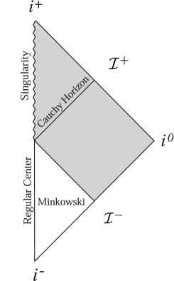
Figure 3: The conformal diagram of the Roberts solution Eq. (31) with $|\sigma|<1/2$. The region $v<0$ is flat and the shading region is filled with a collapsing massless scalar field. A time-like NS occurs at $v=0$.

where $h(x)=0$ for $x<0$ and $h(x)=\sigma x$ for $x\geq 0$, so that the region with negative $v$ is flat. The constant $\sigma$ is restricted here as $|\sigma|<1/2$ for the causal structure such that the spacetime has a time-like NS as in Fig. 3. The function $f(x)$ is written as

$$f(x)=\frac{2}{x(\sqrt{1+h^{2}}-2hh^{\prime})}.$$

The conditions on $f(x)$ are again satisfied. The algebraic equation $f(x)=1$ has a positive root $x^{+}=2/\sqrt{1-4\sigma^{2}}$ so that the exponent of local map is calculated as

$$\alpha_{1}\equiv-\frac{1}{x^{+}f^{\prime}(x^{+})}=1$$

for $|\sigma|<1/2$. Thus we see that the Roberts solution provides a non-trivial example of spacetime in which the power of particle creation remains finite at the CH in self-similar collapse.

VII.4 Lemaître-Tolman-Bondi Solution

The Lemaître-Tolman-Bondi (LTB) solution describes the collapse of a dust fluid LemaitreTolmanBondi . Although both global and local maps were derived in BarveBarve2 and Tanaka respectively for self-similar LTB collapse, the exponent in BarveBarve2 is reproduced from the formalism in Sec. III.

The line element of self-similar LTB spacetime (for example, see BarveBarve2 ) is

$$ds^{2}=-dt^{2}+\left[\frac{1-az/3}{(1-az)^{1/3}}\right]^{2}dr^{2}+r^{2}(1-az)^{4/3}d\Omega^{2},$$

where the constant $a$ is related to a “mass parameter” $\lambda$ as $a=\frac{3}{2}\sqrt{\lambda}$. The constant $\lambda$ is restricted to the range $0<\lambda<6(26-15\sqrt{3})\equiv\lambda_{m}$, where the latter inequality is imposed by the nakedness of the singularity Joshi , so that the spacetime with $\lambda=\lambda_{m}$ corresponds to marginally naked-singular one. One obtains the function $w_{\pm}(z)$ according to definition (38) as

$$w_{\pm}(z)=\pm\frac{1-az/3}{z\left(1-az\right)^{1/3}}.$$ (32)

The required conditions on $w_{\pm}$ in calculating the local map are satisfied. When a new variable $y\equiv\left(1-az\right)^{1/3}$ introduced, Eq. (32) can be written as

$$w_{\pm}^{2}(z)=1-\frac{4g_{+}(y)g_{-}(y)}{\left[g_{+}(y)+g_{-}(y)\right]^{2}},$$

where $g_{\pm}(y)\equiv 3y^{4}\mp ay^{3}-3y\mp 2a$, so that the roots of algebraic equations $w_{\pm}(z)=1$ correspond to those of $g_{\mp}(y)=0$. Using the chain rule $d/dz=(dy/dz)d/dy$, one obtains

$$z^{\pm}w_{\pm}^{\prime}(z^{\pm})=\frac{2(1-3\alpha_{\mp}^{3})g^{\prime}_{\mp}(\alpha_{\mp})}{3\alpha_{\pm}g_{\pm}(\alpha_{\mp})},$$

where $\alpha_{\pm}\equiv\left(1-az^{\mp}\right)^{1/3}$ and the prime denotes differentiation with respect to the argument of the function. The exponent of local map is calculated as

$$\alpha_{2}\equiv\frac{z^{-}w_{-}^{\prime}(z^{-})}{z^{+}w_{+}^{\prime}(z^{+})}=\frac{\alpha_{-}^{3}g^{\prime}_{+}(\alpha_{+})}{\alpha_{+}^{3}g^{\prime}_{-}(\alpha_{-})}$$

to coincide with the one derived in BarveBarve2 ; Tanaka . This exponent becomes close to unity as $\lambda\to 0$ and increases monotonically with $\lambda$ to diverge to infinity as $\lambda\to\lambda_{m}$.

VII.5 General Relativistic Larson-Penston Solution

As the last example the general relativistic Larson-Penston (GRLP) solution, which describes the self-similar collapse of a perfect fluid OriPiran3 ; OriPiranOriPiran2 , is considered. For the present, it may be useful to review the GRLP solution and its importance, although we have mentioned them in the Introduction. The equation of state must have the form of $P=k\rho$ from the requirement of self-similarity, where $k$ is a constant. The GRLP solution represents a naked-singularity formation in the range $0<k\lesssim 0.0105$, where the upper bound is imposed by the nakedness of the singularity. This solution is interesting because it provides the first example in which the pressure does not prevent the formation of a NS. Moreover, the convergence to the GRLP solution of more general solutions near the central region of stars have been strongly suggested numerically and supported by a mode analysis HaradaMaeda as a realization of the self-similarity hypothesis Carr . From the above, the GRLP solution will be a strongest known counterexample against the cosmic censorship hypothesis.

Because the GRLP solution is a numerical one, an explicit expression of the exponent of local map could not obtained analytically, although it is unlikely that $\alpha$ is equal to unity. To show rigorously that the power of emission is proportional to the inverse square of the remaining time to the CH and that the constant of proportion diverges in the limit to marginally NS, the dependence of exponent $\alpha$ on $k$ should be clarified numerically preparation .

VIII Summary and Discussion

We have been concerned with a quantum mechanical particle creation during the naked-singularity formation in spherically symmetric self-similar collapse. The power, energy, and redshift of emitted particles are analytically calculated on the assumption that the curvature around the singularity causes particle creation and the metric function $f$ is $C^{2-}$ around the CH. As a result, in the generic case in which the exponent of the local map $\alpha\neq 1$, the power has been found to diverge as $P\varpropto(t_{ch}-t)^{-2}$, where $(t_{ch}-t)$ is the remaining time until a distant observer would receive a first light ray from the NS. It is worth pointing out that the weaker differentiability of the CH leads to a different result, i.e., the power of emission has a different time dependence, although we have not looked deeper into such a possibility in this paper. The square inverse proportion of the power to the remaining time is due to the scale invariance of self-similar spacetimes. The constant of proportion has been found to be arbitrarily large in the limit to marginally NS. Therefore, this explosive radiation is especially striking in the case that the event horizon is very close to the CH because the emitted energy can be arbitrarily large in spite of a cutoff expected from quantum gravity. We go on from this to the conclusion that if the back reaction to a gravitational field is taken into account, the semiclassical effect would cause the instability of the CH and might recover the cosmic censor in this limiting case. On the other hand, in the non-generic case in which $\alpha=1$ the power remains finite at the CH, so that the semiclassical instability of the CH seems not to be efficient for this special class of self-similar solutions. The collapse of a massless scalar field described by the Roberts solution indeed does correspond to this case. In addition, it has been found that the diverging redshift and blueshift cause the divergence of the power to positive or negative infinity, depending on the manner of the coupling of scalar fields to gravity. The divergence will be a criterion for the stability/instability of a CH in a gravitational collapse. Having suggested that the particle creation could cause the instability of the CH, we still have a long way to go before knowing the existence of a classical/semiclassical cosmic censor in more generic spacetimes.

Appendix A First outgoing null ray from the singularity

We shall prove the absence of an outgoing radial null geodesic which emanates from the origin $v=R=0$ before the null geodesic $x=x^{+}$. Let $(v,R)$ be a point on a radial null geodesic $l$ in the region $0<x=v/R<x^{+}$ which emanates from $v=R=0$. Then, one can say that

$$\left.\frac{dx}{dv}\right|_{l}=\frac{x}{v}(1-\frac{1}{f})>0.$$ (33)

By the uniqueness of the solution of the null geodesic equation, $l$ cannot cross $x=x^{+}$ at points other than $v=R=0$. Therefore above inequality says that $x$ decreases as $v\to+0$ but is bounded from below by $0$. Hence the limit

$$\bar{x}\equiv\left.\lim_{v\to+0}x(v)\right|_{l}$$ (34)

exists and satisfies $0\leq\bar{x}<x^{+}$. In the case of $0<\bar{x}<x^{+}$,

$$\bar{R}\equiv\left.\lim_{v\to+0}R(v)\right|_{l}\\ =\left.\lim_{v\to+0}\frac{v}{x(v)}\right|_{l}\\ =0$$ (35)

holds, but

$$\bar{x}=\left.\lim_{v\to+0}\frac{v}{R(v)}\right|_{l}=\left.\lim_{v\to+0}\frac{1}{R^{\prime}(v)}\right|_{l}=\left.\lim_{v\to+0}xf(x)\right|_{l}=\bar{x}f(\bar{x}),$$ (36)

where the l’Hopital’s rule is used in the second equality. This contradicts the assumption that $x^{+}$ is the smallest positive root of equation $f(x)=1$. Next, we shall consider the case of $\bar{x}=0$. The fact that the solution $R$ converges to a finite nonzero constant as $x\to 0$ from the condition (7) contradicts the assumption that $l$ is a geodesic which emanates from $v=R=0$. Thus the case of $\bar{x}=0$ is also excluded. Thus we see that $x=x^{+}$ is the first outgoing null ray which emanates from the singularity.

Appendix B Local Map and Redshift in Diagonal Coordinates

The line element of the class of spacetimes discussed in Sec. II in a diagonal coordinate system is written as

$$ds^{2}=g_{tt}(z)dt^{2}+g_{rr}(z)dr^{2}+r^{2}S^{2}(z)d\Omega^{2},$$ (37)

where $z\equiv t/r$ and $S$ is a dimensionless metric function. The homothetic Killing vector field is of the form $\xi=t\partial_{t}+r\partial_{r}$. If one defines functions $w_{\pm}(z)$ as

$$w_{\pm}(z)\equiv\pm\frac{1}{z}\sqrt{-\frac{g_{rr}}{g_{tt}}},$$ (38)

the roots of the algebraic equation $w_{\pm}(z)=1$ play important roles as do those of $f(x)=1$ in Sec. II. The existence of a positive (negative) root of $w_{+}(z)=1$ ($w_{-}(z)=1$) and the uniqueness of the root of $w_{-}(z)=1$ are assumed. When the negative root and the smallest positive root are denoted by $z^{-}$ and $z^{+}$ respectively, the curves $z=z^{+}$ and $z=z^{-}$ can be shown to be the CH and the ingoing null ray that terminates at the NS. In addition, it is assumed that $w^{\prime}_{\mp}(z^{\mp})\gtrless 0$.

The null geodesic equations are integrated to give

$$\frac{r}{r_{0}^{\pm}}=\exp\left[\int_{z_{0}^{\pm}}^{z}W_{\pm}(z^{\prime})dz^{\prime}\right]=\exp\left[\int_{z_{0}^{\pm}}^{z}W^{\ast}_{\pm}(z^{\prime})dz^{\prime}\right]\left(\frac{z^{\pm}-z}{z^{\pm}-z_{0}^{\pm}}\right)^{1/\delta_{\pm}},$$ (39)

where

$$W_{\pm}(z) \equiv \frac{1}{z\left(w_{\pm}(z)-1\right)},$$

$$\delta_{\pm} \equiv z^{\pm}w_{\pm}^{\prime}(z^{\pm}),$$ (40)

$$W^{\ast}_{\pm}(z) \equiv W_{\pm}(z)-\frac{1}{\delta_{\pm}(z-z^{\pm})},$$

and the signature $+$ $(-)$ corresponds to outgoing (ingoing) null geodesic. The constants $z_{0}^{\pm}$ and $r_{0}^{\pm}$ are related as $r_{0}^{+}=r(z=z_{0}^{+})$ for an outgoing ray, while $r_{0}^{-}=r(z=z_{0}^{-})$ for an ingoing one, where $z_{0}^{\pm}$ is set as $z_{0}^{\pm}<z^{\pm}$ and $z_{0}^{\pm}\neq 0$. The constants $r^{\pm}_{0}$ are related to $t_{c}\equiv t(r=0)$ as

$$r_{0}^{\pm}=-\frac{t_{c}}{|z_{0}^{\pm}|J_{\pm}},\;\;J_{\pm}=\exp\left[\int_{z_{0}^{\pm}}^{-\infty}\frac{w_{\pm}(z^{\prime})dz^{\prime}}{z^{\prime}\left(w_{\pm}(z^{\prime})-1\right)}\right].$$ (41)

Combination of Eqs. (39) and (41) yields

$$r = D_{\pm}(r,z)\left(t^{\pm}(r)-t\right)^{1/\delta_{\pm}}t_{c},$$ (42)

where

$$t^{\pm}(r) \equiv z^{\pm}r,$$

$$D_{\pm}(r,z) \equiv -|z_{0}^{\pm}|^{-1}J_{\pm}^{-1}\left[(z^{\pm}-z_{0}^{\pm})r\right]^{-1/\delta_{\pm}}\exp\left[\int_{z_{0}^{\pm}}^{z}W_{\pm}^{\ast}(z^{\prime})dz^{\prime}\right].$$

Now, let us consider a pair of ingoing and outgoing null rays such that the latter is the reflection of the former at the regular center $(r=0,t<0)$. An observer who rests at $r=\mathfrak{r}$ will encounter the null ray twice, so that we denote the time of first encounter by $t_{1}$ and that of the second by $t_{2}$. By Eq. (42), the ingoing and outgoing null rays are matched at the center to give the local map as

$$t^{-}(\mathfrak{r})-t_{1}=\left[\frac{D_{+}(\mathfrak{r},z_{2})}{D_{-}(\mathfrak{r},z_{1})}\right]^{\delta_{-}}\left(t^{+}(\mathfrak{r})-t_{2}\right)^{\alpha_{2}},$$ (43)

where

$$z_{i} \equiv t_{i}/\mathfrak{r},\,\,(i=1,2),$$

$$\alpha_{2} \equiv \delta_{-}/\delta_{+}.$$ (44)

The redshift of a radial null ray is obtained in similar way. The $t$-component of equation $k^{\mu}\nabla_{\mu}k^{\nu}=0$ is integrated to give

$$\frac{k^{t}(z)}{k^{t,\pm}_{0}}=\exp\left[\int_{\tilde{z}_{0}^{\pm}}^{z}\tilde{W}_{\pm}(z^{\prime})dz^{\prime}\right]=\exp\left[\int_{\tilde{z}_{0}^{\pm}}^{z}\tilde{W}_{\pm}^{\ast}(z^{\prime})dz^{\prime}\right]\left(\frac{z^{\pm}-z}{z^{\pm}-\tilde{z}_{0}^{\pm}}\right)^{-(1+\delta_{\pm})/\delta_{\pm}},$$ (45)

where

$$\tilde{W}_{\pm}(z) \equiv -\frac{1}{2\left(1-w_{\pm}^{-1}\right)}\left\{\left(1-2w^{-1}_{\pm}\right)\frac{1}{g_{tt}}\frac{dg_{tt}}{dz}+\frac{1}{g_{rr}}\frac{dg_{rr}}{dz}\right\},$$

$$\tilde{W}_{\pm}^{\ast}(z) \equiv \tilde{W}_{\pm}(z)+\frac{1+\delta_{\pm}}{\delta_{\pm}}\frac{1}{z-z^{\pm}}.$$

The constants $\tilde{z}_{0}^{\pm}$ and $k^{t,\pm}_{0}$ are related as $k^{t,+}_{0}=k^{t}(z^{+}_{0})$ for an outgoing ray, while $k^{t,-}_{0}=k^{t}(z^{-}_{0})$ for an ingoing one. The constants $k^{t,\pm}_{0}$ are related to $k^{t}_{c}\equiv k^{t}(r=0)$ as

$$k^{t,\pm}_{0}=\frac{k^{t}_{c}}{\tilde{J}_{\pm}},\;\;\tilde{J}_{\pm}\equiv\exp\left[\int_{\tilde{z}_{0}^{\pm}}^{-\infty}\tilde{W}_{\pm}(z^{\prime})dz^{\prime}\right].$$ (46)

Combination of Eqs. (45) and (46) yields

$$k^{t}(z)=\tilde{D}_{\pm}(r,z)\left(t^{\pm}(r)-t\right)^{-(1+\delta_{\pm})/\delta_{\pm}}k^{t}_{c},$$ (47)

where

$$\tilde{D}_{\pm}(r,z)\equiv\tilde{J}_{\pm}^{-1}\left[(z^{\pm}-\tilde{z}_{0}^{\pm})r\right]^{(1+\delta_{\pm})/\delta_{\pm}}\exp\left[\int_{\tilde{z}_{0}^{\pm}}^{z}\tilde{W}^{\ast}_{\pm}(z^{\prime})dz^{\prime}\right].$$

Consider again the observer who rests at $r=\mathfrak{r}$ and the pair of ingoing and outgoing null rays. The outgoing and ingoing null rays are matched at the center by Eqs. (43) and (47) to give

$$\frac{\hat{\omega}_{2}}{\hat{\omega}_{1}}=\sqrt{\left|\frac{g_{tt}(z^{+})}{g_{tt}(z^{-})}\right|}\frac{\tilde{D}_{+}(\mathfrak{r},z_{2})}{\tilde{D}_{-}(\mathfrak{r},z_{1})}\left[\frac{D_{+}(\mathfrak{r},z_{2})}{D_{-}(\mathfrak{r},z_{1})}\right]^{1+\delta_{-}}\left(t^{+}(\mathfrak{r})-t_{2}\right)^{\alpha_{2}-1},$$ (48)

where $\hat{\omega}_{1}\equiv\lim_{z_{1}\to z^{-}}\sqrt{|g_{tt}(z_{1})|}\,k^{t}(z_{1})$ and $\hat{\omega}_{2}\equiv\lim_{z_{2}\to z^{+}}\sqrt{|g_{tt}(z_{2})|}\,k^{t}(z_{2})$ are the observed frequencies.

There exists a plausible relation between the local map and redshift. From Eqs. (43) and (48), one obtains

$$\frac{d\tau_{2}}{d\tau_{1}}=\frac{\hat{\omega}_{1}}{\hat{\omega}_{2}},$$

where $d\tau_{i}\equiv\sqrt{|g_{tt}|}\,dt_{i}$ ($i=1,2$) is the proper time of the observers.

References

- (1) R. Penrose, Riv. Nuovo Cim. 1, 252 (1969), reprinted in Gen. Relat. Grav. 34, 1141 (2002); in General Relativity, An Einstein Century Survey, edited by S. W. Hawking and W. Israel (Cambridge University Press, Cambridge, England, 1979), p. 581.
- (2) S. W. Hawking, Commun. Math. Phys. 43,199 (1975).
- (3) L. H. Ford and L. Parker, Phys. Rev. D 17, 1485 (1978).
- (4) W. A. Hiscock, L. G. Williams, and D. M. Eardley, Phys. Rev. D 26, 751 (1982).
- (5) S. Barve, T. P. Singh, C. Vaz, and L. Witten, Nucl. Phys. B 532, 361 (1998); Phys. Rev. D 58, 104018 (1998).
- (6) C. Vaz and L. Witten, Phys. Lett. B 442, 90 (1998) .
- (7) T. Harada, H. Iguchi, K. Nakao, Phys. Rev. D 61, 101502 (2000); ibid. 62, 084037 (2000).
- (8) T. P. Singh and C. Vaz, Phys. Lett. B 481, 74 (2000).
- (9) T. Harada, H. Iguchi and K. Nakao, Prog. Theor. Phys. 107, 449 (2002).
- (10) P. S. Joshi, N. Dadhich, and R. Maartens, Mod. Phys. Lett. A 15, 991 (2000).
- (11) B. Waugh and K. Lake, Phys. Rev. D 40, 2137 (1989).
- (12) K. Lake and T. Zannias, Phys. Rev. D 41, 3866 (1990).
- (13) A. Ori and T. Piran, Phys. Rev. D 42, 1068 (1990).
- (14) A. Ori and T. Piran, Phys. Rev. Lett. 59, 2137 (1987); Gen. Relat. Grav. 20, 7 (1988).
- (15) T. Harada and H. Maeda, Phys. Rev. D 63, 084022 (2001).
- (16) B. J. Carr and A. A. Coley, Class. Quantum. Grav. 16, R31 (1999).
- (17) B. J. Carr, in Proceedings of the Ninth Workshop on General Relativity and Gravitation, 1999, edited by Y. Eriguchi et al. (Hiroshima, Japan), p. 425, gr-qc/0003009.
- (18) C. Gundlach, Phys. Rep. 376, 339 (2003).
- (19) T. Tanaka and T. P. Singh, Phys. Rev. 63, 124021 (2001) .
- (20) B. C. Nolan and T. Waters, Phys. Rev. D 66, 104012 (2002).
- (21) One can prove with the dominant energy condition on collapsing matter and the equality is excluded by a physically reasonable requirement on the collapsing matter at the CH Nolan .
- (22) The time can be regarded as the Planck time ; at least this is the case for self-similar dust model.
- (23) T. Harada, H. Iguchi, K. Nakao, T. Tanaka, T.P. Singh and C. Vaz, Phys. Rev. D 64, 041501 (2001).
- (24) When the CH and event horizon exactly coincide, radiation reduces to the Hawking one Ford ; Hiscock . This fact cannot be derived with the method making use of the local map since in this case, in Eq. (10). It is not surprising since an event horizon, which plays a central role in the Hawking radiation, is not a local object but a global one.
- (25) P. C. Vaidya, Current Science 13, 183 (1943); Phys. Rev. 47, 10 (1951); Proc. Indian Acad. Sci. A 33, 264 (1951).
- (26) M. D. Roberts, Gen. Rel. Grav. 21, 907 (1989).
- (27) G. Lemaître, Ann. Soc. Sci. Bruxelles I A 53, 51 (1933); R. C. Tolman, Proc. Nat. Acad. Sci. 20, 169 (1934); H. Bondi, Mon. Not. R. Astron. Soc. 107, 410 (1947).
- (28) P. S. Joshi and I. H. Dwivedi, Phys. Rev. D 47, 5357 (1993).
- (29) U. Miyamoto and T. Harada (in preparation).