Isotropic singularity in inhomogeneous brane cosmological models

Abstract

We discuss the asymptotic dynamical evolution of spatially inhomogeneous brane-world cosmological models close to the initial singularity. By introducing suitable scale-invariant dependent variables and a suitable gauge, we write the evolution equations of the spatially inhomogeneous $G_{2}$ brane cosmological models with one spatial degree of freedom as a system of autonomous first-order partial differential equations. We study the system numerically, and we find that there always exists an initial singularity, which is characterized by the fact that spatial derivatives are dynamically negligible. More importantly, from the numerical analysis we conclude that there is an initial isotropic singularity in all of these spatially inhomogeneous brane cosmologies for a range of parameter values which include the physically important cases of radiation and a scalar field source. The numerical results are supported by a qualitative dynamical analysis and a calculation of the past asymptotic decay rates. Although the analysis is local in nature, the numerics indicates that the singularity is isotropic for all relevant initial conditions. Therefore this analysis, and a preliminary investigation of general inhomogeneous ($G_{0}$) models, indicates that it is plausible that the initial singularity is isotropic in spatially inhomogeneous brane-world cosmological models and consequently that brane cosmology naturally gives rise to a set of initial data that provide the conditions for inflation to subsequently take place.

I Introduction

String inspired theories in which the matter fields are confined to a 3-dimensional ‘brane-world’ embedded in $1+3+d$ dimensions while the gravitational field can also propagate in the $d$ extra dimensions [1] are currently of great interest. In particular, Randall and Sundrum [2] have shown that for $d=1$, gravity can be localized on a single 3-brane at lower energies even when the fifth dimension is infinite. The Randall-Sundrum type models are simple phenomenological models, which capture some of the essential features of the dimensional reduction of eleven-dimensional supergravity introduced by Ho$\check{\mbox{r}}$ava and Witten [3]. An elegant geometric formulation and generalization of the Randall-Sundrum-type brane-world models has been given [4, 5]. Recently there has been great interest in Randall-Sundrum-type brane-world cosmological models [2], particularly in an attempt to understand the dynamics of the universe at early times. Brane-world models have a different qualitative behaviour than their general-relativistic counterpart [6, 4], especially at high energies when the energy density of the matter is larger than the brane tension and the behaviour deviates significantly from the classical case.

The asymptotic dynamical evolution of spatially homogeneous brane-world cosmological models close to the initial singularity was studied in [7]. It was found that an isotropic singularity [8] is a past-attractor in all orthogonal Bianchi models and is a local past-attractor in a class of inhomogeneous brane-world models (and consequently these models do not exhibit Mixmaster or chaotic-like behaviour close to the initial singularity). However, the study of the behaviour of spatially homogeneous brane-worlds close to the initial singularity in the presence of both local and nonlocal stresses indicates that for physically relevent values of the equation of state parameter there exist two local past attractors for these brane-worlds, one isotropic past attractor and one anisotropic past attractor; i.e., in these brane-worlds the initial singularity can be locally either isotropic or anisotropic [9, 10] (however, the anisotropic models appear to be unphysical and can likely be ruled out). Therefore, it is plausible that typically the initial singularity is isotropic in the brane-world scenario. Consequently, it was suggested that brane cosmology naturally gives rise to a set of initial data that provide the conditions for inflation to subsequently take place, thereby solving the initial conditions problem and leading to a self–consistent and viable cosmology [11]. We argued [7] that it is plausible that typically the cosmological singularity is isotropic in spatially inhomogeneous models. We shall study this further here.

We shall consider the dynamics of a class of spatially inhomogeneous cosmological models with one spatial degree of freedom in the brane-world scenario. The $G_{2}$ cosmological models admit a 2-parameter Abelian isometry group acting transitively on spacelike 2-surfaces. These models admit one degree of freedom as regards spatial inhomogeneity, and the resulting governing system of evolution equations constitute a system of autonomous partial differential equations in two independent variables. We follow the formalism of [12] which utilizes area expansion normalized scale-invariant dependent variables, and we use the timelike area gauge to discuss the asymptotic evolution of the class of orthogonally transitive $G_{2}$ cosmologies near the cosmological initial singularity. In this article we shall consider numerically the local dynamical behaviour of this class of spatially inhomogeneous models close to the singularity.

A Governing equations

The field equations induced on the brane, using the Gauss-Codazzi equations, matching conditions and $Z_{2}$ symmetry, result in a modification of the standard Einstein equations with the new terms carrying bulk effects onto the brane [4, 5]:

$$G_{\mu\nu}=\kappa^{2}T_{\mu\nu}+\widetilde{\kappa}^{4}S_{\mu\nu}-{\cal E}_{\mu\nu}\,,$$ (1)

where

$$\kappa^{2}=8\pi/M_{\rm p}^{2}\,,~{}~{}\lambda=6{\kappa^{2}\over\widetilde{\kappa}^{4}}\,$$ (2)

For any matter fields (scalar fields, perfect fluids, kinetic gases, dissipative fluids, etc.), including a combination of different fields, the general form of the brane energy-momentum tensor can be covariantly given as

$$T_{\mu\nu}=\rho u_{\mu}u_{\nu}+ph_{\mu\nu}+\pi_{\mu\nu}+2q_{(\mu}u_{\nu)}\,.$$ (3)

The decomposition is irreducible for any chosen 4-velocity $u^{\mu}$. Here $\rho$ and $p$ are the energy density and isotropic pressure, and $h_{\mu\nu}=g_{\mu\nu}+u_{\mu}u_{\nu}$ projects orthogonal to $u^{\mu}$. The energy flux obeys $q_{\mu}=q_{\langle\mu\rangle}$, and the anisotropic stress obeys $\pi_{\mu\nu}=\pi_{\langle\mu\nu\rangle}$, where angle brackets denote the projected, symmetric and tracefree part:

$\displaystyle V_{\langle\mu\rangle}=h_{\mu}{}^{\nu}V_{\nu}\,,~{}~{}W_{\langle\mu\nu\rangle}=\left[h_{(\mu}{}^{\alpha}h_{\nu)}{}^{\beta}-{\textstyle{1\over 3}}h^{\alpha\beta}h_{\mu\nu}\right]W_{\alpha\beta}\,.$We shall primaily be interested in perfect fluid sources obeying the linear equation of state $p=(\gamma-1)\,\rho$, where $\gamma$ is constant with $0<\gamma\leq 2$. The case $\gamma=4/3$ corresponds to radiation. Scalar fields correspond to a stiff fluid $\gamma=2$ close to the initial singularity.

The dynamical equations on the 3-brane differ from the general relativity equations [4, 5] in that there are nonlocal effects from the free gravitational field in the bulk, transmitted via the projection ${\cal E}_{\mu\nu}$ of the bulk Weyl tensor, and the local energy-momentum corrections, which are significant at very high energies and particularly close to the initial singularity. The matter fields contribute local quadratic energy-momentum corrections via the tensor $S_{\mu\nu}$, given by

$$S_{\mu\nu}={\textstyle{1\over 12}}T_{\alpha}{}^{\alpha}T_{\mu\nu}-{\textstyle{1\over 4}}T_{\mu\alpha}T^{\alpha}{}_{\nu}+{\textstyle{1\over 24}}g_{\mu\nu}\left[3T_{\alpha\beta}T^{\alpha\beta}-\left(T_{\alpha}{}^{\alpha}\right)^{2}\right]\,.$$ (4)

Equations (3) and (4) imply the irreducible decomposition of

$$S_{\mu\nu} = {\textstyle{1\over 24}}\left[2\rho^{2}-3\pi_{\alpha\beta}\pi^{\alpha\beta}\right]u_{\mu}u_{\nu}+{\textstyle{1\over 24}}\left[2\rho^{2}+4\rho p+\pi_{\alpha\beta}\pi^{\alpha\beta}-4q_{\alpha}q^{\alpha}\right]h_{\mu\nu}$$ (6)

$${}-{\textstyle{1\over 12}}(\rho+3p)\pi_{\mu\nu}-{\textstyle{1\over 4}}\pi_{\alpha\langle\mu}\pi_{\nu\rangle}{}^{\alpha}+{\textstyle{1\over 4}}q_{\langle\mu}q_{\nu\rangle}+{\textstyle{1\over 3}}\rho q_{(\mu}u_{\nu)}-{\textstyle{1\over 2}}q^{\alpha}\pi_{\alpha(\mu}u_{\nu)}\,.$$

The quadratic energy-momentum corrections to standard general relativity will be significant for $\widetilde{\kappa}^{4}\tilde{\rho}^{2}\gtrsim\kappa^{2}\tilde{\rho}$ in the high-energy regime close to the singularity.

Nonlocal effects from the bulk can be irreducibly decomposed into

$${\cal E}_{\mu\nu}=-\left({\widetilde{\kappa}\over\kappa}\right)^{4}\left[{\cal U}\left(u_{\mu}u_{\nu}+{\textstyle{1\over 3}}h_{\mu\nu}\right)+{\cal P}_{\mu\nu}+2{\cal Q}_{(\mu}u_{\nu)}\right]\,,$$ (7)

in terms of an effective nonlocal energy density on the brane, ${\cal U}$, arising from the free gravitational field in the bulk, an effective nonlocal anisotropic stress on the brane, ${\cal P}_{\mu\nu}$, and an effective nonlocal energy flux on the brane, ${\cal Q}_{\mu}$ [5].

All of the bulk corrections may be consolidated into an effective total energy density, pressure, anisotropic stress and energy flux, as follows. The modified Einstein equations take the standard Einstein form with a redefined energy-momentum tensor:

$$G_{\mu\nu}=T^{\rm tot}_{\mu\nu}\,,$$ (8)

where

$$T^{\rm tot}_{\mu\nu} \equiv \kappa^{2}\,T_{\mu\nu}+{6\kappa^{2}\,\over\lambda}S_{\mu\nu}-{\cal E}_{\mu\nu}\,$$ (9)

$$= \rho^{\text{tot}}u_{\mu}u_{\nu}+p^{\text{tot}}h_{\mu\nu}+\pi^{\text{tot}}_{\mu\nu}+2q^{\text{tot}}_{(\mu}u_{\nu)}\,.$$ (10)

Then

$$\rho^{\rm tot} = \kappa^{2}\,\rho+{6\kappa^{2}\over\lambda}\left[{1\over 24}\left(2\rho^{2}-3\pi_{\mu\nu}\pi^{\mu\nu}\right)+{1\over\kappa^{4}}{\cal U}\right]$$ (11)

$$p^{\rm tot} = \kappa^{2}\,p+{6\kappa^{2}\over\lambda}\left[{1\over 24}\left(2\rho^{2}+4\rho p+\pi_{\mu\nu}\pi^{\mu\nu}-4q_{\mu}q^{\mu}\right)+{1\over 3}{1\over\kappa^{4}}{\cal U}\right]$$ (12)

$$\pi^{\rm tot}_{\mu\nu} = \kappa^{2}\,\pi_{\mu\nu}+{6\,\kappa^{2}\over\lambda}\left[{1\over 12}\left(-(\rho+3p)\pi_{\mu\nu}-3\pi_{\alpha\langle\mu}\pi_{\nu\rangle}{}^{\alpha}+3q_{\langle\mu}q_{\nu\rangle}\right)+{1\over\kappa^{4}}{\cal P}_{\mu\nu}\right]$$ (13)

$$q^{\rm tot}_{\mu} = \kappa^{2}\,q_{\mu}+{6\,\kappa^{2}\over\lambda}\left[{1\over 12}\left(2\rho q_{\mu}-3\pi_{\mu\nu}q^{\nu}\right)+{1\over\,\kappa^{4}}{\cal Q}_{\mu}\right]$$ (14)

(Note that $\widetilde{\kappa}^{4}/\kappa^{6}$ is dimensionless.)

As a consequence of the form of the bulk energy-momentum tensor and of $Z_{2}$ symmetry, it follows [4] that the brane energy-momentum tensor separately satisfies the conservation equations, i.e.,

$$\nabla^{\nu}T_{\mu\nu}=0\,.$$ (15)

Consequently, the Bianchi identities on the brane imply that the projected Weyl tensor obeys the non-local constraint

$$\nabla^{\mu}{\cal E}_{\mu\nu}=\widetilde{\kappa}^{4}\nabla^{\mu}S_{\mu\nu}\,.$$ (16)

The results of [7] are incomplete in that a description of the gravitational field in the bulk is not provided. Unfortunately, the evolution of the anisotropic stress part is not determined on the brane. The correction terms must be consistently derived from the higher-dimensional equations. Since ${\cal P}_{\mu\nu}$ corresponds to gravitational waves in higher-dimensions, it is expected that the dynamics will not be affected significantly at early times close to the singularity (see [13] and later). Henceforth we shall effectively assume that

$${\cal P}_{\mu\nu}=0.$$ (17)

When ${\cal P}_{\mu\nu}=0$, the evolution of ${\cal E}_{\mu\nu}$ is fully determined [4]. In the inhomogeneous cosmological models of interest here a non-zero $\mbox{D}_{\mu}{\tilde{\rho}}$ acts as a source for ${\cal Q}_{\mu}$, and hence ${\cal Q}_{\mu}=0$ is not consistent with an inhomogeneous energy density, and we need to include a dynamical analysis of the evolution of ${\cal Q}_{\mu}$. We shall make no further assumptions on the models and include all terms in the numerical analysis.

B Initial Singularity

From the numerical analysis we shall find that the area expansion rate increases without bound ($\beta\rightarrow\infty$) and the normalized frame variable [12] vanishes ($E_{1}{}^{1}\rightarrow 0$) as logarithmic time $t\rightarrow-\infty$. Since $\beta\rightarrow\infty$ (and hence the Hubble rate diverges), there always exists an initial singularity as $t\rightarrow-\infty$. Thus the singularity is characterized by $E_{1}{}^{1}=0$, which allows both dynamical and numerical results to be obtained (see later).

In [7] it was shown that the total energy density $\tilde{\rho}\rightarrow\infty$ as $t\rightarrow-\infty$. It then follows directly from the conservation laws that $\tilde{\mu}_{b}\sim{\tilde{\rho}_{b}}^{2}$ dominates as $t\rightarrow-\infty$ and that all of the other contributions to the brane energy density are negligible dynamically as the singularity is approached. The fact that the effective equation of state at high densities become ultra stiff, so that the matter can dominate the shear dynamically, is a unique feature of brane cosmology. Hence close to the singularity the matter contribution is effectively given by

$$\tilde{\rho}^{\rm tot} = {1\over 2\lambda}\tilde{\rho}^{2}\equiv\tilde{\mu}_{b}$$ (18)

$$\tilde{p}^{\rm tot} = {1\over 2\lambda}(\tilde{\rho}^{2}+2\tilde{\rho}\tilde{p})=(2\gamma-1)\tilde{\mu}_{b}.$$ (19)

In addition, it follows from the conservation laws that $\Omega\rightarrow 0$, $\Omega_{\cal U}\rightarrow 0$ and $\Omega_{\Lambda}\rightarrow 0$ as the initial singularity is approached. Hence, the models isotropize to the past. We shall study the generality of this result.

Models with an isotropic initial singularity [8] satisfy $\lim_{t\rightarrow-\infty}\Omega_{b}=1$, $\lim_{t\rightarrow-\infty}v=0$, $\lim_{t\rightarrow-\infty}\Sigma^{2}=0$. Their evolution near the cosmological initial singularity is approximated by the flat model corresponding to the ‘equilibrium point’ ${\cal F}_{b}$, characterized by

$$\Omega_{b}=1;\,0=E_{1}{}^{1}=\Sigma_{+}=\Sigma_{-}=\Sigma_{\times}=N_{-}=N_{\times}=v=Q_{u}=\Omega=\Omega_{u}\ .$$ (20)

${\cal F}_{b}$ corresponds to a spatially homogeneous and isotropic non-general-relativistic brane-world model (which is valid at very high energies ($\tilde{\rho}\gg\lambda$) as the initial singularity is approached). Note that these solutions are self-similar, and are referred to as Binétruy, Deffayet and Langlois solutions [6]  or Brane-Robertson-Walker models [11]. It was shown that for all physically relevant values of $\gamma$ ($\gamma\geq 1$), ${\cal F}_{b}$ is a source (or past-attractor), and hence the singularity is isotropic, in non-tilting spatially homogeneous brane-world models [7]. It was also shown that ${\cal F}_{b}$ is a local source or past-attractor in the family of spatially inhomogeneous ‘non-tilting’ $G_{2}$ cosmological models for $\gamma>1$ [7].

In this paper we shall study the nature of the initial singularity in spatially inhomogeneous brane cosmological models. In particular, we shall study numerically the class of $G_{2}$ models. An analysis of the behaviour of spatially inhomogeneous solutions to Einstein’s equations near an initial singularity has been made in classical general relativity; in an investigation of a class of Abelian $G_{2}$ spatially inhomogeneous models [14] and a numerical investigation of a class of vacuum Gowdy $G_{2}$ cosmological spacetimes [15], it was shown that the presence of the inhomogeneity ceases to govern the dynamics asymptotically toward the singularity.

II Brane $G_{2}$ cosmology

We shall consider the class of $G_{2}$ cosmologies with two commuting Killing vector fields, which consequenly admit one degree of spatial freedom [16]. We shall follow the approach of van Elst, Uggla and Wainwright [12]. The evolution system of the EFE are partial differential equations (PDE) in two independent variables. The orthonormal frame formalism is utilized [17, 18] with the result that (i) the governing equations are a first-order autonomous equation system, (ii) the dependent variables are scale-invariant. In particular, we define scale-invariant dependent variables by normalisation with the area expansion rate of the $G_{2}$–orbits in order to obtain the evolution equations as a system of PDE, ensuring the local existence, uniqueness and stability of solutions to the Cauchy initial value problem for $G_{2}$ cosmologies. Following [12] we assume that the Abelian $G_{2}$ isometry group acts orthogonally transitively on spacelike 2-surfaces, and introduce a group-invariant orthonormal frame $\{\,{\bf e}_{a}\,\}$, with ${\bf e}_{2}$ and ${\bf e}_{3}$ tangent to the $G_{2}$–orbits. The frame vector field ${\bf e}_{0}$, which defines a future-directed timelike reference congruence, is orthogonal to the $G_{2}$–orbits and it is hypersurface orthogonal and hence is orthogonal to a locally defined family of spacelike 3-surfaces $t=\mbox{const}$. We then introduce a set of symmetry-adapted local coordinates $\{\,t,\,x,\,y,\,z\,\}$

$${\bf e}_{0}=N^{-1}\,\partial_{t}\ ,\hskip 14.22636pt{\bf e}_{1}=e_{1}{}^{1}\,\partial_{x}\ ,\hskip 14.22636pt{\bf e}_{A}=e_{A}{}^{B}\,\partial_{x^{B}}\ ,\hskip 14.22636ptA,\,B=2,\,3\ ,$$ (21)

where the coefficients are functions of the independent variables $t$ and $x$ only. The only non-zero frame variables are thus given by

$$N\ ,\hskip 14.22636pte_{1}{}^{1}\ ,\hskip 14.22636pte_{A}{}^{B}\ ,$$ (22)

which yield the following non-zero connection variables [18]:

$$\alpha,\,\beta,\,a_{1},\,n_{+},\,\sigma_{-},\,n_{\times},\,\sigma_{\times},\,n_{-},\,\dot{u}_{1},\,\Omega_{1}.$$ (23)

The variables $\alpha$, $\beta$, $\sigma_{-}$ and $\sigma_{\times}$ are related to the Hubble volume expansion rate $H$ and the shear rate $\sigma_{\alpha\beta}$ of the timelike reference congruence ${\bf e}_{0}$; in particular, $\Theta:=3H=\alpha+2\beta$. The variables $a_{1}$, $n_{+}$, $n_{\times}$ and $n_{-}$ describe the non-zero components of the purely spatial commutation functions $a^{\alpha}$ and $n_{\alpha\beta}$ [16]. Finally, the variable $\dot{u}_{1}$ is the acceleration of the timelike reference congruence ${\bf e}_{0}$, while $\Omega_{1}$ represents the rotational freedom of the spatial frame $\{\,{\bf e}_{\alpha}\,\}$ in the $({\bf e}_{2},{\bf e}_{3})$–plane. Setting $\Omega_{1}$ to zero corresponds to the choice of a Fermi-propagated orthonormal frame $\{\,{\bf e}_{a}\,\}$. Within the present framework the dependent variables

$$\{\,N,\,\dot{u}_{1},\,\Omega_{1}\,\}$$ (24)

enter the evolution system as freely prescribable gauge source functions.

Since the $G_{2}$ isometry group acts orthogonally transitively, the 4-velocity vector field $\tilde{\bf u}$ of the perfect fluid is orthogonal to the $G_{2}$–orbits, and hence has the form

$$\tilde{\bf u}=\Gamma\,({\bf e}_{0}+v\,{\bf e}_{1})\ ,$$ (25)

where $\Gamma\equiv(1-v^{2})^{-1/2}$.

We assume that the ordinary matter is a perfect fluid with equation of state

$$p_{fl}=(\gamma-1)\rho_{fl}\ .$$ (26)

In a tilted frame, we have

$$T_{\mu\nu}=\rho u_{\mu}u_{\nu}+ph_{\mu\nu}+\pi_{\mu\nu}+2q_{(\mu}u_{\nu)}\ ,$$ (27)

where

$$\rho=\frac{G_{+}}{1-v^{2}}\rho_{fl},\quad p=\frac{1}{3}\frac{3(\gamma-1)(1-v^{2})+\gamma v^{2}}{G_{+}}\rho,\quad q_{\alpha}=\frac{\gamma\rho}{G_{+}}v_{\alpha},\quad\pi_{\alpha\beta}=\frac{\gamma\rho}{G_{+}}v_{\langle\alpha}v_{\beta\rangle}$$ (28)

and $G_{+}=1+(\gamma-1)v^{2}$. The basic variables that we use are $\rho$ and $v^{\alpha}$.

The quadratic correction matter tensor $S_{\alpha\beta}$ is given by

$$S_{\mu\nu}=\rho^{b}u_{\mu}u_{\nu}+p^{b}h_{\mu\nu}+\pi^{b}{}_{\mu\nu}+2q^{b}{}_{(\mu}u_{\nu)}\ ,$$ (29)

where

$$\rho^{b} = \frac{1}{24}(2\rho^{2}-3\pi_{\alpha\beta}\pi^{\alpha\beta})$$ (30)

$$= \frac{1}{12}\frac{(1-v^{2})}{G_{+}{}^{2}}[1+(2\gamma-1)v^{2}]\rho^{2}\ ,$$ (31)

$$p^{b} = \frac{1}{24}(2\rho^{2}+4\rho p+\pi_{\alpha\beta}\pi^{\alpha\beta}-4q_{\alpha}q^{\alpha})$$ (32)

$$= \frac{1}{3}\frac{3(2\gamma-1)(1-v^{2})+2\gamma v^{2}}{1+(2\gamma-1)v^{2}}\rho^{b}\ ,$$ (33)

$$q^{b}_{\alpha} = \frac{1}{12}(2\rho q_{\alpha}-3q^{\beta}\pi_{\beta\alpha})$$ (34)

$$= \frac{2\gamma\rho^{b}}{1+(2\gamma-1)v^{2}}v_{\alpha}\ ,$$ (35)

$$\pi^{b}_{\alpha\beta} = \frac{1}{12}[-(\rho+3p)\pi_{\alpha\beta}-3\pi_{\gamma\langle\alpha}\pi_{\beta\rangle}{}^{\gamma}+3q_{\langle\alpha}q_{\beta\rangle}]$$ (36)

$$= \frac{2\gamma\rho^{b}}{1+(2\gamma-1)v^{2}}v_{\langle\alpha}v_{\beta\rangle}\ .$$ (37)

Comparing with (28), we see that the quadratic matter is effectively a perfect fluid with equation of state

$$p^{b}{}_{fl}=(2\gamma-1){\rho^{b}}_{fl}\ .$$ (38)

From equation (7), the bulk matter ${\cal E}_{\mu\nu}$ is given by

$${\cal E}_{\mu\nu}=-{6\kappa^{2}\over\lambda}(\rho^{u}u_{\mu}u_{\nu}+p^{u}h_{\mu\nu}+\pi^{u}{}_{\mu\nu}+2q^{u}{}_{(\mu}u_{\nu)})$$ (39)

where

$$\rho^{u} = {1\over\kappa^{4}}{\cal U}=\frac{1+\frac{1}{3}v^{2}}{1-v^{2}}{\rho^{u}}_{fl}$$ (40)

$$p^{u} = {1\over 3}{1\over\kappa^{4}}{\cal U}=\frac{1}{3}\rho^{u}$$ (41)

$$q^{u}{}_{\mu} = {1\over\kappa^{4}}{\cal Q_{\mu}}=\frac{\frac{4}{3}\rho^{u}}{1+\frac{1}{3}v^{2}}v_{\mu}+\frac{1}{\sqrt{1-v^{2}}}(q^{u}{}_{fl})_{\mu}$$ (42)

$$\pi^{u}{}_{\mu\nu} = {1\over\kappa^{4}}{\cal P_{\mu\nu}}=\frac{\frac{4}{3}\rho^{u}}{1+\frac{1}{3}v^{2}}v_{\langle\mu}v_{\nu\rangle}+(\pi^{u}{}_{fl})_{\mu\nu}\ .$$ (43)

Comparing with (28), we see that the bulk matter is similar to a perfect fluid with equation of state

$$p^{u}{}_{fl}=\frac{1}{3}{\rho^{u}}_{fl}\ ,$$ (44)

but with non-zero $(q^{u}{}_{fl})_{\mu}$ and $(\pi^{u}{}_{fl})_{\mu\nu}$. We shall use $\rho^{u}$ and $q^{u}{}_{\mu}$ as the basic variables, and set $(\pi^{u}{}_{fl})_{\mu\nu}=0$ in this paper (see (17)).

Since

$\displaystyle q^{u}{}_{\mu}=q^{u}\delta_{\mu}{}^{1},\hskip 14.22636ptv_{\mu}=v\delta_{\mu}{}^{1},\hskip 14.22636pt(\pi^{u}{}_{fl})_{\mu\nu}=0,$we can define $q$, $q_{b}$, $q_{u}$, $\pi$, $\pi_{b}$ and $\pi_{u}$ as follows:

$\displaystyle(q_{1},\,q_{2},\,q_{3})=(q,\,0,\,0),\hskip 14.22636pt(q^{b}{}_{1},\,q^{b}{}_{2},\,q^{b}{}_{3})=(q_{b},\,0,\,0),\hskip 14.22636pt(q^{u}{}_{1},\,q^{u}{}_{2},\,q^{u}{}_{3})=(q_{u},\,0,\,0)$and

$\displaystyle\pi_{\mu\nu}=0\hskip 14.22636pt\text{when}\hskip 14.22636pt\mu\not=\nu.\hskip 14.22636pt\hskip 14.22636pt\pi_{11}=\pi,\hskip 14.22636pt\pi_{22}=\pi_{33}=-\frac{\pi_{11}}{2}=-\frac{\pi}{2}$

$\displaystyle\pi^{b}{}_{\mu\nu}=0\hskip 14.22636pt\text{when}\hskip 14.22636pt\mu\not=\nu.\hskip 14.22636pt\hskip 14.22636pt\pi^{b}{}_{11}=\pi_{b},\hskip 14.22636pt\pi^{b}{}_{22}=\pi^{b}{}_{33}=-\frac{\pi^{b}{}_{11}}{2}=-\frac{\pi_{b}}{2}$

$\displaystyle\pi^{u}{}_{\mu\nu}=0\hskip 14.22636pt\text{when}\hskip 14.22636pt\mu\not=\nu.\hskip 14.22636pt\hskip 14.22636pt\pi^{u}{}_{11}=\pi_{u},\hskip 14.22636pt\pi^{u}{}_{22}=\pi^{u}{}_{33}=-\frac{\pi^{u}{}_{11}}{2}=-\frac{\pi_{u}}{2}$

The orthonormal frame version of the EFE, matter equations and non-local equations, when specialised to the orthogonally transitive Abelian $G_{2}$ case with the dependent variables presented above [12], takes the following form:

Einstein field equations and Jacobi identities

Evolution equations:

$$N^{-1}\,\partial_{t}\alpha = -\,\alpha^{2}+\beta^{2}-3\,(\sigma_{-}^{2}-n_{\times}^{2}+\sigma_{\times}^{2}-n_{-}^{2})-a_{1}^{2}+(e_{1}{}^{1}\,\partial_{x}+\dot{u}_{1})\,\dot{u}_{1}$$ (46)

$$\hskip 14.22636pt-{\textstyle{1\over 2}}(\rho^{\text{tot}}+p^{\text{tot}})+\pi^{\text{tot}}$$

$$N^{-1}\,\partial_{t}\beta = -\,{\textstyle{3\over 2}}\,\beta^{2}-{\textstyle{3\over 2}}\,(\sigma_{-}^{2}+n_{\times}^{2}+\sigma_{\times}^{2}+n_{-}^{2})-{\textstyle{1\over 2}}\,(2\dot{u}_{1}-a_{1})\,a_{1}$$ (48)

$$\hskip 14.22636pt-{\textstyle{1\over 2}}(p^{\text{tot}}+\pi^{\text{tot}})$$

$$N^{-1}\,\partial_{t}a_{1} = -\,\beta\,(\dot{u}_{1}+a_{1})-3\,(n_{\times}\,\sigma_{-}-n_{-}\,\sigma_{\times})-{\textstyle{1\over 2}}q^{\text{tot}}$$ (49)

$$N^{-1}\,\partial_{t}n_{+} = -\,\alpha\,n_{+}+6\,(\sigma_{-}\,n_{-}+\sigma_{\times}\,n_{\times})-(e_{1}{}^{1}\,\partial_{x}+\dot{u}_{1})\,\Omega_{1}$$ (50)

$$N^{-1}\,\partial_{t}\sigma_{-}+e_{1}{}^{1}\,\partial_{x}n_{\times} = -\,(\alpha+2\beta)\,\sigma_{-}-2\,n_{+}\,n_{-}-(\dot{u}_{1}-2a_{1})\,n_{\times}-2\,\Omega_{1}\,\sigma_{\times}$$ (51)

$$N^{-1}\,\partial_{t}n_{\times}+e_{1}{}^{1}\,\partial_{x}\sigma_{-} = -\,\alpha\,n_{\times}+2\,\sigma_{\times}\,n_{+}-\dot{u}_{1}\,\sigma_{-}+2\,\Omega_{1}\,n_{-}$$ (52)

$$N^{-1}\,\partial_{t}\sigma_{\times}-e_{1}{}^{1}\,\partial_{x}n_{-} = -\,(\alpha+2\beta)\,\sigma_{\times}-2\,n_{+}\,n_{\times}+(\dot{u}_{1}-2a_{1})\,n_{-}+2\,\Omega_{1}\,\sigma_{-}$$ (53)

$$N^{-1}\,\partial_{t}n_{-}-e_{1}{}^{1}\,\partial_{x}\sigma_{\times} = -\,\alpha\,n_{-}+2\,\sigma_{-}\,n_{+}+\dot{u}_{1}\,\sigma_{\times}-2\,\Omega_{1}\,n_{\times}\ .$$ (54)

Constraint equations:

$$0 = \ 2\,(2\,e_{1}{}^{1}\,\partial_{x}-3\,a_{1})\,a_{1}-6\,(n_{\times}^{2}+n_{-}^{2})+2\,(2\alpha+\beta)\,\beta-6\,(\sigma_{-}^{2}+\sigma_{\times}^{2})-\,2\rho^{\text{tot}}$$ (55)

$$0 = \ e_{1}{}^{1}\,\partial_{x}\beta+a_{1}\,(\alpha-\beta)-3\,(n_{\times}\,\sigma_{-}-n_{-}\,\sigma_{\times})-{\textstyle{1\over 2}}q^{\text{tot}}.$$ (56)

Bianchi identities (conservation equations)

Evolution equations:

$$\frac{f_{1}}{\rho}\,(N^{-1}\,\partial_{t}+\frac{\gamma}{G_{+}}\,v\,e_{1}{}^{1}\,\partial_{x})\,\rho+f_{2}\,e_{1}{}^{1}\,\partial_{x}v = -\,\frac{\gamma}{G_{+}}\,f_{1}\,[\ \alpha\,(1+v^{2})+2\beta+2\,(\dot{u}_{1}-a_{1})\,v\ ]$$ (57)

$$\frac{f_{2}}{f_{1}}\,\rho\,(N^{-1}\,\partial_{t}-\frac{f_{3}}{G_{+}G_{-}}\,v\,e_{1}{}^{1}\,\partial_{x})\,v+f_{2}\,e_{1}{}^{1}\,\partial_{x}\rho = -\,\frac{f_{2}}{f_{1}G_{-}}\,\rho\,(1-v^{2})\,[\ (2-\gamma)\,\alpha\,v-2\,(\gamma-1)\,\beta\,v$$ (59)

$$\hskip 56.9055pt+\ G_{-}\,\dot{u}_{1}+2\,(\gamma-1)\,a_{1}\,v^{2}\ ]\ ,$$

where

$$f_{1}:=\frac{(\gamma-1)}{\gamma G_{-}}\,(1-v^{2})^{2}\ ,\hskip 14.22636ptf_{2}:=\frac{(\gamma-1)}{G_{+}^{2}}\,(1-v^{2})^{2}\ ,\hskip 14.22636pt$$ (60)

$$G_{\pm}:=1\pm(\gamma-1)\,v^{2}\ ,\hskip 14.22636ptf_{3}:=(3\gamma-4)-(\gamma-1)\,(4-\gamma)\,v^{2}\ .$$ (61)

From equation (16) we obtain:
Non-local conservation equations

Evolution equation:

$$N^{-1}\,\partial_{t}\rho_{u}+e_{1}{}^{1}\partial_{x}q_{u} = -\frac{4}{3+v^{2}}\left[(1+v^{2})\alpha+2\beta\right]\rho_{u}-2(\dot{u}_{1}-a_{1})q_{u}+vY$$ (62)

$$N^{-1}\,\partial_{t}q_{u}+e_{1}{}^{1}\partial_{x}(p_{u}+\pi_{u}) = -\frac{4}{3+v^{2}}\left[(1+v^{2})\dot{u}_{1}-2v^{2}a_{1}\right]\rho_{u}-2(\alpha+\beta)q_{u}+Y$$ (63)

where

$$\partial_{x}(p_{u}+\pi_{u}) = \frac{1+3v^{2}}{3+v^{2}}\partial_{x}\rho_{u}+\frac{16v}{(3+v^{2})^{2}}\rho_{u}\partial_{x}v$$ (64)

$$Y \equiv \frac{\gamma^{2}v(1-v^{2})\rho^{2}}{6G_{+}{}^{2}G_{-}}\left[(1-v^{2})\alpha+2\beta-2va_{1}\right]$$ (66)

$$-\frac{\gamma(1-v^{2})^{2}\rho}{6G_{+}{}^{2}G_{-}}e_{1}{}^{1}\partial_{x}\rho+\frac{\gamma^{2}v(1-v^{2})(3+(\gamma-1)v^{2})\rho^{2}}{6G_{+}{}^{3}G_{-}}e_{1}{}^{1}\partial_{x}v\ ,$$

and

$$\rho^{\text{tot}} = \kappa^{2}\rho+{6\kappa^{2}\over\lambda}\rho_{b}+{6\kappa^{2}\over\lambda}\rho_{u}$$ (67)

$$= \kappa^{2}\rho+{6\kappa^{2}\over\lambda}\frac{(1-v^{2})}{12\,G_{+}{}^{2}}\left(1+(2\,\gamma-1)v^{2}\right)\rho^{2}+{6\kappa^{2}\over\lambda}\rho_{u}$$ (68)

$$p^{\text{tot}} = \kappa^{2}p+{6\kappa^{2}\over\lambda}p_{b}+{6\kappa^{2}\over\lambda}p_{u}$$ (69)

$$= \frac{1}{3}\frac{3(\gamma-1)(1-v^{2})+\gamma\,v^{2}}{G_{+}}\kappa^{2}\rho+{6\kappa^{2}\over\lambda}\frac{1}{3}\frac{3(2\,\gamma-1)(1-v^{2})+2\,\gamma\,v^{2}}{12\,G_{+}{}^{2}}(1-v^{2})\rho^{2}+{6\kappa^{2}\over\lambda}\frac{1}{3}\rho_{u}$$ (70)

$$q^{\text{tot}} = \kappa^{2}q+{6\kappa^{2}\over\lambda}q_{b}+{6\kappa^{2}\over\lambda}q_{u}$$ (71)

$$= \frac{\gamma\,v}{G_{+}}\kappa^{2}\rho+{6\kappa^{2}\over\lambda}\frac{\gamma\,v\,(1-v^{2})}{6\,G_{+}{}^{2}}\rho^{2}+{6\kappa^{2}\over\lambda}q_{u}$$ (72)

$$\pi^{\text{tot}} = \kappa^{2}\pi+{6\kappa^{2}\over\lambda}\pi_{b}+{6\kappa^{2}\over\lambda}\pi_{u}$$ (73)

$$= \frac{2}{3}\frac{\gamma\,v^{2}}{G_{+}}\kappa^{2}\rho+{6\kappa^{2}\over\lambda}\frac{2}{3}\frac{\gamma\,v^{2}\,(1-v^{2})}{6\,G_{+}{}^{2}}\rho^{2}+{6\kappa^{2}\over\lambda}\frac{2}{3}\frac{4\,v^{2}}{(3+v^{2})}\rho_{u}$$ (74)

Finally, we have:

Gauge fixing condition:

$$0=N^{-1}\,e_{1}{}^{1}\,\partial_{x}N-\dot{u}_{1}\ .$$ (75)

The frame variables $e_{A}{}^{B}$ decouple from the remaining equations and we need not consider them further.

A Scale-invariant reduced equation system

We introduce $\beta$-normalised frame, connection and curvature variables as follows [12]:

$$(\,{\cal N}^{-1},\,E_{1}{}^{1}\,) := (\,N^{-1},\,e_{1}{}^{1}\,)/\beta$$ (76)

$$(\,\dot{U},\,A,\,(1-3\Sigma_{+}),\,\Sigma_{-},\,N_{\times},\,\Sigma_{\times},\,N_{-},\,N_{+},\,R\,) := (\,\dot{u}_{1},\,a_{1},\,\alpha,\,\sigma_{-},\,n_{\times},\,\sigma_{\times},\,n_{-},\,n_{+},\,\Omega_{1}\,)/\beta$$ (77)

$$(\,\Omega,\,\Omega_{u},\,Q_{u}\,) := (\,\kappa^{2}\,\rho,\,{6\kappa^{2}\over\lambda}\rho_{u},\,{6\kappa^{2}\over\lambda}q_{u}\,)/(3\,\beta^{2})=(\,\kappa^{2}\,\rho,\,\frac{6{\cal U}}{\lambda\kappa^{2}},\,\frac{6{\cal Q}}{\lambda\kappa^{2}}\,)/(3\,\beta^{2})$$ (78)

$$B := \sqrt{\frac{6}{\lambda\kappa^{2}}}\sqrt{3}\beta$$ (79)

where $\beta$ is the area expansion rate of the $G_{2}$–orbits. The new dimensionless dependent variables are invariant under arbitrary scale transformations, and are linked to the $H$-normalised variables through the relation $H=(1-\Sigma_{+})\,\beta$ [7, 16]. Note that in the units we have chosen the matter variable $v$ is already dimensionless.

In order to write the dimensional equation system in terms of scale-invariant dependent variables (76) – (78) it is necessary to introduce the time and space rates of change of the normalisation factor $\beta$. We use the evolution equation (48) and the constraint equation (56) to define $q$ and $r$ in terms of the remaining scale-invariant dependent variables:

$${\cal N}^{-1}\,\partial_{t}B = -\,(q+1)\,B$$ (80)

$$0 = (E_{1}{}^{1}\,\partial_{x}+r)\,B\ ,$$ (81)

the expressions (103) and (104) (below) for $q$ and $r$ are purely algebraical, and are referred to as the defining equations for $q$ and $r$; $q$ and $r$ play the rôle of an “area deceleration parameter” and a rôle analogous to a “Hubble spatial gradient”. Using equations (80) and (81), the definitions (76) – (78) and equation (13) in [12], it is straightforward to transform the dimensional equation system to a $\beta$-normalised dimensionless form.

Scale-invariant equation system

Evolution system:

$${\cal N}^{-1}\,\partial_{t}B = -(q+1)\,B$$ (82)

$${\cal N}^{-1}\,\partial_{t}E_{1}{}^{1} = (q+3\Sigma_{+})\,E_{1}{}^{1}$$ (83)

$${\cal N}^{-1}\,\partial_{t}\Sigma_{+} = (q+3\Sigma_{+}-2)\,\Sigma_{+}-2\,(N_{-}^{2}+N_{\times}^{2})-{\textstyle{1\over 3}}\,E_{1}{}^{1}\,\partial_{x}r-{\textstyle{3\over 2}}\,\Pi_{\text{total}}$$ (84)

$${\cal N}^{-1}\,\partial_{t}A = (q+3\Sigma_{+})\,A+(r-\dot{U})$$ (85)

$${\cal N}^{-1}\,\partial_{t}N_{+} = (q+3\Sigma_{+})\,N_{+}+6\,(\Sigma_{-}\,N_{-}+\Sigma_{\times}\,N_{\times})-(E_{1}{}^{1}\,\partial_{x}-r+\dot{U})\,R$$ (86)

$${\cal N}^{-1}\,\partial_{t}\Sigma_{-}+E_{1}{}^{1}\,\partial_{x}N_{\times} = (q+3\Sigma_{+}-2)\,\Sigma_{-}-2\,N_{+}\,N_{-}+(r-\dot{U}+2A)\,N_{\times}-2\,R\,\Sigma_{\times}$$ (87)

$${\cal N}^{-1}\,\partial_{t}N_{\times}+E_{1}{}^{1}\,\partial_{x}\Sigma_{-} = (q+3\Sigma_{+})\,N_{\times}+2\,\Sigma_{\times}\,N_{+}+(r-\dot{U})\,\Sigma_{-}+2\,R\,N_{-}$$ (88)

$${\cal N}^{-1}\,\partial_{t}\Sigma_{\times}-E_{1}{}^{1}\,\partial_{x}N_{-} = (q+3\Sigma_{+}-2)\,\Sigma_{\times}-2\,N_{+}\,N_{\times}-(r-\dot{U}+2A)\,N_{-}+2\,R\,\Sigma_{-}$$ (89)

$${\cal N}^{-1}\,\partial_{t}N_{-}-E_{1}{}^{1}\,\partial_{x}\Sigma_{\times} = (q+3\Sigma_{+})\,N_{-}+2\,\Sigma_{-}\,N_{+}-(r-\dot{U})\,\Sigma_{\times}-2\,R\,N_{\times}\ .$$ (90)

$$\frac{f_{1}}{\Omega}\,({\cal N}^{-1}\,\partial_{t}+\frac{\gamma}{G_{+}}\,v\,E_{1}{}^{1}\,\partial_{x})\,\Omega+\,f_{2}\,E_{1}{}^{1}\,\partial_{x}v = 2\,\frac{\gamma\,f_{1}}{G_{+}}\,[\ \frac{G_{+}}{\gamma}\,(q+1)-{\textstyle{1\over 2}}\,(1-3\Sigma_{+})\,(1+v^{2})$$ (92)

$$\hskip 71.13188pt-\,1+(r-\dot{U}+A)\,v\ ]$$

$$\frac{f_{2}}{f_{1}}\,\Omega\,({\cal N}^{-1}\,\partial_{t}-\frac{f_{3}}{G_{+}G_{-}}\,v\,E_{1}{}^{1}\,\partial_{x})\,v+\,f_{2}\,E_{1}{}^{1}\,\partial_{x}\Omega = 2\,\frac{f_{2}}{f_{1}G_{-}}\,\Omega\,(1-v^{2})\,[\ \frac{(\gamma-1)}{\gamma}\,(1-v^{2})\,r$$ (95)

$$\hskip 42.67912pt-\ {\textstyle{1\over 2}}\,(2-\gamma)\,(1-3\Sigma_{+})\,v$$

$$\hskip 42.67912pt+\ (\gamma-1)\,(1-A\,v)\,v-{\textstyle{1\over 2}}\,G_{-}\,\dot{U}\ ]$$

$${\cal N}^{-1}\,\partial_{t}\Omega_{u}+E_{1}{}^{1}\partial_{x}Q_{u} = \left[2(q-1)+12\frac{1+v^{2}}{3+v^{2}}\Sigma_{+}\right]\Omega_{u}-2(\dot{U}-r-A)Q_{u}+vX$$ (96)

$${\cal N}^{-1}\,\partial_{t}Q_{u}+E_{1}{}^{1}\partial_{x}(P_{u}+\Pi_{u}) = 2(q+3\Sigma_{+}-1)Q_{u}-\frac{2}{3+v^{2}}\left[2(1+v^{2})(\dot{U}-r)-4v^{2}A+(1-v^{2})r\right]\Omega_{u}+X$$ (97)

where

$$\partial_{x}(P_{u}+\Pi_{u}) = \frac{1+3v^{2}}{3+v^{2}}\,\partial_{x}\Omega_{u}+\frac{16v}{(3+v^{2})^{2}}\Omega_{u}\,\partial_{x}v$$ (98)

$$X \equiv \frac{\gamma(1-v^{2})B^{2}\Omega^{2}}{6{G_{+}}^{2}G_{-}}\Big{[}\gamma v(1-v^{2})(1-3\Sigma_{+})+2\gamma v-2\gamma v^{2}A+2(1-v^{2})r\Big{]}$$ (100)

$$\quad-\frac{\gamma(1-v^{2})^{2}}{6{G_{+}}^{2}G_{-}}B^{2}\Omega\,E_{1}{}^{1}\partial_{x}\Omega+\frac{\gamma^{2}v(1-v^{2})(3+(\gamma-1)v^{2})}{6{G_{+}}^{3}G_{-}}B^{2}\Omega^{2}\,E_{1}{}^{1}\partial_{x}v\ .$$

Constraint equations:

$${\textstyle{2\over 3}}\,E_{1}{}^{1}\,\partial_{x}\,A = 2\Sigma_{+}-1+\Sigma_{-}^{2}+\Sigma_{\times}^{2}+N_{\times}^{2}+N_{-}^{2}+\,{\textstyle{2\over 3}}\,r\,A+A^{2}+\Omega_{\text{total}}$$ (101)

$$0 = r+\,3\,A\,\Sigma_{+}+3\,(N_{\times}\,\Sigma_{-}-N_{-}\,\Sigma_{\times})+\,{\textstyle{3\over 2}}\,Q_{\text{total}}$$ (102)

Defining equations for $q$ and $r$:

$$q := {\textstyle{1\over 2}}+{\textstyle{1\over 2}}\,(2\dot{U}-A)\,A+{\textstyle{3\over 2}}\,(\Sigma_{-}^{2}+N_{\times}^{2}+\Sigma_{\times}^{2}+N_{-}^{2})+{\textstyle{3\over 2}}(\,P_{\text{total}}+\,\Pi_{\text{total}})$$ (103)

$$r := -\frac{E_{1}{}^{1}\,\partial_{x}B}{B}$$ (104)

where

$$\Omega_{\text{total}} = \Omega+\Omega_{b}+\Omega_{u}$$ (105)

$$= \Omega+\frac{(1-v^{2})}{12\,G_{+}{}^{2}}\left(1+(2\,\gamma-1)v^{2}\right)\Omega^{2}\,B^{2}+\Omega_{u}$$ (106)

$$P_{\text{total}} = P+P_{b}+P_{u}$$ (107)

$$= \frac{3(\gamma-1)(1-v^{2})+\gamma\,v^{2}}{3\,G_{+}}\Omega+\frac{3(2\,\gamma-1)(1-v^{2})+2\,\gamma\,v^{2}}{36\,G_{+}{}^{2}}(1-v^{2})\Omega^{2}\,B^{2}+\frac{1}{3}\Omega_{u}$$ (108)

$$Q_{\text{total}} = Q+Q_{b}+Q_{u}$$ (109)

$$= \frac{\gamma\,v}{G_{+}}\Omega+\frac{\gamma\,v\,(1-v^{2})}{6\,G_{+}{}^{2}}\Omega^{2}\,B^{2}+Q_{u}$$ (110)

$$\Pi_{\text{total}} = \Pi+\Pi_{b}+\Pi_{u}$$ (111)

$$= \frac{2}{3}\frac{\gamma\,v^{2}}{G_{+}}\Omega+\frac{\gamma\,v^{2}\,(1-v^{2})}{9\,G_{+}{}^{2}}\Omega^{2}\,B^{2}+\frac{8\,v^{2}}{3(3+v^{2})}\Omega_{u}$$ (112)

define the various physical quantities. In particular, we note that

$$\Omega_{b}\equiv\frac{(1-v^{2})}{12\,G_{+}{}^{2}}\left(1+(2\,\gamma-1)v^{2}\right)\Omega^{2}\,B^{2}\,.$$ (113)

Gauge fixing condition:

$$0={\cal N}^{-1}\,E_{1}{}^{1}\,\partial_{x}{\cal N}+(r-\dot{U})\ .$$ (114)

In the above, $f_{1}$, $f_{2}$, $f_{3}$ and $G_{\pm}$ are defined by equations. (60) and (61), respectively.

B Gauge choice

The scale-invariant equation system in subsection II A contains evolution equations for the dependent variables

$$\{\,E_{1}{}^{1},\,\Sigma_{+},\,A,\,N_{+},\,\Sigma_{-},\,N_{\times},\,\Sigma_{\times},\,N_{-},\,\Omega_{b},\,v,\,\,Q\,\}\ ,$$ (115)

but not for the gauge source functions

$$\{\,{\cal N},\,\dot{U},\,R\,\}\ ,$$ (116)

which are arbitrarily prescribable real-valued functions of the independent variables $t$ and $x$, and thus does not uniquely determine the evolution of the $G_{2}$ cosmologies. The reason for this deficiency is that the orthonormal frame $\{\,{\bf e}_{a}\,\}$ and the local coordinates $\{\,t,\,x\,\}$ have not been specified uniquely. The remaining gauge freedom consists of a choice timelike reference congruence ${\bf e}_{0}$ and of local time and space coordinates $t$ and $x$ (the temporal gauge freedom), and a choice of spatial frame vector fields ${\bf e}_{2}$ and ${\bf e}_{3}$ (the spatial gauge freedom).

We shall fix the spatial gauge by requiring

$$N_{+}=\sqrt{3}\,N_{-}\ ,\hskip 14.22636ptR=-\,\sqrt{3}\,\Sigma_{\times}\ ,$$ (117)

which is preserved under evolution and under a boost. With this choice the evolution equation (86) becomes identical to equation. (90), and thus can be omitted from the full scale-invariant equation system.

We fix the temporal gauge by adapting the evolution of the gauge source function $\dot{U}$. The separable area gauge is determined by imposing the condition

$$0=(r-\dot{U})\ ,$$ (118)

which determines $\dot{U}$ algebraically through equation. (104). There is thus no need to determine an evolution equation for $\dot{U}$. It follows immediately from the gauge fixing condition (114) that ${\cal N}=f(t)$. We now use the $t$-reparametrisation to set $f(t)={\cal N}_{0}$, a constant, which we choose to be unity, i.e.,

$${\cal N}={\cal N}_{0}:=1\ .$$ (119)

Therefore, $t$ is effectively a logarithmic proper time, and the initial singularity occurs for $t\rightarrow-\infty$.

The area density ${\cal A}$ of the $G_{2}$–orbits plays a prominent rôle for $G_{2}$ cosmologies. Expressed in terms of the coordinate components of the frame vector fields ${\bf e}_{A}$ tangent to the $G_{2}$–orbits this becomes

$${\cal A}^{-1}=e_{2}{}^{2}\,e_{3}{}^{3}-e_{2}{}^{3}\,e_{3}{}^{2}\ .$$ (120)

In terms of our scale-invariant dependent variables, the area density ${\cal A}$ of the $G_{2}$–orbits satisfies the relations [12]

$${\cal A}^{-1}\,{\cal N}^{-1}\,\partial_{t}{\cal A}=2\ ,\hskip 14.22636pt{\cal A}^{-1}\,E_{1}{}^{1}\,\partial_{x}{\cal A}=-\,2A\ .$$ (121)

Combining the two, the magnitude of the spacetime gradient $\nabla_{a}{\cal A}$ is

$$(\nabla_{a}{\cal A})\,(\nabla^{a}{\cal A})=-\,4\beta^{2}\,(1-A^{2})\,{\cal A}^{2}\ ,$$ (122)

so $\nabla_{a}{\cal A}$ is timelike for $A^{2}<1$.

For the class of $G_{2}$ cosmologies in which the spacetime gradient $\nabla_{a}{\cal A}$ is timelike, we can choose the gauge condition

$$A=0\ ,$$ (123)

which would be achieved by choosing ${\bf e}_{0}$ to be parallel to $\nabla_{a}{\cal A}$. It follows from equation. (121) that $\partial_{x}{\cal A}=0$, and we obtain ${\cal A}=\ell_{0}^{2}\,{\rm e}^{2{\cal N}_{0}t}$, which is function of $t$ only (the so-called area time coordinate). This is refered to as the timelike area gauge [12].

There are other gauge choices, such as the fluid comoving gauge or the synchronons gauge, but these are less convenient for numerical analysis.

C Governing equations in timelike area gauge

Let us explicitly give the evolution system in the timelike area gauge using equations (117), (118), (119) and (123). In the timelike area gauge we can use equation (117) to eliminate the evolution equation (86), and equation (85) becomes trivial. The relevant equations are:

Evolution system:

$$\partial_{t}B = -(q+1)B$$ (124)

$$\partial_{t}E_{1}{}^{1} = (q+3\Sigma_{+})\,E_{1}{}^{1}$$ (125)

$$\partial_{t}\Sigma_{+} = (q+3\Sigma_{+}-2)\,\Sigma_{+}-2\,(N_{-}^{2}+N_{\times}^{2})-{\textstyle{1\over 3}}\,E_{1}{}^{1}\,\partial_{x}r-{\textstyle{3\over 2}}\,\Pi_{\text{total}}$$ (126)

$$\partial_{t}\Sigma_{-}+E_{1}{}^{1}\,\partial_{x}N_{\times} = (q+3\Sigma_{+}-2)\,\Sigma_{-}+2\sqrt{3}\,\Sigma_{\times}^{2}-2\sqrt{3}\,N_{-}^{2}$$ (127)

$$\partial_{t}N_{\times}+E_{1}{}^{1}\,\partial_{x}\Sigma_{-} = (q+3\Sigma_{+})\,N_{\times}$$ (128)

$$\partial_{t}\Sigma_{\times}-E_{1}{}^{1}\,\partial_{x}N_{-} = (q+3\Sigma_{+}-2-2\sqrt{3}\Sigma_{-})\,\Sigma_{\times}-2\sqrt{3}\,N_{\times}\,N_{-}$$ (129)

$$\partial_{t}N_{-}-E_{1}{}^{1}\,\partial_{x}\Sigma_{\times} = (q+3\Sigma_{+}+2\sqrt{3}\Sigma_{-})\,N_{-}+2\sqrt{3}\,\Sigma_{\times}\,N_{\times}$$ (130)

$$\frac{f_{1}}{\Omega}\,(\partial_{t}+\frac{\gamma}{G_{+}}\,v\,E_{1}{}^{1}\,\partial_{x})\,\Omega+f_{2}\,E_{1}{}^{1}\,\partial_{x}v = 2\,\frac{\gamma}{G_{+}}\,f_{1}\,[\ \frac{G_{+}}{\gamma}\,(q+1)-\,\frac{1}{2}\,(1-3\Sigma_{+})\,(1+v^{2})-\ 1\,]$$ (131)

$$\frac{f_{2}}{f_{1}}\,\Omega\,(\partial_{t}-\frac{f_{3}}{G_{+}G_{-}}\,v\,E_{1}{}^{1}\,\partial_{x})\,v+\,f_{2}\,E_{1}{}^{1}\,\partial_{x}\Omega = -\,\frac{f_{2}}{f_{1}G_{-}}\,\Omega\,(1-v^{2})\,[\ \frac{(2-\gamma)}{\gamma}\,G_{+}\,r$$ (133)

$$\hskip 42.67912pt+\,(2-\gamma)\,(1-3\Sigma_{+})\,v-2\,(\gamma-1)\,v\,]$$

$$\partial_{t}\Omega_{u}+E_{1}{}^{1}\partial_{x}Q_{u} = \left[2(q-1)+12\frac{1+v^{2}}{3+v^{2}}\Sigma_{+}\right]\Omega_{u}+vX$$ (134)

$$\partial_{t}Q_{u}+E_{1}{}^{1}\partial_{x}(P_{u}+\Pi_{u}) = 2(q+3\Sigma_{+}-1)Q_{u}-\frac{2(1-v^{2})}{3+v^{2}}r\Omega_{u}+X$$ (135)

where

$$\partial_{x}(P_{u}+\Pi_{u}) = \frac{1+3v^{2}}{3+v^{2}}\,\partial_{x}\Omega_{u}+\frac{16v}{(3+v^{2})^{2}}\Omega_{u}\,\partial_{x}v$$ (136)

$$X \equiv \frac{\gamma(1-v^{2})B^{2}\Omega^{2}}{6{G_{+}}^{2}G_{-}}\Big{[}\gamma v(1-v^{2})(1-3\Sigma_{+})+2\gamma v+2(1-v^{2})r\Big{]}$$ (138)

$$\quad-\frac{\gamma(1-v^{2})^{2}}{6{G_{+}}^{2}G_{-}}B^{2}\Omega\,E_{1}{}^{1}\partial_{x}\Omega+\frac{\gamma^{2}v(1-v^{2})(3+(\gamma-1)v^{2})}{6{G_{+}}^{3}G_{-}}B^{2}\Omega^{2}\,E_{1}{}^{1}\partial_{x}v$$

Constraint equations:

$$0 = 2\Sigma_{+}-1+\Sigma_{-}^{2}+\Sigma_{\times}^{2}+N_{\times}^{2}+N_{-}^{2}+\Omega+\frac{(1-v^{2})}{12\,G_{+}{}^{2}}\,\left(1+(2\gamma-1)\,v^{2}\right)\Omega^{2}B^{2}+\,\Omega_{u}$$ (139)

$$0 = r+3\,(N_{\times}\,\Sigma_{-}-N_{-}\,\Sigma_{\times})+{\textstyle{3\over 2}}\left(\frac{\gamma\,v}{G_{+}}\Omega+\frac{\gamma\,v\,(1-v^{2})}{6\,G_{+}{}^{2}}\Omega^{2}\,B^{2}+Q_{u}\right)$$ (140)

Defining equations for $q$ and $r$:

$$q := {\textstyle{1\over 2}}+{\textstyle{3\over 2}}\,(\Sigma_{-}^{2}+N_{\times}^{2}+\Sigma_{\times}^{2}+N_{-}^{2})$$ (142)

$$+{\textstyle{3\over 2}}\,\left(\frac{2\gamma-1+v^{2}}{12\,G_{+}{}^{2}}\,(1-v^{2})\,\Omega^{2}\,B^{2}+\,\frac{1+3\,v^{2}}{3+v^{2}}\Omega_{u}+\frac{\gamma-1+v^{2}}{G_{+}}\Omega\right)$$

$$q+3\,\Sigma_{+} = 2+{\textstyle{3\over 2}}(-\Omega_{\text{total}}+P_{\text{total}}+\Pi_{\text{total}})$$ (143)

$$= 2+3\,(1-v^{2})\,\left(\frac{(\gamma-1)(1-v^{2})\Omega^{2}B^{2}}{12\,G_{+}{}^{2}}-\frac{\Omega_{u}}{3+v^{2}}-\frac{(2-\gamma)\Omega}{2\,G_{+}}\right)$$ (144)

$$r := -\frac{E_{1}{}^{1}\partial_{x}B}{B}\ .$$ (145)

There is numerical (section III) and dynamical (section V) evidence for the existance of a number of monotonic functions close to the initial singularity. In particular, from equations (124) and (145) (using $(3\gamma-1)\geq 0$), close to an isotropic singularity $\beta$ is itself monotonic.

III Numerical Results

We have written the governing equations as a system of evolution equations subject to the constraint equations (139) and (140). We can use (139) to obtain $\Omega_{u}$ and (140) to solve for $Q_{u}$ and thus treat the governing system as a system of evolution equations without constraints (i.e., we don’t need to use the evolution equations for $\Omega_{u}$ and $Q_{u}$ in the numerics). In the numerical analysis we use the standard CLAWPACK package for PDEs with one space variable (see [19] for background). In the numerical calculations we prescribe periodic boundary conditions (we also implement Roe-averaging for the Riemann solver and choose Godunov splitting for source term splitting).

From the numerical analysis we find that the area expansion rate increases without bound ($\beta\rightarrow\infty$) and the normalized frame variable [12] vanishes ($E_{1}{}^{1}\rightarrow 0$) as $t\rightarrow-\infty$. Since $\beta\rightarrow\infty$ (and hence the Hubble rate diverges), there always exists an initial singularity. In addition, we find that $\{\Omega,\Sigma_{-},N_{\times},\Sigma_{\times},N_{-},r\}\rightarrow 0$ as $t\rightarrow-\infty$ for all $\gamma>1$. In the case $\gamma>4/3$, the numerics indicate that $\{v,\Omega_{u},Q_{u},\Sigma_{+}\}\rightarrow 0$ (and $\Omega_{b}\rightarrow 1$) for all initial conditions. In the case of radiation ($\gamma=4/3$), the models still isotropize as $t\rightarrow-\infty$, albeit slowly. We shall investigate this degenerate case in more detail. For $\gamma<4/3$, $\{v,\Omega_{u},Q_{u},\Sigma_{+}\}$ tend to constant but non-zero values as $t\rightarrow-\infty$. It is interesting to note that $v^{2}\not\rightarrow 1$; i.e., the tilt does not tend to an extreme value.

The numerical results support the fact that all cosmological models have an initial singularity and that for the range of values of the equation of state parameter $\gamma>4/3$ the singularity is isotropic. Indeed, the singularity is isotropic for all initial conditions (and not just for models close to ${\cal F}_{b}$) indicating that for $\gamma>4/3$ this is the global behaviour. We illustrate the numerical results for $\gamma=1.8$ by presenting some graphs of a typical run (see FIGs.1-3; in the TABLEs $d1r$ denotes $\partial_{x}\,r$) which show snapshots of the initial conditions and at earlier times, indicating isotropization. The numerical results support the exponential decay (to the past) of the anisotropies of section IV and [7] (see FIGs.4-5). Indeed, we found no evidence that models do not isotropize to the past for $\gamma>4/3$ [20].

We noted in [7], that an inhomogeneous energy density with a non-zero $\mbox{D}_{\mu}{\rho}$ acts as a source for ${\cal Q}_{\mu}$, and we must check that the evolution of ${\cal Q}_{\mu}$ is consistent with the approximations used and consequently we have a self-consistent solution close to ${\cal F}_{b}$ (again we note that physically ${\cal P}_{\mu\nu}$ corresponds to graviational waves and will likely not affect the the dynamics close to the singularity). Suffice it to say that the numerical results discussed here indicate a self-consistent solution and serve to justify the dynamical arguments in [7].

In the case $\gamma<4/3$ we find numerically that $\beta^{-1}\rightarrow 0$, so that there is always an initial singularity as $t\rightarrow-\infty$. In addition, we find that $E_{1}{}^{1}$, $r$, $N_{-}$, $N_{\times}$, $\Sigma_{-}$ $\Sigma_{\times}$, $\Omega$ all vanish as the initial singularity is approached (see FIGs. 6-8). However, the initial singularity is not, in general, isotropic. We shall discuss this, and the degenerate case $\gamma=4/3$, further in sections IV and V.

IV derivation of asymptotic dynamics

From the numerical analysis we have the following conditions when $\gamma>4/3$:

$$C_{1}: \lim_{t\rightarrow-\infty}(E_{1}{}^{1},B^{-1},r,N_{-},N_{\times},\Sigma_{-},\Sigma_{\times},\Sigma_{+},\Omega,v,\Omega_{u},Q_{u},\Omega_{b}-1)=\mathbf{0},$$ (146)

$$C_{2}: \partial_{x}(E_{1}{}^{1},B^{-1},r,N_{-},N_{\times},\Sigma_{-},\Sigma_{\times},\Sigma_{+},\Omega,v,\Omega_{u},Q_{u},\Omega_{b}-1)\,\,\,\text{are bounded as}\,\,\,t\rightarrow-\infty.$$ (147)

$$C_{3}: V={\cal O}(f(t))\,\,\,\text{implies}\,\,\,\partial_{x}V={\cal O}(f(t))\,\,\,\text{(asymptotic expansions in time}$$ (149)

$$\text{can be differentiated with respect to the spatial coordinates)}.$$

In particular, since $E_{1}{}^{1}\rightarrow 0$ as $t\rightarrow-\infty$, we can follow the analysis in [21] and use equations (124)-(145) to obtain the following asymptotic decay rates.

Stage 1: First, $C_{1}$ and $C_{2}$ imply that $q\rightarrow 3\gamma-1$. Using $C_{1}$, $C_{2}$ and the evolution equations, we obtain from Proposition 1 in [21] in succession,

$$E_{1}{}^{1} = {\cal O}({\rm e}^{[(3\gamma-1)-\epsilon]t})$$ (150)

$$B^{-1} = {\cal O}({\rm e}^{[3\gamma-\epsilon]t})$$ (151)

$$N_{\times} = {\cal O}({\rm e}^{[(3\gamma-1)-\epsilon]t})$$ (152)

$$N_{-} = {\cal O}({\rm e}^{[(3\gamma-1)-\epsilon]t})$$ (153)

$$\Sigma_{\times} = {\cal O}({\rm e}^{[3(\gamma-1)-\epsilon]t})$$ (154)

$$\Sigma_{-} = {\cal O}({\rm e}^{[3(\gamma-1)-\epsilon]t})$$ (155)

for any $\epsilon>0$. It then follows from $C_{1}$, $C_{2}$, equation (151) and the algebraic expression for $\Omega_{b}$ that

$$\Omega={\cal O}({\rm e}^{[3\gamma-\epsilon]t})\ .$$ (156)

Stage 2: Using $C_{1}$, $C_{2}$ and $C_{3}$, we obtain from equation (81) that

$$r={\cal O}({\rm e}^{[(3\gamma-1)-\epsilon]t})\ .$$ (157)

Using $C_{1}$, $C_{2}$, $C_{3}$ and the evolution equations, we obtain from Proposition 1 in succession,

$$v = {\cal O}({\rm e}^{[(3\gamma-4)-\epsilon]t})$$ (158)

$$\Sigma_{+} = {\cal O}({\rm e}^{[3(\gamma-1)-\epsilon]t}+{\rm e}^{[2(3\gamma-4)-\epsilon]t})$$ (159)

$$Q_{u} = {\cal O}({\rm e}^{[(3\gamma-4)-\epsilon]t})$$ (160)

$$\Omega_{u} = {\cal O}({\rm e}^{[2(3\gamma-4)-\epsilon]t})\ .$$ (161)

Stage 3: First,

$$q=3\gamma-1+g$$ (162)

where $g={\cal O}({\rm e}^{[3(\gamma-1)-\epsilon]t}+{\rm e}^{[2(3\gamma-4)-\epsilon]t})$, the dominant terms being $\Sigma_{+}$ and $v^{2}$. As in [21], we use $C_{1}$, $C_{2}$, $C_{3}$ and Proposition 4 on the evolution equations to obtain

$$E_{1}{}^{1} = {\rm e}^{(3\gamma-1)t}[\hat{E}_{1}{}^{1}+{\cal O}(g)]$$ (163)

$$B^{-1} = {\rm e}^{3\gamma t}[\hat{B}^{-1}+{\cal O}(g)]$$ (164)

$$N_{\times} = {\rm e}^{(3\gamma-1)t}[\hat{N}_{\times}+{\cal O}(g)]$$ (165)

$$N_{-} = {\rm e}^{(3\gamma-1)t}[\hat{N}_{-}+{\cal O}(g)]$$ (166)

$$\Sigma_{\times} = {\rm e}^{3(\gamma-1)t}[\hat{\Sigma}_{\times}+{\cal O}(g)]$$ (167)

$$\Sigma_{-} = {\rm e}^{3(\gamma-1)t}[\hat{\Sigma}_{-}+{\cal O}(g)]$$ (168)

$$\Omega = {\rm e}^{3\gamma t}[\sqrt{12}\hat{B}^{-1}+{\cal O}(g)]\,,$$ (169)

where the hat variables are functions of $x$ only. Then (81) gives

$$r={\rm e}^{(3\gamma-1)t}[-\hat{E}_{1}{}^{1}\frac{\partial_{x}\hat{B}}{\hat{B}}+{\cal O}(g)]\ .$$ (170)

The evolution equation for $v$ gives

$$v=\hat{v}{\rm e}^{(3\gamma-4)t}+h\ ,$$ (171)

where $h={\cal O}({\rm e}^{(3\gamma-1)t}+{\rm e}^{[3(3\gamma-4)-\epsilon]t})$, the dominant terms being $r$ and $v^{3}$. The evolution equation for $\Sigma_{+}$ gives

$$\Sigma_{+}=\left\{\begin{array}[]{ll}\hat{\Sigma}_{+}{\rm e}^{3(\gamma-1)t}-\frac{2\gamma}{3\gamma-5}\hat{v}^{2}{\rm e}^{2(3\gamma-4)t}+{\cal O}(vh)&\text{$\frac{4}{3}<\gamma<2,\gamma\neq\frac{5}{3}$}\\ \frac{-10}{3}\hat{v}^{2}t{\rm e}^{2t}+\hat{\Sigma}_{+}{\rm e}^{2t}+{\cal O}(vh)&\text{ $\gamma=\frac{5}{3}$.}\end{array}\right.$$ (172)

The evolution equation of $Q_{u}$ gives

$$Q_{u}=-2\gamma\hat{v}{\rm e}^{(3\gamma-4)t}+\hat{Q}_{u}{\rm e}^{2(3\gamma-2)t}+{\cal O}(h)\ .$$ (173)

The evolution equation of $\Omega_{u}$ gives

$$\Omega_{u}=-\frac{3}{2}\gamma^{2}\hat{v}^{2}{\rm e}^{2(3\gamma-4)t}+\hat{\Omega}_{u}{\rm e}^{2(3\gamma-2)t}+{\cal O}(vh)\ .$$ (174)

We then eliminate the epsilons from $g$ and $h$:

$$g={\cal O}(\Sigma_{+})=\left\{\begin{array}[]{ll}{\cal O}({\rm e}^{3(\gamma-1)t}+{\rm e}^{2(3\gamma-4)t})&\text{$\frac{4}{3}<\gamma<2,\gamma\neq\frac{5}{3}$}\\ {\cal O}(t{\rm e}^{2t})&\text{ $\gamma=\frac{5}{3}$}\end{array}\right.$$ (175)

and

$$h={\cal O}(r+v^{3})={\cal O}({\rm e}^{(3\gamma-1)t}+{\rm e}^{3(3\gamma-4)t})\ .$$ (176)

Summary: we have isotropization as $t\rightarrow-\infty$ for $\gamma>4/3$ with the asymptotic decay rates:

$$E_{1}{}^{1} = {\rm e}^{(3\gamma-1)t}[\hat{E}_{1}{}^{1}+{\cal O}(g)]$$ (177)

$$B^{-1} = {\rm e}^{3\gamma t}[\hat{B}^{-1}+{\cal O}(g)]$$ (178)

$$r = {\rm e}^{(3\gamma-1)t}[-\hat{E}_{1}{}^{1}\frac{\partial_{x}\hat{B}}{\hat{B}}+{\cal O}(g)]\ .$$ (179)

$$N_{\times} = {\rm e}^{(3\gamma-1)t}[\hat{N}_{\times}+{\cal O}(g)]$$ (180)

$$N_{-} = {\rm e}^{(3\gamma-1)t}[\hat{N}_{-}+{\cal O}(g)]$$ (181)

$$\Sigma_{\times} = {\rm e}^{3(\gamma-1)t}[\hat{\Sigma}_{\times}+{\cal O}(g)]$$ (182)

$$\Sigma_{-} = {\rm e}^{3(\gamma-1)t}[\hat{\Sigma}_{-}+{\cal O}(g)]$$ (183)

$$\Sigma_{+} = \left\{\begin{array}[]{ll}\hat{\Sigma}_{+}{\rm e}^{3(\gamma-1)t}-\frac{2\gamma}{3\gamma-5}\hat{v}^{2}{\rm e}^{2(3\gamma-4)t}+{\cal O}(vh)&\text{$\frac{4}{3}<\gamma<2,\gamma\neq\frac{5}{3}$}\\ \frac{-10}{3}\hat{v}^{2}t{\rm e}^{2t}+\hat{\Sigma}_{+}{\rm e}^{2t}+{\cal O}(vh)&\text{ $\gamma=\frac{5}{3}$}\end{array}\right.$$ (186)

$$\Omega = {\rm e}^{3\gamma t}[\sqrt{12}\hat{B}^{-1}+{\cal O}(g)]$$ (187)

$$v = \hat{v}{\rm e}^{(3\gamma-4)t}+{\cal O}(h)$$ (188)

$$Q_{u} = -2\gamma\hat{v}{\rm e}^{(3\gamma-4)t}+\hat{Q}_{u}{\rm e}^{2(3\gamma-2)t}+{\cal O}(h)$$ (189)

$$\Omega_{u} = -\frac{3}{2}\gamma^{2}\hat{v}^{2}{\rm e}^{2(3\gamma-4)t}+\hat{\Omega}_{u}{\rm e}^{2(3\gamma-2)t}+{\cal O}(vh)\ ,$$ (190)

where

$$g = {\cal O}(\Sigma_{+})=\left\{\begin{array}[]{ll}{\cal O}({\rm e}^{3(\gamma-1)t}+{\rm e}^{2(3\gamma-4)t})&\text{$\frac{4}{3}<\gamma<2,\gamma\neq\frac{5}{3}$}\\ {\cal O}(t{\rm e}^{2t})&\text{ $\gamma=\frac{5}{3}$}\end{array}\right.$$ (193)

$$h = {\cal O}(r+v^{3})={\cal O}({\rm e}^{(3\gamma-1)t}+{\rm e}^{3(3\gamma-4)t})\ .$$ (194)

The asymptotic decay rates can be calculated numerically by plotting the log ratio of variables at different times. The case $\gamma=1.8$ is presented in FIGs 4-5. Note that the numerical calculations are consistent with the decay rates derived above.

Next let us discuss the asymptotic dynamics when $\gamma=4/3$. Suppose the conditions $C_{1}$, $C_{2}$ and $C_{3}$ again hold. Then, since $E_{1}{}^{1}\rightarrow 0$ as $t\rightarrow-\infty$, we can again follow the analysis in [21] and use equations (124)-(145) to obtain the asymptotic decay rates. Again, $C_{1}$ and $C_{2}$ imply that $q\rightarrow 3$, whence we obtain from Proposition 1 in succession,

$$E_{1}{}^{1} = {\cal O}({\rm e}^{(3-\epsilon)t})$$ (195)

$$B^{-1} = {\cal O}({\rm e}^{(4-\epsilon)t})$$ (196)

$$N_{\times} = {\cal O}({\rm e}^{(3-\epsilon)t})$$ (197)

$$N_{-} = {\cal O}({\rm e}^{(3-\epsilon)t})$$ (198)

$$\Sigma_{\times} = {\cal O}({\rm e}^{(1-\epsilon)t})$$ (199)

$$\Sigma_{-} = {\cal O}({\rm e}^{(1-\epsilon)t})\ .$$ (200)

It then follows from $C_{1}$, $C_{2}$, $C_{3}$, equations (81) and (196) that

$$\Omega = {\cal O}({\rm e}^{(4-\epsilon)t})$$ (201)

$$r = {\cal O}({\rm e}^{(3-\epsilon)t})\ .$$ (202)

Unfortunately, $v$ does not decay exponentially and we cannot continue with the integration method of [21].

However, we can still find the remaining decay rates heuristically. Equations (133) and (126) become asymptotically

$$\partial_{t}v = 2\Sigma_{+}v+...$$ (203)

$$\partial_{t}\Sigma_{+} = \Sigma_{+}-\frac{8}{3}v^{2}+...\ ,$$ (204)

which give the approximate solutions

$$v = \frac{1}{\sqrt{\frac{-32}{3}t+\frac{1}{v_{0}^{2}}}}+...$$ (205)

$$\Sigma_{+} = \frac{8}{3}v^{2}+\hat{\Sigma}_{+}{\rm e}^{(1-\epsilon)t}+...\ .$$ (206)

It follows that

$$Q_{u} = -\frac{8}{3}v+\hat{Q}_{u}{\rm e}^{(4-\epsilon)t}+...$$ (207)

$$\Omega_{u} = -\frac{8}{3}v^{2}+\hat{\Omega}_{u}{\rm e}^{(4-\epsilon)t}+...\ .$$ (208)

These expressions are supported by the numerics.

V The invariant set $E_{1}{}^{1}=0$

From numerical experiment we find that as $t\rightarrow-\infty$, $E_{1}{}^{1}\rightarrow 0$ very rapidly, $\Omega,\,\Sigma_{-},\,\Sigma_{\times},N_{\times},N_{-},\,r\,\rightarrow 0$ and $B\rightarrow\infty$. We are now interested in the dynamics in the invariant set $E_{1}{}^{1}=0$ at early times. In order to find the early time behaviour of $\Omega_{b}$ (which is given in terms of $\Omega$, $B$ and $v$ by equation (113)) in the invariant set $E_{1}{}^{1}=0$, we need to obtain the evolution equation of $\Omega_{b}$ from the evolution equations of $\Omega$, $B$ and $v$ as follows:

$$\partial_{t}\Omega_{b}=\partial_{v}\Omega_{b}\,\partial_{t}v+\partial_{\Omega}\Omega_{b}\,\partial_{t}\Omega+\partial_{B}\Omega_{b}\,\partial_{t}B$$ (209)

where $\partial_{t}B$, $\partial_{t}\Omega$ and $\partial_{t}v$ are given separately by (124), (131) and (133) with $E_{1}{}^{1}=0$.

Equations (124)-(135) imply that $E_{1}{}^{1}=\Sigma_{-}=\Sigma_{\times}=N_{\times}=N_{-}=\Omega=0$ is an invariant subset of the invariant set $E_{1}{}^{1}=0$. In this invariant subset

$$-\frac{3}{2}(Q_{b}+Q_{u})=r\equiv-\frac{E_{1}{}^{1}\partial_{x}B}{B}=0$$ (210)

The dynamics in the invariant subset $E_{1}{}^{1}=\Sigma_{-}=\Sigma_{\times}=N_{\times}=N_{-}=\Omega=0$ (and hence $r=Q_{b}+Q_{u}=0$) is given by

$$\partial_{t}\Omega_{b} = 2\left\{\frac{2+6\Omega_{b}+6\Omega_{u}-3\gamma(1+\Omega_{b}+\Omega_{u})}{(1+(2\,\gamma-1)\,v^{2})\,G_{-}\,G_{+}}\right\}\,\gamma^{2}\,v^{4}\,\Omega_{b}$$ (212)

$$+2\,\Omega_{b}\,\left\{(q+1)-3(1-\Sigma_{+})\,(1+\frac{3(\gamma-1)(1-v^{2})+\gamma\,v^{2}}{3\,G_{+}})+\Sigma_{+}\frac{2\gamma v^{2}}{G_{+}}\right\}$$

$$\partial_{t}v = -\frac{v(1-v^{2})}{G_{-}}\,\left((2-\gamma)(1-3\Sigma_{+})-2(\gamma-1)\right)$$ (213)

$$\partial_{t}\Omega_{u} = 2(q+1)\,(\Omega_{b}+\Omega_{u})-3(1-\Sigma_{+})\left\{\Omega_{b}+\Omega_{u}+\frac{1}{3}\left(\frac{3(2\gamma-1)(1-v^{2})+2\gamma\,v^{2}}{(1+(2\,\gamma-1)\,v^{2})}\right)\Omega_{b}+\frac{1}{3}\Omega_{u}\right\}$$ (216)

$$+3\Sigma_{+}\,\left\{\frac{4}{3}\frac{\gamma\,v^{2}}{(1+(2\gamma-1)v^{2})}\Omega_{b}+\frac{8\,v^{2}}{3\,(3+v^{2})}\Omega_{u}\right\}-2\left\{\frac{2+6\Omega_{b}+6\Omega_{u}-3\gamma(1+\Omega_{b}+\Omega_{u})}{(1+(2\,\gamma-1)\,v^{2})\,G_{-}\,G_{+}}\right\}\,\gamma^{2}\,v^{4}\,\Omega_{b}$$

$$-2\,\Omega_{b}\,\left\{(q+1)-3(1-\Sigma_{+})\,(1+\frac{3(\gamma-1)(1-v^{2})+\gamma\,v^{2}}{3\,G_{+}})+\Sigma_{+}\frac{2\gamma v^{2}}{G_{+}}\right\}$$

with

$$\Sigma_{+} = \frac{1}{2}\,(1-\Omega_{b}-\Omega_{u})$$ (217)

$$q = \frac{1}{2}+\frac{1}{2}\,\left\{\frac{3(2\gamma-1)(1-v^{2})+2\gamma\,v^{2}}{(1+(2\,\gamma-1)\,v^{2})}\Omega_{b}+\Omega_{u}+\frac{4\gamma\,v^{2}}{(1+(2\gamma-1)v^{2})}\Omega_{b}+\frac{8\,v^{2}}{(3+v^{2})}\Omega_{u}\right\}$$ (218)

Note that (219)

$$Q_{u} = -Q_{b}=-\frac{2\,\gamma\,v}{1+(2\,\gamma-1)\,v^{2}}\,\Omega_{b}$$ (220)

Since $\Omega_{b}\sim\Omega^{2}\,B^{2}$ (see equation (113)), in this invariant set we have a closed system of ODE ((212)-(216)) in terms of the three variables $\Omega_{b}$, $v$ and $\Omega_{u}$.

To obtain the equilibrium points, we let $\partial_{t}\Omega_{b}=0$, $\partial_{t}v=0$ and $\partial_{t}\Omega_{u}$ in equations (212)-(216). The results are summarized in TABLE I, where

TABLE I.: Equilibrium points and their stability

equilibrium point	eigenvalues	stability
$\Omega_{b}=0,\,v=0,\,\Omega_{u}=0$	$-3\,(\gamma-1),\,\frac{3}{2}\,\gamma-1,\,1$	Saddle
$\Omega_{b}=0,\,v=0,\,\Omega_{u}=1$	$-2\,(3\,\gamma-2),\,3\,\gamma-4,\,-1$	Saddle when $\gamma>4/3$. Sink when $\gamma<4/3$
$\Omega_{b}=1,\,v=0,\,\Omega_{u}=0$ (${\cal F}_{b}$)	$3\,\gamma-4,\,3\,(\gamma-1),\,2\,(3\,\gamma-2)$	Source when $\gamma>4/3$. Saddle when $\gamma<4/3$
$\Omega_{b}=0,\,v=\pm 1,\,\Omega_{u}=0$	$2,\,-\frac{3\,\gamma-2}{2-\gamma},\,-4\frac{\gamma-1}{2-\gamma}$	Saddle
$\Omega_{b}=F_{1}(\gamma),\,v=\pm F_{2}(\gamma),\,\Omega_{u}=F_{3}(\gamma)$ (${\cal P}_{\pm}$)	$\lambda_{1}(\gamma)>0,\,\lambda_{2}(\gamma)>0,\,\lambda_{3}(\gamma)>0$	$\gamma<4/3$. Source.

TABLE II.: Nonhyperbolic equilibrium point ${\cal F}_{b}={\cal P}_{\pm}$ when $\gamma=4/3$

The values of the variables	$\Omega_{b}=1,\ \ \ v=0,\ \ \ \Omega_{u}=0,\ \ \ Q_{b}=Q_{u}=\Sigma_{+}=0,\ \ \ q=3$
The eigenvalues and eigenvectors	$\lambda_{1}=1$, $v_{1}=(1,0,0)$.   $\lambda_{2}=4$, $v_{2}=(-1,0,1)$.    $\lambda_{3}=0$, $v_{3}=(0,1,0)$

$$F_{1}\equiv 1+\frac{(3\gamma-4)(3\gamma^{3}-21\gamma^{2}+36\gamma-16)}{3\gamma(3\gamma-2)(2-\gamma)^{2}}\ ,\quad F_{2}\equiv\sqrt{\frac{(3\gamma-4)(\gamma-1)}{2\gamma^{2}-7\gamma+4}}\ ,\quad F_{3}\equiv-\frac{(3\gamma-4)(\gamma-1)(9\gamma^{2}-28\gamma+16)}{3\gamma(3\gamma-2)(2-\gamma)^{2}}\ .$$ (221)

For ${\cal P}_{\pm}$, we also obtain the values of $q$, $\Sigma_{+}$, $Q_{b}$ and $Q_{u}$ from equations (217)-(220):

$$q = \frac{3\,\gamma-2}{2-\gamma}$$ (222)

$$\Sigma_{+} = \frac{4-3\,\gamma}{3(2-\gamma)}\equiv F_{4}(\gamma)$$ (223)

$$Q_{b} = \pm\frac{2\,(3\,\gamma^{2}-12\,\gamma+8)\sqrt{(2\gamma^{2}-7\gamma+4)(3\,\gamma-4)\,(\gamma-1)}}{3\,\gamma\,(3\,\gamma-2)\,(2-\gamma)^{2}}\equiv\pm F_{5}(\gamma)$$ (224)

$$Q_{u} = \mp\frac{2\,(3\,\gamma^{2}-12\,\gamma+8)\sqrt{(2\gamma^{2}-7\gamma+4)(3\,\gamma-4)\,(\gamma-1)}}{3\,\gamma\,(3\,\gamma-2)\,(2-\gamma)^{2}}=\mp F_{5}(\gamma)$$ (225)

Let us comment on the equilibrium points ${\cal P}_{\pm}$. $F_{2}(\gamma)$ is a real number only when $\gamma\leq 4/3$, whence $0<\Omega_{b}\leq 1$, $0\geq\Omega_{u}>-1$, $|v|<1$. So ${\cal P}_{\pm}$ exist only when $\gamma\leq 4/3$. The expressions for $\lambda_{i},\,i=1,2,3$ are very complicated; to determine stability we calculated $\lambda_{i},\,i=1,2,3$ for different values of $\gamma<4/3$ numerically and found that $Re(\lambda_{i})>0$, for $i=1,2,3$ when $1<\gamma<4/3$. We conclude that ${\cal P}_{\pm}$ are sources for the dynamics in the invariant subset given by $E_{1}{}^{1}=\Sigma_{-}=\Sigma_{\times}=N_{\times}=N_{-}=\Omega=0\,(=r=Q_{b}+Q_{u})$ when $\gamma<4/3$.

Therefore in the invariant subset given by $E_{1}{}^{1}=\Sigma_{-}=\Sigma_{\times}=N_{\times}=N_{-}=\Omega=0$, ${\cal F}_{b}$ is the global source for $\gamma>4/3$, and ${\cal P}_{\pm}$ ($\pm$ depending on sign of $v$) are anisotropic sources for $\gamma<4/3$. There is a bifurcation at $\gamma=4/3$. Let us next discuss this degenerate case. When $\gamma=4/3$, ${\cal P}_{\pm}$ and ${\cal F}_{b}$ coincide. The values of the variables corresponding to this nonhyperbolic equilibrium point, the eigenvalues and the corresponding eigenvectors are given in TABLE II. At this nonhyperbolic equilibrium point, there exists a 2-dimensional unstable manifold and a 1-dimensional center manifold. The 1-dimensional center manifold is tangent to $v_{3}=(0,1,0)$ at this point, therefore the center manifold has the form $\Omega_{b}-1=a_{0}v^{2}+a_{1}v^{3}+a_{2}v^{4}+a_{3}v^{5}+{\cal O}(v^{6})$ and $\Omega_{u}=b_{0}v^{2}+b_{1}v^{3}+b_{2}v^{4}+b_{3}v^{5}+{\cal O}(v^{6})$. The stability is determined by the dynamics in the center manifold. We find that the center manifold is g iven by $\Omega_{b}-1=-\frac{8}{3}v^{2}-\frac{136}{3}v^{4}+{\cal O}(v^{5})$ and $\Omega_{u}=-\frac{8}{3}v^{2}+\frac{40}{9}v^{4}+{\cal O}(v^{5})$ and that the dynamics in the center manifold is consequently determined by $\frac{dv}{dt}=\frac{16}{3}v^{3}+\frac{112}{3}v^{5}+{\cal O}(v^{6})$. From the dynamics in the center manifold, we find that the nonhyperbolic equilibrium point is a source for the center manifold, therefore the nonhyperbolic equilibrium point is a source for the 3-dimensional invariant subset $E_{1}{}^{1}=\Sigma_{-}=\Sigma_{\times}=N_{\times}=N_{-}=\Omega=0$. This is consistent with the decay rates calculated above and with numerical analysis (and phase portraits in the 3-dimensional invariant set). Therefore models isotropize ‘slowly’ in the radiation case. In summary, when $\gamma>4/3$, ${\cal F}_{b}$ is a global source; when $\gamma=4/3$, ${\cal F}_{b}={\cal P}_{\pm}$ is still a global source; when $\gamma<4/3$, ${\cal F}_{b}$ becomes a saddle and a new pair of equilibrium points ${\cal P}_{\pm}$ appear as a pair of sources. In addition to ${\cal F}_{b}$ and ${\cal P}_{\pm}$, there are also a number of saddle equilibrium points (see TABLE I).

We claim that when $\gamma\geq 4/3$, ${\cal F}_{b}$ ($E_{1}{}^{1}=\Sigma_{-}=\Sigma_{\times}=N_{\times}=N_{-}=\Omega=r=Q_{b}=Q_{u}=\Omega_{u}=v=0,\,\Omega_{b}=1$) is also a source for the full state space and that when $\gamma<4/3$, ${\cal P}_{\pm}$ ($E_{1}{}^{1}=\Sigma_{-}=\Sigma_{\times}=N_{\times}=N_{-}=\Omega=r=\Sigma_{+}=0,\,\Omega_{b}=F_{1}(\gamma),\,v=\pm F_{2}(\gamma),\,\Omega_{u}=F_{3}(\gamma),\,\Sigma_{+}=F_{4}(\gamma),\,Q_{b}=\pm F_{5}(\gamma),\,Q_{u}=\mp F_{5}(\gamma)$) are sources for the full state space. We give an argument for our claim as follows. First, we observe that at ${\cal F}_{b}$

$\displaystyle q+1=3\gamma>0,\,\,\,\,\,\,q+3\Sigma_{+}-2=3(\gamma-1)>0,\,\,\,\,\,\,T_{1}=\frac{3}{2}>0,\,\,\,\,\,\,T_{2}=3\gamma-1>0.$and at ${\cal P}_{\pm}$

$\displaystyle q+1=\frac{2\gamma}{2-\gamma}>0,\,\,\,\,\,\,q+3\Sigma_{+}-2=\frac{2(\gamma-1)}{(2-\gamma)}>0,\,\,\,\,\,\,T_{1}=-\frac{(3\gamma-2)\gamma}{(2\gamma^{2}-7\gamma+4)}>0,\,\,\,\,\,\,T_{2}=\frac{2}{2-\gamma}>0.$where

$\displaystyle T_{1}\equiv\frac{(1+(\gamma-1)v^{2})}{\gamma}(q+1)-\frac{1}{2}(1-3\Sigma_{+})(1+v^{2})-1,\ \ \ T_{2}\equiv 2(q+3\Sigma_{+}-1)-\frac{3}{2}(-\Omega_{b}-\Omega_{u}+P_{b}+P_{u}+\Pi_{b}+\Pi_{u}).$So near the equilibrium points ${\cal F}_{b}$ and ${\cal P}_{\pm}$, $q+1>0$ and $q+3\Sigma_{+}-2>0$ and thus as $t\rightarrow-\infty$, we have $B\rightarrow+\infty$ and $E_{1}{}^{1}\rightarrow 0$. Near ${\cal F}_{b}$ and ${\cal P}_{\pm}$, we can neglect the terms with ‘$E_{1}{}^{1}\partial_{x}$’ in the equations (124)-(134) and treat the PDE as a system of ODE (see section IV). Then from the linearization of equations (127)-(131) near ${\cal F}_{b}$ and ${\cal P}_{\pm}$ and using the fact that $q+3\Sigma_{+}-2>0$, $T_{1}>0$ near ${\cal F}_{b}$ and ${\cal P}_{\pm}$, we find that as $t\rightarrow-\infty$, $\Sigma_{-}$, $\Sigma_{\times}$, $N_{\times}$, $N_{-}$ and $\Omega$ (therefore $Q$) will decrease monotonically towards zero. We also observe that near ${\cal F}_{b}$ and ${\cal P}_{\pm}$

$$\partial_{t}(Q_{b}+Q_{u}) = 2(q+3\Sigma_{+}-1)(Q_{b}+Q_{u})$$ (227)

$$+\left(3(N_{-}\Sigma_{\times}-N_{\times}\Sigma_{-})-\frac{3}{2}(Q+Q_{b}+Q_{u})\right)(-\Omega_{b}-\Omega_{u}+P_{b}+P_{u}+\Pi_{b}+\Pi_{u})$$

$$= \left(2(q+3\Sigma_{+}-1)-\frac{3}{2}(-\Omega_{b}-\Omega_{u}+P_{b}+P_{u}+\Pi_{b}+\Pi_{u})\right)(Q_{b}+Q_{u})$$ (229)

$$+\left(3(N_{-}\Sigma_{\times}-N_{\times}\Sigma_{-})-\frac{3}{2}Q\right)(-\Omega_{b}-\Omega_{u}+P_{b}+P_{u}+\Pi_{b}+\Pi_{u})\,.$$

Linearizing this evolution equation for $Q_{b}+Q_{u}$ near ${\cal F}_{b}$ and ${\cal P}_{\pm}$ and using $T_{2}>0$, we conclude that $Q_{b}+Q_{u}$, and thus $r$ ($=3(N_{-}\Sigma_{\times}-N_{\times}\Sigma_{-})-\frac{3}{2}(Q+Q_{b}+Q_{u})$), decrease towards zero as $t\rightarrow-\infty$.

In summary, near ${\cal F}_{b}$ and ${\cal P}_{\pm}$, $E_{1}{}^{1}$, $\Sigma_{-}$, $\Sigma_{\times}$, $N_{\times}$, $N_{-}$, $\Omega$ and $r$ will decrease monotonically towards zero as $t\rightarrow-\infty$, so all orbits in the full state space evolve back towards the invariant subset given by $E_{1}{}^{1}=\Sigma_{-}=\Sigma_{\times}=N_{\times}=N_{-}=\Omega=0$. Because ${\cal F}_{b}$ (when $\gamma\geq 4/3$) and ${\cal P}_{\pm}$ (when $\gamma<4/3$) are sources in this invariant subset, we expect that the orbits mentioned above will shadow orbits in the invariant subset and evolve back towards ${\cal F}_{b}$ (when $\gamma\geq 4/3$) or ${\cal P}_{\pm}$ (when $\gamma<4/3$). Therefore, ${\cal F}_{b}$ is a source for the full state space when $\gamma\geq 4/3$ and ${\cal P}_{\pm}$ are sources for the full state space when $\gamma<4/3$. The equilibrium points ${\cal P}_{\pm}$ correspond to new anisotropic brane world cosmologies. Note that the tilt is not extreme ($v^{2}\not=1$) at ${\cal P}_{\pm}$.

The numerical experiments have confirmed that ${\cal F}_{b}$ is a source in the full state space when $\gamma\geq 4/3$ (see FIGs.1-3). The numerical simulation is consistent with the decay rates given in section IV and with the analysis given above that ${\cal F}_{b}$ is a source for the full state space when $\gamma=4/3$. Therefore models isotropize ‘slowly’ in the radiation case. Next, we present numerical evidence that the ${\cal P}_{\pm}$ are sources when $\gamma<4/3$. For example, when $\gamma=1.2$, $\Omega_{b}=0.767361111,\,v=\pm 0.2294157339,\,\Omega_{u}=-0.1006944444$ (and $\lambda_{1,2}=0.27236\pm 0.4838767293i,\,\lambda_{3}=2.644927$); in this case $q=1.9999999$, $\Sigma_{+}=0.1666666$, $Q_{b}=\pm 0.3935117$ and $Q_{u}=\mp 0.3935117$. These results for $\gamma=1.2$ are consistent with the results given by numerical experiment (see FIGs.6-8).

VI Discussion

All models have an initial singularity as $t\rightarrow-\infty$. In addition, we find that $\{\Omega,\Sigma_{-},N_{\times},\Sigma_{\times},N_{-},r\}\rightarrow 0$ as $t\rightarrow-\infty$ for all $\gamma>1$. In the case $\gamma>4/3$, the dynamical and numerical analysis indicates that $\{v,\Omega_{u},Q_{u},\Sigma_{+}\}\rightarrow 0$ (and $\Omega_{b}\rightarrow 1$) for all initial conditions. In the case of radiation ($\gamma=4/3$), the models still isotropize as $t\rightarrow-\infty$, albeit slowly. For $\gamma<4/3$, $\{v,\Omega_{u},Q_{u},\Sigma_{+}\}$ tend to constant but non-zero values as $t\rightarrow-\infty$.

A Tilt

In the invariant set $v=0$, all models isotropize to the past (for $\gamma>1$). Thus in the spatially homogeneous case with no tilt (with $E_{1}{}^{1}=0$), it follows that there exists an isotropic singularity in all orthogonal Bianchi brane-world models in which $\Omega_{b}$ dominates as the initial singularity is approached into the past (consistent with the results of [11]). In particular, ${\cal F}_{b}$ is a local source and in general the initial singularity is isotropic. The linearized solution representing a general solution in the neighbourhood of the initial singularity in a class of $G_{2}$ models was given in [7]; it was found that ${\cal F}_{b}$ is a local source or past-attractor in this family of spatially inhomogeneous cosmological models for $\gamma>1$. The exponential decay rates of the $G_{2}$ models (about ${\cal F}_{b}$) given in [7] are consistent with those here in $v=0$ case (for all $\gamma$).

Let us now assume that $v\not=0$ (the general case). For the $G_{2}$ models in the timelike area gauge we recover the orthogonally transitive tilting Bianchi type VI₀ and VII₀ models in the spatially homogeneous limit (with one tilt variable). (A spatially homogeneous cosmology is said to be tilted if the fluid velocity vector is not orthogonal to the group orbits, otherwise the model is said to be non-tilted). There are no sources in the Bianchi type VI₀ and VII₀ models with tilted perfect fluid; the past attractor is an infinite sequence of orbits between Kasner points [22]. A description of the dynamics of tilted spatially homogeneous cosmologies of Bianchi type II (with a perfect fluid with linear equation of state) has been presented [23]. The Bianchi II cosmologies, while very special within the whole Bianchi class, play a central role since the Bianchi II state space is part of the boundary of the state space for all higher Bianchi types (including types VI₀ and VII₀). The class of tilted Bianchi II cosmologies can be described by a set of expansion-normalized variables, and the state space is bounded. (Note that expansion-normalized variables and $\beta$ -normalized variables are effectively the same close to the initial singularity). In more detail [23], there is no equilibrium point that is a local source, except in the special case $\gamma=2$ (in which there is a local source, namely a subset of the Jacobs disc). In the tilting situation there are two Kasner circles, the standard Kasner circle and the Kasner circle with extreme tilt. The evolution of tilted cosmologies of Bianchi type II in the singular asymptotic regime is governed by infinite heteroclinic sequences which contain orbits that join two points between these two sets. This is analogous to the case of non-tilted spatially homogeneous cosmologies of Bianchi types VIII and IX which exhibit so-called Mixmaster oscillatory behaviour as the singularity is approached into the past. Earlier work had shown that there are no local sources in Bianchi type VI₀ models with a magnetic field, so that in general these models also exhibit mixmaster behaviour to the past [24].

Consequently, the Bianchi models have bifurcations at $\gamma=2/3$ and $4/3$ (e.g., the dimension of the unstable and stable manifolds of the equilibrium points change). There is no local source in general, and the models exhibit mixmaster behaviour to the past. A subset of models are past asymptotic to the flat Friedmann model (i.e., the singularity is isotropic) if $\gamma>4/3$. In particular, there is a bifurcation at $\gamma=\frac{2}{3}$ in both the tilting and magnetic field models in general relativity. We note that this is consistent with our bifurcation $\gamma=4/3$ (with $\gamma\rightarrow 2\gamma$ in brane-world models).

B Extensions

The earliest investigations of the initial singularity, which used only isotropic fluids as a source of matter, suggested a matter-dominated isotropic singularity for all $\gamma>1$ [6, 11, 7, 25]. However, it was shown in later work using anisotropic stresses [9] that the initial singularity for a magnetic brane-world could be either locally isotropic or anisotropic. In particular, Barrow and Hervik [9] studied a class of Bianchi type I brane-world models with a pure magnetic field and a perfect fluid with a linear barotropic $\gamma$-law equation of state. They found that when $\gamma\geq\frac{4}{3}$, the equilibrium point ${\cal F}_{b}$ is again a local source (past-attractor), but that there exists a second equilibrium point denoted $PH_{1}$, which corresponds to a new brane-world solution with a non-trivial magnetic field, which is also a local source. When $\gamma<\frac{4}{3}$, $PH_{1}$ is the only local source. This was generalized by [10], who presented a thorough investigation of the initial singularity in brane-world cosmological models. It was shown that for a class of spatially homogeneous brane-worlds with anisotropic stresses, both local and nonlocal, the brane-worlds could have either an isotropic singularity or an anisotropic singularity; indeed, using a continuity argument it was shown that there exists a past attractor for models with nonlocal anisotropic stresses of type ${\cal P}_{\mu\nu}={\cal U}D_{\mu\nu}$ where $\partial_{t}D_{\mu\nu}$ is sufficiently small. Hence, there is a class of models with ${\cal P}_{\mu\nu}\neq 0$ which have an anisotropic past attractor. How large this class is, and if this anisotropic past attractor exists for generic brane-worlds, needs further work. However, the analysis in the present paper is consistent with the results of [9, 10] in which an isotropic singularity exists for $\gamma>4/3$.

In general, ${\cal P}_{\mu\nu}$ is not specified. It must be derived from the exact 5-dimensional field equations in a self-consistent way. In our analysis we have assumed that the effective nonlocal anisotropic stress is zero (in the fluid comoving frame). Indeed, this is the only assumption we have made. But it is expected that inclusion of ${\cal P}_{\mu\nu}$ will not affect the qualitative dynamical fatures of the models close to the initial singularity (and we still expect isotropization at early times). ${\cal E}_{\mu\nu}$ can be irreducibly decomposed according to equation (7). Hence, we expect that ${\cal P}_{\mu\nu}\sim{\cal U}g_{\mu\nu}$ on dimensional grounds, and so for a Friedmann brane close to the initial singularity we expect that ${\cal P}_{\mu\nu}\sim a^{2}$ ${\cal U}C_{\mu\nu}$ (where $C_{\mu\nu}$ is slowly varying), which is consistent with the linear (gravitational) perturbation analysis (in a pure AdS bulk background) [26]. Hence, ${\cal P}_{\mu\nu}$ is negligible dynamically close to the initial singularity.

The results might also be applicable in a number of more general situations. For example, in theories with field equations with higher-order curvature corrections (e.g., the four-dimensional brane world in the case of a Gauss-Bonnet term in the bulk spacetime [27]), the results concerning stability are not expected to be affected since the curvature is negligible close to the initial singularity.

VII Conclusions

Therefore, the numerical analysis supports the fact that in spatially inhomogeneous $G_{2}$ brane-world cosmological models the initial singularity is isotropic  [8].

Therefore, unlike the situation in general relativity, it is plausible that typically the initial singularity is isotropic in brane world cosmology. Such a ‘quiescent’ cosmology [28], in which the universe began in a highly regular state but subsequently evolved towards irregularity, might offer an explanation of why our Universe might have began its evolution in such a smooth manner and may provide a realisation of Penrose’s ideas on gravitational entropy and the second law of thermodynamics in cosmology [29]. More importantly, it is therefore possible that a quiescent cosmological period occuring in brane cosmology provides a physical scenario in which the universe starts off smooth and that naturally gives rise to the conditions for inflation to subsequently take place.

Cosmological observations indicate that we live in a Universe which is remarkably uniform on very large scales. However, the spatial homogeneity and isotropy of the Universe is difficult to explain within the standard general relativistic framework since, in the presence of matter, the class of solutions to the Einstein equations which evolve towards a Robertson-Walker universe is essentially a set of measure zero. In the inflationary scenario, we live in an isotropic region of a potentially highly irregular universe as the result of an expansion phase in the early universe thereby solving many of the problems of cosmology. Thus this scenario can successfully generate a homogeneous and isotropic Robertson-Walker-like universe from initial conditions which, in the absence of inflation, would have resulted in a universe far removed from the one we live in today. However, still only a restricted set of initial data will lead to smooth enough conditions for the onset of inflation.

Let us discuss this in a little more detail. Although inflation gives a natural solution of the horizon problem of the big-bang universe, inflation requires homogeneous initial conditions over the super-horizon scale, i.e., it itself requires certain improbable initial conditions. When inflation begins to act, the universe must already be smooth on a scale of at least $10^{5}$ times the Planck scale. Therefore, we cannot say that it is a solution of the horizon problem, though it reduces the problem by many orders of magnitude. Many people have investigated how initial inhomogeneity affects the onset of inflation [30, 31]. Goldwirth and Piran [30], who solved the full Einstein equations for a spherically symmetric spacetime, found that small-field inflation models of the type of new inflation is so sensitive to initial inhomogeneity that it requires homogeneity over a region of several horizon sizes. Large-field inflation models such as chaotic inflation is not so affected by initial inhomogeneity but requires a sufficiently high average value of the scalar field over a region of several horizon sizes [32]. Therefore, including spatial inhomogeneities accentuates the difference between models like new inflation and those like chaotic inflation; inhomogeneities further reduce the measure of initial conditions yielding new inflation, whereas the inhomogeneities have sufficient time to redshift in chaotic inflation, letting the zero mode of the field eventually drive successful inflation. In conclusion, although inflation is a possible causal mechanism for homogenization and isotropization, there is a fundemental problem in that the initial conditions must be sufficiently smooth in order for inflation to subsequently take place [11]. We have found that an isotropic singularity in brane world cosmology might provide for the necessary sufficiently smooth initial conditions to remedy this problem.

It would be of interest to study general inhomogeneous ($G_{0}$) brane world models. The exponential decay rates in the case $\gamma>4/3$ are calculated in the Appendix (in the separable volume gauge using Hubble-normalized equations). The decay rates are essentially the same as in the $G_{2}$ case studied in section IV (there are minor differences due to $\beta$-normalization and the absense of two tilt variables in the $G_{2}$ case: cf. equations (182)-(186)). This supports the possibility that in general brane world cosmologies have an isotropic singularity. We hope to further study $G_{0}$ brane world models numerically in the future.

A Hubble-normalized $G_{0}$ equations

We introduce $H$-normalized variables as follows:

$$({\cal N}^{-1},\ E_{\alpha}{}^{i}) := (N^{-1},\ e_{\alpha}{}^{i})/H$$ (A1)

$$(\dot{U}_{\alpha},\ A^{\alpha},\ \Sigma^{\alpha\beta},\ N^{\alpha\beta},\ R^{\alpha}) := (\dot{u}_{\alpha},\ a^{\alpha},\ \sigma^{\alpha\beta},\ n^{\alpha\beta},\ \Omega^{\alpha})/H$$ (A2)

$$(\Omega,\ \Omega_{u},\ Q_{u}) := (\kappa^{2}\rho,\ \frac{6\kappa^{2}}{\lambda}\rho_{u},\ \frac{6\kappa^{2}}{\lambda}q_{u})/(3H^{2})$$ (A3)

$${\cal H} := \sqrt{\frac{6}{\lambda\kappa^{2}}}\sqrt{3}H\ .$$ (A4)

Using the separable volume gauge: $\dot{U}_{\alpha}=r_{\alpha}$, with ${\cal N}=1$, as the choice of temporal gauge, and the Fermi-propagated gauge: $R^{\alpha}=0$, as the choice of spatial gauge, the equations are:

$$\partial_{t}E_{\alpha}{}^{i} = (q\,\delta_{\alpha}{}^{\beta}-\Sigma_{\alpha}{}^{\beta})\,E_{\beta}{}^{i}$$ (A5)

$$\partial_{t}{\cal H} = -(q+1){\cal H}$$ (A6)

$$\partial_{t}r_{\alpha} = (q\,\delta_{\alpha}{}^{\beta}-\Sigma_{\alpha}{}^{\beta})\,r_{\beta}+\mathchoice{{\hbox{\boldmath$\displaystyle\partial$}}}{{\hbox{\boldmath$\textstyle\partial$}}}{{\hbox{\boldmath$\scriptstyle\partial$}}}{{\hbox{\boldmath$\scriptscriptstyle\partial$}}}_{\alpha}q$$ (A7)

$$\partial_{t}A^{\alpha} = (q\,\delta^{\alpha}{}_{\beta}-\Sigma^{\alpha}{}_{\beta})\,A^{\beta}+\frac{1}{2}\,\mathchoice{{\hbox{\boldmath$\displaystyle\partial$}}}{{\hbox{\boldmath$\textstyle\partial$}}}{{\hbox{\boldmath$\scriptstyle\partial$}}}{{\hbox{\boldmath$\scriptscriptstyle\partial$}}}_{\beta}\Sigma^{\alpha\beta}$$ (A8)

$$\partial_{t}\Sigma^{\alpha\beta} = (q-2)\,\Sigma^{\alpha\beta}-2N^{\langle\alpha}{}_{\gamma}\,N^{\beta\rangle\gamma}+N_{\gamma}{}^{\gamma}\,N^{\langle\alpha\beta\rangle}-\delta^{\gamma\langle\alpha}\,(\mathchoice{{\hbox{\boldmath$\displaystyle\partial$}}}{{\hbox{\boldmath$\textstyle\partial$}}}{{\hbox{\boldmath$\scriptstyle\partial$}}}{{\hbox{\boldmath$\scriptscriptstyle\partial$}}}_{\gamma}-r_{\gamma})\,A^{\beta\rangle}$$ (A10)

$$\hskip 14.22636pt+\ \epsilon^{\gamma\delta\langle\alpha}\,(\mathchoice{{\hbox{\boldmath$\displaystyle\partial$}}}{{\hbox{\boldmath$\textstyle\partial$}}}{{\hbox{\boldmath$\scriptstyle\partial$}}}{{\hbox{\boldmath$\scriptscriptstyle\partial$}}}_{\gamma}-2A_{\gamma})\,N^{\beta\rangle}{}_{\delta}+(\delta^{\gamma\langle\alpha}\,\mathchoice{{\hbox{\boldmath$\displaystyle\partial$}}}{{\hbox{\boldmath$\textstyle\partial$}}}{{\hbox{\boldmath$\scriptstyle\partial$}}}{{\hbox{\boldmath$\scriptscriptstyle\partial$}}}_{\gamma}+A^{\langle\alpha})\,r^{\beta\rangle}+3\Pi_{\rm tot}^{\alpha\beta}$$

$$\partial_{t}N^{\alpha\beta} = (q\,\delta^{(\alpha}{}_{\delta}+2\Sigma^{(\alpha}{}_{\delta})\,N^{\beta)\delta}-\epsilon^{\gamma\delta(\alpha}\,\mathchoice{{\hbox{\boldmath$\displaystyle\partial$}}}{{\hbox{\boldmath$\textstyle\partial$}}}{{\hbox{\boldmath$\scriptstyle\partial$}}}{{\hbox{\boldmath$\scriptscriptstyle\partial$}}}_{\gamma}\,\Sigma^{\beta)}{}_{\delta}$$ (A11)

$$\partial_{t}\Omega = -\,\frac{\gamma}{G_{+}}\,v^{\alpha}\,\mathchoice{{\hbox{\boldmath$\displaystyle\partial$}}}{{\hbox{\boldmath$\textstyle\partial$}}}{{\hbox{\boldmath$\scriptstyle\partial$}}}{{\hbox{\boldmath$\scriptscriptstyle\partial$}}}_{\alpha}\Omega+G_{+}^{-1}\,[\,2G_{+}q-(3\gamma-2)-(2-\gamma)\,v^{2}-\gamma\,(\Sigma_{\alpha\beta}v^{\alpha}v^{\beta})$$ (A13)

$$\hskip 156.49014pt-\ \gamma\,(\mathchoice{{\hbox{\boldmath$\displaystyle\partial$}}}{{\hbox{\boldmath$\textstyle\partial$}}}{{\hbox{\boldmath$\scriptstyle\partial$}}}{{\hbox{\boldmath$\scriptscriptstyle\partial$}}}_{\alpha}-2A_{\alpha})\,v^{\alpha}+\gamma\,v^{\alpha}\,\mathchoice{{\hbox{\boldmath$\displaystyle\partial$}}}{{\hbox{\boldmath$\textstyle\partial$}}}{{\hbox{\boldmath$\scriptstyle\partial$}}}{{\hbox{\boldmath$\scriptscriptstyle\partial$}}}_{\alpha}\ln G_{+}\,]\,\Omega$$

$$\partial_{t}v^{\alpha} = -\,v^{\beta}\,\mathchoice{{\hbox{\boldmath$\displaystyle\partial$}}}{{\hbox{\boldmath$\textstyle\partial$}}}{{\hbox{\boldmath$\scriptstyle\partial$}}}{{\hbox{\boldmath$\scriptscriptstyle\partial$}}}_{\beta}v^{\alpha}+\delta^{\alpha\beta}\,\mathchoice{{\hbox{\boldmath$\displaystyle\partial$}}}{{\hbox{\boldmath$\textstyle\partial$}}}{{\hbox{\boldmath$\scriptstyle\partial$}}}{{\hbox{\boldmath$\scriptscriptstyle\partial$}}}_{\beta}\ln G_{+}-\frac{(\gamma-1)}{\gamma}\,(1-v^{2})\,\delta^{\alpha\beta}\,(\mathchoice{{\hbox{\boldmath$\displaystyle\partial$}}}{{\hbox{\boldmath$\textstyle\partial$}}}{{\hbox{\boldmath$\scriptstyle\partial$}}}{{\hbox{\boldmath$\scriptscriptstyle\partial$}}}_{\beta}\ln\Omega-2r_{\beta})$$ (A18)

$$+\ G_{-}^{-1}\,\Big{[}\,(\gamma-1)\,(1-v^{2})\,(\mathchoice{{\hbox{\boldmath$\displaystyle\partial$}}}{{\hbox{\boldmath$\textstyle\partial$}}}{{\hbox{\boldmath$\scriptstyle\partial$}}}{{\hbox{\boldmath$\scriptscriptstyle\partial$}}}_{\beta}v^{\beta})-(2-\gamma)\,v^{\beta}\,\mathchoice{{\hbox{\boldmath$\displaystyle\partial$}}}{{\hbox{\boldmath$\textstyle\partial$}}}{{\hbox{\boldmath$\scriptstyle\partial$}}}{{\hbox{\boldmath$\scriptscriptstyle\partial$}}}_{\beta}\ln G_{+}$$

$$\hskip 42.67912pt+\ \frac{(\gamma-1)}{\gamma}\,(2-\gamma)\,(1-v^{2})\,v^{\beta}\,(\mathchoice{{\hbox{\boldmath$\displaystyle\partial$}}}{{\hbox{\boldmath$\textstyle\partial$}}}{{\hbox{\boldmath$\scriptstyle\partial$}}}{{\hbox{\boldmath$\scriptscriptstyle\partial$}}}_{\beta}\ln\Omega-2r_{\beta})+(3\gamma-4)\,(1-v^{2})$$

$$\hskip 42.67912pt+\ (2-\gamma)\,(\Sigma_{\beta\gamma}v^{\beta}v^{\gamma})+G_{-}\,(r_{\beta}v^{\beta})+[G_{+}-2(\gamma-1)]\,(A_{\beta}v^{\beta})\,\Big{]}\,v^{\alpha}$$

$$-\ \Sigma^{\alpha}{}_{\beta}\,v^{\beta}-r^{\alpha}-v^{2}\,A^{\alpha}+\epsilon^{\alpha\beta\gamma}\,N_{\beta\delta}\,v_{\gamma}\,v^{\delta}$$

$$\partial_{t}\Omega_{u} = 2(q-1)\Omega_{u}-\frac{4}{3+v^{2}}\Sigma_{\alpha\beta}v^{\alpha}v^{\beta}\Omega_{u}+2A_{\alpha}Q_{u}^{\alpha}-\mathchoice{{\hbox{\boldmath$\displaystyle\partial$}}}{{\hbox{\boldmath$\textstyle\partial$}}}{{\hbox{\boldmath$\scriptstyle\partial$}}}{{\hbox{\boldmath$\scriptscriptstyle\partial$}}}_{\alpha}Q_{u}^{\alpha}+v_{\alpha}X^{\alpha}$$ (A19)

$$\partial_{t}Q_{u}^{\alpha} = 2(q-1)Q_{u}^{\alpha}-\Sigma^{\alpha}{}_{\beta}Q_{u}^{\beta}+4\frac{3v^{\alpha}v^{\beta}-v^{2}\delta^{\alpha\beta}}{3+v^{2}}A_{\beta}\Omega_{u}$$ (A21)

$$+\frac{2}{3+v^{2}}[2v^{\alpha}v^{\beta}-(1+v^{2})\delta^{\alpha\beta}]r_{\beta}\Omega_{u}-\mathchoice{{\hbox{\boldmath$\displaystyle\partial$}}}{{\hbox{\boldmath$\textstyle\partial$}}}{{\hbox{\boldmath$\scriptstyle\partial$}}}{{\hbox{\boldmath$\scriptscriptstyle\partial$}}}_{\beta}(P_{u}\delta^{\alpha\beta}+\Pi_{u}^{\alpha\beta})+X^{\alpha}$$

where

$$X^{\alpha} = \frac{\gamma^{2}(1-v^{2})}{6G_{+}{}^{3}G_{-}}M^{\alpha\beta}\mathchoice{{\hbox{\boldmath$\displaystyle\partial$}}}{{\hbox{\boldmath$\textstyle\partial$}}}{{\hbox{\boldmath$\scriptstyle\partial$}}}{{\hbox{\boldmath$\scriptscriptstyle\partial$}}}_{\beta}v^{2}-\frac{\gamma(1-v^{2})^{2}}{6G_{+}{}^{2}G_{-}}M^{\alpha\beta}\Omega^{2}{\cal H}^{2}[\mathchoice{{\hbox{\boldmath$\displaystyle\partial$}}}{{\hbox{\boldmath$\textstyle\partial$}}}{{\hbox{\boldmath$\scriptstyle\partial$}}}{{\hbox{\boldmath$\scriptscriptstyle\partial$}}}_{\beta}\ln\Omega-2r_{\beta}]$$ (A23)

$$\quad+\frac{\gamma^{2}(1-v^{2})}{6G_{+}{}^{2}G_{-}}[\mathchoice{{\hbox{\boldmath$\displaystyle\partial$}}}{{\hbox{\boldmath$\textstyle\partial$}}}{{\hbox{\boldmath$\scriptstyle\partial$}}}{{\hbox{\boldmath$\scriptscriptstyle\partial$}}}_{\beta}v^{\beta}+(3-v^{2})-\Sigma_{\mu\nu}v^{\mu}v^{\nu}-2A_{\mu}v^{\mu}]v^{\alpha}\Omega^{2}{\cal H}^{2}$$

$$M^{\alpha\beta} = G_{-}\delta^{\alpha\beta}+(\gamma-1)v^{\alpha}v^{\beta}$$ (A24)

$$q = 2\Sigma^{2}+\frac{1}{2}(\Omega_{\rm tot}+3P_{\rm tot})-\frac{1}{3}\,(\mathchoice{{\hbox{\boldmath$\displaystyle\partial$}}}{{\hbox{\boldmath$\textstyle\partial$}}}{{\hbox{\boldmath$\scriptstyle\partial$}}}{{\hbox{\boldmath$\scriptscriptstyle\partial$}}}_{\alpha}-2A_{\alpha})\,r^{\alpha}$$ (A25)

$$r_{\alpha} = -\mathchoice{{\hbox{\boldmath$\displaystyle\partial$}}}{{\hbox{\boldmath$\textstyle\partial$}}}{{\hbox{\boldmath$\scriptstyle\partial$}}}{{\hbox{\boldmath$\scriptscriptstyle\partial$}}}_{\alpha}\ln{\cal H}\ .$$ (A26)

The constraints are:

$$0 = 2\,(\mathchoice{{\hbox{\boldmath$\displaystyle\partial$}}}{{\hbox{\boldmath$\textstyle\partial$}}}{{\hbox{\boldmath$\scriptstyle\partial$}}}{{\hbox{\boldmath$\scriptscriptstyle\partial$}}}_{[\alpha}-r_{[\alpha}-A_{[\alpha})\,E_{\beta]}{}^{i}-\epsilon_{\alpha\beta\delta}\,N^{\delta\gamma}\,E_{\gamma}{}^{i}$$ (A27)

$$0 = \ 1-\Omega_{k}-\Sigma^{2}-\Omega_{\rm tot}$$ (A28)

$$0 = \ \mathchoice{{\hbox{\boldmath$\displaystyle\partial$}}}{{\hbox{\boldmath$\textstyle\partial$}}}{{\hbox{\boldmath$\scriptstyle\partial$}}}{{\hbox{\boldmath$\scriptscriptstyle\partial$}}}_{\beta}\Sigma^{\alpha\beta}+(2\delta^{\alpha}{}_{\beta}-\Sigma^{\alpha}{}_{\beta})\,r^{\beta}-3A_{\beta}\,\Sigma^{\alpha\beta}-\epsilon^{\alpha\beta\gamma}\,N_{\beta\delta}\,\Sigma_{\gamma}{}^{\delta}+3Q_{\rm tot}^{\alpha}$$ (A29)

where

$$\Omega_{k}=-\,\frac{1}{3}\,(2\mathchoice{{\hbox{\boldmath$\displaystyle\partial$}}}{{\hbox{\boldmath$\textstyle\partial$}}}{{\hbox{\boldmath$\scriptstyle\partial$}}}{{\hbox{\boldmath$\scriptscriptstyle\partial$}}}_{\alpha}-2r_{\alpha}-3A_{\alpha})\,A^{\alpha}+\frac{1}{6}\,(N_{\alpha\beta}N^{\alpha\beta})-\frac{1}{12}\,(N_{\alpha}{}^{\alpha})^{2}\ .$$ (A30)

If we have (for $\gamma>4/3$):

$$C_{1}^{\star}: \lim_{t\rightarrow-\infty}(E_{\alpha}{}^{i},{\cal H}^{-1},r_{\alpha},A^{\alpha},\Sigma^{\alpha\beta},N^{\alpha\beta},\Omega,v^{\alpha},\Omega_{u},Q_{u}^{\alpha},\Omega_{b}-1)=\mathbf{0}\ ,$$ (A31)

$$C_{2}^{\star}: \partial_{i}(E_{\alpha}{}^{i},{\cal H}^{-1},r_{\alpha},A^{\alpha},\Sigma^{\alpha\beta},N^{\alpha\beta},\Omega,v^{\alpha},\Omega_{u},Q_{u}^{\alpha},\Omega_{b}-1)\quad\text{are bounded as \,\,\, $t\rightarrow-\infty$.}$$ (A32)

$$C_{3}^{\star}: V={\cal O}(f(t))\,\,\,\,\text{implies}\,\,\,\,\partial_{i}V={\cal O}(f(t))\,\,\,\,\text{ (asymptotic expansions in time}$$ (A34)

can be differentiated with respect to the spatial coordinates).

then we can follow the analysis in [21] to obtain the asymptotic decay rates.

Stage 1: First, $C_{1}^{\star}$ and $C_{2}^{\star}$ imply that $q\rightarrow 3\gamma-1$. Using $C_{1}^{\star}$, $C_{2}^{\star}$ and the evolution equations, we obtain from Proposition 1 in [21] in succession,

$$E_{\alpha}{}^{i} = {\cal O}({\rm e}^{[(3\gamma-1)-\epsilon]t})$$ (A35)

$${\cal H}^{-1} = {\cal O}({\rm e}^{[3\gamma-\epsilon]t})$$ (A36)

$$r_{\alpha} = {\cal O}({\rm e}^{[(3\gamma-1)-\epsilon]t})$$ (A37)

$$A^{\alpha} = {\cal O}({\rm e}^{[(3\gamma-1)-\epsilon]t})$$ (A38)

$$N^{\alpha\beta} = {\cal O}({\rm e}^{[(3\gamma-1)-\epsilon]t})\ .$$ (A39)

It then follows from $C_{1}^{\star}$, $C_{2}^{\star}$, equation (A36) and the algebraic expression for $\Omega_{b}$ that

$$\Omega={\cal O}({\rm e}^{[3\gamma-\epsilon]t})\ .$$ (A40)

Stage 2: Using $C_{1}^{\star}$, $C_{2}^{\star}$, $C_{3}^{\star}$ and the evolution equations, we obtain from Proposition 1 in succession,

$$v^{\alpha} = {\cal O}({\rm e}^{[(3\gamma-4)-\epsilon]t})$$ (A41)

$$\Sigma^{\alpha\beta} = {\cal O}({\rm e}^{[3(\gamma-1)-\epsilon]t}+{\rm e}^{[2(3\gamma-4)-\epsilon]t})$$ (A42)

$$Q_{u}^{\alpha} = {\cal O}({\rm e}^{[(3\gamma-4)-\epsilon]t})$$ (A43)

$$\Omega_{u} = {\cal O}({\rm e}^{[2(3\gamma-4)-\epsilon]t})\ .$$ (A44)

Stage 3: First,

$$q=3\gamma-1+{\cal O}({\rm e}^{[2(3\gamma-4)-\epsilon]t})\ .$$ (A45)

As in [21], we use $C_{1}^{\star}$, $C_{2}^{\star}$, $C_{3}^{\star}$ and Proposition 4 and the evolution equations to obtain

$$E_{\alpha}{}^{i} = {\rm e}^{(3\gamma-1)t}[\hat{E}_{\alpha}{}^{i}+{\cal O}(g)]$$ (A46)

$${\cal H}^{-1} = {\rm e}^{3\gamma t}[\hat{{\cal H}}^{-1}+{\cal O}(v^{2})]$$ (A47)

$$r_{\alpha} = {\rm e}^{(3\gamma-1)t}[\hat{r}_{\alpha}+{\cal O}(g)]$$ (A48)

$$A^{\alpha} = {\rm e}^{(3\gamma-1)t}[\hat{A}^{\alpha}+{\cal O}(g)]$$ (A49)

$$N^{\alpha\beta} = {\rm e}^{3(\gamma-1)t}[\hat{N}^{\alpha\beta}+{\cal O}(g)]$$ (A50)

$$\Omega = {\rm e}^{3\gamma t}[\sqrt{12}\hat{{\cal H}}^{-1}+{\cal O}(v^{2})]\ .$$ (A51)

$$v^{\alpha} = \hat{v}^{\alpha}{\rm e}^{(3\gamma-4)t}+{\cal O}(h)$$ (A52)

$$\Sigma^{\alpha\beta}=\left\{\begin{array}[]{ll}\frac{6\gamma}{3\gamma-5}\hat{v}^{\langle\alpha}\hat{v}^{\beta\rangle}{\rm e}^{2(3\gamma-4)t}+\hat{\Sigma}^{\alpha\beta}{\rm e}^{3(\gamma-1)t}+{\cal O}(vh)&\frac{4}{3}<\gamma<2,\ \gamma\neq\frac{5}{3}\\ 10\hat{v}^{\langle\alpha}\hat{v}^{\beta\rangle}t{\rm e}^{2t}+\hat{\Sigma}^{\alpha\beta}{\rm e}^{2t}+{\cal O}(vh)&\gamma=\frac{5}{3}\end{array}\right.$$ (A53)

$$Q_{u}^{\alpha} = -2\gamma\hat{v}^{\alpha}{\rm e}^{(3\gamma-4)t}+\hat{Q}_{u}^{\alpha}{\rm e}^{2(3\gamma-2)t}+{\cal O}(h)$$ (A54)

$$\Omega_{u} = -\frac{3}{2}\gamma^{2}\hat{v}^{2}{\rm e}^{2(3\gamma-4)t}+\hat{\Omega}_{u}{\rm e}^{2(3\gamma-2)t}+{\cal O}(vh)$$ (A55)

where $g={\cal O}({\rm e}^{[3(\gamma-1)-\epsilon]t}+{\rm e}^{[2(3\gamma-4)-\epsilon]t})$, the dominant terms being $\Sigma^{\alpha\beta}$ and $v^{2}$; and $h={\cal O}({\rm e}^{3(\gamma-1)t}+{\rm e}^{[3(3\gamma-4)-\epsilon]t})$.

Finally we eliminate the epsilons from $g$, $h$ and other ${\cal O}$ terms by repeating (and using the results from) Stage 3:

$$g={\cal O}(\Sigma) = \left\{\begin{array}[]{ll}{\cal O}({\rm e}^{3(\gamma-1)t}+{\rm e}^{2(3\gamma-4)t})&\text{$\frac{4}{3}<\gamma<2,\gamma\neq\frac{5}{3}$}\\ {\cal O}(t{\rm e}^{2t})&\text{ $\gamma=\frac{5}{3}$}\end{array}\right.$$ (A58)

$$h = {\cal O}(r+v^{3})={\cal O}({\rm e}^{(3\gamma-1)t}+{\rm e}^{3(3\gamma-4)t})$$ (A59)

$$q = 3\gamma-1+{\cal O}({\rm e}^{2(3\gamma-4)t})$$ (A60)

Summary: as $t\rightarrow-\infty$ we have that

$$E_{\alpha}{}^{i} = {\rm e}^{(3\gamma-1)t}[\hat{E}_{\alpha}{}^{i}+{\cal O}(g)]$$ (A61)

$${\cal H}^{-1} = {\rm e}^{3\gamma t}[\hat{{\cal H}}^{-1}+{\cal O}(v^{2})]$$ (A62)

$$r_{\alpha} = {\rm e}^{(3\gamma-1)t}[\hat{r}_{\alpha}+{\cal O}(g)]$$ (A63)

$$A^{\alpha} = {\rm e}^{(3\gamma-1)t}[\hat{A}^{\alpha}+{\cal O}(g)]$$ (A64)

$$N^{\alpha\beta} = {\rm e}^{3(\gamma-1)t}[\hat{N}^{\alpha\beta}+{\cal O}(g)]$$ (A65)

$$\Sigma^{\alpha\beta} = \left\{\begin{array}[]{ll}\frac{6\gamma}{3\gamma-5}\hat{v}^{\langle\alpha}\hat{v}^{\beta\rangle}{\rm e}^{2(3\gamma-4)t}+\hat{\Sigma}^{\alpha\beta}{\rm e}^{3(\gamma-1)t}+{\cal O}(vh)&\frac{4}{3}<\gamma<2,\ \gamma\neq\frac{5}{3}\\ 10\hat{v}^{\langle\alpha}\hat{v}^{\beta\rangle}t{\rm e}^{2t}+\hat{\Sigma}^{\alpha\beta}{\rm e}^{2t}+{\cal O}(vh)&\gamma=\frac{5}{3}\end{array}\right.$$ (A68)

$$\Omega = {\rm e}^{3\gamma t}[\sqrt{12}\hat{\cal H}^{-1}+{\cal O}(v^{2})]$$ (A69)

$$v^{\alpha} = \hat{v}^{\alpha}{\rm e}^{(3\gamma-4)t}+{\cal O}(h)$$ (A70)

$$Q_{u}^{\alpha} = -2\gamma\hat{v}^{\alpha}{\rm e}^{(3\gamma-4)t}+\hat{Q}_{u}^{\alpha}{\rm e}^{2(3\gamma-2)t}+{\cal O}(h)$$ (A71)

$$\Omega_{u} = -\frac{3}{2}\gamma^{2}\hat{v}^{2}{\rm e}^{2(3\gamma-4)t}+\hat{\Omega}_{u}{\rm e}^{2(3\gamma-2)t}+{\cal O}(vh)\ ,$$ (A72)

where

$$g = {\cal O}(\Sigma)=\left\{\begin{array}[]{ll}{\cal O}({\rm e}^{3(\gamma-1)t}+{\rm e}^{2(3\gamma-4)t})&\text{$\frac{4}{3}<\gamma<2,\gamma\neq\frac{5}{3}$}\\ {\cal O}(\tau{\rm e}^{2t})&\text{ $\gamma=\frac{5}{3}$}\end{array}\right.$$ (A75)

$$h = {\cal O}(r+v^{3})={\cal O}({\rm e}^{(3\gamma-1)t}+{\rm e}^{3(3\gamma-4)t})\ .$$ (A76)

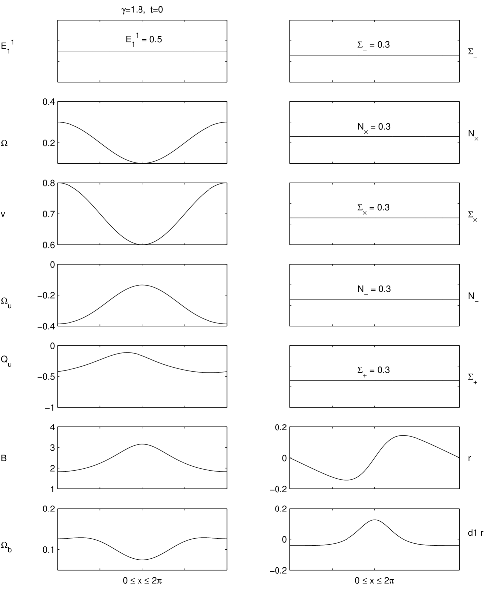
FIG. 1.: Isotropic singularity to the past for $\gamma>4/3$: $\gamma=1.8$, $t=0$

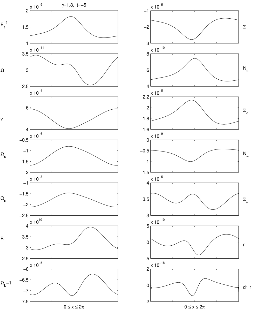
FIG. 2.: Isotropic singularity to the past for $\gamma>4/3$: $\gamma=1.8$, $t=-5$

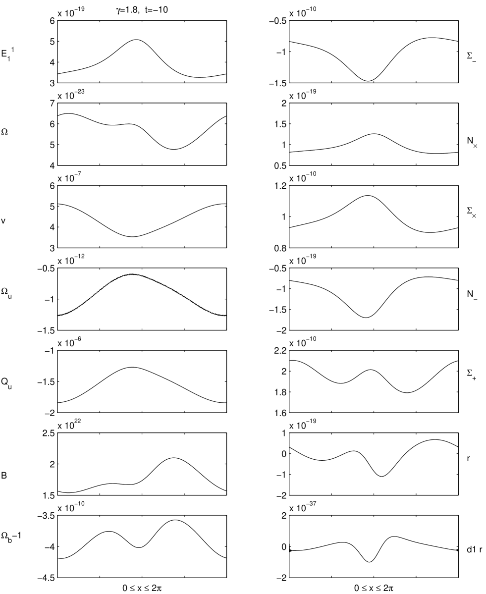
FIG. 3.: Isotropic singularity to the past for $\gamma>4/3$: $\gamma=1.8$, $t=-10$

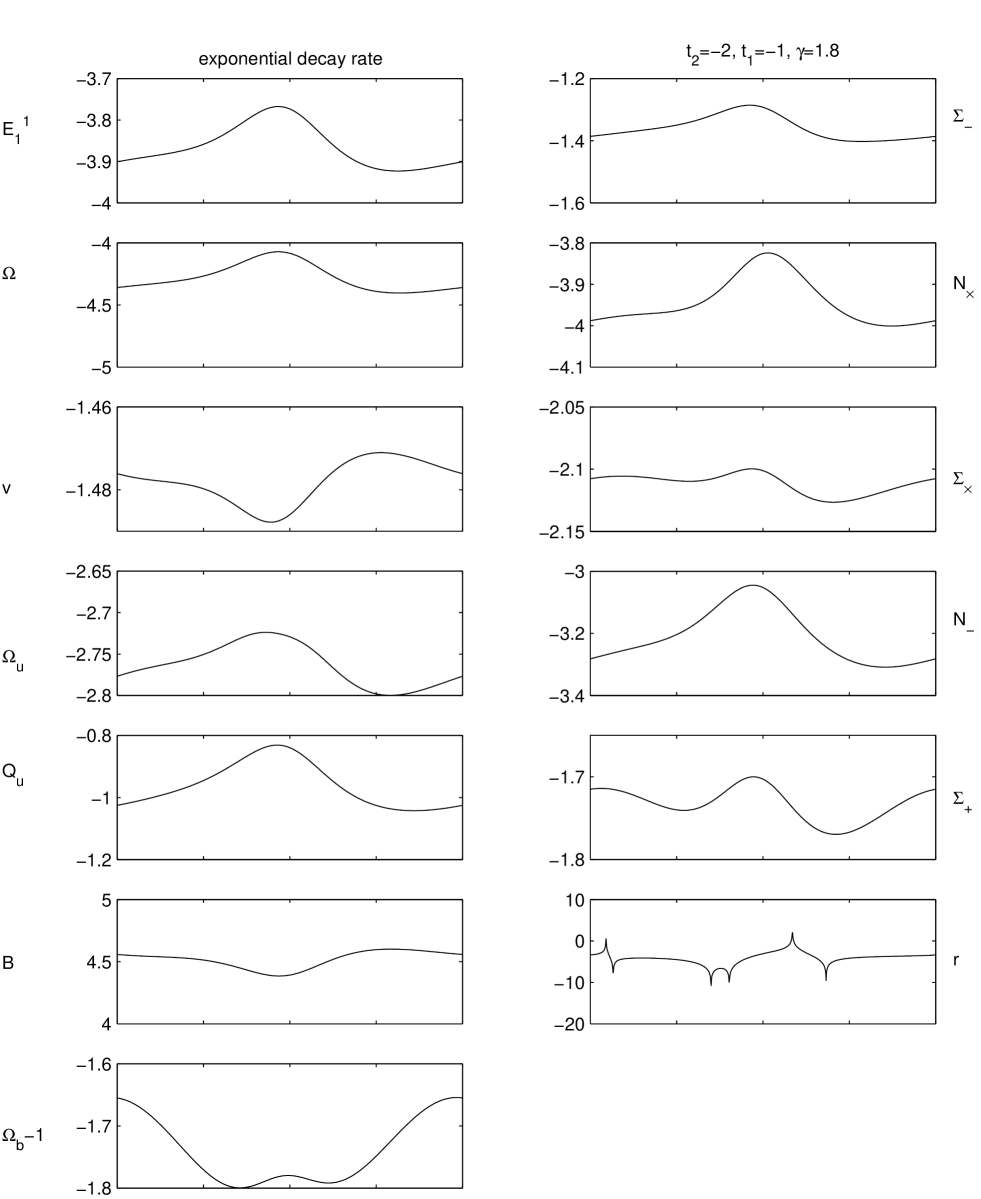
FIG. 4.: Exponential decay rates: $\gamma=1.8$, $t_{1}=-1$ and $t_{2}=-2$

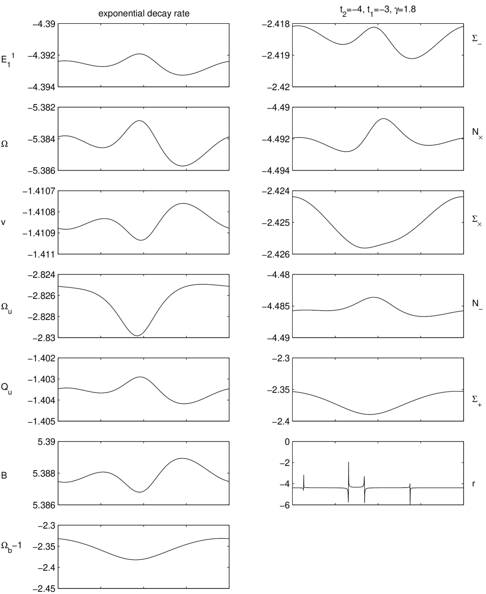
FIG. 5.: Exponential decay rates: $\gamma=1.8$, $t_{1}=-3$ and $t_{2}=-4$

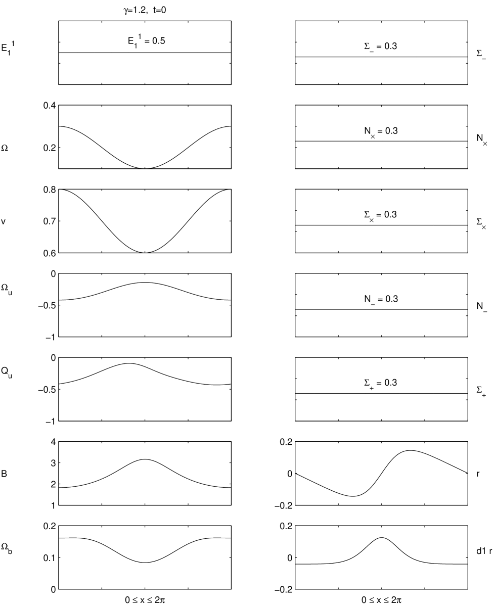
FIG. 6.: Initial singularity for $\gamma<4/3$: $\gamma=1.2$, $t=0$

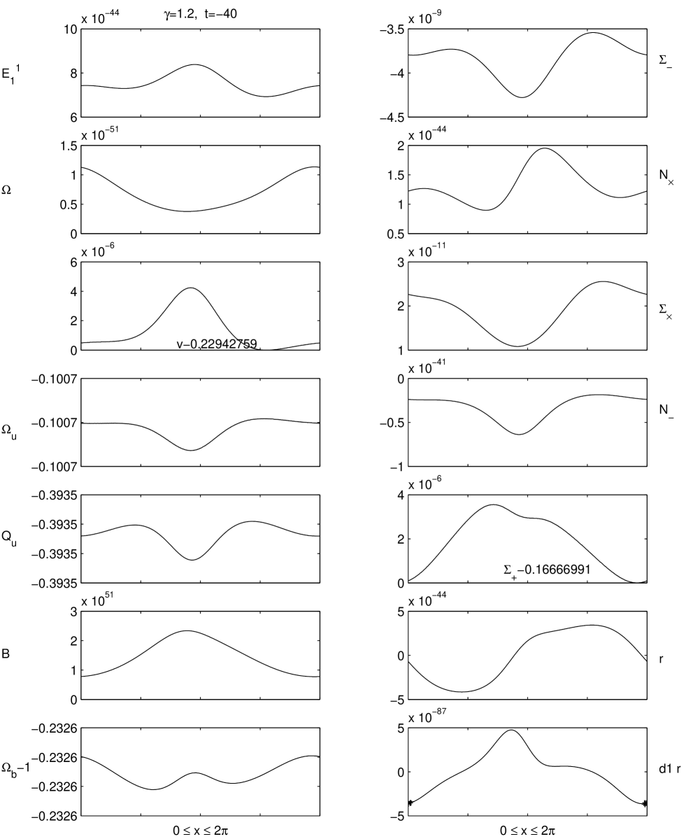
FIG. 7.: Initial singularity for $\gamma<4/3$: $\gamma=1.2$, $t=-40$

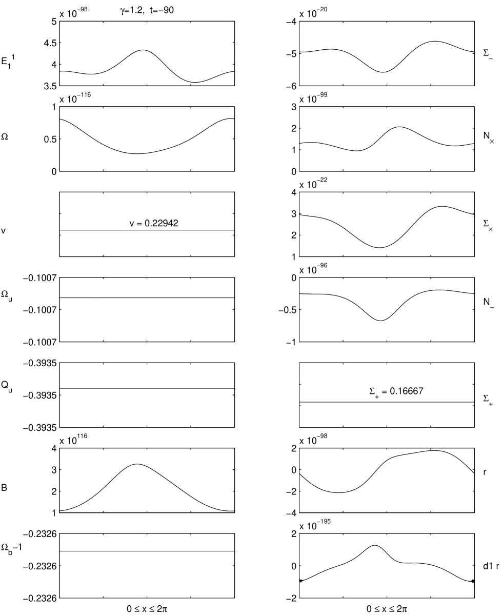
FIG. 8.: Initial singularity for $\gamma<4/3$: $\gamma=1.2$, $t=-90$

REFERENCES

[1]
V. Rubakov and M. E. Shaposhnikov, Phys. Lett. B125, 136
(1983); N. Arkani-Hamed, S. Dimopoulos, G. Dvali and N. Kaloper,
Phys. Rev. Lett. 84, 586 (2000).
[2]
L. Randall and R. Sundrum, Phys. Rev. Lett. 83, 3370 (1999); ibid83, 4690 (1999);
N. Arkani-Hamed, S. Dimopoulos, G. Dvali and N. Kaloper, Phys.
Rev. Lett. 84, 586 (2000); A. Chamblin and G. W. Gibbons, Phys. Rev.
Lett. 84, 1090 (2000).
[3] P. Horava and E.
Witten, Nucl. Phys. B460, 506 (1996).
[4] T. Shiromizu, K. Maeda, and M. Sasaki,
Phys. Rev. D 62, 024012 (2000);
M. Sasaki, T. Shiromizu, and K. Maeda, Phys. Rev. D 62,
024008 (2000);
R. Maartens, Phys. Rev. D 62, 084023 (2000).
[5]
R. Maartens, Phys. Rev. D 62, 084023 (2000).
[6]
P. Bintruy, C. Deffayet, and D. Langlois, Nucl.
Phys. B565, 269 (2000).
[8] S.W. Goode and J. Wainwright, Class. Quantum Grav. 2, 99
(1985). S.W. Goode, A.A. Coley and J. Wainwright, Class. Quantum Grav.
9, 445 (1992).
[9] J.D. Barrow and S. Hervik, Class. Quant. Grav. 19 155 (2002).
[10] A. Coley and S. Hervik, Class. Quant. Grav. 20 3061 (2003).
[11] A.A. Coley, Phys. Rev. D 66 023512 (2002).
[12] H. van Elst, C. Uggla and J, Wainwright, Class. Quantum Grav.
19, 51 (2002).
[13] D. Langlois, R. Maartens, M. Sasaki, and D. Wands, Phys. Rev. D, 63 084009 (2001).
[14]
B. K. Berger and V. Moncrief, Phys. Rev. D 48, 4676 (1993);
ibid , Phys. Rev. D 58, 064023 (1998); B. K. Berger
and D. Garfinkle, Phys. Rev. D 57, 4767 (1998).
[15]
M. Weaver, J. Isenberg and B. K. Berger, Phys. Rev. Letts. 80, 2984 (1998).
[16] J. Wainwright and G. F. R. Ellis (eds) Dynamical Systems in
Cosmology (Cambridge: Cambridge University Press, 1997).
[17]
M. A. H. MacCallum, Cosmological models from a geometric point of
view Cargèse Lectures in Physics Vol. 6 ed Schatzman E
(New York: Gordon and Breach) p 61 (1973)
[18]
H. van Elst and C. Uggla, Class. Quant. Grav. 14 2673 (1997).
[19] R. J. LeVeque Finite Volume Methods
for Hyperbolic Problems (Cambridge: Cambridge Univeristy Press, 2002).
[20] M. Bruni and P. Dunsby, Phys. Rev. D 66, 101301 (2002).
see also Dunsby et al., preprint.
[21] W. C. Lim, H. van Elst, C. Uggla and J. Wainwright, gr-qc/0306118.
[22] W. C. Lim, unpublished.
[23] C. G. Hewitt, R. Bridson and J. Wainwright,
Class. Quant. Grav. , gr-qc/0008037 (2000).
[24] V. G. LeBlanc, D. Kerr and J. Wainwright, Class. Quant. Grav. 20, 1757 (1995).
[25]
A.Campos and C. F. Sopuerta, Phys. Rev. D 63,
104012 (2001) and D 64, 104011 (2001).
R. J. van den Hoogen, A. A. Coley and Y. He, Phys. Rev. 68, 023502 (2003).
R. J. van den Hoogen and J. Ibanez, Phys. Rev. D 67,
083510 (2003).
[26] S. Mukohyama, private communication: see also Phys. Rev. D 62, 084015 (2000).
[27] K. Maeda, and T. Torii hep-th/0309152.
[28] J.D. Barrow, Nature 272 211 (1978).
[29]R. Penrose, in General relativity: An Einstein centenary survey, p 581
eds. S.W. Hawking and W. Israel (Cambridge University Press, 1979)
[30] D. S. Goldwirth and T. Piran, Phys. Rev. D 40, 3263 (1989).
D. S. Goldwirth, Phys. Lett. B 243, 41 (1990).
D. S. Goldwirth and T. Piran, Phys. Rep. 214, 223 (1993).
[31]
J. H. Kung and H. Brandenberger, Phys. Rev. D 42, 1008 (1990).
A. Albrecht, R. H. Brandenberger and R. Matzner, Phys. Rev. D 35, 429 (1987).
T. Chiba, T. Nakao and T. Nakamura, Phys. Rev. D 49, 3886 (1994).
O. Iguchi and H. Ishihara, Phys. Rev. D 56, 3216 (1997).
T. Vachaspati and M. Trodden, Phys. Rev. D 61, 023502 (1999).
[32]
R. Brandenberger, G. Geshnizjani and S. Watson. hep-th/ 0302222.