A family of filters to search for frequency dependent gravitational wave stochastic backgrounds

Abstract

We consider a three dimensional family of filters based on broken power-law spectra to search for gravitational wave stochastic backgrounds in the data from Earth-based laser interferometers. We show that such templates produce the necessary fitting factor for a wide class of cosmological backgrounds and astrophysical foregrounds and that the total number of filters required to search for those signals in the data from first generation laser interferometers operating at the design sensitivity is fairly small.

1 Introduction

Gravitational wave (GW) stochastic backgrounds represent one of the classes of signals that could be detected by Earth-based laser interferometers. Stringent upper-limits and/or detection will provide new insights into the evolution of the Universe at early cosmic times and high energy and, possibly, information about large populations of faint unresolved astrophysical sources at low-to-moderate redshift (see e.g. [1] and references therein for a recent review). The energy and spectral content of a stochastic background of gravitational waves are encoded in its spectrum $\Omega(f)\equiv(1/\rho_{\rm c})\,(d\rho(f)/d\ln f)$, where $\rho(f)$ is the energy density in GWs and $\rho_{\rm c}$ is the total energy density to close the Universe today. The current analysis of the data from Earth-based laser interferometers is restricted to stochastic signals whose spectrum is constant over the observational window, i.e. $\Omega(f)=$ const. However, some theoretical models suggest that a wide class of stochastic backgrounds are actually described by a frequency dependent spectrum, peaked at some characteristic frequency (that depends on the model parameters), with $\Omega(f)$ following roughly a ”broken power-law” behaviour; this is true both for cosmological backgrounds and astrophysical foregrounds (see for instance [2, 3]). In the near future it is therefore important to generalise the analysis of the data for this class of signals.

In this paper we evaluate whether the use of templates corresponding to a broken power-law spectrum $\Omega(f)$ is suitable to search for stochastic backgrounds characterised by a fairly general frequency dependent spectrum. In particular, for this class of templates we investigate the fitting factor and estimate the related computational costs.

2 Filter family and fitting factor

We consider a family of filters corresponding to a class of broken power-law spectra described by 3 parameters: a ”knee” frequency $f_{s}$ and two slopes $a$ and $b$. We choose the following functional form for the spectrum

$$\Omega_{\rm BPL}(f;{\mbox{\boldmath$\lambda$}}) = \Omega_{0}\,\left[A_{-}\left(\frac{f}{f_{s}}\right)^{a}+A_{+}\left(\frac{f}{f_{s}}\right)^{b}\right]\,,$$ (1)

where $\Omega_{0}$ is simply a normalisation factor and does not represent a search parameter and the functions $A_{\pm}$ are step functions.

The real signal will most unlikely match exactly the functional form (1), and we need to explore the Fitting Factor (FF) [4] of the template family (1). Lacking any solid prediction about the expected signals, we have computed the FF of broken power-law templates for a broad class of spectra $\Omega(f)$. We have considered a Gaussian-shaped spectrum, described by the two free parameters $f_{\rm G}$ and $\Delta f_{\rm G}$, a Lorenzian-shaped spectrum, described by the two free parameters $f_{\rm L}$ and $\Delta f_{\rm L}$, and a broken power-law spectrum modulated by an oscillatory term, whose free parameters are, beside $(a\,,b\,,f_{s})$, the amplitude $A_{\rm osc}$ and the frequency $f_{\rm osc}$. The corresponding spectra read

$$\Omega_{G}(f;{\mbox{\boldmath$\lambda$}}) = \Omega_{0}\,\exp\left[-\frac{(f-f_{\rm G})^{2}}{2(\Delta f_{\rm G})^{2}}\right]$$ (2)

$$\Omega_{L}(f;{\mbox{\boldmath$\lambda$}}) = \Omega_{0}\,\left[1+\frac{(f-f_{\rm L})^{2}}{(\Delta f_{\rm L})^{2}}\right]^{-1}$$ (3)

$$\Omega_{\rm osc}(f;{\mbox{\boldmath$\lambda$}}) = \Omega_{\rm BPL}(f;{\mbox{\boldmath$\lambda$}})\,\times\left[1+A_{\rm osc}\,\cos\left(2\pi\frac{f}{f_{\rm osc}}\right)\right]$$ (4)

The above functional forms $\Omega_{\rm G}(f)$, $\Omega_{\rm L}(f)$ and $\Omega_{\rm osc}(f)$ capture the behaviour of the spectra that characterise a wide class of cosmological and astrophysical models (see e.g. [2, 3]).

We have computed the fitting factor of the templates $\Omega_{\rm BPL}(f)$, Eq. (1), for $\Omega_{\rm G}(f)$, $\Omega_{\rm L}(f)$ and $\Omega_{\rm osc}(f)$. The results are summarised in Figure 1. It is clear that by suitably choosing the parameter space for the slopes $a$ and $b$ one can detect essentially any spectrum characterised by a Gaussian/Lorenzian shape. Even if the real signal shows fairly strong and rapid oscillations superimposed to the general power-law behaviour, the templates $\Omega_{\rm BPL}(f)$ can still have a fitting factor greater than $0.97\%$, except in extreme cases. The main outcome of this analysis is therefore that power-law templates are indeed suitable for searching for fairly general frequency dependent stochastic backgrounds.

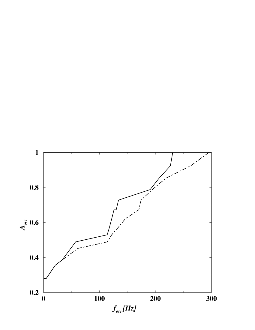
Figure 1: The fitting factor of “broken power-law” template families. Left: The plot shows, as a function of $|a_{\rm max}|=|b_{\rm max}|$, the minimum value of $\Delta f_{\rm G}$ (solid line top) and $\Delta f_{\rm L}$ (dotted-line bottom) corresponding to $FF>0.97$ for backgrounds characterised by a spectrum  (2) and (3), respectively.
Right: The plot shows, as a function of $f_{\rm osc}$, the maximum amplitude $A_{\rm osc}$ for a signal (4) for which $FF>0.97$ over a frequency band $40$Hz-$1$kHz. The two curves correspond to a knee frequency $f_{s}$ in the signal corresponding to 100 Hz (top) and 1kHz (bottom), respectively. The slopes for both $\Omega_{\rm BPL}(f)$ and $\Omega_{\rm osc}$ are $a=2$ and $b=-2$.

3 Number of filters

We can now address the computational requirements to set up a search using the templates $\Omega_{\rm BPL}(f)$. In order to compute the total number of filters we have extended the geometrical formalism developed in  [6] to the case of stochastic backgrounds. The basic idea is the following: the signal is a vector in the vector space of the data and the $N$-parameter family of templates traces out an $N$-dimensional template manifold. The parameters themselves are coordinates on this manifold, and one can introduce a $N\times N$ non-flat metric $\gamma_{jk}$ which is related to the fractional loss in the signal-to-noise ratio when there is a mismatch of parameters between the signal and the filter. The spacing of the grid of filters is determined by the fractional loss due to the maximum tolerable mismatch $\mu$, which fixes the grid spacing of the filters in the parameter space $\cal P$. For a a hyper-rectangular mesh (which does not represent necessarily the most efficient tiling of the parameter space) the number of filters ${\cal N}$ is given by

$${\cal N}=\left[\frac{1}{2}\sqrt{N\over\mu}\right]^{N}\,\int_{{\cal P}}d^{N}{\lambda}\sqrt{\det||\gamma_{jk}||}\,;$$ (5)

In particular, by adopting a detection strategy based upon the cross correlation statistics [5], for a stochastic signal characterised by the spectrum  (1) the metric $\gamma_{jk}$ is represented by a $3\times 3$ symmetric matrix whose components depend on the following inner product (involving the optimal filter $Q$) and its $1^{st}$ and $2^{nd}$ derivatives with respect to the slopes $(a,b)$ and to the “knee” frequency $f_{s}$ (a more detailed derivation can be found in [7])

$$\left<Q,Q\right>=\int_{f_{min}}^{f_{max}}df\,\frac{\gamma^{2}(f)\Omega^{2}_{\rm BPL}(f;{\mbox{\boldmath$\lambda$}})}{f^{6}\,S_{1}(f)\,S_{2}(f)}$$ (6)

where $(f_{min},f_{max})$ are the low-frequency and high-frequency cut-off of the interferometer band (chosen to be $40$Hz and $1$kHz respectively), $S_{1,2}$ are the noise spectral densities of the detectors and $\gamma$ is the overlap reduction function.

We have applied this formalism to stochastic backgrounds whose spectrum is given by (1) and we have computed ${\cal N}$ for $N=3$ and $\mu=0.03$ (a $3\%$ maximum tolerable mismatch) for the case of cross-correlations between the Livingston and Hanford LIGO interferometers operating at the designed sensitivity over $10^{7}$ sec of integration time. Figure 2 summarises the results. In particular, we have considered both the more likely case of broken power law spectra with a peak in the sensitive region of the detector frequency band - e.g. due to a phase transition in the Early Universe -(dash-dot line) and the case when also spectra with a “valley” are taken into account (solid line). It is clear that for a 3-dimensional search over the parameter space $40\,{\rm Hz}\leq f_{s}\leq 1\,{\rm kHz}$ and $-10\leq a,b\leq 10$ - which essentially covers the relevant parameter space (see previous section)- the total number of filters that are required for a 3% mismatch is $\lower 2.15277pt\hbox{$\;\buildrel<\over{\sim}\;$}500$. This represents a modest number of filters, and the search does not pose any significant challenge as far as computational time is concerned.

Figure 2: The number of filters for a search based on “broken power-law” templates. Left: The plot shows the total number of filters, assuming to know a priori the frequency $f_{s}$, required to carry out the analysis over $10^{7}$ sec by cross-correlating the data streams from the two LIGO interferometers at designed sensitivity, as a function of $f_{s}$. The range of the slopes is $-10\leq a,b\leq 10$. Notice that, as expected, the largest number of filters corresponds to $f_{s}$ right at the heart of the sensitivity window. Right: The plot shows the total number of filters for the general case of a $3-$dimensional parameter search (both on the spectral slopes and the knee frequency). We show the total number of filters as a function of the maximum value ($a_{\rm max}$) of the slope parameter $a$, assuming a maximum signal-to-noise ratio loss of $3\%$, for two different choices of the parameter space: (i) $a_{\rm min}=b_{\rm min}=-10$, $b_{\rm max}=a_{\rm max}$ (solid line), and (ii) $a_{\rm min}=b_{\rm max}=0$, $b_{\rm min}=-a_{\rm max}$ (dashed-dotted line).

4 Conclusions

We have considered a family of templates characterised by a broken power-law spectrum to search for fairly general classes of frequency-dependent gravitational wave stochastic backgrounds. We have shown that templates corresponding to broken-power law spectra have the necessary fitting-factor (i.e. greater than $97\%$) for a wide class of models and that the total number of filters required to carry out a search using the data from first generation laser interferometer is sufficiently small not to produce a large computational burden.

References

References

- [1] Maggiore M (2000) Phys. Rept. 331 283
- [2] Buonanno A, Maggiore M. and Ungarelli C. (1997) Phys. Rev. D 55 3330.
- [3] Farmer A.J. and Phinney E.S. (2003) astro-ph/0304393.
- [4] Apostolatos T.A. (1995) Phys. Rev. D 52 605.
- [5] Allen B and Romano J.D. (1999) Phys. Rev. D 59 102001
- [6] Owen B (1996) Phys.Rev. D 53 6749
- [7] Ungarelli C and Vecchio A, in preparation.