BRANE-WORLD GRAVITY

Abstract

The observable universe could be a 1+3-surface (the “brane”) embedded in a 1+3+$d$-dimensional spacetime (the “bulk”), with Standard Model particles and fields trapped on the brane while gravity is free to access the bulk. At least one of the $d$ extra spatial dimensions could be very large relative to the Planck scale, which lowers the fundamental gravity scale, possibly even down to the electroweak ($\sim$TeV) level. This revolutionary picture arises in the framework of recent developments in M theory. The 1+10-dimensional M theory encompasses the known 1+9-dimensional superstring theories, and is widely considered to be a promising potential route to quantum gravity. General relativity cannot describe gravity at high enough energies and must be replaced by a quantum gravity theory, picking up significant corrections as the fundamental energy scale is approached. At low energies, gravity is localized at the brane and general relativity is recovered, but at high energies gravity “leaks” into the bulk, behaving in a truly higher-dimensional way. This introduces significant changes to gravitational dynamics and perturbations, with interesting and potentially testable implications for high-energy astrophysics, black holes and cosmology. Brane-world models offer a phenomenological way to test some of the novel predictions and corrections to general relativity that are implied by M theory. This review discusses the geometry, dynamics and perturbations of simple brane-world models for cosmology and astrophysics, mainly focusing on warped 5-dimensional brane-worlds based on the Randall-Sundrum models.

I Introduction

At high enough energies, Einstein’s theory of general relativity breaks down, and will be superceded by a quantum gravity theory. The classical singularities predicted by general relativity in gravitational collapse and in the hot big bang will be removed by quantum gravity. But even below the fundamental energy scale that marks the transition to quantum gravity, significant corrections to general relativity will arise. These corrections could have a major impact on the behaviour of gravitational collapse, black holes and the early universe, and they could leave a trace–a “smoking gun”–in various observations and experiments. Thus it is important to estimate these corrections and develop tests for detecting them or ruling them out. In this way, quantum gravity can begin to be subject to testing by astrophysical and cosmological observations.

Developing a quantum theory of gravity and a unified theory of all the forces and particles of nature are the two main goals of current work in fundamental physics. There is as yet no generally accepted (pre-)quantum gravity theory. Two of the main contenders are M theory mtheory and quantum geometry (loop quantum gravity) loop . It is important to explore the astrophysical and cosmological predictions of both these approaches. This review considers only models that arise within the framework of M theory, and mainly the 5-dimensional warped brane-worlds.

I.1 Heuristics of higher-dimensional gravity

One of the fundamental aspects of string theory is the need for extra spatial dimensions. This revives the original higher-dimensional ideas of Kaluza and Klein in the 1920’s, but in a new context of quantum gravity. An important consequence of extra dimensions is that the 4-dimensional Planck scale $M_{\rm p}\equiv M_{4}$ is no longer the fundamental scale, which is $M_{4+d}$, where $d$ is the number of extra dimensions. This can be seen from the modification of the gravitational potential. For an Einstein-Hilbert gravitational action we have,

$$S_{\rm gravity}={1\over 2\kappa_{4+d}^{2}}\int{\rm d}^{4}x\,{\rm d}^{d}y\,\sqrt{-^{(4+d)\!}g}\left[\,{}^{(4+d)\!}R-2\Lambda_{4+d}\right]\,,$$ (1)

$${}^{(4+d)\!}G_{AB}\equiv^{(4+d)\!}R_{AB}-{1\over 2}\,^{(4+d)\!}R\,\,^{(4+d)\!}g_{AB}=-\Lambda_{4+d}{}^{(4+d)\!}g_{AB}+\kappa_{4+d}^{2}\,\,{}^{(4+d)\!}T_{AB}\,,$$ (2)

where $X^{A}=(x^{\mu},y^{1},\cdots,y^{d})$ and $\kappa_{4+d}^{2}$ is the gravitational coupling constant,

$$\kappa_{4+d}^{2}=8\pi G_{4+d}={8\pi\over M_{4+d}^{2+d}}\,.$$ (3)

The static weak field limit of the field equations leads to the $4+d$-dimensional Poisson equation, whose solution is the gravitational potential,

$$V(r)\propto{\kappa_{4+d}^{2}\over r^{1+d}}\,.$$ (4)

If the length scale of the extra dimensions is $L$, then on scales $r\lesssim L$, the potential is $4+d$-dimensional, $V\sim r^{-(1+d)}$. By contrast, on scales large relative to $L$, where the extra dimensions do not contribute to variations in the potential, $V$ behaves like a 4-dimensional potential, i.e., $r\sim L$ in the $d$ extra dimensions, and $V\sim L^{-d}r^{-1}$. This means that the usual Planck scale becomes an effective coupling constant, describing gravity on scales much larger than the extra dimensions, and related to the fundamental scale via the volume of the extra dimensions:

$$M_{\rm p}^{2}\sim M_{4+d}^{2+d}\,L^{d}\,.$$ (5)

If the extra-dimensional volume is Planck scale, i.e. $L\sim M_{\rm p}^{-1}$, then $M_{4+d}\sim M_{\rm p}$. But if the extra-dimensional volume is significantly above Planck-scale, then the true fundamental scale $M_{4+d}$ can be much less than the effective scale $M_{\rm p}\sim 10^{19}~{}{\rm GeV}$. In this case, we understand the weakness of gravity as due to the fact that it “spreads” into extra dimensions and only a part of it is felt in 4 dimensions.

A lower limit on $M_{4+d}$ is given by null results in table-top experiments to test for deviations from Newton’s law in 4 dimensions, $V\propto r^{-1}$. These experiments currently exp probe sub-millimetre scales, so that

$$L\lesssim 10^{-1}~{}{\rm mm}\sim(10^{-15}~{}{\rm TeV})^{-1}~{}\Rightarrow~{}M_{4+d}\gtrsim 10^{(32-15d)/(d+2)}~{}{\rm TeV}\,.$$ (6)

Stronger bounds for brane-worlds with compact flat extra dimensions can be derived from null results in particle accelerators and in high-energy astrophysics cav ; cheung ; hanraf .

I.2 Brane-worlds and M theory

String theory thus incorporates the possibility that the fundamental scale is much less than the Planck scale felt in 4 dimensions. There are five distinct 1+9-dimensional superstring theories, all giving quantum theories of gravity. Discoveries in the mid-90 s of duality transformations that relate these superstring theories and the 1+10-dimensional supergravity theory, led to the conjecture that all of these theories arise as different limits of a single theory, which has come to be known as M theory. The 11th dimension in M theory is related to the string coupling strength; the size of this dimension grows as the coupling becomes strong. At low energies, M theory can be approximated by 1+10-dimensional supergravity.

It was also discovered that p-branes, which are extended objects of higher dimension than strings (1-branes), play a fundamental role in the theory. In the weak coupling limit, p-branes ($p>1$) become infinitely heavy, so that they do not appear in the perturbative theory. Of particular importance among p-branes are the D-branes, on which open strings can end. Roughly speaking, open strings, which describe the non-gravitational sector, are attached at their endpoints to branes, while the closed strings of the gravitational sector can move freely in the bulk. Classically, this is realised via the localization of matter and radiation fields on the brane, with gravity propagating in the bulk (see Fig. 1).

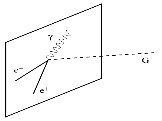
Figure 1: Schematic of confinement of matter to the brane, while gravity propagates in the bulk (from cav ).

In the Horava-Witten solution hv , gauge fields of the standard model are confined on two 1+9-branes located at the end points of an $S^{1}/Z_{2}$ orbifold, i.e., a circle folded on itself across a diameter. The 6 extra dimensions on the branes are compactified on a very small scale, close to the fundamental scale, and their effect on the dynamics is felt through “moduli” fields, i.e. 5D scalar fields. A 5D realization of the Horava-Witten theory and the corresponding brane-world cosmology is given in low .

These solutions can be thought of as effectively 5-dimensional, with an extra dimension that can be large relative to the fundamental scale. They provide the basis for the Randall-Sundrum 2-brane models of 5-dimensional gravity rs1 (see Fig. 2). The single-brane Randall-Sundrum models rs2 with infinite extra dimension arise when the orbifold radius tends to infinity. The RS models are not the only phenomenological realizations of M theory ideas. They were preceded by the Arkani-Hamed-Dimopoulos-Dvali (ADD) add brane-world models, which put forward the idea that a large volume for the compact extra dimensions would lower the fundamental Planck scale,

$$M_{\rm ew}\sim 1~{}{\rm TeV}\,\lesssim M_{4+d}\leq M_{\rm p}\sim 10^{16}~{}{\rm TeV}\,,$$ (7)

where $M_{\rm ew}$ is the electroweak scale. If $M_{4+d}$ is close to the lower limit in Eq. (7), then this would address the long-standing “hierarchy” problem, i.e. why there is such a large gap between $M_{\rm ew}$ and $M_{\rm p}$.

In the ADD models, more than one extra dimension is required for agreement with experiments, and there is “democracy” amongst the equivalent extra dimensions, which are typically flat. By contrast, the RS models have a “preferred” extra dimension, with other extra dimensions treated as ignorable (i.e., stabilized except at energies near the fundamental scale). Furthermore, this extra dimension is curved or “warped” rather than flat: the bulk is a portion of anti de Sitter (AdS₅) spacetime. As in the Horava-Witten solutions, the RS branes are $Z_{2}$-symmetric (mirror symmetry), and have a tension, which serves to counter the influence of the negative bulk cosmological constant on the brane. This also means that the self-gravity of the branes is incorporated in the RS models. The novel feature of the RS models compared to previous higher-dimensional models is that the observable 3 dimensions are protected from the large extra dimension (at low energies) by curvature rather than straightforward compactification.

The RS brane-worlds and their generalizations (to include matter on the brane, scalar fields in the bulk, etc.) provide phenomenological models that reflect at least some of the features of M theory, and that bring exciting new geometric and particle physics ideas into play. The RS2 models also provide a framework for exploring holographic ideas that have emerged in M theory. Roughly speaking, holography suggests that higher-dimensional gravitational dynamics may be determined from knowledge of the fields on a lower-dimensional boundary. The AdS/CFT correspondence is an example, in which the classical dynamics of the higher-dimensional gravitational field are equivalent to the quantum dynamics of a conformal field theory (CFT) on the boundary. The RS2 model with its AdS₅ metric satisfies this correspondence to lowest perturbative order acft (see also acftcosmo for the AdS/CFT correspondence in a cosmological context).

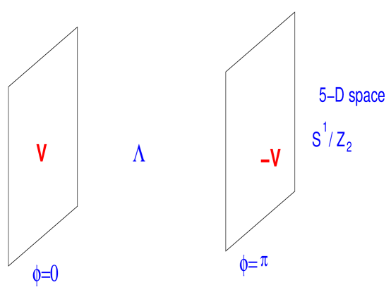
Figure 2: The RS 2-brane model (from cheung ).

In this review, I focus on RS brane-worlds (mainly RS 1-brane) and their generalizations, with the emphasis on geometry and gravitational dynamics (see m2 ; rev ; lan for previous reviews with a broadly similar approach). Other recent reviews focus on string-theory aspects, e.g. que , or on particle physics aspects, e.g. r ; cav . Before turning to a more detailed analysis of RS brane-worlds, I discuss the notion of Kaluza-Klein (KK) modes of the graviton.

I.3 Heuristics of KK modes

The dilution of gravity via extra dimensions not only weakens gravity on the brane, it also extends the range of graviton modes felt on the brane beyond the massless mode of 4-dimensional gravity. For simplicity, consider a flat brane with one flat extra dimension, compactified through the identification $y\leftrightarrow y+2\pi nL$, where $n=0,1,2,\cdots$. The perturbative 5D graviton amplitude can be Fourier expanded as

$$f(x^{a},y)=\sum_{n}e^{iny/L}\,f_{n}(x^{a})\,,$$ (8)

where $f_{n}$ are the amplitudes of the KK modes, i.e. the effective 4D modes of the the 5D graviton. To see that these KK modes are massive from the brane viewpoint, we start from the 5D wave equation that the massless 5D field $f$ satisfies (in a suitable gauge):

$${}^{(5)}\!\Box f=0~{}\Rightarrow~{}\Box f+\partial_{y}^{2}f=0\,.$$ (9)

It follows that the KK modes satisfy a 4D Klein-Gordon equation with an effective 4D mass, $m_{n}$,

$$\Box f_{n}=m_{n}^{2}\,f_{n}\,,~{}~{}m_{n}={n\over L}\,.$$ (10)

The massless mode, $f_{0}$, is the usual 4D graviton mode. But there is a tower of massive modes, $L^{-1},2L^{-1},\cdots$, which imprint the effect of the 5D gravitational field on the 4D brane. Compactness of the extra dimension leads to discreteness of the spectrum. For an infinite extra dimension, $L\to\infty$, the separation between the modes disappears and the tower forms a continuous spectrum. In this case, the coupling of the KK modes to matter must be very weak in order to avoid exciting the lightest massive modes with $m\gtrsim 0$.

From a geometric viewpoint, the KK modes can also be understood via the fact that the projection of the null graviton 5-momentum ${}^{(5)}\!p_{A}$ onto the brane is timelike. If the unit normal to the brane is $n_{A}$, then the induced metric on the brane is

$$g_{AB}=\,^{(5)}\!g_{AB}-n_{A}n_{B}\,,~{}^{(5)}\!g_{AB}n^{A}n^{B}=1\,,~{}g_{AB}n^{B}=0\,,$$ (11)

and the 5-momentum may be decomposed as

$${}^{(5)}\!p_{A}=mn_{A}+p_{A}\,,~{}p_{A}n^{A}=0\,,~{}m=\,^{(5)}\!p_{A}\,n^{A}\,,$$ (12)

where $p_{A}=g_{AB}\,^{(5)}\!p^{B}$ is the projection along the brane, depending on the orientation of the 5-momentum relative to the brane. The effective 4-momentum of the 5D graviton is thus $p_{A}$. Expanding ${}^{(5)}\!g_{AB}{}\,{}^{(5)}\!p^{A}\,{}^{(5)}\!p^{B}=0$, we find that

$$g_{AB}p^{A}p^{B}=-m^{2}\,.$$ (13)

It follows that the 5D graviton has an effective mass $m$ on the brane. The usual 4D graviton corresponds to the zero mode, $m=0$, when ${}^{(5)}\!p_{A}$ is tangent to the brane.

The extra dimensions lead to new scalar and vector degrees of freedom on the brane. In 5D, the spin-2 graviton is represented by a metric perturbation ${}^{(5)}\!h_{AB}$ that is transverse traceless:

$${}^{(5)}\!h^{A}{}_{A}=0=\partial_{B}\,^{(5)}\!h_{A}{}^{B}\,.$$ (14)

In a suitable gauge, ${}^{(5)}\!h_{AB}$ contains a 3D transverse traceless perturbation $h_{ij}$, a 3D transverse vector perturbation $\Sigma_{i}$ and a scalar perturbation $\beta$, which each satisfy the 5D wave equation durkoc :

$${}^{(5)}\!h_{AB}~{}\longrightarrow~{}h_{ij}\,,~{}\Sigma_{i}\,,~{}\beta\,,$$ (15)

$$h^{i}{}_{i}=0=\partial_{j}h^{ij}\,,~{}\partial_{i}\Sigma^{i}=0\,,$$ (16)

$$(\Box+\partial_{y}^{2})\left(\begin{array}[]{c}\beta\\ \Sigma_{i}\\ h_{ij}\end{array}\right)=0\,.$$ (20)

The other components of ${}^{(5)}\!h_{AB}$ are determined via constraints once these wave equations are solved. The 5 degrees of freedom (polarizations) in the 5D graviton are thus split into 2 ($h_{ij}$) + 2 ($\Sigma_{i}$) +1 ($\beta$) degrees of freedom in 4D. On the brane, the 5D graviton field is felt as

• a 4D spin-2 graviton $h_{ij}$ (2 polarizations)

• a 4D spin-1 gravi-vector (gravi-photon) $\Sigma_{i}$ (2 polarizations)

• a 4D spin-0 gravi-scalar $\beta$.

The massive modes of the 5D graviton are represented via massive modes in all 3 of these fields on the brane. The standard 4D graviton corresponds to the massless zero-mode of $h_{ij}$.

In the general case of $d$ extra dimensions, the number of degrees of freedom in the graviton follows from the irreducible tensor representations of the isometry group as ${1\over 2}(d+1)(d+4)$.

II Randall-Sundrum brane-worlds

RS brane-worlds do not rely on compactification to localize gravity at the brane, but on the curvature of the bulk (sometimes called “warped compactification”). What prevents gravity from ‘leaking’ into the extra dimension at low energies is a negative bulk cosmological constant,

$$\Lambda_{5}=-{6\over\ell^{2}}=-6\mu^{2},$$ (21)

where $\ell$ is the curvature radius of AdS₅ and $\mu$ is the corresponding energy scale. The curvature radius determines the magnitude of the Riemann tensor:

$${}^{(5)}\!R_{ABCD}=-{1\over\ell^{2}}\left[\,{}^{(5)}\!g_{AC}\,^{(5)}\!g_{BD}-\,^{(5)}\!g_{AD}\,^{(5)}\!g_{BC}\right].$$ (22)

The bulk cosmological constant acts to “squeeze” the gravitational field closer to the brane. We can see this clearly in Gaussian normal coordinates $X^{A}=(x^{\mu},y)$ based on the brane at $y=0$, for which the AdS₅ metric takes the form

$${}^{(5)}\!ds^{2}=e^{-2|y|/\ell}\eta_{\mu\nu}dx^{\mu}dx^{\nu}+dy^{2}\,,$$ (23)

with $\eta_{\mu\nu}$ the Minkowski metric. The exponential warp factor reflects the confining role of the bulk cosmological constant. The $Z_{2}$-symmetry about the brane at $y=0$ is incorporated via the $|y|$ term. In the bulk, this metric is a solution of the 5D Einstein equations,

$$^{(5)}\!G_{AB}=-\Lambda_{5}\,\,^{(5)}\!g_{AB}\,,$$ (24)

i.e., ${}^{(5)}\!T_{AB}=0$ in Eq. (2). The brane is a flat Minkowski spacetime, $g_{AB}(x^{\alpha},0)=\eta_{\mu\nu}\delta^{\mu}{}_{A}\delta^{\nu}{}_{B}$, with self-gravity in the form of brane tension. One can also use Poincare coordinates, which bring the metric into manifestly conformally flat form:

$$^{(5)}\!ds^{2}={\ell^{2}\over z^{2}}\left[\eta_{\mu\nu}dx^{\mu}dx^{\nu}+dz^{2}\right]\,,$$ (25)

where $z=\ell e^{y/\ell}$.

The two RS models are distinguished as follows:

• RS 2-BRANE:

  There are two branes in this model rs1 , at $y=0$ and $y=L$, with $Z_{2}$-symmetry identifications

  $$y\leftrightarrow-y\,,~{}~{}y+L\leftrightarrow L-y\,.$$ (26)

  The branes have equal and opposite tensions, $\pm\lambda$, where

  $$\lambda={3M_{\rm p}^{2}\over 4\pi\ell^{2}}\,.$$ (27)

  The positive-tension brane has fundamental scale $M_{5}$ and is “hidden”. Standard model fields are confined on the negative tension (or “visible”) brane. Because of the exponential warping factor, the effective scale on the visible brane at $y=L$ is $M_{\rm p}$, where

  $$M_{\rm p}^{2}=M_{5}^{3}\,\ell\left[1-e^{-2L/\ell}\right]\,.$$ (28)

  So the RS 2-brane model gives a new approach to the hierarchy problem. Because of the finite separation between the branes, the KK spectrum is discrete. Furthermore, at low energies gravity on the branes becomes Brans-Dicke-like, with the sign of the Brans-Dicke parameter equal to the sign of the brane tension gt . In order to recover 4D general relativity at low energies, a mechanism is required to stabilize the inter-brane distance, which corresponds to a scalar field degree of freedom known as the radion goldwise ; 2b .

• RS 1-BRANE:

  In this model rs2 , there is only one, positive tension, brane. It may be thought of as arising from sending the negative tension brane off to infinity, $L\to\infty$. Then the energy scales are related via

  $$M_{5}^{3}={M_{\rm p}^{2}\over\ell}\,.$$ (29)

  The infinite extra dimension makes a finite contribution to the 5D volume because of the warp factor:

  $$\int\,d^{5}X\sqrt{-\,^{(5)}\!g}=2\int\,d^{4}x\,\int_{0}^{\infty}\,dye^{-4y/\ell}={\ell\over 2}\,\int\,d^{4}x\,.$$ (30)

  Thus the effective size of the extra dimension probed by the 5D graviton is $\ell$.

I will concentrate mainly on RS 1-brane from now on, referring to RS 2-brane occasionally. The RS 1-brane models are in some sense the most simple and geometrically appealing form of brane-world model, while at the same time providing a framework for the AdS/CFT correspondence acft ; acftcosmo . The RS 2-brane models introduce the added complication of radion stabilization, as well as possible complications arising from negative tension. However, they remain important and will occasionally be discussed.

In RS 1-brane, the negative $\Lambda_{5}$ is offset by the positive brane tension $\lambda$. The fine-tuning in Eq. (27) ensures that there is zero effective cosmological constant on the brane, so that the brane has the induced geometry of Minkowski spacetime. To see how gravity is localized at low energies, we consider the 5D graviton perturbations of the metric rs2 ; gt ; morepert :

$${}^{(5)}\!g_{AB}\to\,^{(5)}\!g_{AB}+e^{-2|y|/\ell}\,{}^{(5)}\!h_{AB}\,,~\,{}^{(5)}\!h_{Ay}=0=\,^{(5)}\!h^{\mu}{}_{\mu}=\,^{(5)}\!h^{\mu\nu}{}{}_{,\nu}\,.$$ (31)

(See Fig. 3.) This is the RS gauge, which is different from the gauge used in Eq. (15), but which also has no remaining gauge freedom. The 5 polarizations of the 5D graviton are contained in the 5 independent components of ${}^{(5)}\!h_{\mu\nu}$ in the RS gauge.

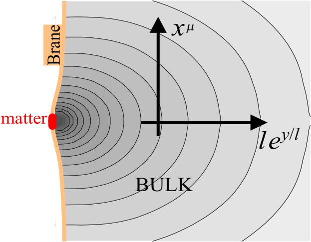
Figure 3: Gravitational field of small point particle on the brane in RS gauge (from gt ).

We split the amplitude $f$ of ${}^{(5)}\!h_{AB}$ into 3D Fourier modes, and the linearized 5D Einstein equations lead to the wave equation ($y>0$)

$$\ddot{f}+k^{2}f=e^{-2y/\ell}\left[f^{\prime\prime}-{4\over\ell}\,f^{\prime}\right]\,.$$ (32)

Separability means we can write

$$f(t,y)=\sum_{m}\varphi_{m}(t)\,f_{m}(y)\,,$$ (33)

and the wave equation reduces to

$$\ddot{\varphi}_{m}+(m^{2}+k^{2})\varphi_{m} = 0\,,$$ (34)

$$f_{m}^{\prime\prime}-{4\over\ell}\,f_{m}^{\prime}+e^{2y/\ell}m^{2}f_{m} = 0\,.$$ (35)

The zero mode solution is

$$\varphi_{0}(t) = A_{0+}e^{+ikt}+A_{0-}e^{-ikt}\,,$$ (36)

$$f_{0}(y) = B_{0}+C_{0}e^{4y/\ell}\,,$$ (37)

and the $m>0$ solutions are

$$\varphi_{m}(t) = A_{m+}\exp\left(+i\sqrt{m^{2}+k^{2}}\,t\right)+A_{m-}\exp\left(-i\sqrt{m^{2}+k^{2}}\,t\right)\,,$$ (38)

$$f_{m}(y) = e^{2y/\ell}\left[B_{m}J_{2}\left(m\ell e^{y/\ell}\right)+C_{m}Y_{2}\left(m\ell e^{y/\ell}\right)\right]\,.$$ (39)

The boundary condition for the perturbations arises from the junction conditions, Eq. (64), discussed below, and leads to $f^{\prime}(t,0)=0$, since the transverse traceless part of the perturbed energy-momentum tensor on the brane vanishes. This implies

$$C_{0}=0\,,~{}~{}C_{m}=-{J_{1}(m\ell)\over Y_{1}(m\ell)}\,B_{m}\,.$$ (40)

The zero mode is normalizable, since

$$\left|\int_{0}^{\infty}B_{0}e^{-2y/\ell}dy\right|<\infty\,.$$ (41)

Its contribution to the gravitational potential $V={1\over 2}\,^{(5)}\!h_{00}$ gives the 4D result, $V\propto r^{-1}$. The contribution of the massive KK modes sums to a correction of the 4D potential. For $r\ll\ell$, one obtains

$$V(r)\approx{GM\ell\over r^{2}}\,,$$ (42)

which simply reflects the fact that the potential becomes truly 5D on small scales. For $r\gg\ell$,

$$V(r)\approx{GM\over r}\left(1+{2\ell^{2}\over 3r^{2}}\right)\,,$$ (43)

which gives the small correction to 4D gravity at low energies from extra-dimensional effects. These effects serve to slightly strengthen the gravitational field, as expected.

Table-top tests of Newton’s laws currently find no deviations down to $O(10^{-1}~{}{\rm mm})$, so that $\ell\lesssim 0.1~{}$mm in Eq. (43). Then by Eqs. (27) and (29), this leads to lower limits on the brane tension and the fundamental scale of the RS 1-brane model:

$$\lambda>(1~{}{\rm TeV})^{4}\,,~{}M_{5}>10^{5}~{}{\rm TeV}\,.$$ (44)

These limits do not apply to the 2-brane case.

For the 1-brane model, the boundary condition, Eq. (40), admits a continuous spectrum $m>0$ of KK modes. In the 2-brane model, $f^{\prime}(t,L)=0$ must hold in addition to Eq. (40). This leads to conditions on $m$, so that the KK spectrum is discrete:

$$m_{n}={x_{n}\over\ell}\,e^{-L/\ell}\mbox{ where }Y_{1}(m\ell)J_{1}(x_{n})=J_{1}(m\ell)Y_{1}(x_{n})\,.$$ (45)

The limit Eq. (44) indicates that there are no observable collider, i.e. $O({\rm TeV})$, signatures for the RS 1-brane model. The 2-brane model by contrast, for suitable choice of $L$ and $\ell$ so that $m_{1}=O({\rm TeV})$, does predict collider signatures that are distinct from those of the ADD models hanraf .

III Covariant approach to brane-world geometry and dynamics

The RS models and the subsequent generalization from a Minkowski brane to a Friedmann-Robertson-Walker (FRW) brane bdel ; morers2 ; gs , were derived as solutions in particular coordinates of the 5D Einstein equations, together with the junction conditions at the $Z_{2}$-symmetric brane. A broader perspective, with useful insights into the inter-play between 4D and 5D effects, can be obtained via the covariant Shiromizu-Maeda-Sasaki approach sms , in which the brane and bulk metrics remain general. The basic idea is to use the Gauss-Codazzi equations to project the 5D curvature along the brane. (The general formalism for relating the geometries of a spacetime and of hypersurfaces within that spacetime is given in wald .)

The 5D field equations determine the 5D curvature tensor; in the bulk, they are

$$^{(5)}\!G_{AB}=-\Lambda_{5}\,^{(5)}\!g_{AB}+\kappa_{5}^{2}\,{}^{(5)}\!T_{AB}\,,$$ (46)

where ${}^{(5)}\!T_{AB}$ represents any 5D energy-momentum of the gravitational sector (e.g., dilaton and moduli scalar fields, form fields).

Let $y$ be a Gaussian normal coordinate orthogonal to the brane (which is at $y=0$ without loss of generality), so that $n_{A}dX^{A}=dy$, with $n^{A}$ the unit normal. The 5D metric in terms of the induced metric on $\{y=\mbox{ const}\}$ surfaces is locally given by

$${}^{(5)}\!g_{AB}=g_{AB}+n_{A}n_{B}\,,~{}{}^{(5)}\!ds^{2}=g_{\mu\nu}(x^{\alpha},y)dx^{\mu}dx^{\nu}+dy^{2}\,.$$ (47)

The extrinsic curvature of $\{y=\mbox{ const}\}$ surfaces describes the embedding of these surfaces. It can be defined via the Lie derivative or via the covariant derivative:

$$K_{AB}={1\over 2}\mbox{\bf\pounds}_{\bf n}\,g_{AB}=g_{A}{}^{C}\,\,{}^{(5)}\!{\nabla}_{C}n_{B}\,,$$ (48)

so that

$$K_{[AB]}=0=K_{AB}n^{B}\,,$$ (49)

where square brackets denote anti-symmetrization. The Gauss equation gives the 4D curvature tensor in terms of the projection of the 5D curvature, with extrinsic curvature corrections:

$$R_{ABCD}={}^{(5)}\!{R}_{EFGH}\,g_{A}{}^{E}g_{B}{}^{F}g_{C}{}^{G}g_{D}{}^{H}+2K_{A[C}K_{D]B}\,,$$ (50)

and the Codazzi equation determines the change of $K_{AB}$ along $\{y=\mbox{ const}\}$ via

$$\nabla_{B}K^{B}{}_{A}-\nabla_{A}K={}^{(5)}\!{R}_{BC}\,g_{A}{}^{B}n^{C}\,,$$ (51)

where $K=K^{A}{}_{A}$.

Some other useful projections of the 5D curvature are:

$${}^{(5)}\!{R}_{EFGH}\,g_{A}{}^{E}g_{B}{}^{F}g_{C}{}^{G}n^{H}=2\nabla_{[A}K_{B]C}\,,$$ (52)

$${}^{(5)}\!{R}_{EFGH}\,g_{A}{}^{E}n^{F}g_{B}{}^{G}n^{H}=-\mbox{\bf\pounds}_{\bf n}K_{AB}+K_{AC}K^{C}{}_{B}\,,$$ (53)

$${}^{(5)}\!{R}_{CD}\,g_{A}{}^{C}g_{B}{}^{D}=R_{AB}-\mbox{\bf\pounds}_{\bf n}K_{AB}-KK_{AB}+2K_{AC}K^{C}{}_{B}\,.$$ (54)

The 5D curvature tensor has Weyl (trace-free) and Ricci parts:

$${}^{(5)}\!{R}_{ABCD}={}^{(5)}\!{C}_{ACBD}+{2\over 3}\left\{{}^{(5)}\!g_{A[C}{}^{(5)}\!R_{D]B}-{}^{(5)}\!g_{B[C}\,{}^{(5)}\!R_{D]A}\right\}-{1\over 6}{}^{(5)}\!g_{A[C}{}^{(5)}\!g_{D]B}{}^{(5)}\!R\,.$$ (55)

III.1 Field equations on the brane

Using Eqs. (46) and (50), it follows that

$${G}_{\mu\nu} = -{1\over 2}{\Lambda}_{5}g_{\mu\nu}+{2\over 3}\kappa_{5}^{2}\left[{}^{(5)}\!T_{AB}g_{\mu}{}^{A}g_{\nu}{}^{B}+\left\{{}^{(5)}\!T_{AB}n^{A}n^{B}-{1\over 4}\,{}^{(5)}\!T\right\}g_{\mu\nu}\right]$$ (56)

$$~{}{}+KK_{\mu\nu}-K_{\mu}{}^{\alpha}K_{\alpha\nu}+{1\over 2}\left[K^{\alpha\beta}K_{\alpha\beta}-K^{2}\right]g_{\mu\nu}-{\cal E}_{\mu\nu}\,,$$

where ${}^{(5)}\!T={}^{(5)}\!T^{A}{}_{A}$, and where

$${\cal E}_{\mu\nu}={}^{(5)}\!{C}_{ACBD}\,n^{C}n^{D}g_{\mu}{}^{A}g_{\nu}{}^{B}\,,$$ (57)

is the projection of the bulk Weyl tensor orthogonal to $n^{A}$. This tensor satisfies

$${\cal E}_{AB}n^{B}=0={\cal E}_{[AB]}={\cal E}_{A}{}^{A}\,,$$ (58)

by virtue of the Weyl tensor symmetries. Evaluating Eq. (56) on the brane (strictly, as $y\to\pm 0$, since ${\cal E}_{AB}$ is not defined on the brane sms ) will give the field equations on the brane.

First, we need to determine $K_{\mu\nu}$ at the brane from the junction conditions. The total energy-momentum tensor on the brane is

$$T_{\mu\nu}^{\rm brane}=T_{\mu\nu}-\lambda g_{\mu\nu}\,,$$ (59)

where $T_{\mu\nu}$ is the energy-momentum tensor of particles and fields confined to the brane (so that $T_{AB}n^{B}=0$). The 5D field equations, including explicitly the contribution of the brane, are then

$$^{(5)}\!G_{AB}=-\Lambda_{5}\,^{(5)}\!g_{AB}+\kappa_{5}^{2}\left[{}^{(5)}\!T_{AB}+T_{AB}^{\rm brane}\delta(y)\right]\,.$$ (60)

Here the delta function enforces in the classical theory the string theory idea that Standard Model fields are confined to the brane. This is not a gravitational confinement, since there is in general a nonzero acceleration of particles normal to the brane m1 .

Integrating Eq. (60) along the extra dimension from $y=-\epsilon$ to $y=+\epsilon$, and taking the limit $\epsilon\to 0$, leads to the Israel-Darmois junction conditions at the brane,

$$g^{+}_{\mu\nu}-g^{-}_{\mu\nu} = 0\,,$$ (61)

$$K_{\mu\nu}^{+}-K_{\mu\nu}^{-} = -\kappa_{5}^{2}\left[T_{\mu\nu}^{\rm brane}-{1\over 3}T^{\rm brane}g_{\mu\nu}\right]\,,$$ (62)

where $T^{\rm brane}=g^{\mu\nu}T_{\mu\nu}^{\rm brane}$. The $Z_{2}$ symmetry means that when you approach the brane from one side and go through it, you emerge into a bulk that looks the same, but with the normal reversed, $n^{A}\to-n^{A}$. Then Eq. (48) implies that

$$K_{\mu\nu}^{-}=-K_{\mu\nu}^{+}\,,$$ (63)

so that we can use the junction condition Eq. (62) to determine the extrinsic curvature on the brane:

$$K_{\mu\nu}=-{1\over 2}\kappa_{5}^{2}\left[T_{\mu\nu}+{1\over 3}\left(\lambda-T\right)g_{\mu\nu}\right]\,,$$ (64)

where $T=T^{\mu}{}_{\mu}$, we have dropped the $(+)$ and we evaluate quantities on the brane by taking the limit $y\to+0$.

Finally we arrive at the induced field equations on the brane, by substituting Eq. (64) into Eq. (56):

$$G_{\mu\nu}=-\Lambda g_{\mu\nu}+\kappa^{2}T_{\mu\nu}+6\frac{\kappa^{2}}{\lambda}{\cal S}_{\mu\nu}-{\cal E}_{\mu\nu}+4\frac{\kappa^{2}}{\lambda}{\cal F}_{\mu\nu}\,.$$ (65)

The 4D gravitational constant is an effective coupling constant inherited from the fundamental coupling constant, and the 4D cosmological constant is nonzero when the RS balance between the bulk cosmological constant and the brane tension is broken:

$$\kappa^{2} \equiv \kappa^{2}_{4}={1\over 6}\lambda\kappa^{4}_{5}\,,$$ (66)

$$\Lambda = {1\over 2}\left[\Lambda_{5}+\kappa^{2}\lambda\right]\,,\,.$$ (67)

The first correction term relative to Einstein’s theory is quadratic in the energy-momentum tensor, arising from the extrinsic curvature terms in the projected Einstein tensor:

$${\cal S}_{\mu\nu}={{1\over 12}}TT_{\mu\nu}-{{1\over 4}}T_{\mu\alpha}T^{\alpha}{}_{\nu}+{{1\over 24}}g_{\mu\nu}\left[3T_{\alpha\beta}T^{\alpha\beta}-T^{2}\right]\,.$$ (68)

The second correction term is the projected Weyl term. The last correction term on the right of Eq. (65), which generalizes the field equations in sms , is

$${\cal F}_{\mu\nu}={}^{(5)}\!T_{AB}g_{\mu}{}^{A}g_{\nu}{}^{B}+\left[{}^{(5)}\!T_{AB}n^{A}n^{B}-{1\over 4}\,{}^{(5)}\!T\right]g_{\mu\nu}\,,$$ (69)

where ${}^{(5)}\!T_{AB}$ describes any stresses in the bulk apart from the cosmological constant (see mw for the case of a scalar field).

What about the conservation equations? Using Eqs. (46), (51) and (64), one obtains

$$\nabla^{\nu}T_{\mu\nu}=-2\,{}^{(5)}\!T_{AB}n^{A}g^{B}{}_{\mu}\,.$$ (70)

Thus in general there is exchange of energy-momentum between the bulk and the brane. From now on, we will assume that

$${}^{(5)}\!T_{AB}=0~{}\Rightarrow~{}{\cal F}_{\mu\nu}=0\,,$$ (71)

so that

$${}^{(5)}\!G_{AB} = -\Lambda_{5}\,^{(5)}\!g_{AB}\,,~{}(\mbox{in the bulk})$$ (72)

$$G_{\mu\nu} = -\Lambda g_{\mu\nu}+\kappa^{2}T_{\mu\nu}+6\frac{\kappa^{2}}{\lambda}{\cal S}_{\mu\nu}-{\cal E}_{\mu\nu}\,,~{}\mbox{(on the brane)}$$ (73)

and one then recovers from Eq. (70) the standard 4D conservation equations,

$$\nabla^{\nu}T_{\mu\nu}=0\,.$$ (74)

This means that there is no exchange of energy-momentum between the bulk and the brane; their interaction is purely gravitational. Then the 4D contracted Bianchi identities ($\nabla^{\nu}G_{\mu\nu}=0$), applied to Eq. (65), lead to

$$\nabla^{\mu}{\cal E}_{\mu\nu}={6\kappa^{2}\over\lambda}\,\nabla^{\mu}{\cal S}_{\mu\nu}\,,$$ (75)

which shows qualitatively how 1+3 spacetime variations in the matter-radiation on the brane can source KK modes.

The induced field equations (73) show two key modifications to the standard 4D Einstein field equations arising from extra-dimensional effects:

• ${\cal S}_{\mu\nu}\sim(T_{\mu\nu})^{2}$ is the high-energy correction term, which is negligible for $\rho\ll\lambda$, but dominant for $\rho\gg\lambda$:

  $${|\kappa^{2}{\cal S}_{\mu\nu}/\lambda|\over|\kappa^{2}T_{\mu\nu}|}\sim{|T_{\mu\nu}|\over\lambda}\sim{\rho\over\lambda}\,.$$ (76)

• ${\cal E}_{\mu\nu}$, the projection of the bulk Weyl tensor on the brane, encodes corrections from 5D graviton effects (the KK modes in the linearized case). From the brane-observer viewpoint, the energy-momentum corrections in ${\cal S}_{\mu\nu}$ are local, whereas the KK corrections in ${\cal E}_{\mu\nu}$ are nonlocal, since they incorporate 5D gravity wave modes. These nonlocal corrections cannot be determined purely from data on the brane. In the perturbative analysis of RS 1-brane which leads to the corrections in the gravitational potential, Eq. (43), the KK modes that generate this correction are responsible for a nonzero ${\cal E}_{\mu\nu}$; this term is what carries the modification to the weak-field field equations. The 9 independent components in the tracefree ${\cal E}_{\mu\nu}$ are reduced to 5 degrees of freedom by Eq. (75); these arise from the 5 polarizations of the 5D graviton.

  Note that the covariant formalism applies also to the two-brane case. In that case, the gravitational influence of the second brane is felt via its contribution to ${\cal E}_{\mu\nu}$.

III.2 5-dimensional equations and the initial-value problem

The effective field equations are not a closed system. One needs to supplement them by 5D equations governing ${\cal E}_{\mu\nu}$, which are obtained from the 5D Einstein and Bianchi equations. This leads to the coupled system ssm :

$$\mbox{\bf\pounds}_{\bf n}K_{\mu\nu} = K_{\mu\alpha}K^{\alpha}{}_{\nu}-{\cal E}_{\mu\nu}-{1\over 6}\Lambda_{5}g_{\mu\nu}\,$$ (77)

$$\mbox{\bf\pounds}_{\bf n}{\cal E}_{\mu\nu} = \nabla^{\alpha}{\cal B}_{\alpha(\mu\nu)}+\frac{1}{6}\Lambda_{5}\left(K_{\mu\nu}-g_{\mu\nu}K\right)+K^{\alpha\beta}R_{\mu\alpha\nu\beta}+3K^{\alpha}{}_{(\mu}{\cal E}_{\nu)\alpha}-K{\cal E}_{\mu\nu}$$ (78)

$${}+\left(K_{\mu\alpha}K_{\nu\beta}-K_{\alpha\beta}K_{\mu\nu}\right)K^{\alpha\beta}\,,$$

$$\mbox{\bf\pounds}_{\bf n}{\cal B}_{\mu\nu\alpha} = -2\nabla_{[\mu}{\cal E}_{\nu]\alpha}+K_{\alpha}{}^{\beta}{\cal B}_{\mu\nu\beta}-2{\cal B}_{\alpha\beta[\mu}K_{\nu]}{}^{\beta}\,,$$ (79)

$$\mbox{\bf\pounds}_{\bf n}R_{\mu\nu\alpha\beta} = -2R_{\mu\nu\gamma[\alpha}K_{\beta]}{}^{\gamma}-\nabla_{\mu}{\cal B}_{\alpha\beta\nu}+\nabla_{\mu}{\cal B}_{\beta\alpha\nu}\,,$$ (80)

where the “magnetic” part of the bulk Weyl tensor, counterpart to the “electric” part ${\cal E}_{\mu\nu}$, is

$${\cal B}_{\mu\nu\alpha}=g_{\mu}{}^{A}g_{\nu}{}^{B}g_{\alpha}{}^{C}\,\,{}^{(5)}\!C_{ABCD}n^{D}\,.$$ (81)

These equations are to be solved subject to the boundary conditions at the brane,

$$\nabla^{\mu}{\cal E}_{\mu\nu} \doteq \kappa_{5}^{4}\nabla^{\mu}{\cal S}_{\mu\nu}\,,$$ (82)

$${\cal B}_{\mu\nu\alpha} \doteq 2\nabla_{[\mu}K_{\nu]\alpha}\doteq-\kappa_{5}^{2}\nabla_{[\mu}\Bigl{(}T_{\nu]\alpha}-\frac{1}{3}g_{\nu]\alpha}T\Bigr{)},$$ (83)

where $A\doteq B$ denotes $A|_{\rm brane}=B|_{\rm brane}$.

The above equations have been used to develop a covariant analysis of the weak field ssm . They can also be used to develop a Taylor expansion of the metric about the brane. In Gaussian normal coordinates, Eq. (47), we have $\mbox{\bf\pounds}_{\bf n}=\partial/\partial y$. Then we find

$$g_{\mu\nu}(x,y)=g_{\mu\nu}(x,0)-\kappa_{5}^{2}\left[T_{\mu\nu}+{1\over 3}(\lambda-T)g_{\mu\nu}\right]_{y=0+}\,|y|$$

$$~{}~{}{}+\left[-{\cal E}_{\mu\nu}+{1\over 4}\kappa_{5}^{4}\left\{T_{\mu\alpha}T^{\alpha}{}_{\nu}+{2\over 3}(\lambda-T)T_{\mu\nu}\right\}+{1\over 6}\left\{{1\over 6}\kappa_{5}^{4}(\lambda-T)^{2}-\Lambda_{5}\right\}g_{\mu\nu}\right]_{y=0+}\,y^{2}+\cdots$$ (84)

In a non-covariant approach based on a specific form of the bulk metric in particular coordinates, the 5D Bianchi identities would be avoided and the equivalent problem would be one of solving the 5D field equations, subject to suitable 5D initial conditions and to the boundary conditions Eq. (64) on the metric. The advantage of the covariant splitting of the field equations and Bianchi identities along and normal to the brane is the clear insight that it gives into the interplay between the 4D and 5D gravitational fields. The disadvantage is that the splitting is not well suited to dynamical evolution of the equations. Evolution off the timelike brane in the spacelike normal direction does not in general constitute a well-defined initial value problem antav . One needs to specify initial data on a 4D spacelike (or null) surface, with boundary conditions at the brane(s) ensuring a consistent evolution ichnak . Clearly the evolution of the observed universe is dependent upon initial conditions which are inaccessible to brane-bound observers; this is simply another aspect of the fact that the brane dynamics is not determined by 4D but by 5D equations. The initial conditions on a 4D surface could arise from models for creation of the 5D universe gs ; ksb , from dynamical attractor behaviour mukcol or from suitable conditions (such as no incoming gravitational radiation) at the past Cauchy horizon if the bulk is asymptotically AdS.

III.3 The brane viewpoint: a 1+3-covariant analysis

A systematic analysis can be developed from the viewpoint of a brane-bound observer, following m1 . The effects of bulk gravity are conveyed, from a brane observer viewpoint, via the local (${\cal S}_{\mu\nu}$) and nonlocal (${\cal E}_{\mu\nu}$) corrections to Einstein’s equations. (In the more general case, bulk effects on the brane are also carried by ${\cal F}_{\mu\nu}$, which describes any 5D fields.) The ${\cal E}_{\mu\nu}$ term cannot in general be determined from data on the brane, and the 5D equations above (or their equivalent) need to be solved in order to find ${\cal E}_{\mu\nu}$.

The general form of the brane energy-momentum tensor for any matter fields (scalar fields, perfect fluids, kinetic gases, dissipative fluids, etc.), including a combination of different fields, can be covariantly given in terms of a chosen 4-velocity $u^{\mu}$ as

$$T_{\mu\nu}=\rho u_{\mu}u_{\nu}+ph_{\mu\nu}+\pi_{\mu\nu}+q_{\mu}u_{\nu}+q_{\nu}u_{\mu}\,.$$ (85)

Here $\rho$ and $p$ are the energy density and isotropic pressure, and

$$h_{\mu\nu}=g_{\mu\nu}+u_{\mu}u_{\nu}=\,^{(5)}\!g_{\mu\nu}-n_{\mu}n_{\nu}+u_{\mu}u_{\nu}\,,$$ (86)

projects into the comoving rest space orthogonal to $u^{\mu}$ on the brane. The momentum density and anisotropic stress obey

$$q_{\mu}=q_{\langle\mu\rangle}\,,~{}~{}\pi_{\mu\nu}=\pi_{\langle\mu\nu\rangle}\,,$$ (87)

where angled brackets denote the spatially projected, symmetric and tracefree part:

$$V_{\langle\mu\rangle}=h_{\mu}{}^{\nu}V_{\nu}\,,~{}~{}W_{\langle\mu\nu\rangle}=\left[h_{(\mu}{}^{\alpha}h_{\nu)}{}^{\beta}-{{1\over 3}}h^{\alpha\beta}h_{\mu\nu}\right]W_{\alpha\beta}\,.$$ (88)

In an inertial frame at any point on the brane, we have

$$u^{\mu}=(1,\vec{0})\,,~{}h_{\mu\nu}={\rm diag}(0,1,1,1)\,,~{}V_{\mu}=(0,V_{i})\,,~{}W_{\mu 0}=0=\sum W_{ii}=W_{ij}-W_{ji}\,,$$ (89)

where $i,j=1,2,3$.

The tensor ${\cal S}_{\mu\nu}$, which carries local bulk effects onto the brane, may then be irreducibly decomposed as

$${\cal S}_{\mu\nu} = {{1\over 24}}\left[2\rho^{2}-3\pi_{\alpha\beta}\pi^{\alpha\beta}\right]u_{\mu}u_{\nu}+{{1\over 24}}\left[2\rho^{2}+4\rho p+\pi_{\alpha\beta}\pi^{\alpha\beta}-4q_{\alpha}q^{\alpha}\right]h_{\mu\nu}$$ (90)

$${}~{}~{}-{{1\over 12}}(\rho+2p)\pi_{\mu\nu}+\pi_{\alpha\langle\mu}\pi_{\nu\rangle}{}^{\alpha}+q_{\langle\mu}q_{\nu\rangle}+{{1\over 3}}\rho q_{(\mu}u_{\nu)}-{{1\over 12}}q^{\alpha}\pi_{\alpha(\mu}u_{\nu)}\,.$$

This simplifies for a perfect fluid or minimally-coupled scalar field:

$${\cal S}_{\mu\nu}={{1\over 12}}\rho\left[\rho u_{\mu}u_{\nu}+\left(\rho+2p\right)h_{\mu\nu}\right]\,.$$ (91)

The trace free ${\cal E}_{\mu\nu}$ carries nonlocal bulk effects onto the brane, and contributes an effective “dark” radiative energy-momentum on the brane, with energy density $\rho_{\cal E}$, pressure $\rho_{\cal E}/3$, momentum density $q^{\cal E}_{\mu}$ and anisotropic stress $\pi^{\cal E}_{\mu\nu}$:

$$-{1\over\kappa^{2}}{\cal E}_{\mu\nu}=\rho_{{\cal E}}\left(u_{\mu}u_{\nu}+{{1\over 3}}h_{\mu\nu}\right)+{q^{{\cal E}}_{\mu}}u_{\nu}+{q^{{\cal E}}_{\nu}}u_{\mu}+\pi^{{\cal E}}_{\mu\nu}\,.$$ (92)

We can think of this as a KK or Weyl “fluid”. The brane “feels” the bulk gravitational field through this effective fluid. More specifically:

• The KK (or Weyl) anisotropic stress $\pi^{{\cal E}}_{\mu\nu}$ incorporates the scalar or spin-0 (“Coulomb”), the vector (transverse) or spin-1 (gravimagnetic) and the tensor (transverse traceless) or spin-2 (gravitational wave) 4D modes of the spin-2 5D graviton.

• The KK momentum density $q^{{\cal E}}_{\mu}$ incorporates spin-0 and spin-1 modes, and defines a velocity $v^{\cal E}_{\mu}$ of the Weyl fluid relative to $u^{\mu}$ via $q^{{\cal E}}_{\mu}=\rho_{{\cal E}}v^{\cal E}_{\mu}$.

• The KK energy density $\rho_{{\cal E}}$, often called the “dark radiation”, incorporates the spin-0 mode.

In special cases, symmetry will impose simplifications on this tensor. For example, it must vanish for a conformally flat bulk, including AdS₅,

$${}^{(5)}\!g_{AB}~{}\mbox{conformally flat}~{}\Rightarrow~{}{\cal E}_{\mu\nu}=0\,.$$ (93)

The RS models have a Minkowski brane in an AdS₅ bulk. This bulk is also compatible with an FRW brane. However, the most general vacuum bulk with a Friedmann brane is Schwarzschild-anti de Sitter spacetime birk . Then it follows from the FRW symmetries that

$$\mbox{Schwarzschild AdS${}_{5}$ bulk, FRW brane:}~{}~{}q^{{\cal E}}_{\mu}=0=\pi^{{\cal E}}_{\mu\nu}\,,$$ (94)

where $\rho_{{\cal E}}=0$ only if the mass of the black hole in the bulk is zero. The presence of the bulk black hole generates via Coulomb effects the dark radiation on the brane.

For a static spherically symmetric brane (e.g. the exterior of a static star or black hole) dmpr ,

$$\mbox{static spherical brane:}~{}~{}q^{{\cal E}}_{\mu}=0\,.$$ (95)

This condition also holds for a Bianchi I brane mss . In these cases, $\pi^{{\cal E}}_{\mu\nu}$ is not determined by the symmetries, but by the 5D field equations. By contrast, the symmetries of a Gödel brane fix $\pi^{{\cal E}}_{\mu\nu}$ tsab .

The brane-world corrections can conveniently be consolidated into an effective total energy density, pressure, momentum density and anisotropic stress.

$$\rho_{\rm tot} = \rho+{1\over 4\lambda}\left(2\rho^{2}-3\pi_{\mu\nu}\pi^{\mu\nu}\right)+\rho_{{\cal E}}\,,$$ (96)

$$p_{\rm tot} = p+{1\over 4\lambda}\left(2\rho^{2}+4\rho p+\pi_{\mu\nu}\pi^{\mu\nu}-4q_{\mu}q^{\mu}\right)+{\rho_{{\cal E}}\over 3}\,,$$ (97)

$$q^{\rm tot}_{\mu} = q_{\mu}+{1\over 2\lambda}\left(2\rho q_{\mu}-3\pi_{\mu\nu}q^{\nu}\right)+q^{{\cal E}}_{\mu}\,,$$ (98)

$$\pi^{\rm tot}_{\mu\nu} = \pi_{\mu\nu}+{1\over 2\lambda}\left[-(\rho+3p)\pi_{\mu\nu}+3\pi_{\alpha\langle\mu}\pi_{\nu\rangle}{}^{\alpha}+3q_{\langle\mu}q_{\nu\rangle}\right]+\pi^{{\cal E}}_{\mu\nu}\,.$$ (99)

These general expressions simplify in the case of a perfect fluid (or minimally coupled scalar field, or isotropic one-particle distribution function), i.e., for $q_{\mu}=0=\pi_{\mu\nu}$:

$$\rho_{\text{tot}} = \rho\left(1+\frac{\rho}{2\lambda}+\frac{\rho_{\cal E}}{\rho}\right)\,,$$ (100)

$$p_{\text{tot }} = p+\frac{\rho}{2\lambda}(2p+\rho)+\frac{\rho_{\cal E}}{3}\;,$$ (101)

$$q^{\text{tot }}_{\mu} = q^{\cal E}_{\mu}\;,$$ (102)

$$\pi^{\text{tot }}_{\mu\nu} = \pi^{\cal E}_{\mu\nu}\;.$$ (103)

Note that nonlocal bulk effects can contribute to effective imperfect fluid terms even when the matter on the brane has perfect fluid form: there is in general an effective momentum density and anisotropic stress induced on the brane by massive KK modes of the 5D graviton.

The effective total equation of state and sound speed follow from Eqs. (100) and (101) as

$$w_{\rm tot} \equiv {p_{\rm tot}\over\rho_{\rm tot}}={w+(1+2w)\rho/2\lambda+\rho_{{\cal E}}/3\rho\over 1+\rho/2\lambda+\rho_{{\cal E}}/\rho}\,,$$ (104)

$$c_{\rm tot}^{2} \equiv {\dot{p}_{\rm tot}\over\dot{\rho}_{\rm tot}}=\left[c_{\rm s}^{2}+{\rho+p\over\rho+\lambda}+{4\rho_{{\cal E}}\over 9(\rho+p)(1+\rho/\lambda)}\right]\left[1+{4\rho_{{\cal E}}\over 3(\rho+p)(1+\rho/\lambda)}\right]^{-1}\,,$$ (105)

where $w=p/\rho$ and $c_{\rm s}^{2}=\dot{p}/\dot{\rho}$. At very high energies, i.e., $\rho\gg\lambda$, we can generally neglect $\rho_{{\cal E}}$ (e.g., in an inflating cosmology), and the effective equation of state and sound speed are stiffened:

$$w_{\rm tot}\approx 2w+1\,,~{}~{}c_{\rm tot}^{2}\approx c_{\rm s}^{2}+w+1\,.$$ (106)

This can have important consequences in the early universe and during gravitational collapse. For example, in a very high-energy radiation era, $w={1\over 3}$, the effective cosmological equation of state is ultra-stiff: $w_{\rm tot}\approx{5\over 3}$. In late-stage gravitational collapse of pressureless matter, $w=0$, the effective equation of state is stiff, $w_{\rm tot}\approx 1$, and the effective pressure is nonzero and dynamically important.

III.4 Conservation equations

Conservation of $T_{\mu\nu}$ gives the standard general relativity energy and momentum conservation equations, in the general, nonlinear case:

$$\dot{\rho}+\Theta(\rho+p)+\vec{\nabla}^{\mu}q_{\mu}+2A^{\mu}q_{\mu}+\sigma^{\mu\nu}\pi_{\mu\nu}=0\,,$$ (107)

$$\dot{q}_{\langle\mu\rangle}+{{4\over 3}}\Theta q_{\mu}+\vec{\nabla}_{\mu}p+(\rho+p)A_{\mu}+\vec{\nabla}^{\nu}\pi_{\mu\nu}+A^{\nu}\pi_{\mu\nu}+\sigma_{\mu\nu}q^{\nu}-\varepsilon_{\mu\nu\alpha}\omega^{\nu}q^{\alpha}=0\,.$$ (108)

In these equations, an overdot denotes $u^{\nu}\nabla_{\nu}$, and

$\Theta=\nabla^{\mu}u_{\mu}$ is the volume expansion rate of the $u^{\mu}$ worldlines,

$A_{\mu}=\dot{u}_{\mu}=A_{\langle\mu\rangle}$ is their 4-acceleration,

$\sigma_{\mu\nu}=\vec{\nabla}_{\langle\mu}u_{\nu\rangle}$ is their shear rate,

$\omega_{\mu}=-{1\over 2}\mbox{curl}\,u_{\mu}=\omega_{\langle\mu\rangle}$ is their vorticity rate.
On a Friedmann brane,

$$A_{\mu}=\omega_{\mu}=\sigma_{\mu\nu}=0\,,~{}~{}\Theta=3H\,,$$ (109)

where $H=\dot{a}/a$ is the Hubble rate. The covariant spatial curl is given by

$$\mbox{curl}\,V_{\mu}=\varepsilon_{\mu\alpha\beta}\vec{\nabla}^{\alpha}V^{\beta}\,,~{}~{}\mbox{curl}\,W_{\mu\nu}=\varepsilon_{\alpha\beta(\mu}\vec{\nabla}^{\alpha}W^{\beta}{}_{\nu)}\,,$$ (110)

where $\varepsilon_{\mu\alpha\beta}$ is the projection orthogonal to $u^{\mu}$ of the 4D brane alternating tensor, and $\vec{\nabla}_{\mu}$ is the projected part of the brane covariant derivative, defined by

$$\vec{\nabla}_{\mu}F^{\alpha\cdots}{}{}_{\cdots\beta}=\left(\nabla_{\mu}F^{\alpha\cdots}{}{}_{\cdots\beta}\right)_{\perp u}=h_{\mu}{}^{\nu}h^{\alpha}{}_{\gamma}\cdots h_{\beta}{}^{\delta}\nabla_{\nu}F^{\gamma\cdots}{}{}_{\cdots\delta}\,.$$ (111)

In a local inertial frame at a point on the brane, with $u^{\mu}=\delta^{\mu}{}_{0}$, we have: $0=A_{0}=\omega_{0}=\sigma_{0\mu}=\varepsilon_{0\alpha\beta}=\mbox{curl}\,V_{0}=\mbox{curl}\,W_{0\mu}$ and

$$\vec{\nabla}_{\mu}F^{\alpha\cdots}{}{}_{\cdots\beta}=\delta_{\mu}{}^{i}\delta^{\alpha}{}_{j}\cdots\delta_{\beta}{}^{k}\nabla_{i}F^{j\cdots}{}{}_{\cdots k}~{}\mbox{(local inertial frame)}\,,$$ (112)

where $i,j,k=1,2,3$.

The absence of bulk source terms in the conservation equations is a consequence of having $\Lambda_{5}$ as the only 5D source in the bulk. For example, if there is a bulk scalar field, then there is energy-momentum exchange between the brane and bulk (in addition to the gravitational interaction) mw ; sca .

Equation (75) may be called the “nonlocal conservation equation”. Projecting along $u^{\mu}$ gives the nonlocal energy conservation equation, which is a propagation equation for $\rho_{{\cal E}}$. In the general, nonlinear case, this gives

$$\dot{\rho}_{\cal E}+{{4\over 3}}\Theta{\rho_{{\cal E}}}+\vec{\nabla}^{\mu}q^{{\cal E}}_{\mu}+2A^{\mu}q^{{\cal E}}_{\mu}+\sigma^{\mu\nu}\pi^{{\cal E}}_{\mu\nu}$$

$$~{}{}={{1\over 4\lambda}}\left[6\pi^{\mu\nu}\dot{\pi}_{\mu\nu}+6(\rho+p)\sigma^{\mu\nu}\pi_{\mu\nu}+2\Theta\left(2q^{\mu}q_{\mu}+\pi^{\mu\nu}\pi_{\mu\nu}\right)+2A^{\mu}q^{\nu}\pi_{\mu\nu}\right.$$

$$~{}\left.{}-4q^{\mu}\vec{\nabla}_{\mu}\rho+q^{\mu}\vec{\nabla}^{\nu}\pi_{\mu\nu}+\pi^{\mu\nu}\vec{\nabla}_{\mu}q_{\nu}-2\sigma^{\mu\nu}\pi_{\alpha\mu}\pi_{\nu}{}^{\alpha}-2\sigma^{\mu\nu}q_{\mu}q_{\nu}\right]\,.$$ (113)

Projecting into the comoving rest space gives the nonlocal momentum conservation equation, which is a propagation equation for $q^{{\cal E}}_{\mu}$:

$$\dot{q}^{\cal E}_{\langle\mu\rangle}+{{4\over 3}}\Theta q^{{\cal E}}_{\mu}+{{1\over 3}}\vec{\nabla}_{\mu}{\rho_{{\cal E}}}+{{4\over 3}}{\rho_{{\cal E}}}A_{\mu}+\vec{\nabla}^{\nu}\pi^{{\cal E}}_{\mu\nu}+A^{\nu}\pi^{{\cal E}}_{\mu\nu}+\sigma_{\mu}{}^{\nu}q^{{\cal E}}_{\nu}-\varepsilon_{\mu}{}^{\nu\alpha}\omega_{\nu}q^{{\cal E}}_{\alpha}$$

$$~{}~{}{}={{1\over 4\lambda}}\left[-4(\rho+p)\vec{\nabla}_{\mu}\rho+6(\rho+p)\vec{\nabla}^{\nu}\pi_{\mu\nu}+q^{\nu}\dot{\pi}_{\langle\mu\nu\rangle}+\pi_{\mu}{}^{\nu}\vec{\nabla}_{\nu}(2\rho+5p)\right.$$

$$~{}~{}~{}\left.{}-{{2\over 3}}\pi^{\alpha\beta}\left(\vec{\nabla}_{\mu}\pi_{\alpha\beta}+3\vec{\nabla}_{\alpha}\pi_{\beta\mu}\right)-3\pi_{\mu\alpha}\vec{\nabla}_{\beta}\pi^{\alpha\beta}+{{28\over 3}}q^{\nu}\vec{\nabla}_{\mu}q_{\nu}\right.$$

$$~{}~{}~{}\left.{}+4\rho A^{\nu}\pi_{\mu\nu}-3\pi_{\mu\alpha}A_{\beta}\pi^{\alpha\beta}+{{8\over 3}}A_{\mu}\pi^{\alpha\beta}\pi_{\alpha\beta}-\pi_{\mu\alpha}\sigma^{\alpha\beta}q_{\beta}\right.$$

$$~{}~{}~{}\left.{}+\sigma_{\mu\alpha}\pi^{\alpha\beta}q_{\beta}+\pi_{\mu\nu}\varepsilon^{\nu\alpha\beta}\omega_{\alpha}q_{\beta}-\varepsilon_{\mu\alpha\beta}\omega^{\alpha}\pi^{\beta\nu}q_{\nu}+4(\rho+p)\Theta q_{\mu}\right.$$

$$~{}~{}~{}\left.{}+6q_{\mu}A^{\nu}q_{\nu}+{{14\over 3}}A_{\mu}q^{\nu}q_{\nu}+4q_{\mu}\sigma^{\alpha\beta}\pi_{\alpha\beta}\right]\,.$$ (114)

The 1+3-covariant decomposition shows two key features:

• inhomogeneous and anisotropic effects from the 4D matter-radiation distribution on the brane are a source for the 5D Weyl tensor, which nonlocally “backreacts” on the brane via its projection ${\cal E}_{\mu\nu}$;

• there are evolution equations for the dark radiative (nonlocal, Weyl) energy ($\rho_{{\cal E}}$) and momentum ($q^{{\cal E}}_{\mu}$) densities (carrying scalar and vector modes from bulk gravitons), but there is no evolution equation for the dark radiative anisotropic stress ($\pi^{{\cal E}}_{\mu\nu}$) (carrying tensor, as well as scalar and vector, modes), which arises in both evolution equations.

In particular cases, the Weyl anisotropic stress $\pi^{{\cal E}}_{\mu\nu}$ may drop out of the nonlocal conservation equations, i.e., when we can neglect $\sigma^{\mu\nu}\pi^{{\cal E}}_{\mu\nu}$, $\vec{\nabla}^{\nu}\pi^{{\cal E}}_{\mu\nu}$ and $A^{\nu}\pi^{{\cal E}}_{\mu\nu}$. This is the case when we consider linearized perturbations about an FRW background (which remove the first and last of these terms) and further when we can neglect gradient terms on large scales (which removes the second term). This case is discussed in Sec. VI. But in general, and especially in astrophysical contexts, the $\pi^{{\cal E}}_{\mu\nu}$ terms cannot be neglected. Even when we can neglect these terms, $\pi^{{\cal E}}_{\mu\nu}$ arises in the field equations on the brane.

All of the matter source terms on the right of these two equations, except for the first term on the right of Eq. (114), are imperfect fluid terms, and most of these terms are quadratic in the imperfect quantities $q_{\mu}$ and $\pi_{\mu\nu}$. For a single perfect fluid or scalar field, only the $\vec{\nabla}_{\mu}\rho$ term on the right of Eq. (114) survives, but in realistic cosmological and astrophysical models, further terms will survive. For example, terms linear in $\pi_{\mu\nu}$ will carry the photon quadrupole in cosmology or the shear viscous stress in stellar models. If there are two fluids (even if both fluids are perfect), then there will be a relative velocity $v_{\mu}$ generating a momentum density $q_{\mu}=\rho v_{\mu}$, which will serve to source nonlocal effects.

In general, the 4 independent equations in Eqs. (113) and (114) constrain 4 of the 9 independent components of ${\cal E}_{\mu\nu}$ on the brane. What is missing, is an evolution equation for $\pi^{{\cal E}}_{\mu\nu}$, which has up to 5 independent components. These 5 degrees of freedom correspond to the 5 polarizations of the 5D graviton. Thus in general, the projection of the 5-dimensional field equations onto the brane does not lead to a closed system, as expected, since there are bulk degrees of freedom whose impact on the brane cannot be predicted by brane observers. The KK anisotropic stress $\pi^{{\cal E}}_{\mu\nu}$ encodes the nonlocality.

In special cases the missing equation does not matter. For example, if $\pi^{{\cal E}}_{\mu\nu}=0$ by symmetry, as in the case of an FRW brane, then the evolution of ${\cal E}_{\mu\nu}$ is determined by Eqs. (113) and (114). If the brane is stationary (with Killing vector parallel to $u^{\mu}$), then evolution equations are not needed for ${\cal E}_{\mu\nu}$, although in general $\pi^{{\cal E}}_{\mu\nu}$ will still be undetermined. However, small perturbations of these special cases will immediately restore the problem of missing information.

If the matter on the brane has a perfect-fluid or scalar-field energy-momentum tensor, the local conservation equations (107) and (108) reduce to

$$\dot{\rho}+\Theta(\rho+p)=0\,,$$ (115)

$$\vec{\nabla}_{\mu}p+(\rho+p)A_{\mu}=0\,,$$ (116)

while the nonlocal conservation equations (113) and (114) reduce to

$$\dot{\rho_{{\cal E}}}+{{4\over 3}}\Theta{\rho_{{\cal E}}}+\vec{\nabla}^{\mu}q^{{\cal E}}_{\mu}+2A^{\mu}q^{{\cal E}}_{\mu}+\sigma^{\mu\nu}\pi^{{\cal E}}_{\mu\nu}=0\,,$$ (117)

$$\dot{q}^{\cal E}_{\langle\mu\rangle}+{{4\over 3}}\Theta q^{{\cal E}}_{\mu}+{{1\over 3}}\vec{\nabla}_{\mu}{\rho_{{\cal E}}}+{{4\over 3}}{\rho_{{\cal E}}}A_{\mu}+\vec{\nabla}^{\nu}\pi^{{\cal E}}_{\mu\nu}+A^{\nu}\pi^{{\cal E}}_{\mu\nu}+\sigma_{\mu}{}^{\nu}q^{{\cal E}}_{\nu}-\varepsilon_{\mu}{}^{\nu\alpha}\omega_{\nu}q^{{\cal E}}_{\alpha}$$

$$~{}~{}{}=-{(\rho+p)\over\lambda}\vec{\nabla}_{\mu}\rho\,.$$ (118)

Equation (118) shows that sms

• if ${\cal E}_{\mu\nu}=0$ and the brane energy-momentum tensor has perfect fluid form, then the density $\rho$ must be homogeneous, $\vec{\nabla}_{\mu}\rho=0$;

• the converse does not hold, i.e., homogeneous density does not in general imply vanishing ${\cal E}_{\mu\nu}$.

A simple example of the latter point is the FRW case: Eq. (118) is trivially satisfied, while Eq. (117) becomes

$$\dot{\rho}_{\cal E}+4H{\rho_{{\cal E}}}=0\,.$$ (119)

This equation has the dark radiation solution

$${\rho_{{\cal E}}}=\rho_{{\cal E}\,0}\left({a_{0}\over a}\right)^{4}\,.$$ (120)

If ${\cal E}_{\mu\nu}=0$, then the field equations on the brane form a closed system. Thus for perfect fluid branes with homogeneous density and ${\cal E}_{\mu\nu}=0$, the brane field equations form a consistent closed system. However, this is unstable to perturbations, and there is also no guarantee that the resulting brane metric can be embedded in a regular bulk.

It also follows as a corollary that inhomogeneous density requires nonzero ${\cal E}_{\mu\nu}$:

$$\vec{\nabla}_{\mu}\rho\neq 0~{}\Rightarrow~{}{\cal E}_{\mu\nu}\neq 0\,.$$ (121)

For example, stellar solutions on the brane necessarily have ${\cal E}_{\mu\nu}\neq 0$ in the stellar interior if it is non-uniform. Perturbed FRW models on the brane also must have ${\cal E}_{\mu\nu}\neq 0$. Thus a nonzero ${\cal E}_{\mu\nu}$, and in particular a nonzero $\pi^{{\cal E}}_{\mu\nu}$, is inevitable in realistic astrophysical and cosmological models.

III.5 Propagation and constraint equations on the brane

The propagation equations for the local and nonlocal energy density and momentum density are supplemented by further 1+3-covariant propagation and constraint equations for the kinematic quantities $\Theta$, $A_{\mu}$, $\omega_{\mu}$, $\sigma_{\mu\nu}$, and for the free gravitational field on the brane. The kinematic quantities govern the relative motion of neighbouring fundamental world-lines. The free gravitational field on the brane is given by the brane Weyl tensor $C_{\mu\nu\alpha\beta}$. This splits into the gravito-electric and gravito-magnetic fields on the brane:

$$E_{\mu\nu}=C_{\mu\alpha\nu\beta}u^{\alpha}u^{\beta}=E_{\langle\mu\nu\rangle}\,,~{}~{}H_{\mu\nu}={{1\over 2}}\varepsilon_{\mu\alpha\beta}C^{\alpha\beta}{}{}_{\nu\gamma}u^{\gamma}=H_{\langle\mu\nu\rangle}\,,$$ (122)

where $E_{\mu\nu}$ is not to be confused with ${\cal E}_{\mu\nu}$. The Ricci identity for $u^{\mu}$

$$\nabla_{[\mu}\nabla_{\nu]}u_{\alpha}={1\over 2}R_{\alpha\nu\mu\beta}u^{\beta}\,,$$ (123)

and the Bianchi identities

$$\nabla^{\beta}C_{\mu\nu\alpha\beta}=\nabla_{[\mu}\left(-R_{\nu]\alpha}+{1\over 6}Rg_{\nu]\alpha}\right)\,,$$ (124)

produce the fundamental evolution and constraint equations governing the above covariant quantities. The field equations are incorporated via the algebraic replacement of the Ricci tensor $R_{\mu\nu}$ by the effective total energy-momentum tensor, according to Eq. (65). The brane equations are derived directly from the standard general relativity versions by simply replacing the energy-momentum tensor terms $\rho,\dots$ by $\rho_{\rm tot},\dots$. For a general fluid source, the equations are given in m1 . In the case of a single perfect fluid or minimally-coupled scalar field, the equations reduce to the following nonlinear equations.

Generalized Raychaudhuri equation (expansion propagation):

$$\dot{\Theta}+{{1\over 3}}\Theta^{2}+\sigma_{\mu\nu}\sigma^{\mu\nu}-2\omega_{\mu}\omega^{\mu}-\vec{\nabla}^{\mu}A_{\mu}+A_{\mu}A^{\mu}+{{\kappa^{2}\over 2}}(\rho+3p)-\Lambda$$

$$~{}~{}{}=-{{\kappa^{2}\over 2}}(2\rho+3p){\rho\over\lambda}-\kappa^{2}\rho_{{\cal E}}\,.$$ (125)

Vorticity propagation:

$$\dot{\omega}_{\langle\mu\rangle}+{{2\over 3}}\Theta\omega_{\mu}+{{1\over 2}}\mbox{curl}\,A_{\mu}-\sigma_{\mu\nu}\omega^{\nu}=0\,.$$ (126)

Shear propagation:

$$\dot{\sigma}_{\langle\mu\nu\rangle}+{{2\over 3}}\Theta\sigma_{\mu\nu}+E_{\mu\nu}-\vec{\nabla}_{\langle\mu}A_{\nu\rangle}+\sigma_{\alpha\langle\mu}\sigma_{\nu\rangle}{}^{\alpha}+\omega_{\langle\mu}\omega_{\nu\rangle}-A_{\langle\mu}A_{\nu\rangle}={\kappa^{2}\over 2}\pi^{{\cal E}}_{\mu\nu}\,.$$ (127)

Gravito-electric propagation (Maxwell-Weyl E-dot equation):

$$\dot{E}_{\langle\mu\nu\rangle}+\Theta E_{\mu\nu}-\mbox{curl}\,H_{\mu\nu}+{{\kappa^{2}\over 2}}(\rho+p)\sigma_{\mu\nu}$$

$$~{}{}-2A^{\alpha}\varepsilon_{\alpha\beta(\mu}H_{\nu)}{}^{\beta}-3\sigma_{\alpha\langle\mu}E_{\nu\rangle}{}^{\alpha}+\omega^{\alpha}\varepsilon_{\alpha\beta(\mu}E_{\nu)}{}^{\beta}$$

$$~{}~{}{}=-{{\kappa^{2}\over 2}}(\rho+p){\rho\over\lambda}\sigma_{\mu\nu}-{\kappa^{2}\over 6}\left[4\rho_{{\cal E}}\sigma_{\mu\nu}+3\dot{\pi}^{\cal E}_{\langle\mu\nu\rangle}+\Theta\pi^{{\cal E}}_{\mu\nu}+3\vec{\nabla}_{\langle\mu}q^{{\cal E}}_{\nu\rangle}\right.$$

$$~{}~{}~{}\left.{}+6A_{\langle\mu}q^{{\cal E}}_{\nu\rangle}+3\sigma^{\alpha}{}_{\langle\mu}\pi^{{\cal E}}_{\nu\rangle\alpha}+3\omega^{\alpha}\varepsilon_{\alpha\beta(\mu}\pi^{{\cal E}}_{\nu)}{}^{\beta}\right]\,.$$ (128)

Gravito-magnetic propagation (Maxwell-Weyl H-dot equation):

$$\dot{H}_{\langle\mu\nu\rangle}+\Theta H_{\mu\nu}+\mbox{curl}\,E_{\mu\nu}-3\sigma_{\alpha\langle\mu}H_{\nu\rangle}{}^{\alpha}+\omega^{\alpha}\varepsilon_{\alpha\beta(\mu}H_{\nu)}{}^{\beta}+2A^{\alpha}\varepsilon_{\alpha\beta(\mu}E_{\nu)}{}^{\beta}$$

$$~{}~{}{}={\kappa^{2}\over 2}\left[\mbox{curl}\,\pi^{{\cal E}}_{\mu\nu}-3\omega_{\langle\mu}q^{{\cal E}}_{\nu\rangle}+\sigma_{\alpha(\mu}\varepsilon_{\nu)}{}^{\alpha\beta}q^{{\cal E}}_{\beta}\right]\,.$$ (129)

Vorticity constraint:

$$\vec{\nabla}^{\mu}\omega_{\mu}-A^{\mu}\omega_{\mu}=0\,.$$ (130)

Shear constraint:

$$\vec{\nabla}^{\nu}\sigma_{\mu\nu}-\mbox{curl}\,\omega_{\mu}-{{2\over 3}}\vec{\nabla}_{\mu}\Theta+2\varepsilon_{\mu\nu\alpha}\omega^{\nu}A^{\alpha}=-\kappa^{2}q^{{\cal E}}_{\mu}\,.$$ (131)

Gravito-magnetic constraint:

$$\mbox{curl}\,\sigma_{\mu\nu}+\vec{\nabla}_{\langle\mu}\omega_{\nu\rangle}-H_{\mu\nu}+2A_{\langle\mu}\omega_{\nu\rangle}=0\,.$$ (132)

Gravito-electric divergence (Maxwell-Weyl div-E equation) :

$$\vec{\nabla}^{\nu}E_{\mu\nu}-{{\kappa^{2}\over 3}}\vec{\nabla}_{\mu}\rho-\varepsilon_{\mu\nu\alpha}\sigma^{\nu}{}_{\beta}H^{\alpha\beta}+3H_{\mu\nu}\omega^{\nu}$$

$${}={\kappa^{2}\over 3}{\rho\over\lambda}\vec{\nabla}_{\mu}\rho+{\kappa^{2}\over 6}\left(2\vec{\nabla}_{\mu}\rho_{{\cal E}}-2\Theta q^{{\cal E}}_{\mu}-3\vec{\nabla}^{\nu}\pi^{{\cal E}}_{\mu\nu}+3\sigma_{\mu}{}^{\nu}q^{{\cal E}}_{\nu}-9\varepsilon_{\mu}{}^{\nu\alpha}\omega_{\nu}q^{{\cal E}}_{\alpha}\right)\!.$$ (133)

Gravito-magnetic divergence (Maxwell-Weyl div-H equation):

$$\vec{\nabla}^{\nu}H_{\mu\nu}-\kappa^{2}(\rho+p)\omega_{\mu}+\varepsilon_{\mu\nu\alpha}\sigma^{\nu}{}_{\beta}E^{\alpha\beta}-3E_{\mu\nu}\omega^{\nu}$$

$$~{}~{}{}=\kappa^{2}(\rho+p){\rho\over\lambda}\omega_{\mu}+{\kappa^{2}\over 6}\left(8\rho_{{\cal E}}\omega_{\mu}-3\mbox{curl}\,q^{{\cal E}}_{\mu}-3\varepsilon_{\mu}{}^{\nu\alpha}\sigma_{\nu}{}^{\beta}\pi^{{\cal E}}_{\alpha\beta}-3\pi^{{\cal E}}_{\mu\nu}\omega^{\nu}\right)\,.$$ (134)

Gauss-Codazzi equations on the brane (with $\omega_{\mu}=0$):

$$R^{\perp}_{\langle\mu\nu\rangle}+\dot{\sigma}_{\langle\mu\nu\rangle}+\Theta\sigma_{\mu\nu}-\vec{\nabla}_{\langle\mu}A_{\nu\rangle}-A_{\langle\mu}A_{\nu\rangle}=\kappa^{2}\pi^{{\cal E}}_{\mu\nu}\,,$$ (135)

$$R^{\perp}+{{2\over 3}}\Theta^{2}-\sigma_{\mu\nu}\sigma^{\mu\nu}-2\kappa^{2}\rho-2\Lambda={\kappa^{2}}{\rho^{2}\over\lambda}+2\kappa^{2}\rho_{{\cal E}}\,,$$ (136)

where $R^{\perp}_{\mu\nu}$ is the Ricci tensor for 3-surfaces orthogonal to $u^{\mu}$ on the brane and $R^{\perp}=h^{\mu\nu}R^{\perp}_{\mu\nu}$.

Figure 4: The evolution of the dimensionless shear parameter $\Omega_{\rm shear}=\sigma^{2}/6H^{2}$ on a Bianchi I brane, for a $V={1\over 2}m^{2}\phi^{2}$ model. The early and late-time expansion of the universe is isotropic, but the shear dominates during an intermediate anisotropic stage (from mss ).

The standard 4D general relativity results are regained when $\lambda^{-1}\to 0$ and ${\cal E}_{\mu\nu}=0$, which sets all right hand sides to zero in Eqs. (125)–(136). Together with Eqs. (115)–(118), these equations govern the dynamics of the matter and gravitational fields on the brane, incorporating both the local, high-energy (quadratic energy-momentum) and nonlocal, KK (projected 5D Weyl) effects from the bulk. High-energy terms are proportional to $\rho/\lambda$, and are significant only when $\rho>\lambda$. The KK terms contain $\rho_{{\cal E}}$, $q^{{\cal E}}_{\mu}$ and $\pi^{{\cal E}}_{\mu\nu}$, with the latter two quantities introducing imperfect fluid effects, even when the matter has perfect fluid form.

Bulk effects give rise to important new driving and source terms in the propagation and constraint equations. The vorticity propagation and constraint, and the gravito-magnetic constraint have no direct bulk effects, but all other equations do. High-energy and KK energy density terms are driving terms in the propagation of the expansion $\Theta$. The spatial gradients of these terms provide sources for the gravito-electric field $E_{\mu\nu}$. The KK anisotropic stress is a driving term in the propagation of shear $\sigma_{\mu\nu}$ and the gravito-electric/ -magnetic fields, $E/H_{\mu\nu}$, and the KK momentum density is a source for shear and the gravito-magnetic field. The 4D Maxwell-Weyl equations show in detail the contribution to the 4D gravito-electromagnetic field on the brane, i.e., $(E_{\mu\nu},H_{\mu\nu})$, from the 5D Weyl field in the bulk.

An interesting example of how high-energy effects can modify general relativistic dynamics arises in the analysis of isotropization of Bianchi spacetimes. For a Binachi type I brane, Eq. (136) becomes mss

$$H^{2}={\kappa^{2}\over 3}\rho\left(1+{\rho\over 2\lambda}\right)+{\Sigma^{2}\over a^{6}}\,,$$ (137)

if we neglect the dark radiation, where $a$ and $H$ are the average scale factor and expansion rate, and $\Sigma$ is the shear constant. In general relativity, the shear term dominates as $a\to 0$, but in the brane-world, the high-energy $\rho^{2}$ term will dominate if $w>0$, so that the matter-dominated early universe is isotropic mss ; cs ; b1 . This is illustrated in Fig. 4.

Note that this conclusion is sensitive to the assumption that $\rho_{{\cal E}}\approx 0$, which, by Eq. (117) implies the restriction

$$\sigma^{\mu\nu}\pi^{{\cal E}}_{\mu\nu}\approx 0\,.$$ (138)

Relaxing this assumption can lead to non-isotropizing solutions ruth .

The system of propagation and constraint equations, i.e. Eqs. (115)–(118) and (125)–(136), is exact and nonlinear, applicable to both cosmological and astrophysical modelling, including strong-gravity effects. In general the system of equations is not closed: there is no evolution equation for the KK anisotropic stress $\pi^{{\cal E}}_{\mu\nu}$.

IV Gravitational collapse and black holes on the brane

The physics of brane-world compact objects and gravitational collapse is complicated by a number of factors, especially the confinement of matter to the brane, while the gravitational field can access the extra dimension, and the nonlocal (from the brane viewpoint) gravitational interaction between the brane and the bulk. Extra-dimensional effects mean that the 4D matching conditions on the brane, i.e., continuity of the induced metric and extrinsic curvature across the 2-surface boundary, are much more complicated to implement germ ; bgm . High-energy corrections increase the effective density and pressure of stellar and collapsing matter. In particular this means that the effective pressure does not in general vanish at the boundary 2-surface, changing the nature of the 4D matching conditions on the brane. The nonlocal KK effects further complicate the matching problem on the brane, since they in general contribute to the effective radial pressure at the boundary 2-surface. Gravitational collapse inevitably produces energies high enough, i.e., $\rho\gg\lambda$, to make these corrections significant.

We expect that extra-dimensional effects will be negligible outside the high-energy, short-range regime. The corrections to the weak-field potential, Eq. (43), are at the second post-Newtonian (2PN) level gr1 ; inta . However, modifications to Hawking radiation may bring significant corrections even for solar-sized black holes, as discussed below.

A vacuum on the brane, outside a star or black hole, satisfies the brane field equations

$$R_{\mu\nu}=-{\cal E}_{\mu\nu}\,,~{}~{}R^{\mu}{}_{\mu}=0={\cal E}^{\mu}{}_{\mu}\,,~{}~{}\nabla^{\nu}{\cal E}_{\mu\nu}=0\,.$$ (139)

The Weyl term ${\cal E}_{\mu\nu}$ will carry an imprint of high-energy effects that source KK modes (as discussed above). This means that high-energy stars and the process of gravitational collapse will in general lead to deviations from the 4D general relativity problem. The weak-field limit for a static spherical source, Eq. (43), shows that ${\cal E}_{\mu\nu}$ must be nonzero, since this is the term responsible for the corrections to the Newtonian potential.

IV.1 The black string

The projected Weyl term vanishes in the simplest candidate for a black hole solution. This is obtained by assuming the exact Schwarzschild form for the induced brane metric and “stacking” it into the extra dimension chr

$${}^{(5)}\!ds^{2} = e^{-2|y|/\ell}\tilde{g}_{\mu\nu}dx^{\mu}dx^{\nu}+dy^{2}\,,$$ (140)

$$\tilde{g}_{\mu\nu} = e^{2|y|/\ell}{g}_{\mu\nu}=-(1-{2GM/r})dt^{2}+{dr^{2}\over 1-2GM/r}+r^{2}d\Omega^{2}\,.$$ (141)

(Note that Eq. (140) is in fact a solution of the 5D field equations (24) if $\tilde{g}_{\mu\nu}$ is any 4D Einstein vacuum solution, i.e., if $\tilde{R}_{\mu\nu}=0$, and this can be generalized to the case $\tilde{R}_{\mu\nu}=-\tilde{\Lambda}\tilde{g}_{\mu\nu}\,$ anlid ; bmsv .)

Each $\{y=\mbox{ const }\}$ surface is a 4D Schwarzschild spacetime, and there is a line singularity along $r=0$ for all $y$. This solution is known as the Schwarzschild black string, which is clearly not localized on the brane $y=0$. Although ${}^{(5)}\!C_{ABCD}\neq 0$, the projection of the bulk Weyl tensor along the brane is zero, since there is no correction to the 4D gravitational potential:

$$V(r)={GM\over r}~{}\Rightarrow~{}{\cal E}_{\mu\nu}=0\,.$$ (142)

The violation of the perturbative corrections to the potential signals some kind of non-AdS₅ pathology in the bulk. Indeed, the 5D curvature is unbounded at the Cauchy horizon, as $y\to\infty$ chr :

$${}^{(5)}\!R_{ABCD}\,{}^{(5)}\!R^{ABCD}={40\over\ell^{4}}+{48G^{2}M^{2}\over r^{6}}\,e^{4|y|/\ell}\,.$$ (143)

Furthermore, the black string is unstable to large-scale perturbations g .

Thus the “obvious” approach to finding a brane black hole fails. An alternative approach is to seek solutions of the brane field equations with nonzero ${\cal E}_{\mu\nu}$ dmpr . Brane solutions of static black hole exteriors with 5D corrections to the Schwarzschild metric have been found dmpr ; germ ; bhsol , but the bulk metric for these solutions has not been found. Numerical integration into the bulk, starting from static black hole solutions on the brane, is plagued with difficulties num .

IV.2 Taylor expansion into the bulk

One can use a Taylor expansion, as in Eq. (84), in order to probe properties of a static black hole on the brane dms . (An alternative expansion scheme is discussed in cas .) For a vacuum brane metric,

$$\tilde{g}_{\mu\nu}(x,y) = \tilde{g}_{\mu\nu}(x,0)-{\cal E}_{\mu\nu}(x,0+)y^{2}-\frac{2}{\ell}{\cal E}_{\mu\nu}(x,0+)|y|^{3}$$ (144)

$$+\frac{1}{12}\Bigl{[}\Box{\cal E}_{\mu\nu}-\frac{32}{\ell^{2}}{\cal E}_{\mu\nu}+2R_{\mu\alpha\nu\beta}{\cal E}^{\alpha\beta}+6{\cal E}_{\mu}{}^{\alpha}{\cal E}_{\alpha\nu}\Bigr{]}_{y=0+}\,y^{4}+\cdots$$

This shows in particular that the propagating effect of 5D gravity arises only at the fourth order of the expansion. For a static spherical metric on the brane,

$$\tilde{g}_{\mu\nu}dx^{\mu}dx^{\nu}=-F(r)dt^{2}+{dr^{2}\over H(r)}+r^{2}d\Omega^{2}\,,$$ (145)

the projected Weyl term on the brane is given by

$${\cal E}_{00} = \frac{F}{r}\Bigl{[}H^{\prime}-\frac{1-H}{r}\Bigr{]}\,,$$ (146)

$${\cal E}_{rr} = -\frac{1}{rH}\Bigl{[}{F^{\prime}\over F}-\frac{1-H}{r}\Bigr{]}\,,$$ (147)

$${\cal E}_{\theta\theta} = -1+H+\frac{r}{2}H\Bigl{(}\frac{F^{\prime}}{F}+\frac{H^{\prime}}{H}\Bigr{)}\,.$$ (148)

These components allow one to evaluate the metric coefficients in Eq. (144). For example, the area of the 5D horizon is determined by $\tilde{g}_{\theta\theta}$; defining $\psi(r)$ as the deviation from a Schwarzschild form for $H$, i.e.,

$$H(r)=1-{2m\over r}+\psi(r)\,,$$ (149)

where $m$ is constant, we find

$$\tilde{g}_{\theta\theta}(r,y)=r^{2}-\psi^{\prime}\left(1+{2\over\ell}|y|\right)y^{2}+{1\over 6r^{2}}\left[\psi^{\prime}+{1\over 2}(1+\psi^{\prime})(r\psi^{\prime}-\psi)^{\prime}\right]y^{4}+\cdots$$ (150)

This shows how $\psi$ and its $r$-derivatives determine the change in area of the horizon along the extra dimension. For the black string, $\psi=0$ and we have $\tilde{g}_{\theta\theta}(r,y)=r^{2}$. For a large black hole, with horizon scale $\gg\ell$, we have from Eq. (43) that

$$\psi\approx-{4m\ell^{2}\over 3r^{3}}\,.$$ (151)

This implies that $\tilde{g}_{\theta\theta}$ is decreasing as we move off the brane, consistent with a pancake-like shape of the horizon. However, note that the horizon shape is tubular in Gaussian normal coordinates giaren .

IV.3 The “tidal charge” black hole

The equations (139) form a system of constraints on the brane in the stationary case, including the static spherical case, for which

$$\Theta=0=\omega_{\mu}=\sigma_{\mu\nu}\,,~{}~{}\dot{\rho}_{\cal E}=0=q^{{\cal E}}_{\mu}=\dot{\pi}^{\cal E}_{\mu\nu}\,.$$ (152)

The nonlocal conservation equations $\nabla^{\nu}{\cal E}_{\mu\nu}=0$ reduce to

$${{1\over 3}}{\vec{\nabla}}_{\mu}\rho_{{\cal E}}+{{4\over 3}}\rho_{{\cal E}}A_{\mu}+\vec{\nabla}^{\nu}\pi^{{\cal E}}_{\mu\nu}+A^{\nu}\pi^{{\cal E}}_{\mu\nu}=0\,,$$ (153)

where, by symmetry,

$$\pi^{{\cal E}}_{\mu\nu}=\Pi_{\cal E}\left({1\over 3}h_{\mu\nu}-r_{\mu}r_{\nu}\right)\,,$$ (154)

for some $\Pi_{\cal E}(r)$, with $r_{\mu}$ the unit radial vector. The solution of the brane field equations requires the input of ${\cal E}_{\mu\nu}$ from the 5D solution. In the absence of a 5D solution, one can make an assumption about ${\cal E}_{\mu\nu}$ or $g_{\mu\nu}$ to close the 4D equations .

If we assume a metric on the brane of Schwarzschild-like form, i.e., $H=F$ in Eq. (145), then the general solution of the brane field equations is dmpr

$$F = 1-{2GM\over r}+{2G\ell Q\over r^{2}}\,,$$ (155)

$${\cal E}_{\mu\nu} = -{2G\ell Q\over r^{4}}\left[u_{\mu}u_{\nu}-2r_{\mu}r_{\nu}+h_{\mu\nu}\right]\,,$$ (156)

where $Q$ is a constant. It follows that the KK energy density and anisotropic stress scalar (defined via Eq. (154)) are given by

$$\rho_{{\cal E}}={\ell Q\over 4\pi\,r^{4}}={1\over 2}\Pi_{\cal E}\,.$$ (157)

The solution Eq. (155) has the form of the general relativity Reissner-Nordström solution, but there is no electric field on the brane. Instead, the nonlocal Coulomb effects imprinted by the bulk Weyl tensor have induced a “tidal” charge parameter $Q$, where $Q=Q(M)$, since $M$ is the source of the bulk Weyl field. We can think of the gravitational field of $M$ being “reflected back” on the brane by the negative bulk cosmological constant dad . If we impose the small-scale perturbative limit ($r\ll\ell$) in Eq. (42), we find that

$$Q=-2M\,.$$ (158)

Negative $Q$ is in accord with the intuitive idea that the tidal charge strengthens the gravitational field, since it arises from the source mass $M$ on the brane. By contrast, in the Reissner-Nordström solution of general relativity, $Q\propto+q^{2}$, where $q$ is the electric charge, and this weakens the gravitational field. Negative tidal charge also preserves the spacelike nature of the singularity, and it means that there is only one horizon on the brane, outside the Schwarzschild horizon:

$$r_{\rm h}=GM\left[1+\sqrt{1-{2\ell Q\over GM^{2}}}\,\right]=GM\left[1+\sqrt{1+{4\ell\over GM}}\,\right]\,.$$ (159)

The tidal-charge black hole metric does not satisfy the far-field $r^{-3}$ correction to the gravitational potential, as in Eq. (43), and therefore cannot describe the end-state of collapse. However, Eq. (155) shows the correct 5D behaviour of the potential ($\propto r^{-2}$) at short distances, so that the tidal-charge metric could be a good approximation in the strong-field regime for small black holes.

IV.4 Realistic black holes

Thus a simple brane-based approach, while giving useful insights, does not lead to a realistic black hole solution. There is no known solution representing a realistic black hole localized on the brane, which is stable and without naked singularity. This remains a key open question of nonlinear brane-world gravity. (Note that an exact solution is known for a black hole on a 1+2-brane in a 4D bulk ehm , but this is a very special case.) Given the nonlocal nature of ${\cal E}_{\mu\nu}$, it is possible that the process of gravitational collapse itself leaves a signature in the black hole end-state, in contrast with general relativity and its no-hair theorems. There are contradictory indications about the nature of the realistic black hole solution on the brane:

• numerical simulations of highly relativistic static stars on the brane w indicate that general relativity remains a good approximation;

• exact analysis of Oppenheimer-Snyder collapse on the brane shows that the exterior is non-static bgm , and this is extended to general collapse by arguments based on a generalized AdS/CFT correspondence t ; efk .

The first result suggests that static black holes could exist as limits of increasingly compact static stars, but the second result and conjecture suggest otherwise. This remains an open question. More recent numerical evidence is also not conclusive, and it introduces further possible subtleties to do with the size of the black hole ktn .

On very small scales relative to the AdS₅ curvature scale, $r\ll\ell$, the gravitational potential becomes 5D, as shown in Eq. (42),

$$V(r)\approx{G\ell M\over r^{2}}={G_{5}M\over r^{2}}\,.$$ (160)

In this regime, the black hole is so small that it does not “see” the brane, so that it is approximately a 5D Schwarzschild (static) solution. However, this is always an approximation because of the self-gravity of the brane (the situation is different in ADD-type brane-worlds where there is no brane tension). As the black hole size increases, the approximation breaks down. Nevertheless, one might expect that static solutions exist on sufficiently small scales. Numerical investigations appear to confirm this ktn : static metrics satisfying the asymptotic AdS₅ boundary conditions are found if the horizon is small compared to $\ell$, but no numerical convergence can be achieved close to $\ell$. The numerical instability that sets in may mask the fact that even the very small black holes are not strictly static. Or it may be that there is a transition from static to non-static behaviour. Or it may be that static black holes do exist on all scales.

The 4D Schwarzschild metric cannot describe the final state of collapse, since it cannot incorporate the 5D behaviour of the gravitational potential in the strong-field regime (the metric is incompatible with massive KK modes). A non-perturbative exterior solution should have nonzero ${\cal E}_{\mu\nu}$ in order to be compatible with massive KK modes in the strong-field regime. In the end-state of collapse, we expect a ${\cal E}_{\mu\nu}$ which goes to zero at large distances, recovering the Schwarzschild weak-field limit, but which grows at short range. Furthermore, ${\cal E}_{\mu\nu}$ may carry a Weyl “fossil record” of the collapse process.

IV.5 Oppenheimer-Snyder collapse gives a non-static black hole

The simplest scenario in which to analyze gravitational collapse is the Oppenheimer-Snyder model, i.e., collapsing homogeneous and isotropic dust bgm . The collapse region on the brane has FRW metric, while the exterior vacuum has an unknown metric. In 4D general relativity, the exterior is a Schwarzschild spacetime; the dynamics of collapse leaves no imprint on the exterior.

The collapse region has metric

$$ds^{2}=-d\tau^{2}+{a(\tau)^{2}\left[dr^{2}+r^{2}d\Omega^{2}\right]\over(1+kr^{2}/4)^{2}}\,,$$ (161)

where the scale factor satisfies the modified Friedmann equation (see below),

$${\dot{a}^{2}\over a^{2}}={8\pi G\over 3}\rho\left(1+{\rho\over 2\lambda}+{\rho_{{\cal E}}\over\rho}\right)\,.$$ (162)

The dust matter and the dark radiation evolve as

$$\rho=\rho_{0}\left({a_{0}\over\mu}\right)^{3}\,,~{}~{}\rho_{{\cal E}}=\rho_{{\cal E}\,0}\left({a_{0}\over\mu}\right)^{4}\,,$$ (163)

where $a_{0}$ is the epoch when the cloud started to collapse. The proper radius from the centre of the cloud is $R(\tau)=ra(\tau)/(1+{{1\over 4}}kr^{2})$. The collapsing boundary surface $\Sigma$ is given in the interior comoving coordinates as a free-fall surface, i.e. $r=r_{0}=$ const, so that $R_{\Sigma}(\tau)=r_{0}a(\tau)/(1+{{1\over 4}}kr_{0}^{2})$.

We can rewrite the modified Friedmann equation on the interior side of $\Sigma$ as

$$\dot{R}^{2}={2GM\over R}+{3GM^{2}\over 4\pi\lambda R^{4}}+{Q\over R^{2}}+E\,,$$ (164)

where the “physical mass” $M$ (total energy per proper star volume), the total “tidal charge” $Q$ and the “energy” per unit mass are given by

$$M = {4\pi a_{0}^{3}r_{0}^{3}\rho_{0}\over 3(1+{{1\over 4}}kr_{0}^{2})^{3}}\,,$$ (165)

$$Q = {\rho_{{\cal E}\,0}a_{0}^{4}r_{0}^{4}\over(1+{{1\over 4}}kr_{0}^{2})^{4}}\,,$$ (166)

$$E = -{kr_{0}^{2}\over(1+{{1\over 4}}kr_{0}^{2})^{2}}>-1\,.$$ (167)

Now we assume that the exterior is static, and satisfies the standard 4D junction conditions. Then we check whether this exterior is physical by imposing the modified Einstein equations (139). We will find a contradiction.

The standard 4D Darmois-Israel matching conditions, which we assume hold on the brane, require that the metric and the extrinsic curvature of $\Sigma$ be continuous (there are no intrinsic stresses on $\Sigma$). The extrinsic curvature is continuous if the metric is continuous and if $\dot{R}$ is continuous. We therefore need to match the metrics and $\dot{R}$ across $\Sigma$.

The most general static spherical metric that could match the interior metric on $\Sigma$ is

$$ds^{2} = -F(R)^{2}\left[1-{2Gm(R)\over R}\right]dt^{2}+{dR^{2}\over 1-{2Gm(R)/R}}+R^{2}d\Omega^{2}\,.$$ (168)

We need two conditions to determine the functions $F(R)$ and $m(R)$. Now $\Sigma$ is a freely falling surface in both metrics, and the radial geodesic equation for the exterior metric gives $\dot{R}^{2}=-1+2Gm(R)/R+{\tilde{E}/F(R)^{2}}\,,$ where $\tilde{E}$ is a constant and the dot denotes a proper time derivative, as above. Comparing this with Eq. (164) gives one condition. The second condition is easier to derive if we change to null coordinates. The exterior static metric, with $dv=dt+dR/[(1-2Gm/R)F]$, becomes

$$ds^{2} = -F^{2}(1-2Gm/R)dv^{2}+2FdvdR+R^{2}d\Omega^{2}\,.$$ (169)

The interior Robertson-Walker metric takes the form bgm

$$ds^{2} = -{\tau_{,v}^{2}\left[1-(k+\dot{a}^{2})R^{2}/a^{2}\right]dv^{2}\over(1-kR^{2}/a^{2})}+{2\tau_{,v}dvdR\over\sqrt{1-kR^{2}/a^{2}}}+R^{2}d\Omega^{2}\,,$$ (170)

where $d\tau=\tau_{,v}dv+(1+{1\over 4}kr^{2})dR/[r\dot{a}-1+{1\over 4}kr^{2}]$. Comparing Eqs. (169) and (170) on $\Sigma$ gives the second condition. The two conditions together imply that $F$ is a constant, which we can take as $F(R)=1$ without loss of generality (choosing $\tilde{E}=E+1$), and that

$$m(R)=M+{3M^{2}\over 8\pi\lambda R^{3}}+{Q\over 2GR}\,.$$ (171)

In the limit $\lambda^{-1}=0=Q$, we recover the 4D Schwarzschild solution. In the general brane-world case, Eqs. (168) and (171) imply that the brane Ricci scalar is

$$R^{\mu}{}_{\mu}={9GM^{2}\over 2\pi\lambda R^{6}}\,.$$ (172)

However, this contradicts the field equations (139), which require

$$R^{\mu}{}_{\mu}=0\,.$$ (173)

It follows that a static exterior is only possible if $M/\lambda=0\,,$ which is the 4D general relativity limit. In the brane-world, collapsing homogeneous and isotropic dust leads to a non-static exterior. Note that this no-go result does not require any assumptions on the nature of the bulk spacetime, which remains to be determined.

Although the exterior metric is not determined (see govdad for a toy model), we know that its non-static nature arises from

• 5D bulk graviton stresses, which transmit effects nonlocally from the interior to the exterior, and

• the non-vanishing of the effective pressure at the boundary, which means that dynamical information from the interior can be conveyed outside via the 4D matching conditions.

The result suggests that gravitational collapse on the brane may leave a signature in the exterior, dependent upon the dynamics of collapse, so that astrophysical black holes on the brane may in principle have KK “hair”. It is possible that the non-static exterior will be transient, and will tend to a static geometry at late times, close to Schwarzschild at large distances.

IV.6 AdS/CFT and black holes on 1-brane RS-type models

Oppenheimer-Snyder collapse is very special; in particular, it is homogeneous. One could argue that the non-static exterior arises because of the special nature of this model. However, the underlying reasons for non-static behaviour are not special to this model; on the contrary, the role of high-energy corrections and KK stresses will if anything be enhanced in a general, inhomogeneous collapse. There is in fact independent heuristic support for this possibility, arising from the AdS/CFT correspondence.

The basic idea of the correspondence is that the classical dynamics of the AdS₅ gravitational field correspond to the quantum dynamics of a 4D conformal field theory on the brane. This correspondence holds at linear perturbative order acft , so that the RS 1-brane infinite AdS₅ brane-world (without matter fields on the brane) is equivalently described by 4D general relativity coupled to conformal fields,

$$G_{\mu\nu}=8\pi GT^{\rm(cft)}_{\mu\nu}\,.$$ (174)

According to a conjecture t , the correspondence holds also in the case where there is strong gravity on the brane, so that the classical dynamics of the bulk gravitational field of the brane black hole are equivalent to the dynamics of a quantum-corrected 4D black hole (in the dual CFT-plus-gravity description). In other words t ; efk ,

• quantum backreaction due to Hawking radiation in the 4D picture is described as classical dynamics in the 5D picture;

• the black hole evaporates as a classical process in the 5D picture, and there is thus no stationary black hole solution in RS 1-brane.

A further remarkable consequence of this conjecture is that Hawking evaporation is dramatically enhanced, because of the very large number, of order $(\ell/\ell_{\rm p})^{2}$, of CFT modes. The energy loss rate due to evaporation is

$${\dot{M}\over M}\sim N\left({1\over G^{2}M^{3}}\right)\,,$$ (175)

where $N$ is the number of light degrees of freedom. Using $N\sim\ell^{2}/G$, this gives an evaporation timescale t

$$t_{\rm evap}\sim\left({M\over M_{\odot}}\right)^{3}\left({1~{}{\rm mm}\over\ell}\right)^{2}~{}{\rm yr}\,.$$ (176)

A more detailed analysis egk shows that this expression should be multiplied by a factor $\approx 100$. Then the existence of stellar-mass black holes on long time scales places limits on the AdS₅ curvature scale that are more stringent than the table-top limit, Eq. (6). The existence of black hole X-ray binaries implies

$$\ell\lesssim 10^{-2}~{}{\rm mm}\,,$$ (177)

already an order of magnitude improvement on the table-top limit.

One can also relate the Oppenheimer-Snyder result to these considerations. In the AdS/CFT picture, the non-vanishing of the Ricci scalar, Eq. (172) arises from the trace of the Hawking CFT energy-momentum tensor, as in Eq. (174). If we evaluate the Ricci scalar at the black hole horizon, $R\sim 2GM$, using $\lambda=6M_{5}^{6}/M_{\rm p}^{2}$, we find

$$R^{\mu}{}_{\mu}\sim{M_{5}^{12}\,\ell^{6}\over M^{4}}\,.$$ (178)

The CFT trace on the other hand is given by $T^{\rm(cft)}\sim NT_{\rm h}^{4}/M_{\rm p}^{2}$, so that

$$8\pi GT^{\rm(cft)}\sim{M_{5}^{12}\,\ell^{6}\over M^{4}}\,.$$ (179)

Thus the Oppenheimer-Snyder result is qualitatively consistent with the AdS/CFT picture.

Clearly the black hole solution, and the collapse process that leads to it, have a far richer structure in the brane-world than in general relativity, and deserve further attention. In particular, two further topics are of interest:

• Primordial black holes in 1-brane RS-type cosmology have been investigated in inta ; clan . High-energy effects in the early universe (see the next section) can significantly modify the evaporation and accretion processes, leading to a prolonged survival of these black holes. Such black holes evade the enhanced Hawking evaporation described above when they are formed, because they are much smaller than $\ell$.

• Black holes will also be produced in particle collisions at energies $\gtrsim M_{5}$, possibly well below the Planck scale. In ADD brane-worlds, where $M_{4+d}=O({\rm TeV})$ is not ruled out by current observations if $d>1$, this raises the exciting prospect of observing black hole production signatures in the next-generation colliders and cosmic ray detectors (see cav ; gid ).

V Brane-world cosmology: dynamics

A 1+4-dimensional spacetime with spatial 4-isotropy (4D spherical/ plane/ hyperbolic symmetry) has a natural foliation into the symmetry group orbits, which are 1+3-dimensional surfaces with 3-isotropy and 3-homogeneity, i.e. FRW surfaces. In particular, the AdS₅ bulk of the RS brane-world, which admits a foliation into Minkowski surfaces, also admits an FRW foliation since it is 4-isotropic. Indeed this feature of 1-brane RS-type cosmological brane-worlds underlies the importance of the AdS/CFT correspondence in brane-world cosmology acftcosmo .

The generalization of AdS₅ that preserves 4-isotropy and solves the vacuum 5D Einstein equation (24), is Schwarzschild-AdS₅, and this bulk therefore admits an FRW foliation. It follows that an FRW brane-world, the cosmological generalization of the RS brane-world, is a part of Schwarzschild-AdS₅, with the $Z_{2}$-symmetric FRW brane at the boundary. (Note that FRW branes can also be embedded in non-vacuum generalizations, e.g. in Reissner-Nordström-AdS₅ and Vaidya-AdS₅.)

In natural static coordinates, the bulk metric is

$${}^{(5)}\!ds^{2} = -F(R)dT^{2}+{dR^{2}\over F(R)}+R^{2}\left({dr^{2}\over 1-Kr^{2}}+r^{2}d\Omega^{2}\right)\,,$$ (180)

$$F(R) = K+{R^{2}\over\ell^{2}}-{m\over R^{2}}\,,$$ (181)

where $K=0,\pm 1$ is the FRW curvature index and $m$ is the mass parameter of the black hole at $R=0$ (recall that the 5D gravitational potential has $R^{-2}$ behaviour). The bulk black hole gives rise to dark radiation on the brane via its Coulomb effect. The FRW brane moves radially along the 5th dimension, with $R=a(T)$, where $a$ is the FRW scale factor, and the junction conditions determine the velocity via the Friedmann equation for $a$ birk . Thus one can interpret the expansion of the universe as motion of the brane through the static bulk. In the special case $m=0$ and $da/dT=0$, the brane is fixed and has Minkowski geometry, i.e., the original RS 1-brane brane-world is recovered, in different coordinates.

The velocity of the brane is coordinate-dependent, and can be set to zero. We can use Gaussian normal coordinates, in which the brane is fixed but the bulk metric is not manifestly static bdel :

$${}^{(5)}\!ds^{2}=-N^{2}(t,y)dt^{2}+A^{2}(t,y)\left[{dr^{2}\over 1-Kr^{2}}+r^{2}d\Omega^{2}\right]+dy^{2}\,.$$ (182)

Here $a(t)=A(t,0)$ is the scale factor on the FRW brane at $y=0$, and $t$ may be chosen as proper time on the brane, so that $N(t,0)=1$. In the case where there is no bulk black hole ($m=0$), the metric functions are

$$N = {\dot{A}(t,y)\over\dot{a}(t)}\,,$$ (183)

$$A = a(t)\left[\cosh\left({y\over\ell}\right)-\left\{1+{\rho(t)\over\lambda}\right\}\sinh\left({|y|\over\ell}\right)\right]\,.$$ (184)

Again, the junction conditions determine the Friedmann equation. The extrinsic curvature at the brane is

$$K^{\mu}{}_{\nu}=\mbox{diag}\left({N^{\prime}\over N},{A^{\prime}\over A},{A^{\prime}\over A},{A^{\prime}\over A}\right)_{\rm brane}.$$ (185)

Then, by Eq. (64),

$${N^{\prime}\over N}\Big{|}_{\rm brane} = {\kappa_{5}^{2}\over 6}(2\rho+3p-\lambda)\,,$$ (186)

$${A^{\prime}\over A}\Big{|}_{\rm brane} = -{\kappa_{5}^{2}\over 6}(\rho+\lambda)\,.$$ (187)

The field equations yield the first integral bdel

$$(AA^{\prime})^{2}-{A^{2}\over N^{2}}\dot{A}^{2}+{\Lambda_{5}\over 6}A^{4}+m=0\,,$$ (188)

where $m$ is constant. Evaluating this at the brane, using Eq. (187), gives the modified Friedmann equation (190).

The dark radiation carries the imprint on the brane of the bulk gravitational field. Thus we expect that ${\cal E}_{\mu\nu}$ for the Friedmann brane contains bulk metric terms evaluated at the brane. In Gaussian normal coordinates (using the field equations to simplify),

$${\cal E}^{0}{}_{0}=3{A^{\prime\prime}\over A}\Big{|}_{\rm brane}+{\Lambda_{5}\over 2}\,,~{}~{}{\cal E}^{i}{}_{j}=-\left({1\over 3}{\cal E}^{0}{}_{0}\right)\,\delta^{i}{}_{j}\,.$$ (189)

Either form of the cosmological metric, Eq. (180) or (182), may be used to show that 5D gravitational wave signals can take “short-cuts” through the bulk in travelling between points A and B on the brane speed . The travel time for such a graviton signal is less than the time taken for a photon signal (which is stuck to the brane) from A to B.

Instead of using the junction conditions, we can use the covariant 3D Gauss-Codazzi equation (136) to find the modified Friedmann equation:

$$H^{2}=\frac{\kappa^{2}}{3}\rho\left(1+{\rho\over 2\lambda}\right)+{m\over a^{4}}+\frac{1}{3}\Lambda-\frac{K}{a^{2}}\,,$$ (190)

on using Eq. (120), where

$$m=\frac{\kappa^{2}}{3}\rho_{{\cal E}\,0}a_{0}^{4}\,.$$ (191)

The covariant Raychauhuri equation (125) yields

$$\dot{H}=-{\kappa^{2}\over 2}(\rho+p)\left(1+{\rho\over\lambda}\right)-2{m\over a^{4}}+{K\over a^{2}}\,,$$ (192)

which also follows from differentiating Eq. (190) and using the energy conservation equation.

When the bulk black hole mass vanishes, the bulk geometry reduces to AdS₅ and $\rho_{{\cal E}}=0$. In order to avoid a naked singularity, we assume that the black hole mass is non-negative, so that $\rho_{{\cal E}\,0}\geq 0$. [By Eq. (181), it is possible to avoid a naked singularity with negative $m$ when $K=-1$, provided $|m|\leq\ell^{2}/4$.] This additional effective relativistic degree of freedom is constrained by nucleosynthesis and CMB observations to be no more than $\sim$5% of the radiation energy density lmsw ; bm ; dr :

$$\left.{\rho_{{\cal E}}\over\rho_{\rm rad}}\right|_{\rm nuc}\lesssim 0.05$$ (193)

The other modification to the Hubble rate is via the high-energy correction $\rho/\lambda$. In order to recover the observational successes of general relativity, the high-energy regime where significant deviations occur must take place before nucleosynthesis, i.e., cosmological observations impose the lower limit

$$\lambda>(1~{}{\rm MeV})^{4}~{}\Rightarrow~{}M_{5}>10^{4}~{}{\rm GeV}\,.$$ (194)

This is much weaker than the limit imposed by table-top experiments, Eq. (44). Since $\rho^{2}/\lambda$ decays as $a^{-8}$ during the radiation era, it will rapidly become negligible after the end of the high-energy regime, $\rho=\lambda$.

If $\rho_{{\cal E}}=0$ and $K=0=\Lambda$, then the exact solution of the Friedmann equations for $w=p/\rho=\mbox{ const}$ is bdel

$$a=\,{\rm const}\,[t(t+t_{\lambda})]^{1/3(w+1)}\,,~{}~{}t_{\lambda}={M_{\rm p}\over\sqrt{3\pi\lambda}(1+w)}\lesssim(1+w)^{-1}10^{-9}\,{\rm sec}\,,$$ (195)

where $w>-1$. If $\rho_{{\cal E}}\neq 0$ (but $K=0=\Lambda$), then the solution for the radiation era ($w={1\over 3}$) is bm

$$a=\,{\rm const}\,[t(t+t_{\lambda})]^{1/4}\,,~{}~{}t_{\lambda}={\sqrt{3}\,M_{\rm p}\over 4\sqrt{\pi\lambda}\,(1+\rho_{{\cal E}}/\rho)}\,.$$ (196)

For $t\gg t_{\lambda}$ we recover from Eqs. (195) and (196) the standard behaviour, $a\propto t^{2/3(w+1)}$, whereas for $t\ll t_{\lambda}$, we have the very different behaviour of the high-energy regime,

$$\rho\gg\lambda~{}\Rightarrow~{}a\propto t^{1/3(w+1)}\,.$$ (197)

When $w=-1$ we have $\rho=\rho_{0}$ from the conservation equation. If $K=0=\Lambda$, we recover the de Sitter solution for $\rho_{{\cal E}}=0$ and an asymptotically de Sitter solution for $\rho_{{\cal E}}>0$:

$$\rho_{{\cal E}}=0: ~{}~{}a=a_{0}\exp[H_{0}(t-t_{0})]\,,~{}~{}H_{0}=\kappa\sqrt{{\rho_{0}\over 3}\left(1+{\rho_{0}\over 2\lambda}\right)}\,,$$ (198)

$$\rho_{{\cal E}}>0: ~{}~{}a^{2}=\sqrt{m\over H_{0}}\,\sinh[2H_{0}(t-t_{0})]\,.$$ (199)

A qualitative analysis of the Friedmann equations is given in cs .

V.1 Brane-world inflation

In 1-brane RS-type brane-worlds, where the bulk has only a vacuum energy, inflation on the brane must be driven by a 4D scalar field trapped on the brane. In more general brane-worlds, where the bulk contains a 5D scalar field, it is possible that the 5D field induces inflation on the brane via its effective projection hs .

More exotic possibilities arise from the interaction between two branes, including possible collision, which is mediated by a 5D scalar field and which can induce either inflation kss or a hot big-bang radiation era, as in the “ekpyrotic” or cyclic scenario ek , or in colliding bubble scenarios bub . (See also ek5 for colliding branes in an M theory approach.) Here we discuss the simplest case of a 4D scalar field $\phi$ with potential $V(\phi)$ (see lidrev for a review).

High-energy brane-world modifications to the dynamics of inflation on the brane have been investigated mwbh ; inf ; mss . Essentially, the high-energy corrections provide increased Hubble damping, since $\rho\gg\lambda$ implies $H$ is larger for a given energy than in 4D general relativity. This makes slow-roll inflation possible even for potentials that would be too steep in standard cosmology mwbh ; steep ; hulid1 .

The field satisfies the Klein-Gordon equation

$$\ddot{\phi}+3H\dot{\phi}+V^{\prime}(\phi)=0\,.$$ (200)

In 4D general relativity, the condition for inflation, $\ddot{a}>0$, is $\dot{\phi}^{2}<V(\phi)$, i.e., $p<-{1\over 3}\rho$, where $\rho={1\over 2}\dot{\phi}^{2}+V$ and $p={1\over 2}\dot{\phi}^{2}-V$. The modified Friedmann equation leads to a stronger condition for inflation: using Eq. (190), with $m=0=\Lambda=K$, and Eq. (200), we find that

$$\ddot{a}>0~{}\Rightarrow~{}w<-{1\over 3}\left[{1+2\rho/\lambda\over 1+\rho/\lambda}\right]\,,$$ (201)

where the square brackets enclose the brane correction to the general relativity result. As $\rho/\lambda/\rightarrow 0$, the 4D result $w<-{1\over 3}$ is recovered, but for $\rho>\lambda$, $w$ must be more negative for inflation. In the very high-energy limit $\rho/\lambda\rightarrow\infty$, we have $w<-{2\over 3}$. When the only matter in the universe is a self-interacting scalar field, the condition for inflation becomes

$$\dot{\phi}^{2}-V+\left[{{1\over 2}\dot{\phi}^{2}+V\over\lambda}\left({5\over 4}\dot{\phi}^{2}-{1\over 2}V\right)\right]<0\,,$$ (202)

which reduces to $\dot{\phi}^{2}<V$ when $\rho_{\phi}={1\over 2}\dot{\phi}^{2}+V\ll\lambda$.

In the the slow-roll approximation,

$$H^{2} \approx {\kappa^{2}\over 3}V\left[1+{V\over 2\lambda}\right]\,,$$ (203)

$$\dot{\phi} \approx -{V^{\prime}\over 3H}\,.$$ (204)

The brane-world correction term $V/\lambda$ in Eq. (203) serves to enhance the Hubble rate for a given potential energy, relative to general relativity. Thus there is enhanced Hubble ‘friction’ in Eq. (204), and brane-world effects will reinforce slow-roll at the same potential energy. We can see this by defining slow-roll parameters that reduce to the standard parameters in the low-energy limit:

$$\epsilon \equiv -{\dot{H}\over H^{2}}={M_{\rm p}^{2}\over 16\pi}\left({V^{\prime}\over V}\right)^{2}\left[{1+V/\lambda\over(1+V/2\lambda)^{2}}\right]\,,$$ (205)

$$\eta \equiv -{\ddot{\phi}\over H\dot{\phi}}={M_{\rm p}^{2}\over 8\pi}\left({V^{\prime\prime}\over V}\right)\left[{1\over 1+V/2\lambda}\right]\,.$$ (206)

Self-consistency of the slow-roll approximation then requires $\epsilon,|\eta|\ll 1$. At low energies, $V\ll\lambda$, the slow-roll parameters reduce to the standard form. However at high energies, $V\gg\lambda$, the extra contribution to the Hubble expansion helps damp the rolling of the scalar field and the new factors in square brackets become $\approx\lambda/V$:

$$\epsilon\approx\epsilon_{\rm gr}\left[{{4\lambda\over V}}\right]\,,~{}\eta\approx\eta_{\rm gr}\left[{{2\lambda\over V}}\right],$$ (207)

where $\epsilon_{\rm gr},\eta_{\rm gr}$ are the standard general relativity slow-roll parameters. In particular, this means that steep potentials which do not give inflation in general relativity, can inflate the brane-world at high energy and then naturally stop inflating when $V$ drops below $\lambda$. These models can be constrained because they typically end inflation in a kinetic-dominated regime and thus generate a blue spectrum of gravitational waves, which can disturb nucleosynthesis steep . They also allow for the novel possibility that the inflaton could act as dark matter or quintessence at low energies steep ; dq .

The number of e-folds during inflation, $N=\int Hdt$, is, in the slow-roll approximation,

$$N\approx-{8\pi\over M_{\rm p}^{2}}\int_{\phi_{\rm i}}^{\phi_{\rm f}}{V\over V^{\prime}}\left[1+{V\over 2\lambda}\right]d\phi\,.$$ (208)

Brane-world effects at high energies increase the Hubble rate by a factor $V/2\lambda$, yielding more inflation between any two values of $\phi$ for a given potential. Thus we can obtain a given number of e-folds for a smaller initial inflaton value $\phi_{\rm i}$. For $V\gg\lambda$, Eq. (208) becomes

$$N\approx-{128\pi^{3}\over 3M_{{5}}^{6}}\int_{\phi_{\rm i}}^{\phi_{\rm f}}{V^{2}\over V^{\prime}}\,d\phi\,.$$ (209)

The key test of any modified gravity theory during inflation, will be the spectrum of perturbations produced due to quantum fluctuations of the fields about their homogeneous background values. We will discuss brane-world cosmological perturbations in the next section. In general, perturbations on the brane are coupled to bulk metric perturbations, and the problem is very complicated. However on large scales on the brane, the density perturbations decouple from the bulk metric perturbations m1 ; lmsw ; gm . For 1-brane RS-type models, there is no scalar zero-mode of the bulk graviton, and in the extreme slow-roll (de Sitter) limit, the massive scalar modes are heavy and stay in their vacuum state during inflation fk . Thus it seems a reasonable approximation in slow-roll to neglect the KK effects carried by ${\cal E}_{\mu\nu}$ when computing the density perturbations.

Figure 5: The relation between the inflaton mass $m/M_{4}$ ($M_{4}\equiv M_{\rm p}$) and the brane tension $(\lambda/M_{4}^{4})^{1/4}$ necessary to satisfy the COBE constraints. The straight line is the approximation used in Eq. (216), which at high energies is in excellent agreement with the exact solution, evaluated numerically in slow-roll. (From mwbh .)

To quantify the amplitude of scalar (density) perturbations we evaluate the usual gauge-invariant quantity

$$\zeta\equiv{\cal R}-{H\over\dot{\rho}}\delta\rho\,,$$ (210)

which reduces to the curvature perturbation, ${\cal R}$, on uniform density hypersurfaces ($\delta\rho=0$). This is conserved on large scales for purely adiabatic perturbations, as a consequence of energy conservation (independently of the field equations) wmll . The curvature perturbation on uniform density hypersurfaces is given in terms of the scalar field fluctuations on spatially flat hypersurfaces, $\delta\phi$, by

$$\zeta=H\,{\delta\phi\over\dot{\phi}}\,.$$ (211)

The field fluctuations at Hubble crossing ($k=aH$) in the slow-roll limit are given by $\langle\delta\phi^{2}\rangle\approx\left({H/2\pi}\right)^{2}$, a result for a massless field in de Sitter space that is also independent of the gravity theory wmll . For a single scalar field the perturbations are adiabatic and hence the curvature perturbation $\zeta$ can be related to the density perturbations when modes re-enter the Hubble scale during the matter dominated era which is given by $A_{\rm s}^{2}=4\langle\zeta^{2}\rangle/25$. Using the slow-roll equations and Eq. (211), this gives

$$A_{\rm s}^{2}\approx\left.\left({512\pi\over 75M_{\rm p}^{6}}\,{V^{3}\over V^{\prime 2}}\right)\left[{2\lambda+V\over 2\lambda}\right]^{3}\right|_{k=aH}\,.$$ (212)

Thus the amplitude of scalar perturbations is increased relative to the standard result at a fixed value of $\phi$ for a given potential.

The scale-dependence of the perturbations is described by the spectral tilt

$$n_{\rm s}-1\equiv{d\ln A_{\rm s}^{2}\over d\ln k}\approx-6\epsilon+2\eta\,,$$ (213)

where the slow-roll parameters are given in Eqs. (205) and (206). Because these slow-roll parameters are both suppressed by an extra factor $\lambda/V$ at high energies, we see that the spectral index is driven towards the Harrison-Zel’dovich spectrum, $n_{\rm s}\to 1$, as $V/\lambda\to\infty$; however, as explained below, this does not necessarily mean that the brane-world case is closer to scale-invariance than the general relativity case.

As an example, consider the simplest chaotic inflation model $V={1\over 2}m^{2}\phi^{2}$. Equation (208) gives the integrated expansion from $\phi_{\rm i}$ to $\phi_{\rm f}$ as

$$N\approx{2\pi\over M_{\rm p}^{2}}\left(\phi_{\rm i}^{2}-\phi_{\rm f}^{2}\right)+{\pi^{2}m^{2}\over 3M_{5}^{6}}\left(\phi_{\rm i}^{4}-\phi_{\rm f}^{4}\right)\,.$$ (214)

The new high-energy term on the right leads to more inflation for a given initial inflaton value $\phi_{\rm i}$.

The standard chaotic inflation scenario requires an inflaton mass $m\sim 10^{13}$ GeV to match the observed level of anisotropies in the cosmic microwave background (see below). This corresponds to an energy scale $\sim 10^{16}$ GeV when the relevant scales left the Hubble scale during inflation, and also to an inflaton field value of order $3M_{\rm p}$. Chaotic inflation has been criticised for requiring super-Planckian field values, since these can lead to nonlinear quantum corrections in the potential.

If the brane tension $\lambda$ is much below $10^{16}$ GeV, corresponding to $M_{5}<10^{17}$ GeV, then the terms quadratic in the energy density dominate the modified Friedmann equation. In particular the condition for the end of inflation given in Eq. (202) becomes $\dot{\phi}^{2}<{2\over 5}V$. In the slow-roll approximation [using Eqs. (203) and (204)] $\dot{\phi}\approx-M_{5}^{3}/2\pi\phi$ and this yields

$$\phi_{\rm end}^{4}\approx{5\over 4\pi^{2}}\left({M_{5}\over m}\right)^{2}M_{5}^{4}\,.$$ (215)

In order to estimate the value of $\phi$ when scales corresponding to large-angle anisotropies on the microwave background sky left the Hubble scale during inflation, we take $N_{\rm cobe}\approx 55$ in Eq. (214) and $\phi_{\rm f}=\phi_{\rm end}$. The second term on the right of Eq. (214) dominates, and we obtain

$$\phi_{\rm cobe}^{4}\approx{165\over\pi^{2}}\left({M_{5}\over m}\right)^{2}M_{5}^{4}\,.$$ (216)

Imposing the COBE normalization on the curvature perturbations given by Eq. (212) requires

$$A_{\rm s}\approx\left({8\pi^{2}\over 45}\right){m^{4}\phi_{\rm cobe}^{5}\over M_{5}^{6}}\approx 2\times 10^{-5}\,.$$ (217)

Substituting in the value of $\phi_{\rm cobe}$ given by Eq. (216) shows that in the limit of strong brane corrections, observations require

$$m\approx 5\times 10^{-5}\,M_{5}\,,~{}~{}\phi_{\rm cobe}\approx 3\times 10^{2}\,M_{5}\,.$$ (218)

Thus for $M_{5}<10^{17}$ GeV, chaotic inflation can occur for field values below the 4D Planck scale, $\phi_{\rm cobe}<M_{\rm p}$, although still above the 5D scale $M_{5}$. The relation determined by COBE constraints for arbitrary brane tension is shown in Fig. 5, together with the high-energy approximation used above, which provides an excellent fit at low brane tension relative to $M_{4}$.

It must be emphasized that in comparing the high-energy brane-world case to the standard 4D case, we implicitly require the same potential energy. However, precisely because of the high-energy effects, large-scale perturbations will be generated at different values of $V$ than in the standard case, specifically at lower values of $V$, closer to the reheating minimum. Thus there are two competing effects, and it turns out that the shape of the potential determines which is the dominant effect lidsmi . For the quadratic potential, the lower location on $V$ dominates, and the spectral tilt is slightly further from scale invariance than in the standard case. The same holds for the quartic potential. Data from WMAP and 2dF can be used to constrain inflationary models via their deviation from scale invariance, and the high-energy brane-world versions of the quadratic and quartic potentials are thus under more pressure from data than their standard counterparts lidsmi , as shown in Fig. 6.

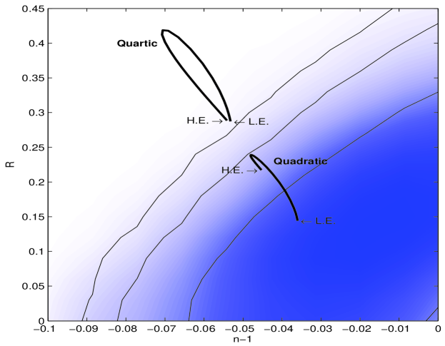
Figure 6: Constraints from WMAP data on inflation models with quadratic and quartic potentials, where $R$ is the ratio of tensor to scalar amplitudes and $n$ is the scalar spectral index. The high energy (H.E.) and low energy (L.E.) limits are shown, with intermediate energies in between, and the 1-$\sigma$ and 2-$\sigma$ contours are also shown. (From lidsmi .)

Other perturbation modes have also been investigated:

• High-energy inflation on the brane also generates a zero-mode (4D graviton mode) of tensor perturbations, and stretches it to super-Hubble scales, as will be discussed below. This zero-mode has the same qualitative features as in general relativity, remaining frozen at constant amplitude while beyond the Hubble horizon. Its amplitude is enhanced at high energies, although the enhancement is much less than for scalar perturbations lmw :

  $$A_{\rm t}^{2} \approx \left({32V\over 75M_{\rm p}^{2}}\right)\left[{3V^{2}\over 4\lambda^{2}}\right],$$ (219)

  $${A_{\rm t}^{2}\over A_{\rm s}^{2}} \approx \left({M_{\rm p}^{2}\over 16\pi}\,{V^{\prime 2}\over V^{2}}\right)\left[{6\lambda\over V}\right].$$ (220)

  Equation (220) means that brane-world effects suppress the large-scale tensor contribution to CMB anisotropies. The tensor spectral index at high energy has a smaller magnitude than in general relativity,

  $$n_{\rm t}=-3\epsilon\,,$$ (221)

  but remarkably the same consistency relation as in general relativity holds hulid1 :

  $$n_{\rm t}=-2{A_{\rm t}^{2}\over A_{\rm s}^{2}}\,.$$ (222)

  This consistency relation persists when $Z_{2}$ symmetry is dropped hulid2 (and in a two-brane model with stabilized radion gklr ). It holds only to lowest order in slow-roll, as in general relativity, but the reason for this seetay and the nature of the corrections cal are not settled.

  The massive KK modes of tensor perturbations remain in the vacuum state during slow-roll inflation lmw ; grs . The evolution of the super-Hubble zero mode is the same as in general relativity, so that high-energy brane-world effects in the early universe serve only to rescale the amplitude. However, when the zero mode re-enters the Hubble horizon, massive KK modes can be excited.

• Vector perturbations in the bulk metric can support vector metric perturbations on the brane, even in the absence of matter perturbations (see the next section). However, there is no normalizable zero mode, and the massive KK modes stay in the vacuum state during brane-world inflation bmwv . Therefore, as in general relativity, we can neglect vector perturbations in inflationary cosmology.

Brane-world effects on large-scale isocurvature perturbations in 2-field inflation have also been considered abd . Brane-world (p)reheating after inflation is discussed in preheat .

V.2 Brane-world instanton

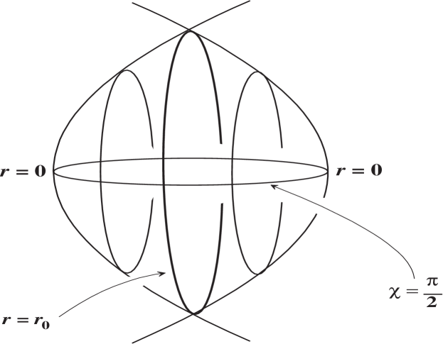
Figure 7: Brane-world instanton. (From gs .)

The creation of an inflating brane-world can be modelled as a de Sitter instanton in a way that closely follows the 4D instanton, as shown in gs . The instanton consists of two identical patches of AdS₅ joined together along a dS₄ brane with compact spatial sections. The instanton describes the “birth” of both the inflating brane and the bulk spacetime, which are together “created from nothing”, i.e. the point at the south pole of the de Sitter 4-sphere. The Euclidean AdS₅ metric is

$${}^{(5)}\!ds^{2}_{\rm euclid}=dr^{2}+\ell^{2}\sinh^{2}(r/\ell)\left[d\chi^{2}+\sin^{2}\chi\,d\Omega^{2}_{(3)}\right]\,,$$ (223)

where $d\Omega^{2}_{(3)}$ is a 3-sphere, and $r\leq r_{0}$. The Euclidean instanton interpolates between $r=0$ (“nothing”) and $r=r_{0}$ (the created universe), which is a spherical brane of radius

$$H_{0}^{-1}\equiv\ell\sinh(r_{0}/\ell)\,.$$ (224)

After creation, the brane-world evolves according to the Lorentzian continuation, $\chi\to iH_{0}t+\pi/2$,

$${}^{(5)}\!ds^{2}=dr^{2}+(\ell H_{0})^{2}\sinh^{2}(r/\ell)\left[-dt^{2}+H_{0}^{-2}\cosh^{2}(H_{0}t)\,d\Omega^{2}_{(3)}\right]\,.$$ (225)

(See Fig. 7.)

V.3 Models with non-empty bulk

The single-brane cosmological model can be generalized to include stresses other than $\Lambda_{5}$ in the bulk.

• The simplest example arises from considering a charged bulk black hole, leading to the Reissner-Nordström AdS₅ bulk metric bv . This has the form of Eq. (180), with

  $$F(R)=K+{R^{2}\over\ell^{2}}-{m\over R^{2}}+{q^{2}\over R^{4}}\,,$$ (226)

  where $q$ is the “electric” charge parameter of the bulk black hole. The metric is a solution of the 5D Einstein-Maxwell equations, so that ${}^{(5)}\!T_{AB}$ in Eq. (46) is the energy-momentum tensor of a radial static 5D “electric” field. In order for the field lines to terminate on the boundary brane, the brane should carry a charge $-q$. Since the RNAdS₅ metric is 4-isotropic, it is still possible to embed a FRW brane in it, which is moving in the coordinates of Eq. (180).

  The effect of the black hole charge on the brane arises via the junction conditions and leads to the modified Friedmann equation bv ,

  $$H^{2}=\frac{\kappa^{2}}{3}\rho\left(1+{\rho\over 2\lambda}\right)+{m\over a^{4}}-{q^{2}\over a^{6}}+\frac{1}{3}\Lambda-\frac{K}{a^{2}}\,.$$ (227)

  The field lines that terminate on the brane imprint on the brane an effective negative energy density $-3q^{2}/(\kappa^{2}a^{6})$, which redshifts like stiff matter ($w=1$). The negativity of this term introduces the possibility that at high energies it can bring the expansion rate to zero and cause a turn-around or bounce (but see hovmy for problems with such bounces).

  Apart from negativity, the key difference between this “dark stiff matter” and the dark radiation term $m/a^{4}$, is that the latter arises from the bulk Weyl curvature via the ${\cal E}_{\mu\nu}$ tensor, while the former arises from non-vacuum stresses in the bulk via the ${\cal F}_{\mu\nu}$ tensor in Eq. (65). The dark stiff matter does not arise from massive KK modes of the graviton.

• Another example is provided by the Vaidya-AdS₅ metric, which can be written after transforming to a new coordinate $v=T+\int dR/F$ in Eq. (180), so that $v=\,$const are null surfaces, and

  $${}^{(5)}\!ds^{2} = -F(R,v)dv^{2}+2dvdR+R^{2}\left({dr^{2}\over 1-Kr^{2}}+r^{2}d\Omega^{2}\right)\,,$$ (228)

  $$F(R,v) = K+{R^{2}\over\ell^{2}}-{m(v)\over R^{2}}\,.$$ (229)

  This model has a moving FRW brane in a 4-isotropic bulk (which is not static), with either a radiating bulk black hole ($dm/dv<0$), or a radiating brane ($dm/dv>0$) ckn . The metric satisfies the 5D field equations (46) with a null-radiation energy-momentum tensor,

  $${}^{(5)}\!T_{AB}=\psi k_{A}k_{B}\,,~{}k_{A}k^{A}=0\,,~{}k_{A}u^{A}=1\,,$$ (230)

  where $\psi\propto dm/dv$. It follows that

  $${\cal F}_{\mu\nu}=\kappa_{5}^{-2}\psi h_{\mu\nu}\,.$$ (231)

  In this case, the same effect, i.e. a varying mass parameter $m$, contributes to both ${\cal E}_{\mu\nu}$ and ${\cal F}_{\mu\nu}$ in the brane field equations. The modified Friedmann equation has the standard 1-brane RS-type form, but with a dark radiation term that no longer behaves strictly like radiation:

  $$H^{2}=\frac{\kappa^{2}}{3}\rho\left(1+{\rho\over 2\lambda}\right)+{m(t)\over a^{4}}+\frac{1}{3}\Lambda-\frac{K}{a^{2}}\,.$$ (232)

  By Eqs. (70) and (230), we arrive at the matter conservation equations,

  $$\nabla^{\nu}T_{\mu\nu}=-2\psi u_{\mu}\,.$$ (233)

  This shows how the brane loses ($\psi>0$) or gains ($\psi<0$) energy in exchange with the bulk black hole. For an FRW brane, this equation reduces to

  $$\dot{\rho}+3H(\rho+p)=-2\psi\,.$$ (234)

  The evolution of $m$ is governed by the 4D contracted Bianchi identity, using Eq. (231):

  $$\nabla^{\mu}{\cal E}_{\mu\nu}={6\kappa^{2}\over\lambda}\,\nabla^{\mu}{\cal S}_{\mu\nu}+{2\over 3}\left[\kappa_{5}^{2}\left(\dot{\psi}+\Theta\psi\right)-3\kappa^{2}\psi\right]u_{\mu}+{2\over 3}\kappa_{5}^{2}\vec{\nabla}_{\mu}\psi\,.$$ (235)

  For an FRW brane, this yields

  $$\dot{\rho}_{\cal E}+4H\rho_{{\cal E}}=2\psi-{2\over 3}{\kappa_{5}^{2}\over\kappa^{2}}\left(\dot{\psi}+3H\psi\right)\,,$$ (236)

  where $\rho_{{\cal E}}=3m(t)/(\kappa^{2}a^{4})$.

• A more complicated bulk metric arises when there is a self-interacting scalar field $\Phi$ in the bulk mw ; sca . In the simplest case, when there is no coupling between the bulk field and brane matter, this gives

  $${}^{(5)}\!T_{AB}=\Phi_{,A}\Phi_{,B}-{}^{(5)}\!g_{AB}\left[V(\Phi)+{1\over 2}\,{}^{(5)}\!g^{CD}\Phi_{,C}\Phi_{,D}\right]\,,$$ (237)

  where $\Phi(x,y)$ satisfies the 5D Klein-Gordon equation,

  $${}^{(5)}\!\Box\Phi-V^{\prime}(\Phi)=0\,.$$ (238)

  The junction conditions on the field imply that

  $$\partial_{y}\Phi(x,0)=0\,.$$ (239)

  Then Eqs. (70) and (237) show that matter conservation continues to hold on the brane in this simple case:

  $$\nabla^{\nu}T_{\mu\nu}=0\,.$$ (240)

  From Eq. (237) one finds that

  $${\cal F}_{\mu\nu}={1\over 4\kappa_{5}^{2}}\left[4\phi_{,\mu}\phi_{,\nu}-g_{\mu\nu}\left\{3V(\phi)+{5\over 2}g^{\alpha\beta}\phi_{,\alpha}\phi_{,\beta}\right\}\right]\,,$$ (241)

  where

  $$\phi(x)=\Phi(x,0)\,,$$ (242)

  so that the modified Friedmann equation becomes

  $$H^{2}=\frac{\kappa^{2}}{3}\rho\left(1+{\rho\over 2\lambda}\right)+{m\over a^{4}}+{\kappa_{5}^{2}\over 6}\left[{1\over 2}\dot{\phi}^{2}+V(\phi)\right]+\frac{1}{3}\Lambda-\frac{K}{a^{2}}\,.$$ (243)

  When there is coupling between brane matter and the bulk scalar field, then the Friedmann and conservation equations are more complicated mw ; sca .

VI Brane-world cosmology: perturbations

The background dynamics of brane-world cosmology are simple because the FRW symmetries simplify the bulk and rule out nonlocal effects. But perturbations on the brane immediately release the nonlocal KK modes. Then the 5D bulk perturbation equations must be solved in order to solve for perturbations on the brane. These 5D equations are partial differential equations for the 3D Fourier modes, with both initial and boundary conditions needed.

The theory of gauge-invariant perturbations in brane-world cosmology has been extensively investigated and developed m1 ; lmsw ; bm ; mwbh ; steep ; gm ; lmw ; grs ; mu ; pert ; bmw ; l1 ; l2 and is qualitatively well understood. The key remaining task is integration of the coupled brane-bulk perturbation equations. Special cases have been solved, where these equations effectively decouple lmsw ; bm ; l1 ; l2 , and approximation schemes have recently been developed sod ; koy ; rbbd ; kkt ; elmw ; mbb for the more general cases where the coupled system must be solved. From the brane viewpoint, the bulk effects, i.e., the high-energy corrections and the KK modes, act as source terms for the brane perturbation equations. At the same time, perturbations of matter on the brane can generate KK modes (i.e., emit 5D gravitons into the bulk) which propagate in the bulk and can subsequently interact with the brane. This nonlocal interaction amongst the perturbations is at the core of the complexity of the problem. It can be elegantly expressed via integro-differential equations mu , which take the form (assuming no incoming 5D gravitational waves)

$$A_{k}(t)=\int dt^{\prime}\,{\cal G}(t,t^{\prime})B_{k}(t^{\prime})\,,$$ (244)

where ${\cal G}$ is the bulk retarded Green’s function evaluated on the brane, and $A_{k},B_{k}$ are made up of brane metric and matter perturbations and their (brane) derivatives, and include high-energy corrections to the background dynamics. Solving for the bulk Green’s function, which then determines ${\cal G}$, is the core of the 5D problem.

We can isolate the KK anisotropic stress $\pi^{{\cal E}}_{\mu\nu}$ as the term that must be determined from 5D equations. Once $\pi^{{\cal E}}_{\mu\nu}$ is determined in this way, the perturbation equations on the brane form a closed system. The solution will be of the form, expressed in Fourier modes:

$$\pi^{\cal E}_{k}(t)\propto\int dt^{\prime}\,\,{\cal G}(t,t^{\prime})F_{k}(t^{\prime})\,,$$ (245)

where the functional $F_{k}$ will be determined by the covariant brane perturbation quantities and their derivatives. It is known in the case of a Minkowski background ssm , but not in the cosmological case.

The KK terms act as source terms modifying the standard general relativity perturbation equations, together with the high-energy corrections. For example, the linearization of the shear propagation equation (127) yields

$$\dot{\sigma}_{\mu\nu}+2H\sigma_{\mu\nu}+E_{\mu\nu}-{\kappa^{2}\over 2}\pi_{\mu\nu}-\vec{\nabla}_{\langle\mu}A_{\nu\rangle}={\kappa^{2}\over 2}\pi^{{\cal E}}_{\mu\nu}-{\kappa^{2}\over 4}(1+3w){\rho\over\lambda}\,\pi_{\mu\nu}\,.$$ (246)

In 4D general relativity, the right hand side is zero. In the brane-world, the first source term on the right is the KK term, the second term is the high-energy modification. The other modification is a straightforward high-energy correction of the background quantities $H$ and $\rho$ via the modified Friedmann equations.

As in 4D general relativity, there are various different, but essentially equivalent, ways to formulate linear cosmological perturbation theory. First I describe the covariant brane-based approach.

VI.1 1+3-covariant perturbation equations on the brane

In the 1+3-covariant approach m1 ; l1 ; mjap , perturbative quantities are projected vectors, $V_{\mu}=V_{\langle\mu\rangle}$, and projected symmetric tracefree tensors, $W_{\mu\nu}=W_{\langle\mu\nu\rangle}$, which are gauge-invariant since they vanish in the background. These are decomposed into (3D) scalar, vector and tensor modes as

$$V_{\mu} = \vec{\nabla}_{\mu}V+\bar{V}_{\mu}\,,$$ (247)

$$W_{\mu\nu} = \vec{\nabla}_{\langle\mu}\vec{\nabla}_{\nu\rangle}{W}+\vec{\nabla}_{\langle\mu}\bar{W}_{\nu\rangle}+\bar{W}_{\mu\nu}\,,$$ (248)

where $\bar{W}_{\mu\nu}=\bar{W}_{\langle\mu\nu\rangle}$ and an overbar denotes a (3D) transverse quantity,

$$\vec{\nabla}^{\mu}\bar{V}_{\mu}=0=\vec{\nabla}^{\nu}\bar{W}_{\mu\nu}\,.$$ (249)

In a local inertial frame comoving with $u^{\mu}$, i.e., $u^{\mu}=(1,\vec{0})$, all time components may be set to zero: $V_{\mu}=(0,V_{i})$, $W_{0\mu}=0$, $\vec{\nabla}_{\mu}=(0,\vec{\nabla}_{i})$.

Purely scalar perturbations are characterized by the fact that vectors and tensors are derived from scalar potentials, i.e.,

$$\bar{V}_{\mu}=\bar{W}_{\mu}=\bar{W}_{\mu\nu}=0\,.$$ (250)

Scalar perturbative quantities are formed from the potentials via the (3D) Laplacian, e.g., ${\cal V}=\vec{\nabla}^{\mu}\vec{\nabla}_{\mu}V\equiv\vec{\nabla}^{2}V$. Purely vector perturbations are characterized by

$$V_{\mu}=\bar{V}_{\mu}\,,~{}W_{\mu\nu}=\vec{\nabla}_{\langle\mu}\bar{W}_{\nu\rangle}\,,~{}\mbox{curl}\,\vec{\nabla}_{\mu}f=-2\dot{f}\omega_{\mu}\,,$$ (251)

where $\omega_{\mu}$ is the vorticity, and purely tensor by

$$\vec{\nabla}_{\mu}f=0=V_{\mu}\,,~{}W_{\mu\nu}=\bar{W}_{\mu\nu}\,.$$ (252)

The KK energy density produces a scalar mode $\vec{\nabla}_{\mu}{\rho_{{\cal E}}}$ (which is present even if $\rho_{{\cal E}}=0$ in the background). The KK momentum density carries scalar and vector modes, and the KK anisotropic stress carries scalar, vector and tensor modes:

$${q^{{\cal E}}_{\mu}} = \vec{\nabla}_{\mu}q^{{\cal E}}+{\bar{q}^{{\cal E}}_{\mu}}\,,$$ (253)

$${\pi^{{\cal E}}_{\mu\nu}} = \vec{\nabla}_{\langle\mu}\vec{\nabla}_{\nu\rangle}\pi^{{\cal E}}+\vec{\nabla}_{\langle\mu}{\bar{\pi}^{{\cal E}}_{\nu\rangle}}+{\bar{\pi}^{{\cal E}}_{\mu\nu}}\,.$$ (254)

Linearizing the conservation equations for a single adiabatic fluid, and the nonlocal conservation equations, we obtain

$$\dot{\rho}+\Theta(\rho+p)=0\,,$$ (255)

$$c_{\rm s}^{2}\vec{\nabla}_{\mu}+(\rho+p)A_{\mu}=0\,,$$ (256)

$$\dot{\rho}_{\cal E}+{4\over 3}\Theta{\rho_{{\cal E}}}+\vec{\nabla}^{\mu}{q^{{\cal E}}_{\mu}}=0\,,$$ (257)

$$\dot{q}^{\cal E}_{\mu}+4H{q^{{\cal E}}_{\mu}}+{{1\over 3}}\vec{\nabla}_{\mu}{\rho_{{\cal E}}}+{{4\over 3}}{\rho_{{\cal E}}}A_{\mu}+\vec{\nabla}^{\nu}{\pi^{{\cal E}}_{\mu\nu}}=-{(\rho+p)\over\lambda}\vec{\nabla}_{\mu}\rho\,.$$ (258)

Linearizing the remaining propagation and constraint equations leads to

$$\dot{\Theta}+{{1\over 3}}\Theta^{2}-\vec{\nabla}^{\mu}A_{\mu}+{{1\over 2}}\kappa^{2}(\rho+3p)-\Lambda=-{{\kappa^{2}\over 2}}(2\rho+3p){\rho\over\lambda}-\kappa^{2}\rho_{{\cal E}}\,,$$ (259)

$$\dot{\omega}_{\mu}+2H\omega_{\mu}+{{1\over 2}}\mbox{curl}\,A_{\mu}=0\,,$$ (260)

$$\dot{\sigma}_{\mu\nu}+2H\sigma_{\mu\nu}+E_{\mu\nu}-\vec{\nabla}_{\langle\mu}A_{\nu\rangle}={\kappa^{2}\over 2}\pi^{{\cal E}}_{\mu\nu}\,,$$ (261)

$$\dot{E}_{\mu\nu}+3HE_{\mu\nu}-\mbox{curl}\,H_{\mu\nu}+{{\kappa^{2}\over 2}}(\rho+p)\sigma_{\mu\nu}=-{{\kappa^{2}\over 2}}(\rho+p){\rho\over\lambda}\sigma_{\mu\nu}$$

$$~{}~{}{}-{\kappa^{2}\over 6}\left[4\rho_{{\cal E}}\sigma_{\mu\nu}+3\dot{\pi}^{\cal E}_{\mu\nu}+3H\pi^{{\cal E}}_{\mu\nu}+3\vec{\nabla}_{\langle\mu}q^{{\cal E}}_{\nu\rangle}\right]\,,$$ (262)

$$\dot{H}_{\mu\nu}+3HH_{\mu\nu}+\mbox{curl}\,E_{\mu\nu}={\kappa^{2}\over 2}\mbox{curl}\,\pi^{{\cal E}}_{\mu\nu}\,,$$ (263)

$$\vec{\nabla}^{\mu}\omega_{\mu}=0\,,$$ (264)

$$\vec{\nabla}^{\nu}\sigma_{\mu\nu}-\mbox{curl}\,\omega_{\mu}-{{2\over 3}}\vec{\nabla}_{\mu}\Theta=-q^{{\cal E}}_{\mu}\,,$$ (265)

$$\mbox{curl}\,\sigma_{\mu\nu}+\vec{\nabla}_{\langle\mu}\omega_{\nu\rangle}-H_{\mu\nu}=0\,,$$ (266)

$$\vec{\nabla}^{\nu}E_{\mu\nu}-{{\kappa^{2}\over 3}}\vec{\nabla}_{\mu}\rho={\kappa^{2}\over 3}{\rho\over\lambda}\vec{\nabla}_{\mu}\rho+{\kappa^{2}\over 6}\left[2\vec{\nabla}_{\mu}\rho_{{\cal E}}-4Hq^{{\cal E}}_{\mu}-3\vec{\nabla}^{\nu}\pi^{{\cal E}}_{\mu\nu}\right]\,,$$ (267)

$$\vec{\nabla}^{\nu}H_{\mu\nu}-\kappa^{2}(\rho+p)\omega_{\mu}=\kappa^{2}(\rho+p){\rho\over\lambda}\omega_{\mu}+{\kappa^{2}\over 6}\left[8\rho_{{\cal E}}\omega_{\mu}-3\mbox{curl}\,q^{{\cal E}}_{\mu}\right]\,.$$ (268)

Equations (255), (257) and (259) do not provide gauge-invariant equations for perturbed quantities, but their spatial gradients do.

These equations are the basis for a 1+3-covariant analysis of cosmological perturbations from the brane observer’s viewpoint, following the approach developed in 4D general relativity covp . The equations contain scalar, vector and tensor modes, which can be separated out if desired. They are not a closed system of equations until $\pi^{{\cal E}}_{\mu\nu}$ is determined by a 5D analysis of the bulk perturbations. An extension of the 1+3-covariant perturbation formalism to 1+4 dimensions would require a decomposition of the 5D geometric quantities along a timelike extension $u^{A}$ into the bulk of the brane 4-velocity field $u^{\mu}$, and this remains to be done. The 1+3-covariant perturbation formalism is incomplete until such a 5D extension is performed. The metric-based approach does not have this drawback.

VI.2 Metric-based perturbations

An alternative approach to brane-world cosmological perturbations is an extension of the 4D metric-based gauge-invariant theory metp . A review of this approach is given in bmw . In an arbitrary gauge, and for a flat FRW background, the perturbed metric has the form

$$\delta\,^{(5)}\!g_{AB}=\left[\begin{array}[]{ccc|c}-2N^{2}\psi&&A^{2}(\partial_{i}{\cal B}-S_{i})&N\alpha\\ &&&\\ A^{2}(\partial_{j}{\cal B}-S_{j})&&A^{2}\left\{2{\cal R}\delta_{ij}+2\partial_{i}\partial_{j}{\cal C}+2\partial_{(i}F_{j)}+f_{ij}\right\}&A^{2}(\partial_{i}\beta-\chi_{i})\\ &&&\\ \hline\cr&&&\\ N\alpha&&A^{2}(\partial_{j}\beta-\chi_{j})&2\nu\end{array}\right]\,,$$ (269)

where the background metric functions $A,N$ are given by Eqs. (183) and (184). The scalars $\psi,{\cal R},{\cal C},\alpha,\beta,\nu$ represent scalar perturbations. The vectors $S_{i},F_{i}$ and $\chi_{i}$ are transverse, so that they represent 3D vector perturbations, and the tensor $f_{ij}$ is transverse traceless, representing 3D tensor perturbations.

In the Gaussian normal gauge, the brane coordinate-position remains fixed under perturbation,

$${}^{(5)}\!ds^{2}=\left[{g}^{(0)}_{\mu\nu}(x,y)+\delta g_{\mu\nu}(x,y)\right]dx^{\mu}dx^{\nu}+dy^{2}\,,$$ (270)

where ${g}^{(0)}_{\mu\nu}$ is the background metric, Eq. (182). In this gauge,

$$\alpha=\beta=\nu=\chi_{i}=0\,.$$ (271)

In the 5D longitudinal gauge,

$$-{\cal B}+\dot{\cal C}=0=-\beta+{\cal C}^{\prime}\,.$$ (272)

In this gauge, and for an AdS₅ background, the metric perturbation quantities can all be expressed in terms of a “master variable” $\Omega$ which obeys a wave equation mu . In the case of scalar perturbations, we have for example,

$${\cal R}={1\over 6A}\left(\Omega^{\prime\prime}-{1\over N^{2}}\,\ddot{\Omega}-{\Lambda_{5}\over 3}\,\Omega\right)\,,$$ (273)

with similar expressions for the other quantities. All of the metric perturbation quantities are determined once a solution is found for the wave equation

$$\left({1\over NA^{3}}\,\dot{\Omega}\right)^{\displaystyle{\cdot}}+\left({\Lambda_{5}\over 6}+{k^{2}\over A^{2}}\right){N\over A^{3}}\,\Omega=\left({N\over A^{3}}\,\Omega^{\prime}\right)^{\prime}\,.$$ (274)

The junction conditions Eq. (64) relate the off-brane derivatives of metric perturbations to the matter perturbations:

$$\partial_{y}\,\delta g_{\mu\nu}=-\kappa^{2}_{5}\left[\delta T_{\mu\nu}+{1\over 3}\left\{\lambda-T^{(0)}\right\}\delta g_{\mu\nu}-{1\over 3}{g}^{(0)}_{\mu\nu}\delta T\right],$$ (275)

where

$$\delta T^{0}{}_{0}=-\delta\rho\,,~{}\delta T^{0}{}_{i}=a^{2}q_{i}\,,$$ (276)

$$\delta T^{i}{}_{j}=\delta p\,\delta^{i}{}_{j}+\delta\pi^{i}{}_{j}\,.$$ (277)

For scalar perturbations in the Gaussian normal gauge, this gives

$$\partial_{y}\psi(x,0) = {\kappa^{2}_{5}\over 6}(2\delta\rho+3\delta p)\,,$$ (278)

$$\partial_{y}{\cal B}(x,0) = \kappa^{2}_{5}\delta p\,,$$ (279)

$$\partial_{y}{\cal C}(x,0) = -{\kappa^{2}_{5}\over 2}\delta\pi\,,$$ (280)

$$\partial_{y}{\cal R}(x,0) = -{\kappa^{2}_{5}\over 6}\delta\rho-\partial_{i}\partial^{i}\,{\cal C}(x,0)\,,$$ (281)

where $\delta\pi$ is the scalar potential for the matter anisotropic stress,

$$\delta\pi_{ij}=\partial_{i}\partial_{j}\delta\pi-{1\over 3}\delta_{ij}\,\partial_{k}\partial^{k}\delta\pi\,.$$ (282)

The perturbed KK energy-momentum tensor on the brane is given by

$$\delta{\cal E}^{0}{}_{0}=\kappa^{2}\delta\rho_{{\cal E}}\,,~{}\delta{\cal E}^{0}{}_{i}=-\kappa^{2}a^{2}q^{{\cal E}}_{i}\,,$$ (283)

$$\delta{\cal E}^{i}{}_{j}=-{\kappa^{2}\over 3}\delta\rho_{{\cal E}}\,\delta^{i}{}_{j}-\delta\pi^{{\cal E}i}{}_{j}\,.$$ (284)

The evolution of the bulk metric perturbations is determined by the perturbed 5D field equations in the vacuum bulk,

$$\delta\,{}^{(5)}\!G^{A}{}_{B}=0\,.$$ (285)

Then the matter perturbations on the brane enter via the perturbed junction conditions, Eq. (275).

For example, for scalar perturbations in Gaussian normal gauge,

$$\delta\,{}^{(5)}\!G^{y}{}_{i} = \partial_{i}\left\{-\psi^{\prime}+\left({A^{\prime}\over A}-{N^{\prime}\over N}\right)\psi-2{\cal R}^{\prime}\right.$$ (286)

$$~{}~{}~{}~{}{}\left.-{A^{2}\over 2N^{2}}\left[\dot{\cal B}^{\prime}+\left(5{\dot{A}\over A}-{\dot{N}\over N}\right){\cal B}^{\prime}\right]\right\}\,.$$

For tensor perturbations (in any gauge), the only nonzero components of the perturbed Einstein tensor are

$$\delta\,{}^{(5)}\!G^{i}{}_{j} = -{1\over 2}\left\{-{1\over N^{2}}\ddot{f}^{i}{}_{j}+f^{\prime\prime i}{}_{j}-{k^{2}\over A^{2}}f^{i}{}_{j}\right.$$ (287)

$$~{}~{}{}\left.+{1\over N^{2}}\left({\dot{N}\over N}-3{\dot{A}\over A}\right)\dot{f}^{i}{}_{j}+\left({N^{\prime}\over N}+3{A^{\prime}\over A}\right)f^{\prime i}{}_{j}\right\}\,.$$

In the following, I will discuss various perturbation problems, using either a 1+3-covariant or a metric-based approach.

VI.3 Density perturbations on large scales

In the covariant approach, we define matter density and expansion (velocity) perturbation scalars, as in 4D general relativity,

$$\Delta={a^{2}\over\rho}\vec{\nabla}^{2}\rho\,,~{}Z=a^{2}\vec{\nabla}^{2}\Theta\,.$$ (288)

Then we can define dimensionless KK perturbation scalars m1 ,

$${U}={a^{2}\over\rho}\vec{\nabla}^{2}{\rho_{{\cal E}}}\,,~{}{Q}={a\over\rho}\vec{\nabla}^{2}q^{{\cal E}}\,,~{}{\Pi}={1\over\rho}\vec{\nabla}^{2}\pi^{{\cal E}}\,,$$ (289)

where the scalar potentials $q^{{\cal E}}$ and $\pi^{{\cal E}}$ are defined by Eqs. (253) and (254). The KK energy density (dark radiation) produces a scalar fluctuation $U$ which is present even if $\rho_{{\cal E}}=0$ in the background, and which leads to a non-adiabatic (or isocurvature) mode, even when the matter perturbations are assumed adiabatic gm . We define the total effective dimensionless entropy $S_{\rm tot}$ via

$$p_{\rm tot}\,S_{\rm tot}=a^{2}\vec{\nabla}^{2}p_{\rm tot}-c_{\rm tot}^{2}a^{2}\vec{\nabla}^{2}\rho_{\rm tot}\,,$$ (290)

where $c_{\rm tot}^{2}=\dot{p}_{\rm tot}/\dot{\rho}_{\rm tot}$ is given in Eq. (105). Then

$$S_{\rm tot}={9\left[c_{\rm s}^{2}-{1\over 3}+\left({2\over 3}+w+c_{\rm s}^{2}\right){{\rho/\lambda}}\right]\over[3(1+w)(1+\rho/\lambda)+4\rho_{{\cal E}}/\rho][3w+3(1+2w)\rho/2\lambda+\rho_{{\cal E}}/\rho]}\,\left[{4\over 3}{\rho_{{\cal E}}\over\rho}\,\Delta-(1+w)U\right]\,.$$ (291)

If $\rho_{{\cal E}}=0$ in the background, then $U$ is an isocurvature mode: $S_{\rm tot}\propto(1+w)U$. This isocurvature mode is suppressed during slow-roll inflation, when $1+w\approx 0$.

If $\rho_{{\cal E}}\neq 0$ in the background, then the weighted difference between $U$ and $\Delta$ determines the isocurvature mode: $S_{\rm tot}\propto(4\rho_{{\cal E}}/3\rho)\Delta-(1+w)U$. At very high energies, $\rho\gg\lambda$, the entropy is suppressed by the factor $\lambda/\rho$.

The density perturbation equations on the brane are derived by taking the spatial gradients of Eqs. (255), (257) and (259), and using Eqs. (256) and (258). This leads to gm

$$\dot{\Delta} = 3wH\Delta-(1+w)Z\,,$$ (292)

$$\dot{Z} = -2HZ-\left({c_{\rm s}^{2}\over 1+w}\right)\vec{\nabla}^{2}\Delta-\kappa^{2}\rho{U}-{{1\over 2}}\kappa^{2}\rho\left[1+(4+3w){{\rho\over\lambda}}-\left({4c_{\rm s}^{2}\over 1+w}\right){\rho_{{\cal E}}\over\rho}\right]\Delta\,,$$ (293)

$${\dot{U}} = (3w-1)H{U}+\left({4c_{\rm s}^{2}\over 1+w}\right)\left({{\rho_{{\cal E}}}\over\rho}\right)H\Delta-\left({4{\rho_{{\cal E}}}\over 3\rho}\right)Z-a\vec{\nabla}^{2}{Q}\,,$$ (294)

$${\dot{Q}} = (3w-1)H{Q}-{1\over 3a}{U}-{{2\over 3}}a{\vec{\nabla}^{2}\Pi}+{1\over 3\mu}\left[\left({4c_{\rm s}^{2}\over 1+w}\right){{\rho_{{\cal E}}}\over\rho}-3(1+w){{\rho\over\lambda}}\right]\Delta\,.$$ (295)

The KK anisotropic stress term $\Pi$ occurs only via its Laplacian, ${\vec{\nabla}^{2}\Pi}$. If we can neglect this term on large scales, then the system of density perturbation equations closes on super-Hubble scales m1 . An equivalent statement applies to the large-scale curvature perturbations lmsw . KK effects then introduce two new isocurvature modes on large scales (associated with $U$ and $Q$), as well as modifying the evolution of the adiabatic modes gm ; l1 .

Thus on large scales the system of brane equations is closed, and we can determine the density perturbations without solving for the bulk metric perturbations.

Figure 8: The evolution of the covariant variable $\Phi$, defined in Eq. (298) (and not to be confused with the Bardeen potential), along a fundamental world-line. This is a mode that is well beyond the Hubble horizon at $N=0$, about 50 e-folds before inflation ends, and remains super-Hubble through the radiation era. A smooth transition from inflation to radiation is modelled by $w={1\over 3}[(2-{3\over 2}\epsilon)\tanh(N-50)-(1-{3\over 2}\epsilon)]$, where $\epsilon$ is a small positive parameter (chosen as $\epsilon=0.1$ in the plot). Labels on the curves indicate the value of $\rho_{0}/\lambda$, so that the general relativistic solution is the dashed curve ($\rho_{0}/\lambda=0$). (From gm .)

We can simplify the system as follows. The 3-Ricci tensor defined in Eq. (136) leads to a scalar covariant curvature perturbation variable,

$$C\equiv a^{4}\vec{\nabla}^{2}R^{\perp}=-4a^{2}HZ+2\kappa^{2}a^{2}\rho\left(1+{\rho\over 2\lambda}\right)\Delta+2\kappa^{2}a^{2}\rho U\,.$$ (296)

It follows that $C$ is locally conserved (along $u^{\mu}$ flow lines):

$$C=C_{0}\,,~{}\dot{C}_{0}=0\,.$$ (297)

We can further simplify the system of equations via the variable

$$\Phi=\kappa^{2}a^{2}\rho\Delta\,.$$ (298)

This should not be confused with the Bardeen metric perturbation variable $\Phi_{H}$, although it is the covariant analogue of $\Phi_{H}$ in the general relativity limit. In the brane-world, high-energy and KK effects mean that $\Phi_{H}$ is a complicated generalization of this expression l1 , involving $\Pi$, but the simple $\Phi$ above is still useful to simplify the system of equations. Using these new variables, we find the closed system for large-scale perturbations:

$$\dot{\Phi} = -H\left[1+(1+w){\kappa^{2}\rho\over 2H^{2}}\left(1+{\rho\over\lambda}\right)\right]\Phi-\left[(1+w){a^{2}\kappa^{4}\rho^{2}\over 2H}\right]U+\left[(1+w){\kappa^{2}\rho\over 4H}\right]C_{0}\,,$$ (299)

$$\dot{U} = -H\left[1-3w+{2\kappa^{2}{\rho_{{\cal E}}}\over 3H^{2}}\right]U-{2{\rho_{{\cal E}}}\over 3a^{2}H\rho}\left[1+{\rho\over\lambda}-{6c_{\rm s}^{2}H^{2}\over(1+w)\kappa^{2}\rho}\right]\Phi+\left[{{\rho_{{\cal E}}}\over 3a^{2}H\rho}\right]C_{0}\,.$$ (300)

If there is no dark radiation in the background, $\rho_{{\cal E}}=0$, then

$$U=U_{0}\exp-\int(1-3w)dN\,,$$ (301)

and the above system reduces to a single equation for $\Phi$. At low energies, and for constant $w$, the non-decaying attractor is the general relativity solution,

$$\Phi_{\rm low}\approx{3(1+w)\over 2(5+3w)}\,C_{0}\,.$$ (302)

At very high energies, for $w\geq-{1\over 3}$,

$$\Phi_{\rm high}\to{3\over 2}{\lambda\over\rho_{0}}(1+w)\left[{C_{0}\over 7+6w}-{2\tilde{U}_{0}\over 5+6w}\right]\,,$$ (303)

where $\tilde{U}_{0}=\kappa^{2}a_{0}^{2}\rho_{0}U_{0}$, so that the isocurvature mode has an influence on $\Phi$. Initially, $\Phi$ is suppressed by the factor $\lambda/\rho_{0}$, but then it grows, eventually reaching the attractor value in Eq. (302). For slow-roll inflation, when $1+w\sim\epsilon$, with $0<\epsilon\ll 1$ and $H^{-1}|\dot{\epsilon}|=|\epsilon^{\prime}|\ll 1$,

$$\Phi_{\rm high}\sim{3\over 2}\epsilon{\lambda\over\rho_{0}}C_{0}e^{3\epsilon N}\,,$$ (304)

where $N=\ln(a/a_{0})$, so that $\Phi$ has a growing-mode in the early universe. This is different from general relativity, where $\Phi$ is constant during slow-roll inflation. Thus more amplification of $\Phi$ can be achieved than in general relativity, as discussed above. This is illustrated for a toy model of inflation-to-radiation in Fig. 8. The early (growing) and late time (constant) attractor solutions are seen explicitly in the plots.

Figure 9: The evolution of $\Phi$ in the radiation era, with dark radiation present in the background. (From ggm .)

The presence of dark radiation in the background introduces new features. In the radiation era ($w={1\over 3}$), the non-decaying low-energy attractor becomes ggm

$$\Phi_{\rm low} \approx {C_{0}\over 3}(1-\alpha)\,,$$ (305)

$$\alpha = {\rho_{{\cal E}}\over\rho}\lesssim 0.05\,.$$ (306)

The dark radiation serves to reduce the final value of $\Phi$, leaving an imprint on $\Phi$, unlike the $\rho_{{\cal E}}=0$ case, Eq. (302). In the very high energy limit,

$$\Phi_{\rm high} \to {\lambda\over\rho_{0}}\left[{2\over 9}C_{0}-{4\over 7}\tilde{U}_{0}\right]+16\alpha\left({\lambda\over\rho_{0}}\right)^{2}\left[{C_{0}\over 273}-{4\tilde{U}_{0}\over 539}\right]\,.$$ (307)

Thus $\Phi$ is initially suppressed, then begins to grow, as in the no-dark-radiation case, eventually reaching an attractor which is less than the no-dark-radiation attractor. This is confirmed by the numerical integration shown in Fig. 9.

VI.4 Curvature perturbations and the Sachs-Wolfe effect

The curvature perturbation ${\cal R}$ on uniform density surfaces is defined in Eq. (269). The associated gauge-invariant quantity

$$\zeta={\cal R}+{\delta\rho\over 3(\rho+p)}\,,$$ (308)

may be defined for matter on the brane. Similarly, for the Weyl “fluid” if $\rho_{{\cal E}}\neq 0$ in the background, the curvature perturbation on hypersurfaces of uniform dark energy density is

$$\zeta_{\cal E}={\cal R}+{\delta\rho_{\cal E}\over 4\rho_{{\cal E}}}\,.$$ (309)

On large scales, the perturbed dark energy conservation equation is lmsw

$$(\delta\rho_{{\cal E}})^{\displaystyle{\cdot}}+4H\delta\rho_{{\cal E}}+4\rho_{{\cal E}}\dot{\cal R}=0\,,$$ (310)

which leads to

$$\dot{\zeta}_{\cal E}=0\,.$$ (311)

For adiabatic matter perturbations, by the perturbed matter energy conservation equation,

$$(\delta\rho)^{\displaystyle{\cdot}}+3H(\delta\rho+\delta p)+3(\rho+p)\dot{\cal R}=0\,,$$ (312)

we find

$$\dot{\zeta}=0\,.$$ (313)

This is independent of brane-world modifications to the field equations, since it depends on energy conservation only. For the total, effective fluid, the curvature perturbation is defined as follows lmsw : if $\rho_{{\cal E}}\neq 0$ in the background,

$${\zeta}_{\rm tot} = {\zeta}+\left[{4\rho_{{\cal E}}\over 3(\rho+p)(1+\rho/\lambda)+4\rho_{{\cal E}}}\right]\left(\zeta_{\cal E}-\zeta\right)\,,$$ (314)

and if $\rho_{{\cal E}}=0$ in the background,

$${\zeta}_{\rm tot} = {\zeta}+{\delta\rho_{{\cal E}}\over 3(\rho+p)(1+\rho/\lambda)}$$ (315)

$$\delta\rho_{{\cal E}} = {\delta C_{\cal E}\over a^{4}}\,,$$ (316)

where $\delta C_{\cal E}$ is a constant. It follows that the curvature perturbations on large scales, like the density perturbations, can be found on the brane without solving for the bulk metric perturbations.

Note that $\dot{\zeta}_{\rm\,tot}\neq 0$ even for adiabatic matter perturbations; for example, if $\rho_{{\cal E}}=0$ in the background,

$$\dot{\zeta}_{\rm\,tot}=H\left(c_{\rm tot}^{2}-{1\over 3}\right){\delta\rho_{{\cal E}}\over(\rho+p)(1+\rho/\lambda)}\,.$$ (317)

The KK effects on the brane contribute a non-adiabatic mode, although $\dot{\zeta}_{\rm\,tot}\to 0$ at low energies.

Although the density and curvature perturbations can be found on super-Hubble scales, the Sachs-Wolfe effect requires $\pi^{{\cal E}}_{\mu\nu}$ in order to translate from density/ curvature to metric perturbations. In the 4D longitudinal gauge of the metric perturbation formalism, the gauge-invariant curvature and metric perturbations on large scales are related by

$$\zeta_{\rm tot} = {\cal R}-{H\over\dot{H}}\left({\dot{\cal R}\over H}-\psi\right)\,,$$ (318)

$${\cal R}+\psi = -\kappa^{2}a^{2}\delta\pi_{\cal E}\,,$$ (319)

where the radiation anisotropic stress on large scales is neglected, as in general relativity, and $\delta\pi_{\cal E}$ is the scalar potential for $\pi^{{\cal E}}_{\mu\nu}$, equivalent to the covariant quantity $\Pi$ defined in Eq. (289). In 4D general relativity, the right hand side of Eq. (319) is zero. The (non-integrated) Sachs-Wolfe formula has the same form as in general relativity:

$${\delta T\over T}\Big{|}_{\rm now}=(\zeta_{\rm rad}+\psi-{\cal R})|_{\rm dec}\,.$$ (320)

The brane-world corrections to the general relativistic Sachs-Wolfe effect are then given by lmsw

$${\delta T\over T}=\left({\delta T\over T}\right)_{\rm gr}-{8\over 3}\left({\rho_{\rm rad}\over\rho_{\rm cdm}}\right)S_{\cal E}-\kappa^{2}a^{2}\delta\pi_{\cal E}+{2\kappa^{2}\over a^{5/2}}\int da\,\,a^{7/2}\,\delta\pi_{\cal E}\,,$$ (321)

where $S_{\cal E}$ is the KK entropy perturbation (determined by $\delta\rho_{{\cal E}}$). The KK term $\delta\pi_{\cal E}$ cannot be determined by the 4D brane equations, so that $\delta T/T$ cannot be evaluated on large scales without solving the 5D equations. [Equation (321) has been generalized to a 2-brane model, in which the radion makes a contribution to the Sachs-Wolfe effect ksw .]

The presence of the KK (Weyl, dark) component has essentially two possible effects.

• A contribution from the KK entropy perturbation $S_{\cal E}$ that is similar to an extra isocurvature contribution.

• The KK anisotropic stress $\delta\pi_{\cal E}$ also contributes to the CMB anisotropies. In the absence of anisotropic stresses, the curvature perturbation $\zeta_{\rm tot}$ would be sufficient to determine the metric perturbation ${\cal R}$ and hence the large-angle CMB anisotropies, via Eqs. (318), (319) and (320). However bulk gravitons generate anisotropic stresses which, although they do not affect the large-scale curvature perturbation $\zeta_{\rm tot}$, can affect the relation between $\zeta_{\rm tot}$, ${\cal R}$ and $\psi$, and hence can affect the CMB anisotropies at large angles.

A simple phenomenological approximation to $\delta\pi_{\cal E}$ on large scales is discussed in bm and the Sachs-Wolfe effect is estimated as

$${\delta T\over T}\sim\left({\delta\pi_{\cal E}\over\rho}\right)_{\!\rm in}\left({t_{\rm eq}\over t_{\rm dec}}\right)^{2/3}\left[{\ln(t_{\rm in}/t_{4})\over\ln(t_{\rm eq}/t_{4})}\right],$$ (322)

where $t_{4}$ is the 4D Planck time and $t_{\rm in}$ is the time when the KK anisotropic stress is induced on the brane, which is expected to be of the order of the 5D Planck time.

A self-consistent approximation is developed in koy , using the low-energy 2-brane approximation sod to find an effective 4D form for ${\cal E}_{\mu\nu}$ and hence for $\delta\pi_{\cal E}$. This is discussed below.

VI.5 Vector perturbations

The vorticity propagation equation on the brane is the same as in general relativity,

$$\dot{\omega}_{\mu}+2H\omega_{\mu}=-{1\over 2}\mbox{curl}\,A_{\mu}\,.$$ (323)

Taking the curl of the conservation equation (108) (for the case of a perfect fluid, $q_{\mu}=0=\pi_{\mu\nu}$), and using the identity in Eq. (251), one obtains

$$\mbox{curl}\,A_{\mu}=-6Hc_{\rm s}^{2}\omega_{\mu}\,,$$ (324)

as in general relativity, so that Eq. (323) becomes

$$\dot{\omega}_{\mu}+\left(2-3c_{\rm s}^{2}\right)H\omega_{\mu}=0\,,$$ (325)

which expresses the conservation of angular momentum. In general relativity, vector perturbations vanish when the vorticity is zero. By contrast, in brane-world cosmology, bulk KK effects can source vector perturbations even in the absence of vorticity m2 . This can be seen via the divergence equation for the magnetic part $H_{\mu\nu}$ of the 4D Weyl tensor on the brane:

$$\vec{\nabla}^{2}\bar{H}_{\mu}=2\kappa^{2}(\rho+p)\left[1+{{\rho\over\lambda}}\right]\omega_{\mu}+{4\over 3}\kappa^{2}{\rho_{{\cal E}}}\omega_{\mu}-{1\over 2}\kappa^{2}\mbox{curl}\,{\bar{q}^{{\cal E}}_{\mu}}\,,$$ (326)

where $H_{\mu\nu}=\vec{\nabla}_{\langle\mu}\bar{H}_{\nu\rangle}$. Even when $\omega_{\mu}=0$, there is a source for gravimagnetic terms on the brane from the KK quantity $\mbox{curl}\,{\bar{q}^{{\cal E}}_{\mu}}$.

We define covariant dimensionless vector perturbation quantities for the vorticity and the KK gravi-vector term:

$$\bar{\alpha}_{\mu}=a\,\omega_{\mu}\,,~{}\bar{\beta}_{\mu}={a\over\rho}\mbox{curl}\,{\bar{q}^{{\cal E}}_{\mu}}\,.$$ (327)

On large scales, we can find a closed system for these vector perturbations on the brane m2 :

$$\dot{\bar{\alpha}}_{\mu}+\left(1-3c_{\rm s}^{2}\right)H\bar{\alpha}_{\mu} = 0\,,$$ (328)

$$\dot{\bar{\beta}}_{\mu}+(1-3w)H\bar{\beta}_{\mu} = {2\over 3}H\left[4\left(3c_{\rm s}^{2}-1\right){{\rho_{{\cal E}}}\over\rho}-9(1+w)^{2}{{\rho\over\lambda}}\right]\bar{\alpha}_{\mu}\,.$$ (329)

Thus we can solve for $\bar{\alpha}_{\mu}$ and $\bar{\beta}_{\mu}$ on super-Hubble scales, as for density perturbations. Vorticity in the brane matter is a source for the KK vector perturbation $\bar{\beta}_{\mu}$ on large scales. Vorticity decays unless the matter is ultra-relativistic or stiffer ($w\geq{1\over 3}$), and this source term typically provides a decaying mode. There is another pure KK mode, independent of vorticity, but this mode decays like vorticity. For $w\equiv p/\rho=\,$const, the solutions are

$$\bar{\alpha}_{\mu} = b_{\mu}\left({a\over a_{0}}\right)^{3w-1}\,,$$ (330)

$$\bar{\beta}_{\mu} = c_{\mu}\left({a\over a_{0}}\right)^{3w-1}+b_{\mu}\left[{8\rho_{{\cal E}\,0}\over 3\rho_{0}}\left({a\over a_{0}}\right)^{2(3w-1)}+2(1+w){\rho_{0}\over\lambda}\left({a\over a_{0}}\right)^{-4}\,\right]\,,$$ (331)

where $\dot{b}_{\mu}=0=\dot{c}_{\mu}$.

Inflation will redshift away the vorticity and the KK mode. Indeed, the massive KK vector modes are not excited during slow-roll inflation bmw .

VI.6 Tensor perturbations

The covariant description of tensor modes on the brane is via the shear, which satisfies the wave equation m2

$$\vec{\nabla}^{2}{\bar{\sigma}}_{\mu\nu}-\ddot{\bar{\sigma}}_{\mu\nu}-5H\dot{\bar{\sigma}}_{\mu\nu}-\left[2\Lambda+{{1\over 2}}\kappa^{2}\left\{\rho-3p-(\rho+3p){{\rho\over\lambda}}\right\}\right]{\bar{\sigma}}_{\mu\nu}$$

$$~{}~{}{}=-{\kappa^{2}}\left({\dot{\bar{\pi}}^{\cal E}_{\mu\nu}}+2H{\bar{\pi}^{{\cal E}}_{\mu\nu}}\right).$$ (332)

Unlike the density and vector perturbations, there is no closed system on the brane for large scales. The KK anisotropic stress $\bar{\pi}^{{\cal E}}_{\mu\nu}$ is an unavoidable source for tensor modes on the brane. Thus it is necessary to use the 5D metric-based formalism. This is the subject of the next section.

VII Gravitational wave perturbations in brane-world cosmology

The tensor perturbations are given by Eq. (269), i.e. (for a flat background brane),

$${}^{(5)}\!ds^{2}=-N^{2}(t,y)dt^{2}+A^{2}(t,y)\left[\delta_{ij}+f_{ij}\right]dx^{i}dx^{j}+dy^{2}\,.$$ (333)

The transverse traceless $f_{ij}$ satisfies Eq. (287), which implies, on splitting $f_{ij}$ into Fourier modes with amplitude $f(t,y)$,

$${1\over N^{2}}\left[\ddot{f}+\left(3{\dot{A}\over A}-{\dot{N}\over N}\right)\dot{f}\right]+{k^{2}\over A^{2}}f=f^{\prime\prime}+\left(3{A^{\prime}\over A}+{N^{\prime}\over N}\right)f^{\prime}\,.$$ (334)

By the transverse traceless part of Eq. (275), the boundary condition is

$$f^{\prime}_{ij}\big{|}_{\rm brane}=\bar{\pi}_{ij}\,,$$ (335)

where $\bar{\pi}_{ij}$ is the tensor part of the anisotropic stress of matter-radiation on the brane.

The wave equation (334) cannot be solved analytically except if the background metric functions are separable, and this only happens for maximally symmetric branes, i.e. branes with constant Hubble rate $H_{0}$. This includes the RS case $H_{0}=0$, already treated in Sec. II. The cosmologically relevant case is the de Sitter brane, $H_{0}>0$. We can calculate the spectrum of gravitational waves generated during brane inflation lmw ; grs ; fk ; gwtan , if we approximate slow-roll inflation by a succession of de Sitter phases. The metric for a de Sitter brane, dS₄, in AdS₅ is given by Eqs. (182)–(184) with

$$N(t,y)=n(y)\,,~{}~{}A(t,y)=a(t)n(y)\,,$$ (336)

$$n(y)=\cosh\mu y-\left(1+{\rho_{0}\over\lambda}\right)\sinh\mu|y|\,,$$ (337)

$$a(t)=a_{0}\exp{H_{0}(t-t_{0})}\,,~{}~{}H_{0}^{2}={\kappa^{2}\over 3}\rho_{0}\left(1+{\rho_{0}\over 2\lambda}\right)\,,$$ (338)

where $\mu=\ell^{-1}$.

Figure 10: Graviton “volcano” potential around the dS₄ brane, showing the mass gap (from lan ).

The linearized wave equation (334) is separable. As before, we separate the amplitude as $f=\sum\varphi_{m}(t)f_{m}(y)$ where $m$ is the 4D mass, and this leads to:

$$\ddot{\varphi}_{m}+3H_{0}\dot{\varphi}_{m}+\left[m^{2}+{k^{2}\over a^{2}}\right]\varphi_{m}=0\,,$$ (339)

$$f_{m}^{\prime\prime}+4{n^{\prime}\over n}f_{m}^{\prime}+{m^{2}\over n^{2}}f_{m}=0\,.$$ (340)

The general solutions for $m>0$ are

$$\varphi_{m}(t) = \exp\left(-{3\over 2}H_{0}t\right)B_{\nu}\left({k\over H_{0}}e^{-H_{0}t}\right)\,,$$ (341)

$$f_{m}(y) = n(y)^{-3/2}L^{\nu}_{3/2}\left(\sqrt{1+{\mu^{2}\over H_{0}^{2}}n(y)^{2}}\right)\,,$$ (342)

where $B_{\nu}$ is a linear combination of Bessel functions, $L^{\nu}_{3/2}$ is a linear combination of associated Legendre functions, and

$$\nu=i\sqrt{{m^{2}\over H_{0}^{2}}-{9\over 4}}\,.$$ (343)

It is more useful to reformulate Eq. (340) as a Schrödinger-type equation,

$${d^{2}\Psi_{m}\over dz^{2}}-V(z)\Psi_{m}=-m^{2}\Psi_{m}\,,$$ (344)

using the conformal coordinate

$$z=z_{\rm b}+\int_{0}^{y}{d{\tilde{y}}\over n({\tilde{y}})}\,,~{}~{}z_{\rm b}={1\over H_{0}}\sinh^{-1}\left({H_{0}\over\mu}\right)\,,$$ (345)

and defining $\Psi_{m}\equiv n^{3/2}f_{m}$. The potential is given by (see Fig. 10)

$$V(z)={15H_{0}^{2}\over 4\sinh^{2}(H_{0}z)}+{{9\over 4}}H_{0}^{2}-3\mu\left[1+{\rho_{0}\over\lambda}\right]\delta(z-z_{\rm b})\,,$$ (346)

where the last term incorporates the boundary condition at the brane. The “volcano” shape of the potential shows how the 5D graviton is localized at the brane at low energies. (Note that localization fails for an AdS₄ brane nonloc .)

The non-zero value of the Hubble parameter implies the existence of a mass gap gs ,

$$\Delta m={3\over 2}H_{0}\,,$$ (347)

between the zero mode and the continuum of massive KK modes. This result has been generalized: for dS₄ brane(s) with bulk scalar field, a universal lower bound on the mass gap of the KK tower is fk

$$\Delta m\geq\sqrt{3\over 2}H_{0}\,.$$ (348)

The massive modes decay during inflation, according to Eq. (341), leaving only the zero mode, which is effectively a 4D gravitational wave. The zero mode, satisfying the boundary condition,

$$f^{\prime}_{0}(x,0)=0\,,$$ (349)

is given by

$$f_{0}=\sqrt{\mu}\,\,F\!\left({H_{0}/\mu}\right)\,,$$ (350)

where the normalization condition

$$2\int_{z_{\rm b}}^{\infty}|\Psi_{0}^{2}|dz=1\,,$$ (351)

implies that the function $F$ is given by lmw

$$F\!\left(x\right)=\left\{\sqrt{1+x^{2}}-x^{2}\ln\left[{1\over x}+\sqrt{1+{1\over x^{2}}}\right]\right\}^{\!\!-1/2}\!.$$ (352)

At low energies ($H_{0}\ll\mu$), we recover the general relativity amplitude: $F\to 1$. At high energies, the amplitude is considerably enhanced:

$$H_{0}\gg\mu~{}\Rightarrow~{}F\approx\sqrt{3H_{0}\over 2\mu}\,.$$ (353)

The factor $F$ determines the modification of the gravitational wave amplitude relative to the standard 4D result:

$$A_{\rm t}^{2}=\left[{8\over M_{\rm p}^{2}}\left({H_{0}\over 2\pi}\right)^{2}\right]F^{2}(H_{0}/\mu).$$ (354)

The modifying factor $F$ can also be interpreted as change in the effective Planck mass fk .

This enhanced zero mode produced by brane inflation remains frozen outside the Hubble radius, as in general relativity, but when it re-enters the Hubble radius during radiation or matter domination, it will no longer be separated from the massive modes, since $H$ will not be constant. Instead, massive modes will be excited during re-entry. In other words, energy will be lost from the zero mode as 5D gravitons are emitted into the bulk, i.e., as massive modes are produced on the brane. A phenomenological model of the damping of the zero mode due to 5D graviton emission is given in l2 . Self-consistent low-energy approximations to compute this effect are developed in kkt ; elmw .

Figure 11: Damping of brane-world gravity waves on horizon re-entry due to massive mode generation. The solid curve is the numerical solution, the short-dashed curve the low-energy approximation, and the long-dashed curve the standard general relativity solution. $\epsilon_{\cal E}=\rho_{0}/\lambda$ and $\gamma$ is a parameter giving the location of the regulator brane. (From kkt .)

At zero order, the low-energy approximation is based on the following mbb . In the radiation era, at low energy, the background metric functions obey

$$A(t,y)\to a(t)e^{-\mu y}\,,~{}N(t,y)\to e^{-\mu y}\,.$$ (355)

To lowest order, the wave equation therefore separates, and the mode functions can be found analytically mbb . The massive modes in the bulk, $f_{m}(y)$, are the same as for a Minkowski brane. On large scales, or at late times, the mode functions on the brane are given in conformal time by

$$\varphi^{(0)}_{m}(\eta)=\eta^{-1/2}B_{1/4}\left({ma_{\rm h}^{2}\,\mu\over\sqrt{2}}\eta^{2}\right)\,,$$ (356)

where $a_{\rm h}$ marks the start of the low-energy regime ($\rho_{\rm h}=\lambda$) and $B_{\nu}$ denotes a linear combination of Bessel functions. The massive modes decay on super-Hubble scales, unlike the zero-mode. Expanding the wave equation in $\rho_{0}/\lambda$, one arrives at the first order, where mode-mixing arises. The massive modes $\varphi^{(1)}_{m}(\eta)$ on sub-Hubble scales are sourced by the initial zero mode that is re-entering the Hubble radius elmw :

$$\left({\partial^{2}\over\partial\eta^{2}}-{\partial^{2}_{\eta}a\over a}\right)a\varphi^{(1)}_{m}+{k^{2}}a\varphi^{(1)}_{m}+m^{2}a^{3}\varphi^{(1)}_{m}=-4{\rho_{0}\over\lambda}I_{m0}{k^{2}}a\varphi^{(0)}_{0}\,,$$ (357)

where $I_{m0}$ is a transfer matrix coefficient. The numerical integration of the equations kkt confirms the effect of massive mode generation and consequent damping of the zero-mode, as shown in Fig. 11.

VIII CMB anisotropies in brane-world cosmology

For the CMB anisotropies, one needs to consider a multi-component source. Linearizing the general nonlinear expressions for the total effective energy-momentum tensor, we obtain

$$\rho_{\text{tot}} = \rho\left(1+\frac{\rho}{2\lambda}+\frac{\rho_{\cal E}}{\rho}\right)\;,$$ (358)

$$p_{\text{tot }} = p+\frac{\rho}{2\lambda}(2p+\rho)+\frac{\rho_{\cal E}}{3}\;,$$ (359)

$$q^{\text{tot }}_{\mu} = q_{\mu}\left(1+\frac{\rho}{\lambda}\right)+q^{\cal E}_{\mu}\;,$$ (360)

$$\pi^{\text{tot }}_{\mu\nu} = \pi_{\mu\nu}\left(1-\frac{\rho+3p}{2\lambda}\right)+\pi^{\cal E}_{\mu\nu}\;,$$ (361)

where

$$\rho=\sum_{i}\rho_{(i)}\,,~{}p=\sum_{i}p_{(i)}\,,~{}q_{\mu}=\sum_{i}q^{(i)}_{\mu}\,,$$ (362)

are the total matter-radiation density, pressure and momentum density, and $\pi_{\mu\nu}$ is the photon anisotropic stress (neglecting that of neutrinos, baryons and CDM).

The perturbation equations in the previous section form the basis for an analysis of scalar and tensor CMB anisotropies in the brane-world. The full system of equations on the brane, including the Boltzmann equation for photons, has been given for scalar l1 and tensor l2 perturbations. But the systems are not closed, as discussed above, because of the presence of the KK anisotropic stress $\pi^{{\cal E}}_{\mu\nu}$, which acts a source term.

In the tight-coupling radiation era, the scalar perturbation equations may be decoupled to give an equation for the gravitational potential $\Phi$, defined by the electric part of the brane Weyl tensor (not to be confused with ${\cal E}_{\mu\nu}$):

$$E_{\mu\nu}=\vec{\nabla}_{\langle\mu}\vec{\nabla}_{\nu\rangle}\Phi\,.$$ (363)

In general relativity, the equation in $\Phi$ has no source term, but in the brane-world there is a source term made up of $\pi^{{\cal E}}_{\mu\nu}$ and its time-derivatives. At low energies ($\rho\ll\lambda$), and for a flat background ($K=0$), the equation is l1

$$3x\Phi_{k}^{\prime\prime}+12\Phi_{k}^{\prime}+x\Phi_{k}$$

$$~{}~{}~{}{}={\mbox{const}\over\lambda}\,\left[\pi_{k}^{{\cal E}\prime\prime}-{1\over x}\,{\pi_{k}^{{\cal E}\prime}}+\left({2\over x^{3}}-{3\over x^{2}}+{1\over x}\right)\pi^{{\cal E}}_{k}\right],$$ (364)

where $x=k/(aH)$, a prime denotes $d/dx$, and $\Phi_{k}$, $\pi^{{\cal E}}_{k}$ are the Fourier modes of $\Phi$ and $\pi^{{\cal E}}_{\mu\nu}$. In general relativity the right hand side is zero, so that the equation may be solved for $\Phi_{k}$, and then for the remaining perturbative variables, which gives the basis for initializing CMB numerical integrations. At high energies, earlier in the radiation era, the decoupled equation is fourth order l1 :

$$729x^{2}\Phi_{k}^{\prime\prime\prime\prime}+3888x\Phi_{k}^{\prime\prime\prime}+(1782+54x^{2})\Phi_{k}^{\prime\prime}+144x\Phi_{k}^{\prime}+(90+x^{2})\Phi_{k}$$

$$~{}~{}~{}{}={\mbox{const}}\,\left[243\left(\!{\pi^{{\cal E}}_{k}\over\rho}\!\right)^{\!\prime\prime\prime\prime}-{810\over x}\left(\!{\pi^{{\cal E}}_{k}\over\rho}\!\right)^{\!\prime\prime\prime}+{18(135+2x^{2})\over x^{2}}\left(\!{\pi^{{\cal E}}_{k}\over\rho}\!\right)^{\!\prime\prime}\right.$$

$$~{}~{}~{}~{}~{}{}\left.-{30(162+x^{2})\over x^{3}}\left(\!{\pi^{{\cal E}}_{k}\over\rho}\!\right)^{\!\prime}+{x^{4}+30(162+x^{2})\over x^{4}}\left(\!{\pi^{{\cal E}}_{k}\over\rho}\!\right)\right].$$ (365)

The formalism and machinery are ready to compute the temperature and polarization anisotropies in brane-world cosmology, once a solution, or at least an approximation, is given for $\pi^{{\cal E}}_{\mu\nu}$. The resulting power spectra will reveal the nature of the brane-world imprint on CMB anisotropies, and would in principle provide a means of constraining or possibly falsifying the brane-world models. Once this is achieved, the implications for the fundamental underlying theory, i.e. M theory, would need to be explored.

However, the first step required is the solution for $\pi^{{\cal E}}_{\mu\nu}$. This solution will be of the form given in Eq. (245). Once ${\cal G}$ and $F_{k}$ are determined or estimated, the numerical integration in Eq. (245) can in principle be incorporated into a modified version of a CMB numerical code. The full solution in this form represents a formidable problem, and one is led to look for approximations.

VIII.1 The low-energy approximation

The basic idea of the low-energy approximation sod is to use a gradient expansion to exploit the fact that, during most of the history of the universe, the curvature scale on the observable brane is much greater than the curvature scale of the bulk ($\ell<1~{}$mm):

$$L\sim|R_{\mu\nu\alpha\beta}|^{-1/2}\gg\ell\sim|\,^{(5)}\!R_{ABCD}|^{-1/2}$$

$$\Rightarrow|\nabla_{\mu}|\sim L^{-1}\ll|\partial_{y}|\sim\ell^{-1}\,.$$ (366)

These conditions are equivalent to the low energy regime, since $\ell^{2}\propto\lambda^{-1}$ and $|R_{\mu\nu\alpha\beta}|\sim|T_{\mu\nu}|$:

$${\ell^{2}\over L^{2}}\sim{\rho\over\lambda}\ll 1\,.$$ (367)

Using Eq. (366) to neglect appropriate gradient terms in an expansion in $\ell^{2}/L^{2}$, the low-energy equations can be solved. However, two boundary conditions are needed to determine all functions of integration. This is achieved by introducing a second brane, as in the RS 2-brane scenario. This brane is to be thought of either as a regulator brane, whose backreaction on the observable brane is neglected (which will only be true for a limited time), or as a shadow brane with physical fields, which have a gravitational effect on the observable brane.

The background is given by low-energy FRW branes with tensions $\pm\lambda$, proper times $t_{\pm}$, scale factors $a_{\pm}$, energy densities $\rho_{\pm}$ and pressures $p_{\pm}$, and dark radiation densities $\rho_{{\cal E}\,\pm}$. The physical distance between the branes is $\ell\bar{d}(t)$, and

$${d\over dt_{-}}=e^{\bar{d}}\,{d\over dt_{+}}\,,~{}a_{-}=a_{+}e^{-{\bar{d}}}\,,~{}H_{-}=e^{\bar{d}}\left(H_{+}-\dot{\bar{d}}\right)\,,~{}\rho_{{\cal E}\,-}=e^{4{\bar{d}}}\rho_{{\cal E}\,+}\,.$$ (368)

Then the background dynamics is given by (see lang2 for the general background, including the high-energy regime):

$$H_{\pm}^{2}=\pm{\kappa^{2}\over 3}\left(\rho_{\pm}\pm\rho_{{\cal E}\,\pm}\right)\,,$$ (369)

$$\ddot{\bar{d}}+3H_{+}\dot{\bar{d}}-\dot{{\bar{d}}}^{2}={\kappa^{2}\over 6}\left[\rho_{+}-3p_{+}+e^{2{\bar{d}}}(\rho_{-}-3p_{-})\right]\,.$$ (370)

The dark energy obeys $\rho_{{\cal E}\,+}=C/a_{+}^{4}$, where $C$ is a constant. From now on, we drop the +-subscripts which refer to the physical, observed quantities.

The perturbed metric on the observable (positive tension) brane is described, in longitudinal gauge, by the metric perturbations $\psi$ and ${\cal R}$, and the perturbed radion is $d={\bar{d}}+N$. The approximation for the KK (Weyl) energy-momentum tensor on the observable brane is

$${\cal E}^{\mu}{}_{\nu} = \frac{2}{e^{2d}-1}\left[-\frac{\kappa^{2}}{2}\left(T^{\mu}_{\nu}+e^{-2d}T^{\mu}_{-~{}\nu}\right)\right.$$ (371)

$$\left.~{}~{}{}-\nabla^{\mu}\nabla_{\nu}d+\delta^{\mu}_{\nu}\nabla^{2}d-\left\{\nabla^{\mu}d\nabla_{\nu}d+\frac{1}{2}\delta^{\mu}_{\nu}(\nabla d)^{2}\right\}\right],$$

and the field equations on the observable brane can be written in scalar-tensor form as

$$G^{\mu}{}_{\nu} = \frac{\kappa^{2}}{\chi}T^{\mu}_{\nu}+\frac{\kappa^{2}(1-\chi)^{2}}{\chi}T^{\mu}_{-~{}\nu}$$ (372)

$$~{}{}+\frac{1}{\chi}\left(\nabla^{\mu}\nabla_{\nu}\chi-\delta^{\mu}_{\nu}\nabla^{2}\chi\right)+\frac{\omega(\chi)}{\chi^{2}}\left[\nabla^{\mu}\chi\nabla_{\nu}\chi-\frac{1}{2}\delta^{\mu}_{\nu}(\nabla\chi)^{2}\right],$$

where

$$\chi=1-e^{-2d}\,,~{}\omega(\chi)=\frac{3}{2}\frac{\chi}{1-\chi}\,.$$ (373)

The perturbation equations can then be derived as generalizations of the standard equations. For example, the $\delta G^{0}{}_{0}$ equation is koyn

$$H^{2}\psi - H\dot{\cal R}-\frac{1}{3}{k^{2}\over a^{2}}{\cal R}$$ (374)

$$= -\frac{1}{6}\kappa^{2}\frac{e^{2\bar{d}}}{e^{2\bar{d}}-1}\left(\delta\rho+e^{-4\bar{d}}\delta\rho_{-}\right)+\frac{2}{3}\kappa^{2}\frac{e^{2\bar{d}}}{e^{2\bar{d}}-1}\rho_{{\cal E}}\,N$$

$${}-\frac{1}{e^{2\bar{d}}-1}\left[\left(\dot{\bar{d}}-H\right)\dot{N}+\left(\dot{\bar{d}}-H\right)^{2}N-\dot{\bar{d}}^{2}\psi+2H\dot{\bar{d}}\psi-\dot{\bar{d}}\dot{\cal R}-\frac{1}{3}{k^{2}\over a^{2}}N\right].$$

The trace part of the perturbed field equation shows that the radion perturbation determines the crucial quantity, $\delta\pi_{\cal E}$:

$${\cal R}+\psi=-{2\over e^{2\bar{d}}-1}N=-\kappa^{2}a^{2}\delta\pi_{\cal E}\,,$$ (375)

where the last equality follows from Eq. (319). The radion perturbation itself satisfies the wave equation

$$\ddot{N} + \left(3H-2\dot{\bar{d}}\right)\dot{N}-\left(2\dot{H}+4H^{2}+2\dot{\bar{d}}^{2}-6H\dot{\bar{d}}-2\ddot{\bar{d}}\right)N+{k^{2}\over a^{2}}N$$ (376)

$${}-\dot{\bar{d}}\dot{\psi}+3\dot{\bar{d}}\dot{\cal R}+\left(-2\ddot{\bar{d}}-6H\dot{\bar{d}}+2\dot{\bar{d}}^{2}\right)\psi$$

$${}=\frac{\kappa^{2}}{6}\left[\delta\rho-3\delta p+e^{-2\bar{d}}(\delta\rho_{-}-3\delta p_{-})\right].$$

A new set of variables $\varphi_{\pm},E$ turns out be very useful ksw ; koy :

$${\cal R} = -\varphi_{+}-{a^{2}\over k^{2}}H\dot{E}+\frac{1}{3}E\,,$$

$$\psi = -\varphi_{+}-{a^{2}\over k^{2}}(\ddot{E}+2H\dot{E})\,,$$

$$N = \varphi_{-}-\varphi_{+}-{a^{2}\over k^{2}}\dot{\bar{d}}\dot{E}\,.$$ (377)

Equation (375) gives

$$\ddot{E}+\left(3H+\frac{2\dot{\bar{d}}}{e^{2\bar{d}}-1}\right)\dot{E}-\frac{1}{3}{k^{2}\over a^{2}}E=-\frac{2e^{2\bar{d}}}{e^{2\bar{d}}-1}{k^{2}\over a^{2}}\left(\varphi_{+}-e^{-2\bar{d}}\varphi_{-}\right)\,.$$ (378)

The variable $E$ determines the metric shear in the bulk, whereas $\varphi_{\pm}$ give the brane displacements, in transverse traceless gauge. The latter variables have a simple relation to the curvature perturbations on large scales ksw ; koy (restoring the +-subscripts):

$$\zeta_{{\rm tot}\,\pm}=-\varphi_{\pm}+{H_{\pm}^{2}\over\dot{H}_{\pm}}\left({\dot{\varphi}_{\pm}\over H_{\pm}}+\varphi_{\pm}\right)\,,$$ (379)

where $\dot{f}_{\pm}\equiv df_{\pm}/dt_{\pm}$.

VIII.2 The simplest model

The simplest model is the one in which

$$\rho_{{\cal E}}=0=\dot{\bar{d}}$$ (380)

in the background, with $p_{-}/\rho_{-}=p/\rho$. The regulator brane is assumed to be far enough away that its effects on the physical brane can be neglected over the timescales of interest. By Eq. (370), it follows that

$$\rho_{-}=-\rho e^{2\bar{d}}\,,$$ (381)

i.e., the matter on the regulator brane must have fine-tuned and negative energy density to prevent the regulator brane from moving in the background. With these assumptions, and further assuming adiabatic perturbations for the matter, there is only one independent brane-world parameter, i.e., the parameter measuring dark radiation fluctuations:

$$\delta C_{*}={\delta\rho_{{\cal E}}\over\rho_{\rm rad}}\,.$$ (382)

Figure 12: The CMB power spectrum with brane-world effects, encoded in the dark radiation fluctuation parameter $\delta C_{*}$ as a proportion of the large-scale curvature perturbation for matter (denoted $\zeta_{*}$ in the plot). (From koy .)

This assumption has a remarkable consequence on large scales: the Weyl anisotropic stress $\delta\pi_{\cal E}$ terms in the Sachs-Wolfe formula Eq. (321) cancel the entropy perturbation from dark radiation fluctuations, so that there is no difference on the largest scales from the standard general relativity power spectrum. On small scales, beyond the first acoustic peak, the brane-world corrections are negligible. On scales up to the first acoustic peak, brane-world effects can be significant, changing the height and the location of the first peak. These features are apparent in Fig. 12. However, it is not clear to what extent these features are general brane-world features (within the low-energy approximation), and to what extent they are consequences of the simple assumptions imposed on the background. Further work remains to be done.

A related low-energy approximation, using the moduli space approximation, has been developed for certain 2-brane models with bulk scalar field rbbd . The effective gravitational action on the physical brane, in the Einstein frame, is

$$S_{\rm eff}={1\over 2\kappa^{2}}\int\,d^{4}x\sqrt{-g}\left[R-{12\alpha^{2}\over 1+2\alpha^{2}}(\partial\phi)^{2}-{6\over 1+2\alpha^{2}}(\partial\chi)^{2}-V(\phi,\chi)\right],$$ (383)

where $\alpha$ is a coupling constant, and $\phi$ and $\chi$ are moduli fields (determined by the zero-mode of the bulk scalar field and the radion). Figure 13 shows how the CMB anisotropies are affected by the $\chi$-field.

Figure 13: The CMB power spectrum with brane-world moduli effects from the field $\chi$ in Eq. (383). The curves are labelled with the initial value of $\chi$. (From rbbd .)

IX Conclusion

Simple brane-world models of RS type provide a rich phenomenology for exploring some of the ideas that are emerging from M theory. The higher-dimensional degrees of freedom for the gravitational field, and the confinement of standard model fields to the visible brane, lead to a complex but fascinating interplay between gravity, particle physics and geometry, that enlarges and enriches general relativity in the direction of a quantum gravity theory.

This review has attempted to show some of the key features of brane-world gravity from the perspective of astrophysics and cosmology, emphasizing a geometric approach to dynamics and perturbations. It has focused on 1-brane RS-type brane-worlds which have some attractive features:

• they provide a simple 5D phenomenological realization of the Horava-Witten supergravity solutions in the limit where the hidden brane is removed to infinity and the moduli effects from the 6 further compact extra dimensions may be neglected;

• they develop a new geometrical form of dimensional reduction based on a strongly curved (rather than flat) extra dimension;

• they provide a realization to lowest order of the AdS/CFT correspondence;

• they incorporate the self-gravity of the brane (via the brane tension);

• they lead to cosmological models whose background dynamics are completely understood and reproduce general relativity results with suitable restrictions on parameters.

The review has highlighted both the successes and the remaining open problems of the RS models and their generalizations. The open problems stem from a common basic difficulty, i.e., understanding and solving for the gravitational interaction between the bulk and the brane (which is nonlocal from the brane viewpoint). The key open problems of relevance to astrophysics and cosmology are:

• to find the simplest realistic solution (or approximation to it) for an astrophysical black hole on the brane, and settle the questions about its staticity, Hawking radiation and horizon;

• to develop realistic approximation schemes (building on recent work sod ; koy ; rbbd ; kkt ; elmw ) and manageable numerical codes (building on koy ; rbbd ; kkt ; elmw ) to solve for the cosmological perturbations on all scales, compute the CMB anisotropies and large-scale structure, and impose observational constraints from high-precision data.

The RS-type models are the simplest brane-worlds with curved extra dimension that allow for a meaningful approach to astrophysics and cosmology. One also needs to consider generalizations that attempt to make these models more realistic, or that explore other aspects of higher-dimensional gravity which are not probed by these simple models. Two important types of generalization are the following.

• The inclusion of dynamical interaction between the brane(s) and a bulk scalar field, so that the action is

  $$S = {1\over 2\kappa_{5}^{2}}\int d^{5}x\sqrt{-{}^{(5)}\!g}\left[{}^{(5)}\!R-\kappa_{5}^{2}\partial_{A}\Phi\partial^{A}\Phi-2\Lambda_{5}(\Phi)\right]$$ (384)

  $$~{}~{}{}+\int_{\rm brane(s)}d^{4}x\sqrt{-g}\left[-\lambda(\Phi)+{K\over\kappa_{5}^{2}}+L_{\rm matter}\right]\,.$$

  (See mw ; sca ; hs .)

  The scalar field could represent a bulk dilaton of the gravitational sector, or a modulus field encoding the dynamical influence on the effective 5D theory of an extra dimension other than the large fifth dimension ek5 ; rbbd ; mod . For two-brane models, the brane separation introduces a new scalar degree of freedom, the radion. For general potentials of the scalar field which provide radion stabilization, 4D Einstein gravity is recovered at low energies on either brane 2b . (By contrast, in the absence of a bulk scalar, low energy gravity is of Brans-Dicke type gt .)

  In particular, such models will allow some fundamental problems to be addressed:

  • the hierarchy problem of particle physics;

  • an extra-dimensional mechanism for initiating inflation (or the hot radiation era with super-Hubble correlations) via brane interaction (building on the initial work in kss ; ek ; ek5 ; bub );

  • an extra-dimensional explanation for the dark energy (and possibly also dark matter) puzzles: could dark energy or late-time acceleration of the universe be a result of gravitational effects on the visible brane of the shadow brane, mediated by the bulk scalar field?

• The addition of stringy and quantum corrections to the Einstein-Hilbert action, including:

  • Higher-order curvature invariants, which arise in the AdS/CFT correspondence as next-to-leading order corrections in the CFT. The Gauss-Bonnet combination in particular has unique properties in 5D, giving field equations which are second-order in the bulk metric (and linear in the second derivatives), and being ghost-free. The action is

    $$S = {1\over 2\kappa_{5}^{2}}\int d^{5}x\sqrt{-{}^{(5)}\!g}\left[{}^{(5)}\!R-2\Lambda_{5}+\alpha\left\{{}^{(5)}\!R^{2}-4{}^{(5)}\!R_{AB}{}^{(5)}\!R^{AB}+{}^{(5)}\!R_{ABCD}{}^{(5)}\!R^{ABCD}\right\}\right]$$ (385)

    $$~{}~{}{}+\int_{\rm brane}d^{4}x\sqrt{-g}\left[-\lambda+{K\over\kappa_{5}^{2}}+L_{\rm matter}\right]\,,$$

    where $\alpha$ is the Gauss-Bonnet coupling constant, related to the string scale. The cosmological dynamics of these brane-worlds is investigated in gbon . In bmsv it is shown that the black string solution of the form of Eq. (140) is ruled out by the Gauss-Bonnet term. In this sense, the Gauss-Bonnet correction removes an unstable and singular solution.

    In the early universe, the Gauss-Bonnet corrections to the Friedmann equation have the dominant form

    $$H^{2}\propto\rho^{2/3}\,,$$ (386)

    at the highest energies. If the Gauss-Bonnet term is a small correction to the Einstein-Hilbert term, as may be expected if it is the first of a series of higher-order corrections, then there will be a regime of RS-dominance as the energy drops, when $H^{2}\propto\rho^{2}$. Finally at energies well below the brane tension, the general relativity behaviour is recovered.

  • Quantum field theory corrections arising from the coupling between brane matter and bulk gravitons, leading to an induced 4D Ricci term in the brane action. The original induced gravity brane-world dgp was put forward as an alternative to the RS mechanism: the bulk is flat Minkowski 5D spacetime (and as a consequence there is no normalizable zero-mode of the bulk graviton), and there is no brane tension. Another viewpoint is to see the induced-gravity term in the action as a correction to the RS action:

    $$S = {1\over 2\kappa_{5}^{2}}\int d^{5}x\sqrt{-{}^{(5)}\!g}\left[{}^{(5)}\!R-2\Lambda_{5}\right]$$ (387)

    $$~{}~{}{}+\int_{\rm brane}d^{4}x\sqrt{-g}\left[\beta{R}-\lambda+{K\over\kappa_{5}^{2}}+L_{\rm matter}\right]\,,$$

    where $\beta$ is a positive coupling constant. Unlike the other brane-worlds discussed, these models lead to 5D behaviour on large scales rather than small scales. The cosmological models have been analyzed in ind . (Brane-world black holes with induced gravity are investigated in kpz .)

    The late-universe 5D behaviour of gravity can naturally produce a late-time acceleration, even without dark energy, although the fine-tuning problem is not evaded.

    The effect of the induced-gravity correction at early times is to restore the standard behaviour $H^{2}\propto\rho$ to lowest order at the highest energies. As the energy drops, but is still above the brane tension, there is an RS regime, $H^{2}\propto\rho^{2}$. In the late universe at low energies, instead of recovering general relativity, there are strong deviations from general relativity, and late-time acceleration from 5D gravity effects (rather than negative pressure energy) is typical.

    Thus we have a striking result that both forms of correction to the gravitational action, i.e., Gauss-Bonnet and induced gravity, suppress the Randall-Sundrum type high-energy modifications to the Friedmann equation when the energy reaches a critical level. (Cosmologies with both induced-gravity and Gauss-Bonnet corrections to the RS action are considered in kmp .)

In summary, brane-world gravity opens up exciting prospects for subjecting M theory ideas to the increasingly stringent tests provided by high-precision astronomical observations. At the same time, brane-world models provide a rich arena for probing the geometry and dynamics of the gravitational field and its interaction with matter.

Acknowledgments

I thank my many collaborators and friends for discussions and sharing of ideas. My work is supported by PPARC.

References

-
(1)
For recent reviews, see, e.g., R. Kallosh, hep-th/0205315;
J. Polchinski, hep-th/0209105;
J.H. Schwarz, astro-ph/0304507. -
(2)
For recent reviews, see, e.g., C. Rovelli, Liv. Rev. Rel. 1
(1998) [gr-qc/9710008] ;
T. Thiemann, Lect. Notes Phys. 631, 41 (2003) [gr-qc/0210094]. - (3) J.C. Long et al., Nature 421, 922 (2003) [hep-ph/0210004].
- (4) M. Cavaglia, Int. J. Mod. Phys. A18, 1843 (2003) [hep-ph/0210296].
- (5) K. Cheung, hep-ph/0305003.
-
(6)
S. Hannestad, G.G. Raffelt, Phys. Rev. Lett. 88, 071301
(2002) [hep-ph/0110067];
J. Hewett, M. Spiropulu, Ann. Rev. Nucl. Part. Sci. 52, 397 (2002) [hep-ph/0205106]. - (7) P. Horava, E. Witten, Nucl. Phys. B460, 506 (1996) [hep-th/9510209].
-
(8)
A. Lukas, B.A. Ovrut, K.S. Stelle, D. Waldram, Phys. Rev. D59, 086001 (1999) [hep-th/9803235];
A. Lukas, B.A. Ovrut, D. Waldram, Phys. Rev. D60, 086001 (1999) [hep-th/9806022];
ibid., 61, 023506 (2000) [hep-th/9902071]. - (9) L. Randall, R. Sundrum, Phys. Rev. Lett. 83, 3370 (1999) [hep-ph/9905221].
- (10) L. Randall, R. Sundrum, Phys. Rev. Lett. 83, 4690 (1999) [hep-th/9906064].
-
(11)
N. Arkani-Hamed, S. Dimopoulos, G. Dvali, Phys. Lett. B429,
263 (1998) [hep-ph/9803315];
I. Antoniadis, N. Arkani-Hamed, S. Dimopoulos, G. Dvali, Phys. Lett. B436, 257 (1998) [hep-ph/9804398];
I. Antoniadis, Phys. Lett. B246, 377 (1990).
See also: K. Akama, Lect. Notes Phys. 176, 267 (1982) [hep-th/0001113];
V. Rubakov, M.E. Shaposhnikov, Phys. Lett. B125, 136 (1983);
M. Visser, Phys. Lett. B159, 22 (1985) [hep-th/9910093];
G.W. Gibbons, D.L. Wiltshire, Nucl. Phys. B287, 717 (1987) [hep-th/0109093];
M. Gogberashvili, Europhys. Lett. 49, 396 (2000) [hep-ph/9812365]. - (12) M.J. Duff, J.T. Liu, Phys. Rev. Lett. 85, 2052 (2000) [hep-th/0003237].
-
(13)
S. Nojiri, S.D. Odintsov, Phys. Lett. B494, 135 (2000)
[hep-th/0008160];
I. Savonije, E. Verlinde, Phys. Lett. B507, 305 (2001) [hep-th/0102042];
A. Hebecker, J. March-Russell, Nucl. Phys. B608, 375 (2001) [hep-ph/0103214];
T. Shiromizu, D. Ida, Phys. Rev. D64, 044015 (2001) [hep-th/0102035];
T. Shiromizu, T. Torii, D. Ida, JHEP 03, 007 (2002) [hep-th/0105256];
J.E. Lidsey, S. Nojiri, S.D. Odintsov, S. Ogushi, Phys. Lett. B544, 337 (2002) [hep-th/0207009];
A. Padilla, PhD thesis, Durham (2002) [hep-th/0210217];
J.P. Gregory, A. Padilla, Class. Quantum Grav. 19, 4071 (2002) [hep-th/0204218]. - (14) R. Maartens, in Reference Frames and Gravitomagnetism, ed. J.F. Pascual-Sanchez et al. (World Sci., 2001), p93 [gr-qc/0101059].
-
(15)
J. March-Russell, hep-ph/0012151;
R. Dick, Class. Quantum Grav. 18, R1 (2001) [hep-th/0105320];
R. Tabbash, hep-ph/0111334;
E. Papantonopoulos, Lect. Notes Phys. 592, 458 (2002) [hep-th/0202044];
D. Wands, Class. Quantum Grav. 19, 3403 (2002) [hep-th/0203107];
D. Langlois, Int. J. Mod. Phys. A17, 2701 (2002) [gr-qc/0205004];
D. Langlois, gr-qc/0207047;
S. Räsänen, astro-ph/0208282;
D. Langlois, Prog. Theor. Phys. Suppl. 148, 181 (2002) [hep-th/0209261];
N. Deruelle, Astrophys. Space Sci. 283, 619 (2003) [gr-qc/0301035];
P. Brax, C. van de Bruck, Class. Quantum Grav. 20, R201 (2003) [hep-th/0303095]. - (16) D. Langlois, astro-ph/0301021.
-
(17)
S Forste, Fortsch. Phys. 50, 221 (2002) [hep-th/0110055];
N.E. Mavromatos, Lect. Notes Phys. 592, 392 (2002) [hep-th/0111275];
E.J. Copeland, hep-th/0202028;
F. Quevedo, Class. Quantum Grav. 19, 5721 (2002) [hep-th/0210292]. -
(18)
A. Pérez-Lorenzana, hep-ph/0008333;
V. Rubakov, Phys. Usp. 44, 871 (2001) [hep-ph/0104152];
Y.A. Kubyshin, hep-ph/0111027;
G. Gabadadze, hep-ph/0308112. - (19) R. Durrer, P. Kocian, hep-th/0305181.
- (20) J. Garriga, T. Tanaka, Phys. Rev. Lett. 84, 2778 (2000) [hep-th/9911055].
- (21) W.D. Goldberger, M.B. Wise, Phys. Rev. Lett. 83, 4922 (1999) [hep-ph/9907447].
-
(22)
T. Tanaka, X. Montes, Nucl. Phys. B582, 259 (2000)
[hep-th/0001092];
S. Mukohyama, L. Kofman, Phys. Rev. D65, 124025 (2002) [hep-th/0112115];
J. Lesgourgues, L. Sorbo, Phys. Rev. D69, 084010 (2004) [hep-th/0310007]. -
(23)
S.B. Giddings, E. Katz, L. Randall, JHEP 03, 023 (2000)
[hep-th/0002091];
N. Deruelle, T. Dolezel, Phys. Rev. D64, 103506 (2001) [gr-qc/0105118]. - (24) P. Binetruy, C. Deffayet, U. Ellwanger, D. Langlois, Phys. Lett. B477, 285 (2000) [hep-th/9910219].
-
(25)
P. Kraus, JHEP 12, 011 (1999) [hep-th/9910149];
N. Kaloper, Phys. Rev. D60, 123506 (1999) [hep-th/9905210];
A. Kehagias, E. Kiritsis, JHEP 11, 022 (1999) [hep-th/9910174];
S.S. Gubser, Phys.Rev. D63 084017 (2001) [hep-th/9912001];
S. Mukohyama, Phys. Lett. B473, 241 (2000) [hep-th/9911165];
D. Ida, JHEP 09, 014 (2000) [gr-qc/9912002];
E.E. Flanagan, S.-H. Henry Tye, I. Wasserman, Phys. Rev. D 62, 044039 (2000) [hep-ph/9910498]. - (26) J. Garriga, M. Sasaki, Phys. Rev. D62, 043523 (2000) [hep-th/9912118].
- (27) T. Shiromizu, K. Maeda, M. Sasaki, Phys. Rev. D62, 024012 (2000) [gr-qc/9910076].
- (28) R.M. Wald, General Relativity (University of Chicago, 1984).
- (29) K. Maeda, D. Wands, Phys. Rev. D62, 124009 (2000) [hep-th/0008188].
- (30) M. Sasaki, T. Shiromizu, K. Maeda, Phys. Rev. D62, 024008 (2000) [hep-th/9912233].
- (31) E. Anderson, R. Tavakol, gr-qc/0309063.
-
(32)
S. Mukohyama, unpublished notes;
K. Ichiki, K. Nakamura, hep-th/0310282. - (33) S. Mukohyama, A.A. Coley, Phys. Rev. D69 064029 (2004) [hep-th/0310140].
-
(34)
K. Koyama, J. Soda, Phys. Lett. B483, 432 (2000)
[gr-qc/0001033];
L. Anchordoqui, C. Nunez, K. Olsen, JHEP 10, 050 (2000) [hep-th/0007064];
M. Bouhmadi-Lopez, P.F. Gonzalez-Diaz, A. Zhuk, Class. Quantum Grav. 19, 4863 (2002) [hep-th/0208226];
S.S. Seahra, H.R. Sepangi, J. Ponce de Leon, Phys. Rev. D68, 066009 (2003) [gr-qc/0303115]. - (35) R. Maartens, Phys. Rev. D62, 084023 (2000) [hep-th/0004166].
-
(36)
S. Mukohyama, T. Shiromizu, K. Maeda, Phys. Rev. D62, 024028
(2000) [hep-th/9912287];
P. Bowcock, C. Charmousis, R. Gregory, Class. Quantum Grav. 17, 4745 (2000) [hep-th/0007177]. - (37) N.K. Dadhich, R. Maartens, P. Papadopoulos, V. Rezania, Phys. Lett. B487, 1 (2000) [hep-th/0003061].
- (38) R. Maartens, V. Sahni, T.D. Saini, Phys. Rev. D63, 063509 (2001) [gr-qc/0011105].
- (39) J.D. Barrow, C.G. Tsagas, Phys. Rev. D69 064007 (2004) [gr-qc/0309030].
-
(40)
C. Barcelo, M. Visser, JHEP 10, 019 (2000)
[hep-th/0009032];
A. Mennim, R.A. Battye, Class. Quantum Grav. 18, 2171 (2001) [hep-th/0008192];
A. Feinstein, K.E. Kunze, M.A. Vazquez-Mozo, Phys. Rev. D64, 084015 (2001) [hep-th/0105182];
D. Langlois, M. Rodriguez-Martinez, Phys. Rev. D64, 123507 (2001) [hep-th/0106245];
G.N. Felder, A. Frolov, L. Kofman, Class. Quantum Grav. 19, 2983 (2002) [hep-th/0112165];
P. Brax, D. Langlois, M. Rodriguez-Martinez, Phys. Rev. D67, 104022 (2003) [hep-th/0212067]. -
(41)
A. Campos, C.F. Sopuerta, Phys. Rev. D63, 104012 (2001)
[hep-th/0101060];
ibid., 64, 104011 (2001) [hep-th/0105100]. -
(42)
A.V. Toporensky, Class. Quantum Grav. 18, 2311 (2001)
[gr-qc/0103093];
M.G. Santos, F. Vernizzi, P.G. Ferreira, Phys. Rev. D64, 063506 (2001) [hep-ph/0103112];
J.D. Barrow, S. Hervik, Class. Quantum Grav. 19, 155 (2002) [gr-qc/0109084];
A.A. Coley, Phys. Rev. D66 023512 (2002) [hep-th/0110049]. -
(43)
J.M. Aguirregabiria, L.P. Chimento, R. Lazkoz, Class. Quantum
Grav. 21, 823 (2004) [gr-qc/0303096];
A.A. Coley, S. Hervik, Class. Quantum Grav. 20, 3061 (2003) [gr-qc/0303003];
A. Campos, R. Maartens, D.R. Matravers, C.F. Sopuerta, Phys. Rev. D68, 103520 (2003) [hep-th/0308158]. -
(44)
C. Germani, R. Maartens, Phys. Rev. D64, 124010 (2001)
[hep-th/0107011];
N. Deruelle, gr-qc/0111065;
M. Visser, D.L. Wiltshire, Phys. Rev. D67, 104004 (2003) [hep-th/0212333]. - (45) C. Germani, M. Bruni, R. Maartens, Phys. Rev. Lett. 87, 231302 (2001) [gr-qc/0108013].
- (46) I. Giannakis, H. Ren, Phys. Rev. D63 024001 (2001) [hep-th/0007053].
- (47) K.T. Inoue, T. Tanaka, Phys. Rev. Lett. 91, 021101 (2003) [gr-qc/0303058].
- (48) A. Chamblin, S.W. Hawking, H.S. Reall, Phys. Rev. D61, 065007 (2000) [hep-th/9909205].
- (49) E. Anderson, J.E. Lidsey, Class. Quantum Grav. 18, 4831 (2001) [gr-qc/0106090].
- (50) C. Barcelo, R. Maartens, C.F. Sopuerta, F. Viniegra, Phys. Rev. D67, 064023 (2003) [hep-th/0211013].
- (51) R. Gregory, Class. Quantum Grav. 17, L125 (2000) [hep-th/0004101].
-
(52)
P. Kanti, K. Tamvakis, Phys. Rev. D65, 084010 (2002)
[hep-th/0110298];
R. Casadio, A. Fabbri, L. Mazzacurati, Phys. Rev. D65, 084040 (2002) [gr-qc/0111072];
P. Kanti, I. Olasagasti, K. Tamvakis, Phys. Rev. D68, 124001 (2003) [hep-th/0307201]. -
(53)
T. Shiromizu, M. Shibata, Phys. Rev. D62, 127502 (2000)
[hep-th/0007203];
A. Chamblin, H. S. Reall, H. A. Shinkai,, T. Shiromizu, Phys. Rev. D63, 064015 (2001) [hep-th/0008177]. - (54) N. Dadhich, R. Maartens, T. Shiromizu, P. Singh, in preparation.
- (55) R. Casadio, L. Mazzacurati, Mod. Phys. Lett. A18, 651 (2003) [gr-qc/0205129].
- (56) I. Giannakis, H. Ren, Phys. Rev. D63, 125017 (2001) [hep-th/0010183].
- (57) N. Dadhich, Phys. Lett. B492, 357 (2000) [hep-th/0009178].
- (58) R. Emparan, G.T. Horowitz, R.C. Meyers, JHEP 01, 007 (2000) [hep-th/9911043].
- (59) T. Wiseman, Phys. Rev. D65, 124007 (2002) [hep-th/0111057].
- (60) T. Tanaka, Prog. Theor. Phys. Suppl. 148, 307 (2002) [gr-qc/0203082].
- (61) R. Emparan, A. Fabbri, N. Kaloper, JHEP 08, 043 (2002) [hep-th/0206155].
- (62) H. Kudoh, T. Tanaka, T. Nakamura, Phys. Rev. D68, 024035 (2003) [gr-qc/0301089].
- (63) M. Govender, N. Dadhich, Phys. Lett. B538, 233 (2002) [hep-th/0109086].
- (64) R. Emparan, J. Garcia-Bellido, N. Kaloper, JHEP 01, 079 (2003) [hep-th/0212132].
-
(65)
D. Clancy, R. Guedens, A.R. Liddle, Phys. Rev. D66, 043513
(2002) [astro-ph/0205149];
R. Guedens, D. Clancy, A.R. Liddle,, Phys. Rev. D66, 083509 (2002) [astro-ph/0208299];
A.S. Majumdar, Phys. Rev. Lett. 90, 031303 (2003) [astro-ph/0208048];
D. Clancy, R. Guedens, A.R. Liddle, Phys. Rev. D68, 023507 (2003) [astro-ph/0301568];
Y. Sendouda, S. Nagataki, K. Sato, Phys. Rev. D68, 103510 (2003) [astro-ph/0309170]. -
(66)
S.B. Giddings, Gen. Rel. Grav. 34, 1775 (2002)
[hep-th/0205205];
R. Emparan, hep-ph/0302226. -
(67)
D.J.H. Chung, K. Freese, Phys. Rev. D62, 063513 (2000)
[hep-ph/9910235];
H. Ishihara, Phys. Rev. Lett. 86, 381 (2001) [gr-qc/0007070];
R.R. Caldwell, D. Langlois, Phys. Lett. B511, 129 (2001) [gr-qc/0103070]. - (68) D. Langlois, R. Maartens, M. Sasaki, D. Wands, Phys. Rev. D63, 084009 (2001) [hep-th/0012044].
- (69) J.D. Barrow, R. Maartens, Phys. Lett. B532, 153 (2002) [gr-qc/0108073].
-
(70)
K. Ichiki, M. Yahiro, T. Kajino, M. Orito, G.J. Mathews, Phys.
Rev. D66, 043521 (2002) [astro-ph/0203272];
J.D. Bratt, A.C. Gault, R.J. Scherrer, T.P. Walker, Phys. Lett. B546, 19 (2002) [astro-ph/0208133]. -
(71)
S. Kobayashi, K. Koyama, J. Soda, Phys. Lett. B501, 157
(2001) [hep-th/0009160];
Y. Himemoto, M. Sasaki, Phys. Rev. D63, 044015 (2001) [gr-qc/0010035];
N. Sago, Y. Himemoto, M. Sasaki, Phys. Rev. D65, 024014 (2002) [gr-qc/0104033];
C. Charmousis, Class. Quantum Grav. 19, 83 (2002) [hep-th/0107126];
E.E. Flanagan, S.-H. Henry Tye, I. Wasserman, Phys. Lett. B522, 155 (2001) [hep-th/0110070];
S.C. Davis, JHEP 03, 058 (2002) [hep-ph/0111351];
Y. Himemoto, T. Tanaka, M. Sasaki, Phys. Rev. D65, 104020 (2002) [gr-qc/0112027];
Y. Himemoto, T. Tanaka, Phys. Rev. D67, 084014 (2003) [gr-qc/0212114];
T. Tanaka, Y. Himemoto, Phys. Rev. D67, 104007 (2003) [gr-qc/0301010];
B. Wang, L-H. Xue, X. Zhang, W-Y.P. Hwang, Phys. Rev. D67, 123519 (2003) [hep-th/0301072];
K. Koyama, K. Takahashi, Phys. Rev. D67, 103503 (2003) [hep-th/0301165];
D. Langlois, M. Sasaki, Phys. Rev. D68, 064012 (2003) [hep-th/0302069];
Y. Himemoto, M. Sasaki, Prog. Theor. Phys. Suppl. 148, 235 (2002) [gr-qc/0302054];
R.H. Brandenberger, G. Geshnizjani, S. Watson, Phys. Rev. D67, 123510 (2003) [hep-th/0302222];
M. Minamitsuji, Y. Himemoto, M. Sasaki, Phys. Rev. D68, 024016 (2003) [gr-qc/0303108];
S. Kanno, J. Soda, Gen. Rel. Grav. 36, 689 (2004) [hep-th/0303203];
J. Martin, G.N. Felder, A.V. Frolov, M. Peloso, L. Kofman, hep-th/0309001;
A.V. Frolov, L. Kofman, Phys. Rev. D69, 044021 (2004) [hep-th/0309002];
P.R. Ashcroft, C. van de Bruck, A.-C. Davis, Phys. Rev. D69, 063519 (2004) [astro-ph/0310643]. -
(72)
G. Dvali, S.-H.H. Tye, Phys. Lett. B450, 72 (1999)
[hep-ph/9812483];
S. Kanno, M. Sasaki, J. Soda, Prog. Theor. Phys. 109, 357 (2003) [hep-th/0210250]. -
(73)
J. Khoury, B.A. Ovrut, P.J. Steinhardt, N. Turok, Phys. Rev. D64, 123522 (2001) [hep-th/0103239];
R. Kallosh, L. Kofman, A. Linde, Phys. Rev. D64, 123523 (2001) [hep-th/0104073];
A. Neronov, JHEP 11, 007 (2001) [hep-th/0109090];
P.J. Steinhardt, N. Turok, Phys. Rev. D65, 126003 (2002) [hep-th/0111098];
D. Langlois, K. Maeda, D. Wands, Phys. Rev. Lett. 88, 181301 (2002) [gr-qc/0111013];
N.E. Mavromatos, hep-th/0210008;
A.J. Tolley, N. Turok, P.J. Steinhardt, hep-th/0306109 -
(74)
J.J. Blanco-Pillado, M. Bucher, Phys. Rev. D65, 083517
(2002) [hep-th/0210189];
J. Garriga, T. Tanaka, Phys. Rev. D65, 103506 (2002) [hep-th/0112028];
U. Gen, A. Ishibashi, T. Tanaka, Phys. Rev. D66, 023519 (2002) [hep-th/0207140]. -
(75)
M. Bastero-Gil, E.J. Copeland, J. Gray, A. Lukas, M. Plumacher,
Phys. Rev. D66, 066005 (2002) [hep-th/0201040];
E.J. Copeland, J. Gray, A. Lukas, D. Skinner, Phys. Rev. D66, 124007 (2002) [hep-th/0207281];
A. Lukas, hep-th/0210026. - (76) J.E. Lidsey, astro-ph/0305528.
- (77) R. Maartens, D. Wands, B.A. Bassett, I.P.C. Heard, Phys. Rev. D62, 041301 (2000) [hep-ph/9912464].
-
(78)
N. Kaloper, Phys. Rev. D60, 123506 (1999)
[hep-th/9905210];
J.M. Cline, C. Grojean, G. Servant, Phys. Rev. Lett. 83, 4245 (1999) [hep-ph/9906523];
H. Stoica, S.-H. Henry Tye, I. Wasserman, Phys. Lett. B482, 205 (2000) [hep-th/0004126];
L. Mendes, A.R. Liddle, Phys. Rev. D62, 103511 (2000) [astro-ph/0006020];
A. Mazumdar, Phys. Rev. D64, 027304 (2001) [hep-ph/0007269];
S.C. Davis, W.B. Perkins, A.-C. Davis, I.R. Vernon, Phys. Rev. D63, 083518 (2001) [hep-ph/0012223];
A.R. Liddle, A.N. Taylor, Phys. Rev. D65, 041301 (2002) [astro-ph/0109412];
M.C. Bento, O. Bertolami, Phys. Rev. D65, 063513 (2002) [astro-ph/0111273];
M.C. Bento, O. Bertolami, A.A. Sen, Phys. Rev. D67, 023504 (2003) [gr-qc/0204046];
ibid., 063511 (2003) [hep-th/0208124];
S. Mizuno, K. Maeda, K. Yamamoto, Phys. Rev. D67, 024033 (2003) [hep-ph/0205292];
R. Hawkins, J.E. Lidsey, Phys. Rev. D68, 083505 (2003) [astro-ph/0306311];
K.E. Kunze, Phys. Lett. B587, 1 (2004) [hep-th/0310200];
M. Rinaldi, Phys. Lett. B582, 249 (2004) [hep-th/0311147]. -
(79)
E.J. Copeland, A.R. Liddle, J.E. Lidsey, Phys. Rev. D64,
023509 (2001) [astro-ph/0006421];
A. S. Majumdar, Phys. Rev. D64, 083503 (2001) [astro-ph/0105518];
V. Sahni, M. Sami, T. Souradeep, Phys. Rev. D65, 023518 (2002) [gr-qc/0105121];
N.J. Nunes, E.J. Copeland, Phys. Rev. D66, 043524 (2002) [astro-ph/0204115];
A.R. Liddle, L.A. Urena-Lopez, Phys. Rev. D68, 043517 (2003) [astro-ph/0302054]. - (80) G. Huey, J.E. Lidsey, Phys. Lett. B514, 217 (2001) [astro-ph/0104006].
-
(81)
A. Albrecht, C.P. Burgess, F. Ravndal, C. Skordis, Phys. Rev.
D65, 123507 (2002) [astro-ph/0107573];
S. Mizuno, K. Maeda, Phys. Rev. D64, 123521 (2001) [hep-ph/0108012];
J.E. Lidsey, T. Matos, L.A. Urena-Lopez, Phys. Rev. D66, 023514 (2002) [astro-ph/0111292];
C.P. Burgess, astro-ph/0207174;
D. Seery, B.A. Bassett, JCAP 02, 010 (2004) [astro-ph/0310208]. - (82) C. Gordon, R. Maartens, Phys. Rev. D63, 044022 (2001) [hep-th/0009010].
- (83) A. Frolov, L. Kofman, hep-th/0209133.
- (84) D. Wands, K. A. Malik, D. H. Lyth, A. R. Liddle, Phys. Rev. D62, 043527 (2000) [astro-ph/0003278].
- (85) A.R. Liddle, A.J. Smith, Phys. Rev. D68, 061301 (2003) [astro-ph/0307017].
- (86) D. Langlois, R. Maartens, D. Wands, Phys. Lett. B489, 259 (2000) [hep-th/0006007].
- (87) G. Huey, J.E. Lidsey, Phys. Rev. D66, 043514 (2002) [astro-ph/0205236].
- (88) G.F. Giudice, E.W. Kolb, J. Lesgourgues, A. Riotto, Phys. Rev. D66, 083512 (2002) [hep-ph/0207145].
- (89) D. Seery, A.N. Taylor, astro-ph/0309512.
- (90) G. Calcagni, JCAP 11, 009 (2003) [hep-ph/0310304].
- (91) D.S. Gorbunov, V.A. Rubakov, S.M. Sibiryakov, JHEP 10, 15 (2001) [hep-th/0108017].
- (92) H.A. Bridgman, K.A. Malik, D. Wands, Phys. Rev. D63, 084012 (2001) [hep-th/0010133].
- (93) P.R. Ashcroft, C. van de Bruck, A.C. Davis, Phys. Rev. D66, 121302 (2002) [astro-ph/0208411].
-
(94)
S. Tsujikawa, JHEP 07, 024 (2001) [hep-ph/0005105];
J. Yokoyama, Y. Himemoto, Phys. Rev. D64, 083511 (2001) [hep-ph/0103115];
R. Allahverdi, A. Mazumdar, A. Perez-Lorenzana, Phys. Lett. B516, 431 (2001) [hep-ph/0105125];
S. Tsujikawa, K. Maeda, S. Mizuno, Phys. Rev. D63, 123511 (2001) [hep-ph/0012141];
H. Collins, R. Holman, M.R. Martin, Phys. Rev. Lett. 90, 231301 (2003) [hep-ph/0205240]. - (95) C. Barcelo, M. Visser, Phys. Lett. B482, 183 (2000) [hep-th/0004056].
- (96) J.L. Hovdebo, R.C. Myers, JCAP 11, 012 (2003) [hep-th/0308088].
-
(97)
A. Chamblin, A. Karch, A. Nayeri, Phys. Lett. B509, 163
(2001) [hep-th/0007060];
D. Langlois, L. Sorbo, M. Rodriguez-Martinez, Phys. Rev. Lett. 89, 171301 (2002) [hep-th/0206146];
D. Langlois, L. Sorbo, Phys. Rev. D68, 084006 (2003) [hep-th/0306281];
E. Leeper, R. Maartens, C. Sopuerta, Class. Quantum Grav. 21, 1125 (2004) [gr-qc/0309080]. -
(98)
S. Mukohyama, Phys. Rev. D62, 084015 (2000)
[hep-th/0004067];
S. Mukohyama, Phys. Rev. D64, 064006 (2001) [hep-th/0104185]. -
(99)
S.W. Hawking, T. Hertog, H.S. Reall, Phys. Rev. D62, 043501
(2000) [hep-th/0003052];
H. Kodama, A. Ishibashi, O. Seto, Phys. Rev. D62, 064022 (2000) [hep-th/0004160];
D. Langlois, Phys. Rev. D62, 126012 (2000) [hep-th/0005025];
C. van de Bruck, M. Dorca, R.H. Brandenberger, A. Lukas, Phys. Rev. D62, 123515 (2000) [hep-th/0005032];
K. Koyama, J. Soda, Phys. Rev. D62, 123502 (2000) [hep-th/0005239];
S. Mukohyama, Class. Quantum Grav. 17, 4777 (2000) [hep-th/0006146];
C. van de Bruck, M. Dorca, C.J. Martins, M. Parry, Phys. Lett. B495, 183 (2000) [hep-th/0009056];
S. Kobayashi, K. Koyama, J. Soda, Phys. Lett. B501, 157 (2001) [hep-th/0009160];
D. Langlois, Phys. Rev. Lett. 86, 2212 (2001) [hep-th/0010063];
S.W. Hawking, T. Hertog, H.S. Reall, Phys. Rev. D63, 083504 (2001) [hep-th/0010232];
N. Deruelle, T. Dolezel, J. Katz, Phys. Rev. D63, 083513 (2001) [hep-th/0010215];
U. Gen, M. Sasaki, Prog. Theor. Phys. 105, 591 (2001) [gr-qc/0011078];
H. Kodama, hep-th/0012132;
P. Brax, C. van de Bruck,, A.C. Davis, JHEP 10, 026 (2001) [hep-th/0108215];
M. Dorca, C. van de Bruck, Nucl. Phys. B605, 215 (2001) [hep-th/0012116];
A. Neronov, I. Sachs, Phys. Lett. B 513, 173 (2001) [hep-th/0011254];
O. Seto, H. Kodama, Phys. Rev. D63, 123506 (2001) [hep-th/0012102];
N. Sago, Y. Himemoto,, M. Sasaki, Phys. Rev. D65, 024014 (2002) [gr-qc/0104033];
A.R. Liddle, A.N. Taylor, Phys. Rev. D65, 041301 (2002) [astro-ph/0109412];
C.-M. Chen, T. Harko, W.F. Kao, M.K. Mak, Nucl. Phys. B636, 159 (2002) [hep-th/0201012];
D.J.H Chung, K. Freese, Phys. Rev.D67,103505 (2003) [astro-ph/0202066];
C. Deffayet, Phys. Rev. D66, 103504 (2002) [hep-th/0205084];
T. Boehm, D.A. Steer, Phys. Rev. D66, 063510 (2002) [hep-th/0206147];
M. Bruni, P.K.S. Dunsby, Phys. Rev. D66, 101301 (2002) [hep-th/0207189];
C. Ringeval, T. Boehm, R. Durrer, hep-th/0307100. -
(100)
H.A. Bridgman, K.A. Malik, D. Wands, Phys. Rev. D65, 043502
(2002) [astro-ph/0107245];
A. Riazuelo, F. Vernizzi, D. Steer,, R. Durrer, hep-th/0205220. - (101) B. Leong, P.K.S. Dunsby, A.D. Challinor, A.N. Lasenby, Phys. Rev. D65, 104012 (2002) [gr-qc/0111033].
- (102) B. Leong, A.D. Challinor, R. Maartens, A.N. Lasenby, Phys. Rev. D66, 104010 (2002) [astro-ph/0208015].
-
(103)
J. Soda, S. Kanno, Phys. Rev. D66, 083506 (2002)
[hep-th/0207029];
T. Wiseman, Class. Quantum Grav. 19, 3083 (2002) [hep-th/0201127];
T. Shiromizu, K. Koyama, Phys. Rev. D67, 084022 (2003) [hep-th/0210066];
J. Soda, S. Kanno, Astrophys. Space Sci. 283, 639 (2003) [gr-qc/0209086]. - (104) K. Koyama, Phys. Rev. Lett. 91, 221301 (2003) [astro-ph/0303108].
-
(105)
C.S. Rhodes, C. van de Bruck, Ph. Brax, A.C. Davis, Phys. Rev.
D68, 083511 (2003) [astro-ph/0306343];
P. Brax, C. van de Bruck, A.-C. Davis, C.S. Rhodes, hep-ph/0309181. - (106) T. Hiramatsu, K. Koyama, A. Taruya, Phys. Lett. B578, 269 (2004) [hep-th/0308072].
- (107) R. Easther, D. Langlois, R. Maartens, D. Wands, JCAP 10, 014 (2003) [hep-th/0308078].
-
(108)
A. Mennim, PhD thesis, Cambridge (2003);
A. Mennim, R.A. Battye, C. van de Bruck, Astrophys. Space Sci. 283, 633 (2003);
R.A. Battye, C. van de Bruck, A. Mennim, Phys. Rev. D69, 064040 (2004) [hep-th/0308134]. - (109) R. Maartens, Prog. Theor. Phys. Suppl. 148, 213 (2002) [gr-qc/0304089].
- (110) For a review, see, G.F.R. Ellis, H. van Elst, in Theoretical and Observational Cosmology, ed. M. Lachièze-Rey (Kluwer, Dordrecht, 1999), p1 [gr-qc/9812046].
-
(111)
H. Kodama, M. Sasaki, Int. J. Mod. Phys. A1, 265 (1986);
V. Mukhanov, Feldman, R.H. Brandenberger, Phys. Rep. 215, 203 (1992). - (112) C. Gordon, B. Gumjudpai, R. Maartens, Class. Quantum Grav. 20, 3295 (2003) [gr-qc/0304067].
- (113) K. Koyama, Phys. Rev. D66, 084003 (2002) [gr-qc/0204047].
- (114) T. Kobayashi, H. Kudoh, T. Tanaka, Phys. Rev. D68, 044025 (2003) [gr-qc/0305006].
-
(115)
A. Karch, L. Randall, JHEP 05, 008 (2001) [hep-th/0011156];
P. Singh, N. Dadhich, hep-th/0208080. -
(116)
P. Binetruy, C. Deffayet, D. Langlois, Nucl. Phys. B615, 219
(2001) [hep-th/0101234];
D. Langlois, L. Sorbo, Phys. Lett. B543, 155 (2002) [hep-th/0203036]. - (117) K. Koyama, unpublished notes.
-
(118)
C. Csaki, M. Graesser, L. Randall, J. Terning, Phys. Rev. D62, 045015 (2000) [hep-ph/9911406];
R. Brustein, S.P. de Alwis, E.G. Novak, Phys. Rev. D68, 043507 (2003) [hep-th/0212344];
L. Kofman, astro-ph/0303614;
S. Kachru, R. Kallosh, A. Linde, J. Maldacena, L. McAllister, S.P. Trivedi, JCAP 10, 013 (2003) [hep-th/0308055];
M. Peloso, E. Poppitz, Phys. Rev. D68, 125009 (2003) [hep-ph/0307379];
J. Gray, A. Lukas, hep-th/0309096. -
(119)
N. Deruelle, T. Dolezel, Phys. Rev. D62, 103502 (2000)
[gr-qc/0004021];
S. Nojiri, S.D. Odintsov, JHEP 07, 049 (2000) [hep-th/0006232];
S. Nojiri, S.D. Odintsov, Phys. Lett. B493, 153 (2000) [hep-th/0007205];
I.P. Neupane, JHEP 09, 040 (2000) [hep-th/0008190];
C. Germani, C.F. Sopuerta, Phys. Rev. Lett. 88, 231101 (2002) [hep-th/0202060];
C. Charmousis, J-F. Dufaux, Class. Quantum Grav. 19, 4671 (2002) [hep-th/0202107];
J.E. Lidsey, S. Nojiri, S.D. Odintsov, JHEP 06, 026 (2002) [hep-th/0202198];
P. Binetruy, C. Charmousis, S.C. Davis, J.-F. Dufaux, Phys. Lett. B544, 183 (2002) [hep-th/0206089];
N.E. Mavromatos, J. Rizos, Int. J. Mod. Phys. A18, 57 (2003) [hep-th/0205299];
J.E. Lidsey, N.J. Nunes, Phys. Rev. D67, 103510 (2003) [astro-ph/0303168];
J.P. Gregory, A. Padilla, Class. Quantum Grav. 20, 4221‘(2003) [hep-th/0304250];
N. Deruelle, J. Madore, gr-qc/0305004;
C. Barcelo, C. Germani, C.F. Sopuerta, Phys. Rev. D68, 104007 (2003) [gr-qc/0306072];
N. Deruelle, C. Germani, gr-qc/0306116;
C. Charmousis, S.C. Davis, J.-F. Dufaux, JHEP 12, 029 (2003) [hep-th/0309083];
K. Maeda, T. Torii, Phys. Rev. D69, 024002 (2004) [hep-th/0309152]. -
(120)
G. Dvali, G. Gabadadze, M. Porrati, Phys. Lett. B485, 208
(2000) [hep-th/0005016].
See also, H. Collins, B. Holdom, Phys. Rev. D62, 105009 (2000) [hep-ph/0003173];
S. Nojiri, S.D. Odintsov, Phys. Lett. B484, 119 (2000) [hep-th/0004097];
Yu.V. Shtanov, hep-th/0005193. -
(121)
C. Deffayet, G. Dvali, G. Gabadadze, Phys. Rev. D65, 044023
(2002) [astro-ph/0105068];
G. Kofinas, JHEP 08, 034 (2001) [hep-th/0108013];
G.A. Diamandis, B.C. Georgalas, N.E. Mavromatos, E. Papantonopoulos, I. Pappa, Int. J. Mod. Phys. A17, 2241 (2002) [hep-th/0107124];
E. Kiritsis, N. Tetradis, T.N. Tomaras, JHEP 03, 019 (2002) [hep-th/0202037];
C. Deffayet, S.J. Landau, J. Raux, M. Zaldarriaga, P. Astier, Phys. Rev. D66, 024019 (2002) [astro-ph/0201164];
V. Sahni, Y. Shtanov, astro-ph/0202346;
Y. Shtanov, V. Sahni, Class. Quantum Grav. 19, L101 (2002) [gr-qc/0204040];
V. Sahni, Y. Shtanov, Int. J. Mod. Phys. D11, 1 (2002) [gr-qc/0205111];
P. Singh, R.G. Vishwakarma, N.K. Dadhich, hep-th/0206193;
U. Alam, V. Sahni, astro-ph/0209443;
K. Maeda, S. Mizuno, T. Torii, Phys. Rev. D68, 024033 (2003) [gr-qc/0303039];
A. Lue, G. Starkman, Phys. Rev. D67, 064002 (2003) [astro-ph/0212083];
T. Multamäki, E. Gaztañaga, M. Manera, Mon. Not. Roy. Astron. Soc. 344, 761 (2003) [astro-ph/0303526];
B. Gumjudpai, Gen. Rel. Grav. 36, 747 (2004) [gr-qc/0308046]. - (122) G. Kofinas, E. Papantonopoulos, V. Zamarias, Phys. Rev. D66, 104028 (2002) [hep-th/0208207].
- (123) G. Kofinas, R. Maartens, E. Papantonopoulos, JHEP 10, 066 (2003) [hep-th/0307138].