Space-time correlations in inflationary spectra,
a wave-packet analysis

Abstract

The inflationary mechanism of mode amplification predicts that the state of each mode with a given wave vector is correlated to that of its partner mode with the opposite vector. This implies nonlocal correlations which leave their imprint on temperature anisotropies in the cosmic microwave background. Their spatial properties are best revealed by using local wave packets. This analysis shows that all density fluctuations giving rise the large scale structures originate in pairs which are born near the reheating. In fact each local density fluctuation is paired with an oppositely moving partner with opposite amplitude. To obtain these results we first apply a “wave packet transformation” with respect to one argument of the two point correlation function. A finer understanding of the correlations is then reached by making use of coherent states. The knowledge of the velocity field is required to extract the contribution of a single pair of wave packets. Otherwise, there is a two-folded degeneracy which gives three aligned wave packets arising from two pairs. The applicability of these methods to observational data is briefly discussed.

I Introduction

In inflationary models, primordial density fluctuations and primordial gravitational waves are described by Gaussian ensembles with well defined correlations in wave-vector space $\mathbb{k}$. These correlations lead to the temporal coherence of the modes when re-entering the Hubble horizon in the adiabatic era Mukhanov81 ; Staro79 ; MBF92 ; Albrecht00 . As far as the primordial density fluctuations are concerned, the temporal coherence can be now considered as an observational fact since it is necessary to obtain multiple acoustic peaks in the spectrum of CMB anisotropies wmap ; Albrecht00 .

So far the analysis of the correlations have been mostly performed in Fourier $\mathbb{k}$-space, simply because they are diagonal in this representation. Nevertheless, it is of value to also analyse the two-point correlation function in the position representation. Indeed, as shown in BB , this analysis displays the space-time causality of the mode amplification process. In this paper, we shall use a mixed representation based on local wave packets. This third analysis possesses its own virtues, and should be thought as complementary to the two other representations. In fact, we found it the most appropriate when focusing on the spatial correlations on a given time slice. This is because the use of local wave packets introduces spatial correlations by coupling different ${\bf k}$-modes which were so far independent. Notice also that we shall work with the three dimensional Green function and not with its restriction to the Last Scattering Surface. This choice gives simpler expressions unencumbered by the projection on a 2-sphere.

Wave packets are introduced by applying a “wave packet transformation” to the two-point correlation function with respect to one of its argument. Doing so one obtains a one-point function which displays a universal structure consisting of three local wave packets on a line. (To our knowledge this has not been noticed before). The central wave has relative amplitude two and corresponds to the chosen wave. The two others have amplitude minus one and correspond to two partners. As we shall later see, the reason for this three-folded structure follows from the fact that one deals with a snapshot of field configurations when using the two-point function on a given time slice. This implies that one cannot distinguish “left” moving from “right” moving configurations, thereby inducing a doubling of the partners. To raise the degeneracy, one needs to take into account the velocity of the waves, or equivalently distinguish positive from negative frequencies. Mathematically this raises no difficulty and can be obtained by using the Klein-Gordon product when applying the wave packet transform. Doing so, only two local wave packets of opposite amplitude are found, as one would have expected.

There is a complementary way to interprete the use of wave packets: they can be viewed as introducing a filter in ${\bf k}$-space. This opens the way to refine the procedure of filtering by working with the distribution of field configurations rather than with mean values. Indeed the Gaussian ensemble of field configurations determines, on one hand, the mean properties such as the two-point correlation function. These, together with Boltzmann equations priorM ; Mukhanov03 , determine the $C_{l}$ the power of the temperature anisotropy multipoles. On the other hand, the knowledge of the ensemble also gives the probability to find a particular set of configurations, i.e. a particular realization of the ensemble.

In the last two Sections, we exploit this second aspect in order to determine the spatial properties of the correlations associated with the realization of configurations described by a local wave packet. The procedure CP1 consists in isolating these field configurations during the adiabatic era and to compute the correlations within that restricted set. These correlations show up specific spatial properties which are some how smeared when dealing with the entire ensemble, i.e. with the mean values. These correlations have a double origin. First, their localization and their Fourier content depend on the chosen set. Second, their space-time structure is independent of this set and directly follows from the amplification process (or equivalently, the neglect of the decaying mode).

It should be noticed that the space-time properties of these correlations coincide with those obtained by having applied a wave-packet transform to the two-point function. However, this second procedure is more general in that it gives also rise to correlations in amplitude. These cannot be obtained by working with the two-point function because in that case the mean has already been taken. Finally, even though the first procedure is simpler, the physical interpretation of the correlations it displays is unclear, at least to us. On the contrary, the interpretation of the analysis performed in configuration space is unambiguous and reached on a more fundamental level. The question of whether our procedures can be implemented to observational data is addressed at the end of the paper.

II Bogoliubov transformation and two-mode states

In this section we recall the basic elements which define Bogoliubov transformations in a the physical interpretation of the correlations it displays is unclear, at least to us. On the contrary, the interpretation of the analysis performed in configuration space is unambiguous and reached on a more fundamental level. The question of whether our procedures can be implemented to observational data is addressed at the mological context. In Eq. (9) we introduce the notion of two-mode states which will play a central role in encoding the correlations we shall focus on.

It has been shown that the evolution of linearized cosmological perturbations (primordial gravitational waves and density perturbations) reduces to the propagation of real, massless, minimally coupled scalar fields in FRW spacetimes MBF92 . For simplicity, in this article, we shall study the fluctuating properties of a test scalar field $\xi$ in a homogeneous background. The translation of the results to physical fields represents no difficulty.

We work with a line element with flat spacial surfaces:

$$ds^{2} = a(\eta)^{2}\left[-d\eta^{2}+\delta_{ij}dx^{i}dx^{j}\right]\,.$$ (1)

The field $\xi(\eta,{\bf x})$ obeys the d’Alembertian equation:

$$\partial_{\eta}^{2}\xi+2{\cal{H}}\partial_{\eta}\xi-\frac{1}{a^{2}}\mathbb{\nabla}^{2}\xi=0\,,$$ (2)

where ${\cal{H}}={\partial_{\eta}a}/{a}$ is the conformal Hubble parameter and $\mathbb{\nabla}$ is the gradient with respect to the comoving coordinates $\bf x$. It is convenient to introduce the rescaled field $\phi=a\xi$ and to decompose it into Fourier modes

$$\phi(\eta,\mathbb{x}) = \int\!\!d^{3}k\,\frac{e^{i\mathbb{k}\mathbb{x}}}{(2\pi)^{3/2}}\phi_{\bf k}(\eta)\,.$$ (3)

The time dependent mode $\phi_{\mathbb{k}}$ obeys

$$\left(\partial_{\eta}^{2}+\omega_{k}^{2}\right)\phi_{\bf k}=0\,,$$ (4)

where $k=\mbox{$|\mathbb{k}|$}$ and where the time-dependent frequency is given by

$$\omega_{k}^{2}(\eta)={\mathbb{k}}^{2}-\frac{a^{\prime\prime}}{a}\,.$$ (5)

In second quantization, these modes are decomposed as

$$\hat{\phi}_{\mathbb{k}}(\eta)=\hat{a}_{\mathbb{k}}\phi_{k}(\eta)+\hat{a}_{-\mathbb{k}}^{\dagger}\phi_{k}^{*}(\eta)\,,$$ (6)

where the ’hat’ characterizes operators. In this decomposition, $\phi_{k}$ is a solution of Eq. (4) with unit positive Wronskian B&D . It depends on the norm of $\bf{k}$ only since we work in an isotropic background. The operators $\hat{a}_{\mathbb{k}}$ and $\hat{a}_{\mathbb{k}}^{\dagger}$ are the creation and annihilation operators of a quantum of comoving momentum $\bf{k}$. The ground state of each mode $\bf{k}$ is defined by

$$\hat{a}_{\mathbf{k}}\mbox{$|0,\,\bf{k}\rangle$}=0\,.$$ (7)

Since annihilation operators of different momenta commute, the ground state of the field is the tensorial product over all $\bf{k}$:

$$\mbox{$|0\rangle$}=\prod_{\mathbb{k}}\otimes\mbox{$|0,\,\mathbb{k}\rangle$}\,.$$ (8)

When studying correlations due to pair creation, it is appropriate to re-write the vacuum in terms of two-mode states:

$$\mbox{$|0\rangle$}=\widetilde{\prod_{\mathbb{k}}}\otimes\mbox{$|0,\,\mathbb{k}\rangle_{2}$}\,.$$ (9)

The tilde tensorial product takes into account only half of the modes and the $\mathbb{k}$-th two-mode vacuum state is defined by

$$\mbox{$|0,\,\mathbb{k}\rangle_{2}$}=\mbox{$|0,\,\mathbb{k}\rangle$}\otimes\mbox{$|0,\,-\mathbb{k}\rangle$}\,.$$ (10)

(Notice that this notion can be generalized to other states whenever both modes are in the same 1-mode state.) When using this writing, one must pay attention not to count modes twice. To this end, for a real scalar field, one needs to separate (arbitrarily) the momentum space in two. For definiteness, we choose the separation according to the sign of $k_{x}$, the $x$-component of the momentum. Then the product in Eq. (9) is performed over momenta with positive $k_{x}$ only. To emphasize this we shall call modes, states, and operators right ($R$) or left ($L$) according to the sign of $k_{x}$. Hence we write $\hat{a}_{\mathbb{k}}^{R}=\hat{a}_{\mathbb{k}}$ and $\hat{a}_{\mathbb{k}}^{L}=\hat{a}_{-\mathbb{k}}$. Using this notation, the two-mode vacuum state obeys

$$\hat{a}_{\mathbb{k}}^{R}\mbox{$|0,\,\mathbb{k}\rangle_{2}$}=\hat{a}_{\mathbb{k}}^{L}\mbox{$|0,\,\mathbb{k}\rangle_{2}$}=0\,.$$ (11)

In non-stationary backgrounds, the frequency Eq. (5) depends on time. Hence the non-adiabaticity of the propagation leads to spontaneous excitations of the various modes. To characterize these transitions, it is appropriate to introduce two sets of modes. These are positive frequency solutions of Eq. (4) at early and late time. In Appendix A, they are explicitly given when considering a cosmological evolution which starts with an inflationary phase and ends by a matter dominated period after having experienced a radiation dominated period. As usual, we shall use the labels ’in’ and ’out’ to designate states and operators which are defined with respect to the corresponding modes. Since Eq. (4) is homogeneous and linear, in and out modes are related by a Bogoliubov transformation

$$\phi_{k}^{in}(\eta)=\alpha_{k}\phi_{k}^{out}(\eta)+\beta_{k}^{*}\phi_{k}^{out\,*}(\eta)\,.$$ (12)

The corresponding transformation between in and out operators is

$$\hat{a}_{\mathbb{k}}^{R,\,in}=\alpha_{k}^{*}\,\hat{a}_{\mathbb{k}}^{R,\,out}-\beta_{k}\,\hat{a}_{\mathbb{k}}^{L,\,out\,\dagger}\,.$$ (13)

Because of the homogeneity of the background, this transformation is $2\times 2$ block-diagonal as it couples ${\bf k}$ to $-{\bf k}$ only. Hence every produced ${\bf k}$-particle will be accompanied by a partner of momentum $-{\bf k}$. Moreover particles characterized by different momenta are incoherent in the in vacuum (in the sense that in the expectation value of any product of annihilation and creation operators of different momenta will factorize).

These two properties are made explicit when expressing the in vacuum in terms of out states (i.e. states with a definite out particle content). From Eq. (13), using the notations of Eq. (9), one gets (see App. B in CP1 , PhysRep95 )

$$|0,\,in\rangle = \widetilde{\prod\limits_{\mathbb{k}}}\otimes\mbox{$|0,\,\mathbb{k},in\rangle_{2}$}$$ (14)

$$= \widetilde{\prod_{\mathbb{k}}}\otimes\left(\frac{1}{|\alpha_{k}|}\exp\left(z_{k}\,\hat{a}_{\mathbb{k}}^{R,\,out\,\dagger}\,\hat{a}_{\mathbb{k}}^{L,\,out\,\dagger}\right)\mbox{$|0,\,\mathbb{k},out\rangle_{2}$}\right)\,,$$

where $z_{k}=\beta_{k}/\alpha_{k}^{*}$. From this writing we see that the in vacuum factorizes into a product over half the momenta of sums of two-mode out states. It has to be emphasized that these out states carry no 3-momentum since they contain exactly the same number of $R$ and $L$ out ${\mathbb{k}}$-particles.

Our aim is to analyze how the these properties determine the space-time structure of the correlations of the $\phi$ field. We shall use two different approaches. In Section III and IV we shall work directly with the two-point correlation function

$$G_{in}(\eta,{\bf x};\eta^{\prime},{\bf x}^{\prime})=\mbox{$\langle 0\,in|$}\hat{\phi}(\eta,{\bf x})\,\hat{\phi}(\eta^{\prime},{\bf x}^{\prime})\mbox{$|0\,in\rangle$}\,.$$ (15)

In Section V and VI, we develop an alternative approach, based on CP1 , which is more fundamental as it is based on the correlations in configuration space encoded in Eq. (14).

III Spatial correlations induced by pair-creation

Since we are dealing with a free field, all (in-in) expectation values of products of the field operator can be decomposed in terms of the two-point function $G_{in}$. Its late time properties are best revealed by decomposing the field operator into out modes. One gets

$$G_{in}(\eta,{\bf x};\eta^{\prime},{\bf x}^{\prime}) = G_{out}(\eta,{\bf x};\eta^{\prime},{\bf x}^{\prime})$$ (16)

$$+2\int\!\!d^{3}k\,\frac{e^{i{\bf k}({\bf x}-{\bf x}^{\prime})}}{(2\pi)^{3}}\,n_{k}\,Re\left\{\phi^{out}_{k}(\eta)\phi^{out\,*}_{k}(\eta^{\prime})\,+\frac{c_{k}}{n_{k}}\phi^{out}_{k}(\eta)\phi^{out}_{k}(\eta^{\prime})\right\}\,.\quad\quad$$

In the first line, $G_{out}$ is the Wightman function evaluated in the out vacuum. This quantum contribution is $O(1)$ whereas the second term is proportional to the occupation number $n_{k}$. Hence when $n_{k}\gg 1$ the vacuum contribution can be neglected (unless one computes operators containing commutators, because in certain cases, the second term might not contribute since it is symmetric in $x,x^{\prime}$). Notice also that we could have split $G_{in}$ into a commutator and an anti-commutator. In the large occupation number limit, the dominant terms coincide.

The second line of Eq. (16) is governed by two quantities. First one has a diagonal term

$$\langle\hat{a}_{\mathbb{k},\,R}^{out\,\dagger}\,\hat{a}_{\mathbb{k}^{\prime},\,R}^{out}\rangle_{\rm{in}}=\langle\hat{a}_{\mathbb{k},\,L}^{out\,\dagger}\,\hat{a}_{\mathbb{k}^{\prime},\,L}^{out}\rangle_{\rm{in}}=n_{k}\,\delta^{3}(\mathbb{k}-\mathbb{k}^{\prime})=\mbox{$|\alpha_{k}|$}^{2}\mbox{$|z_{k}|$}^{2}\,\delta^{3}(\mathbb{k}-\mathbb{k}^{\prime})\,,$$ (17)

which fixes the mean number $n_{k}$. (The symbol $\langle\,\cdot\,\rangle_{\rm{in}}$ designates the in vacuum expectation value: $\langle 0in|\,\cdot\,|0in\rangle$.) Second one has an interfering term

$$\langle\hat{a}_{\mathbb{k},\,R}^{out}\,\hat{a}_{\mathbb{k}^{\prime},\,L}^{out}\rangle_{\rm{in}}=c_{k}\,\delta^{3}(\mathbb{k}-\mathbb{k}^{\prime})=\mbox{$|\alpha_{k}|$}^{2}z_{k}\,\delta^{3}(\mathbb{k}-\mathbb{k}^{\prime})\,,$$ (18)

which governs the coherence of the distribution. By coherence we mean that the expectation value of a product does not factorize. In the present case, it is $\langle\hat{a}_{\mathbb{k},\,R}^{out}\,\hat{a}_{\mathbb{k},\,L}^{out}\rangle_{\rm{in}}\neq\langle\hat{a}_{\mathbb{k},\,R}^{out}\rangle_{\rm{in}}\langle\hat{a}_{\mathbb{k},\,R}^{out}\rangle_{\rm{in}}=0$ which thus expresses the coherence. For incoherent distributions, such as thermal baths, one would get $c_{k}=0$ for all ${\bf k}$. Notice also that the expectation values which differ from the above ones by one additional $\dagger$ on an operator $\hat{a}$ all vanish. This last property is valid for all homogeneous and isotropic distributions (and not only those resulting from pair creation). The degree of coherence of the distribution is given by $\mbox{$|c_{k}|$}/(n_{k}+1/2)<1$. For pair creation from vacuum, one has $\mbox{$|c_{k}|$}/(n_{k}+1/2)=2\mbox{$|z_{k}|$}/(1+\mbox{$|z_{k}|$}^{2})$.

For macroscopic occupation numbers, the norms of the diagonal and interfering terms coincide since $|z_{k}|=|\beta_{k}/\alpha_{k}|\to 1$. In this limit the interfering term can thus be written as

$$c_{k}=-n_{k}\,e^{i2\psi_{k}}\,.$$ (19)

Taking into account the isotropy of the distribution, the dominant part of the two-point function simplifies and reads

$$G_{in}(\eta,{\bf x};\eta^{\prime},{\bf x}^{\prime}) = \int_{0}^{\infty}\frac{dkk^{2}}{\pi^{2}}\frac{\sin(k|{\bf x}-{\bf x}^{\prime}|)}{k|{\bf x}-{\bf x}^{\prime}|}\,4n_{k}\,Im\left\{e^{i\psi_{k}}\phi^{out}_{k}(\eta)\right\}Im\left\{e^{i\psi_{k}}\phi^{out}_{k}(\eta^{\prime})\right\}\,.\quad$$ (20)

The integrand is a product of two classical waves ($=Im\left\{e^{i\psi_{k}}\phi^{out}_{k}\right\}$). Three remarks are in order. First, this factorization could not have been performed if the distribution did not obey $|c_{k}|=n_{k}$. Therefore the fact that it can be done is an expression of the two-mode coherence of the underlying distribution.

Second, when working with a (two-mode) coherent state, the Green function is also a product of two classical waves, see Eq. (101). This therefore suggests to view Eq. (20) as resulting from an ensemble of two-mode coherent states, see Section V.

Third, the two-mode coherence giving rise to the classical waves $Im\left\{e^{i\psi_{k}}\phi^{out}_{k}\right\}$ yields the usual description GuthPi85 ; PolStar96 ; Matacz94 ; KieferPol98 based on the neglect of the decaying mode, see cpPeyresq for more details. For simplicity, let us consider a radiation dominated universe which follows a period of inflation. In this case the classical wave with $k\eta_{r}\ll 1$, where $\eta_{r}$ is the time of reheating defined in Eq. (67), are proportional to $\sin(k\Delta\eta)$ up to a correction term of the order of $(k\eta_{r})^{3}\simeq 10^{-75}$ when inflation lasts for about 60 e-folds. They correspond to growing modes since the conformal time-lapse $\Delta\eta$ is proportional to $a(\eta)$. Given this strict correspondence between $Im\left\{e^{i\psi_{k}}\phi^{out}_{k}\right\}$ and growing modes, one can abandon the quantum settings and proceed with the effective description based on growing modes with stochastic amplitudes. In this paper we shall nevertheless use the quantum formalism in Sections V and VI for the following reason. It allows to treat separately right and left moving wave packets, a feature which is useful and which leads to a transparent interpretation of the results. The next Section however is based on the two-point function and can therefore be interpreted in either formalism.

We now wish to illustrate how the above coherence (or equivalently the neglect of the decaying mode) induces spatial structures on a given time slice, e.g. on the Last Scattering Surface (LSS). The lapse $\Delta\eta$ appearing in the classical waves determines the characteristic size of the structures on the LSS. Indeed when $\eta^{\prime}=\eta$, the stationary phase condition applied to the integrand of Eq. (20) gives two solutions. First one gets $|{\bf x}-{\bf x}^{\prime}|=0$ which is responsible for the usual divergence in coincidence point limit. More importantly, there also exists a non-trivial solution:

$$|{\bf x}-{\bf x}^{\prime}|=2\Delta\eta=2(\eta-\partial_{k}\psi_{k})=2(\eta-2\eta_{r})\,.$$ (21)

This only results from the interference term $c_{k}$. The lapse $2\Delta\eta$ designates the mean separation reached by the particles and their partners from their birth near $a=0$, see Appendix A. This interpretation will become clear in the sequel.

It should be also noticed that the contribution of this second term is negative, thereby causing a dip in the two-point function BB . The origin of this dip can be traced to Eq. (19) and the fact that $\psi_{k}\ll 1$. It tells us that only the growing mode has been kept. As we shall demonstrate in Section VI, this implies that the partner of any local over-density is a local under-density. Notice finally that the relative weight of the usual solution and that of Eq. (21) is two. In the next Section this factor shall be recovered and explained in terms of local wave packets.

IV wave packet transform and space-time correlations

In this section we analyze the space-time correlations obtained by wave packet transforming the two-point function with respect to a $R$-moving wave packet. We shall consider two different scalar products: one based on the usual overlap and the other based on the Klein-Gordon product. The first product leads to a spatial structures containing three packets whereas the second leads to two packets only. The reason comes from the fact that $R$-moving and $L$-moving modes equally contribute in the first case, thereby leading to a doubling of the partners. The knowledge of the velocity field is required to lift this degeneracy.

A $R$-moving wave packet can be written as

$$\bar{\phi}_{R,\,{\cal V}_{R}}(\eta,{\bf x}) = \int\!\!\widetilde{d^{3}k}\,\left(v_{\mathbb{k}}\,\frac{e^{i\mathbb{k}\mathbb{x}}}{(2\pi)^{3/2}}\phi_{k}^{out}(\eta)+c.c.\right)\,,$$ (22)

$$= \bar{\phi}_{R,\,{\cal V}_{R}}^{(+)}+\bar{\phi}_{R,\,{\cal V}_{R}}^{(-)}\,.$$

where the tilde integral means that only positive values of $k_{x}$ are considered. The symbol ${\cal V}_{R}$ designates the set of Fourier amplitudes $v_{\mathbb{k}}$. It is used to remind that the specification of the wave packet has been made in the $R$-sector. In the second line, we have decomposed the wave into its positive and negative frequency content. This will be needed when considering the Klein-Gordon product.

To be specific we shall consider a single Gaussian wave packet. For clarity of the equations, we write

$$v_{\mathbb{k}}=\bar{v}\,f_{R}(\mathbb{k})\,,$$ (23)

where $\bar{v}$ is real and positive and where the function $f_{R}$ is normalized to unity:

$$\int\!\!\widetilde{d^{3}k}\,\mbox{$|f_{R}|$}^{2}=1\,.$$ (24)

We shall use the following Gaussian wave

$$f_{R}(\mathbb{k})=e^{i\phi}\,N\,e^{-\frac{(\bf k-\bar{\bf k})^{2}}{4\sigma^{2}}}e^{-i\bf k\bf x_{0}}e^{ik\eta_{0}}\,,$$ (25)

where $N>0$ is a constant such that Eq. (24) is satisfied. The mean momentum of the wave packet is $\bar{\bf k}$ and its mean position at $\eta_{0}$ is ${\bf x}_{0}$. $\phi$ is the phase of the positive frequency part of the wave evaluated at ${\bf x}_{0},\eta_{0}$. (Notice that when considering only the 1-particle sector, this phase would be inaccessible. Instead when dealing with coherent states, it is an observable). Suppose also that we are working in radiation dominated era, so that positive frequency modes are

$$\phi_{k}^{out}(\eta)=\frac{1}{\sqrt{2k}}e^{-ik\eta}\,.$$ (26)

The $R$-wave is thus

$$\bar{\phi}_{R,\,{\cal V}_{R}}=\bar{v}N\int\widetilde{d^{3}k}\frac{1}{\sqrt{2k}}e^{-\frac{({\bf k-\bar{\bf k}})^{2}}{4\sigma^{2}}}\left(e^{i\bf k(\bf x-\bf x_{0})}e^{-ik(\eta-\eta_{0})}e^{i\phi}+c.c.\right)\,.$$ (27)

By making use of the stationary phase condition, one finds, as expected, that this wave-packet is maximum along the classical light-like trajectory

$${\bf x}_{R}(\eta,\bar{\bf k})={\bf x}_{0}+(\eta-\eta_{0}){\bf 1}_{\bar{\bf k}}\,,$$ (28)

which passes through ${\bf x_{0}}$ at $\eta_{0}$ with a momentum $\bar{\bf k}$. (The vector ${\bf 1}_{\bar{\bf k}}$ is the unit vector in the direction of the velocity of the chosen wave.)

IV.1 Wave packet transform based on the usual product

We use the above $R$-moving wave to “wave-packet transform” the two-point function with respect to one of its arguments:

$$\Theta({\bf x},\eta\,;{\cal V}_{R}) = \int\!\!d^{3}x^{\prime}\,\bar{\phi}_{R}(\eta_{0},{\bf x}^{\prime})\,G_{in}(\eta,{\bf x}\,;\eta_{0},{\bf x}^{\prime})\,.$$ (29)

In Fourier transform we get

$$\Theta({\bf x},\eta\,;{\cal V}_{R}) = \int\!\!\frac{\widetilde{d^{3}k}}{(2\pi)^{3/2}}\,\left(v_{\bf k}{e^{i\bf k\bf x}}\phi_{k}^{out}(\eta_{0})+c.c.\right)\,\phi_{k}^{in}(\eta)\phi_{k}^{in\,*}(\eta_{0})\,.$$ (30)

By keeping only the growing mode, see Eq. (85), and using Eq. (26), one obtains

$$\Theta({\bf x},\eta\,;{\cal V}_{R}) = \Psi_{{\cal V}_{R}}({\bf x}-{\bf x}_{0},\eta-\eta_{0})+\Psi_{{\cal V}_{R}}({\bf x}-{\bf x}_{0},-(\eta-\eta_{0}))$$ (31)

$$\quad\,\,-\Psi_{{\cal V}_{R}}({\bf x}-{\bf x}_{0},-(\eta+\eta_{0}-4\eta_{r}))-\Psi_{{\cal V}_{R}}({\bf x}-{\bf x}_{0},\eta+\eta_{0}-4\eta_{r})\,.$$

The function $\Psi_{{\cal V}_{R}}$ is defined by

$$\Psi_{{\cal V}_{R}}({\bf x},\eta) = 2Re\left\{\int\!\!\frac{\widetilde{d^{3}k}}{(4\pi k)^{3/2}}\,\,n_{k}|v_{\bf k}|\,e^{i\phi}e^{i{\bf k}{\bf x}}e^{-ik\eta}\right\}$$ (32)

$$= \Psi_{{\cal V}_{R}}^{(+)}+\Psi_{{\cal V}_{R}}^{(-)}\,,$$

where we have decomposed the amplitude $v_{\bf k}$ of Eq. (25) as its norm times its phase in order to exhibit the linear phases in ${\bf x}$ and $\eta$. In Eq. (31) it is the same function $\Psi_{{\cal V}_{R}}$ which governs the four contributions. The reason for this simplicity arises from the fact that the differences between the integrands in Eq. (30) are given by $z_{k}=\beta_{k}/\alpha_{k}^{*}$ whose phase is linear in $k$, see Eq. (84). Hence the four contributions only differ by their temporal argument and their relative sign. This relative sign guarantees that the integral over $\bf x$ of $\Theta$ vanishes irrespectively of the chosen wave packet.

It is of interest to analyze the case where the integral Eq. (32) can be evaluated by a saddle-point approximation. Then the shifts in $\eta$ translates into shifts in $\bf x$. Indeed, given a wave-packet of mean momentum $\bar{\bf k}$, Eq. (31) becomes

$$\Theta({\bf x},\eta;\,{\cal V}_{R}) = \Phi_{{\cal V}_{R}}\left({\bf x}-{\bf x}_{R}(\eta,\bar{\bf k});\,\Sigma_{\bot,\,R}\right)+\Phi_{{\cal V}_{R}}\left({\bf x}-{\bf x}_{R}(\eta,-\bar{\bf k});\,\Sigma_{\bot,\,R}\right)$$ (33)

$$\,\,-\Phi_{{\cal V}_{R}}\left({\bf x}-{\bf x}_{L}(\eta,\bar{\bf k});\,\Sigma_{\bot,\,L}\right)-\Phi_{{\cal V}_{R}}\left({\bf x}-{\bf x}_{L}(\eta,-\bar{\bf k});\,\Sigma_{\bot,\,L}\right)\,.$$

The spreads $\Sigma_{\bot,\,R}$ and $\Sigma_{\bot,\,L}$ are rather complicate matrices (in 3D). We postpone the analysis of their interesting properties in a separate subsection. The function ${\bf x}_{R}$ has already been defined in Eq. (28). Notice that we have enlarged its definition to “negative” wave vector so as to describe the second term of Eq. (33) which is a L-moving wave packet. The new function ${\bf x}_{L}$ is defined by

$${\bf x}_{L}(\eta,\bar{\bf k}) = {\bf x}_{R}(-\eta+4\eta_{r},\bar{\bf k})\,,$$ (34)

$$= {\bf x}_{0}-(\eta+\eta_{0}-4\eta_{r}){\bf 1}_{\bar{\bf k}}\,.$$

It corresponds to the trajectory of the partner of the wave of momentum $\bar{\bf k}$. This will be clearly established in Section VI when dealing with coherent states. We can already notice that the separation between the two waves is

$${\bf x}_{R}(\eta,\bar{\bf k})-{\bf x}_{L}(\eta,\bar{\bf k})=2(\eta-2\eta_{r})\,{\bf 1}_{\bar{\bf k}}\,.$$ (35)

The interpretation of this result is clear: it is the separation reached by the two waves since their creation (amplification) near the big bang. Indeed, $\eta-2\eta_{r}\propto a(\eta)$ during the radiation dominated era, see Appendix A.

The distance $|{\bf x}_{R}-{\bf x}_{L}|$ is universal in the following sense. First, as expected, it is independent of both ${\bf x}_{0}$ (because of the homogeneity of the process) and the direction specified by ${\bf 1}_{\bar{\bf k}}$ (because of isotropy). Somehow more surprisingly it is also independent of the norm of ${\bar{\bf k}}$. This results from the conformal (or scale) invariance of the theory. This independence of the traveled distance is therefore complementary to the well known fact that the power spectrum is (nearly) scale invariant. When considering the field at the origin of primordial density fluctuations, see e.g. Albrecht , this result implies that all wave packets at the origin of the large scale structures are born near the reheating time, see Figure 3. The same remark also applies to primordial gravity waves.

It should also be remarked that Eq. (35) is the version of Eq. (21) wherein one has fixed the direction specified by the mean momentum $\bar{\bf k}$. The role of the wave packet transform is therefore to isolate from the mean the contribution specified by $\bar{\phi}_{R}$, i.e. by the set of Fourier components $v_{\bf k}$.

We now proceed with the description of the space-time properties of four waves in $\Theta({\bf x},\eta;\,{\cal V}_{R})$. To this end we first represent in Figure 1 the function $\Theta$ for a one dimensional wave packet. By construction the two wave packets governed by $x_{R}(\pm\bar{\bf k})$ merge at $\eta=\eta_{0}$, see Eq. (31) and Eq. (33). Thus, at that time we have a three-folded picture: a central wave with weight $2$ (since both right and left movers equally contribute) surrounded by the two partner waves of weight $1$ which are respectively a $L$ and a $R$ moving waves. These are shifted to the left and to the right with respect to the central wave in the direction specified by $\bar{\bf k}$. Their maxima are located along the classical trajectories Eq. (34). One clearly sees the factor 2 in amplitude and the phase opposition of the partner waves. One also verifies that the integral $\int d{\bf x}\Theta(\eta,{\bf x})$ identically vanishes for all wave packets.

We thus see that the wave packet transform with respect to a $R$-moving wave has isolated two pairs of wave packets. The doubling arises from the fact that the Fourier transform in Eq. (30) is insensitive to the velocity of the wave. Hence the wave packets with mean momentum $\pm\bar{\bf k}$ equally contribute to $\Theta(\eta,{\bf x})$. This two-folded degeneracy can be lifted if one works with a product which is sensitive to the velocity of the waves. To this end we shall use the Klein-Gordon product in the next subsection.

     

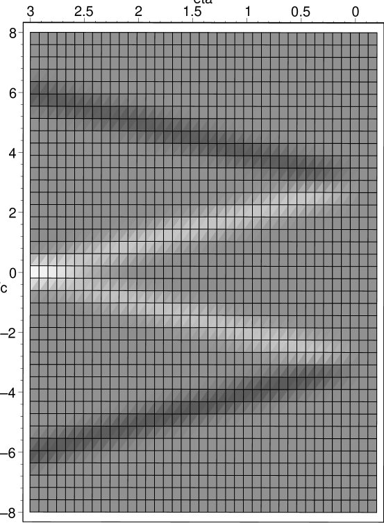
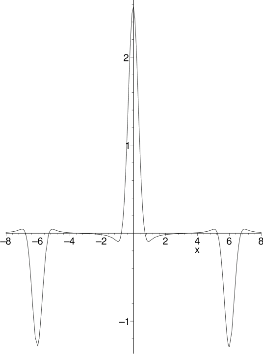
Figure 1: On the left, we have plotted $\Theta(\eta,{\bf x})$ of Eq. (29) in a 1 dimensional case. We have rescalled the spatial direction by $c_{s}$ the speed of the wave. The wave-packets have a mean momentum $c_{s}\bar{k}=\pi/3$, a spread $\sigma=3$ and a phase $\phi=0$. The chosen R-wave is centered on $x=0$ at $\eta_{0}=3$. Reheating is at $\eta_{r}=-10^{-2}$. (Hence one has $c_{s}\bar{k}\eta_{0}=\pi$, i.e. $\bar{k}$ corresponds to the first peak in the CMB if $\eta_{0}$ corresponds to the recombination.) The conformal time ranges from reheating to $\eta=\eta_{0}$. On the right, we present a spatial section at $\eta=\eta_{0}$.

IV.2 The Klein-Gordon product

When using the Klein-Gordon scalar product in the place of the simple product of Eq. (29), one gets

$$\Theta_{KG}({\bf x},\eta;\,{\cal V}_{R}) = \int\!\!{d^{3}x^{\prime}}\,G_{in}(\eta,{\bf x},\eta_{0},{\bf x}^{\prime})\,i\!\!\stackrel{{\scriptstyle\leftrightarrow}}{{\partial}}_{\eta_{0}}(\bar{\phi}_{R}^{(+)}(\eta_{0},{\bf x}^{\prime})-c.c.)=$$ (36)

$$= \int\!\!\widetilde{d^{3}k}\,\,n_{k}\,v_{\bf k}{\frac{e^{i{\bf k\bf x}}}{(2\pi)^{3/2}}}\,\left(\phi_{k}^{out}+z_{k}^{*}\phi_{k}^{out\,*}+c.c.\right)$$

$$= 2Re\left(i\partial_{\eta}\Psi_{{\cal V}_{R}}^{(+)}({\bf x}-{\bf x}_{0},\eta-\eta_{0})\right.$$

$$\quad\quad\quad\left.-i\partial_{\eta}\Psi_{{\cal V}_{R}}^{(+)}({\bf x}-{\bf x}_{0},-(\eta+\eta_{0}-4\eta_{r})\right)\,,$$

where the positive frequency wave $\Psi^{(+)}_{{\cal V}_{R}}$ is defined in Eq. (32). On the first line, we have used the difference between the positive and negative frequency components of $\bar{\phi}_{R}$ in order to cancel the minus sign which appears in the Klein Gordon product. On the second line we thus get the real part of the integrand. It differs from that of Eqs. (31,32) in two respects. First there is an extra factor of $k$ which arises from the derivative with respect to $\eta$. Second and more importantly, the KG product of wave with opposite frequencies (i.e. velocities for a given $\bf k$) vanishes. Hence this leads to a reduction of the four contributions of Eq. (31) to two waves forming a single pair.

When using the KG product between the two-point function $G_{in}$ and a $R$-moving wave, one thus correctly isolates the pair whose $R$-moving mode corresponds to the chosen wave. Together with Eq. (31), this is the main result of this Section.

The extraction of the contribution of a single pair is clearly displayed in Figure 2. The two wave packets originate near the reheating from a small patch which is centered at $({\bf x}_{R}+{\bf x}_{L})/2$. In fact the two waves travel on the would be particle horizon, i.e. the particle horizon if there were no inflation before $\eta_{r}$. This can be seen from the fact that the solution of ${\bf x}_{R}-{\bf x}_{L}=0$, i.e. the tip of the lightcone, gives $\eta=-2\eta_{r}$ which would correspond to $a=0$. The spatial extention of the patch at the reheating is governed by the spread of the waves: $1/\sigma$. From these results, one finds that in a radiation dominated era, the partner of a gravitational wave is always outside the Hubble radius centered on the other wave. This means that the coherence will never be detectable by any measurement performed within a Hubble radius. (In this one gets a situation similar to that of Hawking radiation since the partners of Hawking quanta are all inside the horizonPhysRep95 ). However, thanks to the imprint they leave on the LSS, both members can now be seen by us (when they are properly aligned, see Figure 3).

As previously discussed, the two waves are in phase opposition. Moreover, because of scale invariance, the above properties are valid for all wave packets.

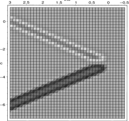
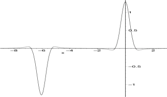
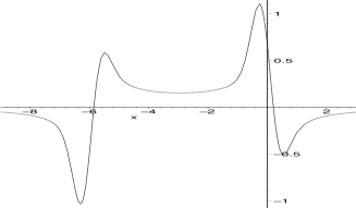
Figure 2: On the left, we have plotted $\Theta_{KG}$ in conformal coordinates. The conventions are identical to those of Figure 1. On the right we have presented sections at $\eta=\eta_{0}=3$ of this amplitude for two different choices of the phase $\phi$: $\phi=0,\,\pi/3$. In each case, the partner wave is in phase opposition in the sense that Eq. (66). The two waves are separated by $2(\eta_{0}-2\eta_{r})\simeq 6$. This filtering giving rise to the contribution of a single pair will be recovered in Section VI by performing a projection in configuration space rather than a product in space-time as in Eq. (36).

IV.3 Spreads

It is of great interest to analyze the spreads of the various contributions in Eq. (33) or Eq. (36). Indeed their properties can be exploited to reveal the presence of the correlations between $R$ and $L$ sectors.

The result of the saddle-point evaluation of Eq. (32) is given by, see CP1 :

$$\Phi_{{\cal V}_{R}}({\bf x})\sim Re\left[\frac{1}{\sqrt{{\rm{det}\Sigma|_{\bar{\bf k}}}}}e^{\chi({\bf\bar{k}})}\exp\left(-\frac{1}{2}{\bf x}_{i}(\Sigma^{-1})_{ij}{\bf x}_{j}\right)\right]\,,$$ (37)

where the function $\chi({\bf k})$ regroups the terms in the exponential of the integrand in Eq. (32). The matrix $\Sigma$ is defined by $2\Sigma_{ij}=-\partial_{i}\partial_{j}\chi|_{{\bf\bar{k}}}$ where $i,j=1,2,3$ label the three conformal coordinates. The three eigenvalues of $\Sigma_{ij}$ give the spreads in position of the Gaussian wave-packet Eq. (37). In the case of a single wave-packet with axial symmetry around $\bf\bar{k}$, the three eigenvalues reduce to two scalars. The first one is the spread in direction longitudinal to $\bf\bar{k}$. It is independent of time and equal to $1/|\sigma|$, as in one dimension. The other governs the spread in the directions orthogonal to $\bf\bar{k}$. It grows linearly with time, as in the case of a non-relativistic wave-packet. Its value therefore differs for the $R$ and $L$ wave:

$$2\Sigma_{\bot,\,R}^{2}(\eta) = \frac{1}{2\sigma^{2}}+i\frac{\eta-\eta_{0}}{\bar{k}}\,,$$ (38)

$$2\Sigma_{\bot,\,L}^{2}(\eta) = \frac{1}{2\sigma^{2}}+i\frac{\eta+\eta_{0}-4\eta_{r}}{\bar{k}}\,.$$ (39)

When $\sigma$ is taken real, the spread of the R-wave is minimal at $\eta=\eta_{0}$, as expected. (Remember that the spread in the perpendicular directions is given by the square root of the norm of $\Sigma$). The spread of the partner L-wave is thus larger as it is governed by the accumulated conformal time from the detection of the R wave at $\eta_{0}$, back to $\eta_{r}$ where the pair emerges, and then forward to $\eta_{0}$, for more details see CP1 . The relative increase of L-wave spread becomes large for short wave lengths modes. As an example, for a wave-packet of mean momentum $\bar{k}(\eta_{0}-2\eta_{r})=10$ (this would correspond to the third peak in the CMB anisotropies spectrum) and spread $\sigma=\bar{k}$, one has $|\Sigma_{L}(\eta_{0})/\Sigma_{R}(\eta_{0})|\simeq 6$.

It is now crucial to notice that one can fine tune the imaginary part of $\sigma$ to obtain a partner wave which is more peaked than the wave which is chosen in Eq. (29). Indeed, one can exploit the coherence of the wave packet and that of the vacuum, i.e. the ${\bf k}$ dependence of Eqs. (42, 84), to obtain constructive interferences around ${\bf x}_{L}$ by canceling the accumulated effect due to the total time of flight. The maximal effect, i.e. the minimal norm of $\Sigma_{L}(\eta_{0})$, is reached when taking $Im(\sigma^{-2})=-4(\eta_{0}-2\eta_{r})/\bar{k}$. When considering the above example with $\bar{k}(\eta_{0}-2\eta_{r})=10$, one gets

$$\mbox{$|{\Sigma_{L}(\eta_{0})}/{\Sigma_{R}(\eta_{0})}|$}\simeq\frac{1}{6}\,,$$ (41)

that is, the perpendicular spread in space of the partner wave is about six times smaller than that of the wave which is used in the integration of Eq. (36). This reduction of the partner wave spread is a direct consequence of the two-mode $R-L$ coherence. Hence it can be used as a check to quantify the degree of coherence given some observational data. It should be also noticed that it is not necessary to identify the velocity in order to bring this effect into evidence. Indeed this reduction equally applies to the spreads of the last two waves in Eq. (31). (In that case, the above symbols $R$ and $L$ should be interpreted in their generalized sense given after Eq. (33).)

In the next Sections, we present a more sophisticated procedure to extract space-time correlations. It is based on the introduction of a filter in configuration space before computing expectation values. Being not based on mean values, it allows to generalyse the former analysis. In particular it reveals correlations in the amplitude of wave packets. The reader not interested by these developments can proceed directly to the Conclusions where he will find a resume of the results.

V Coherent states, classical waves and random processes

We introduce coherent states of the field $\phi$. They are the key elements for our analysis of the correlations associated with a realization of a particular set of classical configurations. In quantum terms such a realization can be described by the detection of the corresponding states, namely coherent states. Moreover, since we want to select localized waves, we need to form wave packets by summing different $\mathbb{k}$-modes. Therefore, we shall work with coherent states of these wave packets.

The filtering of a set of classical waves is implemented by introducing a projector on the corresponding coherent state. The introduction of this projector modifies the correlations which existed in the “in vacuum”, i.e. the state of the system which encodes the pair creation process. New correlations are introduced at the expense of reducing the pre-existing ones. In particular spatial correlations are generated by detecting a local wave.

V.1 EPR correlations and conditional values

To describe the correlations which exist in the in vacuum, we analyze correlations amongst out states. To justify this analysis in the present context, let’s consider the following gedanken experiment. Suppose that $n$ $R$-out-particles of momentum $\mathbb{k}$ have been detected and that nothing is known for the other modes except that, before this detection, the field was in the in vacuum. Given that detection, one can ask what are the probabilities to find $m$ particles of momentum $\mathbb{k}^{\prime}$. The answers to this type of questions are governed by the partially ‘reduced’ state obtained by projecting the in vacuum onto the state characterizing the (partial) detection, namely $|n,\,\mathbb{k},R,out\rangle$:

$$|{\rm red}_{n,\,\mathbb{k},R}\rangle=\langle n,\,\mathbb{k},R,out|0,in\rangle_{2}=\frac{(z_{k})^{n}}{|\alpha_{k}|}\,\mbox{$|n,\,\mathbb{k},L,out\rangle$}\widetilde{\prod\limits_{\mathbb{k}^{\prime}\neq\mathbb{k}}}\otimes|0,\,\mathbb{k}^{\prime},in\rangle_{2}\,.$$ (42)

In the $\mathbb{k}$-th two-mode sector, one finds the one-mode $L$-state entangled to $|n,\,\mathbb{k},R,out\rangle$. It is a pure state with the same occupation number. This results from the EPR-type correlations present in the in vacuum, see Eq. (14). (These correlations deserve the label ‘EPR’ since they are of the same character as those encountered with spins: the spin projection on a axis is here replaced by the occupation number. Notice also that in both cases, a symmetry is at the origin of the entanglement, rotation invariance there, translation invariance here.) The two-mode sectors with $\mathbb{k}^{\prime}\neq\mathbb{k}$ are all unaffected by the detection. Therefore the probabilities to find particles of momentum $\mathbb{k}^{\prime}\neq\mathbb{k}$ are unchanged.

More generally, according to the rules of quantum mechanics, the “conditional” expectation values which result from the above detection can be written as

$$\langle\hat{\cal O}\rangle_{cond}=\frac{\langle\hat{\Pi}\,\hat{\cal O}\,\hat{\Pi}\rangle_{\rm in}}{\langle\hat{\Pi}\rangle_{\rm in}}\,,$$ (43)

where the projector onto the detected state $|n,\,\mathbb{k},R,out\rangle$ is

$$\hat{\Pi}_{{n,\,\mathbb{k},R,out}}=\mbox{$|n,\,\mathbb{k},R,out\rangle$}\langle n,\,\mathbb{k},R,out|\otimes{\mathbb{1}}_{\mathbb{k},L}\otimes{\mathbb{1}}_{\mathbb{k}^{\prime}\neq\mathbb{k}}\,.$$ (44)

In Eq. (43) we have used $\hat{\Pi}^{2}=\hat{\Pi}$ to simplify the denominator. The above projector is “partial” in that it is unity in all sectors but the $R$-mode $\mathbb{k}$.

The use of projectors which act only on the $R$ sector is particularly interesting because it guarantees that the $L$-mode content will be only determined by the correlations which are present in the state of the field. It is therefore the appropriate tool to unravel the intrinsic properties of the $R-L$ correlations. The next step is to determine how these correlations give rise to the spatial properties of conditional values. This is done in Sections VI. Notice finally that we shall no longer use projectors which specify the occupation number as in Eq. (44). Instead we shall use projectors based on coherent states because these properly characterize the various realizations of the ensemble, see footnote 3.

V.2 Coherent states and classical waves

Because of the entanglement between $R$ and $L$ modes in the in vacuum, only half of the modes are independent. Hence we shall use coherent states which are defined in the right sector only. We also work with out modes because the detection of waves is performed at late time, i.e. during the radiation or the matter dominated epoch. In this Section, we consider coherent states which specify the amplitudes of all $R$-modes:

$$\mbox{$|{\cal V},R\rangle$}=\widetilde{\prod\limits_{\bf k}}\otimes\mbox{$|v_{\bf k},R\rangle$}\,,$$ (45)

where $|v_{\bf k},R\rangle$ is a (one-mode) coherent state of complex amplitude $v_{\bf k}$, see Appendix B.

The product $|{\cal V},R\rangle$ is an eigenstate of $\hat{\phi}_{R}^{(+)}$, the right-moving positive frequency part of the field operator :

$$\hat{\phi}_{R}^{(+)}\mbox{$|{\cal V},R\rangle$} = \int\!\!\widetilde{d^{3}k}\,\frac{e^{i\mathbb{k}\mathbb{x}}}{(2\pi)^{3/2}}\phi_{k}^{out}(\eta)\,\hat{a}_{\mathbb{k}}^{out}\mbox{$|{\cal V},R\rangle$}$$ (46)

$$= \int\!\!\widetilde{d^{3}k}\,\frac{e^{i\mathbb{k}\mathbb{x}}}{(2\pi)^{3/2}}\phi_{k}^{out}(\eta)v_{\mathbb{k}}\mbox{$|{\cal V},R\rangle$}$$

$$= \bar{\phi}_{R}^{(+)}\,\mbox{$|{\cal V},R\rangle$}\,.$$

where the tilde on $d^{3}k$ means that one integrates over $R$ modes only, i.e. $k_{x}$ is integrated from $0$ to $\infty$. The function $\bar{\phi}_{R}^{(+)}$ is complex because it contains only positive frequencies. To get a real function, one should consider the expectation value of the observable $\hat{\phi}_{R}$, the field amplitude itself:

$$\bar{\phi}_{R}=\mbox{$\langle{\cal V},R|$}\hat{\phi}_{R}\mbox{$|{\cal V},R\rangle$}=\mbox{$\langle{\cal V},R|$}(\hat{\phi}_{R}^{(+)}+\hat{\phi}_{R}^{(-)})\mbox{$|{\cal V},R\rangle$}=2Re\left\{\bar{\phi}_{R}^{(+)}\right\}\,.$$ (47)

The same can be done to the conjugate momentum of the field, see Eq. (B).

We can now verify that the (dominant part of the) expectation values computed in the state $|{\cal V},R\rangle$ can be expressed directly in terms of the mean value $\bar{\phi}_{R}$, in the same way that Eq. (20) was expressed in terms of the two sine functions.

Using the normalisation of Eq. (24), the amplitude $\bar{v}$ is related to the expectation value of the occupation number

$$\mbox{$\langle{\cal V},R|$}\hat{N}_{R}\mbox{$|{\cal V},R\rangle$}=\int\!\!\widetilde{d^{3}k}\,\mbox{$\langle{\cal V},R|$}\hat{a}_{\bf k}^{R\,\dagger}\hat{a}^{R}_{\bf k}\mbox{$|{\cal V},R\rangle$}=\bar{v}^{2}\,.$$ (48)

It is also related to the current of $\bar{\phi}_{R}^{(+)}$:

$$\int\!\!d^{3}x\,\,\bar{\phi}_{R}^{(-)}\,i\!\!\stackrel{{\scriptstyle\leftrightarrow}}{{\partial_{\eta}}}\bar{\phi}_{R}^{(+)}=\bar{v}^{2}\,.$$ (49)

Thus one has two alternative descriptions. Either one uses the quantum description in terms of the expectation value based on the counting operator or the classical concept of current based on the mean wave $\bar{\phi}_{R}^{(+)}$. The same conclusion is valid for other quantities such as Green functions, see Appendix B, or the 3-momentum. In all cases, when $\bar{v}^{2}\gg 1$, the classical expressions based of the mean field $\bar{\phi}_{R}$ coincide with the corresponding expectation values evaluated in the coherent state $|{\cal V},R\rangle$. The reason is that the ambiguities of operator ordering lead to differences governed by commutators which are subdominant in the large occupation number limit.

V.3 Detections and random processes

In this subsection we show two important results. First, when the (Heisenberg) state is the in-vacuum, the detection of the $R$-moving configurations $\bar{\phi}_{R}$ described by the coherent state $|{\cal V},R\rangle$ is a stochastic Gaussian process. This result is exact: it requires no approximation and is valid even before applying any decoherence process. Notice however that, because of the entanglement between the $R$ and $L$ sectors, the particle content of only half the modes (e.g. the $R$-moving configurations) should be specified to get this result. Second, the detection of $\bar{\phi}_{R}$ fixes the $L$ modes to be also described by coherent states. This result is also exact and follows from the Gaussianity of squeezed states and the $R-L$ entanglement. These two results entirely determine the correlations which result from the detection of semi-classical configurations described by coherent states.

To determine the consequences of a detection, it is appropriate to introduce the associated projector, see subsection V.1. In the present case, it is

$$\hat{\Pi}_{{\cal V}_{R}}=\mbox{$|{\cal V},R\rangle$}\mbox{$\langle{\cal V},R|$}\otimes\mathbb{1}_{L}\,.$$ (50)

It is non trivial in the $R$-sector only. The probability to detect the classical wave $\bar{\phi}_{R}$ is given by

$$P^{in}_{{\cal V}_{R}}=\mbox{$\langle 0\,in|$}\hat{\Pi}_{{\cal V}_{R}}\mbox{$|0\,in\rangle$}=\widetilde{\prod\limits_{\mathbb{k}}}\mbox{$|A^{in}_{\mathbb{k}}|$}^{2}\,,$$ (51)

where the amplitude for the $\mathbb{k}$-mode is

$$A^{in}_{\mathbb{k}} = \frac{1}{|\alpha_{k}|}e^{-\frac{|v_{\mathbb{k}}|^{2}}{2|\alpha_{k}|^{2}}}\,,$$ (52)

see Eq. (104) for the details. The probability Eq. (51) defines a normalized gaussian distribution for each $R$-mode in every two-mode sectors. The normalization follows from the “density” of coherent states, see Eq. (105). As already mentioned, only $R$-modes have been so far specified. Had we performed a projection on both right and left sectors, the probability would have been exponentially smaller. Indeed, the ratio of the probabilities with or without double projection is, see Eqs. (54) and (96),

$$\frac{P^{in}_{{\cal V}_{R}\,,{\cal W}_{L}}}{P^{in}_{{\cal V}_{R}}}=\widetilde{\prod\limits_{\mathbb{k}}}\exp\left(-|w_{\bf k}-z_{k}v_{\bf k}^{*}|^{2}\right)\,,$$ (53)

where $w_{\bf k}$ is the amplitude of the coherent wave in the $L$-sector.

This exponentially suppression results from the entanglement between the left and right sectors. Indeed, when applying the projector $\hat{\Pi}_{{\cal V}_{R}}$ on the in vacuum one gets

$$\hat{\Pi}_{{\cal V}_{R}}\mbox{$|0,in\rangle$} = \widetilde{\prod\limits_{\mathbb{k}}}\,A^{in}_{\mathbb{k}}\,\mbox{$|v_{\mathbb{k}},\,\mathbb{k},R\rangle$}\otimes\mbox{$|z_{\mathbb{k}}v_{\mathbb{k}}^{*},\,\mathbb{k},L\rangle$}\,.$$ (54)

It is remarkable that in each two-mode sector, the $L$-state is also a coherent state. This results from Eq. (42), see also Eq. (103). The $L$-mode amplitude is $z_{k}v_{\mathbb{k}}^{*}$. It is fixed by the $R$-amplitude $v_{\mathbb{k}}$ and by the pair creation process which is governed by $z_{k}$. The properties of the space time patterns we shall later exhibit directly follow from this double origin.

Taken together, Eqs. (51-54) show that the notion of stochastic processes naturally emerge when questioning the in vacuum by making use of coherent out states. More precisely we have the following. Firstly, as one might have expected, the $R$-mode amplitude $v_{\bf k}$ is a Gaussian stochastic variable of variance equal to $\mbox{$|\alpha_{k}|$}^{2}=n_{k}+1\simeq n_{k}$. Secondly, the ${\bf k}$-th $L$-mode amplitude is “slave driven” by the detection of the $R$-mode in that its probability is centered around $z_{k}v_{\mathbb{k}}^{*}$ with a spread equal to 1, see Eq. (53). Therefore, in the large $n_{k}$ limit, this spread is negligible and one can consider that the $L$-mode amplitude is equal to $z_{k}v_{\mathbb{k}}^{*}$. Thus, in the stochastic description as well, $P^{in}_{{\cal V}_{R}}$ is a two-mode distribution, as clearly seen from Eq. (54).

These properties offer an alternative way to express expectation values in the in vacuum. It suffices to apply the following substitution: first, at the level of amplitudes $\hat{a}^{R}_{\bf k}\to v_{\bf k}$, $\hat{a}^{L}_{\bf k}\to z_{k}v_{\mathbb{k}}^{*}$, and second at the level of the distributions, the quantum distribution $\hat{\rho}_{in}=\mbox{$|0in\rangle$}\mbox{$\langle 0in|$}$ should be replaced by $P^{in}_{{\cal V}_{R}}$ of Eq. (51). Notice that no dynamical assumption was needed, nor was it necessary to follow the time evolution of the modes.

The emergence of classicity rests on the high occupation number $n_{k}\gg 1$ and on the (restricted) set of questions formed by inquiring about the coherent out state content of the in vacuum. Even though these conclusions are not new GuthPi85 ; Matacz94 ; PolStar96 , the derivation which makes use of coherent states is particularly clear. In particular, it disentangles the question of the late time description of the in vacuum in the above stochastic terms from the more difficult question which concerns the evaluation of the time from which this stochastic description is valid. This time is determined by the efficiency of decoherence processes in the early cosmology, a subject not addressed in the present paper Hu97 ; KieferPol98 .

V.4 1-point and 2-point functions

Besides the above substitution, one can consider the projector $\hat{\Pi}_{{\cal V}_{R}}$ as in subsection V.1, namely as defining a new ensemble of configurations with modified expectation values given by Eq. (43). It is of interest to present these expectation values in some details. Starting with 1-point functions, we have

$$\langle\hat{a}_{\mathbb{k},\,R}^{out}\rangle_{{\cal V}_{R}}=v_{\mathbb{k}}\,,\quad\langle\hat{a}_{\mathbb{k},\,L}^{out}\rangle_{{\cal V}_{R}}=z_{k}v_{\mathbb{k}}^{*}\,.$$ (55)

In the in vacuum we had $\langle\hat{a}_{\mathbb{k},\,R}^{out}\rangle_{\rm in}=\langle\hat{a}_{\mathbb{k},\,L}^{out}\rangle_{\rm in}=0$. The interpretation of the modification is clear: once we know that the classical wave $\bar{\phi}_{R}$ has been detected, the mean $R$-amplitudes of the $R$ ${\mathbb{k}}$-modes are those of that wave. Moreover because of the EPR correlations in the in vacuum, the mean amplitudes of the associated $L$-modes are fixed by the detection of the $R$-wave $\bar{\phi}_{R}$ and $z_{k}$.

For the 2-point functions we have,

$$\langle\hat{a}_{\mathbb{k},\,R}^{\dagger\,out}\,\hat{a}_{\mathbb{k}^{\prime},\,R}^{out}\rangle_{{\cal V}_{R}}=v^{*}_{\mathbb{k}}v_{\mathbb{k}^{\prime}}\,,\qquad\langle\hat{a}_{\mathbb{k},\,L}^{\dagger\,out}\,\hat{a}_{\mathbb{k}^{\prime},\,L}^{out}\rangle_{{\cal V}_{R}}=z^{*}_{k}v_{\mathbb{k}}\,z_{k^{\prime}}v^{*}_{\mathbb{k}^{\prime}}\,,$$ (56)

$$\langle\hat{a}_{\mathbb{k},\,R}^{out}\,\hat{a}_{\mathbb{k}^{\prime},\,L}^{out}\rangle_{{\cal V}_{R}}=v_{\mathbb{k}}\,z_{k^{\prime}}v^{*}_{\mathbb{k}^{\prime}}\,,$$ (57)

$$\langle\hat{a}_{\mathbb{k},\,R}^{\dagger\,out}\,\hat{a}_{\mathbb{k}^{\prime},\,L}^{out}\rangle_{{\cal V}_{R}}=v^{*}_{\mathbb{k}}\,z_{k^{\prime}}v^{*}_{\mathbb{k}^{\prime}}\,.$$ (58)

In the first line, the main modification with respect to in vacuum correlations is the loss of the diagonal character in ${\mathbb{k}}$. This radical change follows from the strength of the projection induced by $\hat{\Pi}_{\cal V_{R}}$. Since all $R$-${\mathbb{k}}$ components are now described by coherent states, the above 2-point functions are entirely given by a disconnected contribution. For these 2-point functions, the correspondence mentioned in section IV.B is exact. However, this is not the case in general because of non-vanishing commutators (consider for instance $\langle\hat{a}_{\mathbb{k},\,R}^{out}\,\hat{a}_{\mathbb{k}^{\prime},\,R}^{\dagger\,out}\rangle_{{\cal V}_{R}}$). It is only in the large occupation number regime that the operator ordering gives subdominant corrections. In the second line, we see that the in vacuum correlations between $R$ and $L$ modes have been replaced by the “coherent state correlations” described by Eq. (54). They fix $\langle\hat{a}_{\mathbb{k},\,L}^{out}\rangle_{{\cal V}_{R}}$ in terms of $\langle\hat{a}_{\mathbb{k},\,R}^{out}\rangle_{{\cal V}_{R}}$. Notice finally that the variances of $\hat{a}^{out}_{\mathbb{k},\,R}$ and $\hat{a}_{\mathbb{k}^{\prime},\,L}^{out}$ vanish, see Eq. (89). The detection of a coherent state of the field can thus be seen as providing one classical realization of the stochastic ensemble.

Before examining the correlations in space induced by the detection of $\bar{\phi}_{R}$, it is of value to determine to what extend one recovers (in vacuum) mean values from these conditional expectation values and from the distribution $P^{in}_{{\cal V}_{R}}$. Using Eq. (53) and Eq. (52), one finds that the ensemble average is defined by

$$\langle\langle v_{\mathbb{k},\,R}\,w_{\mathbb{k}^{\prime},\,L}\rangle\rangle_{\rm{in}} = \frac{\int\!\!\widetilde{\cal D}v_{\bf p}\widetilde{\cal D}w_{\bf q}\,\,v_{\bf k}w_{\bf k^{\prime}}\,P^{in}_{{\cal V}_{R},\,{\cal W}_{L}}}{\int\!\!\widetilde{\cal D}\,v_{\bf p}\,\widetilde{\cal D}w_{\bf q}\,P^{in}_{{\cal V}_{R},\,{\cal W}_{L}}}$$ (60)

$$= \frac{\int\!\!\widetilde{\cal D}v_{\bf p}\,\,v_{\bf k}z_{k^{\prime}}v_{\bf k^{\prime}}^{*}\,P^{in}_{{\cal V}_{R}}}{\int\!\!\widetilde{\cal D}v_{\bf p}\,P^{in}_{{\cal V}_{R}}}=z_{k}\mbox{$|\alpha_{k}|$}^{2}\delta^{3}({\bf k}-{\bf k^{\prime}})\,.$$

The tilde over the functional integration is there to remind that the integration variables $v_{\bf k}$ ($w_{\bf k}$) are defined only for $k_{x}>0$, thus $\widetilde{\cal D}v_{\bf k}=\widetilde{\prod\limits_{\bf k}}dv_{\bf k}$. The result of Eq. (60) is in agreement with the quantum result Eq. (18). For the diagonal $R$ term, the correspondence between the ensemble average and the quantum result Eq. (17) is not exact and the mean values differ by a factor equal to $|z_{k}|^{2}$. The origin of this discrepancy is that the $\hat{a}^{\dagger}_{{\bf k},\,R}\hat{a}_{{\bf k^{\prime}},\,R}$ does not commute with the projector $\hat{\Pi}_{{\cal V}_{R}}$, see also the third footnote. However, since the discrepancy rests on commutators, the two versions will agree when $n_{k}\to\infty$. This agreement in the large occupation number limit confirms that field configurations are effectively characterized by a set of stochastic variables ${\cal V}$ with the two-mode probability distribution $P^{in}({\cal V})$.

VI Spatial correlations

In the preceding subsection we gave the new expectation values when having detected the classical right moving configuration $\bar{\phi}_{R}$. Here we shall see that this detection leads to specific correlations in space. To exhibit these correlations it suffices to compute the modified expectation value of the field amplitude:

$$\langle\hat{\phi}(\eta,{\bf x})\rangle_{{\cal V}_{R}}=\bar{\phi}_{R,\,{\cal V}_{R}}+\bar{\phi}_{L,\,{\cal V}_{R}}\,,$$ (61)

where the $R$ and $L$ mean waves are

$$\bar{\phi}_{R,\,{\cal V}_{R}}(\eta,{\bf x}) = \int\!\!\widetilde{d^{3}k}\,\left(v_{\mathbb{k}}\,\frac{e^{i\mathbb{k}\mathbb{x}}}{(2\pi)^{3/2}}\phi_{k}^{out}(\eta)+c.c.\right)\,,$$ (62)

$$\bar{\phi}_{L,\,{\cal V}_{R}}(\eta,{\bf x}) = \int\!\!\widetilde{d^{3}k}\,\left(z_{k}v_{\mathbb{k}}^{*}\,\,\frac{e^{-i\mathbb{k}\mathbb{x}}}{(2\pi)^{3/2}}\phi_{k}^{out}(\eta)+c.c.\right)\,.$$ (63)

Eq. (62a) should cause no surprise. Since the projector $\hat{\Pi}_{{\cal V}_{R}}$ completely specifies $R$-configurations, expectation values in the $R$ sector are given by the coherent state expectation values as in subsection IV.A. Eq. (62b) is more subtle as it arises both from this projector as well as from the EPR correlations, Eq. (54). Because of the latter, the mean value of the $L$-part of the field operator, $\hat{\phi}_{L}$, is also described by a local wave packet even though nothing has been specified about $L$-configurations.

The main lesson from these equations is that the simultaneous specification of the various $v_{\bf k}$ has introduced some spatial coherence by coupling modes which were so far independent. To obtain these spatial properties, we re-use the wave packet given in Eq. (25). The $R$-wave is then given by Eq. (27) which is maximum along the classical light-like trajectory of Eq. (28). More interesting is the partner wave, the $L$ component. Using Eq. (84), one has

$$\bar{\phi}_{L,\,{\cal V}_{R}}=-\,\bar{v}N\int\widetilde{d^{3}k}\frac{1}{\sqrt{2k}}e^{-\frac{(\bf k-\bar{\bf k})^{2}}{4\sigma^{2}}}\left(e^{-i\bf k(\bf x-\bf x_{0})}e^{-ik(\eta+\eta_{0}-4\eta_{r})}e^{-i\phi}+c.c\right)\,.$$ (65)

Two interesting properties should be discussed. First, using the stationary phase condition one determines the partner’s trajectory ${\bf x}_{L}$ defined in Eq. (34). As expected one verifies that the partner propagates in the opposite direction. More importantly, it is separated from the detected wave by the ‘universal’ distance given in Eq. (35). Secondly, the phases of the two waves are opposite when evaluated at the centers of the wave-packets, compare Eq. (27) and (65). This phase opposition is particularly clear when working in 1 dimension. In this case, for any right moving wave packet, one has

$$\bar{\phi}_{L,\,{\cal V}_{R}}({\bf x};\phi)=\bar{\phi}_{R,\,{\cal V}_{R}}({\bf x}-{\bf x}_{R}+{\bf x}_{L};\phi+\pi)\,.$$ (66)

In Section IV, we have seen that a similar result obtains in 3 dimensions when working at the saddle-point approximation. This phase opposition originates from the coherence in the in-vacuum, see Eq. (14) and Eq. (84). (Notice that it also follows from the neglect of the decaying mode). It has important physical consequences. It implies that the partner of a local Newton (Bardeen) potential dip is a local hill. For adiabatic perturbations, it means that the partner of a hot region is a cold region. It is to be emphasized that these correlations are valid for every configurations specified by Eq. (45) and not only in the mean.

In brief, by having isolated from the in vacuum the $(\bar{\bf k},\bar{v})$ $R$ configuration centered around ${\bf x_{0}}$ at $\eta_{0}$, we obtain a causally disconnected $L$ configuration which is centered around ${\bf x}_{0}-2(\eta_{0}-2\eta_{r})\,{\bf 1}_{\bar{\bf k}}$, has momentum $-\bar{\bf k}$, and which has the same amplitude $\bar{v}$ and opposite phase. Notice that these results follow from the fact that $\langle\hat{\phi}\rangle_{{\cal V}_{R}}$ given in Eq. (61) is in fact a single wave packet of in modes. Notice finally that we have reached these results by making use of the complete projector $\hat{\Pi}_{{\cal V}_{R}}$ which specified the amplitudes of all $R$-modes. However these results can also be obtained when performing only a partial selection which leaves unspecified the amplitudes of all $R$-wave packets orthogonal to the chosen one. The proof is given in the Appendix D. It rest on the Gaussianity of the distribution.

VII Conclusions and Discussions

In the second part of this paper we have shown the following results. When considering (long after the reheating) the set of final configurations of a quantum field in an inflationary model, the detection of a coherent state describing half the modes (e.g. a right moving configuration) is a random process, see Eq. (51). Second, the fact that modes have been amplified in pairs implies that the “reduced state” which follows from this detection is also a coherent state, see Eq. (54). Therefore, when specifying that some local waves have been detected, one introduces spatial correlations which possess definite properties. In particular these correlations always have the same dipolar structure since the amplification process is scale invariant. Moreover, the two waves in each pair are in phase opposition because of Eq. (84) which tells us that the linear $k$ dependence of the phase of $z_{k}$ will only induce a translation of the partner’s wave with respect to the chosen one. Indeed, this linear dependence implies that the separation between the two waves is always given by twice the Hubble time multiplied by the speed of the waves, in a direction specified by their wave vector, see Eq. (34). The phase opposition means that the spatial profile of the partner wave is the symmetrical of that of the chosen wave, see Eq. (66), up to a question of the spreads in the perpendicular directions, see Eqs. (38). It should be also pointed out that there also exists a strict correlation in the amplitudes of the two waves in each pair. This correlation in amplitude cannot be seen from the simpler treatment based on the two-point function since the mean has been taken before having applied the wave packet transformation. In addition to this discrepancy, when using a product which is insensitive to the sign of the wave velocity, as in Eq. (29), we obtain the three folded structure since the contribution of two pairs are isolated by computing the spatial overlap, see Figure 1.

One might finally question if it would be possible to observe these structures. Let us briefly mention the different aspects which should be confronted.

One should first analyze the statistical basis for the identification. We first notice that Eq. (31) results from having taken an ensemble average (which could be thought to be either quantum or stochastic). This mean value could be reached observationally if a sufficiently large number of (independent) pairs are considered. In this, one should exploit the isotropy and the homogeneity of the distribution, as for the temperature anisotropy multipoles. When dealing with modes with sufficiently high wave vectors (corresponding to angles smaller than a degree), this condition can probably be met.

Second, we have access only to a portion of the configurations at recombination time, namely the Last Scattering Surface ${\cal{S}}$, the intersection of $\eta=\eta_{rec}$ with our past light cone, see Fig. 3. Since all pairs propagate on the particle horizon of the locus of birth, at recombination, they fall into three classes. First there exist pairs which do not intercept the LSS, such as the pair $1$. These do not contribute at all to the temperature anisotropies. Second there exist pairs such as $2$ for which only one member crosses the LSS. These contribute incoherently (i.e. as if $c_{k}=0$) to the temperature anisotropies. Third one finds the pairs such that both members live on the LSS. They contribute coherently to the anisotropies. Hence only these are responsible for the dip in the function $C(\theta)$ mentioned in BB . These pairs have their wave vector tangent to ${\cal{S}}$. Their number is therefore limited by these geometrical constraints. To quantify the percentage of such pairs, one must consider the depth of the LSS. These aspects will be presented in a forthcoming publication.

Moreover, the temperature anisotropies do not arise solely from the density fluctuations on the LSS. For a description of the various contributions, we refer to priorM ; Mukhanov03 . Notice that the Doppler effect does not affect the temperature fluctuations which propagate longitudinally with respect to the LSS. Instead the contribution of secondary anisotropies will lower the level of coherence of temperature anisotropies.

Finally, would be very interesting to have access to the velocity field on the LSS in order to be able to suppress the doubling of the partners. Maybe a clever use of the polarization spectra might allow to reconstruct this field. Before trying to do so one might first look for a statistical identification of three folded structure. We re-emphasize the statistical character of this structure which results from an averaging procedure over pair creation events which individually form local dipoles.

Figure 3: A $2+1$ dimensional space-time diagram in conformal coordinates $(\eta,x,y)$. The Last Scattering Surface ${\cal{S}}$ is here represented by a circle defined by the intersection of our past light-cone ${\cal{C}^{-}}$ with the 2d-spacelike surface $z=cte,\eta=\eta_{LSS}$. All pairs are created at reheating $\eta_{reh}$ and propagate on light-cones. Given that the recombination is almost instantaneous, only few pairs, such as $3$, are such that both particles intercept ${\cal{S}}$.

${\bf{Acknowledgements}}$
We would like to thank Ted Jacobson, Serge Massar, Simon Prunet, and Jean-Philippe Uzan for useful remarks.

Appendix A The Bogoliubov transformation from inflation to the adiabatic era

Since we use quantum settings, we need the Bogoliubov coefficients relating positive frequency modes during inflation (taken here to be for simplicity a de Sitter period) to modes during the radiation and matter dominated eras.

In these three periods, the scale factor is given by

$$a(\eta) = -\frac{1}{H\eta}\,,\qquad{\mbox{for\, \, }}-\infty<\eta<\eta_{r}<0\,,$$ (67)

$$a(\eta) = \frac{1}{H\eta_{r}^{2}}(\eta-2\eta_{r})\,,\qquad{\mbox{for\, \, }}\eta_{r}<\eta<\eta_{eq}\,,$$ (68)

$$a(\eta) = \frac{1}{4H\eta_{r}^{2}}\frac{(\eta-4\eta_{r}+\eta_{eq})^{2}}{\eta_{eq}-2\eta_{r}}\,,\qquad{\mbox{for\, \, }}\eta_{eq}<\eta\,,$$ (69)

where $\eta_{r}$ and $\eta_{eq}$ designate respectively the end of inflation and the time of equilibrium between radiation and matter. The shifts in the parenthesis in the second and third lines are necessary to parametrize the three periods by a single conformal time $\eta$. The sudden pasting of these periods are such that the scale factor and the Hubble parameter are continuous functions.

The positive-frequency solutions of Eq. (4) (corresponding to gravitational waves, the modes for density fluctuations having a different dispersion relation, see the second footnote) are

$$\phi_{k}^{in}(\eta) = \frac{1}{\sqrt{2k}}\left(1-\frac{i}{k\eta}\right)e^{-ik\eta}\,,\quad\mbox{for\, \,}-\infty<\eta<\eta_{r}\,,$$ (71)

$$\phi_{k}^{rad}(\eta) = \frac{1}{\sqrt{2k}}e^{-ik\eta}\,,\quad\mbox{for\, \, }\eta_{r}<\eta<\eta_{eq}\,,$$ (72)

$$\phi_{k}^{mat}(\eta) = \frac{1}{\sqrt{2k}}\left(1-\frac{i}{k(\eta-\eta_{m})}\right)e^{-ik\eta}\,,\quad\mbox{for\, \,}\eta_{eq}<\eta\,,$$ (73)

where we note $\eta_{m}=4\eta_{r}-\eta_{eq}$. The Bogoliubov coefficients between these modes are

$$\phi_{k}^{in}(\eta) = \alpha_{k}^{in-rad}\ \phi_{k}^{rad}(\eta)+\beta_{k}^{in-rad\,*}\ \phi_{k}^{rad\,*}(\eta)\,,$$ (75)

$$\phi_{k}^{rad}(\eta) = \alpha_{k}^{rad-mat}\ \phi_{k}^{mat}(\eta)+\beta_{k}^{rad-mat\,*}\ \phi_{k}^{mat\,*}(\eta)\,.$$ (76)

The coefficients $\alpha_{k}$ and $\beta_{k}$ of the first line are given by the Wronskians

$$\alpha_{k}^{in-rad}=\left(\phi_{k}^{R},\phi_{k}^{in}\right)\mbox{, \ \ }\beta_{k}^{in-rad\,*}=-\left(\phi_{k}^{R\,*},\phi_{k}^{in}\right)\,,$$ (78)

evaluated at transition time $\eta_{r}$ since modes satisfy different equations in each era. Similar expressions evaluated at the equilibrium time $\eta_{eq}$ hold for the coefficients between $\phi^{rad}_{k}$ and $\phi^{mat}_{k}$. One gets

$$\alpha_{k}^{in-rad} = 1-\frac{i}{k\eta_{r}}-\frac{1}{2k^{2}\eta_{r}^{2}}\,,$$ (79)

$$\left(\beta_{k}^{in-R}\right)^{*} = \frac{e^{-2ik\eta_{r}}}{2k^{2}\eta_{r}^{2}}\,,$$ (80)

$$\alpha_{k}^{rad-mat} = 1+\frac{i}{k(\eta_{eq}-\eta_{m})}-\frac{1}{2k^{2}(\eta_{eq}-\eta_{m})^{2}}\,,$$ (81)

$$\left(\beta_{k}^{rad-mat}\right)^{*} = \frac{-e^{-2ik\eta_{eq}}}{2k^{2}(\eta_{eq}-\eta_{m})^{2}}\,.$$ (82)

These Bogoliubov coefficients have been calculated for gravitational waves in Allen88 ; Allen94 . Their results agree with ours up to constant phases which can be gauged away by a mode redefinition. For density fluctuations similar expressions are obtained when using the appropriate frequency.

For relevant modes, i.e. modes which contribute to visible anisotropies in the CMB, their wave length obeys $k/Ha(\eta_{r})=k|\eta_{r}|\ll 1$. In the limiting case, to order $(k\mbox{$|\eta_{r}|$})^{3}$, one has

$$\beta_{k}/\alpha_{k}^{*}=z_{k}=-e^{4ik\eta_{r}}\,.$$ (84)

Thus the in modes during the radiation dominated era read

$$\phi_{k}^{in}(\eta) = \frac{i}{\sqrt{2}k^{3/2}\eta_{r}^{2}}\left(\frac{\sin(k(\eta-2\eta_{r}))}{k}+O((k\eta_{r})^{3})\right)\,,\qquad\eta\gg\eta_{r}\,.$$ (85)

One then verifies that the physical modes $\xi_{k}=\phi_{k}^{in}/a$ are constant (and $=H/(2k^{3/2})$ until they re-enter the Hubble radius, i.e. when $k(\eta-2\eta_{r})$ approaches $1$. This guarantees a scale invariant spectrum $k^{3}\mbox{$|\xi_{k}|$}^{2}=H^{2}$ Finally, since $\xi_{k}$ is constant the approximation which consists in dropping terms of $O((k\eta_{r})^{3})$ in Eq. (85) corresponds to the neglect of the decaying mode, see the discussion after Eq. ((20)).

Appendix B Coherent states for a real harmonic oscillator

This appendix aims to give a self-contained presentation of coherent states, with special emphasis on properties which shall be used in the body of the manuscript. For more details, we refer to Glauber63a ; Glauber63b ; Zhang90 .

They are several equivalent ways to define coherent states. The definition we adopt Glauber63b is as an eigenstate of the annihilation operator:

$$\hat{a}\mbox{$|v\rangle$}=v\mbox{$|v\rangle$}\,,$$ (86)

where $v$ is a complex number. The development on this state on Fock basis is

$$\mbox{$|v\rangle$}=e^{-\frac{|v|^{2}}{2}}\sum_{n=0}^{\infty}\frac{v^{n}}{\sqrt{n!}}\mbox{$|n\rangle$}\,,$$ (87)

where the exponential prefactor guarantees that the state is normalized to unity $\langle v|v\rangle=1$.

The first interesting property of coherent states is that they correspond to states with a well defined complex amplitude $v$. Indeed, by definition (86), the expectation values of the annihilation and creation operators are

$$\mbox{$\langle v|$}\hat{a}\mbox{$|v\rangle$}=v\,,\quad\mbox{$\langle v|$}\hat{a}^{\dagger}\mbox{$|v\rangle$}=v^{*}\,.$$ (88)

It is to be stressed that the variances vanish:

$$\Delta\hat{a}^{2}=\mbox{$\langle v|$}\hat{a}^{2}\mbox{$|v\rangle$}-\mbox{$\langle v|$}\hat{a}\mbox{$|v\rangle$}^{2}=0\,,\quad\Delta\hat{a}^{\dagger\,2}=\mbox{$\langle v|$}\hat{a}^{\dagger\,2}\mbox{$|v\rangle$}-\mbox{$\langle v|$}\hat{a}^{\dagger}\mbox{$|v\rangle$}^{2}=0\,.$$ (89)

Moreover the mean occupation number is

$$\mbox{$\langle v|$}\hat{a}^{\dagger}\hat{a}\mbox{$|v\rangle$}=\mbox{$|v|$}^{2}\,,$$ (90)

in agreement with the mean value given by the Poisson distribution (87).

¿From these properties one sees that the expectation values of the position and momentum operators (in the Heisenberg picture, with $\hbar=1$)

$$\hat{q}(t)=\frac{\hat{a}e^{-i\omega t}+\hat{a}^{\dagger}e^{i\omega t}}{\sqrt{2\omega}}\,,\qquad\hat{p}(t)=-i\sqrt{\frac{\omega}{2}}(\hat{a}e^{-i\omega t}-\hat{a}^{\dagger}e^{i\omega t})\,,$$

are

$$\bar{q}(t) = \mbox{$\langle v|$}\hat{q}(t)\mbox{$|v\rangle$}=\frac{1}{\sqrt{2\omega}}(ve^{-i\omega t}+v^{*}e^{i\omega t})=\sqrt{\frac{2}{\omega}}\mbox{$|v|$}\cos(\omega t-\phi_{v})\,,$$

$$\bar{p}(t) = \mbox{$\langle v|$}\hat{p}(t)\mbox{$|v\rangle$}=-i\sqrt{\frac{\omega}{2}}(ve^{-i\omega t}-v^{*}e^{i\omega t})=-\sqrt{2\omega}\mbox{$|v|$}\sin(\omega t-\phi_{v})=\partial_{t}\bar{q}(t)\,.$$ (91)

We have used the polar decomposition $v=\mbox{$|v|$}e^{i\phi_{v}}$. These expectation values have a well defined amplitude and phase and follow a classical trajectory of the oscillator. This is due to the “stability” of coherent states which is better seen in the Schödinger picture. If the state is a coherent state $|v\rangle$ at a time $t_{0}$, one immediately gets from (87) that at a later time $t$, the state is a coherent state given by $\mbox{$|v(t)\rangle$}=\mbox{$|ve^{-i\omega(t-t_{0})}\rangle$}$. Notice that the variances of the position and the momentum are

$$\Delta\hat{q}^{2}=\frac{1}{2\omega}\,,\qquad\Delta\hat{p}^{2}=\frac{\omega}{2}\,.$$ (92)

They minimize the Heisenberg uncertainty relations and are time-independent. Hence, in the phase space $(q,p)$, a coherent state can be considered as a unit quantum cell $2\pi\hbar$ in physical units (see also (105) for the measure of integration over phase space) centered on the classical position and momentum of the harmonic oscillator $(\bar{q}(t),\bar{p}(t))$. In the large occupation number limit $\mbox{$|v|$}\gg 1$, coherent states can therefore be interpreted as classical states since $\Delta\hat{q}/\bar{q}=\Delta\hat{p}/\bar{p}\propto 1/\mbox{$|v|$}$. This is a special application of the fact that coherent states can in general be used to define the classical limit of a quantum theory, see Zhang90 and references therein.

One advantage of coherent states Glauber63a is that the calculations of Green functions resembles closely to those of the corresponding classical theory (i.e. treating the fields not as operators but as c-numbers) provided either one uses normal ordering, or one considers only the dominant contribution when $\mbox{$|v|$}\gg 1$. In preparation for the calculations with field we compute the Wightman function in the coherent state $|v\rangle$

$$\widetilde{G}_{v}(t,t^{\prime}) = \mbox{$\langle v|$}\hat{q}(t)\hat{q}(t^{\prime})\mbox{$|v\rangle$}$$ (93)

$$= \langle:\hat{q}(t)\hat{q}(t^{\prime}):\rangle_{v}+\frac{1}{2\omega}e^{i\omega(t-t^{\prime})}$$

where we have isolated the contribution of the vacuum. The normal ordered correlator is order $\mbox{$|v|$}^{2}$:

$$\langle:\hat{q}(t)\hat{q}(t^{\prime}):\rangle_{v} = \frac{1}{\omega}\,Re\left[\langle\hat{a}^{2}\rangle_{v}e^{-i\omega(t+t^{\prime})}+\langle\hat{a}^{\dagger}\hat{a}\rangle_{v}e^{i\omega(t-t^{\prime})}\right]$$ (94)

$$= \frac{2}{\omega}|v|^{2}\cos(\omega t-\phi_{v})\cos(\omega t^{\prime}-\phi_{v})=\bar{q}(t)\,\bar{q}(t^{\prime})\,.$$

We see that the perfect coherence of the state, namely $\mbox{$|\langle\hat{a}\hat{a}\rangle_{v}|$}=\langle\hat{a}^{\dagger}\hat{a}\rangle_{v}$ is necessary to combine the contributions of the diagonal and the interfering term so as to bring the time-dependent classical position $\bar{q}(t)$ in Eq. (94).

The wave-function of a coherent state in the coordinate representation is given by

$$\psi_{v}(q)=\left(\frac{\omega}{\pi}\right)^{1/4}e^{-\frac{\omega}{2}(q-\bar{q})^{2}}e^{i\bar{p}q}\,,$$ (95)

where $v=(\bar{q}+i\bar{p})/\sqrt{2\omega}$. This follows from the definition $\mbox{$\langle q|$}\hat{a}\mbox{$|v\rangle$}=v\langle q|v\rangle$. ¿From this equation one notes that two coherent states are not orthogonal. The overlap between two coherent states is

$$\langle v|w\rangle=\exp\left(v^{*}w-\frac{1}{2}\mbox{$|v|$}^{2}-\frac{1}{2}\mbox{$|w|$}^{2}\right)\,.$$ (96)

Nevertheless they form an (over)complete basis of the Hilbert space in that the identity operator in the coherent state representation $\{\mbox{$|v\rangle$}\}$ reads

$${\bf 1}=\int\!\!\frac{d^{2}v}{\pi}\,\mbox{$|v\rangle$}\mbox{$\langle v|$}\,.$$ (97)

The measure is $d^{2}v=d(Rev)d(Imv)$. (This identity can be established by calculating the matrix elements of both sides of the equality in the coordinate representation $\{\mbox{$|q\rangle$}\}$, with the help of (95).)

Appendix C Two-mode squeezed states and coherent states

Since one can view $\hat{\phi}_{\bf k}(\eta)$ of Eq. (6) as the position of a complex harmonic oscillator, it is useful to analyze the two-mode coherent states and the two-mode squeezed states of a complex harmonic oscillator. Its position and momentum operators are

$$\hat{q}(t)=\frac{1}{\sqrt{2\omega}}(\hat{a}_{R}e^{-i\omega t}+\hat{a}_{L}^{\dagger}e^{i\omega t})\,,\qquad\hat{p}(t)=-i\sqrt{\frac{\omega}{2}}(\hat{a}_{R}e^{-i\omega t}-\hat{a}_{L}^{\dagger}e^{i\omega t})\,.$$ (98)

Two-mode coherent states obey:

$$\hat{a}_{R}\mbox{$|v,\,R\rangle$}\mbox{$|w,\ L\rangle$}=v\mbox{$|v,\,R\rangle$}\mbox{$|w,\ L\rangle$}\,,\qquad\hat{a}_{L}\mbox{$|v,\,R\rangle$}\mbox{$|w,\ L\rangle$}=w\mbox{$|v,\,R\rangle$}\mbox{$|w,\ L\rangle$}\,.$$ (99)

Therefore the expectation values of the position and momentum in the state $|v,\,R\rangle$$|w,\ L\rangle$ are

$$\bar{q}(t)=\frac{1}{\sqrt{2\omega}}(ve^{-i\omega t}+w^{*}e^{i\omega t})\,,\quad\bar{p}(t)=-i\sqrt{\frac{\omega}{2}}(ve^{-i\omega t}-w^{*}e^{i\omega t})\,.$$ (100)

As for a real oscillator, the normal ordered two-point function is given by the product of the mean values:

$$\mbox{$\langle v,\,R|$}\mbox{$\langle w,\,L|$}:\hat{q}(t)\hat{q}^{\dagger}(t^{\prime}):\mbox{$|v,\,R\rangle$}\mbox{$|w,\,L\rangle$}=\bar{q}(t)\,\bar{q}(t^{\prime})^{*}\,.$$ (101)

A two-mode squeezed state $|z\rangle_{2}$ of this system is defined by the action of the following operator on the two-mode vacuum, $\mbox{$|0\rangle_{2}$}=\mbox{$|0,\,R\rangle$}\mbox{$|0,\,L\rangle$}$:

$$|z\rangle_{2} = S(r,\phi)\mbox{$|0\rangle_{2}$}=\exp\left[r\left(e^{-i2\phi}\hat{a}_{R}\hat{a}_{L}-h.c.\right)\right]\,\mbox{$|0\rangle_{2}$}$$ (102)

$$= \frac{1}{\mbox{ch}r}\,\exp\left(-e^{+i2\phi}\mbox{th}r\,\hat{a}_{R}^{\dagger}\hat{a}_{L}^{\dagger}\right)\,\mbox{$|0\rangle_{2}$}$$

$$= (\sqrt{1-\mbox{$|z|$}^{2}})\exp\left(z\hat{a}_{R}^{\dagger}\hat{a}_{L}^{\dagger}\right)\,\mbox{$|0\rangle_{2}$}$$

$$= (\sqrt{1-\mbox{$|z|$}^{2}})\sum_{n=0}^{\infty}z^{n}\mbox{$|n,\,R\rangle$}\mbox{$|n,\,L\rangle$}$$

where we have introduced $z=-e^{-i2\phi}\mbox{th}r$. The complex parameter $z$ fully specifies the two-mode squeezed state. The correspondence with the Bogoliubov coefficients is made by $z=\beta/\alpha^{*}$, see Eq. (B13) and Appendix B in CP1 .

It is interesting to compute the projection of a two-mode squeezed state on a one-mode coherent state in the right sector $|v,\,R\rangle$. Using Eqs. (87) and (102), one gets

$$\langle{v,\,R}|z\rangle_{2} = \frac{1}{\mbox{$|\alpha|$}}e^{-\frac{1}{2}\mbox{$|v|$}^{2}}\sum_{n=0}^{+\infty}\frac{(v^{*}z)^{n}}{\sqrt{n!}}\mbox{$|n,\,L\rangle$}$$ (103)

$$= \frac{1}{\mbox{$|\alpha|$}}e^{-\frac{1}{2}\mbox{$|v|$}^{2}\left(1-\mbox{$|z|$}^{2}\right)}\mbox{$|zv^{*},\,L\rangle$}$$

$$= \frac{1}{\mbox{$|\alpha|$}}\exp{\left(-\frac{\mbox{$|v|$}^{2}}{2\mbox{$|\alpha|$}^{2}}\right)}\mbox{$|zv^{*},\,L\rangle$}\,.$$

In the last line we have used $z=\beta/\alpha^{*}$ to write $(1-\mbox{$|z|$}^{2})$ as $1/\mbox{$|\alpha|$}^{2}$. The reduced state is also a coherent state. This follows from the EPR correlations in the two-mode squeezed state. The normalization factor can be interpreted easily. Its norm squared gives the probability that the system, initially in a squeezed state, is found in the coherent state in the right sector, irrespectively of the state in the left sector:

$$P_{z}(v) = {}_{2}\mbox{$\langle z|$}\left(\mbox{$|v,\,R\rangle$}\mbox{$\langle v,\,R|$}\otimes{\bf 1}_{L}\right)\mbox{$|z\rangle$}_{2}$$ (104)

$$= \frac{1}{\mbox{$|\alpha|$}^{2}}\sum_{n}\mbox{$|z|$}^{2n}\mbox{$|\langle n,\,R|v,\,R\rangle|$}^{2}$$

$$= \frac{1}{\mbox{$|\alpha|$}^{2}}e^{-\frac{\mbox{$|v|$}^{2}}{\mbox{$|\alpha|$}^{2}}}\,.$$

This gaussian probability is centered and naturally normalized to unity owing to the representation of unity in the coherent state basis Eq. (97)

$$\int\!\!\frac{d^{2}v}{\pi}\,P_{z}(v)=\int_{-\infty}^{+\infty}\!\!\frac{d\bar{q}d\bar{p}}{2\pi\omega}\,\tilde{P}_{z}(\bar{q},\,\bar{p})=1\,.$$ (105)

We have used the decomposition $v=(\bar{q}+i\bar{p})/\sqrt{2\omega}$ and the measure is $d^{2}v=d(Rev)d(Imv)$. One can see $v$ as a stochastic variable characterized by the probability distribution $P_{z}(v)$. The variance of $v$ is given by $\mbox{$|\alpha|$}^{2}$. In the large occupation number limit $\mbox{$|\alpha|$}^{2}\gg 1$ the dominant contributions of expectation values in the squeezed state $\mbox{$|z\rangle$}_{2}$ can be all obtained by making use of $v$ and the distribution $P_{z}$.

Appendix D The detection of a single wave packet

In this appendix we consider a partial projection which concern only a subset of modes. In fact, we shall consider the projection operator which concerns only one $R$-mode and which acts as unity for all modes orthogonal to it.

D.1 Family of wave-packets

Let us consider a family of positive frequency right-moving wave-packets $\Phi_{\lambda}^{R}(\eta,{\bf x})/a(\eta)$ solutions of (2). Their Fourier contend is written

$$\Phi_{\lambda}^{R}=\int\!\!\widetilde{d^{3}k}\,\gamma_{\lambda,\,\mathbb{k}}^{R\,*}{\frac{e^{i\bf k\bf x}}{(2\pi)^{3/2}}}\phi^{out}_{k}(\eta)\,.$$ (106)

The functions $\gamma^{R}_{\lambda,\,\mathbb{k}}$ are parametrized by six integers, designated generically by $\lambda$. Three of them fix the mean momentum ${\mathbb{\bar{k}_{j}}}={\bf{j}}\,\bar{k}$ where the vector ${\bf{j}}=(j_{x},j_{y},j_{z})\in\mathbb{Z}_{+}\times\mathbb{Z}^{2}$ since $j_{x}\geq 0$. The other specify the mean position ${\bf{\bar{x}_{n}}}={\bf{n}}\,\bar{x}$, ${\bf{n}}\in\mathbb{Z}^{3}$ at $\eta_{0}$. As a concrete example, one can work in a box. Then the functions $\gamma_{\lambda,\,\mathbb{k}}$ are matrices.

We assume that the $\Phi_{\lambda}^{R}(\eta,{\bf x})$ are orthonormal with respect to the Klein-Gordon scalar product

$$\int\!\!{d^{3}x}\,\Phi_{\lambda}^{R\,*}\,i\!\stackrel{{\scriptstyle\leftrightarrow}}{{\partial_{\eta}}}\,\Phi_{\lambda^{\prime}}^{R}=\int\!\!\widetilde{d^{3}k}\,\gamma_{\lambda,\,\mathbb{k}}^{R}\,\gamma_{\lambda^{\prime},\,\mathbb{k}}^{R\,*}=\delta_{\lambda\lambda^{\prime}}\,.$$ (107)

This implies that the matrices $\gamma^{R}$ are invertible with inverse $\gamma^{R\,\dagger}$. We also assume that the family is complete:

$$\sum_{\lambda}\gamma^{R\,*}_{\lambda,\,\mathbb{k}}\,\gamma_{\lambda,\,\mathbb{k}^{\prime}}^{R}=\delta^{3}(\mathbb{k}-\mathbb{k}^{\prime})\,.$$ (108)

We then introduce a family of positive frequency, left-moving, wave-packets:

$$\Phi_{\lambda}^{L}=\int\!\!\widetilde{d^{3}k}\,\gamma_{\lambda,\,\mathbb{k}}^{L\,*}{\frac{e^{-i\bf k\bf x}}{(2\pi)^{3/2}}}\phi^{out}_{k}\,.$$ (109)

For reasons which shall become clear in the sequel (see Eq. (119), (120) and discussion below), we relate $\gamma^{L}$ and $\gamma^{R}$ by

$$\gamma_{\lambda,\,\mathbb{k}}^{L}=-e^{-2i\psi_{k}}\gamma_{\lambda,\,\mathbb{k}}^{R\,*}\,,$$ (110)

where $\psi_{k}$ is the phase of the squeezing parameter $z_{k}=-\mbox{$|z_{k}|$}e^{i2\psi_{k}}$. It follows that the matrices $\gamma^{L}$ are invertible as well, and that the $\Phi_{\lambda}^{L}$ are orthonormal. Since $R$ and $L$ wave-packets are orthonormal, the family $\{\left(\Phi_{\lambda}^{R},\Phi_{\lambda}^{L}\right)\}$ forms a complete orthonormal basis of the solutions of the field equation.

Hence, the field can be decomposed as

$$\hat{\phi}=\sum\limits_{\lambda}\left(\hat{a}_{\lambda}^{R}\Phi_{\lambda}^{R}+\hat{a}_{\lambda}^{L}\Phi_{\lambda}^{L}+h.c.\right)\,.$$ (111)

The annihilation (creation) operators are given by

$$\hat{a}_{\lambda}^{R} = \int\!\!\widetilde{d^{3}k}\,\gamma_{\lambda,\,\mathbb{k}}^{R}\,\hat{a}_{\mathbb{k}}^{R}\,\,,\quad\hat{a}_{\lambda}^{L}=\int\!\!\widetilde{d^{3}k}\,\gamma_{\lambda,\,\mathbb{k}}^{L}\,\hat{a}_{\mathbb{k}}^{L}\,.$$ (112)

and satisfy the commutation relations

$$\left[\hat{a}_{\lambda}^{\mu},\,\hat{a}_{\lambda^{\prime}}^{\nu\,\dagger}\right]=\delta_{\lambda\lambda^{\prime}}\,\delta^{\mu\nu}\,,$$ (113)

where $\mu,\nu$ stand for $R,L$.

The vacuum is the tensorial product

$$\mbox{$|0\rangle$}=\widetilde{\prod\limits_{\lambda}}\otimes\mbox{$|0,\,\lambda\rangle$}_{2}\,,$$ (114)

where each two-mode vacuum $\mbox{$|0,\,\lambda\rangle$}_{2}$ state is defined by

$$\hat{a}_{\lambda}^{R}\mbox{$|0,\,\lambda\rangle_{2}$}=\hat{a}_{\lambda}^{L}\mbox{$|0,\,\lambda\rangle_{2}$}=0\,.$$ (115)

We have introduced the “tilde” tensorial product $\widetilde{\prod\limits_{\lambda}}$ to indicate that it takes into account the indexes $\lambda$ which belong to ${\bf Z}_{+}\times{\bf Z}^{2}\times{\bf Z}^{3}$.

It should be stressed that the above expression of the vacuum in terms of two-mode states is somehow artificial since the Bogoliubov transformation between in and out wave-packets will, in general, be non diagonal in $\lambda$. Indeed, using Eq. (13) and (112), one has:

$$\hat{a}_{\lambda,\,R}^{in}=\sum\limits_{\lambda^{\prime}}\left(\alpha_{\lambda\lambda^{\prime}}^{*}\,\hat{a}_{\lambda^{\prime},\,R}^{out}-\beta_{\lambda\lambda^{\prime}}\,\hat{a}_{\lambda^{\prime},\,L}^{out\dagger}\right)\,.$$ (116)

where

$$\alpha_{\lambda\lambda^{\prime}}^{*}=\int\!\!\widetilde{d^{3}k}\,\gamma_{\lambda,\,\mathbb{k}}^{R}\alpha_{k}^{*}\gamma^{R\,*}_{\lambda^{\prime},\,\mathbb{k}}\,,\qquad\beta_{\lambda\lambda^{\prime}}=\int\!\!\widetilde{d^{3}k}\,\gamma_{\lambda,\,\mathbb{k}}^{R}\beta_{k}\gamma^{L}_{\lambda^{\prime},\,-\mathbb{k}}\,,$$ (117)

are not diagonal.

D.2 In and out vacuum states

To obtain the relation between in and out vacua, we start with Eq.(14), the expression in terms of the operators $\hat{a}_{\bf k}$ which diagonalize the Bogoliubov transformation. We then express the $\hat{a}_{\bf k}$ in terms of $\hat{a}_{\lambda}$ so as to get

$$|0in\rangle = \left(\widetilde{\prod\limits_{\mathbb{k}}}\frac{1}{|\alpha_{k}|}\right)\exp\left(\frac{L^{3}}{(2\pi)^{3}}\int\!\!\widetilde{d^{3}k}\,z_{k}\hat{a}_{\bf k}^{R,\,out\,\dagger}\hat{a}_{\bf k}^{L,\,out\,\dagger}\right)\mbox{$|0out\rangle$}\,$$ (118)

$$= \left(\widetilde{\prod\limits_{\mathbb{k}}}\frac{1}{|\alpha_{k}|}\right)\exp\left(\sum\limits_{\lambda\lambda^{\prime}}B_{\lambda\lambda^{\prime}}\,\hat{a}_{\lambda,\,R}^{out\,\dagger}\hat{a}_{\lambda^{\prime},\,L}^{out\,\dagger}\right)\mbox{$|0out\rangle$}\,.$$

The factor ${L^{3}}/{(2\pi)^{3}}$ gives the density of states in a cube of size $L$. The matrix $B_{\lambda\lambda^{\prime}}$ is given by

$$B_{\lambda\lambda^{\prime}} = \frac{L^{3}}{(2\pi)^{3}}\int\!\!\widetilde{d^{3}k}\,z_{k}\,\gamma^{R}_{\lambda,\,\mathbb{k},}\gamma^{L}_{\lambda^{\prime},\,\mathbb{k}}\,.$$ (119)

In inflationary cosmology, one can fine-tune the family $\Phi_{\lambda}^{L}$ so as to get a diagonal matrix:

$$B_{\lambda\lambda^{\prime}}=z_{\lambda}\,\delta_{\lambda\lambda^{\prime}}\,,$$ (120)

where $z_{\lambda}$ is real and positive. One has $z_{\lambda}=\mbox{$|z_{\bar{k}}|$}$ where $\bar{k}_{\lambda}$ is the mean momentum in the wave packet $\Phi_{\lambda}^{R}$. Hence $z_{\lambda}-1\ll 1$ and $n_{\lambda}=n_{k_{\lambda}}=1/(1-z_{\lambda}^{2})\gg 1$. To obtain a diagonal matrix, one first fine-tunes the $k$ dependent phase of the $\gamma_{\lambda}^{L}$, as specified in Eq. (110). Thus one gets rid of the phase of $z_{k}$ in the integrand of Eq. (119). Second one uses the fact that the modulus $|z_{k}|$ is a slowly varying function of $k$ in the large occupation number limit when dealing with narrow wave packets in $k$. Then one can use Eq. (107) to show that $B_{\lambda\lambda^{\prime}}$ is diagonal. Let us stress that the slowly varying character of $|z_{k}|$ follows from the large occupation number limit. Indeed, one has $k\delta_{k}\simeq 1/n_{k}\ll 1$ where $\delta_{k}=\partial_{k}z_{k}\simeq(1/n_{k})\partial_{k}\ln n_{k}$ and where we have supposed that $n_{k}$ is a power law.

Using the fine-tuned $L$ modes, the in vacuum factorizes as a product of two-mode out states, as in the ${\bf k}$-basis

$$\mbox{$|0in\rangle$}=\widetilde{\prod\limits_{\lambda}}\left(\frac{1}{(n_{\lambda}+1)^{1/2}}\exp\left(z_{\lambda}\,\hat{a}_{\lambda,\,R}^{out\,\dagger}\,\hat{a}_{\lambda,\,L}^{out\,\dagger}\right)\mbox{$|0,\,\lambda,out\rangle_{2}$}\right)\,.$$ (121)

The terms in the exponentials should be understood as a first order approximation in $\delta_{k}$. In this first order approximation, one can also treat the Bogoliubov coefficients $\alpha_{\lambda\lambda^{\prime}}$ and $\beta_{\lambda\lambda^{\prime}}$ as diagonal. In the sequel we shall work in this limit, and all equations should be understood as giving the leading behavior when $\delta_{k}\ll 1$.

D.3 Modified correlations

The projector on a coherent state of a out wave-packet $\Phi_{\lambda}^{R}$ of amplitude $v$ is, in total analogy with Eq. (44),

$$\hat{\Pi}_{v_{\lambda}^{R}}=\mbox{$|v,\,\lambda,R,out\rangle$}\mbox{$\langle v,\,\lambda,R,out|$}\otimes{\bf 1}_{\lambda,L}\widetilde{\prod\limits_{\lambda^{\prime}\neq\lambda}}\otimes{\bf 1}_{\lambda^{\prime}}\,.$$ (122)

Unlike what we had with Eq. (50), this operator is unity in all sectors orthogonal to that defined by $\Phi^{R}_{\lambda}$.

Since the relation between in and out vacua is diagonal, we can collect the results from Section IV.B and V and re-express them with the $\lambda$ basis. The action of the projector on the in-vacuum is

$$\hat{\Pi}_{v_{\lambda}^{R}}\mbox{$|0\,in\rangle$}=(n_{\lambda}+1)^{-1}e^{-\frac{\mbox{$|v|$}^{2}}{2(n_{\lambda}+1)}}\mbox{$|v,\,\lambda,R,out\rangle$}\otimes\mbox{$|(z_{\lambda}v^{*}),\,\lambda,L,out\rangle$}\widetilde{\prod\limits_{\lambda^{\prime}\neq\lambda}}\otimes\mbox{$|0,\,\lambda^{\prime},in\rangle_{2}$}$$ (123)

It displays coherent state correlations in that the $\lambda$-th $L$-component is a coherent state of amplitude $(z_{\lambda}v^{*})$. The probability to find the $\lambda$ wave-packet is given by

$$P_{v_{\lambda}^{R}}^{\rm in}(v,\,\lambda)=\mbox{$\langle 0\,in|$}\hat{\Pi}_{v_{\lambda}^{R}}\mbox{$|0\,in\rangle$}=\frac{1}{n_{\lambda}+1}e^{-\frac{\mbox{$|v|$}^{2}}{2(n_{\lambda}+1)}}\,.$$ (124)

Notice that this amplitude is much larger than $P^{in}_{{\cal V}_{R}}$ of Eq. (50) since the coherent state projection concerns one mode only. (However the probability $P_{v_{\lambda}^{R}}^{\rm in}$ is still small because the resolution of coherent states is very high with respect to the occupations number $n_{\lambda}\gg 1$). The modified ensemble obtained by having detected $\Phi_{\lambda}$ with amplitude $v$ is thus much closer to the mean than that obtained by the projector $\hat{\Pi}_{{\cal V}_{R}}$. This is clearly seen by computing the modified expectation values Eq. (43). The 1-point functions are

$$\langle\hat{a}_{\lambda^{\prime},\,R}^{out}\rangle_{v_{\lambda}^{R}}=v\,\delta_{\lambda,\lambda^{\prime}},\quad\quad\langle\,\hat{a}_{\lambda,\,L}^{out}\rangle_{v_{\lambda}^{R}}=z_{\lambda}v^{*}\,\delta_{\lambda,\lambda^{\prime}}\,,$$ (125)

or equivalently

$$\langle\hat{a}_{{\bf k},\,R}^{out}\rangle_{v_{\lambda}^{R}}=v\,\gamma_{\lambda,{\bf k}}^{R\,*},\quad\quad\langle\,\hat{a}_{{\bf k},\,L}^{out}\rangle_{v_{\lambda}^{R}}=z_{\lambda}v^{*}\,\gamma_{\lambda,{\bf k}}^{L\,*}\,.$$ (126)

Eqs.(126) coincide with Eqs.(55) with $v_{\bf k}=v\gamma_{\lambda,{\bf k}}^{R\,*}$ even though the projection enforced by $\hat{\Pi}_{v_{\lambda}^{R}}$ is much weaker than that of $\hat{\Pi}_{{\cal V}_{R}}$. The reason of the agreement is that the mean value of the modes orthogonal to $\Phi_{\lambda}^{R}$ vanishes because we are in vacuum whereas it vanished in Eqs.(55) because we set all amplitudes to zero by the complete projection. For the two-point functions we have

$$\langle\hat{a}_{\lambda_{1},\,R}^{\dagger\,out}\hat{a}_{\lambda_{2},\,R}^{out}\rangle_{\rm{in}}=\langle\hat{a}_{\lambda_{1},\,L}^{\dagger\,out}\hat{a}_{\lambda_{2},\,L}^{out}\rangle_{\rm{in}}=\delta_{\lambda_{1},\lambda_{2}}\left[(1-\delta_{\lambda,\lambda_{1}})\beta_{\lambda}^{*}\beta_{\lambda}+\delta_{\lambda,\lambda_{1}}\mbox{$|v|$}^{2}\right]\,.$$ (127)

$$\langle\hat{a}_{\lambda_{1}\,R}^{out}\hat{a}_{\lambda_{2}\,L}^{out}\rangle_{v^{R}_{\lambda}}=\delta_{\lambda_{1},\lambda_{2}}\left[(1-\delta_{\lambda,\lambda_{1}})\alpha_{\lambda}\beta_{\lambda}+\delta_{\lambda,\lambda_{1}}B_{\lambda}\mbox{$|v|$}^{2}\right]\,.$$ (128)

We clearly see that the 2-point functions split into two contributions. First, one finds the usual in vacuum expectation values in the two-mode sectors orthogonal to the chosen mode $\Phi^{R}_{\lambda}$. Second, there is the coherent state 2-point function of amplitude $v$ in this 2-mode sector.

Given these results, the conditional value of the field are

$$\bar{\phi}_{R,v_{\lambda}^{R}} = \langle\hat{\phi}_{R}\rangle_{v^{R}_{\lambda}}=\left(v\Phi_{\lambda,\,R}^{out}+v^{*}\Phi_{\lambda\,R}^{out\,*}\right)\,,$$ (130)

$$\bar{\phi}_{L,v^{R}_{\lambda}} = \langle\hat{\phi}_{L,v_{\lambda}^{R}}\rangle=\left(z_{\lambda}v^{*}\,\Phi_{\lambda\,L}^{out}+z_{\lambda}^{*}v\,\Phi_{\lambda\,L}^{out\,*}\right)\,.$$ (131)

They agree with the expressions of Section V.D. because, in the mean, the expectation values of the unspecified modes all vanish in the vacuum.

References

- (1) V. Mukhanov, C. Chibisov, JETP Lett. , No. 10, 532 (1981), astro-ph/0303077.
- (2) A.A. Starobinsky, JETP Lett. , 682 (1979), Pisma Zh.Eksp.Teor.Fiz. , 719 (1979).
- (3) V. Mukhanov, H. Feldman, and R. Brandenberger, Phys.Rep. , 203 (1992).
- (4) A. Albrecht, Presented at NATO Advanced Study Institute: Structure Formation in the Universe, Cambridge, England, 26 Jul - 6 Aug 1999, astro-ph/0007247.
- (5) C. L. Bennett et al., Astrophys.J.Suppl. , 1 (2003), astro-ph/0302207.
- (6) S. Bashinsky and E. Bertschinger, Phys.Rev.Lett. , 081301 (2001).
- (7) W. Hu and S. Dodelson, Ann. Rev. Astron. Astrophys. (2002), astro-ph/0110414
- (8) V.F. Mukhanov, astro-ph/0303072.
- (9) D. Campo and R. Parentani, Phys.Rev. D, 103522 (2003).
- (10) A.H. Guth and S.Y. Pi, Phys.Rev. D, 1899 (1985).
- (11) D. Polarski and A. A. Starobinsky, Class.Quant.Grav. , 377 (1996).
- (12) A. L. Matacz, Phys.Rev. D, 788 (1994).
- (13) C. Kiefer and D. Polarski, Annalen Phys., 137 (1998).
- (14) D. Campo, and R. Parentani, astro-ph/0404021, to appear in the Proceedings of the 2003 Peyresq conference on Cosmology.
- (15) N. D. Birrel and P. C. W. Davis, Quantum Fields in Curved Space (Cambridge University Press, Cambridge, UK, 1984).
- (16) R. Brout, S. Massar, R. Parentani, P. Spindel, Phys.Rept. , 329 (1995).
- (17) W. H. Zurek, S. Habib, and J. P. Paz, Phys.Rev.Lett. , 1187 (1993).
- (18) D. Koks, A. Matacz, and B.L. Hu, Phys.Rev. D, 5917 (1997).
- (19) Y. Aharonov, P.G. Bergmann, J. L. Lebowitz, Phys.Rev. B, 1410 (1964); Y. Aharonov, L. Vaidman, Phys.Rev. A, 11 (1990).
- (20) S. Massar, R. Parentani, Nucl.Phys. B, 375 (1998).
- (21) I.S. Gradshteyn, I.M. Ryzhik, Table of Integrals, Series and Products (Academic Press, Inc.).
- (22) B. Allen, Phys.Rev. D, 2078 (1988).
- (23) B. Allen, and S. Koranda, Phys.Rev. D, 3713 (1994).
- (24) T. Prokopec, Class. Quant. Grav. 10 229 (1993).
- (25) A. Albrecht, P. Ferreira, M. Joyce, and T. Prokopec, Phys.Rev. D , 4807 (1994).
- (26) R. J. Glauber, Phys.Rev. , 2529 (1963).
- (27) R. J. Glauber, Phys.Rev. , 2766 (1963).
- (28) W. M. Zhang, Rev.Mod.Phys. , 867 (1990).