SPIN-2003/42

ITP-UU-03/65

Abstract

We construct explicitly a $(12g-12)$-dimensional space $\cal P$ of unconstrained and independent initial data for ’t Hooft’s polygon model of (2+1) gravity for vacuum spacetimes with compact genus-$g$ spacelike slices, for any $g\geq 2$. Our method relies on interpreting the boost parameters of the gluing data between flat Minkowskian patches as the lengths of certain geodesic curves of an associated smooth Riemann surface of the same genus. The appearance of an initial big-bang or a final big-crunch singularity (but never both) is verified for all configurations. Points in $\cal P$ correspond to spacetimes which admit a one-polygon tessellation, and we conjecture that $\cal P$ is already the complete physical phase space of the polygon model. Our results open the way for numerical investigations of pure (2+1) gravity.

1 Introduction

’t Hooft introduced the polygon model of (2+1) dimensional gravity in order to exclude explicitly the appearance of closed timelike curves [1]. Classical spacetimes described by the model are of the form ${\mathbb{R}}\times\Sigma$, where the spatial slices $\Sigma$ may be open or closed two-surfaces of any topology. They may also have punctures which correspond to spinless particles. Pure (2+1) gravity for spatial slices with torus topology has been studied exhaustively from many points of view, including its quantization (see [2] and references therein). This is hardly satisfactory, since the mathematical structure of the genus-1 case is rather special and therefore not representative of the general case. Although the physical phase space for general genus $g>1$ has been constructed [3, 4, 5], little is known about the explicit analytic solutions, or the corresponding quantum theory, apart from a few results on the genus-2 case [6, 7]. Similar difficulties arise when studying coupling to several point particles (see [8, 9] for recent progress in this area).

In the present work we will concentrate on the pure gravity case without particles, and on compact spatial Riemann surfaces $\Sigma$ of arbitrary genus $g>1$. The cosmological constant is taken to vanish. Solutions to the classical Einstein equations have vanishing spacetime curvature everywhere, and are locally isometric to flat three-dimensional Minkowski space. The dynamical variables of the polygon approach are the gluing homeomorphisms between the flat patches covering spacetime. There is a global time parameter, and the associated Cauchy surfaces of constant time are piecewise flat tessellations of $\Sigma$ by polygons. There are finitely many variables which fix the geometry and the embedding of the surface, one pair associated with every polygon edge. They are neither independent nor physical, since they are subject to a number of constraints and transform non-trivially under the gauge transformations of the model. They turn out to obey canonical Poisson brackets if the Hamiltonian is taken to be the sum of the deficit angles around the two-dimensional curvature singularities of the surface $\Sigma$ [10].

The polygon model is particularly useful in the many instances where no explicit analytic solution is available (for example, for $\Sigma$ any Riemann surface of genus $g>1$), since the classical time evolution is linear and can easily be simulated on a computer. Based on his own simulations, ’t Hooft has made conjectures relating the (non-)appearance of big bang and/or big crunch singularities to the topology of the spacelike slice, for the case of closed $\Sigma$ [11]. Although the model is derived from the second-order formalism, it can be viewed as a gauge-fixed version of Waelbroeck’s polygon model [12], which is a discretized version of the first-order formalism. The explicit transformation from the covariant variables of the latter to the scalar variables of the ’t Hooft model has been given in [13]. The quantum theory arising from the model [10] predicts a continuous spectrum for spacelike and a discrete spectrum for timelike intervals. Similar results have emerged recently in a loop quantization of 2+1 gravity [14] whose dynamical variables are closely related [15].

Special cases of the classical polygon model have been studied by Franzosi and Guadagnini [16]. They solved the torus case ($g=1$) without particles and described its geometric properties in detail, and also gave a particular solution of the constraints for the higher-genus case. We will extend their work by providing explicit solutions for the independent physical initial data for any genus $g\geq 2$, which we conjecture to be complete. Our result for the time extension of the classical solutions coincides with that of [16] for the torus case, namely, there is precisely one singularity, either initial or final.

The rest of the paper is organized as follows. In the next section we review a number of geometric properties of the ’t Hooft polygon model, in order to fix notation and make the paper reasonably well-contained. In Sec.3 we describe how to associate an invariant smooth two-surface $S$ with each piecewise flat polygon tessellation, and then focus on the special case of a one-polygon tessellation. The time extension of any solution is proven to be always a half-line; there is either an initial or a final singularity, but never both. We describe the action of Lorentz symmetry transformations and derive an explicit algorithm for solving the constraints of the theory, thus arriving at a ($12g-12$)-dimensional space $\cal P$ of freely specifiable, independent initial conditions. The solution space $\cal P$ is of the form ${\cal T}_{g}\times{\mathbb{R}}_{+}^{6g-6}$, where ${\cal T}_{g}$ is the Teichmüller space, the space of smooth two-metrics of constant curvature on a genus-$g$ surface modulo Diffeo${}_{0}(S)$, the identity component of the full diffeomorphism group. In Sec.4 we generalize part of our construction to multi-polygon tessellations and spell out our conjecture that the solution space $\cal P$ obtained from one-polygon universes coincides with the complete reduced phase space of the model. The final section contains a discussion of our results and an outlook. Proofs of some of the technical results have been relegated to four appendices.

2 Review of the polygon representation

Suppose from now on that three-dimensional spacetime is of the form $M=\Sigma\times I$ where $\Sigma$ is a compact orientable surface of genus $g>1$. We will use $g=2$ in some of our illustrative examples, but our main results hold for any genus $g\geq 2$. If $M$ is endowed with a locally flat Minkowski metric, it is a solution to the classical vacuum Einstein equations with zero cosmological constant. One can model $M$ by covering it with local Minkowski charts and specifying the matching conditions

$$X^{\prime}=PX$$ (1)

between two neighbouring charts $X=(t,x,y)$ and $X^{\prime}=(t^{\prime},x^{\prime},y^{\prime})$, where $P$ is an element of the Poincaré group $ISO(2,1)$ in three dimensions.

Figure 1: Three overlapping local neighbourhoods $U_{i}$ and their associated charts on $M$ (diffeomorphisms $f_{i}:M\to\mathbb{R}^{3}$); $f_{i}\circ f^{-1}_{j}$ are the Poincaré transformations between neighbouring charts.

Consider now three adjacent patches $U_{1,2,3}$ with coordinate frames $X_{1,2,3}$ (Fig.1). If the matching conditions are

$$X_{2}=P_{1}X_{1},\quad X_{3}=P_{2}X_{2},\quad X_{1}=P_{3}X_{3},$$ (2)

in the nonempty intersection of $U_{1}\cap U_{2}\cap U_{3}\subset M$, it follows that

$$P_{3}P_{2}P_{1}X_{1}=X_{1}.$$ (3)

Writing $P_{i}X=\Lambda_{i}X+a_{i}$ with $\Lambda_{i}\in SO(2,1)$ and $a_{i}$ a Lorentz vector, we obtain

$$\Lambda_{3}\Lambda_{2}\Lambda_{1} = {\bf 1},$$ (4)

$$\Lambda_{3}\Lambda_{2}a_{1}+\Lambda_{3}a_{2}+a_{3} = 0.$$ (5)

Every element of the Lorentz group $SO(2,1)$ can be written as the product of two rotations and a boost,

$$\Lambda_{i}=R(\phi_{i})B(\xi_{i})R(\phi^{\prime}_{i}),$$ (6)

where

$$B(\xi)=\left(\begin{array}[]{ccc}\cosh\xi&\sinh\xi&0\\ \sinh\xi&\cosh\xi&0\\ 0&0&1\end{array}\right),\quad R(\phi)=\left(\begin{array}[]{ccc}1&0&0\\ 0&\cos\phi&-\sin\phi\\ 0&\sin\phi&\cos\phi\end{array}\right).$$ (7)

Substituting these expressions into (4), one arrives at ’t Hooft’s vertex condition

$$B(2\eta_{3})R(\beta_{1})B(2\eta_{2})R(\beta_{3})B(2\eta_{1})R(\beta_{2})=1,$$ (8)

with the identifications

$$\xi_{i} = 2\eta_{i}$$

$$\beta_{1} = \phi^{\prime}_{3}+\phi_{2}$$

$$\beta_{2} = \phi^{\prime}_{1}+\phi_{3}$$

$$\beta_{3} = \phi^{\prime}_{2}+\phi_{1}.$$

The range of the compact angles is $\beta_{i}\in[-\pi,\pi]$, and the factor of 2 in front of the $\eta$’s is a convention which will turn out to be useful later.

The next step is the choice of time slicing. We want to have a foliation of spacetime with Cauchy surfaces characterized by a fixed global time coordinate $t$. Fixing

$$t_{1}=t_{2}$$ (9)

for two adjacent charts $U_{1}\cap U_{2}\neq\emptyset$ defines their common boundary in $M$. For a given time $t^{(0)}$, setting

$$t_{1}=t_{2}=t_{3}=...=t^{(0)}$$ (10)

for all the regions (which amounts to a partial gauge fixing) defines a piecewise flat Cauchy surface, where each coordinate system $X_{i}$ describes a polygonal region bounded by the time slices of the hyperplanes $t_{i}=t_{j}$ for indices $j$ such that $U_{i}\cap U_{j}\neq\emptyset$, as illustrated in Fig.2. We will assume that at most three polygons meet at each vertex, which presents no loss of generality since edges can have zero length at given instances of time.

Figure 2: The geometry of the initial value surface is characterized by the intersection of the boundaries (9) with the lines $t=const$.

The geometry of the Cauchy surface is completely fixed by the collection of straight edges of the polygons. They form a trivalent graph $\Gamma$ with two real parameters associated to each of its edges. One is the boost parameter $\eta$ of the Lorentz transformation in the matching condition between the two polygons sharing the edge (or of one and the same polygon in the case of a gluing of two edges from the same polygon). The other parameter is the length $L$ of the edge. The angles $\alpha_{i}\in[0,2\pi]$ enclosed by pairs of edges incident at a vertex are functions of the boost parameters $\eta_{i}$ of these edges, and are related to the rotation angles $\beta_{i}$ of eq.(8) by

$$\alpha_{i}=\pi-\beta_{i}.$$ (11)

The explicit dependence is exhibited by writing down the independent components of the matrix equation (8) for the variables $\alpha_{i}$, yielding

$$\cosh(2\eta_{k})\!\!\! = \!\!\!\cosh(2\eta_{i})\cosh(2\eta_{j})+\sinh(2\eta_{i})\sinh(2\eta_{j})\cos\alpha_{k},$$ (12)

$$\sinh(2\eta_{i})\!\!\!\!\! : \!\!\!\!\!\sinh(2\eta_{j}):\sinh(2\eta_{k})=\sin\alpha_{i}:\sin\alpha_{j}:\sin\alpha_{k}.$$ (13)

In order to avoid misunderstandings, let us emphasize again that as a result of our choice of time the two-dimensional initial value surface $\Sigma$ is flat everywhere except at a finite number of vertices $v$ where the sum $\sum_{i}\alpha_{i}$ of the incident angles does not equal $2\pi$. We have a 2d geometry with conical singularities, where each singularity contributes with a deficit angle $2\pi-\sum_{i}\alpha_{i}$ to the total curvature, just like in 2d Regge calculus. By contrast, the three-geometry is flat everywhere, including the worldlines of the vertices, and the flatness condition is precisely eq.(8).

Denoting the number of edges in a polygon tessellation by $E$, the Cauchy problem can be formulated in terms of the $2E$ variables $(L_{i},\eta_{i})$, $i=1,\dots,E$. The boost parameters are constant in time by construction, and the evolution of the edges is fixed by the matching conditions and the gauge condition. Suppose for simplicity that the origins of $X_{1}$ and $X_{2}$ coincide so that the matching condition between them is given by

$$R(\phi)B(2\eta)R(\phi^{\prime})X_{2}=X_{1}.$$ (14)

Its first component

$$t_{2}\cosh 2\eta+(x_{2}\cos\phi^{\prime}-y_{2}\sin\phi^{\prime})\sinh 2\eta=t_{1},$$ (15)

after imposing the gauge condition $t_{1}=t_{2}$ and after elementary manipulations becomes

$$x_{2}\cos\phi^{\prime}-y_{2}\sin\phi^{\prime}=-t_{2}\tanh\eta,$$ (16)

or, in the other coordinate system

$$x_{1}\cos\phi+y_{1}\sin\phi=+t_{1}\tanh\eta.$$ (17)

Figure 3: The location of the edges (thick lines) is determined by the gauge and matching conditions.

These equations have a straightforward geometric interpretation: after rotating the coordinate system $X_{2}$ ($X_{1}$) in polygon $2$ ($1$) by an angle $-\phi^{\prime}$ ($\phi$), passing across the boundary to the neighbouring coordinate system corresponds to a pure boost with parameter $2\eta$, as illustrated by Figs.3 and 4.

Figure 4: Cut through a piece of spacetime at constant $y$. Lines of equal time are “bent” at the edges with hyperbolic angles $2\eta_{i}$. During time evolution edges may shrink to zero length and disappear.

The time evolution of the edges is linear: they move with constant velocity $\tanh\eta$ perpendicular to themselves and in opposite direction viewed from the two neighbouring coordinate systems. Since $\Sigma$ is orientable, we can give clockwise orientation to all the vertices as indicated in Fig.3. This induces (opposite) orientations on both boundaries of the ribbon when we thicken out $\Gamma$ into a fat or ribbon graph, as shown in Fig.5. We can fix the sign ambiguity of the boost parameters by imposing the convention that $\eta>0$ ($\eta<0$) if the edges move into (away from) the two adjacent polygons.

Figure 5: Thickening the edges into ribbons, both sides inherit an orientation from that of the vertices.

Within this picture, the time evolution is well defined for an infinitesimal time interval, but the parametrization can break down whenever an edge shrinks to zero length or a concave angle hits an opposite edge, and part of the variables has to be reshuffled. According to the classification in [11], there are nine types of such transitions, during which edges can disappear and/or be newly created. The values of the associated new boost parameters are unambiguously given by (8) and the requirement that at most one angle can exceed the value of $\pi$. The violation of this condition would lead to a surface where a spacetime point is represented more than once, which is not allowed [17].

Since we are interested in studying the time evolution of 2+1 gravity, we must specify a set of initial conditions. Unfortunately, the variables $(L_{i},\eta_{i})$, $i=1,\dots,E$, cannot be specified freely, but are subject to a number of (initial value) constraints. There are three constraints per polygon which arise from the condition that the polygon must be closed. For a polygon with $n$ sides we have

$$\sum_{i=1}^{n}\alpha_{i}=(n-2)\pi$$ (18)

and

$$\sum_{i=1}^{n}L_{I(i)}\exp(i\theta_{i})=0,$$ (19)

where $\theta_{i}=\sum_{j=1}^{i}(\pi-\alpha_{i})$ and $I(i)$ labels the $i$-th edge starting from a chosen one in counterclockwise direction. We can now count the independent degrees of freedom. Starting from $2E$ variables, there are $3F$ constraints, where $F$ is the number of faces or polygons. The number of remaining symmetries is also $3F$, namely, one Lorentz transformation of the coordinate system at each face. However, this action is not free because conjugating all Lorentz matrices with the same rotation affects neither the boost and angle parameters in (8), nor the lengths; it simply amounts to an overall rotation of all coordinate systems. We therefore arrive at

$$2E-3F-(3F-1)=-6(F+V-E)+1=-6\chi+1=12g-11$$ (20)

for the number of independent degrees of freedom (cf. [16]), using the formula for the Euler characteristic $\chi=F+V-E=2-2g$ and $2E=3V$, which comes from the trivalency of $\Gamma$. Note that (20) is an odd number. As explained in [11], one may choose one of the length parameters to be “time”, thus arriving at the usual $12g-12$ independent parameters defining distinct classical universes, the dimension of the reduced phase space of the theory [4, 2]. Note that in spite of the presence of conical singularities in the spatial slices, the correct physical phase space is not the cotangent bundle over the moduli space of Riemann surfaces with $p$ punctures (which has dimension $12g-12+4p$), but the cotangent space over the moduli space ${\cal M}_{g}$ (the space of smooth metrics of constant curvature on a genus-$g$ surface modulo diffeomorphisms), which has dimension $12g-12$. This is so because the singularities do not correspond to physical objects in the spacetime, but are merely a consequence of the gauge choice of the global time parameter.

The difficulty in the polygon representation of 2+1 gravity is to identify a set of $12g-12$ initial conditions from among the larger set of $E$ pairs of edge variables $(L_{i},\eta_{i})$ which can be specified freely. A major obstacle is the solution of the constraints (18), (19). This problem has so far not been resolved for $g\geq 2$, although a particular symmetric solution (with all $L$’s and all $\eta$’s equal) is known [16]. Note that this problem is not specific to the polygon representation, but is present also in other formulations of 2+1 gravity, for example, in the canonical “frozen-time” loop formulation of 2+1 gravity [18]. The problem of finding an independent set of “loop variables” in this formulation was solved in [19]. In the present work, we will present an explicit solution for the polygon model.

2.1 Vertex conditions

As was pointed out in [20], for a certain range of the parameters involved, (12) is the relation between the lengths $2\eta_{i}$ and the angles $\pi-\alpha_{i}$ of a hyperbolic triangle. The triangle inequalities

$$|\eta_{i}|+|\eta_{j}|\geq|\eta_{k}|$$ (21)

for all permutations of $(i,j,k)$ edges at a vertex $v$ follow from (8). One has to be careful when interpreting the boost parameters as hyperbolic lengths, since one can have negative boost parameters and concave angles as well. However, by reading eq.(8) as a consecutive action of translations and rotations in hyperbolic space (the hypersurface $\{(t,x,y)|-t^{2}+x^{2}+y^{2}=-1\}$, with metric inherited from 3d Minkowski space), all cases can be associated with standard hyperbolic triangles of positive lengths $\tilde{\eta}_{i}$ and angles $0<\tilde{\alpha}_{i}<\pi$. There are three different cases,

• homogeneous vertex: sgn$\;\eta_{i}=$const, for which we set

  $$\tilde{\eta}_{i} = |2\eta_{i}|,$$

  $$\tilde{\alpha}_{i} = \pi-\alpha_{i},$$

  where $i\in\{1,2,3\}$ labels the edges (and opposite angles) incident at the given vertex $v$;

• mixed vertex: sgn$\;\eta_{3}\neq$sgn$\;\eta_{2}=$sgn$\;\eta_{1}$, where the identification is made according to Fig.6, namely,

  $$\tilde{\eta}_{i} = |2\eta_{i}|,$$

  $$\tilde{\alpha}_{3} = \alpha_{3}-\pi$$

  $$\tilde{\alpha}_{i} = \alpha_{i},\quad i=1,2;$$

  

  Figure 6: Also a “mixed” vertex can be associated with a true hyperbolic triangle with sides $|2\eta_{i}|$, but the identification of angles is different from the homogeneous case. Assuming that $\alpha_{3}$ is concave, and proceeding clockwise from $P$, one reads off $\tilde{\alpha}_{1}=\alpha_{1}$, $\tilde{\alpha}_{2}=\alpha_{2}$ and $\tilde{\alpha}_{3}=\alpha_{3}-\pi$.

• the degenerate case: $|\eta_{i}|+|\eta_{j}|=|\eta_{k}|$, a limiting case of both of the previous ones, characterized by $\sum\tilde{\alpha}_{i}=\pi$.

(Recall also that in the first case $2\pi<\sum_{i=1}^{3}\alpha_{i}<3\pi$ and in the second case $\pi<\sum_{i=1}^{3}\alpha_{i}<2\pi$ [16].)

3 One-polygon tessellation and smooth surface

We can decompose the tessellated universe characterized by a graph $\Gamma$ into its constituent polygons (disks $D^{2}_{i}$ topologically, $i=1,\dots,F$) by cutting it open along the oriented boundaries of the thickened ribbon graph, Fig.5, which can be expressed by $\Sigma\backslash\Gamma=\cup_{i}D_{i}^{2}$. An example corresponding to a two-polygon universe is given in Fig.7.

Figure 7: The spatial universe $\Sigma$ is a piecewise flat genus-$2$ surface (thin lines), whose Cauchy data are associated with the graph $\Gamma$ (thick lines). The spatial metric on $\Sigma$ is flat everywhere, but has conical singularities at the vertices of $\Gamma$, and the edges of $\Gamma$ are straight lines. The (thickened-out) graph has two boundary components, $(1,2,3,4,5,6,4,8,7,5,6,7)$ and $(1,8,3,9,10,11,9,2,12,10,11,12)$, and represents a two-polygon universe.

Our construction of independent initial data will involve an interpretation of the boost parameters $\eta$ as geodesic lengths in some hyperbolic space. As an intermediate step, this requires the construction of the graph $\gamma$ dual to $\Gamma$, which is obtained by choosing a base point $P$ inside each polygon and connecting the base points of neighbouring polygons pairwise. Since $\Gamma$ was trivalent, $\gamma$ is a triangle graph on $\Sigma$, whose triangles are in one-to-one correspondence with the vertices of $\Gamma$. The crucial step is to map $\Sigma$ and its associated curve system $\gamma$ to a smooth genus-$g$ Riemann surface $S$ of constant curvature $R=-1$ with image graph $\tilde{\gamma}$. This is done is such a way that the edges $e_{i}$ of $\gamma$ connecting different base points $\{P_{i},\ i=1,\dots,F\}$ or edges connecting a base point with itself (giving rise to open and closed curves respectively) are mapped to geodesic arcs or loops of $\tilde{\gamma}$ between the image points $\tilde{P}_{i}$ on $S$. The (hyperbolic) lengths of these geodesic curves are given by (twice the absolute values of) the boost parameters $\eta_{i}$. Such surfaces $S$ always exist and are in one-to-one correspondence with points in the Teichmüller space ${\cal T}_{g}$.

In this section, we will be dealing with the case of a one-polygon universe, where a piecewise flat spatial geometry of arbitrary genus is obtained by making suitable pairwise identifications of the boundary edges of a single polygon. We will first prove a number of properties of this piecewise flat picture, the dual graph $\gamma$ and the associated smooth surface $S$, as well as their behaviour under the gauge transformations of the model. We will then invert the procedure, by associating with each surface $S$, together with a certain standard geodesic triangulation and a set of positive real parameters, a unique one-polygon universe. Since every one-polygon universe can be obtained in this way, up to gauge transformations, and since the set of these universes is closed under time evolution, we obtain a sector $\cal P$ of dimension $12g-12$ of the reduced phase space of the model (which has the same dimension). The generalization to multi-polygon universes is the subject of Sec.4.

For a one-polygon universe, the ribbon graph associated with $\Gamma$ has a single oriented boundary component. The dual graph $\gamma$ consists of $6g-3$ closed curves which all begin and end at the same base point. An example of a graph $\Gamma$ on $\Sigma$ and the associated curve system on the corresponding smooth surface $S$ is shown in Figs.8 and 9. In the remainder of this section, we will proof various properties of one-polygon tessellations and their associated smooth surfaces, by proceeding in a number of steps:

Figure 8: Example of a graph $\Gamma$ corresponding to a one-polygon universe of genus 2.

Figure 9: The curve system $\gamma$ corresponding to the one-polygon universe in Fig.8 has been mapped to a set of homotopic geodesic loops on the smooth constant-curvature surface $S$ of the same genus. All loops are oriented, and the labels $i=1,\dots,9$ indicate the outgoing direction from the base point. Note that the picture is a mirror image (with respect to the paper plane) of the “correct” one.

1. Since a one-polygon universe admits only configurations where all $\eta$’s have the same sign, we can identify their (absolute) values directly with the lengths of the corresponding geodesic loops in the triangulation of $S$. For all angles we have $\alpha_{i}=\pi-\tilde{\alpha}_{i}$, and all are convex. These statements will be elucidated further in subsection 3.1.

2. The image in $S$ of a triangulation $\gamma$ coming from a one-polygon universe can be obtained directly as follows. After choosing a base point in $S$, take the $2g$ standard generators $b_{j}$, $j=1,\dots,2g$, of the fundamental group $\pi_{1}(S)$ which have the property that their complement in $S$ is a geodesic polygon with $4g$ sides in the sequence

   $$b_{1}b_{2}b_{1}^{-1}b_{2}^{-1}...b_{2g-1}b_{2g}b_{2g-1}^{-1}b_{2g}^{-1}.$$ (22)

   The notation $b_{k}^{-1}$ indicates that the side is to be glued with opposite orientation to its partner $b_{k}$ (with the same $k$) to obtain $S$ from the geodesic polygon. (An example is given by the four loops labeled 1 to 4 in Fig.9.) One then triangulates the $4g$-sided polygon by drawing geodesic diagonal arcs until the polygon is triangulated. This is the subject of subsection 3.2.

3. When two out of the resulting $6g-3$ closed loops in $S$ are taken to be smooth geodesics (ie. without any kinks), this uniquely fixes the common base point for all loops to be the intersection point of the two smooth loops. In this case only $6g-6$ of the length parameters are independent, and can be identified with the so-called Zieschang-Vogt-Coldewey coordinates of ${\cal T}_{g}$, as we discuss in more detail in subsection 3.3.

4. The transitions occurring during the time evolution (mentioned in Sec.2 above) correspond to changing the triangulation by deleting one arc and drawing another one, but do not alter the surface $S$. This will be explained in subsection 3.4.

5. The remaining Lorentz symmetry of the polygon picture corresponds to changing the base point of the set of loops on $S$. The length variables $\eta_{i}$ will transform in a well-defined way, but the abstract geometry encoded by $S$ does not change. These properties will be explained in subsection 3.5.

6. Finally, the usefulness of the previous parts of the construction will become apparent in subsection 3.6 where we also solve the constraints for the length variables $L_{i}$, and show that every universe admits a one-polygon tessellation if the Lorentz frame is chosen appropriately.

3.1 One-polygon tessellation

If the tessellation consists of a single polygon, all edges of the dual graph $\gamma$ as well as their images in $S$ are closed loops which begin and end at the chosen base point. The numbers of triangles and edges are

$$V=4g-2,\quad E=6g-3,$$ (23)

as follows immediately from the Euler characteristic and the trivalency of $\Gamma$. Since the polygon has $n=2E$ sides, the constraint (18) reads

$$\sum_{i=1}^{n}\alpha_{i}=(12g-8)\pi,$$ (24)

and for a configuration with sgn$\>\eta_{i}=$const is equivalent to

$$\sum_{i=1}^{n}\tilde{\alpha}_{i}=2\pi.$$ (25)

This is true since in the absence of mixed vertices all angles are convex and we have $\tilde{\alpha}_{i}=\pi-\alpha_{i}$ for all angles. (Recall that $\tilde{\alpha}_{i}$ refers to the positive convex angle of the hyperbolic triangle.) Relation (25) reflects the fact that the base point is a regular point of $S$. The proof that sgn$\>\eta_{i}=$const, $\forall i$, is always true for a one-polygon universe is more subtle and can be found in Appendix A. This has far-reaching consequences. First, there are only convex angles, so the polygon can never split. Second, there is only one transition which can occur, since the other eight require either the presence of particles and/or more polygons. Third, since all boost parameters have the same sign, the polygon is either expanding or shrinking at all times. In the direction of time corresponding to a shrinking, the universe always runs into a singularity, because of the lower bound on the value of the boost parameters (and therefore of the velocities of the edges of $\Gamma$), namely, the length of the shortest (non-contractible) smooth geodesic loop on $S$. To summarize, we have found that for all vacuum universes of the form $\Sigma\times I$ which admit a one-polygon tessellation, the time interval $I$ has to be half of the real axis, $I={\mathbb{R}}_{+}$.

3.2 Geodesic polygon

For any triangulation of $S$ by geodesics arising from a triangulation $\gamma$ dual to a one-polygon tessellation, the action of deleting one of its geodesic “edges” and instead inserting the other diagonal of the unique quadrilateral which had the deleted edge as its diagonal is called an elementary move. We can use the algorithm given in [21] to show that any triangulation of a given genus-$g$ surface $S$ that arises in our construction (called an “ideal triangulation” in [21]), can be reached from any other one by a finite sequence of elementary moves.

For example, given any graph $\Gamma$, its dual $\gamma$ and a set of boost parameters $\{\eta_{i}\}$ for genus two, we can calculate the values of $\{\eta^{\prime}_{i}\}$ corresponding to the curve system in Fig.9. The latter has four geodesic loops labeled 1, 2, 3 and 4, and by cutting the surface along them one obtains the geodesic polygon with consecutive geodesic arcs $b_{1}b_{2}b_{1}^{-1}b_{2}^{-1}b_{3}b_{4}b_{3}^{-1}b_{4}^{-1}$, as explained above. Fig.10 shows the same geodesic polygon drawn on the unit disk with standard hyperbolic metric. A similar construction can be performed for any genus $g$.

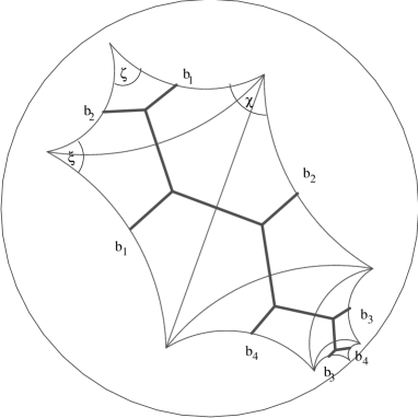
Figure 10: A “triangulated” geodesic polygon (thin geodesic arcs) representing the smooth surface $S$ on the unit disk. Edges are to be glued pairwise and with opposite orientation as indicated by the numbers and in accordance with relation (22) for the generators of the fundamental group. We have also included the original graph $\Gamma$ (thick lines).

3.3 The ZVC coordinates

In general the geodesic polygon is described by $6g$ parameters, namely, $4g$ angles and $2g$ side lengths. Since all of the angles contribute at the same base point $P$, they must sum up to $\sum_{i}\tilde{\alpha}_{i}=2\pi$. Assume now that $P$ is the intersection point of the smooth geodesics labeled $1$ and $2$, say, and that these two form part of the triangulation. In terms of the geodesic polygon this means that the two angles at $b_{1}$ ($\chi$ and $\zeta$ in Fig.10), as well as the two angles at $b_{2}$ ($\zeta$ and $\xi$) should add up to $\pi$. Together with the constraint $\sum_{i}\tilde{\alpha}_{i}=2\pi$ we therefore have three equations for the angles. The closure condition for the polygon makes two more sides and one angle redundant, and we arrive at $6g-6$ degrees of freedom. It is proven in [22] (see also [23]) that the so-called normal geodesic polygon corresponding to the above unique choice of base point characterizes the surface $S$ uniquely. In other words, going to the normal polygon amounts to a gauge fixing of the boost parameters $\eta_{i}$, which are the lengths of the arcs of the geodesic polygon, and can be calculated from the Zieschang-Vogt-Coldewey (ZVC) coordinates by using the triangle relations (12). In Appendix B we sketch the algorithm of how to construct a set of boost parameters corresponding to an element of ${\cal T}_{g}$ in practice.

3.4 The exchange transition

We have seen above how the boost parameters of a one-polygon tessellation can be used to characterize a surface $S$ uniquely. However, as we have pointed out already, within a finite amount of time $\Sigma$ may undergo a transition which changes both $\Gamma$ and its dual $\gamma$. In the absence of particles and concave angles only one transition can take place, the so-called exchange transition. As illustrated by Fig.11, the shrinking away of edge 5 of $\Gamma$ (with boost parameter $\eta_{5}$) and subsequent “birth” of edge 5’ (with boost parameter $\eta_{5}^{\prime}$) amounts to a “flip move” on the associated triangulation, namely, the substitution of one diagonal of a quadrilateral by its dual diagonal, whose length can be obtained by elementary trigonometry. At the level of $S$, this operation corresponds to an elementary move on the associated triangulation of $S$ as discussed in subsection 3.2 above. The surface $S$ itself remains unchanged, and is therefore invariant under the time evolution. (Note that this does not imply the absence of time evolution from the original picture, but only reflects the constancy of the edge momenta or velocities.) That $S$ is also left invariant by the residual Lorentz gauge transformations of the polygon model will be demonstrated in the next subsection.

Figure 11: During an exchange move, the boost parameter $\eta_{5}$ changes to $\eta_{5}^{\prime}$. All new angles are determined unambiguously. Edges of $\Gamma$ are drawn as solid, arcs of the dual triangulation $\gamma$ as dotted lines.

3.5 Lorentz transformation

An important issue we have not addressed so far is the role played by the choice of base point in $S$. As we will show in the following, the action of a Lorentz transformation on the boost parameters (that is, a symmetry transformation of the piecewise flat formulation) precisely induces a change in the location of the base point. Recall the matching condition

$$\Lambda_{1}X_{1}+a_{1}=X_{2}$$ (26)

between neighbouring coordinate systems $X_{1}$ and $X_{2}$ in the polygon picture. If the edge in question separates two distinct polygons, the corresponding coordinate systems $X_{1}$ and $X_{2}$ can be Lorentz-transformed with independent group elements. In the special case of a one-polygon tessellation we have only one coordinate system, and $X_{2}$ is just an (auxiliary) copy of $X_{1}$. Under the action of a Lorentz transformation $\Lambda$ we have $X_{j}\to\tilde{X}_{j}=\Lambda X_{j}$, $j=1,2$, and the matching condition gets modified to

$$\tilde{\Lambda}_{1}\tilde{X}_{1}+\tilde{a}_{1}=\tilde{X}_{2}$$ (27)

with $\tilde{\Lambda}_{1}=\Lambda\Lambda_{1}\Lambda^{-1}$ and $\tilde{a}_{1}=\Lambda a_{1}$.

To see the effect of this transformation on the triangulation of $S$, it is convenient to use a different representation of $S$. Any Riemann surface $S$ with genus $g>1$ can be represented as a quotient $H/G^{\prime}$, where $H$ is the hyperboloid $\{(t,x,y)|-t^{2}+x^{2}+y^{2}=-1\}$ with $ds^{2}$ inherited from the three-dimensional Minkowski space and the subgroup $G^{\prime}\subset SO(2,1)$ is isomorphic to the fundamental group $\pi_{1}(S)$. For simplicity we will use the isomorphic quotient $D^{2}/G$ instead, where $D^{2}$ is the open unit disk with line element

$$ds^{2}=\frac{4|dz|^{2}}{(1-|z|^{2})^{2}}$$ (28)

and $G\subset$ PSU$(1,1)$ (PSU$(1,1)$ is isomorphic to $SO(2,1)$). The group action on points $z$ of the unit disk is given by

$$z\mapsto gz=\frac{g_{11}z+g_{12}}{g_{21}z+g_{22}}.$$ (29)

We use PSU$(1,1)=SU(1,1)/\mathbb{Z}_{2}$, because any element $g\in SU(1,1)$ has the same action on the coordinate $z$ as $-g$. Identifying boost and rotation matrices,

$$b(\xi):=\left(\begin{array}[]{cc}\cosh\frac{\xi}{2}&\sinh\frac{\xi}{2}\\ \sinh\frac{\xi}{2}&\cosh\frac{\xi}{2}\end{array}\right),\quad r(\phi)\>=\left(\begin{array}[]{cc}\exp(i\frac{\phi}{2})&0\\ 0&\exp(-i\frac{\phi}{2})\end{array}\right),$$ (30)

any PSU(1,1) matrix can be written as

$$g=r(\phi)b(\xi)r(\phi^{\prime}),$$ (31)

and the isomorphism with SO(2,1) is given by $B(\xi)\leftrightarrow b(\xi)$ and $R(\phi)\leftrightarrow r(\phi)$, cf. (7). Consider now a universal cover $f:D^{2}\to S$ of the surface $S$, and let $z_{0}$ be an inverse image of the base point $P\in S$. Consider the $2g$ lifts of the geodesic loops corresponding to the $2g$ standard generators $b_{i}$ of $\pi_{1}(S)$. There is a unique element $g_{i}$ in $G$ which maps $z_{0}$ to the other end point of the lift of $b_{i}$, which is a geodesic arc in $D^{2}$. When decomposing the group element $g_{i}$ according to eq.(31), the boost parameters are identified with the parameters $\xi_{i}$ (the lengths of the arcs connecting $z_{0}$ and $g_{i}z_{0}$) according to $2\eta_{i}=\xi_{i}$. The elements of the Teichmüller space ${\cal T}_{g}$ are in one-to-one correspondence with the conjugacy classes of discrete subgroups of $PSU(1,1)$, that is, $G$ and $hGh^{-1}$ with $h\in$PSU(1,1) determine the same surface $S$. If the base point for the action of $G$ was $f(z_{0})\in S$, it is $f(hz_{0})$ for $hGh^{-1}$, where the generators of $hGh^{-1}$ are simply obtained by conjugating the standard generators with $h$. Like the action of the corresponding $\Lambda\in SO(2,1)$ by conjugation (defined below (27)), the action of $h\in$PSU(1,1) has a non-trivial (one-dimensional) isotropy group. This completes the argument that a Lorentz transformation on the coordinate system associated with the polygon translates into a change of the base point of the triangulation of $S$, while leaving the surface $S$ itself unchanged.

3.6 The complex constraint

While we have found an abstract geometric re-interpretation for the boost parameters of the polygon representation, which has enabled us to identify the independent physical and the redundant gauge degrees of freedom, nothing has been said so far about the other half of the canonical variables, the edge length variables $\{L_{i}\}$. We will show in the following that the complex constraint (19) admits a solution for any triangulation of any surface $S\in{\cal T}_{g}$, provided that the base point $P\in S$ is chosen carefully. Furthermore, we will show that from a particular solution (of eq.(36) for all relevant triplets $z_{i}$) one can construct a $(6g-6)$-parameter family of solutions, thus spanning an entire sector $\cal P$ of the full phase space where ${\cal P}=\mathbb{R}_{+}^{6g-6}\times{\cal T}_{g}\stackrel{{\scriptstyle\rm diff}}{{=}}\mathbb{R}^{12g-12}$.

For the case at hand, we can rewrite the complex constraint (19) as

$$\sum_{I=1}^{6g-3}L_{I}z_{I}=0$$ (32)

with $z_{I}=\exp(i\theta_{i})+\exp(i\theta_{j})$, since each label I will appear exactly twice, namely, at positions $i$ and $j$ when counting the edges of the polygon in counterclockwise direction. The angles $\theta_{i}$ are expressible as sums of angles $\alpha_{i}$ of the polygon, but there is a more straightforward way of writing them.

Figure 12: Starting from the edge labeled $1$ and proceeding in counterclockwise direction one has $I(1)=1,\>I(2)=2,\>I(3)=3,\>I(4)=1$, $\dots$ and therefore $z_{1}=\exp(i\theta_{1})+\exp(i\theta_{4})$. Instead of adding the outer angles in terms of $\alpha_{i}$ to obtain $\theta_{i}$, we can determine them directly from the angle parameters appearing in the Lorentz transformation part of the matching conditions corresponding to the edge $1$.

If the matching condition was $X_{2}=\Lambda_{1}X_{1}+a_{1}$ with

$$\Lambda_{1}=R(\phi_{1})B(2\eta_{1})R(\phi^{\prime}_{1}),$$ (33)

one can rewrite it as $R(-\phi_{1})X_{2}=B(2\eta_{1})R(\phi_{1}^{\prime})X_{1}+a^{\prime}_{1}$, and Fig.12 then shows that

$$\theta_{1}=\phi_{1},\quad\theta_{4}=\pi-\phi^{\prime}_{1}.$$ (34)

In order to derive this relation, one has to take into account that (after an appropriate translation) $X_{2}$ has to be rotated by an angle $-\phi_{1}$ and $X_{1}$ by an angle $\phi^{\prime}_{1}$ to align their spatial axes with those of $X$, and that the two occurrences of an edge always have opposite orientation. After rotating the spatial axes of $X_{1}$ and $X_{2}$ to those of $X$, the matching condition between the new coordinate systems is a pure boost $B(2\eta_{1})$. The coefficient $z_{1}$ of the corresponding edge is therefore given by

$$z_{1}=\exp(i\phi_{1})+\exp(i(\pi-\phi^{\prime}_{1})).$$ (35)

The constraint (32) is a complex linear equation, and has a solution if and only if the complex coefficients $z_{i}$ – thought of as vectors based at the origin of the complex plane – are not contained in a half plane. If they are, there is no non-trivial linear combination with positive coefficients $L_{i}$ which vanishes. In Appendix C we prove the non-trivial fact that after an appropriate conjugation of the generators $g_{i}$ of $G$ which correspond to the loops of the triangulation, the coefficients $z_{i}$ will be transformed into a generic position, not contained in any half plane.

Suppose now that this has been achieved, ie. there are three points $z_{1}$, $z_{2}$, $z_{3}$ in the desired generic position. We can divide the complex plane as depicted in Fig.13, and $z_{i}$, $i>3$, is some other point lying in the convex section of the plane bounded by lines $1$ and $3$, say. Then the equation

$$\lambda_{1}z_{1}+\lambda_{2}z_{3}+(1-\lambda_{1}-\lambda_{2})z_{i}=0$$ (36)

admits a unique solution with $\lambda_{1},\lambda_{2},\lambda_{1}+\lambda_{2}\in]0,1[$.

Figure 13: For any point $z_{i}$ ($i>3$) in one of the convex sections of the complex plane bounded by two half lines $j,k\in\{1,2,3\}$, the triangle with corner points $(z_{i},z_{j},z_{k})$ contains the origin. In other words, the corresponding eq.(36) has a unique solution with $\lambda_{j},\lambda_{k},\lambda_{j}+\lambda_{k}\in]0,1[$.

A similar statement holds for any point $z_{i}$ contained in one of the other two convex sections of the plane. There are $6g-5$ independent triangles ($(1,2,3)$, and every other index $i\in[4,6g-3]$ matched with two of $(1,2,3)$ according to the location of $z_{i}$ as explained above). Adding up the resulting $6g-5$ equations of the form (36), each one multiplied by an arbitrary number $\rho_{i}>0$, we get a solution to the constraint (32). Each index is represented, and each $z_{i}$ appears with a positive coefficient $L_{i}$, namely, a positive linear combination of the $\rho_{j}$. All $\rho_{i}$’s are independent, but we can fix $\rho_{1}$ to be $1$, which fixes the global time parameter or, equivalently, an overall length scale. Thus we have completed the explicit construction of a $(12g-12)$-parameter set $\cal P$ of independent and unconstrained initial conditions for the polygon model, each corresponding to a one-polygon universe. We have obtained this space in the explicit form ${\cal P}={\mathbb{R}}_{+}^{6g-6}\times{\cal T}_{g}$. We conjecture in Sec.4 below that $\cal P$ is identical with the full phase space of the model, and not just an open subset of it.

4 Multi-polygon tessellation and smooth surface

What we have described up to now is the sector of the theory corresponding to a single polygon. For this case, we have identified a complete set of initial data (the phase space $\cal P$), and shown that it is mapped into itself under time evolution. However, as we have mentioned in the introduction, a generic universe in the ’t Hooft representation is a whole collection of flat polygons glued together at their boundaries. We will in the following prove a number of results about multi-polygon configurations, and discuss their relation to the one-polygon sector of the theory. Because of technical problems to do with the complicated action of the Lorentz gauge transformations on these configurations, we have so far been unable to establish explicit solutions to the analogues of the constraint equation (32) and to construct a complete set of initial data. These questions may ultimately turn out to be irrelevant if a conjecture of ours is correct, namely, that any multi-polygon universe is physically equivalent to one in the one-polygon sector described in the previous section.

A universe consisting of $F$ polygons has a graph $\Gamma$ with $6g+3(F-2)$ edges. Since every edge comes with a canonical variable pair $(\eta_{i},L_{i})$, it is clear that $3F$ of these pairs must correspond to unphysical or redundant information. For $F>1$, one would expect that at the level of the $\eta$’s alone three more boosts can be gauge-fixed for every additional polygon in the tessellation. We will illustrate below by a specific example how a multi-polygon universe can be effectively reduced to a universe with fewer polygons by a suitable gauge-fixing.

We will begin by explaining how our method of associating a unique set of Teichmüller parameters to every universe generalizes to the case of more than one polygon. At the level of the piecewise flat physical Cauchy surface $\Sigma$, the dynamics of a multi-polygon tessellation involves also other types of transitions [11] which in general will change $F$, and which we will describe next. As a new feature of the multi-polygon case, we will see that the boost parameters can now have different signs. Finally, we will discuss gauge-fixing and formulate our conjecture.

4.1 Multi-polygon tessellation

We have already explained in the introductory part of Sec.3 how to associate a unique smooth uniformized surface with a geodesic triangulation $\tilde{\gamma}$ to every pair $(\Sigma,\Gamma)$. Like the dual graph $\gamma$, $\tilde{\gamma}$ still has $F$ base points and $6g+3(F-2)$ geodesic “edges”. Since the set of $\eta$’s carries a redundancy, one cannot read off directly the Teichmüller parameters which characterize the hyperbolic surface $S$ uniquely. However, there is a straightforward procedure to effectively reduce the graph $\tilde{\gamma}$ to that of a normal geodesic polygon (cf. Sec.3.3 above), with a minimal number $6g-3$ of edges. It involves the “gauging away” of a number of geodesic arcs which link different base points $\tilde{P}_{i}$, so they can all be thought of as one and the same base point corresponding to a one-polygon configuration. Details of the procedure can be found in Appendix D.

4.2 Transitions for multi-polygons

For the case $F>1$, four more transitions can occur during the course of the time evolution, in addition to the “exchange move” already discussed in Sec.3.4. The new transitions are qualitatively different since individual edges of $\Gamma$ may collapse to zero length, or new edges may be generated when a vertex at a concave angle hits the opposite side of a polygon. Those of the transitions which change the number $F$ of polygons (and therefore of edges) are awkward to deal with, since they correspond to “jumps” in the number of dynamical variables before taking constraints and gauge symmetries into account. The evolution of the physical phase space variables is of course perfectly well-defined and unique during these transitions as was shown in [11, 17], but this is not the form in which the theory is given in the first place.

Let us enumerate the new transitions one by one and study what effect they have on the dual triangulation $\tilde{\gamma}$. The transitions will also play a role when considering finite gauge transformations, cf. subsection 4.3 below.

1. vertex grazing: $F\to F,\;\eta\to-\eta$

   As is clear from Fig.14, this transition does not change the triangulation $\gamma$, in agreement with the fact that the order of boundary edges around each polygon remains the same. The absolute value of the boost parameter of the shrunk edge does not change, but its sign does.

2. triangle disappearance: $F\to F-1$

   The time reversal of this transition gives a refinement of the triangulation $\gamma$. Fig.15 shows that the corresponding base point $S$ disappears. The three dual edges emanating from $S$ are therefore “deleted”, as well as the corresponding edges of the polygon(s).

3. double triangle disappearance: $F\to F-2$

   Like in the previous transition, the time reversal of this one is also a refinement, as illustrated in Fig.16. Note that the two curves connecting $P$ and $Q$ lie in the same homotopy class in $S$ so their corresponding (absolute values of) boost parameters must coincide even though they correspond to different edges of $\Gamma$.

4. vertex hit: $F\to F+1$

   This transition corresponds directly to a refinement of the triangulation $\tilde{\gamma}$. Fig.17 shows a somewhat misleading picture, since the points $P$ and $P^{\prime}$ are actually the same, but correspond to different polygons. In other words, $PS$ and $P^{\prime}S$ are different curves in $\gamma$ but coincide in $\tilde{\gamma}$ on $S$. The three new edges are the arcs $QS$, $RS$ and $P^{\prime}S$, a duplicate of $PS$.

Figure 14: Vertex grazing.

Figure 15: Triangle disappearance.

Figure 16: Double triangle disappearance.

Figure 17: Vertex hit.

4.3 Reducing multi-polygons by gauge-fixing

In order to illustrate the relation between tessellations with different numbers $F$ of polygons, let us consider an explicit example. Fig.18 represents a tessellation with $F=2$, corresponding to the piecewise flat universe of Fig.7. The figure is analogous to Fig.10 (before mapping it to $S$) with the difference that the dual graph $\gamma$ (dotted lines) now has two distinct base points $P$ and $Q$ as indicated. The solid lines represent edges of $\Gamma$. Any such edge which reaches the boundary of the big quadrilateral must be glued to the outgoing edge labeled by the same number. The two flat polygons corresponding to this example are shown schematically in Fig.19. Closed dual loops based at $P$ ($Q$) correspond to edges which appear twice in the polygon with centre $P$ ($Q$), and dual curves connecting $P$ to $Q$ correspond to edges appearing in both polygons. After the gluing the two polygons form a connected piecewise flat surface of genus 2.

Figure 18: Alternative schematic representation of the $F=2$ universe corresponding to Fig.7, showing both the graph $\Gamma$ (solid lines) and its dual $\gamma$ (dotted lines). The boundary edges of the rectangle (corresponding to smooth geodesic arcs) must be glued pairwise with opposite orientation, such that the open edges of $\Gamma$ are glued pairwise according to matching numbers. In the corresponding graph $\tilde{\gamma}$ on $S$, moving $P$ to $Q$ along the dual edge $3$ results in the degeneration of triangles $348$ and $239$. Simultaneously, the two polygon angles indicated on the figure as well as the sums of the other two angles at both vertices become $\pi$, edge 3 becomes redundant, the two vertices do not carry deficit angle any more and 48 and 29 can be thought of as the same edge. The configuration becomes effectively that of a one-polygon universe.

Consider now the situation when one of the dual edges, say, edge 3, has zero length. The base points $P$ and $Q$ then fall on top of each other, and the triangles $348$ and $392$ are degenerate, since the two edges $4$ and $8$ coincide, as do $2$ and $9$. The angles enclosed by these pairs of edges are zero, and consequently the angles between the edges of $\Gamma$ (indicated in Fig.18) on the piecewise flat surface are $\pi$. Furthermore, since the boost parameter is zero, the matching condition in the most general case is given by

$$X_{P}=R(\phi)X_{Q}-a.$$ (37)

This implies we can redefine $X_{Q}$ to be exactly $X_{P}$ without changing the shape of the polygon (since the transformation is a pure rotation). It also means that edge $3$ is redundant, and edges $4$ and $8$ (as well as $2$ and $9$) can be represented by just single edges. We have therefore rederived the situation of Fig.8.

Figure 19: The polygons corresponding to the two-polygon universe of Figs.7 and 18. If one Lorentz-transforms the two coordinate frames such that $\eta_{3}$ becomes zero, the angles $\theta+\omega$ and $\epsilon$ between edges $2$ and $9$ become $\pi$. Similar statement holds for edges $4$ and $8$. Switching to the one-polygon representation of the same universe amounts to deleting edge $3$ and the vertices on it (which no longer carry any deficit angles) and considering $2$ and $9$ as well as $4$ and $8$ as single edges.

The intriguing conclusion from this analysis is that the boost parameter of an edge bounding two distinct polygons can always be made to vanish by an appropriate gauge transformation. The general matching condition of edge $3$ (omitting the translational part) reads

$$X_{P}=\Lambda X_{Q},$$ (38)

where $X_{P}$ and $X_{Q}$ are now distinct coordinate systems. After performing two independent Lorentz transformations on both frames ($X_{P}\to\tilde{X}_{P}=\Lambda_{P}X_{P}$ and $X_{Q}\to\tilde{X}_{Q}=\Lambda_{Q}X_{Q}$) eq.(38) becomes

$$X_{P}=\Lambda_{P}^{-1}\Lambda\Lambda_{Q}X_{Q}.$$ (39)

There are now many choices for $\Lambda_{P}$ and $\Lambda_{Q}$ which reduce the matching condition to $X_{P}=X_{Q}$ (for example, $\Lambda_{P}=\Lambda$ and $\Lambda_{Q}=I$ will do), which means that we can effectively get back to a one-polygon tessellation by performing a symmetry transformation. By iterating this argument, one can reduce any multi-polygon to one equivalent to a single polygon (cf. Appendix D), while leaving the smooth surface $S$ unchanged.

However, there is a caveat which prevents us from proving the physical equivalence of any multi-polygon universe with a one-polygon universe. Note that in performing the finite Lorentz transformations of local Minkowski frames to gauge-fix some of the $\eta$’s, we have so far completely ignored how these transformations act on the shapes of the polygons. Although infinitesimal Lorentz transformations of this type can always be performed, for larger transformation one will in general encounter the same transitions that can occur during time evolution, and therefore be forced to switch to a new set of edge variables. For example, due to a concave vertex hitting an opposite edge, any one-polygon component may decompose into several pieces, thus defeating the aim of reducing the number of polygons.

In other words, we may not be able to “lift” the action of any given Lorentz transformation on the angle variables $(\eta_{i})$ to one on the full set $(L_{i},\eta_{i})$ of phase space variables for a given set $e_{i}$ of edges. This potential obstruction to reduction is not as bad as it may at first appear, since already at the level of the $\eta$’s the reduction is highly non-unique. Unfortunately, the action of the symmetry group on the phase space is rather involved and to find elements in $\times_{F}$PSU(1,1) which avoid transitions which increase $F$ seems to depend on the details of the geometry of the multi-polygon universe. We have so far neither a general argument nor an explicit algorithm for reducing any given universe to one equivalent to a one-polygon universe, but only a

Conjecture. For any multi-polygon universe given in terms of $6g+3(F-2)$ pairs of edge variables $(L_{i},\eta_{i})$, one can always find a joint frame transformation in
$\times_{j=1}^{F}$PSU(1,1)_j which avoids transitions and leads to a gauge-equivalent configuration with only $6g-3$ non-vanishing variable pairs, and physically equivalent to a one-polygon universe.

If the conjecture is true, the solution space $\cal P$ associated with one-polygon universes we constructed in Sec.3 coincides with the full physical reduced phase space of pure (2+1) gravity for compact slices of genus $g$.

5 Discussion

By re-interpreting the boost parameters of ’t Hooft’s polygon model as geodesic lengths on a hyperbolic surface $S$ of constant curvature $R=-1$ we have succeeded in finding an explicit parametrization of a sector $\cal P$ of dimension $12g-12$ of the physical phase space of the model. The lengths are those of the geodesic loops and arcs of a triangulation of $S$, whose vertices are in one-to-one correspondence with the polygons of the physical Cauchy surface. At the level of $S$, the action of the gauge transformations of the polygon model is well understood, and corresponds to moving the vertices of the triangulation.

If there is only a single vertex, the corresponding constant-time slice of the (2+1) universe consists of one polygon. For this case, we have solved the complex initial-value constraint of the model, and have given a complete parametrization of the solution space $\cal P$ of initial data. This was done by expressing the boost parameters as functions of the Teichmüller parameters of $S$, and then complementing them by suitable edge length variables which solve the initial value constraint. We conjecture that $\cal P$ coincides with the full phase space of (2+1) vacuum gravity. Equivalently, we conjecture that any multi-polygon tessellation is physically equivalent to a one-polygon tessellation. We also showed that time evolution in $\cal P$ is either eternal expansion from a big bang or shrinking to a big crunch from the infinite past, thus generalizing a known result from the genus-1 case.

A natural next step in our analysis will be the inclusion of point particles. In the case without particles treated in this paper, the generators $g_{i}$ are hyperbolic elements of PSU(1,1) ($|$tr$\>g_{i}|>2$), which have no fixed points in $D^{2}$. The generator corresponding to a particle on the other hand will be elliptic ($|$tr$\>g_{i}|<2$). It has a fixed point in $D^{2}$ (since it is conjugate to a rotation), and the corresponding hyperbolic structure $D^{2}/G$ will have singular points as expected. We believe that the method introduced in this paper can be generalized to this case, by substituting the smooth surface $S$ by one with a number of punctures, one for each particle.

Another issue one might like to investigate is the role played by the mapping class group G in the higher-genus case. Its action is not difficult to describe: a Dehn twist is obtained by conjugating the generators $g_{i}$ of $G$ by a group element $h\in G$. What kind of further redundancies this may induce on the phase space and whether those can at all be “factored out” are in general very difficult issues. (For contradictory claims in the torus case, see [25, 26].

This work – motivated by having a computer code but being unable to produce a set of initial data solving the constraints – is a step toward understanding the asymptotic behaviour of 2+1 gravity near the singularity and other dynamical issues about which very little is currently known for higher-genus universes. A numerical treatment is now feasible, but also analytical progress may be within reach. A beautiful feature of the ’t Hooft model is the simplicity of its dynamics, since all the length variables $L$ evolve linearly. As we have seen, this picture is partially spoiled by the presence of “transitions”, points in the evolution at which the number of phase space variables (before imposing the constraints) jumps. If our conjecture is indeed true, it would mean that such transitions can be completely avoided, leading to a considerable simplification of both the classical and potentially also the quantum theory.

Appendix A Boosts in the one-polygon tessellation

In this appendix we prove that a one-polygon tessellation only admits configurations where all boost parameters have the same sign. Recall that $\pi<\sum_{i}\alpha_{i}<2\pi$ holds for mixed vertices $v$ of $\Gamma$, and $2\pi<\sum_{i}\alpha_{i}<3\pi$ for the homogeneous ones. Since the graph $\Gamma$ has $4g-2$ vertices, in the case of two mixed vertices the sum of all angles in the polygon is given by (cf. (18))

$$(12g-8)\pi=\sum_{i=1}^{12g-6}\alpha_{i}<4\pi+(4g-4)3\pi=(12g-8)\pi.$$ (40)

This is a contradiction, so we can exclude the appearance of more than one mixed vertex. Note that if the graph $\Gamma$ was one-particle irreducible we would already be done, since there cannot be only a single mixed vertex in such a graph.

Suppose then that one vertex $v_{0}$ is mixed. For the sum of the angles of all hyperbolic triangles we have

$$\sum_{i=1}^{12g-6}\tilde{\alpha}_{i}=2\pi,$$ (41)

since all of them contribute at the base point of the triangulation $\gamma$, and this point does not carry a non-trivial deficit angle. Next, recalling that at the mixed vertex $\alpha_{3}=\tilde{\alpha}_{3}+\pi$ and $\alpha_{1}=\tilde{\alpha}_{1},\;\alpha_{2}=\tilde{\alpha}_{2}$, the polygon closure constraint is given by

$$\begin{array}[]{l}{\displaystyle\sum_{i=1}^{12g-6}\alpha_{i}=\sum_{i\;{\rm not\,at}\,v_{0}}(\pi-\tilde{\alpha}_{i})+\tilde{\alpha}_{1}+\tilde{\alpha}_{2}+\tilde{\alpha_{3}}+\pi=}\\ {\displaystyle=(4g-3)3\pi+\pi+\sum_{i\;{\rm at}\,v_{0}}\tilde{\alpha_{i}}-\sum_{i\;{\rm not\,at}\,v_{0}}\tilde{\alpha_{i}}=(12g-8)\pi}.\end{array}$$ (42)

The last equality is the requirement of the constraint. Relation (42) implies that

$$\sum_{i\;{\rm at}\,v_{0}}\tilde{\alpha}_{i}-\sum_{i\;{\rm not\,at}\,v_{0}}\tilde{\alpha}_{i}=0,$$ (43)

which in conjunction with eq.(41) leads to

$$\sum_{i\;{\rm at}\,v_{0}}\tilde{\alpha_{i}}=\pi$$ (44)

for the triplet of angles associated with $v_{0}$. This means that the corresponding hyperbolic triangle is degenerate since its area vanishes, $\pi-\sum_{i}\tilde{\alpha_{i}}=0$. As a consequence, either two of its sides coincide and the third one has length zero, or the union of its two short sides with angle $\pi$ between them coincides with the long side. The first case is again excluded since $\eta_{i}=0$ implies two vertices having no deficit angle which again leads to an inconsistency in (40). (Although the contribution of the mixed vertices on the right-hand side is maximized to $4\pi$, the homogeneous vertices still contribute with angle sums strictly smaller than $3\pi$.) The second case corresponds to the situation where $\alpha_{i}=0$ for some $i$, which is not allowed.

Appendix B Boost parameters from Teichmüller space

In this appendix we will explain how to obtain an independent set of initial values for the boost parameters $\eta$. For simplicity and illustrative purposes, we will discuss an example of genus 2. Since we will not make use of the symmetry structure of this particular case, the generalization to higher genus is immediate.

We fix the triangulation by choosing the graph $\Gamma$ on Fig.8, leading to the triangulation of Fig.9. We will use the convention of multiplying loops from left to right. The numbers indicate the outgoing ends of the loops, and $i=1,\dots,4$ label the generators $b_{i}$ of the fundamental group satisfying $b_{1}b_{2}b_{1}^{-1}b_{2}^{-1}b_{3}b_{4}b_{3}^{-1}b_{4}^{-1}=1$. The homotopy classes of the remaining closed curves can be obtained by composing the fundamental generators and their inverses, leading to

$$\begin{array}[]{ccl}5&\to&b_{2}b_{1}b_{2}^{-1}b_{1}^{-1}\\ 6&\to&b_{1}b_{2}^{-1}\\ 7&\to&b_{2}b_{1}b_{2}^{-1}\\ 8&\to&b_{3}b_{4}^{-1}\\ 9&\to&b_{4}b_{3}b_{4}^{-1}.\end{array}$$ (45)

Now we use the faithful representation of $\pi_{1}(S)$ in PSU$(1,1)$ given explicitly in [24] in terms of the so-called Fenchel-Nielsen coordinates. They are a set of length and angle variables $(l_{k},\tau_{k})$, $k=1,\dots,3g-3$, which parametrize the Teichmüller space ${\cal T}_{g}$ globally. One can pick an arbitrary element $(l,\tau)\in{\mathbb{R}}_{+}^{3g-3}\times{\mathbb{R}}^{3g-3}\cong{\cal T}_{g}$, plug it into the formulae for the generators $g_{i}\in$ PSU(1,1) and compute the combinations for the group elements corresponding to the remaining curves in the triangulation (in our specific example, the curves labeled 5, 6, 7, 8 and 9). Now, knowing the group generators and the combinatorial information (the order of the edges going around the polygon), we can identify the boost parameters and compute the angles as well. How the boosts are supplemented by a set of length variables $L_{i}$ has been described in Sec.3.6 above. Altogether this amounts to an explicit algorithm for constructing a set of initial data for a (2+1)-dimensional universe from any element of ${\mathbb{R}}_{+}^{6g-6}\times{\cal T}_{g}$.

Appendix C The complex constraint

The proof that for a one-polygon tessellation there is always a Lorentz frame in which the complex constraint (32) admits a solution rests on the following facts.

1. The complex vector $z_{i}$ defined below eq.(32) points to the angle bisector of the geodesic loop corresponding to $g_{i}$.

2. The velocity at $P$ of the unique arc connecting the base point $P\in S$ to the unique smooth closed geodesic corresponding to $g_{i}$ points in the same direction.

3. One can find a base point where these velocities are not contained in a half plane.

4. In practice one proceeds by finding an element $h\in$PSU(1,1) which corresponds to the desired change of base point. The original vectors $z_{i}$ can be read off from $g_{i}\in G$. The new coefficients $z_{i}^{\prime}$ will be determined from the conjugated generators $h^{-1}g_{i}h$, and they will not lie in a half plane by the above arguments.

Take the universal cover where the origin $0\in D^{2}$ is mapped to the base point $P\in S$. The in- and out-going ends of the loop $g_{i}$ on $S$ can be associated with the geodesic arcs connecting $0$ with $g_{i}0$ and $0$ with $g^{-1}_{i}0$ (the group action on points $z\in D^{2}$ was defined in eq.(29)). Since the geodesics through $0\in D^{2}$ are Euclidean straight lines, and since

$$g_{i}0=\tanh\eta_{i}\exp i\phi_{i},\quad g_{i}^{-1}0=\tanh\eta_{i}\exp i(\pi-\phi^{\prime}_{i}),$$ (46)

it is clear that the angle bisector of $g_{i}0$ and $g^{-1}_{i}0$ points in the same direction as $z_{i}$.

The next step is to establish the validity of Fig.20, namely, that the two quadrilaterals $Pqrs$ are isometric. The figure shows the smooth geodesic (inner circle) freely homotopic to the geodesic loop $PP$ and the unique smooth geodesic arcs $Pq$ and $rs$ connecting two, and perpendicular to them in the points $q$, $r$ and $s$. All we need to show is that the arc $Pq$ is the angle bisector of the velocities of the in- and outgoing ends of the loop (denoted by $\eta$ in the figure). We refer to [23] for a detailed proof. The properties of the various geodesics in $D^{2}$ are illustrated by Fig.21. The smooth geodesic of Fig.20 is mapped to the smooth straight line on the bottom, and the geodesic loop to the periodic non-smooth curve at the top. The curves at $q$, $r$ and $s$ meet at right angles.

Figure 20: On the surface $S$, the loop connecting the basepoint $P$ to itself via point $s$ is the loop in the triangulation corresponding to $g_{i}$. The circle in the middle is the unique smooth geodesic which lies in the same homotopy class as the loop. The unique arcs connecting $P$ to the circle and the circle to the loop such that the angles at $q$, $r$ and $s$ are right angles create two isometric quadrilaterals.

Figure 21: Lift to $D^{2}$ of a (periodically extended) geodesic loop at $P$ (top) and of the associated homotopic smooth geodesic (bottom). The geodesic arc $rs$ is the unique perpendicular connecting the geodesic loop $PP$ to the smooth closed geodesic $qq$. The unique geodesic arc connecting $P$ to $qq$ which is perpendicular at $q$ is the angle bisector of the loop and its inverse at $P$. The thick lines indicate one of the (infinitely many) pairs of isometric quadrilaterals $Pqrs$ (each with three right angles) which are mapped to Fig.20 under the universal covering map $f$.

The situation on $D^{2}$ is as follows. We are given the set of $6g-3$ elements $\{g_{i}\}$ of the fundamental group $G$. Each $g_{i}$ has its so-called axis, that is, the geodesic which is left invariant by $g_{i}$. On the disk $D^{2}$, an axis has the form of a circle segment whose ends are perpendicular to the disk boundary. (This fact is not reproduced in Fig.21, where the axis is represented by the straight line at the bottom.) Under the universal cover, an axis is mapped (infinitely many times) to the smooth geodesic on $S$ corresponding to $g_{i}$. The unique geodesic arc on $D^{2}$ from the origin which is perpendicular to one of these axes is mapped to the arc on $S$ connecting the base point to the smooth geodesic in question.

Suppose now that their initial velocities at the origin are contained in a half plane (otherwise we are already done). We can then find a point $T\in D^{2}$, such that the initial velocities of the unique arcs – emanating from $T$ and perpendicular to the axes – do not lie in a half plane. The procedure for finding such a location is straightforward, and is illustrated in Fig.22. Pick two loops $g_{1}$ and $g_{2}$ based at $P$ whose associated smooth geodesic loops do not intersect. Consider the mid point $M$ of the unique geodesic arc perpendicular to both of the associated axes, $l_{1}$ and $l_{2}$. If we were to choose $M$ as the new base point, the two oppositely oriented tangent vectors to the arc at $M$ would define the directions of the new complex vectors $z_{1}^{\prime}$ and $z_{2}^{\prime}$. There are then two possibilities. (i) The remaining axes $l_{i}$, $i\geq 3$, do not lie just to one side of the arc, so that their tangent vectors at $M$ already span the entire two-plane. In this case we are done and $T\equiv M$ is a good new base point. (ii) The remaining axes lie to one side of the arc only, so that their tangent vectors, together with $z_{1}^{\prime}$ and $z_{2}^{\prime}$ span only a half plane. For example, in Fig.22 they all lie like $l_{3}$, that is, below the arc. In that case it will be sufficient to move the point to a new point $T$ slightly away from the arc, in the direction of the remaining axes. The new tangent vectors $z_{1}^{\prime\prime}$ and $z_{2}^{\prime\prime}$ will then enclose an angle slightly smaller than $\pi$, and together with $z_{3}^{\prime\prime}$, say, span the entire two-plane.

Figure 22: The circle segment $l_{i}$ perpendicular to the disk boundary is the so-called axis of $g_{i}$. In the figure, $g_{1}$ and $g_{2}$ correspond to two non-intersecting smooth geodesics. A good new base point $T$ is either given by the mid point of the unique arc orthogonal to both $l_{1}$ and $l_{2}$ (dashed line), or by moving slightly away from the mid point and from the arc, as explained in the text. In the figure, after moving $T$ to a location below the arc (as indicated in the magnified picture of the neighbourhood of the mid point on the right), the three initial velocities of the unique geodesics connecting $T$ with $l_{1}$, $l_{2}$ and $l_{3}$ (and perpendicular to them) will span the entire two-plane.

In either case, a suitable new base point on $S$ is the image of $T$ under the universal cover. For calculational purposes, it is convenient to change the universal cover to another one whose origin is mapped to the new base point. The effect of this is to conjugate $g_{i}\to h^{-1}g_{i}h$. The triangulation in $D^{2}$ determined by the set $\{g_{i}\}$ with base point $T$ is isometric to that determined by $\{h^{-1}g_{i}h\}$ with base point $0$, with

$$T\to h^{-1}T=0,\quad g_{i}T\to h^{-1}g_{i}h0=h^{-1}g_{i}T.$$ (47)

We have thus completed the proof that one can always find a Lorentz frame in which the complex constraint admits a solution.

Appendix D Eliminating polygons by gauge-fixing

In this appendix we will show how to gauge-transform a given $(\tilde{\gamma},F)$ (a geodesic triangulation $\tilde{\gamma}$ of some $F$-polygon) to a configuration $(\tilde{\gamma}^{\prime},F)$ which is equivalent to a configuration $(\tilde{\gamma}^{\prime\prime},F-1)$ with one polygon fewer. The induced map $(\tilde{\gamma}^{\prime},F)\mapsto(\tilde{\gamma}^{\prime\prime},F-1)$ amounts to deleting three edges and one base point from $\tilde{\gamma}^{\prime}$ but does not change $\tilde{\gamma}^{\prime}$ as a point set.

A gauge transformation of $(\tilde{\gamma},F)$ is an action of $\times_{F}$PSU(1,1), where each of the $F$ copies of PSU(1,1)$\equiv$ SO(2,1) acts independently as follows. If $\tilde{e}_{ij}$ denotes an oriented edge connecting base points $\tilde{P}_{i}$ and $\tilde{P}_{j}$ on $S$, we will call its associated group element $g_{ij}\equiv g_{ji}^{-1}$. To give an example, for the edge $\tilde{e}_{12}$ connecting $\tilde{P}_{1}$ and $\tilde{P}_{2}$, we have $\bar{P_{2}}=g_{21}\bar{P_{1}}$ for the inverse images in $D^{2}$. A generic gauge transformation is given by an $F$-tuple $(h_{1},h_{2},\dots,h_{F})\in\times_{F}$PSU(1,1), acting by group multiplication at the end points of edges according to

$$g_{ij}\mapsto h_{i}g_{ij}h_{j}^{-1},\quad i,j\in\{1,2,\dots,F\}.$$ (48)

There will usually be several edges linking a base point to itself (implying $i=j$), which can be taken care of by introducing an extra label for the edges and group elements, $e_{ii}^{(k)}$ and $g_{ii}^{(k)}$. At the level of the frames $X_{j}$, $1<j<F$, and assuming for the moment no obstructions, this gauge transformation corresponds to a simultaneous rotation of the frames, $X_{j}\rightarrow\tilde{X}_{j}=\Lambda_{j}X_{j}$ via the canonical isomorphism $h_{i}\sim\Lambda_{i}$ of subsection 3.5. If two neighbouring frames were related by a Lorentz transformation $\Lambda_{21}$ before the gauge transformation, $X_{2}=\Lambda_{21}X_{1}$, the matching condition afterwards will be $\tilde{X}_{2}=\tilde{\Lambda}_{21}\tilde{X}_{1}$, with $\tilde{\Lambda}_{21}=\Lambda_{2}\Lambda_{21}\Lambda_{1}^{-1}$, cf. (48).

Let us adopt the notation $\bar{P}$ for points in $D^{2}$ and $\tilde{P}$ for their images in $S$ under the universal cover, and suppose that $h_{i}\bar{P}_{i}\in D^{2}$ is mapped to $\tilde{P}_{i}^{\prime}$, $i=1,2$. Then the boost parameter $2\eta_{21}^{\prime}$ read off from the group element $h_{2}^{-1}g_{21}h_{1}$ is the length of the geodesic arc connecting $\tilde{P}_{1}^{\prime}$ to $\tilde{P}_{2}^{\prime}$, which is freely homotopic to the original arc connecting $\tilde{P}_{1}$ to $\tilde{P}_{2}$ with length $\eta_{21}$. We conclude that also in generic multi-polygon universes gauge transformations amount to moving the base points without changing the topology of the graph $\gamma$.

Suppose now that we perform a gauge transformation on a single frame only, say, $X_{1}$. The effect on the geometry of the graph $\tilde{\gamma}$ will be a motion of the base point $\tilde{P}_{1}$ and a modification of the edges starting or ending at $\tilde{P}_{1}$. The magnitude of the change will be chosen as $g_{21}$, corresponding to the geodesic arc $\tilde{e}_{21}\in\tilde{\gamma}$ connecting $\tilde{P}_{1}$ to $\tilde{P}_{1}^{\prime}=\tilde{P}_{2}$. Its effect can be written as follows:

$$\begin{array}[]{llll}\tilde{e}_{11}^{(i)}:\tilde{P}_{1}\to\tilde{P}_{1}&\mapsto&\tilde{e}_{11}^{(i)^{\prime}}:\tilde{P}_{1}^{\prime}\to\tilde{P}_{1}^{\prime},&g_{11}^{(i)}\mapsto g_{21}g_{11}^{(i)}g_{21}^{-1}\\ \tilde{e}_{k1}^{(i)}:\tilde{P}_{1}\to\tilde{P}_{k},&\mapsto&\tilde{e}_{k1}^{(i)^{\prime}}:\tilde{P}_{1}^{\prime}\to\tilde{P}_{k},&g_{k1}^{(i)}\mapsto g_{k1}^{(i)}g_{21}^{-1}\\ \tilde{e}_{1k}^{(i)}:\tilde{P}_{k}\to\tilde{P}_{1},&\mapsto&\tilde{e}_{1k}^{(i)^{\prime}}:\tilde{P}_{k}\to\tilde{P}_{1}^{\prime},&g_{1k}^{(i)}\mapsto g_{21}g_{1k}^{(i)}\\ \tilde{e}_{kl}^{(i)}:\tilde{P}_{l}\to\tilde{P}_{k},&\mapsto&\tilde{e}_{kl}^{(i)^{\prime}}:\tilde{P}_{l}\to\tilde{P}_{k},&g_{kl}^{(i)}\mapsto g_{kl}^{(i)},\\ \end{array}$$ (49)

assuming $k,l\neq 1$. Writing $\tilde{P}_{1}^{\prime}$ in (49) is meant to emphasize that despite $\tilde{P}_{1}^{\prime}=\tilde{P}_{2}$ one has to keep track of whether an end point of a curve in $\tilde{\gamma}$ corresponds to the base point labeled by $1$ or by $2$. Consider now one of the two triangles in $\tilde{\gamma}$ which share the geodesic arc $\tilde{e}_{21}$ (we have dropped the counting label $i$ for simplicity). It consists of the arcs $\tilde{e}_{21}:\tilde{P}_{1}\to\tilde{P}_{2}$, $\tilde{e}_{1k}:\tilde{P}_{k}\to\tilde{P}_{1}$ and $\tilde{e}_{2k}:\tilde{P}_{k}\to\tilde{P}_{2}$, and we have $g_{2k}=g_{21}g_{1k}$ for the corresponding group elements. The action of the above transformation on these arcs and group elements reads

$$\begin{array}[]{llll}\tilde{e}_{21}:\tilde{P}_{1}\to\tilde{P}_{2}&\mapsto&\tilde{e}_{21}^{\prime}:\tilde{P}_{1}^{\prime}\to\tilde{P}_{2},&g_{21}\mapsto g_{21}g_{21}^{-1}=1\\ \tilde{e}_{1k}:\tilde{P}_{k}\to\tilde{P}_{1}&\mapsto&\tilde{e}_{1k}^{\prime}:\tilde{P}_{k}\to\tilde{P}_{1}^{\prime}=\tilde{P}_{2},&g_{1k}\mapsto g_{21}g_{1k}=g_{2k}\\ \tilde{e}_{2k}:\tilde{P}_{k}\to\tilde{P}_{2}&\mapsto&\tilde{e}_{2k}^{\prime}:\tilde{P}_{k}\to\tilde{P}_{2},&g_{2k}\mapsto g_{2k}.\end{array}$$ (50)

In other words, arc $\tilde{e}_{21}$ has shrunk to length zero (the trivial curve), arc $\tilde{e}_{1k}$ has been transformed to coincide with $\tilde{e}_{2k}$, and arc $\tilde{e}_{2k}$ has been left untouched. The new geodesic triangle with sides $\tilde{e}_{21}^{\prime}$, $\tilde{e}_{1k}^{\prime}$ and $\tilde{e}_{2k}^{\prime}$ is degenerate. The same is true for the other triangle that shared the edge $\tilde{e}_{21}$. In order to obtain the reduced graph $(\tilde{\gamma}^{\prime\prime},F-1)$ from $(\tilde{\gamma}^{\prime},F)$, we delete the redundant base point $\tilde{P}_{1}^{\prime}$ and arc $\tilde{e}_{21}^{\prime}$, as well as one arc of the pair $(\tilde{e}_{1k}^{\prime},\tilde{e}_{2k}^{\prime})$, and one arc from the corresponding pair of the neighbouring triangle. Note that $\tilde{\gamma}^{\prime\prime}=\tilde{\gamma}^{\prime}$ as point sets, but that $\tilde{\gamma}^{\prime}$ has one trivial and two double edges.

References

- [1] ’t Hooft, G., Causality in (2+1)-dimensional gravity, Class. Quant. Grav. 9 (1992) 1335-1348.
- [2] Carlip, S., Quantum gravity in 2+1 dimensions, Cambridge University Press, Cambridge, UK (1998).
- [3] Witten, E., (2+1)-dimensional gravity as an exactly soluble system, Nucl. Phys. B 311 (1988) 46-78.
- [4] Moncrief, V., Reduction of the Einstein equations in (2+1)-dimensions to a Hamiltonian system over Teichmüller space, J. Math. Phys. 30 (1989) 2907-2914.
- [5] Hosoya, A., Nakao, K.-I., (2+1)-dimensional pure gravity for an arbitrary closed initial surface, Class. Quant. Grav. 7 (1990) 163-176.
- [6] Nelson, J.E., Regge, T., Quantization of (2+1) gravity for genus 2, Phys. Rev. D 50 (1994) 5125-5129 [arXiv: gr-qc/9311029].
- [7] Ashtekar, A., Loll, R., New loop representations for (2+1) gravity, Class. Quant. Grav. 11 (1994) 2417-2434 [arXiv: gr-qc/9405031].
- [8] Cantini, L., Menotti, P., Seminara, D., Hamiltonian structure and quantization of 2+1 dimensional gravity coupled to particles, Class. Quant. Grav. 18 (2001) 2253-2276 [arXiv: hep-th/0011070].
- [9] Matschull, H.-J., The phase space structure of multi particle models in 2+1 gravity, Class. Quant. Grav. 18 (2001) 3497-3560 [arXiv: gr-qc/0103084].
- [10] ’t Hooft , G., Canonical quantization of gravitating point particles in 2+1 dimensions, Class. Quant. Grav. 10 (1993) 1653-1664 [arXiv: gr-qc/9305008].
- [11] ’t Hooft, G., The evolution of gravitating point particles in 2+1 dimensions, Class. Quant. Grav. 10 (1993) 1023-1038.
- [12] Waelbroeck, H., 2+1 lattice gravity, Class. Quant. Grav. 7 (1990) 751-769.
- [13] Waelbroeck, H., Zapata, J.A., 2+1 covariant lattice theory and ’t Hooft’s formulation, Class. Quant. Grav. 13 (1996) 1761-1768 [arXiv: gr-qc/9601011].
- [14] Freidel, E., Livine, E.-R., Rovelli, C., Spectra of length and area in 2+1 Lorentzian loop quantum gravity, Class. Quant. Grav. 20 (2003) 1463-1478 [arXiv: gr-qc/0212077].
- [15] Livine, E.-R., Loop quantum gravity and spin foam: covariant methods for the nonperturbative quantization of general relativity, PhD thesis [arXiv: gr-qc/0309028].
- [16] Franzosi, R., Guadagnini, E., Topology and classical geometry in (2+1) gravity, Class. Quant. Grav. 13 (1996) 433-460.
- [17] ’t Hooft, G., Classical N-particle cosmology in 2+1 dimensions, in ’t Hooft, G. (ed.): Under the spell of the gauge principle, 606-618, and Class. Quant. Grav. 10 (1993) Suppl., 79-91.
- [18] Ashtekar, A., Husain, V., Rovelli, C., Samuel, J., Smolin, L., (2+1)-quantum gravity as a toy model for the (3+1) theory, Class. Quant. Grav. 6 (1989) L185-L193.
- [19] Loll, R., Independent loop invariants for (2+1) gravity, Class. Quant. Grav. 12 (1995) 1655-1662 [arXiv: gr-qc/9408007].
- [20] Hollmann, H.-R., Williams, R.-M., ’t Hooft’s polygon approach hyperbolically revisited [arXiv: gr-qc/9810021]; Hyperbolic geometry in ’t Hooft’s approach to (2+1) dimensional gravity, Class. Quant. Grav. 16 (1999) 1503-1518.
- [21] Mosher, L., A user’s guide to the mapping class group: once punctured surfaces, in “Geometric and computational perspectives on infinite groups”, DIMACS Series 25 (1996), 101-174 [arXiv: math.GT/9409209].
- [22] Zieschang, H., Vogt, E., Coldewey, H.-D., Surfaces and planar discontinuous groups, Springer Lecture Notes in Mathematics 835.
- [23] Buser, P., Geometry and spectra of compact Riemann surfaces, Birkhäuser (1992).
- [24] Okai, T., An explicit representation of the Teichmüller space as holonomy representations and its applications, Hiroshima Math. J. 22 (1992) 259-271.
- [25] Welling, M., The torus universe in the polygon approach to 2+1-dimensional gravity, Class. Quant. Grav. 14 (1997) 929-943. [arXiv: gr-qc/9606011].
- [26] Franzosi, R., Ghilardi, M., Guadagnini., E., Modular transformations and one-polygon tessellation, Phys. Lett. B 418 (1998) 42-45.