Bianchi type I cosmology with scalar and spinor fields

Abstract

We consider a system of interacting spinor and scalar fields in a gravitational field given by a Bianchi type-I cosmological model filled with perfect fluid. The interacting term in the Lagrangian is chosen in the form of derivative coupling, i.e., ${\mathcal{L}}_{\rm int}=\frac{\lambda}{2}\,\varphi_{,\alpha}\varphi^{,\alpha}F$, with $F$ being a function of the invariants $I$ an $J$ constructed from bilinear spinor forms $S$ and $P$. We consider the cases when $F$ is the power or trigonometric functions of its arguments. Self-consistent solutions to the spinor, scalar and BI gravitational field equations are obtained. The problems of initial singularity and asymptotically isotropization process of the initially anisotropic space-time are studied. It is also shown that the introduction of the Cosmological constant ($\Lambda$-term) in the Lagrangian generates oscillations of the BI model, which is not the case in absence of $\Lambda$ term. Unlike the case when spinor field nonlinearity is induced by self-action, in the case in question, wehere nonlinearity is induced by the scalar field, there exist regular solutions even without broken dominant energy condition.

1 Introduction

Nonlinear generalization of classical field theory remains one of the possible ways to overcome the difficulties of the theory which considers elementary particles as mathematical points. The gravitational field equation is nonlinear by nature and the field itself is universal and unscreenable. These properties lead to definite physical interest for the proper gravitational field to be considered. Nonlinear self-couplings of the spinor fields may arise as a consequence of the geometrical structure of the space-time and, more precisely, because of the existence of torsion. As early as 1938, Ivanenko ivanenko1 ; ivanenko2 ; rodichev showed that a relativistic theory imposes in some cases a fourth-order self-coupling. In 1950, Weyl weyl proved that, if the affine and the metric properties of the space-time are taken as independent, the spinor field obeys either a linear equation in a space with torsion or a nonlinear one in a Riemannian space. As the self-action is of spin-spin type, it allows the assignment of a dynamical role to the spin and offers a clue about the origin of the nonlinearities. A nonlinear spinor field, suggested by the symmetric coupling between nucleons, muons, and leptons, has been investigated by Finkelstein et. al. finkel in the classical approximation. Although the existence of spin-$1/2$ fermion is both theoretically and experimentally undisputed, these are described by quantum spinor fields. Possible justifications for the existence of classical spinors has been addressed in greene .

The present cosmology is based largely on Friedmann solutions of the Einstein equations, which describe the completely uniform and isotropic universe (“closed” and “open” models) The main feature of these solutions is their non-stationarity. The idea of an expanding Universe, following from this property, is confirmed by the astronomical observations and it is now safe to assume that the isotropic model provides, in its general features, an adequate description of the present state of the Universe. Although the Universe seems homogeneous and isotropic at present, the large scale matter distribution in the observable universe, largely manifested in the form of discrete structures, does not exhibit homogeneity of a higher order. Recent space investigations detect anisotropy in the cosmic microwave background. In fact, the theoretical arguments misner and recent experimental data that support the existence of an anisotropic phase that approaches an isotropic one leads to consider the models of universe with anisotropic back-ground. Zel’dovich was first to assume that the early isotropization of cosmological expanding process can take place as a result of quantum effect of particle creation near singularity zel1 . This assumption was further justified by several authors lu1 ; lu2 ; hu1 .

A Bianchi type-I (BI) Universe, being the straightforward generalization of the flat Friedmann-Robertson-Walker (FRW) Universe, is of particular interest because it is one of the simplest models of an anisotropic Universe that describes a homogeneous and spatially flat Universe. Unlike the FRW Universe which has the same scale factor for each of the three spatial directions, a BI Universe has a different scale factor in each direction, thereby introducing an anisotropy to the system. It moreover has the agreeable property that near the singularity it behaves like a Kasner Universe, even in the presence of matter, and consequently falls within the general analysis of the singularity given by Belinskii et al belinskii . Also in a Universe filled with matter for $p\,=\,\zeta\,\varepsilon,\quad\zeta<1$, it has been shown that any initial anisotropy in a BI Universe quickly dies away and a BI Universe eventually evolves into a FRW Universe jacobs . Since the present-day Universe is surprisingly isotropic, this feature of the BI Universe makes it a prime candidate for studying the possible effects of an anisotropy in the early Universe on present-day observations.

It should be noted an important property of the isotropic model is the presence of a singular point to time in its space-time metric which means that the time is restricted. Is the presence of a singular point an inherent property of the relativistic cosmological models or it is only a consequence of specific simplifying assumptions underlying these models? Motivated to answer this question self-consistent system of nonlinear spinor and BI gravitational fields were studied in a series of papers sahajmp ; sahaprd ; sahagrg ; sahal . It should be mentioned that a spinor field in a BI universe was also studied by Belinskii and Khalatnikov belin . Using Hamiltonian techniques, Henneaux studied class-A Bianchi universes generated by a spinor source hen1 ; hen2 .

In this report we consider a self-consistent system of spinor, scalar and Bianchi type-I gravitation fields in presence of perfect fluid and cosmological constant $\Lambda$. It should be noted that the inclusion of the $\Lambda$ adds new dimension in the evolution of the universe. Assuming that the $\Lambda$ term may be both possitive and negative, it opens a much wider field of possibiliteis in the search for a singularity-free solutions to the field equations. Apart from the papers written on this subject by us earlier, in this one beside the power type interaction term we consider a trigonometric one as well. In addition to asymptotic analysis, numerical analysis of the corresponding nonlinear differential equations has been performed to some extent as well.

2 Derivation of Basic Equations

In this section we derive the fundamental equations for the interacting spinor, scalar and gravitational fields from the action and write their solutions in term of the voulume scale $\tau$ defined bellow (2.41). We also derive the equation for $\tau$ which plays the central role here.

We consider a system of nonlinear spinor, scalar and BI gravitational field in presence of perfect fluid given by the action

$${\mathcal{S}}(g;\psi,\bar{\psi},\varphi)=\int\,{\mathcal{L}}\sqrt{-g}d\Omega$$ (2.1)

with

$${\mathcal{L}}={\mathcal{L}}_{\rm g}+{\mathcal{L}}_{\rm sp}+{\mathcal{L}}_{\rm sc}+{\mathcal{L}}_{\rm int}+{\mathcal{L}}_{\rm m}.$$ (2.2)

The gravitational part of the Lagrangian (2.2) is given by a Bianchi type I (BI hereafter) space-time, whereas the remaining parts are the usual spinor and scalar field Lagrangian with an interaction between them and a perfect fluid as well.

2.1 Material field Lagrangian

For a spinor field $\psi$, symmetry between $\psi$ and $\bar{\psi}$ appears to demand that one should choose the symmetrized Lagrangian  kibble . Keep it in mind we choose the spinor field Lagrangian as

$${\mathcal{L}}_{sp}=\frac{i}{2}\biggl{[}\bar{\psi}\gamma^{\mu}\nabla_{\mu}\psi-\nabla_{\mu}\bar{\psi}\gamma^{\mu}\psi\biggr{]}-m\bar{\psi}\psi,$$ (2.3)

with $m$ being the spinor mass.

The mass-less scalar field Lagrangian is chosen to be

$${\mathcal{L}}_{\rm sc}=\frac{1}{2}\varphi_{,\alpha}\varphi^{,\alpha}.$$ (2.4)

The interaction between the spinor and scalar fields is given by the Lagrangian sahagrg

$${\mathcal{L}}_{\rm int}=\frac{\lambda}{2}\,\varphi_{,\alpha}\varphi^{,\alpha}F,$$ (2.5)

with $\lambda$ being the coupling constant and $F$ is some arbitrary functions of invariants generated from the real bilinear forms of a spinor field with the form

$$S = \bar{\psi}\psi\qquad({\rm scalar}),$$ (2.6a)

$$P = i\bar{\psi}\gamma^{5}\psi\qquad({\rm pseudoscalar}),$$ (2.6b)

$$v^{\mu} = (\bar{\psi}\gamma^{\mu}\psi)\qquad({\rm vector}),$$ (2.6c)

$$A^{\mu} = (\bar{\psi}\gamma^{5}\gamma^{\mu}\psi)\qquad({\rm pseudovector}),$$ (2.6d)

$$Q^{\mu\nu} = (\bar{\psi}\sigma^{\mu\nu}\psi)\qquad({\rm antisymmetric\,\,\,tensor}),$$ (2.6e)

where $\sigma^{\mu\nu}\,=\,(i/2)[\gamma^{\mu}\gamma^{\nu}\,-\,\gamma^{\nu}\gamma^{\mu}]$. Invariants, corresponding to the bilinear forms, are

$$I = S^{2},$$ (2.7a)

$$J = P^{2},$$ (2.7b)

$$I_{v} = v_{\mu}\,v^{\mu}\,=\,(\bar{\psi}\gamma^{\mu}\psi)\,g_{\mu\nu}(\bar{\psi}\gamma^{\nu}\psi),$$ (2.7c)

$$I_{A} = A_{\mu}\,A^{\mu}\,=\,(\bar{\psi}\gamma^{5}\gamma^{\mu}\psi)\,g_{\mu\nu}(\bar{\psi}\gamma^{5}\gamma^{\nu}\psi),$$ (2.7d)

$$I_{Q} = Q_{\mu\nu}\,Q^{\mu\nu}\,=\,(\bar{\psi}\sigma^{\mu\nu}\psi)\,g_{\mu\alpha}g_{\nu\beta}(\bar{\psi}\sigma^{\alpha\beta}\psi).$$ (2.7e)

According to the Pauli-Fierz theorem Ber among the five invariants only $I$ and $J$ are independent as all other can be expressed by them: $I_{V}=-I_{A}=I+J$ and $I_{Q}=I-J.$ Therefore, we choose $F=F(I,J)$, thus claiming that it describes the nonlinearity in the most general of its form sahaprd . Note that setting $\lambda=0$ is (2.5) we come to the case with minimal coupling.

The term ${\mathcal{L}}_{\rm m}$ describes the Lagrangian density of perfect fluid.

2.2 The gravitational field

As a gravitational field we consider the Bianchi type I (BI) cosmological model. It is the simplest model of anisotropic universe that describes a homogeneous and spatially flat space-time and if filled with perfect fluid with the equation of state $p=\zeta\varepsilon,\quad\zeta<1$, it eventually evolves into a FRW universe jacobs . The isotropy of present-day universe makes BI model a prime candidate for studying the possible effects of an anisotropy in the early universe on modern-day data observations. In view of what has been mentioned above we choose the gravitational part of the Lagrangian (2.2) in the form

$${\mathcal{L}}_{\rm g}=\frac{R}{2\kappa},$$ (2.8)

where $R$ is the scalar curvature, $\kappa=8\pi G$ being the Einstein’s gravitational constant. The gravitational field in our case is given by a Bianchi type I (BI) metric

$$ds^{2}=dt^{2}-a^{2}dx^{2}-b^{2}dy^{2}-c^{2}dz^{2},$$ (2.9)

with $a,\,b,\,c$ being the functions of time $t$ only. Here the speed of light is taken to be unity.

The metric (2.9) has the following non-trivial Christoffel symbols

$$\Gamma^{1}_{10} = \frac{\dot{a}}{a},\quad\Gamma^{2}_{20}=\frac{\dot{b}}{b},\quad\Gamma^{3}_{30}=\frac{\dot{c}}{c}$$

$$\Gamma^{0}_{11} = a{\dot{a}},\quad\Gamma^{0}_{22}=b{\dot{b}},\quad\Gamma^{0}_{33}=c{\dot{c}}.$$

The nontrivial components of the Ricci tensors are

$$R_{0}^{0} = -\Bigl{(}\frac{\ddot{a}}{a}+\frac{\ddot{b}}{b}+\frac{\ddot{c}}{c}\Bigr{)},$$ (2.11a)

$$R_{1}^{1} = -\Bigl{[}\frac{\ddot{a}}{a}+\frac{\dot{a}}{a}\Bigl{(}\frac{\dot{b}}{b}+\frac{\ddot{c}}{c}\Bigr{)}\Bigr{]},$$ (2.11b)

$$R_{2}^{2} = -\Bigl{[}\frac{\ddot{b}}{b}+\frac{\dot{b}}{b}\Bigl{(}\frac{\dot{c}}{c}+\frac{\ddot{a}}{a}\Bigr{)}\Bigr{]},$$ (2.11c)

$$R_{3}^{3} = -\Bigl{[}\frac{\ddot{c}}{c}+\frac{\dot{c}}{c}\Bigl{(}\frac{\dot{a}}{a}+\frac{\ddot{b}}{b}\Bigr{)}\Bigr{]}.$$ (2.11d)

From (2.11) one finds the following Ricci scalar for the BI universe

$$R=-2\Bigl{(}\frac{\ddot{a}}{a}+\frac{\ddot{b}}{b}+\frac{\ddot{c}}{c}+\frac{\dot{a}}{a}\frac{\dot{b}}{b}+\frac{\dot{b}}{b}\frac{\dot{c}}{c}+\frac{\dot{c}}{c}\frac{\dot{a}}{a}\Bigr{)}.$$ (2.12)

The non-trivial components of Riemann tensors in this case read

$$R^{01}_{\,\,\,\,01} = \frac{\ddot{a}}{a},\quad R^{02}_{\,\,\,\,02}=\frac{\ddot{b}}{b},\quad R^{03}_{\,\,\,\,03}=\frac{\ddot{c}}{c},$$

$$R^{12}_{\,\,\,\,12} = -\frac{\dot{a}}{a}\frac{\dot{b}}{b},\quad R^{23}_{\,\,\,\,23}=-\frac{\dot{b}}{b}\frac{\dot{c}}{c},\quad R^{31}_{\,\,\,\,31}=-\frac{\dot{c}}{c}\frac{\dot{a}}{a}.$$

Now having all the non-trivial components of Ricci and Riemann tensors, one can easily write the invariants of gravitational field which we need to study the space-time singularity. We return to this study at the end of this section.

2.3 Field equations

Let us now write the field equations corresponding to the action (2.1).

Variation of (2.1) with respect to spinor field $\psi\,(\bar{\psi})$ gives spinor field equations

$$i\gamma^{\mu}\nabla_{\mu}\psi-m\psi+{\mathcal{D}}\psi+{\mathcal{G}}i\gamma^{5}\psi = 0,$$ (2.14a)

$$i\nabla_{\mu}\bar{\psi}\gamma^{\mu}+m\bar{\psi}-{\mathcal{D}}\bar{\psi}-{\mathcal{G}}i\bar{\psi}\gamma^{5} = 0,$$ (2.14b)

where we denote

$${\mathcal{D}}=\lambda S\varphi_{,\alpha}\varphi^{,\alpha}\frac{\partial F}{\partial I},\quad{\mathcal{G}}=\lambda P\varphi_{,\alpha}\varphi^{,\alpha}\frac{\partial F}{\partial J}.$$

Since the nonlinearity in the spinor field equations is generated by the interacting scalar field, the Eqs. (2.14) can be viewed as spinor field equations with induced nonlinearity.

Varying (2.1) with respect to scalar field yields the following scalar field equation

$$\frac{1}{\sqrt{-g}}\frac{\partial}{\partial x^{\nu}}\Bigl{(}\sqrt{-g}g^{\nu\mu}(1+\lambda F)\varphi_{,\mu}\Bigr{)}=0.$$ (2.15)

Finally, variation of (2.1) with respect to metric tensor $g_{\mu\nu}$ gives the Einstein’s field equation in account of the $\Lambda$-term has the form

$$R_{\mu}^{\nu}-\frac{1}{2}\delta_{\mu}^{\nu}=\kappa T_{\mu}^{\nu}-\delta_{\mu}^{\nu}\Lambda.$$ (2.16)

In view of (2.11) and (2.12) for the BI space-time (2.9) we rewrite the Eq. (2.16) as

$$\frac{\ddot{b}}{b}+\frac{\ddot{c}}{c}+\frac{\dot{b}}{b}\frac{\dot{c}}{c} = \kappa T_{1}^{1}-\Lambda,$$ (2.17a)

$$\frac{\ddot{c}}{c}+\frac{\ddot{a}}{a}+\frac{\dot{c}}{c}\frac{\dot{a}}{a} = \kappa T_{2}^{2}-\Lambda,$$ (2.17b)

$$\frac{\ddot{a}}{a}+\frac{\ddot{b}}{b}+\frac{\dot{a}}{a}\frac{\dot{b}}{b} = \kappa T_{3}^{3}-\Lambda,$$ (2.17c)

$$\frac{\dot{a}}{a}\frac{\dot{b}}{b}+\frac{\dot{b}}{b}\frac{\dot{c}}{c}+\frac{\dot{c}}{c}\frac{\dot{a}}{a} = \kappa T_{0}^{0}-\Lambda,$$ (2.17d)

where over dot means differentiation with respect to $t$ and $T_{\nu}^{\mu}$ is the energy-momentum tensor of the material field given by

$$T_{\mu}^{\nu}=T_{{\rm sp}\,\mu}^{\,\,\,\nu}+T_{{\rm sc}\,\mu}^{\,\,\,\nu}+T_{{\rm int}\,\mu}^{\,\,\,\nu}+T_{{\rm m}\,\mu}^{\,\,\,\nu}.$$ (2.18)

Here $T_{{\rm sp}\,\mu}^{\,\,\,\nu}$ is the energy-momentum tensor of the spinor field defined by

$$T_{{\rm sp}\,\mu}^{\,\,\,\rho}=\frac{i}{4}g^{\rho\nu}\biggl{(}\bar{\psi}\gamma_{\mu}\nabla_{\nu}\psi+\bar{\psi}\gamma_{\nu}\nabla_{\mu}\psi-\nabla_{\mu}\bar{\psi}\gamma_{\nu}\psi-\nabla_{\nu}\bar{\psi}\gamma_{\mu}\psi\biggr{)}\,-\delta_{\mu}^{\rho}{\mathcal{L}}_{\rm sp}.$$ (2.19)

The term ${\mathcal{L}}_{sp}$ with respect to (2.14) takes the form

$${\mathcal{L}}_{sp}=-\bigl{(}{\mathcal{D}}S+{\mathcal{G}}P\bigr{)}.$$ (2.20)

The energy-momentum tensor of the scalar field $T_{{\rm sc}\,\mu}^{\,\,\,\nu}$ is given by

$$T_{{\rm sc}\,\mu}^{\,\,\,\nu}=\varphi_{,\mu}\varphi^{,\nu}-\delta_{\mu}^{\nu}{\mathcal{L}}_{\rm sc}.$$ (2.21)

For the interaction field we find

$$T_{{\rm int}\,\mu}^{\,\,\,\nu}=\lambda F\varphi_{,\mu}\varphi^{,\nu}-\delta_{\mu}^{\nu}{\mathcal{L}}_{\rm int}.$$ (2.22)

$T_{\mu\,{\rm(m)}}^{\nu}$ is the energy-momentum tensor of a perfect fluid. For a universe filled with perfect fluid, in a comoving system of reference such that $u^{\mu}=(1,\,0,\,0,\,0)$ we have

$$T_{\mu\,{\rm(m)}}^{\nu}=(p+\varepsilon)u_{\mu}u^{\nu}-\delta_{\mu}^{\nu}p=(\varepsilon,\,-p,\,-p,\,-p),$$ (2.23)

where energy of the perfect fluid $\varepsilon$ is related to its’ pressure $p$ by the equation of state $p\,=\,\zeta\,\varepsilon$. Here $\zeta$ varies between the interval $0\,\leq\,\zeta\,\leq\,1$, whereas $\zeta\,=\,0$ describes the dust Universe, $\zeta\,=\,\frac{1}{3}$ presents radiation Universe, $\frac{1}{3}\,<\,\zeta\,<\,1$ ascribes hard Universe and $\zeta\,=\,1$ corresponds to the stiff matter.

In the Eqs. (2.14) and (2.19) $\nabla_{\mu}$ is the covariant derivatives acting on a spinor field as  zhelnorovich ; brill

$$\nabla_{\mu}\psi=\frac{\partial\psi}{\partial x^{\mu}}-\Gamma_{\mu}\psi,\quad\nabla_{\mu}\bar{\psi}=\frac{\partial\bar{\psi}}{\partial x^{\mu}}+\bar{\psi}\Gamma_{\mu},$$ (2.24)

where $\Gamma_{\mu}$ are the Fock-Ivanenko spinor connection coefficients defined by

$$\Gamma_{\mu}=\frac{1}{4}\gamma^{\sigma}\Bigl{(}\Gamma_{\mu\sigma}^{\nu}\gamma_{\nu}-\partial_{\mu}\gamma_{\sigma}\Bigr{)}.$$ (2.25)

For the metric (2.9) one has the following components of the spinor connection coefficients

$$\Gamma_{0}=0,\quad\Gamma_{1}=\frac{1}{2}\dot{a}(t)\bar{\gamma}^{1}\bar{\gamma}^{0},\quad\Gamma_{2}=\frac{1}{2}\dot{b}(t)\bar{\gamma}^{2}\bar{\gamma}^{0},\quad\Gamma_{3}=\frac{1}{2}\dot{c}(t)\bar{\gamma}^{3}\bar{\gamma}^{0}.$$ (2.26)

The Dirac matrices $\gamma^{\mu}(x)$ of curved space-time are connected with those of Minkowski one as follows:

$$\gamma^{0}=\bar{\gamma}^{0},\quad\gamma^{1}=\bar{\gamma}^{1}/a,\quad\gamma^{2}=\bar{\gamma}^{2}/b,\quad\gamma^{3}=\bar{\gamma}^{3}/c$$

with

$$\bar{\gamma}^{0}\,=\,\left(\begin{array}[]{cc}I&0\\ 0&-I\end{array}\right),\quad\bar{\gamma}^{i}\,=\,\left(\begin{array}[]{cc}0&\sigma^{i}\\ -\sigma^{i}&0\end{array}\right),\quad\gamma^{5}=\bar{\gamma}^{5} = \left(\begin{array}[]{cc}0&-I\\ -I&0\end{array}\right),$$ (2.33)

where $\sigma_{i}$ are the Pauli matrices:

$$\sigma^{1}\,=\,\left(\begin{array}[]{cc}0&1\\ 1&0\end{array}\right),\quad\sigma^{2}\,=\,\left(\begin{array}[]{cc}0&-i\\ i&0\end{array}\right),\quad\sigma^{3}\,=\,\left(\begin{array}[]{cc}1&0\\ 0&-1\end{array}\right).$$ (2.40)

Note that the $\bar{\gamma}$ and the $\sigma$ matrices obey the following properties:

$$\bar{\gamma}^{i}\bar{\gamma}^{j}+\bar{\gamma}^{j}\bar{\gamma}^{i}=2\eta^{ij},\quad i,j=0,1,2,3$$

$$\bar{\gamma}^{i}\bar{\gamma}^{5}+\bar{\gamma}^{5}\bar{\gamma}^{i}=0,\quad(\bar{\gamma}^{5})^{2}=I,\quad i=0,1,2,3$$

$$\sigma^{j}\sigma^{k}=\delta_{jk}+i\varepsilon_{jkl}\sigma^{l},\quad j,k,l=1,2,3$$

where $\eta_{ij}=\{1,-1,-1,-1\}$ is the diagonal matrix, $\delta_{jk}$ is the Kronekar symbol and $\varepsilon_{jkl}$ is the totally antisymmetric matrix with $\varepsilon_{123}=+1$.

We study the space-independent solutions to the spinor and scalar field equations (2.14) and (2.15) so that $\psi=\psi(t)$ and $\varphi=\varphi(t)$. Defining

$$\tau=abc=\sqrt{-g}$$ (2.41)

from (2.15) for the scalar field we have

$$\varphi=C\int\frac{dt}{\tau(1+\lambda F)},\quad C={\rm const.}$$ (2.42)

The spinor field equation (2.14a) in account of (2.24) and (2.26) takes the form

$$i\bar{\gamma}^{0}\biggl{(}\frac{\partial}{\partial t}+\frac{\dot{\tau}}{2\tau}\biggr{)}\psi-m\psi+{\mathcal{D}}\psi+{\mathcal{G}}i\gamma^{5}\psi=0.$$ (2.43)

Setting $V_{j}(t)=\sqrt{\tau}\psi_{j}(t),\quad j=1,2,3,4,$ from (2.43) one deduces the following system of equations:

$$\dot{V}_{1}+i(m-{\mathcal{D}})V_{1}-{\mathcal{G}}V_{3} = 0,$$ (2.44a)

$$\dot{V}_{2}+i(m-{\mathcal{D}})V_{2}-{\mathcal{G}}V_{4} = 0,$$ (2.44b)

$$\dot{V}_{3}-i(m-{\mathcal{D}})V_{3}+{\mathcal{G}}V_{1} = 0,$$ (2.44c)

$$\dot{V}_{4}-i(m-{\mathcal{D}})V_{4}+{\mathcal{G}}V_{2} = 0.$$ (2.44d)

From (2.14a) we also write the equations for the invariants $S,\quad P$ and $A=\bar{\psi}\bar{\gamma}^{5}\bar{\gamma}^{0}\psi$

$${\dot{S}_{0}}-2{\mathcal{G}}\,A_{0} = 0,$$ (2.45a)

$${\dot{P}_{0}}-2(m-{\mathcal{D}})\,A_{0} = 0,$$ (2.45b)

$${\dot{A}_{0}}+2(m-{\mathcal{D}})\,P_{0}+2{\mathcal{G}}S_{0} = 0,$$ (2.45c)

where $S_{0}=\tau S,\quad P_{0}=\tau P$, and $A_{0}=\tau A.$ The Eqn. (2.45) leads to the following relation

$$S^{2}+P^{2}+A^{2}=C^{2}/\tau^{2},\qquad C^{2}={\rm const.}$$ (2.46)

Giving the concrete form of $F$ from (2.44) one writes the components of the spinor functions in explicitly and using the solutions obtained one can write the components of spinor current:

$$j^{\mu}=\bar{\psi}\gamma^{\mu}\psi.$$ (2.47)

The component $j^{0}$

$$j^{0}=\frac{1}{\tau}\bigl{[}V_{1}^{*}V_{1}+V_{2}^{*}V_{2}+V_{3}^{*}V_{3}+V_{4}^{*}V_{4}\bigr{]},$$ (2.48)

defines the charge density of spinor field that has the following chronometric-invariant form

$$\varrho=(j_{0}\cdot j^{0})^{1/2}.$$ (2.49)

The total charge of spinor field is defined as

$$Q=\int\limits_{-\infty}^{\infty}\varrho\sqrt{-^{3}g}dxdydz=\varrho\tau{\mathcal{V}},$$ (2.50)

where ${\mathcal{V}}$ is the volume. From the spin tensor

$$S^{\mu\nu,\epsilon}=\frac{1}{4}\bar{\psi}\bigl{\{}\gamma^{\epsilon}\sigma^{\mu\nu}+\sigma^{\mu\nu}\gamma^{\epsilon}\bigr{\}}\psi.$$ (2.51)

one finds chronometric invariant spin tensor

$$S_{{\rm ch}}^{ij,0}=\bigl{(}S_{ij,0}S^{ij,0}\bigr{)}^{1/2},$$ (2.52)

and the projection of the spin vector on $k$ axis

$$S_{k}=\int\limits_{-\infty}^{\infty}S_{{\rm ch}}^{ij,0}\sqrt{-^{3}g}dxdydz=S_{{\rm ch}}^{ij,0}\tau V.$$ (2.53)

Let us now solve the Einstein equations. To do it we first write the expressions for the components of the energy-momentum tensor explicitly:

$$T_{0}^{0} = mS+\frac{C^{2}}{2\tau^{2}(1+\lambda F)}+\varepsilon,$$

$$T_{1}^{1} = T_{2}^{2}=T_{3}^{3}={\mathcal{D}}S+{\mathcal{G}}P-\frac{C^{2}}{2\tau^{2}(1+\lambda F)}-p.$$

In account of (2.3) subtracting (2.17a) from (2.17b), one finds the following relation between $a$ and $b$

$$\frac{a}{b}=D_{1}\mbox{exp}\biggl{(}X_{1}\int\frac{dt}{\tau}\biggr{)}.$$ (2.55)

Analogically, one finds

$$\frac{a}{c}=D_{2}\mbox{exp}\biggl{(}X_{2}\int\frac{dt}{\tau}\biggr{)},\quad\frac{b}{c}=D_{3}\mbox{exp}\biggl{(}X_{3}\int\frac{dt}{\tau}\biggr{)}.$$ (2.56)

Here $D_{1},\,D_{2},\,D_{3},\,X_{1},\,X_{2},X_{3}$ are integration constants, obeying

$$D_{1}D_{2}D_{3}=1,\quad X_{1}+X_{2}+X_{3}=0.$$ (2.57)

In view of (2.57) from (2.55) and (2.56) we write the metric functions explicitly sahaprd

$$a(t) = (D_{1}^{2}D_{3})^{1/3}\tau^{1/3}\mbox{exp}\biggl{[}\frac{2X_{1}+X_{3}}{3}\int\,\frac{dt}{\tau(t)}\biggr{]},$$ (2.58a)

$$b(t) = (D_{1}^{-1}D_{3})^{1/3}\tau^{1/3}\mbox{exp}\biggl{[}-\frac{X_{1}-X_{3}}{3}\int\,\frac{dt}{\tau(t)}\biggr{]},$$ (2.58b)

$$c(t) = (D_{1}D_{3}^{2})^{-1/3}\tau^{1/3}\mbox{exp}\biggl{[}-\frac{X_{1}+2X_{3}}{3}\int\,\frac{dt}{\tau(t)}\biggr{]}.$$ (2.58c)

As one sees from (2.58a), (2.58b) and (2.58c), for $\tau=t^{n}$ with $n>1$ the exponent tends to unity at large $t$, and the anisotropic model becomes isotropic one.

Further we will investigate the existence of singularity (singular point) of the gravitational case, which can be done by investigating the invariant characteristics of the space-time. In general relativity these invariants are composed from the curvature tensor and the metric one. In a 4D Riemann space-time there are 14 independent invariants. Instead of analyzing all 14 invariants, one can confine this study only in 3, namely the scalar curvature $I_{1}=R$, $I_{2}=R_{\mu\nu}^{R}{\mu\nu}$, and the Kretschmann scalar $I_{3}=R_{\alpha\beta\mu\nu}R^{\alpha\beta\mu\nu}$. At any regular space-time point, these three invariants $I_{1},\,I_{2},\,I_{3}$ should be finite. Let us rewrite these invariants in detail.

For the Bianchi I metric one finds the scalar curvature

$$I_{1}=R=-2\Bigl{(}\frac{\ddot{a}}{a}+\frac{\ddot{b}}{b}+\frac{\ddot{c}}{c}+\frac{\dot{a}}{a}\frac{\dot{b}}{b}+\frac{\dot{b}}{b}\frac{\dot{c}}{c}+\frac{\dot{c}}{c}\frac{\dot{a}}{a}\Bigr{)}.$$ (2.59)

Since the Ricci tensor for the BI metric is diagonal, the invariant $I_{2}=R_{\mu\nu}R^{\mu\nu}\equiv R_{\mu}^{\nu}R_{\nu}^{\mu}$ is a sum of squares of diagonal components of Ricci tensor, i.e.,

$$I_{2}=\Bigl{[}\bigl{(}R_{0}^{0}\bigr{)}^{2}+\bigl{(}R_{1}^{1}\bigr{)}^{2}+\bigl{(}R_{2}^{2}\bigr{)}^{2}+\bigl{(}R_{3}^{3}\bigr{)}^{2}\Bigr{]},$$ (2.60)

with the components of the Ricci tensor being given by (2.11).

Analogically, for the Kretschmann scalar in this case we have $I_{3}=R_{\,\,\,\,\,\,\,\alpha\beta}^{\mu\nu}R_{\,\,\,\,\,\,\,\mu\nu}^{\alpha\beta}$, a sum of squared components of all nontrivial $R_{\,\,\,\,\,\,\,\mu\nu}^{\mu\nu}$, which in view of (LABEL:riemann) can be written as

$$I_{3} = 4\Biggl{[}\Bigl{(}R_{\,\,\,\,\,\,01}^{01}\Bigr{)}^{2}+\Bigl{(}R_{\,\,\,\,\,\,02}^{02}\Bigr{)}^{2}+\Bigl{(}R_{\,\,\,\,\,\,03}^{03}\Bigr{)}^{2}+\Bigl{(}R_{\,\,\,\,\,\,12}^{12}\Bigr{)}^{2}+\Bigl{(}R_{\,\,\,\,\,\,23}^{23}\Bigr{)}^{2}+\Bigl{(}R_{\,\,\,\,\,\,31}^{31}\Bigr{)}^{2}\Biggr{]}$$ (2.61)

$$= 4\Bigl{[}\Bigl{(}\frac{\ddot{a}}{a}\Bigr{)}^{2}+\Bigl{(}\frac{\ddot{b}}{b}\Bigr{)}^{2}+\Bigl{(}\frac{\ddot{c}}{c}\Bigr{)}^{2}+\Bigl{(}\frac{\dot{a}}{a}\frac{\dot{b}}{b}\Bigr{)}^{2}+\Bigl{(}\frac{\dot{b}}{b}\frac{\dot{c}}{c}\Bigr{)}^{2}+\Bigl{(}\frac{\dot{c}}{c}\frac{\dot{a}}{a}\Bigr{)}^{2}\Bigr{]}.$$

Let us now express the forgoing invariants in terms of $\tau$. From Eqs. (2.58) we have

$$a_{i} = A_{i}\tau^{1/3}{\rm exp}\Biggl{(}(Y_{i}/3)\int\tau^{-1}dt\Biggr{)},$$ (2.62a)

$$\frac{{\dot{a}}_{i}}{a_{i}} = \frac{Y_{i}+1}{3}\frac{1}{\tau}\quad(i=1,2,3,),$$ (2.62b)

$$\frac{{\ddot{a}}_{i}}{a_{i}} = \frac{(Y_{i}+1)(Y_{i}-2)}{9}\frac{1}{\tau^{2}},$$ (2.62c)

i.e., the metric functions $a,b,c$ and their derivatives are in functional dependence with $\tau$. From Eqs. (2.62) one can easily verify that

$$I_{1}\propto\frac{1}{\tau^{2}},\quad I_{2}\propto\frac{1}{\tau^{4}},\quad I_{3}\propto\frac{1}{\tau^{4}}.$$

Thus we see that at any space-time point, where $\tau=0$ the invariants $I_{1},\,I_{2},\,I_{3}$, as well as the scalar and spinor fields become infinity, hence the space-time becomes singular at this point.

In what follows, we write the equation for $\tau$ and study it in details.

Summation of Einstein equations (2.17a), (2.17b), (2.17c) and (2.17d) multiplied by 3 gives

$$\frac{\ddot{\tau}}{\tau}=\frac{3}{2}\kappa\Bigl{(}mS+{\mathcal{D}}S+{\mathcal{G}}P+\varepsilon-p\Bigr{)}-3\Lambda.$$ (2.63)

For the right-hand-side of (2.63) to be a function of $\tau$ only, the solution to this equation is well-known kamke .

Let us demand the energy-momentum to be conserved, i.e.,

$$T_{\mu;\nu}^{\nu}=T_{\mu,\nu}^{\nu}+\Gamma_{\rho\nu}^{\nu}T_{\mu}^{\rho}-\Gamma_{\mu\nu}^{\rho}T_{\rho}^{\nu}=0,$$ (2.64)

which in our case has the form

$$\frac{1}{\tau}\bigl{(}\tau T_{0}^{0}\bigr{)}^{\cdot}-\frac{\dot{a}}{a}T_{1}^{1}-\frac{\dot{b}}{b}T_{2}^{2}-\frac{\dot{c}}{c}T_{3}^{3}=0.$$ (2.65)

In account of the equation of state $p=\zeta\varepsilon$ and

$$(m-{\mathcal{D}})\dot{S}_{0}-{\mathcal{G}}\dot{P}_{0}=0$$

which follows from (2.45), after a little manipulation from (2.65) we obtain

$$\varepsilon={\varepsilon_{0}}/{\tau^{1+\zeta}},\quad p={\zeta\varepsilon_{0}}/{\tau^{1+\zeta}}.$$ (2.66)

In view of (2.66) the Eq. (2.63) can be written as

$$\frac{\ddot{\tau}}{\tau}=\frac{3}{2}\kappa\Bigl{(}mS+{\mathcal{D}}S+{\mathcal{G}}P+(1-\zeta)\varepsilon_{0}/\tau^{1+\zeta}\Bigr{)}-3\Lambda.$$ (2.67)

As it was mentioned earlier, we consider $F$ as a function of $I$, $J$ or $I\pm J$. In the section to follow we study the Eq. (2.67) in details.

3 Exact solutions and numerical analysis

In the preceding section we solved the spinor, scalar and gravitational field equations and wrote the solutions in terms of volume-scale $\tau$. It was also mentioned that for the right hand side of the Eq. (2.67) to be the function of $\tau$, this equation is quadratically integrable. In what follows, we explicitly write the solutions for corresponding equations given some concrete form of $\tau$.

3.1 Exact solutions

Here we consider the cases with minimal coupling and with $F$ being the function of either $I$ or $J$ (with zero mass). In this subsection we simply write the solutions to the spinor field equations explicitly and present the solution for $\tau$ in quadrature.

3.1.1 Minimally coupled scalar and spinor fields

Let us first consider the case with minimal coupling when the scalar and the spinor fields interact through gravitational one. In this case from (2.45) one finds $S=C_{0}/\tau$. Scalar field and the components of the spinor field in this case have the following explicit form

$$\varphi=C\int\frac{dt}{\tau},$$ (3.1)

$$\psi_{1}(t) = \frac{C_{1}}{\sqrt{\tau}}e^{-imt},\quad\psi_{2}(t)=\frac{C_{2}}{\sqrt{\tau}}e^{-imt},$$

$$\psi_{3}(t) = \frac{C_{3}}{\sqrt{\tau}}e^{imt},\quad\psi_{4}(t)=\frac{C_{4}}{\sqrt{\tau}}e^{imt},$$

with the integration constants $C_{j}$ satisfying $C_{0}=C_{1}^{2}+C_{2}^{2}-C_{3}^{2}-C_{4}^{2}.$

Eq. (2.67) in this case takes the form

$${\ddot{\tau}}=\frac{3}{2}\kappa\Bigl{(}mC_{0}+\varepsilon_{0}(1-\zeta)/\tau^{\zeta}\Bigr{)}-3\Lambda\tau,$$ (3.3)

with the solution

$$\int\frac{d\tau}{\sqrt{\kappa\Bigl{(}mC_{0}\tau+\varepsilon_{0}\tau^{1-\zeta}\Bigr{)}-\Lambda\tau^{2}+E}}\,=\,\sqrt{3}\,t.$$ (3.4)

Here $E$ is the constant of integration. Let us note that being the volume-scale $\tau$ cannot be negative. On the other hand the radical in (3.4) should be positive. This fact leads to the conclusion that for a positive $\Lambda$ the value of $\tau$ is bound from above giving rise to an oscillatory mode of expansion of the BI space-time.

3.1.2 Case with $F=F(I)$

Here we consider the interacting system of scalar and spinor field with the interaction given by ${\mathcal{L}}_{int}=(\lambda/2)\varphi_{\mu}\varphi^{\mu}F(I).$ As in the case with minimal coupling from (2.45a) one finds

$$S=\frac{C_{0}}{\tau},\quad C_{0}={\rm const.}$$ (3.5)

For components of spinor field we find sahaprd

$$\psi_{1}(t) = \frac{C_{1}}{\sqrt{\tau}}e^{-i\beta},\quad\psi_{2}(t)=\frac{C_{2}}{\sqrt{\tau}}e^{-i\beta},$$

$$\psi_{3}(t) = \frac{C_{3}}{\sqrt{\tau}}e^{i\beta},\quad\psi_{4}(t)=\frac{C_{4}}{\sqrt{\tau}}e^{i\beta},$$

with $C_{i}$ being the integration constants and are related to $C_{0}$ as $C_{0}=C_{1}^{2}+C_{2}^{2}-C_{3}^{2}-C_{4}^{2}.$ Here $\beta=\int(m-{\mathcal{D}})dt$.

For the components of the spin current from (2.47) we find

$$j^{0} = \frac{1}{\tau}\bigl{[}C_{1}^{2}+C_{2}^{2}+C_{3}^{2}+C_{4}^{2}\bigr{]},\quad j^{1}=\frac{2}{a\tau}\bigl{[}C_{1}C_{4}+C_{2}C_{3}\bigr{]}{\rm cos}(2\beta),$$

$$j^{2} = \frac{2}{b\tau}\bigl{[}C_{1}C_{4}-C_{2}C_{3}\bigr{]}{\rm sin}(2\beta),\quad j^{3}=\frac{2}{c\tau}\bigl{[}C_{1}C_{3}-C_{2}C_{4}\bigr{]}{\rm cos}(2\beta),$$

whereas, for the projection of spin vectors on the $X$, $Y$ and $Z$ axis we find

$$S^{23,0}=\frac{C_{1}C_{2}+C_{3}C_{4}}{bc\tau},\quad S^{31,0}=0,\quad S^{12,0}=\frac{C_{1}^{2}-C_{2}^{2}+C_{3}^{2}-C_{4}^{2}}{2ab\tau}.$$

Total charge of the system in a volume $\mathcal{V}$ in this case is

$$Q=[C_{1}^{2}+C_{2}^{2}+C_{3}^{2}+C_{4}^{2}]\mathcal{V}.$$ (3.7)

Thus, for $\tau\neq 0$ the components of spin current and the projection of spin vectors are singularity-free and the total charge of the system in a finite volume is always finite.

The equation for determining $\tau$ in this case has the form

$${\ddot{\tau}}=\frac{3}{2}\kappa\Bigl{(}mC_{0}+{\mathcal{D}}C_{0}+\varepsilon_{0}(1-\zeta)/\tau^{\zeta}\Bigr{)}-3\Lambda\tau.$$ (3.8)

Recalling that ${\mathcal{D}}=\lambda C_{0}C^{2}F_{I}/\tau^{3}(1+\lambda F(I))^{2}$ the solution to Eq. (3.8) can be written in quadrature

$$\int\frac{d\tau}{\sqrt{\kappa\Bigl{(}mC_{0}\tau+C^{2}/2(1+\lambda F)+\varepsilon_{0}\tau^{1-\zeta}\Bigr{)}-\Lambda\tau^{2}+E}}\,=\,\sqrt{3}\,t,$$ (3.9)

with $E$ being some integration constant. Given the explicit form of $F(I)$ for different $\Lambda$ we have find different mode of expansion. We study this case in details numerically in the subsection to follow.

3.1.3 Case with $F=F(J)$

Finally we consider the interacting system of scalar and spinor field with the interaction given by ${\mathcal{L}}_{int}=(\lambda/2)\varphi_{\mu}\varphi^{\mu}F(J).$ In the case considered we assume the spinor field to be massless. It gives ${\mathcal{D}}=0$. Note that, in the unified nonlinear spinor theory of Heisenberg, the massive term remains absent, and according to Heisenberg, the particle mass should be obtained as a result of quantization of spinor prematter  massless . In the nonlinear generalization of classical field equations, the massive term does not possess the significance that it possesses in the linear one, as it by no means defines total energy (or mass) of the nonlinear field system. Thus without losing the generality we can consider mass-less spinor field putting $m\,=\,0.$ Then from (2.45b) one gets

$$P=D_{0}/\tau,\quad D_{0}={\rm const.}$$ (3.10)

In this case the spinor field components take the form

$$\psi_{1} = \frac{1}{\sqrt{\tau}}\bigl{(}D_{1}e^{i\sigma}+iD_{3}e^{-i\sigma}\bigr{)},\quad\psi_{2}=\frac{1}{\sqrt{\tau}}\bigl{(}D_{2}e^{i\sigma}+iD_{4}e^{-i\sigma}\bigr{)},$$

$$\psi_{3} = \frac{1}{\sqrt{\tau}}\bigl{(}iD_{1}e^{i\sigma}+D_{3}e^{-i\sigma}\bigr{)},\quad\psi_{4}=\frac{1}{\sqrt{\tau}}\bigl{(}iD_{2}e^{i\sigma}+D_{4}e^{-i\sigma}\bigr{)}.$$

The integration constants $D_{i}$ are connected to $D_{0}$ by $D_{0}=2\,(D_{1}^{2}+D_{2}^{2}-D_{3}^{2}-D_{4}^{2}).$ Here we set $\sigma=\int{\mathcal{G}}dt$.

For the components of the spin current from (2.47) we find

$$j^{0} = \frac{2}{\tau}\bigl{[}D_{1}^{2}+D_{2}^{2}+D_{3}^{2}+D_{4}^{2}\bigr{]},\quad j^{1}=\frac{4}{a\tau}\bigl{[}D_{2}D_{3}+D_{1}D_{4}\bigr{]}{\rm cos}(2\sigma),$$

$$j^{2} = \frac{4}{b\tau}\bigl{[}D_{2}D_{3}-D_{1}D_{4}\bigr{]}{\rm sin}(2\sigma),\quad j^{3}=\frac{4}{c\tau}\bigl{[}D_{1}D_{3}-D_{2}D_{4}\bigr{]}{\rm cos}(2\sigma),$$

whereas, for the projection of spin vectors on the $X$, $Y$ and $Z$ axis we find

$$S^{23,0}=\frac{2(D_{1}D_{2}+D_{3}D_{4})}{bc\tau},\quad S^{31,0}=0,\quad S^{12,0}=\frac{D_{1}^{2}-D_{2}^{2}+D_{3}^{2}-D_{4}^{2}}{2ab\tau}$$

For $\tau$ in this case we have

$${\ddot{\tau}}=\frac{3}{2}\kappa\Bigl{(}{\mathcal{G}}C_{0}+\varepsilon_{0}(1-\zeta)/\tau^{\zeta}\Bigr{)}-3\Lambda\tau.$$ (3.12)

In view of (3.10), ${\mathcal{G}}$ in this case takes the form analogical to that taken by ${\mathcal{D}}$ in previous case with $F_{I}$ replaced by $F_{J}$. Then solution to Eq. (3.12) we write in quadrature as

$$\int\frac{d\tau}{\sqrt{\kappa\Bigl{(}C^{2}/2(1+\lambda F)+\varepsilon_{0}\tau^{1-\zeta}\Bigr{)}-\Lambda\tau^{2}+E}}\,=\,\sqrt{3}\,t,$$ (3.13)

Depending on the form of $F$ and $\Lambda$ we have different mode of expansion of BI universe as in previous case. In what follows we numerically study the aforementioned cases.

3.2 Numerical experiments

In this subsection we numerically solve the Eq. (3.8) for some different choice of $F$. As it was mentioned earlier, setting $\lambda=0$ in (3.8) we come to the case with minimal coupling given by (3.3), whereas, assuming $m=0$ we get (3.12). Let us first rewrite Eq. (3.8)

$${\ddot{\tau}}=\mathcal{F}(\tau,p)\,,$$ (3.14)

where we denote

$$\mathcal{F}\equiv\frac{3}{2}\kappa\Bigl{(}mC_{0}+{\mathcal{D}}C_{0}+\varepsilon_{0}(1-\zeta)/\tau^{\zeta}\Bigr{)}-3\Lambda\tau,$$ (3.15)

and $p\equiv\{\kappa,\lambda,m,C_{0},C,\varepsilon_{0},\zeta,\Lambda\}$ is the set of the parameters. Since in the examples we consider $F=F(S)$, let us rewrite ${\mathcal{D}}$ in terms of $S$. In account of $S=C_{0}/\tau$ for ${\mathcal{D}}$ we have

$${\mathcal{D}}=\lambda C^{2}F_{S}/2\tau^{2}(1+\lambda F(S))^{2}.$$

From mechanical point of view the Eqn. (3.14) can be interpreted as an equation of motion of a single particle with unit mass under the force $\mathcal{F}(\tau,p)$. Then the following first integral exists ll_76

$$\dot{\tau}=\sqrt{2[E-\mathcal{U}(\tau,p)]}\,.$$ (3.16)

Here $E$ is the integration constant and

$$\mathcal{U}\equiv-\frac{3}{2}\Bigl{[}\kappa\Bigl{(}mC_{0}\tau+C^{2}/2(1+\lambda F)+\varepsilon_{0}\tau^{-\zeta}\Bigr{)}-\Lambda\tau^{2}\Bigr{]}\,,$$

is the potential of the force $\mathcal{F}$. We note that the radical expression must be non-negative. The zeroes of this expression, which depend on all the problem parameters $p$ define the boundaries of the possible rates of changes of $\tau(t)$. In what follows we numerically analyze (3.14) and (3.15) for different choice of $F(I)$ as well as for different problem parameters $p$.

3.2.1 $F=S^{n}$

Let us first choose $F$ to be a power function of $S$(or $I$), setting $F=S^{n}$. In this case setting $C_{0}=1$ and $C=1$ we rewrite ${\mathcal{F}}$ as

$${\mathcal{F}}=\frac{3\kappa}{2}\Bigl{(}m+\frac{\lambda\,n\,\tau^{n-1}}{2\,(\lambda+\tau^{n})^{2}}+\varepsilon_{0}\frac{(1-\zeta)}{\tau^{\zeta}}\Bigr{)}-3\Lambda\,\tau,$$ (3.17)

with the potential

$$\mathcal{U}=-\frac{3}{2}\left\{\kappa\left[m\,\tau-\frac{\lambda}{2\,(\lambda+\tau^{n})}+\varepsilon_{0}\tau^{1-\zeta}\right]-\Lambda\tau^{2}\right\}.$$ (3.18)

Note that the nonnegativity of the radical in (3.16) in view of (3.18) imposes restriction on $\tau$ from above in case of $\Lambda>0$. It means that in case of $\Lambda>0$ the value of $\tau$ runs between $0$ and some $\tau_{\rm max}$, where $\tau_{\rm max}$ is the maximum value of $\tau$ for the given value of $p$. This equation has been studied for different values of parameters $p$. Here we demonstrate the evolution of $\tau$ for different choice of $\tau_{0}$ for fixed “energy” $E$ and vise versa.

As the first example we consider massive spinor field with $m=1$. Other parameters are chosen in the following way: coupling constant $\lambda=0.1$, power of nonlinearity $n=4$, and cosmological constant $\Lambda=1/3$. We also choose $\zeta=0.5$ describing a hard universe.

Figure 1: Perspective view of the potential $\mathcal{U}(\tau)$ with BI space-time being filled perfect fluid describing hard universe

Figure 2: Evolution of the BI space-time corresponding to the potential given in Fig. 2 for different choice of $E$.

In Fig. 2 we plot corresponding potential $\mathcal{U}(\tau)$ multiplied by the factor $2/3$. As is seen from Fig. 2 and Fig. 2, choosing the integration constant $E$ we may obtain two different types of solutions. For $E>0.5$ solutions are non-periodic, whereas for $E_{\rm min}<E\leq 0.5$ the evolution of the universe is oscillatory.

As a second example we consider the massless spinor field. Other parameters of the problem are left unaltered with the exception of $\zeta$. Here we choose $\zeta=1$ describing stiff matter. It should be noted that this particular choice of $\zeta$ gives rise to a local maximum. This results in two types of solutions for a single choice of $E$.

Figure 3: Perspective view of the potential $\mathcal{U}(\tau)$ with BI space-time being filled with stiff matter

Figure 4: Evolution of the BI space-time corresponding to the potential given in Fig. 4 in case of massless spinor field for different choice of $\tau_{0}$ with $E\in(-0.5,\,M)$.

As one sees from Fig. 4, for $E>M$ there exists only non-periodic solutions, whereas, for $E_{\rm min}<E<-0.5$ the solutions are always oscillatory. For $E\in(-0.5,\,M)$ there exits two types of solutions depending on the choice of $\tau_{0}$. In Fig. 4 we plot the evolution of $\tau$ for $E\in(-0.5,\,M)$. As is seen, for $\tau_{0}\in(0,\,A)$ we have periodical solution, but due to the fact that $\tau$ is non-negative, the physical solutions happen to be semi-periodic. For $\tau_{0}\in(B,\,C)$ we again have oscillatory mode of the evolution of $\tau$. This two region is separated by a no-solution zone $(A,\,B)$.

Let us also consider the case with $\Lambda<0$. For a negative $\Lambda$, as well as in absence of the $\Lambda$-term the evolution of $\tau$ is always exponential as it is seen in Fig. LABEL:Taucase2. In this case the initial anisotropy of the BI space-time quickly dies away and the universe becomes isotropic one.

Figure 5: Perspective view of $\tau$ for a negative $\Lambda$. As one sees, evolution of the universe in this case takes exponential character and the initial anisotropy of the BI space-time quickly dies away.

Let us analyze the dominant energy condition in the Hawking-Penrose theorem hawking . For a BI universe the dominant energy condition can be written in the form sahaprd

$$T_{0}^{0} \geq T_{1}^{1}a^{2}+T_{2}^{2}b^{2}+T_{3}^{3}c^{2},$$ (3.19a)

$$T_{0}^{0} \geq T_{1}^{1}a^{2},$$ (3.19b)

$$T_{0}^{0} \geq T_{2}^{2}b^{2},$$ (3.19c)

$$T_{0}^{0} \geq T_{3}^{3}c^{2}.$$ (3.19d)

It was shown that for the spinor field with self-coupling the regular solutions can be obtained only by violating energy-dominanat condition sahaprd . Regular solution that does not violate this condition was found only for linear spinor case by means of a positive $\Lambda$ term. To analyze this condition for the spinor field with induced nonlinearity let us rewrite the components of energy-momentum tensor. For energy density in this case we have

$$T_{0}^{0}=\frac{mC_{0}}{\tau}+\frac{C^{2}\tau^{n-2}}{2(\tau^{n}+\lambda C_{0}^{n})}+\frac{\varepsilon_{0}}{\tau^{1+\zeta}}.$$ (3.20)

As one sees from (3.20) for any positive value of $\tau$ energy density is always positive definite. As $\tau\to 0$, $T_{0}^{0}\to\infty$, whereas $T_{0}^{0}$ decreases as $\tau$ increases. For the pressure components we have

$$T_{1}^{1}=T_{2}^{2}=T_{3}^{3}=\frac{C^{2}\tau^{n-2}}{2(\tau^{n}+\lambda C_{0}^{n})^{2}}\bigl{[}\lambda C_{0}^{n}(n-1)-\tau^{n}\bigr{]}-\frac{\zeta\varepsilon_{0}}{\tau^{1+\zeta}}.$$ (3.21)

The second term in (3.21) is always positive, it means $T_{1}^{1}$ has a greater value when BI universe is filled with dust, i.e., when $\zeta=0$. To investigate the dominant energy condition we study the pressure term (since $T_{1}^{1}=T_{2}^{2}=T_{3}^{3}$, hereafter we mention it as $T_{1}^{1}$) in details. For simplicity we set $C=1$ and $C_{0}=1$. It is clear from (3.21) that if

$$\tau^{n}>\lambda(n-1),$$ (3.22)

we have $T_{1}^{1}<0$. In this case the dominant energy condition remains unbroken. From (3.22) we see, for $\lambda=0$ the foregoing inequality holds for any $\tau>0$. It means like the linear spinor field, the system of minimally coupled scalar and spinor fields possesses regular solutions without violating the dominant energy condition. For an interacting system this condition holds for any negative $n$ with a positive $\lambda$ and vice versa. Let us now see what happens when both $n$ and $\lambda$ are positive (negative). Note that the coupling constant $\lambda$ may take any value. The magnitude of $\lambda$ defines the strength of interaction.

It is clear that for a large value of $\tau$ the inequality (3.22) is likely to be held for any reasonable value of $\lambda$. For $\tau$ close to zero it is unlikely to be held, but in that case, as it was mentioned earlier, $T_{0}^{0}$ tends to $\infty$, so the dominant energy condition at this region remains safe. Finally we see what happens to it when $\tau$ is close to unity. $T_{0}^{0}$ at this point is reasonably small, whereas for a relatively large $n$ we have a situation when $T_{1}^{1}$ dominates $T_{0}^{0}$. Relative behavior of $T_{0}^{0}$ and $T_{1}^{1}$ has been shown in Fig. 7. Thus we conclude that in case of interacting spinor and scalar fields it is possible to construct regular solutions without violating dominant energy condition of Hawking-Penrose theorem.

Figure 6: Perspective view of $T_{0}^{0}$ and $T_{1}^{1}$ for a positive $n$. As one sees for a small value of $n$ it is possible to construct a regular solution without violating dominant energy condition.

Figure 7: For a large $n$ there exists some value of $\tau$ where the pressure component prevails energy. In this case the dominant energy condition breaks down.

3.2.2 $F=\sin\,S$

Let us now consider the case with $F=\sin\,S$. In this case for ${\mathcal{F}}$ we have

$${\mathcal{F}}=\frac{3\kappa}{2}\Bigl{(}m+\frac{\lambda\,\cos\,S}{2\,\tau^{2}(\lambda+\sin\,S)^{2}}+\varepsilon_{0}\frac{(1-\zeta)}{\tau^{\zeta}}\Bigr{)}-3\Lambda\,\tau,$$ (3.23)

with the potential

$$\mathcal{U}=-\frac{3}{2}\left\{\kappa\left[m\,\tau+\frac{1}{2\,(1+\lambda\,\sin\,S)}+\varepsilon_{0}\tau^{1-\zeta}\right]-\Lambda\tau^{2}\right\}.$$ (3.24)

It should be noted that unlike the case with $F$ being a power function of $\tau$ where the nonlinearity appears in the region with large value of $\tau$, in the case under consideration, a number of interesting properties emerge in the region where $0<\tau<1$, namely, in the vicinity of the singular point $\tau=0$. A perspective view of the potential $\mathcal{U}(\tau)$ is given in the Figs. 9 and 9. Here we choose the problem parameters as follows: $\kappa=2/3$, spinor mass $m=1$, coupling constant $\lambda=0.01$, cosmological constant $\Lambda=2/3$, $\varepsilon_{0}=1$ and $\zeta=2/3$.

Figure 8: Perspective view of the potential $\mathcal{U}(\tau)$ with BI space-time being filled perfect fluid describing hard universe

Figure 9: Extraordinary behavior of the potential in the vicinity of the singular point $\tau=0$ that occurs due to the nonlinear term $F$.

It is clear from Fig. 9 that an oscillatory mode of evolution takes place, as was expected for a positive $\Lambda$.

Let us now study the system for a negative $\Lambda$. Contrary to the case with $F=S^{n}$, where all the solutions for a negative $\Lambda$ grow exponentially, in the case considered here an interesting situation occurs for some special choice of parameters.

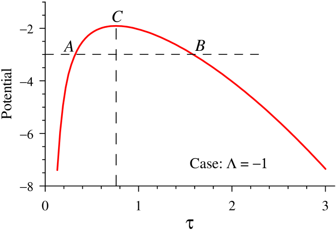
Figure 10: Perspective view of the potential $\mathcal{U}(\tau)$ with a negative $\Lambda$.

As one sees from Fig. LABEL:Bulbous, depending on the integration constant and initial value of $\tau$, the mode of evolution can be both finite and exponential. For the integration constant being at the level $AB$ in Fig. LABEL:Bulbous (here it is $-3$), with $\tau_{0}\in(0,\tau_{A})$ the evolution of $\tau$ finite and similar to one in Fig. 2 corresponding to $E=1$, whereas, for $\tau_{0}>\tau_{B}$ we have $\tau$ that is expanding exponentially. In case of $E$ being at the same level with point $M$ we have the similar picture of evolution, but in this case once $\tau$ reaches point $\tau_{M}$, the process of evolution would come to a halt. Thus we conclude that for a trigonometric interaction term the system even with a negative $\Lambda$ admits non-exponential mode of evolution.

To investigate the dominant energy condition let us write the components of energy-momentum tensor. For simplicity we set $C_{0}=1$ and in term of $S$ for energy density we write

$$T_{0}^{0}=mS+\frac{S^{2}}{2(1+\lambda\sin S)}+\varepsilon_{0}S^{1+\zeta}.$$ (3.25)

Since $\tau$ is a positive quantity, $S$ is positive as well. As one sees from (3.25) for any positive value of $S$ and $\lambda<1$ energy density is always positive definite and proportional to $S^{2}$. Since $S=1/\tau$, it means that $T_{0}^{0}$ has its maximum as $\tau\to 0$ and tends to zero as $\tau\to\infty$.

On the For the pressure components we have

$$T_{1}^{1}=T_{2}^{2}=T_{3}^{3}=\frac{\lambda S^{3}\cos S}{2(1+\lambda\sin S)^{2}}-\frac{S^{2}}{2(1+\lambda\sin S)}-\varepsilon_{0}\zeta S^{1+\zeta}.$$ (3.26)

As one sees, for a $\lambda<1$ $T_{1}^{1}$ may both positive or negative depending on the sign of $\cos S$. Moreover, its maximum value is proportional to $S^{3}$. Thus, in case of $F=\sin S$ for all possible values of $\zeta$ and $\lambda$ (necessarily nontrivial) there exists intervals $(S_{n},S_{n+1})$ such that for $S\in(S_{n},S_{n+1})$ the inequality $T_{0}^{0}<T_{1}^{1}$ takes place as it is shown in Fig. LABEL:Section. Therefore we conclude that the regular solutions obtained in this case results in broken dominant energy condition.

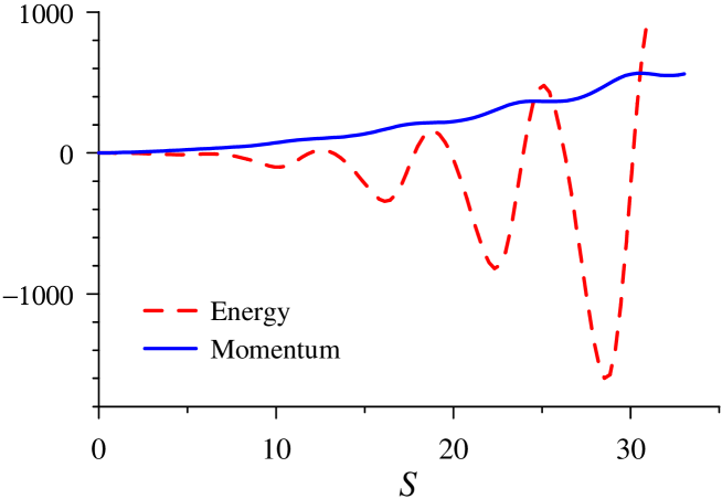
Figure 11: Perspective view of $T_{0}^{0}$ and $T_{1}^{1}$.

4 Conclusion

Within the framework of the simplest model of interacting spinor and scalar fields it is shown that the $\Lambda$ term plays very important role in BI cosmology. In particular, it invokes oscillations in the model which is not the case when $\Lambda$ term remains absent. For a non-positive $\Lambda$ we find an universe expanding exponentially, hence the initial anisotropy of the model quickly dies away, whereas for a positive $\Lambda$ with the corresponding choice of integration constant ${\mathcal{E}}$ one finds the oscillatory mode of expansion of the universe. In this case it is possible to construct solutions those are always regular. It should be emphasized that if the spinor field nonlinearity is generated by self-action the regularity of the solutions obtained results in the violation of the dominant energy condition of Penrose-Hawking theorem sahaprd , whereas in the case considered here, when the spinor field nonlinearity is induced by the scalar one, regular solutions can be obtained even without breaking the aforementioned condition. It should be noted that the dominant energy condition holds for $F$ being the power function of $I$ or $J$, whereas it is not the case when $F$ is given as a trigonometric function of its arguments. Note that in presence of $\Lambda$-term the role of other parameters such as order of nonlinearity $n$, perfect fluid parameter $\zeta$ and spinor mass in the evolution process are rather local, while the global process are totally determined by the $\Lambda$-term, e.g., for a positive $\Lambda$ we have always oscillatory mode, while for a negative $\Lambda$ solutions are generally inflation-like though for some special choices of problem parameters the oscillatory mode of evolution can be attained.

- (1) D. Ivanenko, Phys. Zs. Sowjetunion 13, 141 (1938).
- (2) D. Ivanenko, Soviet Physics Uspekhi 32, 149 (1947).
- (3) V. Rodichev, Soviet Physics JETP 13, 1029 (1961).
- (4) H. Weyl, Physical Review 77, 699 (1950).
- (5) R. Finkelstein, R. LeLevier and M. Ruderman, Physical Review 83, 326 (1951).
- (6) C. Armendriz-Picn and P.B. Greene, hep-th/0301129.
- (7) C.W. Misner, Astrophysical Journal 151, 431 (1968).
- (8) Ya.B. Zel’dovich, Letters to Journal of Experimental and Theoretical Physics 12, 443 (1970).
- (9) V.N. Lukash and A.A. Starobinsky, Journal of Experimental and Theoretical Physics 66, 1515 (1974).
- (10) V.N. Lukash, I.D. Novikov, A.A. Starobinsky, and Ya.B. Zel’dovich, Nuovo Cimento B 35, 293 (1976).
- (11) Hu B.L. and Parker L., Physical Review D 17, 933 (1978).
- (12) V.A. Belinskii, I.M. Khalatnikov and E.M. Lifshitz, Advances in Physics 19, 525 (1970).
- (13) K.C. Jacobs, Astrophysical Journal 153, 661 (1968).
- (14) B. Saha and G.N. Shikin, Journal Mathematical Physics 38, 5305 (1997).
- (15) Bijan Saha, Physical Review D 64, 123501 (2001).
- (16) B. Saha and G.N. Shikin, General Relativity and Gravitation 29, 1099 (1997).
- (17) Bijan Saha, Modern Physics Letters A 16, 1287 (2001).
- (18) V.A. Belinskii and I.M. Khalatnikov, Landau Institute Report, 1976.
- (19) Henneaux M., Physical Review D 18, 969 (1980).
- (20) Henneaux M., Ann. Inst. Henri Poincar, Sect. A 34, 329 (1981).
- (21) T.W.B. Kibble, J. Math. Phys. 2, 212 (1961).
- (22) V.B. Berestetski, E.M. Lifshitz and L.P. Pitaevski, Quantum Electrodynamics (Nauka, Moscow, 1989).
- (23) V.A. Zhelnorovich, Spinor theory and its application in physics and mechanics (Nauka, Moscow, 1982).
- (24) D. Brill and J. Wheeler, Review of Modern Physics 29, 465 (1957).
- (25) E Kamke, Differentialgleichungen losungsmethoden und losungen (Leipzig, 1957).
- (26) Ya.B. Zeldovich and I.D. Novikov, Structure and evolution of the Universe (Nauka, Moscow, 1975).
- (27) S.W. Hawking and R. Penrose, Proceedings of the Royal Society of London. Mathematical and physical sciences 314, 529 (1970).
- (28) W. Heisenberg, Introduction to the unified field theory of elementary particles (Interscience Publ., London, 1966).
- (29) L.D. Landau and E.M. Lishitz, Course of theoretical physics, vol. 1, Mechanics (Oxford: Butterworth-Heinemann, 1976).