A criterion for bubble formation
in de Sitter universe

Abstract

The influence of the shape of scalar field potential on the outcome of vacuum decay in de Sitter universe is studied. Sufficient condition for vacuum decay via bubble formation, described by Coleman - de Luccia instanton, is revisited and necessary condition is found. Both conditions require that the curvature of the potential is greater than 4 $\times$ (Hubble constant)², but while the sufficient condition states that this inequality is to be valid at the top of the barrier, the necessary condition requires that it holds at least somewhere throughout the barrier. The conditions leave a ’grey zone’ in parameter space, which however seems to be forbidden for quartic potential as well as for quadratic potential with a narrow peak proposed by Linde in the context of open inflation.

1 Introduction

The concept of vacuum decay via formation of rapidly expanding bubbles was introduced by Coleman [1], and its general relativistic extension, with bubbles created in de Sitter universe, was developed by Coleman and de Luccia [2]. The process was an important ingredient of old inflation [3], and it emerged again in the scenario of open inflation [4, 5, 6]. An alternative mode of vacuum decay, applying presumably to the initial stage of new inflation [7, 8], was proposed by Hawking and Moss [9]. In this mode, the transition should occur in the whole universe at once; however, as seen from elementary considerations and confirmed by stochastic theory [10], this must not be taken too literally. In fact, homogeneous transition takes place only inside the event horizon where the metric assumes de Sitter form due to cosmological no-hair theorem. Each mode of vacuum decay is described by corresponding instanton: the decay in a bubble by Coleman - de Luccia instanton (CdL instanton), and the decay in a horizon-size domain by Hawking - Moss instanton (HM instanton). CdL instanton is a squeezed 4-sphere with an O(4) configuration of scalar field living on it which contains a 4D version of the bubble; HM instanton is a round 4-sphere filled with scalar field which is located at the top of the barrier everywhere. It has been argued [9, 11] that CdL instanton exists only if the curvature of the potential in the false vacuum is greater than 4 $\times$ (Hubble constant)². The radius of the 4-sphere equals approximately (Hubble constant)^-1 and the width of the bubble wall equals approximately (curvature of the potential)^-1/2, thus the criterion just states that the bubble must fit into the sphere. If it does not, vacuum decays via HM instanton which exists regardless of the shape of the potential. The criterion for the existence of CdL instanton has been formulated as approximate, valid only for potentials of the kind used in new inflation. However, it might be expected that this criterion, or some modification of it, holds for an arbitrary potential as well. In this article we propose a candidate for a generally valid criterion and demonstrate its effectiveness on two examples.

2 Sufficient condition

CdL instanton is a nontrivial finite-action O(4) solution of Eucleidean equations for coupled gravitational and scalar field, obtained in a theory with an effective potential containing true vacuum (global minimum in which it equals zero) and false vacuum (local minimum) separated from the true vacuum by a finite potential barrier. It is given by two functions $\phi(\rho)$ and $a(\rho)$, where $\phi$ is the scalar field, $a$ is the radius of 3-spheres of homogenity determined from the circumference and $\rho$ is the radius of 3-spheres of homogenity measured from the centre. Denote the effective potential $V$. Functions $\phi$ and $a$ obey the equations

$$\ddot{\phi}+\frac{3\dot{a}}{a}\ \dot{\phi}=V^{\prime},\ \ \dot{a}^{2}=\frac{8\pi}{3}\left(\frac{1}{2}\dot{\phi}^{2}-V\right)\ a^{2}+1,$$ (1)

where the dot denotes differentiation with respect to $\rho$ and the prime denotes differentiation with respect to $\phi$. (Throughout the paper, we use ’Mr. Tompkins’ system of units in which $c=G=\hbar=1$.) Let us write down also the second order equation for $a$ which is often helpful in general considerations, and is more appropriate for numerical calculations than the first order equation. It reads

$$\ddot{a}=-\frac{8\pi}{3}\left(\dot{\phi}^{2}+V\right)\ a.$$ (2)

The function $a$ is concave everywhere and starts from zero at $\rho=0$ (the second possibility, namely that it is infinite there, is excluded by concavity), thus it must first increase and then decrease until it reaches zero at some $\rho_{f}$. To ensure the finitness of action we require that the solution is finite both at $\rho=0$ and $\rho=\rho_{f}$. The corresponding boundary conditions are

$$a(0)=\dot{\phi}(0)=\dot{\phi}(\rho_{f})=0.$$ (3)

Denote $\phi_{i}$ and $\phi_{f}$ the initial and final value of $\phi$. If we choose $\phi_{i}$ at random, $\phi_{f}$ will most probably be infinite, with the function $\phi$ either increasing or decreasing logaritmically as $\rho$ approaches $\rho_{f}$. Instanton solutions, if any, exist only for discrete $\phi_{i}$’s. Function $\phi$ for an instanton solution is confined to the barrier, and from its behaviour in the vicinity of $\rho=0$ and $\rho=\rho_{f}$ it is easily seen that it cannot be located on one side of the barrier only. Indeed, it equals approximately $\phi_{i}+V^{\prime}_{i}\rho^{2}/8$ for $\rho\sim 0$ and $\phi_{f}+V^{\prime}_{f}\ (\rho_{f}-\rho)^{2}/8$ for $\rho\sim\rho_{f}$, hence if it starts and ends, say, on the near side of the barrier where $V^{\prime}>0$, it rises at the beginning and falls at the end. Consequently, there must be at least one turning point between $\rho=0$ and $\rho=\rho_{f}$, and this turning point, or first of these turning points if more of them exist, must be located on the far side of the barrier since $\dot{\phi}=0$ and $\ddot{\phi}>0$ there. As a result, the value $\phi_{top}$ at which $V$ reaches maximum is crossed by the function $\phi$ at least once. If the total number of crossings is $l$, one may call the solution ’CdL instanton of $l$th order’. Equation for the function $\phi$ may be viewed as equation of motion of a pointlike particle in the potential $-V$, with time-dependent friction coefficient $3\dot{a}/a$. The energy of the particle

$$E=\frac{1}{2}\dot{\phi}^{2}-V$$ (4)

obeys

$$\dot{E}=-\frac{3\dot{a}}{a}\ \dot{\phi}^{2},$$ (5)

thus it decreases in friction regime, when $a$ increases from zero to some maximum value, and increases in antifriction regime, when $a$ returns to zero. For instanton solutions, the curve $E(\phi)$ starts and ends on a wall of the barrier (which becomes a well when we pass to the flipped potential), crossing the barrier $l$ times if the instanton is of order $l$. For non-instanton solutions, the curve looks the same except that it escapes to infinity at the end. In the vicinity of an instanton solution there are non-instanton ones which either bounce back to infinity below the point where the instanton solution stops, or slip forward to infinity above it, see fig. 1. The former solutions may be called undershootings and the latter overshootings.

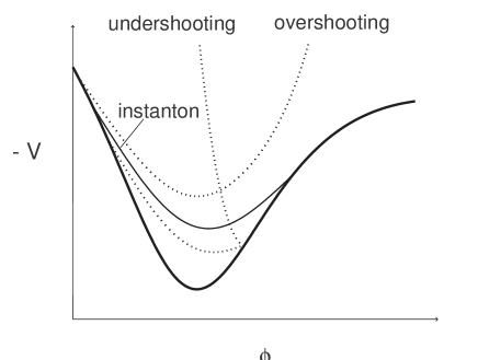
Figure 1: Energy curves

Continuity implies that in order to ’disentangle’ the last turning point of a non-instanton solution, we must pass through a sequence containing necessarily an instanton solution having one turning point less. Furthermore, from a slight extension of the original Coleman argument valid for an instanton in flat space [1] it follows that solutions starting sufficiently near to the true vacuum are always ’short’ overshootings escaping to infinity close to the starting point [11]. Putting this together we see that over an instanton of $l$th order there must be a tower of instantons of orders $l-1,\ l-2,\ \ldots$, possibly containing more instantons of the same order. No matter how numerous the instantons are, only that with the least action is of physical relevance. Presumably this is the instanton of first order, at least for ’well-behaved’ potentials for which the complete tower of instantons contains one representative of each order only and the starting point moves away from $\phi_{top}$ as the order of instanton decreases. Introduce now a limit solution which is, at least half-and-half, shrinked to the top of the barrier, with $\phi=\phi_{top}$ inserted into the equation for $a$ and the linearized expression for $V^{\prime}$ inserted into the equation for $\phi$. From the former equation we find $a=H^{-1}\sin(H\rho)$, where $H=\sqrt{8\pi V_{top}/3}$, and inserting this into the latter equation we obtain

$$\Delta\ddot{\phi}+3H\ \mbox{cotan}(H\rho)\ \Delta\dot{\phi}=-\mu^{2}\Delta\phi,$$ (6)

where $\Delta\phi=\phi-\phi_{top}$ and $\mu=\sqrt{-V_{top}^{\prime\prime}}$. The 4D space is a 4-sphere with radius $H^{-1}$ and the equation for $\phi$ is the eigenvalue equation for Laplace operator on a 4-sphere. The equation assumes standard form if we pass from $\Delta\phi$ and $\rho$ to $x=\Delta\phi/\Delta\phi_{i}$ and $\varphi=H\rho$, and introduce $\lambda=\mu^{2}/H^{2}$. Finite solutions exist only for $\lambda_{l}=l\ (l+3)=0,\ 4,\ 10,\ldots$ and are of the form

$$x_{l}=1,\ \cos\varphi,\ \frac{1}{4}(5\cos^{2}\varphi-1),\ldots$$ (7)

Consider a 1-parameter class of potentials with $\lambda$ increasing from zero to infinity. For $\lambda=\lambda_{l}$ we have ’zero instanton of $l$th order’ located at the top of the barrier (that is, dispersed infinitesimally around $\phi_{top}$); for other values of $\lambda$, we have a non-instanton limit solution located at the top of the barrier on one side and escaping to $\phi=+\infty$ or $-\infty$ on the other side. Note that this soltion has a different asymptotics at $\rho\to\rho_{f}$ than the true solution, namely power-like instead of logarithmic, thus it must be cut and matched to the true asymptotic solution at some $\rho$ to obtain a correct approximative solution. For $\lambda$ between $\lambda_{l}$ and $\lambda_{l+1}$, the limit solution has the same number of turning points as $x_{l+1}$. Indeed, when $x_{l+1}$ deforms to $x$ with a bit smaller $\lambda$, it does not turn to the opposite direction, see appendix A, and when one $x$ deforms to another, turning points may not vanish or arise since $x$ may not have a maximum below zero or a minimum above zero, see the argument against the localization of an instanton on one side of the barrier. This implies, by the ’disentanglement’ argument, that for $\lambda$ between $\lambda_{l}$ and $\lambda_{l+1}$ an instanton of $l$th order must exist somewhere at a finite distance from the top of the barrier, and consequently, that CdL instanton necessarily exists for $\lambda>\lambda_{1}$. Inserting for $\lambda$ and $\lambda_{1}$ we obtain $\mu^{2}>4H^{2}$, or

$$-V^{\prime\prime}>\frac{32\pi}{3}V\ \ \mbox{at}\ \ \phi=\phi_{top}.$$ (8)

3 Necessary condition

The condition from the previous section has been proposed in [9] and discussed [11] in the context of new inflation, for potentials with a tiny barrier above a plateau with an almost zero slope. In fact, the inequality in the cited articles differs from ours: it reads $\mu^{2}>4H^{2}$, too, but with $H$ defined as $\sqrt{8\pi V_{f.v.}/3}$, where $V_{f.v.}$ is the value of $V$ in false vacuum. However, the considerations in both articles are approximative only, neclecting the effect of small variations of the potential throughout the barrier on the form of the 4D space, thus the difference between $V_{f.v.}$ and $V_{top}$ plays no role in them. In the first article it is claimed, with a brief comment referring to the size of the bubble filled with true vacuum in flat space, that the validity of $\mu^{2}>4H^{2}$ is necessary and sufficient for the existence of CdL instanton; in the second article the necessary condition is supplemented by the assumption that $V^{\prime\prime}$ decreases monotonously as one approaches $\phi_{top}$ from the side of false vacuum (actually, the authors require that $V^{\prime\prime}$ increases, but this is obviously an oversight) and the proof of both necessary and sufficient condition is sketched. In all considerations, the 4D space is supposed to have the metric of a 4-sphere. As we have seen, the sufficient condition survives, with redefined $H$, also in a theory without this simplification; and a natural question arises whether this is possibly true about the necessary condition as well. If it were, it would provide us with a simple algebraic criterion for the existence of CdL instantons, applicable on a wide class of potentials including quartic. Unfortunately, we were not able to extend the argument of [11] to the exact theory. (In fact, the argument seems rather handwaving even in the approximation considered there.) We propose instead a condition which is weaker in practical respect, but it still rules out a considerable portion of parameter space. In the next section it will turn out that the condition $\mu^{2}>4H^{2}$ is apparently necessary and sufficient at the same time for a rather wide class of potentials, therefore it is perhaps useful to see why this cannot be the case for any potential. An obvious counter-example is a properly smoothed-out ’safe’ potential: one takes a potential obeying the inequality $\mu^{2}>4H^{2}$ with large enough margin to allow for an instanton whose energy is high above $-V_{top}$, and smoothes out the neighbourhood of $V_{top}$ so that the inequality $\mu^{2}>4H^{2}$ will not be valid anymore. The constraint on $V^{\prime\prime}$ proposed in [11] is plausible at least in that that it rules out such construction. To obtain the condition we are seeking for, let us pass from the equations for $\phi$ and $a$ to the equation for $E$,

$$E^{\prime\prime}=8\pi(2E+3V)+\frac{E^{\prime}\left(\frac{2}{3}E^{\prime}+\frac{1}{2}V^{\prime}\right)}{E+V}.$$ (9)

Note that this equation is of second order, while the equation which one obtains from the system (1) by elimination method is of third order: we have traded one order of differential equation for allowing the equation to contain the argument of unknown function. The initial conditions are

$$E_{i}=V_{i},\ \ E_{i}^{\prime}=-\frac{3}{4}V_{i}^{\prime}$$ (10)

and the initial value of the second derivative of $E$ is

$$E_{i}^{\prime\prime}=\frac{8\pi}{3}V_{i}-\frac{1}{2}V_{i}^{\prime\prime}.$$ (11)

If we denote $\delta E=E+3V/4$ and ${\cal V}=8\pi V/3+V^{\prime\prime}/4$, from the expressions for $E_{i}^{\prime}$ and $E_{i}^{\prime\prime}$ we find that the function $\delta E^{\prime}$ equals zero and its derivative equals ${\cal V}_{i}$ at $\phi=\phi_{i}$. For an instanton we have, in addition to the two conditions at $\phi=\phi_{i}$, similar two conditions at $\phi=\phi_{f}$; thus the function $\delta E^{\prime}$ equals zero and its derivative equals ${\cal V}_{f}$ there. Furthermore, if $\delta E^{\prime}$ approaches zero outside the points $\phi_{i}$ and $\phi_{f}$, its derivative tends to $8\pi(2E+3V)+3V^{\prime\prime}/4$, which is greater than $8\pi V+3V^{\prime\prime}/4=3{\cal V}$. Suppose ${\cal V}>0$ throughout the barrier. In such potential, $\delta E^{\prime}$ for an instanton rises above zero at the beginning and it should return to zero from below at the end, hence it should cross zero from above somewhere in between; however, if it comes close to zero at some point, its tangent becomes positive and it bounces back. As a result, an instanton may exist only if there is a place somewhere inside the barrier where the inequality ${\cal V}>0$ is violated, that is if

$$-V^{\prime\prime}>\frac{32\pi}{3}V\ \ \mbox{at some}\ \ \phi\ \ \mbox{inside the barier}.$$ (12)

4 Examples

The first example we shall discuss is quartic potential

$$V=\frac{1}{2}\phi^{2}-\frac{1}{3}\delta\phi^{3}+\frac{1}{4}\lambda\phi^{4},$$ (13)

with two parameters $\delta$ and $\lambda$ which are both supposed to be positive. Usually, the first term is multiplied by $m^{2}$, so that $V$ contains one more parameter, the mass of the scalar field $m$. However, this parameter may be removed from the theory by the rescalings $a\to a/m$ and $\rho\to\rho/m$ in the equations for $\phi$ and $a$, supplemented by the rescalings $\delta\to m^{2}\delta$ and $\lambda\to m^{2}\lambda$ in the expression for $V$. The quartic potential is of the type we are interested in in a rather narrow range of parameters, for $\delta$ ranging from $\delta_{m}=2\sqrt{\lambda}$ to $\delta_{M}=3\sqrt{\lambda/2}\doteq 1.06\delta_{m}$. This is discussed, along with other properties of $V$, in appendix B. In what follows, we use instead of $\delta$ its linear transform

$$x=\frac{\delta-\delta_{m}}{\delta_{M}-\delta_{m}},$$ (14)

rearranging the parameter space into a half-infinite strip of unit width. Let us investigate the possibility of the existence of CdL instanton in quartic potential. Denote $\lambda_{N}$ and $\lambda_{S}$ the limit values of $\lambda$ at which the necessary and sufficient condition for the existence of CdL instanton are valid. The two $\lambda$’s correspond to two particular configurations of the curves $\hat{V}=32\pi V/3$ and $-V^{\prime\prime}$: at $\lambda_{S}$ the latter curve crosses the former at its peak, and at $\lambda_{N}$ the latter curve becomes tangent to the former at some point, lying below it everywhere outside that point. Denote, furthermore, $\phi_{S}$ the value of $\phi_{top}$ for $\lambda=\lambda_{S}$. In appendix B, the dependence of $\lambda_{S}$ and $\phi_{S}$ on $x$ is given analytically, see equations (B-2), (B-3) and (B-4), and the dependence of $\lambda_{N}$ on $x$ is expressed in parametric form, see equations (B-5) and the discussion below. The first two functions, together with allowed regions of $\lambda$ and $\phi_{top}$, are depicted in fig. 2.

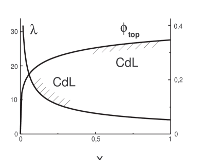
Figure 2: Allowed regions for CdL instanton in quartic potential

The allowed regions are shaded at the boundary and denoted by the corresponding variable, and two sets of tic labels are given at the vertical axes, those referring to $\lambda$ on the left and those referring to $\phi_{top}$ on the right. As we can see, the values of $\lambda$ are bounded from below while the values of $\phi_{top}$ are bounded from above. The domain $\lambda_{N}<\lambda<\lambda_{S}$, with contour lines characterizing the behaviour of the solutions of instanton equations, is depicted in fig. 3.

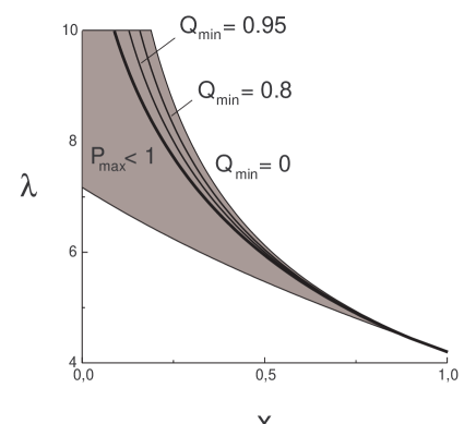
Figure 3: Topography of ’grey zone’ for quartic potential

This is the ’grey zone’ of the parameter space in which we cannot decide whether the potential admits an instanton or not but numerically. Sample calculations reveal no instanton solutions there, but this of course does not rule out the possibility that they exist. The character of the solutions may be explored systematically by defining an appropriate global characteristic of the solutions and drawing its contour lines. For a potential from the ’grey zone’, the curve $-V^{\prime\prime}$ reaches out of the curve $\hat{V}$ only in some interval $(\phi_{A},\phi_{B})$ between $\phi_{top}$ and the true vacuum at $\phi=0$, shrinking from maximum size to a point as $\lambda$ decreases from $\lambda_{S}$ to $\lambda_{N}$. Consider solutions to the instanton equations starting on the true-vacuum side of $\phi_{top}$ for which the function $\delta E^{\prime}$ is negative somewhere; these are all solutions starting in the interval $(\phi_{A},\phi_{B})$, since for them the function $\delta E^{\prime}$ becomes negative immediately after the start, and possibly some solutions starting before $\phi_{A}$, since for them this function may become negative later. If the potential does not admit instantons, the function $\delta E^{\prime}$ crosses zero again at some $\phi_{lim}$ and escapes to infinity after. Since the solutions do not come to a halt at $\phi_{lim}$, the quantity $\Delta E=E+V$ is positive there, $\Delta E_{lim}>0$. If, on the other hand, the potential does admit instantons, they belong to the class of solutions in question; and among them there is an instanton of first order for which the function $\delta E^{\prime}$ stops after returning to zero on the far side of $\phi_{top}$, so that $\phi_{lim}>\phi_{top}$ and $\Delta E_{lim}=0$. Define

$$P=\frac{\phi_{lim}}{\phi_{top}},\ \ Q=\left\{\begin{array}[]{l}\Delta E_{lim}/(E_{lim}+V_{top})\ \mbox{if}\ P\geq 1\\ 1\ \mbox{if}\ P<1\\ \end{array}.\right.$$ (15)

As follows from previous discussion, for potentials admitting no instantons $P_{max}$ may be $>1$ as well as $\leq 1$ and $Q_{min}$ is necessarily positive, while for potentials that do admit instantons $P_{max}>1$ and $Q_{min}=0$. By continuity argument, if we are close enough to a domain in parameter space in which instantons are allowed, $P_{max}$ must exceed 1, and as we approach the bordeline of this domain from outside, $Q_{min}$ must decrease from some moment on until it reaches zero at the borderline. In fig. 3, the thick line corresponds to $P_{max}=Q_{min}=1$ and the thin lines above it, in the strip where $P_{max}>1$, correspond to values of $Q_{min}$ given next to them. The form of the lines strongly suggests that as we cross the strip, $Q_{min}$ decreases from 1 to 0 monotonously, hence no instantons occur in the ’grey zone’. Quartic potential may be used to demonstrate how difficult it is to obtain open inflation in a ’natural’ way. A single-field open inflation requires an instanton solution whose limit value of $\phi$ on the true-vacuum side of $\phi_{top}$ is greater than about 3; and from a simple qualitative analysis it follows [5, 6] that for quartic potential no such solution exists. Our computation confirms this. Indeed, the allowed region of $\phi_{top}$ in fig. 2 is located deeply under the line $\phi_{top}=3$, and as long as one regards the whole ’grey zone’ as forbidden for the instantons, this region contains all admissible values of $\phi_{top}$. Consequently, the values of $\phi_{top}$ for potentials that do admit instantons are significantly less than 3, and the same is true of any value of $\phi$ that may be reached by an instanton solution on the true-vacuum side of $\phi_{top}$. Let us proceed to our second example, a superposition of quadratic and Breit - Wigner type potential

$$V=\frac{1}{2}\phi^{2}\left[1+\frac{\alpha^{2}}{\beta^{2}+(\phi-v)^{2}}\right].$$ (16)

Again, we have scaled away the mass $m$. This potential has been introduced by Linde in his toy model of open inflation [6], with the mass set to the value $m\simeq 10^{-6}$ in order to get the proper size of density fluctuations. For $\beta$ sufficiently small, $V$ has a peak centered near $\phi=v$ with the width $\beta$ and relative overheight $k=\alpha^{2}/\beta^{2}$. To illustrate the properties of such potential, the values $v=3.5$, $k=0.5$ and $\beta=0.1$ have been chosen in [6]. To observe the constraint on the potential coming from the scenario of open inflation (provided the peak is narrow, which is necessarily the case if an instanton is to occur at all), one has to take $v\gtrsim 3$; and a value at the lower end of this range has to be chosen if one wishes to obtain the cosmological parameter $\Omega$ not too close to 1. Denote $k_{N}$ and $k_{S}$ the limit values of $k$ for which the necessary and sufficient condition of the existence of CdL instanton is fulfilled. In appendix C it is shown that if $v$ is large enough to allow for open inflation, these quantities approximately coincide, and they increase from zero to infinity as $\beta$ increases from zero to $B=\sqrt{3/(16\pi)}\doteq 0.24$, switching from linear to quadratic dependence on $\beta$ near $b=B^{2}/v$, $b\doteq 0.017$ for $v=3.5$. The corresponding formulas are summarized in equation (C-2). Between $k_{S}$ and $k_{N}$ there should be a ’grey zone’. In the first approximation this zone is absent; however, its size may be deduced from the corrections to $k_{S}$ and $k_{N}$, see equations (C-3) and (C-4) for $\beta\gg b$ and equation (C-5) for $\beta\ll b$. The zone turns out to be quite narrow; for example, for values of $v$ and $\beta$ used in [6] one obtains $k_{S}=0.23$ and $k_{N}=0.20$. The possible existence of CdL instanton in the ’grey zone’ could now be investigated by drawing similar contour lines as for quartic potential. However, for $\beta\gg b$ one may determine the character of the ’grey zone’ on the basis of the results for quartic potential only. The point is that in this part of ’grey zone’ the curve $-V^{\prime\prime}$ exceeds the curve $\hat{V}$ only in a tiny interval of $\phi$ close to $\phi_{top}$, like for quartic potential with $x$ close to 1, and both curves may be approximated by inverted parabolas throughout this interval, again like for quartic potential with $x$ close to 1. Consequently, since the interval under consideration plus a small adjacent region is all what is relevant for the problem of the existence of CdL instanton, and since all the ’grey zone’ for quartic potential is presumably forbidden, the ’grey zone’ for Linde potential with $\beta\gg b$ should be forbidden, too. On the other hand, for $\beta\ll b$ the zone is so narrow that it is of no relevance at all, in view of the uncertainties in the form of the potential in any not-exactly-toy model.

5 Conclusion

We have shown that if the inequality $-V^{\prime\prime}>32\pi V/3$ holds at the top of the barrier, the potential admits CdL instanton, and if this inequality is valid at least somewhere throughout the barrier, the potential may admit CdL instanton. Otherwise only HM instanton exists. (HM instanton is by definition trivial solution to equations (1), which in our notations reads $\phi=\phi_{top}$ and $a=H^{-1}\sin(H\rho)$.) The necessary condition for the existence of CdL instanton does not restrict the form of the potential in advance, like the constraint on $V^{\prime\prime}$ in [11]. However, this is achieved at the price that the condition is weaker than the sufficient condition for any but very specific potentials, not allowing for the algebraic solution of the problem even in the simplest case of quartic potential. To obtain a sharp borderline between the regions in parameter space in which vacuum decays in the way described by CdL and HM instanton, one may use the method of contour lines outlined in section 4. As we have seen, by applying this method on quartic potential one finds that the sufficient condition is most probably also necessary, thus the existence of CdL instanton depends uniquely on the form of the potential at the top of the barrier. The same is true, at least for potentials whose barrier is not too narrow, about Linde potential. An open question remains what is the largest class of potentials with this property.

Acknowledgements. This work was supported by the grant VEGA 1/0250/03.

Appendix A Unbounded solutions to the eigenvalue problem

The eigenvalue equation

$$\ddot{x}+3\ \mbox{cotan}\varphi\ \dot{x}+\lambda x=0,$$ (A-1)

where the dot denotes differentiation with respect to $\varphi$, transforms under the substitution $z=\sin^{2}(\varphi/2)$ into an equation for (nondegenerate) hypergeometric function

$$z(1-z)\ x^{\prime\prime}+2(1-2z)\ x^{\prime}+\lambda x=0,$$ (A-2)

where the prime denotes differentiation with respect to $z$. This yields

$$x=F\left(\frac{3}{2}+\Lambda,\ \frac{3}{2}-\Lambda,\ 2;\ \sin^{2}\frac{\varphi}{2}\right),\ \ \Lambda\equiv\sqrt{\frac{9}{4}+\lambda},$$ (A-3)

and with the help of the identity

$$F(a,\ b,\ c;\ z)=(1-z)^{c-a-b}F(c-a,\ c-b,\ c;\ z)$$

we find that $x$ diverges quadratically as $\varphi$ approaches $\pi$, $x\simeq k(\pi-\varphi)^{-2}$, with the constant of proportionality

$$k=4F\left(\frac{1}{2}+\Lambda,\ \frac{1}{2}-\Lambda,\ 2;\ 1\right)=-\frac{4\cos(\Lambda\pi)}{(2+\lambda)\pi}.$$ (A-4)

The function $k(\lambda)$ oscillates around zero with nods at $\lambda=\lambda_{l}$ and is negative between $\lambda_{0}$ and $\lambda_{1}$. Consequently, if $\lambda$ is from the interval ($\lambda_{l},\ \lambda_{l+1})$, $x$ diverges to $-\infty$ and $+\infty$ for even and odd $l$ respectively, and since $x_{l+1}$ decreases when approaching its endpoint for even $l$ and increases for odd $l$, no turning point arises when $x$ disconnects from $x_{l+1}$.

Appendix B Properties of quartic potential

Quartic potential has a minimum equal to zero at $\phi=0$ and for $\delta>\delta_{m}=2\sqrt{\lambda}$ it has another two extremes at

$$\phi_{\pm}=\frac{\delta}{2\lambda}\pm\sqrt{\frac{\delta^{2}}{4\lambda^{2}}-\frac{1}{\lambda}};$$ (B-1)

furthermore, for $\delta<\delta_{M}=3\sqrt{\lambda/2}$ it is nonnegative everywhere, with only zero at $\phi=0$. Consequently, for $\delta_{m}<\delta<\delta_{M}$ the potential has the desired form, with true vacuum at $\phi=0$, false vacuum at $\phi=\phi_{+}$ and the top of the barrier at $\phi=\phi_{-}$. Let us compute $\lambda_{S}$ and $\phi_{S}$ for such potential. In present notations, $\lambda_{S}$ is given by the equation $\mu_{-}^{2}(\lambda_{S})=4H_{-}^{2}(\lambda_{S})$, where $H_{\pm}^{2}=8\pi V_{\pm}/3$ and $\mu_{\pm}^{2}=|V_{\pm}^{\prime\prime}|$, and $\phi_{S}$ equals $\phi_{-}(\lambda_{S})$. It holds

$$H_{\pm}^{2}=\frac{2\pi}{9\lambda}\frac{(1\pm X)(1\mp 3X)}{(1\mp X)^{2}},\ \ \mu_{\pm}^{2}=\frac{2X}{1\mp X},\ \ X\equiv\sqrt{1-\frac{4\lambda}{\delta^{2}}},$$

hence the equation for $\lambda_{S}$ yields

$$\lambda_{S}=\frac{4\pi}{9}\frac{(1-X)(1+3X)}{X(1+X)},$$ (B-2)

and if we express $\phi_{-}$ in terms of $\lambda$ and $X$ and exploit the above equation, we find

$$\phi_{S}=\frac{3}{2}\sqrt{\frac{X}{\pi(1+3X)}}.$$ (B-3)

The parameter $X$ depends on the parameter $x$, running from 0 to 1/3 as $x$ runs from 0 to 1,

$$X=\sqrt{1-\frac{1}{(1+\kappa x)^{2}}},\ \ \kappa\equiv\frac{\delta_{M}}{\delta_{m}}-1.$$ (B-4)

Let us proceed to $\lambda_{N}$. After the rescalings $\phi\to\phi/\sqrt{\lambda}$ and $\delta\to\sqrt{\lambda}\delta$ we have

$$\hat{V}=\frac{32\pi}{3\lambda}\phi^{2}\left(\frac{1}{2}-\frac{1}{3}\delta\phi+\frac{1}{4}\phi^{2}\right),\ \ -V^{\prime\prime}=-1+2\delta\phi-3\phi^{2},$$

so that if we change $\lambda$ leaving $\delta$ unchanged, the curve $-V^{\prime\prime}$ remains the same while the curve $\hat{V}$ scales by a factor inversely proportional to $\lambda$. Note that $\delta$ unchanged now means $x$ unchanged, too, since we have replaced $\delta$ by $\delta_{new}=\delta/\sqrt{\lambda}=2(1+\kappa x)$. The curves $-V^{\prime\prime}$ and $\hat{V}$ are both concave in the relevant interval in which $-V^{\prime\prime}$ exceeds zero; consequently, if $\lambda$ decreases from infinity to zero, so that $\hat{V}$ transforms from a segment on horizontal axis to an infinitely high peak, the part of $-V^{\prime\prime}$ reaching out of $\hat{V}$ shrinks from the whole curve $-V^{\prime\prime}$ in the interval of interest to a point, and then the two curves disconnect. As a result, for each $\delta$ we have unique $\lambda$ for which the curves $-V^{\prime\prime}$ and $\hat{V}$ are tangent, and since the former curve is located below the latter everywhere outside the oscular point, this $\lambda$ equals $\lambda_{N}$. Denote $\phi_{osc}$ the value of $\phi$ at the oscular point. For given $\delta$, $\phi_{osc}$ is determined, simultaneously with the critical $\lambda$ for which the oscular point exists, by the equations

$$\hat{V}_{osc}=-V_{osc}^{\prime\prime},\ \ \hat{V}_{osc}^{\prime}=-V_{osc}^{\prime\prime\prime},$$ (B-5)

and since the critical $\lambda$ is just $\lambda_{N}$, these equations may be viewed as a parametric definition of the function $\lambda_{N}(\delta)$. If we return from rescaled $\delta$ and $\phi$ to the original ones, the equations become linear in $\delta$ and $\lambda_{N}$ and solve trivially for any given $\phi_{osc}$. The only remaining task is to determine the limits of $\phi_{osc}$. The upper limit is reached at $x=1$ and coincides with the value of $\phi_{S}$ there, which is $\sqrt{3/(8\pi)}\doteq 0.35$; the lower limit is reached at $x=0$ and if we solve equations (B-5) numerically we find that it equals about 0.22.

Appendix C Properties of Linde potential

The extremes of Linde potential outside $\phi=0$ are given by

$$\left(1+x^{2}\right)^{2}=k\left(\frac{x}{\sigma}-1\right),$$ (C-1)

where $x=(\phi-v)/\beta$ and $\sigma=\beta/v$. Suppose $\sigma\ll 1$. (This assumption will be justified shortly). Two asymptotic regimes may be distinguished: if $k\gg\sigma$, the extremes are widely separated in the variable $x$, and if $k\doteq\kappa\sigma$, where $\kappa$ is a constant to be determined, the extremes are close to each other. In the former limit, the maximum is located close to zero at the point $x=(1+1/k)\sigma$ and the minimum is located far from 1 at the point $x=(k/\sigma)^{1/3}$; in the latter limit, both extremes are located close to the point $x=a$ at which they merge if $k\to 0$, $\sigma\to 0$ and $k/\sigma=\kappa$. By solving the equations $V^{\prime}=V^{\prime\prime}=0$ with $k\to 0$, $\sigma\to 0$ and finite $k/\sigma$ we obtain $a=1/\sqrt{3}$ and $\kappa=16/(3\sqrt{3})$. Let us find approximate expressions for $k_{S,N}$ as functions of $\beta$ and $v$. If $k_{S,N}$ are significantly greater than $\sigma$, they are both approximately given by the equation $-V_{0}^{\prime\prime}=\hat{V}_{0}$ where the index 0 refers to the point $x=0$. (By definition, $k_{S}$ and $k_{N}$ are given by the equation $-V^{\prime\prime}=\hat{V}$ at the points $x_{top}$ where $\hat{V}$ has maximum and $x_{osc}$ where $\hat{V}$ is tangent to $-V^{\prime\prime}$, however, both points are close to zero in the limit considered.) It holds $\hat{V}_{0}=16\pi v^{2}(1+k)/3$ and $-V_{0}^{\prime\prime}\doteq k/\sigma^{2}=kv^{2}/\beta^{2}$, hence $k_{S,N}$ are both approximately equal to $\beta^{2}/(B^{2}-\beta^{2})$, where $B=\sqrt{3/(16\pi)}$. The requirement that this expression is much greater than $\sigma$ yields $\beta\gg b=B^{2}/v$. Denote $k_{lim}$ the value of $k$ at which the two extremes of the potential outside $\phi=0$ merge, and under which the theory becomes inapplicable since no potential barrier exists. In the interval $\beta\ll b$ both $k_{S,N}$ must be close to $k_{lim}$ which equals approximately $k_{lim}^{(0)}=\kappa\sigma=\kappa\beta/v$ there; $k_{S}$ must be close to $k_{lim}$ since then the curve $-V^{\prime\prime}$ does not reach too high at the maximum of $\hat{V}$, being equal to zero at the inflex point of $\hat{V}$ if $k=k_{lim}$, and $k_{N}$ must be close to $k_{lim}$ (actually, it coicides with $k_{lim}$) since it may not exceed $k_{S}$. Putting this together we obtain

$$k_{S,N}\doteq\left\{\begin{array}[]{l}\beta^{2}/(B^{2}-\beta^{2})\ \mbox{if}\ \beta\gg b\\ \kappa\beta/v\ \mbox{if}\ \beta\ll b\\ \end{array}.\right.$$ (C-2)

The upper limit of $\beta$ is $B$, so that the upper limit of $\sigma$ is $B/v$; and since this number is less than 0.08 for $v>3$, our approximation works in the whole relevant range of parameters, if only as a qualitative estimate at its edge. Let us now discuss the corrections to $k_{S,N}$. In the interval $\beta\gg b$, we start from writing down the expansions of $\hat{V}$ and $-V^{\prime\prime}$ up to the second order in $x$,

$$\hat{V}=\frac{16\pi}{3}v^{2}(1+k)\left(1+2\sigma x-\frac{k}{1+k}x^{2}\right),\ \ -V^{\prime\prime}=\frac{k}{\sigma^{2}}\left(1+6\sigma x-6x^{2}\right)-1.$$

If we evaluate $k_{S}$ from the condition that the two parabolas intersect at the top of the first of them, and $k_{N}$ from the condition that the two parabolas are tangent, we obtain the previous expression with $B$ replaced by $B_{S,N}=B$ plus corrections of order $\sigma^{2}$. The shift of $B_{S}$ with respect to $B_{N}$ is

$$\Delta B=-\frac{9(1+k)(2+k)^{2}}{2k^{2}(6+5k)}\ \sigma^{2}B.$$ (C-3)

The curves $k_{S}$ and $k_{N}$ differ the most at $\beta$ not too close to $B$, where both $k_{S}$ and $k_{N}$ are small and the correction to $B_{S}$ dominates over the correction to $B_{N}$. Consequently, a good approximation of $k_{S}$ and $k_{N}$ is obtained for any admissible $\beta$ if one puts $B_{N}=B$, $B_{S}=B+\Delta B(k_{S})$; in this way the values of $k_{S}$ and $k_{N}$ cited in the text have been calculated. Furthermore, from the asymptotics of $\Delta B$ for $k\gg 1$ and $k\ll 1$ we find that, as we pass from $k_{N}$ to $k_{S}$, the upper limit of $\beta$ and the values of $k$ at $\beta\ll B$ become shifted by

$$\Delta\beta_{lim}=-\frac{9}{10}\frac{B^{3}}{v^{2}},\ \ \Delta k=\frac{6B^{2}}{v^{2}}.$$ (C-4)

In the interval $\beta\ll b$, we may evaluate $k_{S}$ from the equations $V_{top}^{\prime}=0$ and $-V_{top}^{\prime\prime}=\hat{V}_{top}$, assuming $x_{top}$ is close to $a$ and $k_{S}$ is close to $k_{lim}^{(0)}$. In this way we find that $k_{S}$ differs from $k_{lim}$ by a term proportional to $\beta^{3}$ only, while $k_{lim}$ itself differs from $k_{lim}^{(0)}$ by a term proportional to $\beta^{2}$. A similar procedure for $k_{N}$ yields nothing, which is understandable: as we shift the extremes to each other, the curve $\hat{V}$ relaxes to the parabola $16\pi\phi^{2}/3$, while retaining a ripple near $\phi=v$ whose slope varies rapidly; and because of this ripple, the curve $-V^{\prime\prime}$ acquires a sharp peak sticking out of $\hat{V}$. Consequently, $k_{N}$ in the interval $\beta\ll b$ coincides with $k_{lim}$ and $\Delta k$ with $k_{S}-k_{lim}$. Explicit calculation yields

$$\Delta k=\frac{1}{9}\frac{\kappa\beta^{3}}{vb^{2}}.$$ (C-5)

References

- [1] S. Coleman, Phys. Rev. D15, 2929 (1977).
- [2] S. Coleman and F. de Luccia, Phys. Rev. D21, 3305 (1980).
- [3] A. H. Guth, Phys. Rev. D23, 347 (1981).
- [4] M. Bucher, A. S. Goldhaber and N. Turok, Phys. Rev. D52, 3314 (1995).
- [5] A. D. Linde and A. Mezhlumian, Phys. Rev. D52, 6789 (1995).
- [6] A. D. Linde, Phys. Rev. D59, 023503 (1999).
- [7] A. Albrecht and P. J. Steinhardt, Phys. Rev. Lett. 48, 1220 (1982).
- [8] A. D. Linde, Phys. Lett. 108B, 389 (1982).
- [9] S. W. Hawking and I. G. Moss, Phys. Lett. 110B, 35 (1982).
- [10] A. D. Linde: Particle Physics and Inflationary Cosmology, Harwood, Chur, Switzerland (1990).
- [11] L. Jensen and P. J. Steinhardt, Nucl. Phys. B237, 176 (1984).