Copyright

by

Author Name Required !!!

2003

The Dissertation Committee for Author Name Required !!!

certifies that this is the approved version of the following dissertation:

Title Required !!!

Committee:

Philip J. Morrison, Supervisor

Matthew W. Choptuik, Supervisor

Richard Fitzpatrick

Richard A. Matzner

Paul R. Shapiro

To my mother…

Acknowledgments

First, I thank my supervisor, Matt Choptuik, for all that he has taught me, his refreshingly helpful manner, and the great patience he exhibited in working on this dissertation with me. It was truly a pleasure to work with him. In addition, I thank all my colleagues at UBC and the Center for Relativity at UT-Austin. I have learned much from the innumerable discussions with them and respect them all greatly. Especially, I wish to show my appreciation for the many helpful conversations I shared with Iñaki Olabarrieta, who served as a sounding board for many of my ideas.

I owe a great deal of gratitude to my mother, who always encouraged me to follow my passions in life and to achieve great things. Without her continuous support, I fear I would not have been able to come this far along in my studies. For all she has provided, I give my deepest love and appreciation to her. I also wish to thank my father for never ceasing to be interested in my endeavors, for fostering my interest in science, and for always being proud of his son.

For the past year I have been blessed with the love and emotional support from my dearest Somayeh. She has made this the happiest time of my life, and made writing this dissertation a much more delightful experience than it would have been without her.

Finally, I acknowledge financial support from the National Science Foundation grant PHY9722068 and and from the Natural Sciences and Engineering Research Council of Canada (NSERC). All the calculations referred to in this work were performed on the vn.physics.ubc.ca cluster at UBC funded by the Canadian Foundation for Innovation, NSERC and the Canadian Institute for Advanced Research.

Title Required !!!

Publication No.  

Author Name Required !!!, Ph.D.

The University of Texas at Austin, 2003

Supervisors: Philip J. Morrison Matthew W. Choptuik

We investigate the dynamics of self-gravitating, spherically-symmetric distributions of fluid through numerical means. In particular, systems involving neutron star models driven far from equilibrium in the strong-field regime of general relativity are studied. Hydrostatic solutions of Einstein’s equations using a stiff, polytropic equation of state are used for the stellar models. Even though the assumption of spherical symmetry simplifies Einstein’s equations a great deal, the hydrodynamic equations of motion coupled to the time-dependent geometry still represent a set of highly-coupled, nonlinear partial differential equations that can only be solved with computational methods. Further, many of the scenarios we examine involve highly-relativistic flows that require improvements upon previously published methods to simulate. Most importantly, with techniques such as those used and developed in this thesis, there is still considerable physics to be extracted from simulations of perfect fluid collapse, even in spherical symmetry. Here our particular focus is on the physical behavior of the coupled fluid-gravitational system at the threshold of black hole formation—so-called black hole critical phenomena.

To investigate such phenomena starting from conditions representing stable stars, we must drive the star far from its initial stable configuration. We use one of two different mechanisms to do this: setting the initial velocity profile of the star to be in-going, or collapsing a shell of massless scalar field onto the star. Both of these approaches give rise to a large range of dynamical scenarios that the star may follow. These scenarios have been extensively surveyed by using different initial star solutions, and by varying either the magnitude of the velocity profile or the amplitude of the scalar field pulse. In addition to illuminating the critical phenomena associated with the fluid collapse, the resulting phase diagram of possible outcomes provides an approximate picture of the stability of neutron stars to large, external perturbations that may occur in nature.

Black hole threshold, or critical, solutions, occur in in two varieties: Type I and Type II. Generically, a Type I solution is either static or periodic and exhibits a finite black hole mass at threshold, whereas a Type II solution is generally either discretely or continuously self-similar and characterized by infinitesimal black hole mass at threshold. We find both types of critical behavior in our space of star solutions. The Type I critical solutions we find are perturbed equilibrium solutions with masses slightly larger than their progenitors. In contrast, the Type II solutions are continuously self-similar solutions that strongly resemble those found previously in ultra-relativistic perfect fluids. The boundary between these two types of critical solutions is also discussed.

Table of Contents

toc

List of Tables

lot List of Figures

lof

Chapter 1 Introduction

The dynamics of compact gravitating objects out of equilibrium has always been a topic of much interest in astrophysics. Physical systems that fall under this subject include supernovae, failed supernovae such as hypernovae or collapsars, gamma-ray burst (GRB) progenitors, coalescing neutron star binary systems, accreting compact stars, and neutron stars that undergo sudden phase transitions, to only name a few. In many of these cases, a compact star is in such an excited state that it must catastrophically collapse and/or explode.

For those involving supernovae, the star has reached a non-equilibrium state either through accretion from a companion star (Type Ia), or—if sufficiently massive—by reaching the ultimate end in the thermonuclear cycles when fusion is no longer exothermic (Type II,Ib,Ic). In the former case, the unstable star is a white dwarf that has accreted past its Chandrasekhar limit, and consequently its electron degeneracy pressure is no longer sufficient to support it from gravitational collapse. The latter case, on the other hand, involves a star that has burned through successive elemental cores until an iron core has developed and can no longer support the star through thermonuclear processes [12]. Instead the degeneracy pressure of the relativistic electrons holds the star together until the outer layers produce enough iron to overwhelm the supporting electron pressure. In both cases, the onset of instability brings about a sudden homologous collapse that is ultimately halted by the matter stiffening from the increased presence of neutrons in the core. As the star collapses upon itself, the outer layers of the stellar core typically form a shock and recoil from the dense inner core once a maximum central density and pressure are reached. For core collapse supernovae, the shock propagates outward, heating the matter and leaving a convective region in its wake. It has been found in many detailed simulations—e.g. [62] and references therein—that the hydrodynamic bounce scenario eventually stalls as the shock becomes thin to neutrinos and thermal photons are absorbed by the dissociation of Fe nuclei into $\alpha$ particles. The explosion is re-energized by a “hot-bubble” region heated by neutrinos from the core [7] that forms between the core and the stalling shock front. Once the radiation-dominated bubble has been heated, convection drives a dynamic overturn of the neutrino-heated matter and the cold matter located behind the shock. The transport of the hot matter to the shock front re-energizes the supernova explosion. Even though the purely gravitational hydrodynamic bounce and shock scenario is not solely responsible for the ultimate explosion associated with Type II/Ib/Ic supernovae, it still plays an important role in determining whether the progenitor object is a neutron star or a black hole. In addition, matter can fall back upon the nascent neutron star and initiate a new collapse scenario.

The increase in neutron density in the core results from inverse $\beta$-decay, which becomes an energetically-favorable process as the electrons become more relativistic, and from neutrons that “drip” off of neutron-rich nuclei that is caused by the core’s extremely high pressure. The neutrons in turn form a condensed fermionic gas whose degeneracy pressure may be able to support the continuing collapse of the star; if the star does not collapse to a black hole, the neutron gas will form a hot neutron star that will cool very quickly—going from tens of MeV to less than $1$ MeV[35] in a matter of seconds. Since a neutron’s mass is significantly larger than an electron’s, the neutrons in the cooled neutron star are non-relativistic at these temperatures and—consequently—can be described by stiff equations of state. In fact, these temperatures are far below the Fermi temperature of the condensed neutron gas and can therefore be neglected in most cases.

Once the neutron star is formed, it may undergo additional evolution. If it is born out of a Type II supernova, the outwardly-moving shock wave of matter may stall and collapse onto the nascent neutron core [97]. In contrast, if the neutron star is in a binary system with a less compact companion star, accretion from the companion may push the neutron star over its Chandrasekhar limit. In either of these cases, the resultant non-equilibrium system will most likely undergo a hydrodynamic implosion that will often result in black hole formation.

Because all these examples involve the often complex dynamics of compact objects, it is essential to be able to model the systems of interest in great detail and breadth. Making detailed models of these systems requires the inclusion of a plethora of physical effects—such as radiation transport, multi-species flows, general relativistic gravitation and magnetohydrodynamics. Simulating objects with all these attributes will be impossible in the near future given the current rate at which computational power is increasing. Hence, the systems must be simplified in some fashion for their simulations to be tractable. In this study, we wish to consider hydrodynamical systems in the strong-field regime of gravity, where compact stars are set far from equilibrium and follow highly-relativistic evolutions. A specific topic we wish to cover is how such stars collapse to black holes, which are regions of spacetime that are so greatly curved that nothing—not even light—can escape. Consequently, we will restrict our investigation to the most relativistic, compact stellar objects known: neutron stars (other objects consisting of more exotic matter may exist, such as a so-called quark star comprised of free quarks [35]).

Being able to examine compact objects on the verge of black hole formation also allows us to investigate the critical phenomena that will likely arise. Critical phenomena in general relativity involves the study of the solutions—called critical solutions—that lie at the boundary between black hole-forming and black hole-lacking spacetimes [21, 38, 39]. Because of critical solutions’ intriguing characteristics, critical phenomena are one of the most exciting new topics in general relativity over the past few decades. Not only are the critical solutions exotic, they represent a new class of solutions that are universal in some sense, independent—to a degree—of the initial data from which they evolved.

The first critical solutions to be discovered were Type II critical solutions [19, 30], named after the analogous behavior observed in statistical mechanics. Across this so-to-speak gravitational phase transition, the mass of the resulting black hole—$M_{\mathrm{BH}}$—can be thought of as the order parameter. Hence, Type II critical behavior is such that the transition from black hole-lacking solutions to black hole-forming solutions is continuous in the black hole mass. That is, as one adjusts, or tunes, the initial data toward the critical solution, arbitrarily small black holes can be formed. In addition, the critical solution generically contains a massless curvature singularity that is not shrouded by an event horizon. Furthermore, solutions at a Type II threshold typically display continuous self-similarity (CSS) or discrete self-similarity (DSS) in which the solutions’ dynamical scales shrink as they in-fall toward the origin. This type of critical solution is particularly intriguing to the study of the cosmic censorship conjecture, which suggests that nature tries to hide—or censor—singularities from the rest of the universe by shrouding them in a black hole. With the singularity in a black hole, it cannot be probed in any way, because any signals traveling into the hole are forever trapped. However, if the singularity is naked—e.g. without a surrounding event horizon—then it exists in the causal structure of the universe and consequently is observable. However, since this singularity represents an “infinity” in spacetime, it fails to be describable by our laws of physics as we now know them. Hence, in a sense, the cosmic censorship conjecture asserts that the universe “protects” observers from seeing something they cannot describe. Even though critical phenomena has lead to interesting consequences in the cosmic censorship conjecture, we will not discuss cosmic censorship any further in this thesis.

In addition to the peculiar Type II solutions, Type I solutions have also been observed in a variety of matter models. By continuing the analogy from statistical mechanics, these solutions are discontinuous in their order parameter, $M_{\mathrm{BH}}$. Hence, the critical solutions have finite mass, and they are typically static or oscillatory in nature. In contrast to the Type II case, the Type I critical solution is not singular, but is typically a meta-stable distribution of matter with compact support. Such critical solutions are usually observed in models that have known bound states.

In this work, we investigate both types of critical behavior using a perfect fluid model. The initial conditions, which we adjust, entail a compact star and some sort of “perturbing agent.” The compact star solutions which we use are the spherically-symmetric hydrostatic solutions to the coupled Einstein-fluid equations, the so-called Tolman-Oppenheimer-Volkoff (TOV) solutions [70, 86, 87]. To approximate the stiff flows commonly thought to exist in the cores of neutron stars, we use the stiffest, causal polytropic equation of state. The methods by which we drive a star to a non-equilibrium state involve giving the star an initially in-going velocity profile, and collapsing a spherical shell of scalar field onto it. Both methods can hardly be considered as perturbative since they can often drive the star to total obliteration, or prompt collapse to a black hole, but we use this term sometimes since a better one is lacking.

Since the perfect fluid equations of motion have an intrinsic length scale and are known to have bound states, we are able to study both types of critical phenomena within the same model. Chapters 2 and 3, respectively, provide an introduction to the theory describing our systems and the numerical methods we use to simulate them. In Chapter 4, we begin our study of stellar collapse by extensively covering the parameter space of initial conditions for velocity-perturbed stars. The results from this chapter provide a broad view of the range of dynamical scenarios one can expect in the catastrophic collapse of neutron stars. We then employ this knowledge in our examination of the solutions on the verge of black hole formation. Both Type I and Type II solutions are found and studied. In Chapter 5, we analyze the the observed Type II behavior and compare it to recent work in the field. The stars’ critical behavior is further explored in Chapter 6, where we extend the scope to Type I phenomena. The nearly critical solutions we calculate from the Type I study are then compared to perturbed unstable TOV solutions. The boundary between the two types of phenomena is discussed along the way. Finally, we conclude in Chapter 7 with some closing remarks and notes on anticipated future work.

1.1 Notation, Conventions and Units

In the following work, so-called geometrized units are used and are such that $G=c=1$. Abstract index notation, which is a way of referring to a tensor’s components in a covariant manner, is is used with the first few Latin letters (i.e. $a,b,c,d,...$) [93]. Greek indices will always refer to all spacetime components (i.e. $\mu,\nu,\ldots\in\{0,1,2,3\}$), and $i,j,\ldots,n\in\{1,2,3\}$. Also, we follow [93] in tensor definitions, definitions of the Christoffel symbols, and sign conventions. The Einstein summation convention is always used (but only in regards to repeated indices that are not “$t,x,y,z,r,\theta,\phi$”), e.g. $g_{\mu\nu}n^{\mu}\equiv\sum_{\mu=0}^{3}g_{\mu\nu}n^{\mu}$ but $g_{tt}$ just represents a metric component.

When referring to discretized quantities, subscripts $i,j,k,\ldots$ typically refer to locations on a discrete grid of coordinates, while the superscript $n$ represents the index of the quantity’s discrete time step. Quantities in bold-face, e.g. $\mathbf{q},\mathbf{f}$, are generally state vectors.

In addition, when referring to the Tolman-Oppenheimer-Volkoff (TOV) solutions, the fluid’s equation of state sets a scale in the system. This scale is typically set to $1$ in order to remove unit-dependence from the system of equations. Restoring quantities mentioned herein to physical units is discussed in Appendix 1.

Two acronyms will occur quite frequently in this dissertation, so we will define them here: DSS = Discretely Self-Similar (or Discrete Self-Similarity), CSS = Continuously Self-Similar (or Continuous Self-Similarity).

Finally, we will use a star, $\star$, in the superscript position to denote that a quantity pertains to a critical solution. On the other hand, a quantity with an asterisk in the subscript position should suggest that it refers to a star solution.

Chapter 2 Theoretical Basis

2.1 Introduction to General Relativity and the ADM Formalism

The General Theory of Relativity is a geometric description of gravity. A central idea of this theory, the equivalence principle, suggests that motion commonly attributed to a gravitational force field is to be interpreted as free-fall motion in a curved spacetime. Since the motion is due to the spacetime’s curvature, all objects in the spacetime are affected equivalently. This spacetime curvature may be thought of as the geometry’s deviation from flat Minkowski spacetime. In the language of differential geometry, spacetime can be described as a $4$-dimensional, real, differentiable manifold—$\mathcal{M}$ on which a metric, $g_{ab}$, with Lorentzian signature is defined. As its name suggests, $g_{ab}$ allows one to measure spacetime separations in a coordinate-independent manner. It is the fundamental tensor field that describes gravity since all measurable properties of the spacetime can be derived from it. Because of the metric’s Lorentzian signature, $g_{ab}$—defined at a non-singular event—asymptotes to the flat spacetime metric as the spacetime interval about this event tends to zero. Hence, in the flat space limit, all equations reduce to those of special relativity.

The final key feature of relativity is that matter and energy in the spacetime make it curved, while the spacetime’s curvature dictates how the matter and energy propagate. This intuitively explains the nonlinear interplay between geometry and energy in Einstein’s equation:

$$G_{ab}=8\pi T_{ab}\quad.$$ (2.1)

Heuristically, the left-hand side is a measure of spacetime’s local curvature, while the right-hand side contains the stress-energy tensor—$T_{ab}$—that characterizes the matter-energy content of the spacetime. ( For an example of a stress-energy tensor, please refer to that of a perfect fluid in Equation (2.73).) In any given coordinate system, this tensor equation represents a set of second-order, coupled partial differential equations for the metric components $g_{ab}$, and—generically—require numerical solution due to their complexity.

To aid in the numerical solution of Einstein’s equation, one often enlists the help of the so-called “3+1”, or ADM (Arnowitt-Deser-Misner), formalism that decomposes the $4$-dimensional manifold structure of spacetime into a space-plus-time framework [2]. It is a constrained Hamiltonian formalism which arranges Einstein’s equations into a Cauchy, or initial-value, problem. Our explanation of the formalism is based primarily on York’s reformulation [96], a concise summary of which was written by Choptuik [22].

Because $g_{ab}$ is Lorentzian, we may foliate spacetime in a series of space-like hypersurfaces—$\Sigma_{t}$—that are level surfaces of a scalar field, $t$. Note that the progress of time is relative in general relativity—i.e. there is no global definition of time—then $t$ here is only to be interpreted here as a parameter. Orthogonal to the hypersurfaces lie local time-like, dual vectors, $n_{a}$, defined by

$$n_{a}=-\alpha\nabla_{a}t$$ (2.2)

where the lapse function $\alpha$ is such that it normalizes $n_{a}$: $n_{a}n^{a}=-1$, and $\nabla_{a}$ is the covariant derivative operator that is associated with our metric, $\nabla_{a}\,g_{bc}=0$. Since $n^{a}$ are orthogonal to the foliations, or slices, they naturally allow for the creation of projection operators, ${\gamma^{a}}_{b}$, that project $4$-dimensional spacetime tensors onto the space-like hypersurface:

$${\gamma^{a}}_{b}={\delta^{a}}_{b}+n^{a}n_{b}\quad,$$ (2.3)

where ${\delta^{a}}_{b}$ is the $\delta$-function. If we apply the projection operator to the spacetime metric, which is equivalent to lowering the contravariant index of the projection operator, we obtain the spatial metric

$$\gamma_{ab}=g_{ab}+n_{a}n_{b}\quad.$$ (2.4)

induced on the hypersurfaces. The projection of a tensor onto the hypersurface is called a spatial tensor. Let $\bot$ represent the operator that projects an arbitrary $4$-dimensional tensor, ${T^{a_{1}\ldots a_{n}}}_{b_{1}\ldots b_{n}}$, onto the hypersurface. Finding the spatial version of this tensor entails applying the projection operator on every index:

$$\bot\ {T^{a_{1}\ldots a_{n}}}_{b_{1}\ldots b_{n}}={T^{c_{1}\ldots c_{n}}}_{d_{1}\ldots d_{n}}\prod_{i=1}^{n}\ \prod_{j=1}^{n}{\gamma^{a_{i}}}_{c_{i}}\ {\gamma^{d_{j}}}_{b_{j}}$$ (2.5)

Indices of spatial tensors can be raised and lowered with the spatial metric, e.g. if $s_{a}$ is a spatial one-form then $g^{ab}s_{b}=\gamma^{ab}s_{b}$.

While $\gamma_{ab}$ contains the complete geometric information that an observer can gather from measurements constrained to $\Sigma_{t}$, any particular $3$-dimensional slice could be embedded into a $4$-dimensional spacetime in an infinite number of ways. The manner in which a slice is embedded can be described by the extrinsic curvature, $K_{ab}$, which describes how the spatial projection of the gradient of the surface normal, $n^{a}$, varies over the slice:

$$K_{ab}\equiv-\bot\nabla_{a}n_{b}\quad.$$ (2.6)

By using properties of $n^{a}$ and Lie derivatives, it can be shown that this definition is equivalent to

$$K_{ab}=-\frac{1}{2}\mbox{\char 36\relax}_{n}\gamma_{ab}\quad.$$ (2.7)

where $\mbox{\char 36\relax}_{n}$ is the Lie derivative with respect to the vector $n^{a}$. This new definition suggests how $K_{ab}$ can be thought of as the “conjugate momentum” or “velocity” to the “generalized coordinates” $\gamma_{ab}$ in this Hamiltonian formulation.

In order to demonstrate how Einstein’s equations are expressed in this formulation, let us first define the Einstein tensor:

$$G_{ab}\equiv R_{ab}-\frac{1}{2}Rg_{ab}$$ (2.8)

where $R_{ac}={R_{abc}}^{b}$ is the Ricci tensor defined from the Riemann tensor, ${R_{abc}}^{d}$, and $R\equiv{R^{a}}_{a}$ is the Ricci scalar. The Riemann tensor is related to the failure of a vector, or equivalently a one-form, $p_{c}$, to remain unchanged after parallel transport around a small closed curve:

$$\nabla_{a}\nabla_{b}\,p_{c}-\nabla_{b}\nabla_{a}\,p_{c}={R_{abc}}^{d}\,p_{d}\quad.$$ (2.9)

It can be expressed in these coordinates from the connection:

$${R_{abc}}^{d}=\partial_{b}{\Gamma^{d}}_{ac}-\partial_{a}{\Gamma^{d}}_{bc}+{\Gamma^{e}}_{ac}{\Gamma^{d}}_{eb}-{\Gamma^{e}}_{bc}{\Gamma^{d}}_{ea}\quad,$$ (2.10)

where the Christoffel symbols, ${\Gamma^{c}}_{ab}$, are calculated from the metric

$${\Gamma^{a}}_{bc}=\frac{1}{2}g^{ad}\left(\partial_{b}g_{cd}+\partial_{c}g_{bd}-\partial_{d}g_{bc}\right)\quad.$$ (2.11)

The deviation of the covariant derivative from the ordinary derivatives in a specific coordinate system can also be written in terms of the connection:

$$\nabla_{a}p_{b}=\partial_{a}p_{b}-{\Gamma^{c}}_{ab}p_{c}\quad,\quad\nabla_{a}p^{b}=\partial_{a}p^{b}-{\Gamma^{b}}_{ac}p_{c}\quad.$$ (2.12)

To describe the intrinsic curvature of the hypersurface, we need to define a spatial covariant derivative:

$$D_{a}\equiv\bot\nabla_{a}={\gamma^{b}}_{a}\nabla_{b}\quad,$$ (2.13)

which leads to a natural way of calculating the spatial Riemann tensor associated with the $\gamma_{ab}$:

$$D_{a}D_{b}\,p_{c}-D_{b}D_{a}\,p_{c}={}^{(3)}{R_{abc}}^{d}\,p_{d}\quad.$$ (2.14)

In deriving the form of Einstein’s equations on these hypersurfaces, it is essential to know the spatial projection of the $4$-dimensional Riemann tensor on them. We will not derive the resultant equations, but give the reader a sense of how they would be derived. First, the Gauss-Codazzi equations express the spatial projection of the Riemann tensor in terms of both the intrinsic and the extrinsic curvature (see [22] for a lucid derivation of these equations):

$$\bot R_{abcd}={}^{(3)}{R_{abcd}}+K_{ac}K_{bd}-K_{ad}K_{bc}\quad,\quad\bot\left(R_{abcd}n^{a}\right)=D_{d}K_{cb}-D_{c}K_{db}\quad.$$ (2.15)

We also need a description of the matter content defined with respect to an observer moving orthogonal to the slices. This is easily found by projecting different components of the stress-energy tensor onto the hypersurface, yielding the energy density, momentum density and spatial stress tensor—respectively—that such observers would measure:

$$\varrho\ =\ n^{a}n^{b}\,T_{ab}$$ (2.16)

$$j^{i}\ =\ \bot\,n_{a}T^{ab}$$ (2.17)

$$S_{ab}\ =\ \bot T^{ab}\ =\ {\gamma^{c}}_{a}\,{\gamma^{d}}_{b}\,T_{cd}$$ (2.18)

Using (2.15-2.18), it can be shown that the contraction of Einstein’s equations along the direction of $n^{a}$,

$$G_{ab}\,n^{a}n^{b}=8\pi T_{ab}\,n^{a}n^{b}$$ (2.19)

can be expressed in the following form, called the Hamiltonian constraint:

$${}^{(3)}R+K^{2}-{K^{a}}_{b}{K^{b}}_{a}\ =\ 16\pi\varrho\quad.$$ (2.20)

Here, ${}^{(3)}R$ is the spatial Ricci scalar derived from the spatial Riemann tensor, ${}^{(3)}{R_{abc}}^{d}$, and $K={K^{a}}_{a}$ is the trace of the extrinsic curvature. Similarly, if only one index is contracted with $n_{a}$ while the other is projected onto the hypersurface,

$$\bot\,G^{ab}\,n_{a}=8\pi\bot\,T^{ab}\,n_{a}$$ (2.21)

the momentum constraint is obtained:

$$D_{b}\,K^{ab}-D^{a}K\ =\ 8\pi j^{a}\quad.$$ (2.22)

The two equations (2.20),(2.22) only involve spatial quantities, and in particular, do not contain any terms involving second time derivatives of the metric. Hence, they can be thought of as constraint equations that must be satisfied on every slice, including the initial slice at $t=0$.

Once the initial data is known, evolution equations are required to describe how the spatial metric and curvature vary slice to slice. It is useful to consider time differentiation—specifically Lie differentiation with respect to a vector field $t^{a}=\left(\frac{\partial}{\partial t}\right)^{a}$—using a $t^{a}$ which is more general than $n^{a}$. In particular, we take

$$t^{a}=\alpha n^{a}+\beta^{a}\quad,$$ (2.23)

where $\alpha$ is the lapse function defined previously, and $\beta^{a}$ is a spatial vector known as the shift vector. The vector field $t^{a}$ can be thought of as the tangent vectors to the world lines of coordinate-stationary observers. If we choose the coordinate basis $\{x^{\mu}\}=\{t,x^{j}\}$ (where $\mu\in\{0,1,2,3\}$ and $j\in\{1,2,3\}$, see Section 1.1 for a reminder of what values different indices can represent), then the metric of the ADM formulation can be written as:

$$ds^{2}=\left(-\alpha^{2}+\beta^{j}\beta_{j}\right)dt^{2}+2\beta_{j}dx^{j}dt+g_{ij}dx^{i}dx^{j}$$ (2.24)

where we have used $g_{ij}=\gamma_{ij}$ to represent the spatial part of the metric. All of the quantities in (2.24) are illustrated in Figure 2.1. The decomposition of $t^{a}$ into parts tangent and orthogonal to the hypersurface is clearly seen. Note that the coordinates remain the same along $t^{a}$, not along $n^{a}$.

Figure 2.1: Foliation of spacetime, $(\mathcal{M},g_{ab})$, into space-like hypersurfaces. Only two hypersurfaces, $\Sigma_{t}$ and $\Sigma_{t+dt}$, are shown here. The time-direction, $t^{a}$, can be decomposed into a part orthogonal to the slice, $\alpha n^{a}$, and a part tangent to it, $\beta^{a}$.

In this coordinate basis, the normal vector and its dual have components given by

$$n^{\mu}=\left[\frac{1}{\alpha},\,-\frac{\beta^{j}}{\alpha}\right]^{T}\quad,\quad n_{\mu}=\left[-\alpha,0,0,0\right]$$ (2.25)

Using $t^{a}$ as the “time-direction”, the equations of motion for the spatial metric follow from the definition of the extrinsic curvature (2.7):

$$\mbox{\char 36\relax}_{t}\gamma_{ab}\ =\ \mbox{\char 36\relax}_{N}\gamma_{ab}+\mbox{\char 36\relax}_{\beta}\gamma_{ab}\ =\ \alpha\mbox{\char 36\relax}_{n}\gamma_{ab}+\mbox{\char 36\relax}_{\beta}\gamma_{ab}\ =\ -2\alpha K_{ab}+\mbox{\char 36\relax}_{\beta}\gamma_{ab}$$ (2.26)

where $\mbox{\char 36\relax}_{N}$ is the Lie derivative along vector $N^{a}=\alpha n^{a}$. The equations of motion for the spatial metric’s conjugate momentum, $K_{ab}$, are found from the spatial projection of Einstein’s equation

$$\bot\,G^{ab}=8\pi\bot\,T^{ab}\quad.$$ (2.27)

After massaging this equation a great deal, the final form of the evolution equations for ${K^{a}}_{b}$ can be found to be:

$$\mbox{\char 36\relax}_{t}{K^{a}}_{b}\ = \mbox{\char 36\relax}_{\beta}{K^{a}}_{b}\,-\,D^{a}D_{b}\,\alpha$$ (2.28)

$$+\alpha\left\{{}^{(3)}{R^{a}}_{b}+K{K^{a}}_{b}+8\pi\left[\frac{1}{2}\,{\gamma^{a}}_{b}\left({S^{c}}_{c}-\varrho\right)-{S^{a}}_{b}\right]\right\}\quad.$$

Since the $4$-dimensional metric, $g_{ab}$, is symmetric, one might naively expect the Hamiltonian description to represent a system of 10 degrees of freedom. However, the choice of the kinematic variables, $\alpha$ and $\beta^{j}$, are coordinate, or “gauge”, conditions that can be made arbitrarily. Since $\alpha$ determines how the hypersurfaces are embedded in the $4$-dimensional manifold, the equation that specifies it over each hypersurface is called the slicing condition. The equations that determine $\beta^{j}$ describe how the spatial coordinates vary with respect to $n^{a}$ as well as how they vary from slice to slice. Using these $4$ coordinate conditions with the $4$ constraint conditions (2.20,2.28) leaves 2 degrees of freedom left for the evolution equations (2.26,2.28). Or, rather, since each continuous gauge symmetry eliminates $2$ degrees of freedom, then the $4$ gauge symmetries in general relativistic gravity eliminate $8$ of the $10$ degrees of freedom. These $2$ remaining degrees of freedom are the dynamical degrees of freedom inherent to gravity and, at least in certain limits, describe the gravitational wave content of the theory. Such waves can be thought of disturbances in the metric that travel at the speed of light, transversally-deforming the spacetime through which it travels. After describing how these $2$ degrees of freedom evolve, there are still $4$ out of the $6$ sets of evolution equations, $\{\dot{\gamma}_{ij},\dot{K}_{ij}\}$, left. This redundancy, however, allows the numericist to choose how to go about solving them. One need not use all the constraint equations, but can instead—at least naively—use all the evolution equations and only use the constraints to determine the initial data.

Following this general overview we now proceed to a discussion of the specific set of Einstein equations that is used in this work.

2.1.1 Polar-Areal Coordinates

Hereafter, we restrict attention to spherically-symmetric spacetimes and adopt topologically spherical-polar coordinates $\left(t,r,\theta,\phi\right)$. The most general, time-dependent spherically-symmetric metric can be written as the following in this coordinate basis [18]:

$$ds^{2}=\left(-\alpha+a^{2}\beta^{2}\right)dt^{2}+2a^{2}\beta\,dt\,dr+a^{2}dr^{2}+r^{2}b^{2}d\Omega^{2}\quad,$$ (2.29)

where $d\Omega^{2}\equiv d\theta+\sin^{2}\theta\,d\phi^{2}$ is the metric on the unit $2$-sphere. Here, $\alpha$, $\beta$, $a$, and $b$ are functions of $r$ and $t$, and $\beta$ is the single non-trivial component of the shift vector $\beta^{i}=\left[\beta,0,0\right]$. Since the coordinate conditions and the constraints are enough to specify all the metric functions in spherical symmetry, gravity is no longer dynamical in that case. This means that we will not be able to produce gravitational radiation in our simulations.

Instead of the most general metric (2.30), we use the polar-areal form named after the gauge conditions used: the areal condition and the polar slicing condition. The areal condition sets $r$ to be the areal coordinate so that $2\pi r$ is the proper area of a sphere; this requires $b(r,t)=1$. The polar slicing condition—$K={K^{i}}_{i}={K^{r}}_{r}$—requires $K_{\theta\theta}=K_{\phi\phi}=0$ for all $t$. The consequence of these two conditions is $\beta=0$, inferred from the evolution equation for $g_{\theta\theta}$. This leads to a far simpler metric,

$$ds^{2}=-\alpha\left(r,t\right)^{2}dt^{2}+a\left(r,t\right)^{2}dr^{2}+r^{2}d\Omega^{2}$$ (2.30)

that now only depends on $2$ metric functions, $\alpha$ and $a$.

For completeness, we tabulate the non-vanishing Christoffel symbols associated with (2.30):

$$\begin{array}[]{lll}{\Gamma^{t}}_{rr}=a\dot{a}/\alpha^{2},&{\Gamma^{t}}_{tt}=\dot{\alpha}/\alpha,&{\Gamma^{t}}_{rt}=\alpha^{\prime}/\alpha\\[5.69046pt] {\Gamma^{\theta}}_{\theta r}={\Gamma^{\phi}}_{\phi r}=1/r,&{\Gamma^{\theta}}_{\phi\phi}=-\sin\theta\cos\theta,&{\Gamma^{\phi}}_{\phi\theta}=\cot\theta\\[5.69046pt] {\Gamma^{r}}_{\phi\phi}=-r\sin^{2}\theta/a^{2},&{\Gamma^{r}}_{\theta\theta}=-r/a^{2},&{\Gamma^{r}}_{tt}=\alpha\alpha^{\prime}/a^{2}\\[5.69046pt] {\Gamma^{r}}_{rr}=a^{\prime}/a,&{\Gamma^{r}}_{rt}=\dot{a}/a&\end{array}$$ (2.31)

These can be used to calculate the non-zero components of the extrinsic curvature (2.6):

$$K_{rr}=-\frac{a\dot{a}}{\alpha}\quad\Rightarrow\quad K\equiv{K^{i}}_{i}={K^{r}}_{r}=-\frac{\dot{a}}{a\alpha}$$ (2.32)

The non-zero spatial Ricci tensor components and spatial Ricci scalar are

$${}^{(3)}{R^{r}}_{r}=\frac{2a^{\prime}}{ra^{3}}\qquad{}^{(3)}{R^{\theta}}_{\theta}={}^{(3)}{R^{\phi}}_{\phi}=\frac{1}{r^{2}a^{3}}\left(ra^{\prime}+a^{3}-a\right)$$ (2.33)

$${}^{(3)}{R}\equiv{}^{(3)}{R^{i}}_{i}=\frac{2}{r^{2}a^{3}}\left(2ra^{\prime}+a^{3}-a\right)$$ (2.34)

For completeness, the $4$-dimensional Ricci scalar for our metric (2.30) is

$$R\ =\ \frac{2}{\alpha^{3}a^{3}r^{2}}\left[r^{2}\left(\ddot{a}\alpha a^{2}-\alpha^{\prime\prime}\alpha^{2}a-\dot{\alpha}\dot{a}a^{2}+\alpha^{\prime}a^{\prime}\alpha^{2}\right)\right.$$ (2.35)

$$+\left.2r\alpha^{2}\left(a^{\prime}\alpha-\alpha^{\prime}a\right)+\alpha^{3}a\left(a^{2}-1\right)\right]\quad.$$

Or, using Einstein’s equation, we may write the Ricci scalar in terms of the fluid variables (see (2.73) for the stress-energy tensor of a perfect fluid):

$$R\ =\ -8\pi T\ =\ 8\pi\left(\rho-3P\right)\quad,$$ (2.36)

where $P$ is the pressure and $\rho$ is the total energy density of the perfect fluid. By comparing $g_{rr}$ components of the polar-areal metric to the Schwarzschild metric in our coordinates,

$$ds^{2}=-\left(1-\frac{2M}{r}\right)dt^{2}+\left(1-\frac{2M}{r}\right)^{-1}dr^{2}+r^{2}d\Omega^{2}$$ (2.37)

we can define the mass aspect function,

$$m(r,t)\equiv\frac{r}{2}\left(1-1/a^{2}\right)\quad.$$ (2.38)

In the polar-areal metric, the Hamiltonian constraint reduces to a first-order differential equation for $a$:

$$\frac{a^{\prime}}{a}=a^{2}\left[4\pi r\varrho-\frac{m}{r^{2}}\right]\quad.$$ (2.39)

Here and subsequently, the primes indicate differentiating with respect to $r$, and a dot indicates differentiation with respect to $t$. The evolution equation for $a$ is found from the definition of the extrinsic curvature (2.6) and the fact that $K_{rr}$ is algebraically constrained by the momentum constraint, yielding

$$\dot{a}=-4\pi r\alpha aj_{i}\quad.$$ (2.40)

Finally, the slicing equation for $\alpha$ is derived from the evolution equation of $K_{\theta\theta}$, or equivalently from that of $K_{\phi\phi}$. In particular, from $K_{\theta\theta}(r,t)=\dot{K}_{\theta\theta}(r,t)=0$, we derive the following homogeneous, linear differential equation for $\alpha$:

$$\frac{\alpha^{\prime}}{\alpha}=\frac{a^{\prime}}{a}+\frac{1}{r}\left(a^{2}-1\right)-\frac{8\pi a^{2}}{r}\left[T_{\theta\theta}-\frac{r^{2}}{2}\left({T^{i}}_{i}-\varrho\right)\right]\quad$$ (2.41)

2.2 Critical Phenomena in General Relativity

Published work in general relativistic critical phenomena began just over a decade ago with the seminal paper by Choptuik [19]. The work numerically investigated the dynamics of the spherically-symmetric Einstein-massless-Klein-Gordon (EMKG) field, which is a model for a scalar field—$\phi(r,t)$—coupled to gravity. To specify initial conditions, Choptuik needed only to provide the form of $\phi(r,0)$, which was set to a distribution dependent only on a single parameter, $p$, as well as $\dot{\phi}(r,0)$ which was generally chosen so that the scalar field was initially in-going. For example, one of the distributions he used was a Gaussian:

$$\phi(r,0)=p\,r^{3}\,e^{-\left[\left(r-r_{0}\right)/\delta\right]^{2}}$$ (2.42)

He found that the ensuing dynamics would result in a black hole for large $p$—$p=p_{\mathrm{high}}$—as the scalar field collapsed to the origin, but for small $p$—$p=p_{\mathrm{low}}$—the scalar field would completely disperse to infinity. By repeatedly bisecting between these limits, he was able to tune towards a solution that lay right at the threshold of black hole formation. On the black hole-forming side of this threshold, he found that the mass of the black holes decreased as $p$ approached the threshold value. Specifically, the black hole mass dependence on $p$ was found to follow the scaling law

$$M_{\mathrm{BH}}\propto\left|p-p^{\star}\right|^{\gamma}\quad.$$ (2.43)

remarkably well.

Further, Choptuik found—for solutions of $p\simeq p^{\star}$—that the spacetime and matter distributions followed a discretely self-similar symmetry (DSS) as the matter distribution accumulated toward the origin. A snapshot of the solution at a given time resembled itself—on a smaller spatial scale—after a certain, ever-decreasing period of time. If $Z(r,\tilde{T}_{0})$ represents any field that exhibited DSS, then Choptuik found that—as $p\rightarrow p^{\star}$—the field would asymptote to a solution that was precisely DSS:

$$Z(r,\tilde{T}_{0})=Z(\,e^{\pm n\Delta}r,\,e^{\pm n\Delta}\tilde{T}_{0}\,)\quad,\quad n\in\mathbb{Z}^{+}$$ (2.44)

Here, we have adopted a new time coordinate, $\tilde{T}_{0}$,

$$\tilde{T}_{0}\equiv T^{\star}_{0}-T_{0}\quad,$$ (2.45)

where $T_{0}$ is the elapsed central proper time:

$$T_{0}(t)\equiv\int_{0}^{t}\alpha(0,t^{\prime})\,dt^{\prime}\quad.$$ (2.46)

and $T_{0}^{\star}$ is the central proper time at which the self-similar solution “accumulates” at the origin. This suggested that the critical solution—the solution obtained by setting $p=p^{\star}$ exactly—was this precisely DSS solution.

Choptuik also found that the critical solutions were universal by using different $1$-parameter families of initial data. Indeed, the critical solutions and the scaling exponents—$\gamma$—obtained from tuning the distinct families of initial data all matched.

This first study in critical phenomena touched upon the three fundamental aspects of the critical behavior: 1) universality and 2) scale invariance of the critical solution with 3) power-law behavior in its vicinity. All three have also been seen in a multitude of matter models, such as perfect fluids, $\mathrm{SU}(2)$ Yang-Mills model, and collision-less matter to name a few. A tabulation of all the matter models in which critical phenomena has been found is given in [38, 39], which reviews the field in general as well. Another excellent introduction to general relativistic critical phenomena is given by Choptuik [21].

Through all these investigations, different types of critical behavior have been illuminated: Type I and Type II behavior. Type II behavior entails critical solutions that are either continuously self-similar (CSS) or DSS. Super-critical solutions—those that form black holes—give rise to black holes with masses that scale as a power-law (2.43), implying that arbitrarily small black holes can be formed. Since $M_{\mathrm{BH}}(p)$ is continuous across $p=p^{\star}$, this type of critical behavior was named “Type II” since it parallels Type II (continuous) phase transitions of statistical mechanics.

As in the statistical mechanical case, there is a Type I behavior, where the black hole mass “turns on” at a finite value. Also, Type I critical solutions are quite different from their Type II counterparts, tending to be meta-stable star-like solutions that are static or periodic. Hence, the critical solutions are described by a continuous or discrete symmetry in time, analogous to Type II’s CSS and DSS solutions. Unlike the Type II behavior, however, the black hole masses of super-critical solutions do not follow a power-law scaling. Instead, the span of time—as measured by an observer at the origin—that a given solution resembles the critical solution scales with the solution’s deviation in parameter space from the critical one:

$$\Delta T_{0}(p)\propto-\sigma\ln\left|p-p^{\star}\right|\quad.$$ (2.47)

The longer a solution emulates the critical solution, the closer it has been tuned.

2.2.1 Type II Scaling Behavior

The accepted model that describes the scaling behavior near the critical solution was suggested by Evans and Coleman [30]. They found that the critical solution of a radiation fluid—$P=\rho/3$—obtained dynamically was the same as a precisely CSS solution of the fields equations. By assuming the solution is CSS, the field equations reduce to a set of ODE’s, which is further an eigenvalue problem that can be solved with standard shooting methods. They also suggested that the scaling behavior could be explained through dimensional arguments by examining linear perturbations about the CSS critical solution. This was finally done by Koike et al. [47] for the radiation fluid, who showed that the scaling exponent, $\gamma$, was the inverse of the Lyapunov exponent of the critical solution’s single, unstable eigenmode. Later, it was found that the scaling exponent, $\gamma$, was not a universal constant of general relativity, but was dependent on the critical solution’s matter model. The first evidence for this non-universality in scaling behavior was given in concurrent works by Maison [55] and Hara et al. [40], who first found that $\gamma$ was dependent on the adiabatic index, $\Gamma$, in an “ultra-relativistic” fluid’s equation of state (2.118) by similar means as [47, 48].

Below, we will review the heuristic explanation for scaling in critical solutions, taking Type II CSS solutions as our specific case. We follow the description given in [39]. We first adopt coordinates tailored to the CSS symmetry

$$\mathcal{X}=\ln\left(\frac{r}{\tilde{T}_{0}}\right)$$ (2.48)

$$\mathcal{T}\equiv\ln\left(\tilde{T}_{0}\right)\quad.$$ (2.49)

In particular, general relativistic continuous self-similarity corresponds to a symmetry with respect to a homothetic Killing vector field, $\xi$, [11]:

$$\mbox{\char 36\relax}_{\xi}g_{ab}=2g_{ab}\quad.$$ (2.50)

In the CSS coordinates, $\xi=\partial/\partial\mathcal{T}$. The CSS nature of the critical solution, $Z^{\star}$, is then independent of the time coordinate in this system:

$$Z^{\star}=Z^{\star}(\mathcal{X})\quad.$$ (2.51)

Let $Z(\mathcal{X},\mathcal{T})$, represent a solution that is near the critical solution. The solution $Z(\mathcal{X},\mathcal{T})$ only resembles the critical solution in the so-called “intermediate attractor regime” where the solution has evolved past initial transients, but before the solution begins to disperse or collapse to a black hole. In this regime, we assume that the deviation of $Z(\mathcal{X},\mathcal{T})$ from $Z^{\star}(\mathcal{X})$ can be expanded in terms of discrete modes:

$$\delta Z(\mathcal{X},\mathcal{T})\equiv Z(\mathcal{X},\mathcal{T})-Z^{\star}(\mathcal{X})\simeq\sum_{n}C_{n}(p)\,Z_{n}(\mathcal{X})\,e^{-\omega_{n}\mathcal{T}}\quad,$$ (2.52)

where $\omega_{n}$ are the eigenvalues, and $Z_{n}(\mathcal{X})$ are the associated eigenmodes. Since the system is governed by a Cauchy problem, the solution’s evolution is a function of the initial data. Hence, the coefficients $C_{n}(p)$ in the expansion can be thought of as complicated functions of all the parameters that define the initial data even though we only highlight its dependence on the tuning parameter.

The $\omega_{n}$ are, in general, complex. The presence of sharp scaling behavior depends on the existence of only one unstable mode [47], which we will assume is the first mode of this expansion. Since we have defined $\mathcal{T}$ in such a way that it tends to $-\infty$ as $T_{0}\rightarrow T_{0}^{\star}$, then the growing mode has $\omega_{0}>0$, while all other modes are damped or oscillate in time: $\omega_{n\neq 0}<0$ or $\Re\omega_{n\neq 0}=0$. Neglecting the possibility of oscillating modes for the sake of simplicity, $\delta Z(\mathcal{X},\mathcal{T})$ will then asymptote to only depend on this growing mode:

$$\lim_{\mathcal{T}\rightarrow-\infty}\delta Z(\mathcal{X},\mathcal{T})=C_{0}(p)\,Z_{0}(\mathcal{X})\,e^{-\omega_{0}\mathcal{T}}\quad.$$ (2.53)

This illustrates how the one unstable mode is responsible for the ultimate departure of the solution from the intermediate linear regime. Since $Z(\mathcal{X},\mathcal{T})=Z^{\star}(\mathcal{X})$ for $p=p^{\star}$, then $C_{0}(p^{\star})=0$. This suggests that we perform an expansion of (2.53) in terms of the length-scale set by the deviation in the parameter—$\left(p-p^{\star}\right)$—and keep only the linear term since we are assuming that $Z(\mathcal{X},\mathcal{T})\simeq Z^{\star}(\mathcal{X})$:

$$\lim_{\mathcal{T}\rightarrow-\infty}Z(\mathcal{X},\mathcal{T})\simeq Z^{\star}(\mathcal{X})+\,\left(p-p^{\star}\right)\left.\frac{dC_{0}(p)}{dp}\right|_{p=p^{\star}}Z_{0}(\mathcal{X})\,e^{-\omega_{0}\mathcal{T}}\quad.$$ (2.54)

As $p$ is tuned closer to the critical value, we can see from this expression how the resulting solution’s resemblance to the critical solution increases. However, the growing mode ultimately drives the dynamics away from the critical solution.

Let $\mathcal{T}(p)$ be the departure time—or the time at which $Z(\mathcal{X},\mathcal{T})$ begins to leave the intermediate linear regime. We do not wish to differentiate between the deviation of supercritical and subcritical solutions, but the sign of the deviation depends on whether $p$ is greater or less than $p^{\star}$. Hence, we measure the solution’s departure time—independent of the fact that its supercritical or subcritical—when its deviation reaches a specific value:

$$\varepsilon\equiv\left|p-p^{\star}\right|\left.\frac{dC_{0}(p)}{dp}\right|_{p=p^{\star}}\,e^{-\omega_{0}\mathcal{T}(p)}$$ (2.55)

Solving for $\mathcal{T}(p)$, we obtain:

$$\mathcal{T}(p)\propto\frac{1}{\omega_{0}}\ln\left|p-p^{\star}\right|$$ (2.56)

This relationship represents the scaling behavior intrinsic to solutions near the critical one. If we substitute $\varepsilon$ into (2.54), the near-critical solution takes the form

$$Z(\mathcal{X},\mathcal{T}(p))\simeq Z^{\star}(\mathcal{X})\pm\varepsilon Z_{0}(\mathcal{X})\quad.$$ (2.57)

Here, the “plus-minus” represents the fact that $\left(p-p^{\star}\right)$ can take both signs, which was ignored in (2.55). Since $\varepsilon$ is chosen to represent the value at which the solution deviates from the linear regime—i.e. when the mode grows to approximately the same magnitude as the critical solution—then $\varepsilon\sim O(1)$ as measured in the $\mathcal{X}$ coordinates. If $p$ is supercritical, then the growing term will form a black hole whose size, $\mathcal{X}_{\mathrm{BH}}$ is comparable to the term’s size as the solution leaves the critical solution, implying that $\mathcal{X}_{\mathrm{BH}}\sim O(1)$ [47]. The black hole formation is also characterized by the “time” $\mathcal{T}_{\mathrm{BH}}=\mathcal{T}(p)$. These two scales of the black hole formation in the $(\mathcal{X},\mathcal{T})$ coordinates determine the extent of the black hole in normal radial coordinates, using (2.48,2.49):

$$r_{\mathrm{BH}} \equiv r(\mathcal{X}_{\mathrm{BH}},\mathcal{T}_{\mathrm{BH}})=\ln\left(\mathcal{X}_{\mathrm{BH}}\right)+\ln\left(\mathcal{T}_{\mathrm{BH}}\right)=\ln\left(1\right)+\ln\left(\mathcal{T}_{\mathrm{BH}}\right)$$ (2.58)

$$\propto \left|p-p^{\star}\right|^{1/\omega_{0}}$$ (2.59)

Since $r_{\mathrm{BH}}\propto M_{\mathrm{BH}}$, we get the final black hole mass scaling relationship:

$$M_{\mathrm{BH}}\propto\left|p-p^{\star}\right|^{1/\omega_{0}}$$ (2.60)

Comparing this relation to the “empirically” determined one (2.43), we find that the scaling exponent, $\gamma$, is just the inverse of the Lyapunov exponent of the one, unstable mode:

$$\gamma=\frac{1}{\omega_{Ly}}$$ (2.61)

where $\omega_{Ly}\equiv\omega_{0}$.

The subcritical counterpart to $r_{\mathrm{BH}}$—i.e. $r_{\mathrm{DIS}}$—can describe a scaling behavior of those solutions near the critical one that do not form a black hole. For instance, Garfinkle and Duncan [34] found that measuring the global maximum, $R_{\max}$, over $r$ and $t$ of the Ricci scalar yields the scaling behavior

$$R_{\max}\propto\left|p-p^{\star}\right|^{-2\gamma}$$ (2.62)

since $R$ has units of $(\mathrm{Length})^{-2}$. By contracting the Einstein equation, we can obtain the same scaling relation for the trace of the stress-energy tensor:

$$T_{\max}\propto\left|p-p^{\star}\right|^{-2\gamma}\quad.$$ (2.63)

Since $T=3P-\rho$ is much easier to calculate than $R$ (2.35), we generally use (2.63) to calculate $\gamma$ for our perfect fluid computations.

When analyzing numerical solutions that follow CSS behavior, it is helpful to transform into some sort of coordinates adapted to the CSS symmetry so that we can readily see the solutions’ departures from self-similarity. The particular form of $\mathcal{X}$ that we will use is

$$\mathcal{X}=\ln\left(\frac{r}{r_{s}}\right)\quad.$$ (2.64)

The sonic point, $r_{s}$, is defined as the point at which $v=c_{s}$. This choice of $\mathcal{X}$ is sufficient to track the self-similar behavior since—from past studies—we anticipate $r_{s}$ to represent a natural co-moving length scale of nearly critical solutions. For fluids that follow the ideal gas equation of state (2.116), the determination of the sonic point is not very accurate. Instead of using $r_{s}$ to specify the solution’s length scale, we sometimes use $r_{a_{\max}}$:

$$\mathcal{X}_{a}=\ln\left(\frac{r}{r_{a_{\max}}}\right)\quad,$$ (2.65)

where $r_{a_{\max}}$ is the position of the local maximum of $a(r)$ closest to $r=0$.

2.2.2 Type I Scaling Behavior

The analysis performed in the previous section also sheds light on the scaling behavior in a solution’s lifetime time, $\Delta T_{0}$, observed in Type I behavior (2.47). In this case, the critical solution is—let us say—static, so that it takes the form

$$Z^{\star}(r,t)=Z^{\star}(r)$$ (2.66)

A solution that has been tuned near this critical solution enters an intermediate linear regime just as in the Type II case. Hence, we can follow the same logical steps as in Section 2.2.1 except that we need to use $(r,T_{0})$ coordinates instead of $(\mathcal{X},\mathcal{T})$. Also, since $T_{0}$ is future-directed, then exponents in the perturbative expansion about the critical solution have the opposite sign than in (2.52):

$$\delta Z(r,T_{0})\equiv Z(r,T_{0})-Z^{\star}(r)\simeq\sum_{n}C_{n}(p)\,Z_{n}(r)\,e^{\omega_{n}T_{0}}$$ (2.67)

Assuming that the first mode is the only growing mode, then for late times and $p\simeq p^{\star}$ this deviation can be expanded to first-order in $\left(p-p^{\star}\right)$:

$$\lim_{T_{0}\rightarrow T_{0}^{\star}}\delta Z(r,T_{0})\simeq\left(p-p^{\star}\right)\left.\frac{dC_{0}(p)}{dp}\right|_{p=p^{\star}}Z_{0}(r)\,e^{\omega_{0}T_{0}}\quad.$$ (2.68)

Using similar arguments, the lifetime time—$\Delta T_{0}$—is defined as the time when the mode grows to approximately the same order as the critical solution:

$$\varepsilon=\left|p-p^{\star}\right|\left.\frac{dC_{0}(p)}{dp}\right|_{p=p^{\star}}\,e^{\omega_{0}\Delta T_{0}}$$ (2.69)

which finally gives

$$\Delta T_{0}\propto-\frac{1}{\omega_{0}}\ln\left|p-p^{\star}\right|\quad,$$ (2.70)

which suggests from (2.47) that the Type I scaling exponent is equal to the inverse of the Lyapunov exponent, $\omega_{Ly}=\omega_{0}$ of the one unstable mode associated with the critical solution.

2.3 Relativistic Perfect Fluids

As is the case for most material objects in nature, neutron stars consist of an assortment of hadrons, leptons, and photons. Since we are primarily interested in the star’s interaction with gravity, we will neglect all but the heaviest particles and assume that we only have a large distribution of baryons of identical mass, $m_{B}$. Further, to reduce the number of degrees of freedom in this large assembly of particles, we use the hydrodynamic approximation and study bulk characteristics of the particles within volumes—called fluid elements—whose lengths are large compared to the mean free path of their collisions. Thus, the particles in each fluid element are assumed to be in local thermodynamic equilibrium, and have velocities that are isotropic—randomly distributed in space—in the frame where the average velocity vanishes. The isotropic velocity distribution then implies that the pressure the particles exert on the sides of the fluid element are also isotropic.

In order to calculate the stress-energy tensor in a covariant form, let us first describe what the isotropic stress tensor should look like. Assuming that the fluid element is small enough compared to the macroscopic curvatures of spacetime, the metric in the rest frame of the fluid element should be close to that of the Minkowski spacetime. In this frame, the $T_{00}$ component of the stress-energy tensor, consequently, represents the total energy density in the fluid element, while the average value of the particles momentum density is given by $T_{0i}$. However, $T_{0i}=0$ since the average flow of the particles vanishes. Hence, the stress-energy tensor takes a diagonal form in the rest frame[61]:

$$T_{\mu\nu}=\left[\begin{array}[]{cccc}\rho&&&\\ &P&&\\ &&P&\\ &&&P\end{array}\right]$$ (2.71)

Here, $\rho$ and $P$ are—respectively—the total energy density and the pressure as measured in the local rest frame of the fluid element. To get a covariant version of the stress tensor, we note that the $4$-velocity of this frame is $u^{\alpha}=(1,0,0,0)$ and separate the “temporal” and “spatial” parts of the tensor using the space-like projection operator that the $4$-velocity defines: ${\delta^{a}}_{b}+u^{a}u_{b}$. Performing the separation, we then obtain

$$T_{ab}=\rho u_{a}u_{b}+P\left(\eta_{ab}+u_{a}u_{b}\right)$$ (2.72)

where $\eta_{ab}=\mathrm{diag}(-1,1,1,1)$ is the Minkowski metric. A covariant form is finally obtained by taking $\eta_{ab}\rightarrow g_{ab}$, and rearranging terms so that the expression takes the more traditional form:

$$T_{ab}=\left(\rho+P\right)u_{a}u_{b}+Pg_{ab}$$ (2.73)

Isotropic fluids described by such stress tensors are often called perfect fluids since they are free of heat conduction and viscous effects. The presence of any of these would result in a stress-energy tensor with non-diagonal terms or different values along the spatial part of the diagonal [61].

This description of the fluid has, so far, neglected the microscopic nature of the fluid. As we mentioned at the very beginning of the section, the particles are assumed to be baryons each of mass $m_{B}$. The rest mass energy density of fluid, as measured in its local rest mass frame, is then

$$\rho_{\circ} = m_{B}n$$ (2.74)

where the $n$ is the number density or number of baryons per fluid element. The total energy density of the fluid also contains contributions from the particles’ internal degrees of freedom, called the internal energy of the fluid:

$$\rho=\left(1+\epsilon\right)\rho_{\circ}\quad,\\$$ (2.75)

where $\epsilon$ is the internal energy per unit rest-mass, or specific internal energy. The internal energy includes, for example, the particles’ thermal energy, inter-particle energies, and intra-particle (binding) energies. Further, the specific enthalpy of the fluid is defined as

$$h=1+\epsilon+\frac{P}{\rho_{\circ}}\quad.$$ (2.76)

It is important to remember that the set of thermodynamic quantities, $\{\rho_{\circ},\epsilon,P\}$ are all measured in the rest frame, or Lagrangian, frame of the fluid element. However, we wish to take a Eulerian perspective and choose coordinates not necessarily tied to the flow. Therefore, we will need the $4$-velocity of the fluid element, $u^{a}$, to describe how the fluid flows with respect to the Eulerian coordinates. The $4$-velocity has the usual normalization

$$u^{a}u_{a}=-1\quad.$$ (2.77)

To describe the fluid’s dynamics, two conservation laws are used: the local conservation of energy

$$\nabla_{a}{T^{a}}_{b}=0\quad,$$ (2.78)

and the local conservation of baryon number

$$\nabla_{a}J^{a}=0\quad.$$ (2.79)

Here, $J^{a}$ is the conserved current of the flow,

$$J^{a}\equiv\rho_{\circ}u^{a}\quad.$$ (2.80)

An important feature of perfect fluids is that they are naturally adiabatic along the direction of the fluid’s $4$-velocity. This can be proven using the above conservation laws and the First Law of Thermodynamics, which states that while the fluid is in thermodynamic equilibrium,

$$d\epsilon\ =\ T\,ds+\frac{P}{\rho_{\circ}^{2}}d\rho_{\circ}\quad,$$ (2.81)

where $s$ is the specific entropy as measured in the fluid’s rest frame. Projecting $\nabla^{a}{T^{a}}_{b}$ along the fluid’s $4$-velocity, we obtain:

$$0 = u^{b}\nabla^{a}{T^{a}}_{b}=u^{b}\left[\nabla_{a}\left(\rho_{\circ}hu^{a}u_{b}\right)+\nabla_{a}\left(P{\delta^{a}}_{b}\right)\right]$$ (2.82)

$$= -u^{a}\nabla_{a}\rho-\rho_{\circ}h\nabla u^{a}$$ (2.83)

where we have used the fact that $u^{b}u^{a}\nabla_{a}u_{b}=\frac{1}{2}u^{a}\nabla_{a}\left(u^{b}u_{b}\right)=0$. Associated with the energy conservation equation of (2.83) is Euler’s equation, which is obtained from taking the projection perpendicular to the flow $\left({\delta^{a}}_{b}+u^{a}u_{b}\right)\nabla_{c}{T^{c}}_{a}$.

The First Law of Thermodynamics (2.81) implies that

$$u^{a}\nabla_{a}\epsilon=Tu^{a}\nabla_{a}s+\frac{P}{\rho_{\circ}^{2}}u^{a}\nabla_{a}\rho_{\circ}\quad.$$ (2.84)

Using this form of the law and the identity that we get by expanding the continuity equation, we obtain

$$\rho_{\circ}Tu^{a}\nabla_{a}s=0$$ (2.85)

which means that entropy is conserved along flow lines, assuming that the fluid has non-vanishing rest-mass density and temperature. Hence, from the definition of the perfect fluid stress-energy tensor (2.73), the first law of thermodynamics (2.81) and the fluid’s conservation equations (2.78-2.79), we have proven the lower bound of the Second Law of Thermodynamics:

$$u^{a}\nabla_{a}s\geq 0\quad.$$ (2.86)

The second law is satisfied throughout the fluid. The “greater-than” part of the inequality—e.g. an increase in entropy—happens when the fluid is not in thermal equilibrium and is not necessarily governed by the first law. This enables the entropy to momentarily increase before the fluid finally settles to thermal equilibrium, which occurs—for example—when shocks arise. Shocks always border fluid states with different entropies, hence the adiabatic condition is satisfied only outside regions with shocks. Specifically, shocks always increase entropy in the fluid into which they travel. Hence, a shock travels from high-entropy to low-entropy regions [85]. In fact, a distribution of perfect fluid will always remain isentropic—$\nabla_{\mu}s=0$—if it is initially and never produces a shock. The increase in entropy due to shocks is associated with the transfer of energy of bulk motion into internal energy, or heat. We will encounter this phenomena repeatedly in our simulations.

Another useful quantity to calculate from the fluid’s properties and the laws of thermodynamics is the speed of sound, $c_{s}$. The speed of sound is the speed of the characteristics of the wave equations one obtains from linearizing the equations of motion. After the linearization and a few simplifications, one obtains $c_{s}$  [51]

$$c_{s}\ =\ \left[\left(\frac{\partial P}{\partial\rho}\right)_{s}\right]^{1/2}\quad.$$ (2.87)

Since this form of $c_{s}$ cannot be readily calculated from the equations of state that we use, we must seek an alternative form. By employing the first law of thermodynamics with the the Maxwell relation (see [46] or most any other text on thermodynamics)

$$dh=Tds+\frac{dP}{\rho_{\circ}}\quad.$$ (2.88)

Then, we have

$$d\left(\rho_{\circ}h\right)\ =\ h\,d\rho_{\circ}\,+\,\rho_{\circ}\,dh\ =\ h\,d\rho_{\circ}\,+\,\rho_{\circ}\,T\,ds+dP$$ (2.89)

and, from the definition of $\rho$, we have

$$d\left(\rho_{\circ}h\right)\ =\ d\left(\rho+P\right)\ =\ d\rho\,+\,dP\quad.$$ (2.90)

Equating (2.89) and (2.90) and simplifying, we get

$$d\rho\ =\ h\,d\rho_{\circ}\,+\,\rho_{\circ}\,T\,ds\quad.$$ (2.91)

$$\Longrightarrow\quad\left(\frac{\partial\rho_{\circ}}{\partial\rho}\right)_{s}\quad.\ =\ \frac{1}{h}$$ (2.92)

From the first law of thermodynamics (2.81), we get

$$\left(\frac{\partial\epsilon}{\partial\rho_{\circ}}\right)_{s}\ =\ \frac{P}{\rho_{\circ}^{2}}\quad.$$ (2.93)

Since $\rho-(1+\epsilon)\rho_{\circ}=0$, and by a partial derivative identity [46, pg. 20], we find that

$$\left(\frac{\partial\epsilon}{\partial\rho}\right)_{s}\ =\ \left(\frac{\partial\epsilon}{\partial\rho_{\circ}}\right)_{s}\,\left(\frac{\partial\rho_{\circ}}{\partial\rho}\right)_{s}\ =\ \frac{P}{h\rho_{\circ}^{2}}\quad.$$ (2.94)

Thus, (2.87) can be put into a form we can immediately calculate by using (2.92), (2.94) and the fact that $P=P(\rho_{\circ},\epsilon)$ :

$$\left(\frac{\partial P}{\partial\rho}\right)_{s} = \left(\frac{\partial\rho_{\circ}}{\partial\rho}\right)_{s}\left(\frac{\partial P}{\partial\rho_{\circ}}\right)_{\epsilon}+\ \left(\frac{\partial\epsilon}{\partial\rho}\right)_{s}\left(\frac{\partial P}{\partial\epsilon}\right)_{\rho_{\circ}}$$ (2.95)

$$= \frac{1}{h}\left(\frac{\partial P}{\partial\rho_{\circ}}\right)_{\epsilon}+\frac{P}{h\rho_{\circ}^{2}}\left(\frac{\partial P}{\partial\epsilon}\right)_{\rho_{\circ}}\quad.$$

Finally, we obtain the final form of the speed of sound:

$$c_{s}^{2}\ =\ \frac{1}{h}\left(\chi+\frac{P}{\rho_{\circ}^{2}}\mbox{\Large$\kappa$}\right)\quad,$$ (2.96)

where $\chi$ and $\kappa$ are defined as

$$\chi\equiv\left(\frac{\partial P}{\partial\rho_{\circ}}\right)_{\epsilon}\quad,\quad\kappa\equiv\left(\frac{\partial P}{\partial\epsilon}\right)_{\rho_{\circ}}\quad.$$ (2.97)

We will see later that $\chi$ and $\kappa$ are easily found from the closed-form state equations we use.

Next, we will discuss the hyperbolicity of fluid’s equations of motion. This topic will be important to the particular numerical methods we use to evolve the fluid in time. First, it can be shown that the equations of motion (2.78-2.79) of the fluid take the form of a system of $N$ quasi-linear (see Courant and Hilbert [15] for discussions regarding quasi-linear PDE’s) first-order partial differential equations:

$$\mathbf{B}^{\mu}(\mathbf{w})\nabla_{\mu}\mathbf{w}=\mathbf{c}(\mathbf{w})$$ (2.98)

where $\mathbf{w}$ is the $N$-dimensional vector of primitive variables for the fluid, $\mathbf{c}(\mathbf{w})$ is a differentiable $N$-dimensional vector function and $\mathbf{B}^{\mu}$ are real $N\times N$ matrices. The primitive variables typically include independent fluid variables of the fluid’s rest frame (e.g. ($\{P,\rho_{\circ}\}$), and the fluid’s velocity—$v^{j}$—with respect to the space-like hypersurface.

A system of the type (2.98) is said to be in conservation form [1] if there exist real vector functions $\mbox{\boldmath$\mathcal{F}$}^{\mu}$ such that $\mathbf{B}^{\mu}$ are the Jacobian matrices of $\mbox{\boldmath$\mathcal{F}$}^{\mu}$, i.e. that

$${{\mathrm{B}^{\mu}}^{(n)}}_{(m)}=\frac{\partial{\mbox{\boldmath$\mathcal{F}$}^{\mu}}^{(n)}}{\partial w^{(m)}}$$ (2.99)

where ${{\mathrm{B}^{\mu}}^{(n)}}_{(m)}$ are the components of the matrix $\mathbf{B}^{\mu}(\mathbf{w})$.

In order for $\mathbf{w}$ to be a solution to the Cauchy problem, the equations in (2.98) must maintain their hyperbolicity [15] as defined in the following [1]:

Let $n^{a}$ be a differentiable time-like unit-norm vector that lies in an open subset $\mathcal{W}$ of our 4-dimensional manifold $\mathcal{M}$, $\mathcal{W}\subseteq\mathcal{M}$. Equations (2.98) are said to be hyperbolic along $n^{a}$ (the time direction) if they obey the following two conditions:

1. $\det{\left(\mathbf{B}^{\mu}n_{\mu}\right)}\neq 0$

2. The eigenvalue problem

   $$\mathbf{B}^{\mu}\left(\xi_{\mu}-\lambda n_{\mu}\right)\mbox{\boldmath$\eta$}=0$$ (2.100)

   has $\tilde{N}$ distinct real eigenvalues $\{\lambda_{p}\}\ \left(p=1,\cdots,\tilde{N}\right)$ and $N$ linearly independent $N$-dimensional eigenfunctions $\eta$ for any space-like vector $\xi^{a}$ in $\mathcal{W}$.

The system is considered strictly hyperbolic if all the eigenvalues are distinct, i.e. $\tilde{N}=N$.

Banyuls et al. [4] have presented a formulation of the equations of motion for a general, $3$-dimensional fluid with the ADM metric (2.24). They were able to find a system of flux functions such that

$$\partial_{\mu}\mbox{\boldmath$\mathcal{F}$}^{\mu}\left(\mathbf{w}\right)=\mbox{\boldmath$\psi$}\left(\mathbf{w},g_{ab}\right)\quad,$$ (2.101)

where some terms that include the metric functions and derivatives of the metric functions have been moved into the source function $\mbox{\boldmath$\psi$}\left(\mathbf{w},g_{ab}\right)$ and others have been absorbed into the flux functions. Also, no derivatives of the fluid variables $\mathbf{w}$ appear in $\mbox{\boldmath$\psi$}\left(\mathbf{w},g_{ab}\right)$, which is required for the equations to remain hyperbolic. These flux functions are such that they form an eigensystem

$$\left(\mathbf{B}^{j}-\lambda\mathbf{B}^{0}\right)\mbox{\boldmath$\eta$}=0\quad.$$ (2.102)

Typically, the following identification is made

$$\mathbf{q}=\mbox{\boldmath$\mathcal{F}$}^{0}\left(\mathbf{w}\left(\mathbf{q}\right)\right)$$ (2.103)

$$\mathbf{f}^{j}(\mathbf{q})=\mbox{\boldmath$\mathcal{F}$}^{j}\left(\mathbf{w}\left(\mathbf{q}\right)\right)\quad,$$ (2.104)

where $\mathbf{q}(\mathbf{w})$ is the $N$-dimensional vector of conservative variables and $\mathbf{f}^{j}\left(\mathbf{q}\right)$ is an $N$-dimensional function of $\mathbf{w}$ alone. Then, it can be clearly seen that the system (2.101) becomes

$$\partial_{t}\,\mathbf{q}+\partial_{j}\,\mathbf{f}^{j}(\mathbf{q})=\mbox{\boldmath$\psi$}(\mathbf{q})\quad.$$ (2.105)

This last formulation is the one that will be used in our simulations.

In order to numerically solve the system of equations using the particular methods we employ, it must first be put into quasi-linear form:

$$\partial_{t}\,\mathbf{q}+\mathbf{A}^{j}\,\partial_{j}\,\mathbf{q}=\mbox{\boldmath$\psi$}(\mathbf{q})\quad,$$ (2.106)

where,

$${{\mathbf{A}^{j}}^{\left(a\right)}}_{\left(b\right)}\equiv\frac{\partial\,{\mathrm{f}^{j}}^{\left(a\right)}}{\partial\,q^{\left(b\right)}}$$ (2.107)

Calculating $\mathbf{A}^{j}$ is difficult to do in general since $\mathbf{f}^{j}$ is usually expressed in terms of $\mathbf{q}$ and $\mathbf{w}$ (see (2.147) for an example) and $\mathbf{w}=\mathbf{w}(\mathbf{q})$ is not known in closed form, generally.

Using (2.99), (2.103), (2.104), and (2.107), we can transform $\mathbf{A}^{j}$ into a more convenient form

$${{\mathrm{A}^{j}}^{\left(a\right)}}_{\left(b\right)}\equiv\frac{\partial\,{\mathrm{f}^{j}}^{\left(a\right)}}{\partial\,\mathrm{q}^{\left(b\right)}}\ =\ \frac{\partial\,{\mathrm{F}^{j}}^{\left(a\right)}}{\partial\,{\mathrm{F}^{0}}^{\left(b\right)}}\ =\ \frac{\partial\,{\mathrm{F}^{j}}^{\left(a\right)}}{\partial\,\mathrm{w}^{(c)}}\ \frac{\partial\,\mathrm{w}^{(c)}}{\partial\,{\mathrm{F}^{0}}^{\left(b\right)}}\ =\ {{\mathrm{B}^{j}}^{(a)}}_{(c)}\ {\left[\left(\mathbf{B}^{0}\right)^{-1}\right]^{(c)}}_{(b)}$$ (2.108)

$$\Longrightarrow\quad\mathbf{A}^{j}\ =\ \mathbf{B}^{j}\left(\mathbf{B}^{0}\right)^{-1}$$ (2.109)

Thus, in order to find $\mathbf{A}^{j}$, we need to know $\mathbf{B}^{\mu}$. It is somewhat interesting to note that the eigenvectors and eigenvalues for $\mathbf{A}^{j}$ are related to those for $\mathbf{B}^{\mu}$ [32], as we now discuss. Let $\{\mbox{\boldmath$\eta$}^{j}_{m}\}$ and $\{\lambda^{j}_{m}\}$ $(m=1,\cdots,N)$ be, respectively, the eigenvectors and eigenvalues for $\mathbf{A}^{j}$, and let $\{\tilde{\mbox{\boldmath$\eta$}}^{j}_{m}\}$ and $\{\tilde{\lambda}^{j}_{m}\}$ $(m=1,\cdots,N)$ be, respectively, the eigenvectors and eigenvalues for the system (2.102). Note that the superscript $j$ is not a tensor index but only specifies that the corresponding quantity is associated with the matrix $\mathbf{A}^{j}$. By inspection, it is obvious that the eigenvalue problem for $\mathbf{A}^{j}$

$$\left(\mathbf{A}^{j}-\lambda\mathbf{I}\right)\mathbf{\eta}^{j}=0\quad\mbox{or}\quad\left[\mathbf{B}^{j}\left(\mathbf{B}^{0}\right)^{-1}-\lambda\mathbf{I}\right]\mathbf{\eta}^{j}=0$$ (2.110)

is the same as that for the $\mathbf{B}^{\mu}$ system:

$$\left(\mathbf{B}^{j}-\tilde{\lambda}\mathbf{B}^{0}\right)\tilde{\mathbf{\eta}}^{j}=0\quad\mbox{or}\quad\left[\mathbf{B}^{j}\left(\mathbf{B}^{0}\right)^{-1}-\tilde{\lambda}\mathbf{I}\right]\mathbf{B}^{0}\tilde{\mathbf{\eta}}^{j}=0$$ (2.111)

where $\mathbf{I}$ is the identity matrix. Specifically, the eigenvalues and eigenvectors of the two problems are related by:

$$\left\{\lambda^{j}_{m}\right\}=\left\{\tilde{\lambda}^{j}_{m}\right\}$$ (2.112)

$$\left\{\mbox{\boldmath$\eta$}^{j}_{m}\right\}=\mathbf{B}^{0}\left\{\tilde{\mbox{\boldmath$\eta$}}^{j}_{m}\right\}\quad.$$ (2.113)

Explicit calculations of $\{\mbox{\boldmath$\eta$}^{j}_{m}\}$ and $\{\lambda^{j}_{m}\}$ for the case of current interest can be found in Section 2.3.2.

2.3.1 Equations of State

In general, there are $6$ fluid quantities that describe the fluid: $\rho_{\circ}$, $\epsilon$, $P$, and $v^{i}$—the latter being the $3$-velocity of the fluid as measured by coordinate stationary observers. However, there are only $5$ equations of motion (EOM) (2.78,2.79), requiring a $6^{\mathrm{th}}$ equation to close the system. This relation is called the equation of state (EOS) and provides a connection between the microscopic properties of the particles and the thermodynamic quantities with which they are associated. In practice, the equation of state is an equation that describes how the pressure in the matter varies with two independent quantities, such as $\rho_{\circ}$, $T$ or $\epsilon$. In this sense the equation of the state gives a measure of how the matter responds when in a particular thermodynamic state.

Since we wish to perform large parameter space surveys consisting of hundreds, if not thousands, of runs and are primarily interested in the hydrodynamical processes of stellar collapse, we wish to use simple equations of state that can be given in closed form. This is in contrast to what is commonly done when studying core collapse supernovae or detailed simulations of neutron star dynamics, where tabulated data representing the state equation are used. Such tables are calculated from sophisticated nuclear physics models of cold, degenerate matter above nuclear densities. The characteristics of this kind of matter are not well known primarily for two reasons. First, nuclear physics experiments are unable to form cold degenerate matter above nuclear densities because the only current way to produce such matter is to collide heavy nuclei together, and this always results in very hot nuclear states. Second, Quantum Chromodynamic (QCD) theory, which describes the nature of the strong force and its effect on hadrons, is not not completely understood at these densities. Even with a complete QCD theory, calculating a resultant state equation at specific fluid states would most likely be quite laborious and require the numerical astrophysicist to calculate a tabulated state equation beforehand in order to efficiently simulate systems of interest. These tabulated equations of state have additional error due to its finite resolution that closed-form state equations do not. Hence, we will only use closed-form equations of state for this initial study, but may eventually study the effect more realistic equations of state have on the behavior seen here.

A common, closed-form equation of state is called the polytropic equation of state, which—in general—is any equation that depends on more than one field. One that describes ideal, or non-interacting, degenerate matter takes the form

$$P=K(s)\rho_{\circ}^{\Gamma}$$ (2.114)

where $K(s)$ is a function of entropy and $\Gamma$ is known as the adiabatic index. For example, this state equation can describe relativistic fermion ideal gases for $\Gamma=4/3$—such as found in white dwarfs that are supported by degenerate relativistic electrons. For $\Gamma-5/3$, this EOS describes nonrelativistic degenerate fermi gases, such as the gas of neutrons found in neutron stars.

Since neutrons stars are typically at temperatures far below their fermi energy, they are effectively at $T=0$. Hence, the degenerate neutrons in a static configuration can be well modeled by adiabatic flow, i.e. with $K(s)=\mathrm{const.}=K$. Integrating the first law of thermodynamics with the adiabatic assumption (2.93) and using (2.114) for the pressure yields the following relationship between the internal energy and the rest-mass density for cold degenerate matter:

$$\epsilon=\frac{K\rho_{\circ}^{\Gamma-1}}{\Gamma-1}=\frac{P}{\rho_{\circ}\left(\Gamma-1\right)}$$ (2.115)

this then yields the relativistic ideal gas law:

$$P=\left(\Gamma-1\right)\rho_{\circ}\epsilon\quad.$$ (2.116)

This equation was used by Synge [84] to model a monatomic, nondegenerate, noninteracting relativistic gas and serves as a relativistic version of Boyle’s Law:

$$P=\frac{k_{B}}{m}\rho_{\circ}T\quad,$$ (2.117)

and is thus often known as the “ideal gas” EOS. With the adiabatic assumption, the equations (2.114,2.116) together represent a barotropic EOS, which is defined as one in which the pressure is a function of the density alone.

The adiabatic index, $\Gamma$, is not a constant in general but a function of $\rho_{\circ}$ and $\epsilon$, with a range of physically-acceptable values $\Gamma\in[4/3,5/3]$ [1]. Its determination in arbitrary dynamical systems typically requires the use of tabulated equations of state. However, the equation of state can be used as a model to describe stiffer fluids of $\Gamma>5/3$ that result in the most compact stellar configurations. For example, $\Gamma=2$ is the maximum value allowed for fluid to remain causal—i.e. $c_{s}<c$—and was found to correspond to the equation of state that describes baryons interacting through a meson vector field (see Zel’dovich [98] as referred to in Tooper [88]). Also, Salgado et al. [75, 76] compared equilibrium solutions of rotating, relativistic fluid systems generated by different equations of state. They found that the equation of state represented by equations (2.114,2.116) and $\Gamma=2$ lead to neutron star models that qualitatively resemble those with realistic state equations. However, this is not too surprising since it is commonly known that global features of the spherically-symmetric hydrostatic solutions in general relativity are independent—to a degree—of the EOS [41].

Since (2.114,2.116) with $\Gamma=2$ seems to be the best closed-form equation of state for neutron star matter, we shall use it to determine our initial neutron star models. If we were to use both equations after the initial time, however, it would effectively constrain the internal energy of the flow to remain barotropic and never increase if and when shocks arise. This consequence is because the equation, (2.114), eliminates the equation of motion for $\epsilon$. An example of what happens when both state equations are used throughout the fluids evolution is shown in [33], which examines the effect the state equation has on simulating dynamic stellar oscillations. Thus, we use both (2.114,2.116) at $t=0$ to calculate the star solution, and only use (2.116) for $t>0$.

Previous critical phenomena studies of perfect fluids have focussed on those governed by the so-called “ultra-relativistic” EOS:

$$P=\left(\Gamma-1\right)\rho$$ (2.118)

This can be thought of as an ultra-relativistic limit of (2.116) wherein the fluid’s internal energy becomes much greater than its rest mass density:

$$\rho_{\circ}\epsilon\gg\rho_{\circ}\quad\Rightarrow\quad\rho\simeq\rho_{\circ}\epsilon\quad\quad.$$ (2.119)

In the following section, we will give the equations for both the general, spherically-symmetric perfect fluid as well as the special case of an ultra-relativistic fluid.

2.3.2 Spherically-Symmetric Perfect Fluids

We first describe the equations governing a perfect fluid that is described by a general equation of state $P=P(\rho_{\circ},\epsilon)$. In some places, however, we use the ideal gas EOS (2.116) to simplify expressions and we indicate such specialization accordingly. We use the formulation of Romero et al. [74], which was the first implementation of high-resolution shock-capturing schemes for fluids coupled to a time-dependent geometry, primarily since their methods seemed to be quite successful. In the following development, we will assume that the metric takes the polar-areal form (2.30).

We begin by defining a few quantities that characterize the fluid. Instead of the $4$-velocity of the fluid, a more useful quantity is the radial component of the Eulerian—or physical—velocity of the fluid as measured by a Eulerian observer:

$$v=\frac{au^{t}}{\alpha u^{r}}$$ (2.120)

where $u^{\mu}=\left[u^{t},u^{r},0,0\right]$ (recall that we are working in spherical symmetry). The associated “Lorentz gamma function” is defined by

$$W=\alpha u^{t}\quad.$$ (2.121)

Given the fact that the 4-velocity is time-like and unit-normalized, i.e. $u^{\mu}u_{\mu}=-1$, $v$ and $W$ are related by

$$W^{2}=\frac{1}{1-v^{2}}\quad.$$ (2.122)

We will shortly see that the equations of motion in spherical symmetry can take a conservation-law form, with conservative variables defined by

$$D = a\rho_{\circ}W$$ (2.123)

$$S = \left(\rho+P\right)W^{2}v\ =\ \rho_{\circ}hW^{2}v$$ (2.124)

$$E = \left(\rho+P\right)W^{2}-P\ =\ \rho_{\circ}hW^{2}-P$$ (2.125)

$$\tau = E-D\ =\ \rho_{\circ}hW^{2}-P-a\rho_{\circ}W\quad.$$ (2.126)

The above variables can be thought of as the rest-mass density, momentum density, total energy density, and internal energy density as measured in a Eulerian-frame defined by the ADM slicing, respectively.

In order to perform a few simplifications in the source terms of the equations of motion, the geometric constraints and evolution equation will be used. The ADM local energy density and ADM momentum density for a perfect fluid can be easily calculated:

$$\varrho\equiv n_{\mu}n_{\nu}T^{\mu\nu}=\tau+D\quad.$$ (2.127)

$$j_{i}\equiv-n_{\mu}{T^{\mu}}_{i}=\alpha{T^{t}}_{i}=\left[aS,0,0\right]$$ (2.128)

The Hamiltonian constraint can then be shown to take the form:

$$\frac{a^{\prime}}{a}=a^{2}\left[4\pi r\left(\tau+D\right)-\frac{m}{r^{2}}\right]\quad,$$ (2.129)

while the slicing condition and the momentum constraint are respectively:

$$\frac{\alpha^{\prime}}{\alpha}=a^{2}\left[4\pi r\left(Sv+P\right)+\frac{m}{r^{2}}\right]$$ (2.130)

$$\dot{a}=-4\pi r\alpha a^{2}S\quad.$$ (2.131)

As we saw previously, the equations of motion for the perfect fluid can be cast into conservation form. Deriving them from (2.78-2.79) is fairly straightforward, especially in spherical symmetry. The continuity equation yields

$$0=\nabla_{\mu}J^{\mu}\ = \ \frac{1}{\sqrt{\left|g\right|}}\partial_{\mu}\left(\sqrt{\left|g\right|}J^{\mu}\right)$$ (2.132)

$$= \ \frac{1}{\alpha a}\left[\partial_{t}\left(\alpha a\ \frac{D}{\alpha a}\right)+\frac{1}{r^{2}}\partial_{r}\left(\alpha ar^{2}\ \frac{Dv}{a^{2}}\right)\right]$$ (2.133)

$$\Longrightarrow\quad\dot{D}+\frac{1}{r^{2}}\left(r^{2}XDv\right)^{\prime}\ =\ 0$$ (2.134)

where (2.132) used a well-known identity (see [93, pg.49]) and

$$g\equiv\det{\left(g_{ab}\right)}=-\alpha^{2}a^{2}r^{4}\sin^{2}{\theta}\quad.$$ (2.135)

The other two equations of motion follow from the two components of the equation of local energy conservation. From $\nabla_{\mu}{T^{\mu}}_{t}=0$ we have

$$0 = \nabla_{\mu}{T^{\mu}}_{t}=\partial_{\mu}{T^{\mu}}_{t}+{\Gamma^{\mu}}_{\mu\nu}{T^{\nu}}_{t}-{\Gamma^{\nu}}_{\mu t}{T^{\mu}}_{\nu}$$ (2.136)

$$= -\dot{E}-\frac{1}{r^{2}}\left(r^{2}XS\right)^{\prime}-\frac{\dot{a}}{a}\left(E+Sv+P\right)-XS\left(\frac{a^{\prime}}{a}+\frac{\alpha^{\prime}}{\alpha}\right)$$

$$\Longrightarrow\qquad\dot{E}+\frac{1}{r^{2}}\left(r^{2}XS\right)^{\prime}=0$$ (2.137)

where $X\equiv\alpha/a$, and in proceeding from (2.136) to (2.137) we used the Hamiltonian constraint (2.129), slicing condition (2.130), and momentum constraint (2.131). Similarly, from $\nabla_{\mu}{T^{\mu}}_{r}=0$ we have

$$0 = \nabla_{\mu}{T^{\mu}}_{r}=\partial_{\mu}{T^{\mu}}_{r}+{\Gamma^{\mu}}_{\mu\nu}{T^{\nu}}_{r}-{\Gamma^{\nu}}_{\mu r}{T^{\mu}}_{\nu}$$ (2.138)

$$= \frac{\dot{S}}{X}+\frac{2\dot{a}}{a}\frac{S}{X}+\left(Sv+P\right)^{\prime}-\frac{2P}{r}+\frac{2}{r}\left(Sv+P\right)+\frac{\alpha^{\prime}}{\alpha}\left(Sv+P+E\right)$$

$$\Longrightarrow\qquad\dot{S}+\frac{1}{r^{2}}\left[r^{2}X\left(Sv+P\right)\right]^{\prime}=\Sigma$$ (2.139)

where

$$\Sigma\equiv\Theta+\frac{2PX}{r}$$ (2.140)

$$\Theta\equiv\alpha a\left[\left(Sv-\tau-D\right)\left(8\pi rP+\frac{m}{r^{2}}\right)+P\frac{m}{r^{2}}\right]$$ (2.141)

Again, in going from (2.138) to (2.139) we have used the the Hamiltonian constraint (2.129), the slicing condition (2.130), and the momentum constraint (2.131).

The variable $\tau$ is often evolved in place of $E$ in order to separate the rest-mass and internal energy densities, which can often take values that differ by orders of magnitude. For instance, if $D\ll\tau$, then the numerical error involved in calculating $E$ will be on the order of $D$, and this feature has been found to cause inaccuracies in the entire numerical scheme [74]. To find the evolution equation for $\tau$, (2.134) is subtracted from (2.137), yielding:

$$\dot{\tau}+\frac{1}{r^{2}}\left[r^{2}Xv\left(\tau+P\right)\right]^{\prime}=\ 0$$ (2.142)

where the following identity was used:

$$S-vD=v\left(\tau+P\right)\quad or\quad S=v\left(E+P\right)\quad.$$ (2.143)

To date, the above formulation is the one that most researchers have used to study spherically-symmetric fluids in conservation form [10, 63, 64, 66]. We can clearly see that (2.134,2.139,2.142) form a set partial differential equations in conservation form. However, we found that for extremely relativistic flows near the threshold of black hole formation, this formulation was not very stable. In an attempt to stabilize the evolution during such collapse scenarios, we use a different formulation motivated by work of Neilsen and Choptuik [64] who studied fluid collapse with the ultra-relativistic EOS. As the fluid becomes extremely relativistic, $\tau$ and $S$ become similar in magnitude, and Neilsen and Choptuik found that evolving $\tau\pm S$ allowed for a more precise calculation.

The new variables for a general perfect fluid take the form

$$\Pi\ \equiv\ \tau+S\ =\ \frac{1}{1-v}\left[\rho_{\circ}\,+\,P\left(\frac{1}{\tilde{\kappa}}+v\right)\right]\,-\,a\rho_{\circ}W$$ (2.144)

$$\Phi\ \equiv\ \tau-S\ =\ \frac{1}{1+v}\left[\rho_{\circ}\,+\,P\left(\frac{1}{\tilde{\kappa}}-v\right)\right]\,-\,a\rho_{\circ}W$$ (2.145)

where $\tilde{\kappa}\equiv\Gamma-1$. Since $\tau$ and $S$ are conservative variables, any linear combination of them are also conservative variables, and, hence, the equations of motion for $\Pi$ and $\Phi$ are also conservation laws. These equations can be easily found by following similar procedures as that used for the $\tau$ EOM. The new EOM for $\Pi$ and $\Phi$ with the EOM for $D$ then form the set of $3$ conservation equations that we will use hereafter:

$$\partial_{t}\mathbf{q}+\frac{1}{r^{2}}\partial_{r}\left(r^{2}X\mathbf{f}\right)=\mbox{\boldmath$\psi$}\quad.$$ (2.146)

where the state vectors take the form

$$\mathbf{q}=\left[\begin{array}[]{c}D\\ \Pi\\ \Phi\end{array}\right]\ ,\ \mathbf{f}=\left[\begin{array}[]{c}Dv\\ v\left(\Pi+P\right)+P\\ v\left(\Phi+P\right)-P\end{array}\right]\ ,\ \mbox{\boldmath$\psi$}=\left[\begin{array}[]{c}0\\ \Sigma\\ -\Sigma\end{array}\right]\ ,\ \mathbf{w}=\left[\begin{array}[]{c}P\\ v\\ \rho_{\circ}\end{array}\right]$$ (2.147)

These are the equations that we will use for simulating the fluid without any other matter models present. Note, that we have also defined $\mathbf{w}$ which represents the vector of primitive variables that will be used. We also note that flat space equations of motion are obtained by setting $\Theta=0$ and $X=1$.

We use high-resolution shock-capturing (HRSC) techniques for solving the above conservative system of partial differential equations. These methods often utilize the characteristic structure of the differential equations in order to elucidate how the various waves of the solution move from one grid cell to the next. Let us provide the equations that determine the characteristic structure here. In order to find the characteristics, we need to put the conservative equation (2.146) into quasi-linear form

$$\partial_{t}\mathbf{q}+\frac{1}{r^{2}}\mathbf{A}\partial_{r}\left(r^{2}X\mathbf{q}\right)=\mbox{\boldmath$\psi$}\quad.$$ (2.148)

In our case, and in general, the system of partial differential equations are highly-coupled and so result in a non-diagonal characteristic matrix, $\mathbf{A}$, which is just the Jacobian matrix defined in (2.107). Since $\mathbf{f}$ is a function of $\mathbf{w}$ and $\mathbf{q}$, we cannot directly calculate $\mathbf{A}$ from its definition (2.107). Instead, we typically use (2.109) and explicitly calculate $\mathbf{B}^{r}$ and $\mathbf{B}^{t}$:

$$\mathbf{B}^{t}\equiv\frac{\partial\mathbf{q}}{\partial\mathbf{w}}\quad,\quad\mathbf{B}^{r}\equiv\frac{\partial\mathbf{f}}{\partial\mathbf{w}}\quad.$$ (2.149)

The explicit forms of the matrix elements are not important and are quite complicated, so they will not be shown here. All that is needed from $\mathbf{A}$ is its eigenvalues and eigenvectors, which we have determined using the mathematical software Maple. As far as the author knows, no one else has ever used this particular formulation of the perfect fluid equations, and—consequently—the characteristic structure is given here for the first time. Since the transformation from $\{D,S,\tau\}$ to $\{D,\Pi,\Phi\}$ is linear, we expect the two sets of eigenvalues to be the same for the corresponding two sets of equations. We have verified this fact with our Maple routine, and find

$$\lambda_{1}=v\qquad,\qquad\lambda_{2\atop 3}\ =\ \lambda_{\pm}\ =\ \frac{v\pm c_{s}}{1\pm vc_{s}}\quad.$$ (2.150)

However, the right eigenvectors $\eta_{m}$, defined in (2.110), take very different forms for the two sets of equations. Using the typical normalization for the eigenvectors ($\mbox{\boldmath$\eta$}_{m}^{(2)}=\lambda_{m}$ ), leads to a very complicated set of eigenvectors. Hence, we used the following normalizations:

$$\mbox{\boldmath$\eta$}_{m}^{(1)}=1\quad\quad\forall\ m\quad,$$ (2.151)

which leads to significant simplification. With this normalization the right eigenvectors associated with (2.146) become:

$$\mbox{\boldmath$\eta$}_{1}\ =\ \left[\begin{array}[]{c}1\\[14.22636pt] \frac{W\left(1+v\right)}{a}-1\\[14.22636pt] \frac{W\left(1-v\right)}{a}-1\end{array}\right]\qquad,\qquad\mbox{\boldmath$\eta$}_{2\atop 3}\ =\mbox{\boldmath$\eta$}_{\pm}\ =\ \left[\begin{array}[]{c}1\\[14.22636pt] \frac{W\left(1+v\right)}{a}h\left(1\pm c_{s}\right)-1\\[14.22636pt] \frac{W\left(1-v\right)}{a}h\left(1\mp c_{s}\right)-1\end{array}\right]$$ (2.152)

The left eigenvectors are also useful. If we define a matrix whose column are the right eigenvectors,

$$\mbox{\boldmath$\mathcal{N}$}\equiv\left[\mbox{\boldmath$\eta$}_{1}\ \mbox{\boldmath$\eta$}_{2}\ \mbox{\boldmath$\eta$}_{3}\right]\quad,\quad\mbox{\boldmath$\eta$}_{m}=\left[\begin{array}[]{c}{\eta_{m}}^{(1)}\\ \vdots\\ {\eta_{m}}^{(N)}\end{array}\right]$$ (2.153)

then the left eigenvectors can be defined from the rows of the inverse of $\mathcal{N}$:

$$\mbox{\boldmath$\mathcal{N}$}^{-1}=\left[\begin{array}[]{c}\mathbf{l}_{1}\\ \mathbf{l}_{2}\\ \mathbf{l}_{3}\end{array}\right]\quad,\quad\mathbf{l}_{m}=\left[{l_{m}}^{(1)}\ {l_{m}}^{(2)}\ {l_{m}}^{(3)}\right]$$ (2.154)

Using Maple, we found these to be:

$$\mathbf{l}_{1}\ = \ \left[\begin{array}[]{c}1+\frac{\mbox{\large$\tilde{\kappa}$}}{h\,c_{s}^{2}}\left(1-aW\right)\\[14.22636pt] -\frac{a}{2h\,c_{s}^{2}}\,\tilde{\kappa}\,W\left(1-v\right)\\[14.22636pt] -\frac{a}{2h\,c_{s}^{2}}\,\tilde{\kappa}\,W\left(1+v\right)\end{array}\right]^{T}$$ (2.158)

$$\mathbf{l}_{2\atop 3}\ =\ \mathbf{l}_{\pm}\ = \frac{1}{2h\,c_{s}^{2}} \left[\begin{array}[]{c}aW\left(\tilde{\kappa}\mp vc_{s}\right)-\tilde{\kappa}\\[14.22636pt] \frac{1}{2}aW\left(1-v\right)\left(\tilde{\kappa}\pm c_{s}\right)\\[14.22636pt] \frac{1}{2}aW\left(1+v\right)\left(\tilde{\kappa}\mp c_{s}\right)\end{array}\right]^{T}$$ (2.162)

Note that in calculating the eigenvalues and eigenvectors, we have now explicitly used the ideal gas equation of state (2.116). The speed of sound was assumed to be the one associated with this EOS:

$$c_{s}^{2}\,=\,\frac{\left(\Gamma-1\right)\Gamma P}{\left(\Gamma-1\right)\rho_{\circ}+\Gamma P}$$ (2.163)

and we also have

$$\tilde{\kappa}\equiv\kappa/\rho_{\circ}=\Gamma-1\quad.$$ (2.164)

In addition, when calculating the eigensystem we used the following identity, which is derived from the ideal gas EOS (2.116):

$$h{c_{s}}^{2}=\frac{\Gamma P}{\rho_{\circ}}\quad.$$ (2.165)

In our simulations of self-gravitating, ideal-gas fluids, the fluid is integrated in time with equations (2.146-2.147), while the geometry is simultaneously calculated using the Hamiltonian constraint (2.129 and the slicing condition (2.130). The specific methods we used to numerically integrate these equations are explained in Chapter 3.

2.3.3 The Ultra-relativistic Fluid

The ultra-relativistic fluid is a perfect fluid in which microscopic particles, which constitute the fluid, move at extremely relativistic speeds. Thus, the thermal energy of such a fluid is much greater than the rest-mass density, and the flow can be well described by the ultra-relativistic limit (2.119). Since $\rho_{\circ}$ is irrelevant in ultra-relativistic flows, we can easily see that $D$ is similarly irrelevant. Let us define the ultra-relativistic fluid to be the limiting case where $\rho_{\circ}\epsilon=\rho$, $D=\rho_{\circ}=0$, and $\rho_{\circ}h=\rho+P$. This reduces the set of $3$ fluid EOM to $2$, and simplifies the numerical procedure significantly. For example, in order to calculate the flux vectors $\mathbf{f}$, we need to find the primitive variables $\mathbf{w}$ from the conservative variables $\mathbf{q}$. Even though the solution $\mathbf{q}=\mathbf{q}(\mathbf{w})$ is straightforward—via the definitions (2.123-2.126), the inverse transformation $\mathbf{w}=\mathbf{w}(\mathbf{q})$ is rather difficult to determine when using the more general ideal gas equations since no known closed-form solution is known. Hence, we need to rely on approximate, numerical solutions, which are sometimes imprecise and whose determination represents a large part of the code’s runtime. However, with the ultra-relativistic system, the calculation of $\mathbf{w}=\mathbf{w}(\mathbf{q})$ reduces to simple algebraic expressions that can be calculated in closed-form. Also, the ultra-relativistic system is intrinsically scale-free, making it ideal for investigating self-similar flows such as those found in Type II critical behavior. In fact, the methods we use to simulate ultra-relativistic flows are based entirely on those used to study critical phenomena of ultra-relativistic fluids [63, 64].

In this section, we will give the equations that describe ultra-relativistic flows in spherical symmetry. To derive them, we may start with the system described in the previous section, set $\tau=E$, and then remove $D$’s EOM from the system. The equations still have the same conservative form (2.146), but the state vectors are now defined as:

$$\mathbf{q}=\left[\begin{array}[]{c}\Pi\\ \Phi\end{array}\right]\ ,\ \mathbf{f}=\left[\begin{array}[]{c}v\left(\Pi+P\right)+P\\ v\left(\Phi+P\right)-P\end{array}\right]\ ,\ \mbox{\boldmath$\psi$}=\left[\begin{array}[]{c}\Sigma_{u}\\ -\Sigma_{u}\end{array}\right]\ ,\ \mathbf{w}=\left[\begin{array}[]{c}P\\ v\end{array}\right]$$ (2.166)

where $\Sigma_{u}$ and $\Theta_{u}$ are essentially the same as previously except that we now have $D=0$:

$$\Sigma_{u}\equiv\Theta_{u}+\frac{2PX}{r}\quad,\quad\Theta_{u}\equiv\alpha a\left[\left(Sv-\tau\right)\left(8\pi rP+\frac{m}{r^{2}}\right)+P\frac{m}{r^{2}}\right]$$ (2.167)

Here, the ultra-relativistic versions of $\Pi$ and $\Phi$ are defined as

$$\Pi=W^{2}\left(\rho+P\right)\left(1+v\right)-P\quad,\quad\Phi=W^{2}\left(\rho+P\right)\left(1-v\right)-P$$ (2.168)

Notice that the number of primitive variables is reduced to just two—$P$ and $v$—since $\rho_{\circ}=0$. The total energy density, $\rho$, is calculated from the ultra-relativistic equation of state (2.118). The velocity can be determined from the ultra-relativistic version of (2.143):

$$v=\frac{S}{\tau+P}$$ (2.169)

and $P$ can be calculated from $v$ and the definitions of $\Pi$ and $\Phi$ (2.168):

$$P=-\beta\left(\Pi+\Phi\right)+\left[\beta^{2}\left(\Pi+\Phi\right)^{2}+\left(\Gamma-1\right)\Pi\Phi\right]^{1/2}$$ (2.170)

where $\beta\equiv(2-\Gamma)/4$. For large values of $W$, equation (2.169) leads to unphysical velocities ( $|v|>1$ ) because of round-off errors in its numerical evaluation. Hence, we use an equation which is more accurate in this regime:

$$v=\frac{1}{2\Lambda}\left(\sqrt{1+4\Lambda^{2}}-1\right)$$ (2.171)

where

$$\Lambda\ \equiv\ W^{2}v\ =\ \frac{(\Gamma-1)S}{\Gamma P}\quad.$$ (2.172)

Equation (2.171) is merely an identity derived from the definition of $W$ (2.122), and (2.172) follows from the definition of $S$, (2.124), and the equation of state (2.118). However, when $\Lambda>10^{-4}$, equation (2.169) is used to calculate $v$.

The geometrical variables in the ultra-relativistic case are calculated using equations (2.129-2.131), where, in the Hamiltonian constraint (2.129), we set $D=0$.

We also need the characteristic structure of the ultra-relativistic fluid in order to use HRSC methods. Since there are now only two PDE’s, the linear system is only two-dimensional. The Jacobian matrix from the quasi-linear form of the equations of motion is

$$\mathbf{A}=\left[\begin{array}[]{c c}{\mathrm{A}^{1}}_{1}&{\mathrm{A}^{1}}_{2}\\ {\mathrm{A}^{2}}_{1}&{\mathrm{A}^{2}}_{2}\end{array}\right]$$ (2.173)

$$\begin{array}[]{ll}{\mathrm{A}^{1}}_{1}&=\frac{1}{2}\left(1+2v-v^{2}\right)+\left(1-v^{2}\right)\frac{\partial P}{\partial\Pi}\\[8.5359pt] {\mathrm{A}^{1}}_{2}&=-\frac{1}{2}\left(1+v\right)^{2}+\left(1-v^{2}\right)\frac{\partial P}{\partial\Phi}\\[8.5359pt] {\mathrm{A}^{2}}_{1}&=\frac{1}{2}\left(1-v\right)^{2}+\left(v^{2}-1\right)\frac{\partial P}{\partial\Pi}\\[8.5359pt] {\mathrm{A}^{2}}_{2}&=\frac{1}{2}\left(v^{2}+2v-1\right)+\left(v^{2}-1\right)\frac{\partial P}{\partial\Phi}\end{array}$$ (2.174)

where

$$\frac{\partial P}{\partial\Pi} = -\beta\ +\ \frac{2\beta^{2}\left(\Pi+\Phi\right)+\left(\Gamma-1\right)\Phi}{\,2\left[\beta^{2}\left(\Pi+\Phi\right)^{2}+\left(\Gamma-1\right)\Pi\Phi\right]^{1/2}\,}$$ (2.175)

$$\frac{\partial P}{\partial\Phi} = -\beta\ +\ \frac{2\beta^{2}\left(\Pi+\Phi\right)+\left(\Gamma-1\right)\Pi}{\,2\left[\beta^{2}\left(\Pi+\Phi\right)^{2}+\left(\Gamma-1\right)\Pi\Phi\right]^{1/2}\,}$$ (2.176)

For completeness, we note that the following was used in deriving (2.174):

$$\frac{\partial v}{\partial\Pi} = \frac{v}{\Pi-\Phi}\left(1-v-2v\frac{\partial P}{\partial\Pi}\right)$$ (2.177)

$$\frac{\partial v}{\partial\Phi} = -\frac{v}{\Pi-\Phi}\left(1+v+2v\frac{\partial P}{\partial\Phi}\right)$$ (2.178)

The right eigenvectors associated with this matrix are then:

$$\mbox{\boldmath$\eta$}_{\pm}=\left[1\atop{Y_{\pm}}\right]\qquad,\quad Y_{\pm}\equiv\frac{\lambda_{\pm}-{\mathrm{A}^{1}}_{1}}{{\mathrm{A}^{1}}_{2}}$$ (2.179)

with eigenvalues

$$\lambda_{\pm}=\frac{1}{2}\left[{\mathrm{A}^{1}}_{1}+{\mathrm{A}^{2}}_{2}\pm\sqrt{\left({\mathrm{A}^{1}}_{1}-{\mathrm{A}^{2}}_{2}\right)^{2}+4\,{\mathrm{A}^{1}}_{2}\,{\mathrm{A}^{2}}_{1}}\ \right]$$ (2.180)

2.3.4 Minimally-Coupled Scalar Field

The evolution of a scalar field minimally-coupled to a perfect fluid is an interesting problem since it is still uncertain whether the collapse of a perfect fluid (scalar field) in a scalar field (fluid) background would lead to the same critical phenomenon as with no scalar field (fluid). Also, we use the gravitational interaction between the scalar field and the fluid to dynamically drive equilibrium star solutions to collapse. In this section, we give the evolution and constraint equations for a scalar field and perfect fluid system. We assume that the two fields are not directly coupled but only interact by how each one affects the local spacetime geometry. Since there is no explicit interaction between the fluid and scalar field the total stress-energy tensor of the system is given by

$$T_{ab}={\tilde{T}}_{ab}+{\hat{T}}_{ab}$$ (2.181)

where ${\tilde{T}}_{ab}$ is the scalar’s stress-energy and ${\hat{T}}_{ab}$ is that of the fluid. The stress-energy for scalar field, $\phi$, is given by

$${\tilde{T}}_{ab}=\nabla_{a}\phi\nabla_{b}\phi-\frac{1}{2}g_{ab}\left(\,\nabla_{c}\phi\nabla^{c}\phi+2V(\phi)\ \right)$$ (2.182)

where $V(\phi)$ is the scalar’s potential; in the following equations, We will assume that $V(\phi)$ is non-zero however in subsequent calculations we will take $V(\phi)=0$. Since the two fields are not directly interacting, then the local conservation of energy equation holds separately for each stress-energy, specifically:

$$\nabla^{a}T_{ab}=\nabla^{a}{\tilde{T}}_{ab}=\nabla^{a}{\hat{T}}_{ab}=0\ .$$ (2.183)

This equation yields the usual equation of motion for the scalar field:

$$\Box\phi\equiv\nabla^{a}\nabla_{a}\phi=\partial_{\phi}V(\phi).$$ (2.184)

Given the metric (2.30), the scalar’s EOM simplifies to

$$\frac{1}{r^{2}}\partial_{r}\left(Xr^{2}\phi^{\prime}\right)-\partial_{t}\left(\frac{a}{\alpha}\dot{\phi}\right)=\alpha a\partial_{\phi}V\ .$$ (2.185)

We can convert this to a system of first-order (in time) PDE’s by making the substitution

$$\Xi\equiv\phi^{\prime}\quad,\quad\Upsilon\equiv\frac{a}{\alpha}\dot{\phi}\quad.$$ (2.186)

With these definitions the “new” EOM’s are

$$\dot{\Xi}=\left(X\Upsilon\right)^{\prime}$$ (2.187)

$$\dot{\Upsilon}=\frac{1}{r^{2}}\left(r^{2}X\Xi\right)^{\prime}-\alpha a\partial_{\phi}V$$ (2.188)

where $X\equiv\alpha/a$ as before. The equation (2.187) follows from the definitions of $\Xi$ and $\Upsilon$ and the fact that $\partial_{t}$ and $\partial_{r}$ commute, while the second EOM (2.188) is merely (2.185) with the definitions (2.186). For completeness, we note that the non-zero components of the scalar field’s stress tensor are:

$${\tilde{T^{t}}}_{t}=-\frac{1}{2a^{2}}\left(\Xi^{2}+\Upsilon^{2}\right)-V(\phi)\quad,\quad{\tilde{T^{t}}}_{r}=-\frac{\Xi\Upsilon}{\alpha a}\quad,\quad{\tilde{T^{r}}}_{t}=\frac{1}{a^{2}}X\Xi\Upsilon$$ (2.189)

$${\tilde{T^{r}}}_{r}=\frac{1}{2a^{2}}\left(\Xi^{2}+\Upsilon^{2}\right)-V(\phi)\quad,\quad{\tilde{T^{\theta}}}_{\theta}={\tilde{T^{\phi}}}_{\phi}=\frac{1}{2a^{2}}\left(\Upsilon^{2}-\Xi^{2}\right)-V(\phi)$$ (2.190)

In order to state the equations for the geometry without specifying the fluid type, we need only replace $E$ in the following with the appropriate quantity for that model as follows:

$$\begin{array}[]{l l}E\,=\,\tau&\mbox{Ultra-relativistic Fluid}\\[2.84544pt] E=\tau+D&\mbox{Ideal Gas}\quad.\end{array}$$ (2.191)

The ADM energy density is

$$\varrho=E+V(\phi)+\frac{1}{2a^{2}}\left(\Xi^{2}+\Upsilon^{2}\right)\quad.$$ (2.192)

We can clearly see that the total energy density is composed of a fluid part and a scalar part:

$$\varrho=\varrho_{\,{}_{\mbox{\scriptsize$\mathrm{fluid}$}}}+\varrho_{\,{}_{\mbox{\scriptsize$\mathrm{scalar}$}}}$$ (2.193)

where

$$\varrho_{\,{}_{\mbox{\scriptsize$\mathrm{fluid}$}}}\,\equiv\,E$$ (2.194)

$$\varrho_{\,{}_{\mbox{\scriptsize$\mathrm{scalar}$}}}\ \equiv\ \frac{1}{2a^{2}}\left(\Xi^{2}+\Upsilon^{2}\right)+V(\phi)$$ (2.195)

Since we know that

$$\frac{\partial m}{\partial r}\ =\ 4\pi r^{2}\varrho$$ (2.196)

from the Hamiltonian constraint and definition of the mass aspect function $m(r)$, we can also define relations for the mass functions associated with each matter part:

$$\frac{\partial m}{\partial r}\ =\ \frac{\partial m_{\mathrm{fluid}}}{\partial r}\ +\ \frac{\partial m_{\mathrm{scalar}}}{\partial r}$$ (2.197)

where

$$\frac{\partial m_{\mathrm{fluid}}}{\partial r}\ =\ 4\pi r^{2}\varrho_{\,{}_{\mbox{\scriptsize$\mathrm{fluid}$}}}\ =\ 4\pi r^{2}E$$ (2.198)

$$\frac{\partial m_{\mathrm{scalar}}}{\partial r}\ =\ 4\pi r^{2}\varrho_{\,{}_{\mbox{\scriptsize$\mathrm{scalar}$}}}\ =\ 4\pi r^{2}\left[\frac{1}{2a^{2}}\left(\Xi^{2}+\Upsilon^{2}\right)+V(\phi)\right]\quad.$$ (2.199)

However, the two mass contributions can only be unambiguously differentiated in regions of non-overlapping support, since—for instance—$\partial m_{\mathrm{scalar}}/\partial r$ depends on metric quantities which in turn depends on the local energy content of all present matter distributions of the spacetime.

The Hamiltonian constraint takes the form:

$$\frac{a^{\prime}}{a}=a^{2}\left[4\pi r\left(E+V(\phi)\right)-\frac{m}{r^{2}}\right]+2\pi r\left(\Xi^{2}+\Upsilon^{2}\right)$$

or

$$\frac{a^{\prime}}{a}=a^{2}\left[4\pi r\left(E+V(\phi)\right)-\frac{1}{2r}\right]+\frac{1}{2r}+2\pi r\left(\Xi^{2}+\Upsilon^{2}\right)$$ (2.200)

The ADM momentum density is :

$$j_{i}=\left[aS-\frac{\Xi\Upsilon}{a}\,,\,0\,,\,0\,\right]\quad.$$ (2.201)

The momentum constraint is:

$$\dot{a}=4\pi r\alpha\left(\Xi\Upsilon-a^{2}S\right)\quad.$$ (2.202)

The slicing condition becomes:

$$\frac{\alpha^{\prime}}{\alpha}=a^{2}\left[4\pi r\left(Sv+P-V(\phi)\right)+\frac{m}{r^{2}}\right]+2\pi r\left(\Xi^{2}+\Upsilon^{2}\right)$$

or equivalently

$$\frac{\alpha^{\prime}}{\alpha}=a^{2}\left[4\pi r\left(Sv+P-V(\phi)\right)+\frac{1}{2r}\right]-\frac{1}{2r}+2\pi r\left(\Xi^{2}+\Upsilon^{2}\right)\quad.$$ (2.203)

As a weak check of the derivation of the geometry equations, we can see that the geometry equations for the fluid-only case are obtained when the scalar field variables ($\Xi$ and $\Upsilon$) are set to zero (and vice versa).

Since the fluid EOM’s involve the geometry equations, they are now different than for the case without the scalar field. In the following two subsections we will present the equations for the ideal gas (Section 2.3.2) and the ultra-relativistic fluid (Section 2.3.3), with the addition of a scalar field in each case.

Ideal Gas EOM for “Scalar+Fluid” System

From (2.138), the evolution equation for $S$, before the use of the geometry equations, takes the form:

$$\dot{S}+\frac{1}{r^{2}}\left[r^{2}X\left(Sv+P\right)\right]^{\prime}=\Sigma$$ (2.204)

here $\Sigma=\Theta+2PX/r$ and

$$\Theta=\,-\frac{2\dot{a}}{a}S\,-\,\frac{a^{\prime}}{a}X\left(Sv+P\right)\,-\,\frac{\alpha^{\prime}}{\alpha}XE$$ (2.205)

Using the geometry equations (2.200)-(2.203), $\Theta$ becomes

$$\Theta = \alpha a\left\{\left(Sv-E\right)\left[4\pi r\left(2P-V(\phi)\right)+\frac{m}{r^{2}}\right]+P\left(\frac{m}{r^{2}}-4\pi rV(\phi)\right)\right\}$$ (2.206)

$$-\,2\pi rX\left[4\,\Xi\Upsilon S\,+\,\left(\Xi^{2}+\Upsilon^{2}\right)\left(Sv+P+E\right)\right]$$

where, for the ideal gas code, we always replace $E$ with $\left(\tau+D\right)$ in the equations. Notice that (2.206) reduces to (2.141) when $\Xi=\Upsilon=V(\phi)=0$.

The EOM for $D$ is independent of the geometry equations, so it remains the same as before. However, the EOM for $E$ does depend on the constraint/evolution equations for the geometry. From (2.136) we see that :

$$\dot{E}+\frac{1}{r^{2}}\left(r^{2}XS\right)^{\prime}=\Psi_{E}$$ (2.207)

where

$$\Psi_{E}\equiv-\,\frac{\dot{a}}{a}\left(Sv+P+E\right)\ -\ XS\left(\frac{a^{\prime}}{a}+\frac{\alpha^{\prime}}{\alpha}\right)\quad.$$ (2.208)

Using the geometry equations (2.200)-(2.203), this simplifies to

$$\Psi_{E}=-4\pi rX\left[\,S\left(\Xi^{2}+\Upsilon^{2}\right)\ +\ \Xi\Upsilon\left(Sv+P+E\right)\right]\quad.$$ (2.209)

As a check, it is clear that $\Psi_{E}=0$ when $\Xi=\Upsilon=0$ as it is in (2.137). Using (2.207) and (2.134) with the definition of $\tau$, $\tau=E-D$, we get the EOM for $\tau$:

$$\dot{\tau}+\frac{1}{r^{2}}\left[r^{2}Xv\left(\tau+P\right)\right]^{\prime}=\Psi_{E}$$ (2.210)

where $\Psi_{E}$ is given in (2.208), (2.209).

In state vector notation, the EOM’s for $(D,\Pi,\Phi)$ obey a conservation law (2.146), where the state vectors, except the source $\psi$, remain the same:

$$\mathbf{q}=\left[\begin{array}[]{c}D\\ \Pi\\ \Phi\end{array}\right]\quad,\quad\mathbf{f}=\left[\begin{array}[]{c}Dv\\ v\left(\Pi+P\right)+P\\ v\left(\Phi+P\right)-P\end{array}\right]\quad,\quad\mbox{\boldmath$\psi$}=\left[\begin{array}[]{c}0\\ \Psi_{\Pi}\\ \Psi_{\Phi}\end{array}\right]$$ (2.211)

The new sources are given by

$$\Psi_{\Pi}\ =\ \Sigma_{\circ}\ -\ 2\pi rX\,\frac{\rho_{\circ}\,h\left(1+v\right)}{\left(1-v\right)}\left(\Xi+\Upsilon\right)^{2}$$ (2.212)

$$\Psi_{\Phi}\ =\ -\Sigma_{\circ}\ +\ 2\pi rX\,\frac{\rho_{\circ}\,h\left(1-v\right)}{\left(1+v\right)}\left(\Xi-\Upsilon\right)^{2}$$ (2.213)

where

$$\Sigma_{\circ}=\Theta_{\circ}+\frac{2PX}{r}$$ (2.214)

and $\Theta_{\circ}$ is the first term on the right-hand side of (2.206):

$$\Theta_{\circ}\ \equiv\alpha a\left\{\left(Sv-E\right)\left[4\pi r\left(2P-V(\phi)\right)+\frac{m}{r^{2}}\right]+P\left(\frac{m}{r^{2}}-4\pi rV(\phi)\right)\right\}$$ (2.215)

Ultra-relativistic Fluid EOM for “Scalar+Fluid” System

The ultra-relativistic fluid shares the same EOM’s as the ideal gas, except that $E=\tau$ and $D$ drops out of the system. Hence, it can be described by the last two EOM of the ideal gas, which take the form (2.146) with the original state vectors (2.166). However, the source vector is now

$$\mbox{\boldmath$\psi$}=\left[\begin{array}[]{c}\Psi_{\Pi}\\ \Psi_{\Phi}\end{array}\right]$$ (2.216)

where $\Psi_{\Pi}$ and $\Psi_{\Phi}$ are given by (2.212),(2.213)—respectively—and $E$ is replaced by $\tau$.

2.4 Initial Star Solutions

In this thesis, we model neutron stars as spherically-symmetric, static solutions to Einstein’s equations with a stiff equation of state. The equations describing spherical, hydrostatic solutions in general relativity were first derived—to the best of our knowledge—in 1934 by Tolman [86]. The equations he found are similar to those that we use, which are:

$$\frac{dm}{dr}\ = \ 4\pi r^{2}\rho$$ (2.217)

$$\frac{dP}{dr}\ = \ -\,\frac{\left(\rho+P\right)\left(m+4\pi r^{3}P\right)}{r\left(r-2m\right)}$$ (2.218)

$$\frac{d\varphi}{dr}\ = -\,\frac{1}{\,\rho+P\,}\,\frac{dP}{dr}$$ (2.219)

where

$$\varphi\equiv\ln{\alpha}\quad,$$ (2.220)

These equations are derived from the Einstein-fluid equations under the assumption that the fluid and geometry are both spherically-symmetric and static.

Tolman found closed-form solutions—both new and previously known—to (2.217-2.219) by making explicit assumptions about the metric functions [87]. In the preceding article of the same journal volume, Oppenheimer and Volkoff [70] used Tolman’s methods and equations to calculate models for neutron stars. Similar to white dwarfs, neutron stars are thought to be supported by the degeneracy pressure of a fermionic gas. In the case of the neutron star, the neutrons form a degenerate gas, which can be considered to be at a negligible temperature since its Fermi energy is well above the neutrons’ anticipated thermal energies. The momenta of the neutrons in the Fermi levels then results in an effective pressure that counters the inward pull of gravity. Earlier that decade, Chandrasekhar [16, 17] studied the equation of state of non-relativistic and relativistic degenerate electron gases in order to describe the state of matter at the core of white dwarfs. Since degenerate neutron and electron gases are fundamentally the same—i.e. they consist of particles obeying Fermi statistics—Oppenheimer and Volkoff were able to adopt Chandrasekhar’s equation of state to their study of neutron star solutions. Through numerical means, they solved the system of equations for a series of central densities (Oppenheimer and Volkoff actually use another parameter, but this parameter—in turn—monotonically parameterizes the central density). In their investigation, they found evidence suggesting there was a maximum stable mass for these equilibrium solutions. A similar mass limit was found first for white dwarfs in 1931 by Chandrasekhar [16] using Newtonian gravity. Since the two matter models are fundamentally the same, both mass limits are named after Chandrasekhar and are called the Chandrasekhar mass limits for neutron stars and white dwarfs. In addition, since Oppenheimer and Volkoff were the first to solve Tolman’s equation with a realistic equation of state, the system of equations (2.217-2.219) are named after the trio as the Tolman-Oppenheimer-Volkoff (TOV) equations.

In order to numerically solve the TOV equations, we must close the system with a state equation. We use the ideal gas law (2.116), (2.75), and the polytropic equation of state,

$$P\ =\ K\rho_{\circ}^{\Gamma}\quad.$$ (2.221)

In geometrized units ($G=c=1$) the constant $K$ sets the length scale of the system, so we have set $K=1$ for all cases given here in order to make all quantities dimensionless [13]. The transformation from these units to more common, astrophysical units is discussed in Appendix 1.

Since the only freedom in the TOV equations is the central value of the pressure and the EOS governing the fluid, we may parameterize our TOV solutions with the value of the rest-mass density at the origin—$\rho_{c}$—and the adiabatic index—$\Gamma$. We use $\Gamma=2$ for all results shown in this thesis, so the solutions only depend on $\rho_{c}$. Once $\rho_{c}$ has been specified, the TOV equations are solved using a similar method to one described in [80], first described by Tolman [86]. However, in contrast to [80], we do not integrate the equations until $P\geq 0$ is no longer satisfied, but rather we pick a non-zero, positive threshold for $P$ that determines when we stop the outwards integration. Specifically, we integrate the equations from the origin out to the radius of the star, $R_{\star}$, which we define as the smallest radius to satisfy $P(r)\leq P_{\mathrm{floor}}$ with $P_{\mathrm{floor}}$ being a small constant that is usually $10^{-13}P(r=0)$. This allows us to continuously match the star solution to a constant atmosphere—or floor (see Section (3.7) for a description of what the floor is and why it is used)—outside of the star so that $P(r>R_{\star})=P_{\mathrm{floor}}$. The metric functions are continued past the star’s radius by matching to the Schwarzschild solution:

$$m(r>R_{\star})=m(r=R_{\star})\equiv M_{\star}\quad,\quad\varphi(r>R_{\star})=\ \frac{1}{2}\log{\left(1-\frac{2M_{\star}}{r}\right)}$$ (2.222)

Finally, in order to recover the metric functions $\alpha$ and $a$ we use the inverse of the relations (2.38) and (2.220).

We will call a set $\{\alpha,a,P\}$ of functions calculated in the previously prescribed manner a “TOV solution.” Note, however, that the such a solution will not strictly be completely static since the energy density of the fluid in the atmosphere region outside of the star is not a solution of the TOV equations. Also, the interior—or star-like—part of the solution will not be perfectly static as it is perturbed slightly by inherit inaccuracies in the discretization of the TOV equations and the equations of motion, and by accretion of the atmosphere onto the star. The atmosphere’s total mass is typically below $0.01M_{\star}$, it has been observed to have little effect on the dynamics of the collapsing stars.

Figure 2.2: The relative change in the central density of a TOV solution is shown as a function of time measured by an observer at space-like infinity. The oscillations are due to truncation error in finding the numerical representation of the TOV solution, and from interactions with the artificial atmosphere resulting from the floor imposed on the pressure. The dissipation inherent in the numerical methods and the star’s transfer of energy to the atmosphere causes the average value of $\rho_{\circ}(0,t)$ to decay over time. A closer view of the oscillation over a few fundamental periods is given in the inset plot in the upper-right corner. The fundamental period can be measured from time separation of the largest peaks, which is approximate $t_{0}\simeq 14.5$ for this solution. Hence, the larger plot shows approximately $275$ fundamental oscillations. The particular TOV solution used for the initial data has $\rho_{c}=0.05$ and $\Gamma=2$.

Figure 2.3: The relative change in ${\max}(2m/r)$ of a TOV solution is shown versus the time measured by an observer at space-like infinity. The oscillations are explained in the caption of Figure 2.2. The inset shows a detailed view of a few periods. We set $\rho_{c}=0.05$ and $\Gamma=2$ for the initial TOV solution shown here.

Since the initial work summarized above, the TOV solutions have been studied a great deal. An excellent historical account of these analyses was written by Harrison et al. [41], but since that reference is a little out of date, we will defer to the description given in Shapiro and Teukolsky [80]. As suggested above, the TOV solutions may be uniquely parameterized by their central densities, $\rho_{c}$. A solution can be further characterized by its mass ($M_{\star}$), its radius ($R_{\star}$) and the maximum value that $2m/r$ takes within the star (${\max}(2m/r)$). Even though each solution has a unique $\rho_{c}$, $M_{\star}$, $R_{\star}$, and ${\max}(2m/r)$ are not necessarily one-to-one with respect to $\rho_{c}$. To illustrate this, we have shown these three quantities versus $\rho_{c}$ in Figure 2.4. From these distributions, we can clearly identify that there exists a global maximum mass that these solutions can have, which is the previously mentioned Chandrasekhar mass for neutron stars. Also, the solutions are all finite and non-zero in extent, with compactification factors—${\max}(2m/r)$—less than $\simeq 0.61$ for the particular equation of state used here. Even though these distributions all represent hydrostatic solutions to Einstein’s equations in spherical symmetry, the question of stability must still be considered. By calculating the normal, radial modes of oscillation of these static solutions, we can determine which solutions are stable or unstable—i.e. which perturbations are oscillatory and which are exponentially growing. If we define $\rho_{c}^{\max}$ as the central density of the maximum mass solution, it can be shown that stable TOV solutions are those for which $\rho_{c}<\rho_{c}^{\max}$.

Figure 2.4: The mass, ${\max}(2m/r)$, and radius of TOV solutions as a function of central density. These solutions were found using the polytropic EOS (2.221) with $\Gamma=2$ and $K=1$.

The stability properties of the solutions can be further illustrated by looking at the distribution of $M_{\star}$ versus $R_{\star}$, Figure 2.5. Here, we see that $M_{\star}(R_{\star})$ winds-up with increasing central density. At the global maximum of $M_{\star}(R_{\star})$ the fundamental, or lowest, mode becomes unstable. After each subsequent local extremum of $M_{\star}(R_{\star})$ in the direction of increasing $\rho_{c}$, the next lowest mode becomes unstable. For instance, there are four local extrema of $M_{\star}(R_{\star})$ shown in Figure 2.5, so those solutions with the largest $\rho_{c}$ will have their four lowest modes exponentially grow.

Figure 2.5: Mass versus radius of TOV solutions using $\Gamma=2$ and $K=1$ with the polytropic EOS (2.221). In the inset, we show a detailed view of the spiraling behavior. The arrow along the right side of the curve indicates the direction of increasing central density.

As discussed previously, black hole critical solutions are typically characterized by a single growing mode. Hence, the Type I behavior associated with “perturbed” TOV solutions can be immediately anticipated to entail those TOV solutions that lie between the first and second extrema of $M_{\star}(\rho_{c})$.

After the initial, star-like solution is calculated, an in-going velocity profile is sometimes added to drive the star to collapse. In order to do this, we follow the prescription used in [37] and [66]. The method described therein entails specifying the coordinate velocity

$$U\equiv\frac{dr}{dt}=\frac{u^{r}}{u^{t}}\quad.$$ (2.223)

of the star, and then finding the physical velocity, $v$, once the geometry has been calculated. In general, the profile takes the algebraic form:

$$U_{g}(x)=A_{0}\left(x^{3}-B_{0}x\right)\quad.$$ (2.224)

The two profiles that were used in [66] are

$$U_{1}(x) = \frac{U_{\mathrm{amp}}}{2}\left(x^{3}-3x\right)$$ (2.225)

$$U_{2}(x) = \frac{27\,U_{\mathrm{amp}}}{10\sqrt{5}}\left(x^{3}-\frac{5x}{3}\right)$$ (2.226)

$$x \equiv \frac{r}{R_{\star}}$$ (2.227)

Unless stated otherwise, $U_{1}$ profile will be used for all the results herein.

Specifying the coordinate velocity instead of the Eulerian velocity, $v=aU/\alpha$, couples the Hamiltonian constraint (2.129) and the slicing condition (2.130) by introducing $\alpha$ and $a$ into the right-hand sides of them. In order to explicitly show how the right-hand side changes, the conservative variables must be expressed in terms of the coordinate velocity and primitive variables via (2.123-2.126):

$$\frac{a^{\prime}}{a}=a^{2}\left\{4\pi r\left[\frac{\rho_{\circ}h}{1-\left(\frac{aU}{\alpha}\right)^{2}}-P\right]-\frac{1}{2r^{2}}\right\}+\frac{1}{2r^{2}}\quad,$$ (2.228)

$$\frac{\alpha^{\prime}}{\alpha}=a^{2}\left\{4\pi r\left[\rho_{\circ}h\frac{\left(aU/\alpha\right)^{2}}{1-\left(\frac{aU}{\alpha}\right)^{2}}+P\right]+\frac{1}{2r^{2}}\right\}-\frac{1}{2r^{2}}$$ (2.229)

The coupling of these equations makes their numerical solution more involved, and the following is the prescription used to solve them:

1. $\left\{P(r),\rho_{\circ}(r),a(r),\alpha(r)\right\}_{\mathrm{TOV}}$ are calculated using (2.220) - (2.221) with the usual regularity conditions (see Section 3.10.2 for a more thorough discussion of the regularity conditions imposed on the geometric fields) at the origin, and with a match to the Schwarzschild metric at the star’s boundary via reparameterization of $\alpha$ such that $\alpha a|_{r=r_{\max}}=1$;

2. Given $U_{\mathrm{amp}}$, $U(r)$ is specified via (2.225) or (2.226), and $\left\{\alpha(r),a(r)\right\}_{\mathrm{VP}}$ are calculated via a 2-dimensional Newton-Raphson method which solves (2.228)-(2.229) at each grid point. The integration starts at the origin with

   $$\left\{\alpha(r=0),a(r=0)\right\}_{\mathrm{VP}}=\left\{\alpha(r=0),a(r=0)\right\}_{\mathrm{TOV}}$$

   and continues outwards to $r_{\max}$. The Eulerian velocity, $v$, is then calculated by $v=Ua_{\mathrm{VP}}/\alpha_{\mathrm{VP}}$.

3. Since the parameterization for $\alpha_{\mathrm{VP}}$ was chosen at the origin, the outer boundary condition, $\alpha a|_{r=r_{\max}}=1$, will not necessarily be satisfied. In order to impose this outer boundary condition on the solution and to calculate the final values of $\alpha$ and $a$, the uncoupled Hamiltonian (2.129) and the slicing condition (2.130) are solved using the $v$ calculated in the previous step.

The process of recalculating $a$ and $\alpha$ from the uncoupled equations (2.228-2.229) and using $v=Ua_{\mathrm{VP}}/\alpha_{\mathrm{VP}}$ in the source terms of those equations means that $v$ will no longer be consistent with the initial coordinate velocity profile, $U(r)$, since—in general—$\left\{\alpha,a\right\}\neq\left\{\alpha,a\right\}_{\mathrm{VP}}$. If we define $U_{\mathrm{final}}=\left(v\alpha/a\right)$ to be the coordinate velocity at the end of the procedure outlined above, then $U_{\mathrm{amp}}$ parameterizes a family of functions $U_{\mathrm{final}}$ just as it parameterizes the final Eulerian velocity function $v$. We have found through an extensive numerical search, that for any $\rho_{c}$ we tried, the minimum of $U_{\mathrm{final}}(r)$ as a function of $U_{\mathrm{amp}}$ had at least one extremum suggesting that every star has degenerate values of the minimum of $U_{\mathrm{final}}$. Let $\tilde{U}_{\mathrm{amp}}(\rho_{c})$ be the value of $U_{\mathrm{amp}}$ at which the first extremum is located for a given star with central density $\rho_{c}$. Then, we find that only for $U_{\mathrm{amp}}<\tilde{U}_{\mathrm{amp}}(\rho_{c})$, are $U_{\mathrm{final}}$ and $U(r)$ proportional to within truncation error with the constant of proportionality equal to $\left(\alpha_{\mathrm{VP}}a_{\mathrm{VP}}\right)|_{r=r_{\max}}$. In other words, it seems that $\alpha$ can still be freely reparameterized when $U_{\mathrm{amp}}<\tilde{U}_{\mathrm{amp}}(\rho_{c})$ even though the coupled set of equations (2.228-2.229) are inhomogeneous in $\alpha$. For $U_{\mathrm{amp}}>\tilde{U}_{\mathrm{amp}}(\rho_{c})$, the solution we obtain is made consistent with the outer boundary conditions because of the last step of the procedure; this very step, however, makes $U_{\mathrm{final}}(r)$ not proportional to its intended form, $U_{1}(x)$ (2.225). Hence, we will term those cases with $U_{\mathrm{amp}}>\tilde{U}_{\mathrm{amp}}(\rho_{c})$ as not being a solution to our procedure for calculating the initial data for velocity-perturbed TOV stars. Fortunately, most of the phenomena we are interested in lies within this region $U_{\mathrm{amp}}<\tilde{U}_{\mathrm{amp}}(\rho_{c})$. Also, it seems that Novak [66] was unable to find solutions at all above $\tilde{U}_{\mathrm{amp}}(\rho_{c})$; comparing our values for $\tilde{U}_{\mathrm{amp}}(\rho_{c})$, seen as the line dividing the two uppermost regions in Figure 4.1, to his we find fair agreement.

Chapter 3 Numerical Techniques

In this section we describe the numerical techniques used to simulate the highly-relativistic flows encountered in the driven collapse of neutron stars. The simulations entail solution of a system of coupled, partial and ordinary differential equations that describe how the fluid, scalar field, and gravitational field evolve in time. The following sections contain explanations and a few numerical tests of the procedures we employ. Most of the discussion regards those methods used to treat the hydrodynamical flow since they are the most complicated and innovative. Without the fluid methods we developed for this work, a large portion of the results would have been unattainable. A description of the problems encountered and their solution is given along the way.

To handle check-pointing, input/output, and memory management, we use the Rapid Numerical Prototyping Language (RNPL) written by Marsa and Choptuik [56]. RNPL is a high-level language that frees the user from having to write procedures common to most finite difference programs. RNPL’s language and infrastructure requires the user to specify the grid functions and run-time parameters, a list of all the finite difference equations to solve, and calls to external routines if any other calculations need to be done which cannot be performed within the RNPL environment. During compilation, RNPL generates all the code needed to solve the finite difference equations. Even though RNPL is straightforward to use for finite difference algorithms, we use various finite volume techniques that cannot be implemented in RNPL’s framework. Thus, we use secondary, external routines that are called by the primary RNPL procedure in order to update all grid functions. RNPL, then, is used only to drive the time-stepping process.

3.1 Finite Differencing

Finite difference (FD) algorithms are computational techniques used to solve partial differential equations (PDEs) by approximating them as systems of discrete algebraic equations. They are typically used to solve equations with no known closed-form solutions, allowing the user to find solutions within some degree of accuracy, depending on the particular implementation used. Even though they have existed for hundreds of years, it was not until the invention of the computer that they became prevalent [49]. The computer allows scientists to perform the tedious, repetitive calculations necessary to solve FD equations (FDEs). As FDE solutions became easier to calculate, methods grew more complex in order to improve solution accuracy and/or stability. Now, the subject of finite difference approximations is fundamental to numerical analysis. In this section, we will provide a brief introduction to techniques used for solving PDEs with FDEs, and for ensuring that the numerical solution is a good approximation to the continuum solution. For notation and guidance, we will use an introduction to the finite difference solution of PDEs written by Choptuik [23].

Let us consider a differential equation of the form

$$Lu=f$$ (3.1)

where $L$ represents a differential operator, $u$ is the continuum function which we are trying to calculate, and $f$ is a source term. For simplicity, let us consider a system that is only dependent on a time-coordinate, $t$, and a space-coordinate, $x$; however, our discussion on FD methods is valid for vector equations—where $u$ and $f$ are vectors—and where $u$ and $f$ depend on an arbitrary set of coordinates. We thus have $u=u(x,t)$ and $f=f(u,x,t)$, $f$ may explicitly depend on $u$. In these coordinates, the differential operator must take the form $L=\partial_{t}$, $L=\partial_{x}$, or $L=\partial_{tt}-v^{2}(x,t)\partial_{xx}$, for example, where the last case describes a wave equation with characteristic velocities $\pm v(x,t)$. In order to make a FD approximation to this differential equation, a discrete domain of points must be introduced on which the solution will be defined. The spacing between each adjacent pair of grid points, $h$, can—in general—be a function of $x$ and $t$, but we will only consider grids with constant $h$ for our introductory discussion. Also, any function defined on this grid of points will be called a grid function. Then, the discrete version of (3.1) would be

$$L^{h}u^{h}=f^{h}\quad,$$ (3.2)

where $u^{h}$ is the grid function representing the FDE solution, $f^{h}$ is the discrete version of the source, and $L^{h}$ is now an operator acting on discretized quantities. As we will see, $L^{h}$—called the difference operator—can be defined in a number of ways, and the accuracy of the resulting solution will depend on details of its construction.

FD operators are often found by approximating $u(x,t)$ by Taylor series expansions that are truncated to some order in order to obtain a discrete, or finite difference, approximation to the continuum one. The quantity that represents the error in curtailing the series is called the truncation error:

$$\tau^{h}=L^{h}u-f^{h}\quad.$$ (3.3)

In order for the FD approximation to be consistent with the original PDE in the continuum limit, the truncation error must vanish:

$$\lim_{h\rightarrow 0}\tau^{h}=0$$ (3.4)

The consistency of the FDEs does not necessarily guarantee that the FD solution tends to the continuum solution. For that, the convergence of the numerical solution must be examined, which is done by considering the solution error:

$$e^{h}\equiv u-u^{h}\quad.$$ (3.5)

Specifically, a FD approximation is said to be convergent if

$$e^{h}\rightarrow 0\quad\mathrm{as}\quad h\rightarrow 0\quad.$$ (3.6)

Hence, convergence measures how well $u^{h}$ approximates $u$, while consistency is how well the FDE approximates the PDE. A connection between the two can be made with Richardson’s expansion, which predicts that the finite difference solution deviates from the continuum solution can be expressed as an asymptotic series in terms of the grid spacing $h$:

$$e^{h}=u-u^{h}=\sum_{n=1}^{\infty}h^{n}e_{n}$$ (3.7)

where $e_{n}$ are functions of $(x,t)$ but not the grid spacing. The expansion can be proven in some cases, but requires that the solution remain smooth. This last fact is critical in understanding the convergence properties of fluid flows with shocks. We will define the order of the FD approximation, $O(h^{l})$, to be the first non-zero order in (3.7). For instance, Richardson’s expansion for a so-called centered difference approximation is one with only even-order terms:

$$e^{h}=\sum_{n=1}^{\infty}h^{2n}e_{2n}$$ (3.8)

so the order of such a scheme would be $O(h^{2})$ or $2^{\mathrm{nd}}$-order. By default, all FD approximations we use for this work are $2^{\mathrm{nd}}$-order or better, except in the vicinity of shocks (see Section 3.4 for a discussion about the accuracy of finite volume methods near shocks). However, the numerical solution is not expected to follow Richardson’s expansion in such cases since the solution is inherently discontinuous.

From the previous definitions, the truncation error can be shown to be related to the solution error:

$$\tau^{h}=L^{h}u-f^{h}=L^{h}\left(u^{h}+e^{h}\right)-f^{h}=L^{h}e^{h}-f^{h}$$ (3.9)

where we have used (3.7) in the second equality and (3.2) in the third. Even though the above expression (3.9) assumed that $L^{h}$ is a linear operator, a similar asymptotic behavior can be gleaned from the general case by linearizing the nonlinear equation about the solution, $u$. Hence, the solution error should have the same leading-order dependence on $h$ than the truncation error assuming that Richardson’s expansion is valid.

In order to determine the order at which a certain code is converging, the form of Richardson’s expansion can be exploited. For example, if two numerical solutions $u^{2h}$ and $u^{h}$ are calculated at resolutions $2h$ and $h$—respectively—with $O(h^{l})$ methods, then their difference can be given in terms of the Richardson’s expansion:

$$u^{2h}-u^{h} = \left(u-\sum_{n=l}^{\infty}(2h)^{n}e_{n}\right)-\left(u-\sum_{n=l}^{\infty}h^{n}e_{n}\right)$$ (3.10)

$$= \sum_{n=l}^{\infty}\left(2^{n}-1\right)h^{n}e_{n}=\left(2^{l}-1\right)h^{l}e_{l}+O(h^{l+1})\quad.$$

Repeating this process for $u^{4h}-u^{2h}$ yields

$$u^{4h}-u^{2h}=2^{l}\left(2^{l}-1\right)h^{l}e_{l}+O(h^{l+1})\quad.$$ (3.11)

To leading order then, we can relate $u^{2h}-u^{h}$ and $u^{4h}-u^{2h}$ to each other by the so-called convergence factor, $Q_{\mathrm{cf}}$, defined by the following relationship:

$$Q_{\mathrm{cf}}(x,t)\equiv\frac{u^{4h}-u^{2h}}{u^{2h}-u^{h}}\quad.$$ (3.12)

If we assume that the FD approximate employed is precisely $O(h^{l})$ for all $x$ and $t$, then—by (3.10-3.12)—the convergence factor should be a constant to leading order:

$$Q_{\mathrm{cf}}(x,t)\simeq 2^{l}\quad.$$ (3.13)

Since quantities such as $u^{4h}-u^{2h}$ may sometime vanish at certain points, we often simultaneously plot $u^{4h}-u^{2h}$ and $2^{l}\left(u^{2h}-u^{h}\right)$; any regions where the curves do not overlap signifies a departure from the anticipated Richardson expansion. If the deviation is fairly small, then the FD approximation follows a Richardson’s expansion—thereby suggesting that the scheme is convergent.

However, even if $Q_{\mathrm{cf}}(x,t)$ is calculated to be the expected value from Richardson’s expansion, the FDE may be approximating the wrong PDE. For instance, a particular FD approximation can be $O(h^{l})$ accurate if its FDEs are incorrectly derived from the PDEs in such a way as to approximate another set of PDEs to $O(h^{l})$ accuracy. A trivial example of such an error would be to add an erroneous constant to $f$ when making the FD approximation, so that $f\rightarrow f^{h}+\mathrm{const.}$. To test for such errors, independent residual operators are used. The key idea here is that a given $L$ can be approximated by many finite difference operators that each approximate $L$ to some order. Let $u^{h}$ be the FD solution resulting from the use of the $O(h^{l})$ difference operator, $L^{h}$, and let $\tilde{L}^{h}$ be a distinct $O(h^{l})$ operator that also approximates $L$. We also note that FD operators generally can be formally expanded in terms of $L$ and additional differential operators, $E_{n}$, by the definition of $L^{h}$:

$$\tilde{L}^{h}=L+\sum_{n=l}^{\infty}h^{n}E_{n}$$ (3.14)

where the summation starts at $n=l$ since $\tilde{L}^{h}$ is $O(h^{l})$. Then, we have

$$\tilde{L}^{h}u^{h} = \left(L+\sum_{n=l}^{\infty}h^{n}E_{n}\right)\left(u+\sum_{n=l}^{\infty}h^{n}e_{n}\right)$$ (3.15)

$$= Lu+h^{l}\left(E_{n}u+Le_{n}\right)+O(h^{l+1})$$

Since $E_{n}u$ and $Le_{n}$ are $O(1)$ quantities, $\tilde{L}^{h}u^{h}$ converges at the same order as the individual FDEs so that computation of $\tilde{L}^{h}u^{h}$ at resolutions $h,2h,\ldots$ can be used to validate the convergence of $u^{h}$. If $L^{h}$ and $\tilde{L}^{h}$ do not approximate the same $L$, then the expansion in (3.15) can be made and $\tilde{L}^{h}u^{h}$ will not converge as $O(h^{l})$. In general, any inconsistency between $L^{h}$ and $L$ would lead to a $O(1)$ error in $u^{h}$, making $\tilde{L}^{h}u^{h}$ $O(1)$ accurate as well.

Typically, the difference operator, $L^{h}$, is such that it yields a set of algebraic equations for $u^{h}$ whose solution can be found explicitly or implicitly. Implicit FD approximations are often solved through iterative methods that solve (3.2) to a preset precision. Let $u^{h}_{(n)}$ represent an estimate for $u^{h}$ found after $n$ iterations. Since $u^{h}_{(n)}$ approximates $u^{h}$ to some precision, then $u^{h}_{(n)}$ will not satisfy (3.2) exactly:

$$r^{h}_{(n)}\equiv L^{h}u^{h}_{(n)}-f^{h}$$ (3.16)

This deviation, $r^{h}_{(n)}$, is defined as the residual of the difference equation after $n$ iterations. The goal of the implicit scheme is to then provide a value of $u^{h}_{(n)}$ that reduces $r^{h}$ below some maximum allowed tolerance. This tolerance is usually set to a value small enough so that the error in $u^{h}$ due to the implicit scheme’s inability to drive $r^{h}$ precisely to zero is much smaller than the actual solution error, $e^{h}$. Hence, this iteration error can usually be assumed to play an insignificant role in the error analysis described above.

For completeness, we now give an example on the derivation of a FD operator. The particular operator that we will derive approximates $\partial_{x}$. In order to derive FD operators, we must define the discretization used. Let the $x$-domain be discretized by width $\Delta x=h$, while the $t$-domain is discretized by $\Delta t=\lambda\Delta x=\lambda h$. The discrete coordinates can then be defined by $x_{j}=x_{0}+j\Delta r$ and $t^{n}=t^{0}+n\Delta t$. Then, we can define a grid function, $u^{n}_{j}$, to be the FD approximation to the continuum value $u(x_{j},t^{n})$. With these definitions and assuming that $h$ is small, then $u(x_{j+k},t^{n})=u^{n}_{j+k}$ can be approximated by Taylor series expansion about point $x_{j}$:

$$u(x_{j+k},t^{n})=u^{n}_{j}+kh\,u^{\prime}(x_{j},t^{n})+\frac{(kh)^{2}}{2}u^{\prime\prime}(x_{j},t^{n})+\frac{(kh)^{3}}{3!}u^{\prime\prime\prime}(x_{j},t^{n})+O(h^{4})$$ (3.17)

In general, (3.17) are solved for a set of $k$ about $k=0$—so that the derivative operator is “centered.” For a given order of accuracy, the act of centering the operator usually leads to a difference operator that requires the finite difference stencil of minimum width. In order to calculate an $O(h^{2})$ estimate for $\partial_{x}$, we need only calculate (3.17) for $k=-1,1$ and solve for $u^{\prime}(x_{j},t^{n})$:

$$u^{\prime}(x_{j},t^{n})=\frac{u^{n}_{j+1}-u^{n}_{j-1}}{2h}-\frac{h^{2}}{3!}u^{\prime\prime\prime}(x_{j},t^{n})$$ (3.18)

We then take,

$$D_{x}u^{n}_{j}=\frac{u^{n}_{j+1}-u^{n}_{j-1}}{2h}$$ (3.19)

as the $O(h^{2})$ accurate difference operator for $\partial_{x}$ acting on $u^{n}_{j}$.

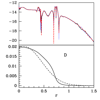
Figure 3.1: Convergence test for the fluid variable $D$. The top panel shows $\ln(3\tau^{8h}/4)\equiv D^{8h}-D^{4h}$ (black line), $\ln(3\tau^{4h})\equiv 4\left(D^{4h}-D^{2h}\right)$ (blue dots), $\ln(12\tau^{2h})\equiv 16\left(D^{2h}-D^{h}\right)$ (red dashes) which have been scaled such that they will look identical if our solutions are well-described by a Richardson expansion. The bottom panel shows $D(r,0)$ (black dashes) and $D(r,t)$, where $t$ is the time at which we performed the convergence test. The initial data consisted of a self-gravitating fluid specified by a Gaussian function for $\rho_{\circ}$ centered at $r=0.1$ with an initial, linear velocity profile. The initial grid used for the coarsest solution shown is defined by the parameters $\{N_{a},N_{b},N_{c},\Delta r_{a}\}=\{200,300,20,0.005\}$; please see Section 3.8 for definitions of these variables.

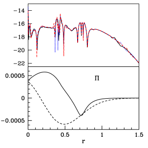
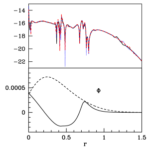
Figure 3.2: Convergence test for the fluid variable $\Pi$ (left) and $\Phi$ (right). The top panel of each figure show the scaled truncation error estimates for the respective fluid variable as described for the grid function $D$ in the caption to Figure 3.1. The bottom panels show $\Pi(r,0)$ and $\Phi(r,0)$ (dashed), and $\Pi(r,t)$ and $\Phi(r,t)$ (solid) where $t$ is the time at which convergence is tested.

To illustrate convergence properties of finite difference approximations, we show the convergence of results from our hydrodynamic code in Figures 3.1- 3.2. Even though finite volume methods (finite volume methods will be discussed in Section 3.2) are based upon the idea of approximating integral equations instead of differential equations, the above analysis still holds for finite volume solutions [52]. Shown in Figures 3.1- 3.2 are—respectively—$D$ (2.123), $\Pi$ (2.144), and $\Phi$ (2.145). The scaled truncation error estimates shown in the top panels of each figure demonstrate how the code exhibits the expected dependence on $h$ from Richardson’s expansion (3.10-3.11) for each dynamic fluid variable. The data taken from a time step before any discontinuities were observed in the solution to ensure that Richardson’s expansion would remain valid. In order to test the convergence of our regridding procedure—as described in Section 3.8.3—we calculated the truncation error estimates at a time after the grid was refined once.

3.2 Introduction to Conservative Methods

We employ High-Resolution Shock Capturing (HRSC) algorithms to solve the equations of motion for the fluid (2.146). Such methods have become increasingly popular in the field of relativistic hydrodynamics since they ensure: 1) conservation of the variables $\mathbf{q}$, and 2) discontinuities—e.g. shocks—are well resolved and travel at correct speeds. A key ingredient to these schemes is their use of solvers for the Riemann problem (see Section 3.3 for a discussion of the Riemann problem) at every cell interface. This is crucial for the conservative nature of these schemes since the solution to the Riemann problem is always a weak solution of the hyperbolic conservation laws. The “high-resolution” aspect of the algorithms denotes that in regions where the grid functions are smooth, the integration procedure is at least $O(\Delta r^{2})$ accurate. The HRSC methods used in this work have been used in several previous works such as [74], [66], and [64] to name only a few relevant papers. Also, many excellent references on conservative methods have been written by LeVeque [52, 53]; most of the development discussed here has been gleaned from these texts.

Conservation laws typically take the form of a differential equation, for example (2.101) or specifically (2.146). However, these “differential formulations” of the conservation laws do not directly follow from the original physical concepts involved and require that the dynamical variables be differentiable. Recall that our fluid fields are really thermodynamics quantities and, therefore, averages over finite fluid elements—which we will call cells in numerical contexts. Thus, the conservation laws result more naturally from integral equations.

In order to show the connection between the integral and differential formulations of conservation laws, let us consider the general case where ${x^{k}}$ is an $N$-dimensional orthogonal, spatial, coordinate system, and let $V_{i}$ and $S_{i}$ represent the volume and surface—respectively—of cell $\mathcal{C}_{i}$. A more covariant approach to conservative methods is given in [68]. So, in general, the differential form of the conservation law that we wish to consider is:

$$\partial_{t}\mathbf{q}\left(\vec{x},t\right)\ =\ -\nabla\cdot\vec{\mathbf{f}}\left(\mathbf{q}\right)\ +\ \mbox{\boldmath$\psi$}(\mathbf{q})$$ (3.20)

where $\vec{\mathbf{f}}$ is the flux density vector with components $\{\mathbf{f}^{k}\}$ in the basis of space-like coordinates $\{x^{k}\}$, and $\psi$ is a source term that involves no derivatives of the conserved variables $\mathbf{q}$. A variable in boldface represents a vector or set of quantities (as in equation (2.216)). Such a differential conservation law can be defined from the more general integral equation:

$$\frac{\partial}{\partial t}\int_{V_{i}}\mathbf{q}\left(\vec{x},t\right)dV\ =\ -\oint_{S_{i}}\vec{\mathbf{f}}\cdot d\vec{S}\ +\ \int_{V_{i}}\mbox{\boldmath$\psi$}\,dV$$ (3.21)

where—for example—we have assumed that the volume and surface that are being integrated over are that of the cell $\mathcal{C}_{i}$, but any arbitrary volume can be used in general. This equation implies that any change over time in the “amount” of $\mathbf{q}$ in volume $V_{i}$ is due to its flux at the surface of $V_{i}$, and from its source or sink within $V_{i}$. Integrating this equation with respect to time, we get:

$$\int_{V_{i}}\mathbf{q}\left(\vec{x},t_{2}\right)dV\,-\,\int_{V_{i}}\mathbf{q}\left(\vec{x},t_{1}\right)dV\ =\ -\int^{t_{2}}_{t_{1}}\oint_{S_{i}}\vec{\mathbf{f}}\cdot d\vec{S}\,dt\ +\ \int^{t_{2}}_{t_{1}}\int_{V_{i}}\mbox{\boldmath$\psi$}\,dVdt$$ (3.22)

The differential form (3.20) of the conservation law is derived from (3.22) by using Gauss’ Theorem:

$$\oint_{S_{i}}\vec{\mathbf{f}}\cdot d\vec{S}=\int_{V_{i}}\nabla\cdot\vec{\mathbf{f}}dV\quad.$$ (3.23)

Since Gauss’ theorem assumes that the functions are differentiable, the differential form only holds valid for systems that can be described by differentiable functions.

In order to arrive at a discretized form of (3.22), we must first define a few quantities. The average value of the conserved variable over the cell volume, $V_{i}$, is given by

$$\bar{\mathbf{q}}_{i}(t)\ =\ \frac{1}{V_{i}}\int_{V_{i}}\mathbf{q}\left(\vec{x},t\right)dV\quad.$$ (3.24)

If the cell $\mathcal{C}_{i}$ centered at $\vec{x}_{i}=(x^{1}_{i},\ldots,x^{N}_{i})$ has boundaries $[x^{1}_{i-1/2},\,x^{1}_{i+1/2}]\times\ldots\times[x^{N}_{i-1/2},\,x^{N}_{i+1/2}]$—where $x^{k}_{i}\equiv x_{\mathrm{min}}^{k}+(i-1)\Delta x^{k}$—then the flux integral in (3.21) and (3.22) can be written as:

$$\oint_{S_{i}}\vec{\mathbf{f}}\cdot d\vec{S}\ =\ \sum_{k=1}^{N}\left(\int_{S_{i+1/2}^{k}}\mathbf{f}^{k}\,dS\quad-\quad\int_{S_{i-1/2}^{k}}\mathbf{f}^{k}\,dS\right)\\$$ (3.25)

where the surface $S^{k}_{i+1/2}$—for instance—is defined as the isosurface of constant $x^{k}=x^{k}_{i+1/2}$. If we define a generalized numerical flux function to be the time average between two time steps of one of these integrals,

$$\mathbf{\mathcal{F}}^{k}_{i+1/2}\left(\mathbf{q}(x,t^{n})\right)=\frac{1}{\Delta t}\int^{t^{n+1}}_{t^{n}}\int_{S_{i+1/2}^{k}}\mathbf{f}^{k}\,dS\,dt\quad,$$ (3.26)

then we can rewrite (3.22)—with (3.25) and (3.24)—as

$$\bar{\mathbf{q}}_{i}(t^{n+1})\,-\,\bar{\mathbf{q}}_{i}(t^{n})\ =\ -\frac{\Delta t}{V_{i}}\sum_{k=1}^{N}\left(\mathbf{\mathcal{F}}^{k}_{i+1/2}-\mathbf{\mathcal{F}}^{k}_{i-1/2}\right)\ +\ \frac{1}{V_{i}}\int^{t^{n+1}}_{t^{n}}\int_{V_{i}}\mbox{\boldmath$\psi$}\,dVdt$$ (3.27)

3.2.1 Example: Spherical Symmetry

As a specific illustration, we will show how to go about deriving the spherically-symmetric version of the discretized conservation equation (3.27).

First, note that all functions are independent of $\phi$ and $\theta$. This means that the only non-zero flux component is the $r$-component, which we will denote $\mathbf{f}(q)$. Thus the numerical flux, $\mathbf{\mathcal{F}}_{i+1/2}$, becomes:

$$\mathbf{\mathcal{F}}_{i+1/2}\left(\mathbf{q}(r,t^{n})\right)\ = \ \frac{1}{\Delta t}\int^{t^{n+1}}_{t^{n}}\int_{S_{i+1/2}}\mathbf{f}\,dS\,dt$$ (3.28)

$$= \ 4\,\pi\,r^{2}_{i+1/2}\,\mathbf{F}_{i+1/2}$$ (3.29)

where $\mathbf{F}_{i+1/2}$ is the numerical flux defined by

$$\mathbf{F}^{n}_{i}=\frac{1}{\Delta t}\int^{t^{n+1}}_{t^{n}}\mathbf{f}(\mathbf{q}(x_{i},t))\ dt\quad.$$ (3.30)

With

$$V_{i}\ =\ \frac{4\pi}{3}\left(r^{3}_{i+1/2}-r^{3}_{i-1/2}\right)$$ (3.31)

the discretized equations for a finite volume are:

$$\mathbf{\bar{q}}^{n+1}_{i}\ =\ \mathbf{\bar{q}}^{n}_{i}\,-\,\frac{3\,\Delta t}{r^{3}_{i+1/2}-r^{3}_{i-1/2}}\left[\left(r^{2}X\mathbf{F}\right)^{n}_{i+1/2}-\left(r^{2}X\mathbf{F}\right)^{n}_{i-1/2}\right]\,+\,\Delta t\,\mbox{\boldmath$\bar{\psi}$}_{i}$$ (3.32)

where

$$\mbox{\boldmath$\bar{\psi}$}_{i}\ \equiv\ \frac{1}{\Delta t\left(r^{3}_{i+1/2}-r^{3}_{i-1/2}\right)}\ \int^{r_{i+1/2}}_{r_{i-1/2}}\int^{t^{n+1}}_{t^{n}}\mbox{\boldmath$\psi$}\,r^{2}\,dr\,dt\quad.$$ (3.33)

In practice, the average of the source, $\mbox{\boldmath$\bar{\psi}$}_{i}$, is approximated by the “source of the average”, $\mbox{\boldmath$\psi$}(\mathbf{\bar{q}}_{i})$.

The above equation (3.32) provides the basic form of the discretized equation that we solve. However, to complete the solution, we need a good way of determining the numerical flux, $\mathbf{F}_{i+1/2}$. Computing a good numerical flux constitutes the real art of implementing conservative methods.

3.3 The Riemann Problem and Godunov-type Methods

A Riemann problem seeks a solution to the equation

$$\partial_{t}q+\partial_{x}f=0$$ (3.34)

given piecewise constant initial data about an interface at $x=0$:

$$q(x,0)=\left\{\begin{array}[]{ll}q^{L}&x<0\\ q^{R}&x>0\end{array}\right.\quad.$$ (3.35)

A realization of this one-dimensional problem can be represented as a tube with two states of fluid that are separated by a removable partition. For example, the two states can have different pressures and/or densities. If the gas in either side has a non-zero velocity initially, then the problem falls under the more general class of shock tube problems. At $t=0$, the interface is removed and the two fluid components are allowed to mix. Shock tubes have been studied for years in the laboratory to understand how shock waves develop and propagate, and a schematic illustration of a shock tube is given in Figure 3.3.

Figure 3.3: A shock tube representing a Riemann problem. The tube is filled with fluid in two different states, separated by a removable interface.

The solution to the one-dimensional (scalar) Riemann problem obviously depends on the nature of the flux function $f$, since that function provides information regarding the characteristics of the equation. The Riemann problem has been studied extensively for many different flux functions, and much has been deduced from these investigations. For example, it is easy to show that a shock wave will develop and move toward $x=\infty$ if $q^{L}>q^{R}$ and $f(q^{L}),f(q^{R})>0$. Using, the Rankine-Hugoniot jump condition

$$\mathbf{f}(\mathbf{q}^{R})-\mathbf{f}(\mathbf{q}^{L})=s\left(\mathbf{q}^{R}-\mathbf{q}^{L}\right)$$ (3.36)

we can find the shock speed, $s$. The solution to the Riemann problem is then

$$q(x,t)=\left\{\begin{array}[]{ll}q^{L}&x<st\\ q^{R}&x>st\end{array}\right.\quad.$$ (3.37)

If instead we have $q^{L}<q^{R}$, $\{f(q^{L}),f(q^{R})\}>0$, and $f^{\prime\prime}(q)>0$, then the resulting evolution will describe a rarefaction fan, which is a self-similar solution [52]:

$$q(x,t)=\left\{\begin{array}[]{ll}q^{L}&x<f^{\prime}(q^{L})t\\[5.69046pt] Z(x/t)&f^{\prime}(q^{L})t<x<f^{\prime}(q^{R})t\\[5.69046pt] q^{R}&x>f^{\prime}(q^{R})t\end{array}\right.\quad.$$ (3.38)

where $Z(\mathcal{X})$ is the solution to the characteristic equation $f^{\prime}(Z(\mathcal{X}))=\mathcal{X}$.

However, when the conservation equation consists of many, coupled equations, much of the knowledge gleaned from the one-dimensional case cannot be directly used. However, it is still instructive to study the one-dimensional case, and many successful vector Riemann solvers have been based on features of the scalar problem. Since a vector problem can be approximated—to some extent—as a linear combination of scalar problems, we expect to find both shocks and rarefaction waves coming from a single interface. In fact, the vector Euler equations—(3.34) where $q$ and $f$ are now vectors—yields three primary wave solutions: shock, rarefaction and contact discontinuity. Let us take $\mathbf{w}=\left[P,v,\rho_{\circ}\right]^{T}$ to be the vector of primitive variables, and let us setup a vector Riemann problem with two states, $\mathbf{q}^{L}=\mathbf{q}(\mathbf{w}^{L})$ and $\mathbf{q}^{R}=\mathbf{q}(\mathbf{w}^{R})$. Then an example of a possible solution to this Riemann is given in Figure 3.4, where we have assumed that the left state is the one of greater pressure and density. The solution can be described by four basic states:

$$\mathbf{w}^{L}=\left[\begin{array}[]{c}P^{L}\\ v^{L}\\ \rho_{\circ}^{L}\end{array}\right]\ ,\ \mathbf{w}^{L*}=\left[\begin{array}[]{c}P^{*}\\ v^{*}\\ \rho_{\circ}^{L*}\end{array}\right]\ ,\ \mathbf{w}^{R*}=\left[\begin{array}[]{c}P^{*}\\ v^{*}\\ \rho_{\circ}^{R*}\end{array}\right]\ ,\ \mathbf{w}^{R}=\left[\begin{array}[]{c}P^{R}\\ v^{R}\\ \rho_{\circ}^{R}\end{array}\right]\ ,\$$ (3.39)

The rarefaction, as usual, travels into the high-density region and represents a continuum of states between $\mathbf{w}^{L}$ and $\mathbf{w}^{L*}$. The two intermediate states, $\mathbf{w}^{L*}$ and $\mathbf{w}^{R*}$, are separated by the contact discontinuity that travels with velocity $v^{*}$ and is discontinuous only in the density, $\rho_{\circ}$. The shock represents a discontinuity in all three fields and has the reverse role of the rarefaction—it travels into the less dense region and increases the pressure in its wake.

Figure 3.4: A graphical representation of a generic solution to the vector Riemann problem for the Euler equations. The world lines of the waves are shown as straight lines that separate unique states of the fluid. Hence, the effect the different waves have on the fluid is clearly seen. The values of the primitive variables in these distinct states are also shown. The rarefaction represents a continuum of states that is represented here by a fan-like ensemble of world lines.

Considering the discretized equation (3.32) derived in the previous section, we see that it describes a solution for averages of $\mathbf{q}$ over cell volumes. The cell averages, $\mathbf{\bar{q}}_{i}$ and $\mathbf{\bar{q}}_{i+1}$, can be viewed as representing piecewise constant initial data about the interface at $r=r_{i+1/2}$. Since $\mathbf{\bar{q}}_{i}\neq\mathbf{\bar{q}}_{i+1}$ in general, then we can think of the update procedure along this cell border as a Riemann problem. Such methods that describe the numerical solution in this way and utilize the Riemann solution at each cell border are called Godunov methods [52]. Specifically, a Godunov method is one in which the data are assumed to be piecewise-constant, but other methods extend the basic idea by employing higher-order interpolation schemes that assume that the data to be piecewise-linear, piecewise-parabolic, etc. Such higher-order schemes are thus called Godunov-type methods. In Section 3.4, we will describe the interpolation routines we used to make our solutions $2^{\mathrm{nd}}$-order away from shocks. We will also discuss how the Riemann solution is used to create a numerical flux function, $\mathcal{F}_{j}^{n}$, in the next two sub-sections. The two specific methods used are called Roe’s approximate solver, and the Marquina flux formula. These two methods use approximate solutions to the Riemann problem since finding the exact solution is often inefficient and not always necessary.

3.3.1 Roe’s Approximate Solver

We use a variant of Roe’s approximate Riemann solver [72], which is a Godunov-type method outlined in [52]. It is an approximate Riemann solver since it uses the exact Riemann solution to the approximate Riemann problem:

$$\partial_{t}\,\mathbf{q}\,+\,\frac{1}{r^{2}}\mathbf{A}\cdot\partial_{r}\left(r^{2}\mathbf{q}\right)\,=\,\mbox{\boldmath$\psi$}\quad.$$ (3.40)

where $\mathbf{A}$ represents a constant matrix at each step in the Riemann solution. The approximation then lies in that conservation equation has been linearized. However, this serves as a fair approximation if we choose $\mathbf{A}$ appropriately. Since we use Roe’s method to solve the Riemann problem at a cell border, the matrix $\mathbf{A}$ should only be dependent on the two states: $\mathbf{A}=\mathbf{A}(\mathbf{q}^{L},\mathbf{q}^{R})$. Determining this dependence lies at the heart of the method. A strict Roe method satisfies the following conditions:

1. $\mathbf{A}=\mathbf{A}(\mathbf{q}^{L},\mathbf{q}^{R})\rightarrow\mathbf{f}^{\prime}(\mathbf{\bar{q}})$ as $\mathbf{q}^{L},\mathbf{q}^{R}\rightarrow\mathbf{q}$

2. $\mathbf{A}(\mathbf{q}^{L},\mathbf{q}^{R})\left[\mathbf{q}^{L}-\mathbf{q}^{R}\right]=\mathbf{f}(\mathbf{q}^{L})-\mathbf{f}(\mathbf{q}^{L})$

3. $\mathbf{A}(\mathbf{q}^{L},\mathbf{q}^{R})$ has real eigenvalues and is non-singular.

The first condition guarantees that the linear problem will tend to the nonlinear one in smooth regions. The second criterion ensures that shock speeds are correctly calculated, as the Rankine-Hugoniot condition (3.36) dictates. The tie between these two equations can be seen by diagonalizing the linear system in criterion 2 and realizing that the eigenvalues—the diagonal elements—are the velocities of the shocks or contact discontinuities. Finally, the third criterion ensures that the system is hyperbolic.

Since a matrix meeting all this criteria is not known for the relativistic, spherically-symmetric case, we use a further approximation to Roe’s approximate Riemann solver. Specifically, we choose (following Romero et al. [74])

$$\mathbf{A}(\mathbf{q}^{L},\mathbf{q}^{R})=\left.\frac{\partial\mathbf{f}}{\partial\mathbf{q}}\right|_{\mathbf{q}=\hat{\mathbf{q}}}\quad,\quad\hat{\mathbf{q}}=\frac{1}{2}\left(\mathbf{q}^{L}+\mathbf{q}^{R}\right)\quad.$$ (3.41)

After solving the linear Riemann problem, the numerical flux of the solution can be taken to be [52]:

$$\mathbf{F}_{k+1/2}(t)=\frac{1}{2}\left[\mathbf{f}(\mathbf{q}^{L}_{k+1/2}(t))+\mathbf{f}(\mathbf{q}^{R}_{k+1/2}(t))-\sum_{m}\left|\lambda_{m}\right|\omega_{m}\mbox{\boldmath$\eta$}_{m}\right]\quad.$$ (3.42)

Here, $\lambda_{m}$ and $\mbox{\boldmath$\eta$}_{m}$ are the eigenvalues and right eigenvectors, respectively, of $\mathbf{A}$, $\mathbf{q}^{L}$ and $\mathbf{q}^{R}$ are, respectively, the values of $\mathbf{q}$ to the left and right of the cell boundary, and $\omega_{m}$ are the decomposed values of the jumps in the space of characteristic values:

$$\mathbf{q}^{R}-\mathbf{q}^{L}\ =\ \sum_{m}\omega_{m}\mbox{\boldmath$\eta$}_{m}\quad.$$ (3.43)

In order to calculate all quantities associated with $\mathbf{A}$, such as $\lambda_{m}$ and $\mbox{\boldmath$\eta$}_{m}$, we use the average of the left and right states, $\hat{\mathbf{q}}$ (3.41).

Figure 3.5: The Riemann solution using the approximate Roe method (dots), with initial data $\{P^{L},v^{L},\rho_{\circ}^{L}\}=\{100,0,1\}$, $\{P^{L},v^{L},\rho_{\circ}^{L}\}=\{1,0,1\}$ with $\Gamma=5/3$, using 200 cells. The $P$ and $\rho_{\circ}$ have been normalized to fit into the same plot. The solid line is the exact solution.

We note that this method is only an approximate Roe solver since it does not always satisfy Roe’s second criterion. Even though it does not guarantee the Rankine-Hugoniot condition in general, the method works well in practice. In Figure 3.5, we show a solution to a Riemann problem using this approximate Roe solver for each cell, where the Riemann problem was set up in the middle of the grid, i.e. at $x=0.5$. The solid line is the exact solution of the Riemann problem calculated by a routine given in [57]. The approximate solution compares favorably to the exact solution, especially in smooth regions where the Roe solution should be close to the exact solution. The numerical dissipation intrinsic to the method is observable near the shock and the edge of the rarefaction fan. In fact, the density is diffused to such a degree that it does not quite reach the exact solution’s value between the contact discontinuity and the shock.

As we will see in Section 3.11, the Roe solver leads to difficulties in certain situations. Since it is based on the solution to the linear Riemann problem, the solution—at the cell-scale—consists of only shocks and discontinuities. This leads to a problem when transonic rarefactions arise, i.e. when $f(q^{L})<0<f(q^{R})$.

3.3.2 Marquina’s Method

The Marquina Flux equation, as described in [29] and extensively tested in 2-D in [28], is an amalgamation of a Roe flux method and a Lax-Friedrichs method for a general system of conservation laws. The addition of the Lax-Friedrichs-like method acts as an entropy-fix to the Roe flux. Hence, Marquina’s equation—in many cases—seems to effectively add extra dissipation to the system. An example of this is shown in [28], where it was found that the use of an approximate Roe solver leads to the “carbuncle phenomenon” in front of the bow shock of a supersonic relativistic jet. The Marquina flux seems to eliminate the carbuncle and replicate the physics involved with the relativistic jet quite well. This suggests that it may be a useful technique in two—and even one—dimensions.

For  $m=1,\ldots,N$  do: If  $\left(\lambda_{m}(\tilde{\mathbf{q}}^{L})\ \lambda_{m}(\tilde{\mathbf{q}}^{R})\right)\,\geq\,0$ then If  $\lambda_{m}(\tilde{\mathbf{q}}^{L})>0$  then $\mbox{\boldmath$\phi$}^{+}_{m}\ =\ \mbox{\boldmath$\phi$}^{L}_{m}$ $\mbox{\boldmath$\phi$}^{-}_{m}\ =\ 0$ else $\mbox{\boldmath$\phi$}^{+}_{m}\ =\ 0$ $\mbox{\boldmath$\phi$}^{-}_{m}\ =\ \mbox{\boldmath$\phi$}^{R}_{m}$ end if else $\xi_{m}={\max}\left(\left|\lambda_{m}(\tilde{\mathbf{q}}^{L})\right|,\left|\lambda_{m}(\tilde{\mathbf{q}}^{R})\right|\right)$ $\mbox{\boldmath$\phi$}^{+}_{m}\ =\frac{1}{2}\left(\mbox{\boldmath$\phi$}^{L}_{m}\ +\ \xi_{m}\omega_{m}^{L}\right)$ $\mbox{\boldmath$\phi$}^{-}_{m}\ =\frac{1}{2}\left(\mbox{\boldmath$\phi$}^{R}_{m}\ -\ \xi_{m}\omega_{m}^{R}\right)$ end if $$\mathbf{F}(\tilde{\mathbf{q}}^{L},\tilde{\mathbf{q}}^{R})=\sum_{m=1}^{N}\left(\mbox{\boldmath$\phi$}^{+}_{m}\mbox{\boldmath$\eta$}_{m}(\tilde{\mathbf{q}}^{L})+\mbox{\boldmath$\phi$}^{-}_{m}\mbox{\boldmath$\eta$}_{m}(\tilde{\mathbf{q}}^{R})\right)$$

Table 3.1: The Marquina Flux Calculation.

The method utilizes the characteristic variables and fluxes, which are spectral expansions of the conservation variables and fluxes, in order to determine how Roe-like or Lax-Friedrichs-like the numerical flux will be. The characteristic variables, $\mbox{\boldmath$\omega$}_{m}$, and fluxes, $\mbox{\boldmath$\phi$}_{m}$, are defined as :

$$\begin{array}[]{l l}\mbox{\boldmath$\omega$}_{m}^{L}=\mathbf{l}_{m}(\mathbf{q}^{L})\cdot\mathbf{q}^{L}&\quad\mbox{\boldmath$\omega$}_{m}^{R}=\mathbf{l}_{m}(\mathbf{q}^{R})\cdot\mathbf{q}^{R}\\[14.22636pt] \mbox{\boldmath$\phi$}_{m}^{L}=\mathbf{l}_{m}(\mathbf{q}^{L})\cdot\mathbf{f}(\mathbf{q}^{L})&\quad\mbox{\boldmath$\phi$}_{m}^{R}=\mathbf{l}_{m}(\mathbf{q}^{R})\cdot\mathbf{f}(\mathbf{q}^{R})\end{array}$$ (3.44)

Here, $\mathbf{l}_{m}(\mathbf{q})$ and $\mbox{\boldmath$\eta$}_{m}(\mathbf{q})$ are the left and right eigenvectors, respectively, of $\mathbf{A}(\mathbf{q})$, the Jacobian matrix appearing in the conservation equation. Also, $m=1,\ldots,N$ enumerates the $N$ eigenvectors. The algorithm for calculating the Marquina flux is described in Table 3.1, where we recall that $\lambda_{m}(\mathbf{q})$ are the eigenvalues of $\mathbf{A}(\mathbf{q})$.

Figure 3.6: The Riemann solution using Marquina’s method (dots), with initial data $\{P^{L},v^{L},\rho_{\circ}^{L}\}=\{100,0,1\}$, $\{P^{L},v^{L},\rho_{\circ}^{L}\}=\{1,0,1\}$ with $\Gamma=5/3$, using 200 cells. The $P$ and $\rho_{\circ}$ have been normalized to fit into the same plot. The solid line is the exact solution.

Figure 3.6 shows a solution to the same Riemann problem considered in Figure 3.5 using the Marquina flux. For this particular Riemann problem, it seems that Roe’s method produces a slight Gibbs phenomenon near the origin of the rarefaction fan, while Marquina’s method results in the functions undershooting there. However, the two methods produce nearly identical results near the shock and contact discontinuity.

Even though we primarily use the approximate Roe solver, since it is computationally more efficient, the Marquina solver plays an important role in examining the instability near the sonic point in the self-similar solutions we obtain near Type II critical solutions. See Section 3.11 for further discussion of this point.

3.4 Reconstruction at the Cell Borders

Since the accuracy of the spatial differencing is constrained by the order of interpolation used to calculate the cell boundary values, a way to improve upon the $1^{\mathrm{st}}$-order accuracy of generic Godunov schemes is to increase the accuracy of the interpolation scheme. For example, Godunov methods are $1^{\mathrm{st}}$-order accurate since they assume that the data is piecewise-constant, but we can make the spatial differencing be $2\mathrm{nd}$-order or $3\mathrm{rd}$-order accurate by using piecewise-linear or piecewise-parabolic data, respectively. Even though piecewise-parabolic methods—such as PPM by Colella and Woodward [27]—have become more popular in recent years [31], we only use piecewise-linear methods here since they are straightforward to implement yet still provide well-resolved discontinuities.

Since shocks naturally arise in fluid dynamical evolutions, we require that the interpolation procedure capture shocks well so that spurious oscillations—in the form of Gibbs phenomena—do not occur. To minimize such numerical artifacts, we use linear, slope-limiting interpolators to calculate the border values $\mathbf{\bar{q}}^{L}$ and $\mathbf{\bar{q}}^{R}$. These are found by first interpolating for the primitive variables $\mathbf{\bar{w}}^{L}$, $\mathbf{\bar{w}}^{R}$ at the border, then setting $\mathbf{\bar{q}}^{L}=\mathbf{q}(\mathbf{\bar{w}}^{L})$ and $\mathbf{\bar{q}}^{R}=\mathbf{q}(\mathbf{\bar{w}}^{R})$ using the definitions of $\mathbf{q}(\mathbf{w})$ (2.123-2.126). We have found that by interpolating $\mathbf{\bar{w}}$ instead of $\mathbf{\bar{q}}$ the numerical procedure generally leads to smoother solutions and fewer instabilities. Specifically, the slope-limiting interpolation is carried out in the following fashion:

$$\mathbf{\bar{w}}^{L}_{k+1/2}\ =\ \mathbf{\bar{w}}_{k}+\mbox{\boldmath$\sigma$}_{k}\left(r_{k+1/2}-r_{k}\right)$$ (3.45)

$$\mathbf{\bar{w}}^{R}_{k+1/2}\ =\ \mathbf{\bar{w}}_{k}+\mbox{\boldmath$\sigma$}_{k+1}\left(r_{k+1/2}-r_{k+1}\right)$$ (3.46)

where the $\mbox{\boldmath$\sigma$}_{k}$ is the slope obtained from the slope-limiting function of given slopes

$$\mathbf{s}_{k+1/2}\equiv\left(\mathbf{\bar{w}}_{k+1}-\mathbf{\bar{w}}_{k}\right)/\left(r_{k+1}-r_{k}\right)$$ (3.47)

and $\mathbf{s}_{k-1/2}$. For instance, if we use the minmod slope-limiter defined by

$$\mathrm{minmod}(a,b)=\left\{\begin{array}[]{r@{\qquad}l}0&\mathrm{if}\quad ab<0\\ a&\mathrm{if}\quad|a|<|b|\quad\mathrm{and}\quad ab>0\\ b&\mathrm{if}\quad|b|<|a|\quad\mathrm{and}\quad ab>0\end{array}\right.$$ (3.48)

then

$$\mbox{\boldmath$\sigma$}_{k}=\mathrm{minmod}(\mathbf{s}_{k-1/2},\mathbf{s}_{k+1/2})\quad.$$ (3.49)

Determining what slopes to use at each border ultimately decides how shocks are resolved. In Figure 3.7, we plot $\mbox{\boldmath$\sigma$}_{k}$ computed using different schemes. The slopes represented by the black line are calculated by setting $\mbox{\boldmath$\sigma$}_{k}=0$, the blue dots from setting $\mbox{\boldmath$\sigma$}_{k}=\mathbf{s}_{k+1/2}$ always, and the red dashes are from $\mbox{\boldmath$\sigma$}_{k}=\mathrm{minmod}(\mathbf{s}_{k-1/2},\mathbf{s}_{k+1/2})$. Like most slope-limiters, the minmod function attempts to diffuse numerical oscillations—whose wavelengths are $2\Delta r$—by setting the slope to $0$ when adjacent slopes change sign. Also, it always uses the less steep slope, so that discontinuities are always well resolved with little overshooting or Gibbs phenomena. As can be seen in the figure, use of a non-limited slope obviously makes the solution overshoot the shock.

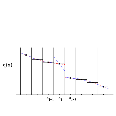
Figure 3.7: Results of different methods for calculating the slopes used in the linear interpolation procedure that estimates $\mathbf{\bar{q}}$ at cell borders. Here, the black horizontal lines represent piecewise-constant interpolation, the blues dots illustrate second order interpolation without limiting, and the red dashes represent second order interpolation with limiting.

We have tried other slope-limiters, such as the MC limiter and the Superbee limiter, but found the minmod limiter to provide the most stable calculations of near-threshold solutions (see [65] and references therein for descriptions of the MC and Superbee limiters). Since the MC and Superbee limiters resolve discontinuities more accurately, they lack minmod’s diffusiveness that seems to help dampen the instability observed near the sonic point of near-critical solutions (see Section 3.11 for a discussion of the instability mentioned here).

From the definition of $\mathrm{minmod}$, the limited slopes can be shown to be $0$ at extrema of $\mathbf{\bar{q}}$, such as near discontinuities and shocks. Thus, the interpolation procedure at the extrema reduces to a $1^{\mathrm{st}}$-order scheme, making the numerical solution there $1^{\mathrm{st}}$-order accurate. Fundamentally, with methods such as those used here, such behavior near shocks cannot be avoided since shocks in inviscid flow are not resolvable in the continuum limit. Thus, a piecewise-constant representation of the functions in a shock’s neighborhood is the best that can be done in any case, unless the position of shocks can be exactly traced. However, this makes convergence testing difficult since the solution’s convergence will be reduced from $2^{\mathrm{nd}}$-order to $1^{\mathrm{st}}$-order in regions where shocks—or any other extrema of $\mathbf{\bar{q}}$—propagate.

Non-oscillatory interpolation schemes have even been devised for arbitrary interpolation orders. For the regridding process described in Section 3.8.3, we use the so-called Essentially Non-Oscillatory (ENO) scheme originally developed by Shu [81]. The algorithm is especially powerful since it can be used to perform an interpolation of arbitrary order—only restricted by the number of available grid points from which to sample. The particular routine we use was written by Olabarrieta [67], and we have found that a $3^{\mathrm{rd}}$-order ENO interpolation is sufficient for our current work.

3.5 Time Integration Procedures

In order to make the entire differencing procedure $2^{\mathrm{nd}}$-order accurate, the differencing with respect to $t$ needs to also be adjusted since (3.32) is only differenced to $O(\Delta t)$. Explicit methods are usually used for performing the time integration in conservative schemes since conservative methods usually entail a myriad of other expensive steps. A simple way of making the method explicit is to split temporal and spatial difference operators using the method of lines, which entails integrating along each direction—-spatial and temporal—separately. Since all conservation equations take the form

$$\frac{d\mathbf{q}}{dt}=L(\mathbf{q})$$ (3.50)

we can solve this equation, after spatial discretization, as a system of ODEs. Here, $L$ includes the spatial differential operator as well as the source term. The discrete version, $\hat{L}$, can easily be inferred from the discretized EOM (3.32).

In predictor-corrector methods, intermediate values—$\mathbf{\bar{q}}^{n*}_{j}$ or $\mathbf{\bar{q}}^{n+1/2}_{j}$—are first calculated by the predictor step and then used in the corrector step to obtain the final updated values, $\mathbf{\bar{q}}^{n+1}_{j}$. For the modified Euler or Huen’s method, the following two equations define the predictor and corrector steps, respectively:

$$\bar{\mathbf{q}}^{*}_{j}=\bar{\mathbf{q}}^{n}_{j}+\Delta t\,\hat{L}(\bar{\mathbf{q}}^{n})$$ (3.51)

$$\bar{\mathbf{q}}^{n+1}_{j}=\frac{1}{2}\left[\bar{\mathbf{q}}^{n}_{j}+\bar{\mathbf{q}}^{*}_{j}+\Delta t\,\hat{L}(\bar{\mathbf{q}}^{*})\right]$$ (3.52)

The predicted values, $\mathbf{\bar{q}}^{*}_{j}$, can be interpreted as $1^{\mathrm{st}}$-order approximations to the corrected values, $\mathbf{\bar{q}}^{n+1}_{j}$.

Another commonly used method is the half-step predictor-corrector method, which is equivalent to a $2^{\mathrm{nd}}$-order Runge-Kutta technique. The half-step update does a $1^{\mathrm{st}}$-order predictor step integration to $t=t^{n+1/2}$, and then uses the slope at the half-step to evolve to $t=t^{n+1}$

$$\mathbf{q}^{n+1/2}=\mathbf{q}^{n}+\frac{\Delta t}{2}\hat{L}(\mathbf{q}^{n})$$ (3.53)

$$\mathbf{q}^{n+1}=\mathbf{q}^{n}+\Delta t\hat{L}(\mathbf{q}^{n+1/2})$$ (3.54)

We see little difference between the two methods in practice, even though Huen’s method has been shown to be the only $2^{\mathrm{nd}}$-order predictor-corrector method to be Total-Variation-Diminishing (TVD). TVD analysis is a way to demonstrate whether an algorithm is stable by seeing whether the quantity:

$$\mathrm{TV}\left(\mathbf{\bar{q}}^{n}\right)\equiv\sum_{j}\left|\mathbf{\bar{q}}^{n}_{j+1}-\mathbf{\bar{q}}^{n}_{j}\right|$$ (3.55)

monotonically decreases over time [52]. If it does, then the method is TVD. Hence, we use Huen’s method for all of the computations described here.

The stencil used for a generic predictor-corrector method (such as Huen’s method) is shown in Figure 3.8. The stencil is $5$ cells wide in our case because the slope-limiter uses this many points to determine the optimal process for reconstructing the values, $\mathbf{q}^{L}$ and $\mathbf{q}^{R}$, at each border.

Figure 3.8: Stencil depicting the update scheme for cell $\mathcal{C}_{j}$ from time step $n$ to time step $n+1$ using piecewise-linear reconstruction. The unfilled shapes represent the “predicted” grid function values, those calculated during the predictor step. The predicted state is labeled $n^{*}$ or $n+1/2$ depending on whether Huen’s method or the half-step method is used, respectively. The vertical bars represent cell boundaries.

The Courant-Friedrichs-Lewy (CFL) condition for these schemes essentially reduces to ensuring that the physical domain of dependence as determined by the largest characteristic speed $\lambda_{\max}$ is contained in the numerical domain of dependence:

$$\lambda_{\mathrm{CFL}}\ \equiv\ \frac{\Delta t}{\Delta r}<\frac{1}{\left|\lambda_{{\max}}\right|}$$ (3.56)

Throughout this work, we use $\lambda_{\mathrm{CFL}}=0.4$.

3.6 Primitive Variable Calculation

Since only the conservative variables are evolved by the HRSC schemes discussed above, the primitive variables must be derived from the conservative variables after each predictor or corrector step in order to compute fluxes $\mathbf{f}$ and source functions $\psi$ for the next evolution step. This involves inverting the three equations $\mathbf{q}=\mathbf{q}(\mathbf{w})$, which are given by the definitions of the conservative variables (2.123-2.126), for the three unknown primitive variables $\mathbf{w}$. We know of no closed-form expressions for the inverted equations, and so we must solve for $\mathbf{w}(\mathbf{q})$ numerically. At each grid point, we use a Newton-Raphson method to find the values of $\mathbf{w}$ that minimize the residuals of the conservative variable definitions (2.123-2.126). Instead of solving the full $3$-by-$3$ system at each point, an identity function $\mathcal{I}$—derived from (2.123-2.126)—is used as a residual, making the solution process one-dimensional. This makes the procedure much more efficient, especially since it needs to be executed $2N$ times per time step, where $N$ is the number of spatial grid points.

One obvious choice of the identity, which is commonly used [74, 65], is:

$$S-v\left(E+P\right)\ =\ 0\quad.$$ (3.57)

We divide by $v$ and express $S$ in terms of $D$ and $\mathbf{w}$ to get the final residual of

$$\mathcal{I}_{1}(P)\ =\ D\left[\frac{W(P)}{a}-1\right]+P\left[\,\mathcal{G}{W(P)}^{2}-1\,\right]-\tau$$ (3.58)

where (2.116) has been used to eliminate $\epsilon$, and $W(P)$ is given by (2.143):

$$W(P)=\sqrt{\frac{\left(\tau+D+P\right)^{2}}{\left(\tau+D+P\right)^{2}-S^{2}}}\quad.$$ (3.59)

In practice, this residual leads to inaccurate calculations of $\mathbf{w}$ for relativistic flows since the numerical evaluation of (3.59) as $|v|\rightarrow 1$ becomes less precise due to the fact that the numerator—$S$—and the denominator—$\left(\tau+D+P\right)$—both grow to infinity in that limit. In order to calculate $v$ more accurately in this limit, a different residual, which was first developed in [65], is used:

$$\mathcal{I}_{2}(H)\ =\ HW^{2}-\tau-D-P$$ (3.60)

where $H$ is the enthalpy,

$$H\ \equiv\ \rho_{\circ}h=\rho_{\circ}\left(1+\epsilon+P/\rho_{\circ}\right)\quad.$$ (3.61)

Using $H$ as the independent variable instead of $P$ allows us to calculate $v$ more precisely in relativistic flows and avoids the calculation of super-luminal velocities. Specifically, we compute:

$$v=v(\Lambda)=\frac{1}{2\Lambda}\left(\sqrt{1+4\Lambda^{2}}-1\right)$$ (3.62)

where $\Lambda\equiv S/H$. We note that equation (3.62) is simply an identity based on the definition of $W$ and the fact that $\Lambda=W^{2}v$.

The overall method used to find the primitive variables is outlined in Table 3.2. Depending on how relativistic or non-relativistic the flow is, different methods for calculating the residual $\mathcal{I}_{2}$ and its “Jacobian” $\mathcal{I}_{2}^{\prime}=\partial\mathcal{I}_{2}/\partial H$ are used in order to increase the accuracy of $\mathbf{w}$; these methods are described in Table 3.3. The “non-relativistic” and “intermediate” methods originated from Neilsen [65], where flows in the ultra-relativistic limit were also studied. However, we have found that, in the ultra-relativistic limit where $\Lambda\rightarrow\infty$, the intermediate method still gives imprecise results that are essentially due to the diminishing precision of calculating the deviation

$$1-v\left(\Lambda\right)=1-\sqrt{1+1/4\Lambda^{2}}+1/2\left|\Lambda\right|\quad.$$ (3.63)

Even though the above methods improved the accuracy of the primitive variable calculation, significant errors still remain for highly-relativistic flows ($W>10^{5}$) with $P$ and $\rho_{\circ}$ being different by orders of magnitude—.e.g. when $P\gg\rho_{\circ}$ or $\rho_{\circ}\gg P$. In these regimes, machine precision limits the accuracy of the calculation since terms in $\mathcal{I}_{2}$ and $\mathcal{I}_{2}^{\prime}$ become numerically insignificant even though their presence is essential to finding the solution.

$\underline{\mathrm{Given}\ \left\{D,S,\tau,a\right\}^{\mathrm{new}}\ \mathrm{at}\ t=t^{\mathrm{new}}\ \mathrm{and}\ \left\{\rho_{\circ},P\right\}^{\mathrm{old}}\ \mathrm{at}\ t=t^{\mathrm{old}}}$ : $\displaystyle\mathbf{\#1)}$ $\displaystyle\mathcal{G}\equiv\frac{\Gamma}{\Gamma-1}\quad,\quad H^{\mathrm{new}}=\rho_{\circ}^{\mathrm{old}}+\mathcal{G}P^{\mathrm{old}}$ $\displaystyle\underline{\hskip 72.26999pt}$ $\displaystyle\mathbf{\#3)}$ $\displaystyle H=H^{\mathrm{new}}\quad,\quad\Lambda=S\,/\,H$ $\displaystyle\mathbf{\#4)}$ $\displaystyle\mathrm{Calculate}\ \left\{\mathcal{I}_{2}\,,\,\mathcal{I}_{2}^{\,\prime}\,,P,v,\rho_{\circ}\right\}$ $\displaystyle\mathbf{\#5)}$ $\displaystyle\Delta H=-\,\mathcal{I}_{2}\,/\,\mathcal{I}_{2}^{\,\prime}\quad,\quad H^{\mathrm{new}}=H+\Delta H$ $\displaystyle\mathbf{\#6)}$ $\displaystyle\mbox{Repeat Steps {\#3 -- \#5} \ until }\ \left(\,|\Delta H/H|<\mathtt{tol}\,\right)$ $\displaystyle\underline{\hskip 72.26999pt}$ $\displaystyle\mathbf{\#7)}$ $\displaystyle P^{\mathrm{new}}\,=\,P\quad,\quad v^{\mathrm{new}}\,=\,v\quad,\quad\rho_{\circ}^{\mathrm{new}}\,=\,\rho_{\circ}$

Table 3.2: The Point-wise Newton-Raphson method used to construct the primitive variables from the conservative variables and geometry. The calculation is performed after the conservative variables have been integrated to a new time step at $t=t^{\mathrm{new}}$, and $a$ has been found via the Hamiltonian constraint. A few variables—$P$ and $\rho_{\circ}$—are needed from the previous time step, $t^{\mathrm{old}}$, as guesses for the iteration process. Here, $\mathcal{I}_{2}$—given by (3.60)—is the residual that is numerically minimized.

If $\left(|\Lambda|>\Lambda_{\mathrm{High}}\right)\ \mathbf{\mathtt{then}}$ $b=\mbox{\Large$\frac{1}{2\left|\Lambda\right|}$}\quad,\quad B\equiv b^{2}\quad,\quad X(b)\equiv 1/W^{2}=2\sqrt{B}\left(\sqrt{B+1}-\sqrt{B}\right)$ $\rho_{\circ}=\mathtt{TAYLOR}_{8}\left[\mbox{\Large$\frac{D}{a}$}\sqrt{X(b)}\right]\quad,\quad P=\mathtt{TAYLOR}_{8}\left[\mbox{\Large$\frac{1}{\mathcal{G}}$}\left(H-\mbox{\Large$\frac{D}{a}$}\sqrt{X(b)}\right)\right]$ $v=\mathtt{sign}(S)\ \mathtt{TAYLOR}_{8}\left[\left(\sqrt{B+1}-\sqrt{B}\right)\right]$ $\mathcal{I}_{2}=\mathtt{TAYLOR}_{8}\left[H\mbox{\Large$\left(\frac{1}{X(b)}-\frac{1}{\mathcal{G}}\right)$}-\tau+D\left(\mbox{\Large$\frac{\sqrt{X(b)}}{a\mathcal{G}}$}-1\right)\right]$ $\mathcal{I}_{2}^{\prime}=\mathtt{TAYLOR}_{8}\left[\mbox{\Large$\frac{1}{2\sqrt{B+1}\left(\sqrt{B+1}-\sqrt{B}\right)}-\frac{1}{\mathcal{G}}+\left(\frac{D}{aH\mathcal{G}}\right)\frac{B^{1/4}\left(\sqrt{B+1}-\sqrt{B}\right)^{3/2}}{\sqrt{2}\sqrt{B+1}}$}\right]$ $\mathbf{\mathtt{Else}}$ $\mathbf{\mathtt{If}}\left(|\Lambda|>\Lambda_{\mathrm{Low}}\right)\ \mathbf{\mathtt{then}}$ $\quad\mathcal{Y}\ =\ \sqrt{1+4\Lambda^{2}}\quad,\quad v\ =\ \mbox{\Large$\frac{1}{2\Lambda}$}\left(\mathcal{Y}-1\right)\quad,\quad\mbox{\Large$\frac{\partial v}{\partial H}\ =\ -\frac{S}{H^{2}}\left[\frac{2}{\mathcal{Y}}-\frac{\left(\mathcal{Y}-1\right)}{2\Lambda^{2}}\right]$}$ $\mathbf{\mathtt{Else}}$ $\quad v\ =\ \left(1+\left(-1+\left(2+\left(-5+\left(14-42\,{\Lambda}^{2}\right){\Lambda}^{2}\right){\Lambda}^{2}\right){\Lambda}^{2}\right){\Lambda}^{2}\right)\Lambda$ $\quad\mbox{\Large$\frac{\partial v}{\partial H}\ =\ -\frac{S}{H^{2}}$}\ \left[1+\left(-3+\left(10+\left(-35+\left(126-462\,{\Lambda}^{2}\right){\Lambda}^{2}\right){\Lambda}^{2}\right){\Lambda}^{2}\right){\Lambda}^{2}\right]$ $\mathbf{\mathtt{End}}\,\mathbf{\mathtt{If}}$ $W=1\,/\sqrt{1-v^{2}}\quad,\quad P=\mbox{\Large$\frac{1}{\mathcal{G}}$}\left(H-\mbox{\Large$\frac{D}{aW}$}\right)\quad,\quad f(H)=HW^{2}\,-\tau-D-P$ $f^{\,\prime}(H)\ =\ W^{2}\left(1\,+\,2HW^{2}\,v\,\mbox{\Large$\frac{\partial v}{\partial H}$}\right)\,-\,\mbox{\Large$\frac{1}{\mathcal{G}}\left(1\,+\,\frac{DWv}{a}\,\frac{\partial v}{\partial H}\right)$}\quad,\quad\rho_{\circ}=\mbox{\Large$\frac{D}{aW}$}$ $\mathbf{\mathtt{End}}\,\mathbf{\mathtt{If}}$

Table 3.3: Pseudo-code for the calculation of $\left\{\mathcal{I}_{2},\mathcal{I}_{2}^{\,\prime},P,v,\rho_{\circ}\right\}$ used in the primitive variable construction procedure described in Table 3.2. See the next page for this figure’s caption.

(Caption for Table 3.3) Pseudo-code for the calculation of $\left\{\mathcal{I}_{2},\mathcal{I}_{2}^{\,\prime},P,v,\rho_{\circ}\right\}$ used in the primitive variable construction procedure described in Table 3.2. The procedure performs the calculation in three different ways depending in which regime the system resides. In the ultra-relativistic regime, $\left|\Lambda\right|$ becomes quite large and, subsequently, expanding the nonlinear expressions in powers of $b=1/2\left|\Lambda\right|$ becomes numerically more accurate. In the above table, $\mathtt{TAYLOR}_{8}$ represents the operation of taking the series expansion of its argument to $O(b^{8})$. Also, for the case when the system is non-relativistic—e.g. when $\left|\Lambda\right|\ll 1$—we use expansions up to $O(\Lambda^{9})$. In practice, the ultra-relativistic regime is defined by an adjustable parameter $\Lambda_{\mathrm{High}}$ and the non-relativistic regime by $\Lambda_{\mathrm{Low}}$. For example, in all the results shown here we used $\Lambda_{\mathrm{High}}=10^{2}$ and $\Lambda_{\mathrm{Low}}=10^{-4}$; these values ensure that the leading-order error terms in the ultra-relativistic and non-relativistic expansions are below the round-off error of the machines used.

3.7 The Floor

Contrary to evolutions in Lagrangian coordinates, flows computed using Eulerian coordinates often give rise to evacuated regions where the pressure and/or density vanish and near-luminal fluid velocities develop. Due to the finite precision of the calculations and the nature of the numerical methods employed, the evacuation often “overshoots” the vacuum state generating negative pressures or densities, which in turn leads to a plethora of unphysical, numerical consequences such as a complex $c_{s}$ or super-luminal velocities. This is one of the more troublesome problems encountered in numerical relativistic hydrodynamics and a completely satisfactory resolution is unfortunately still outstanding. In order to alleviate the evacuation problem and to avoid such catastrophic consequences, we require the dynamic fluid quantities—the conservative variables $\mathbf{q}$ (2.147)—to have values greater than or equal to a so-called “floor” state. In order to determine the floor state, we require $P,\rho_{\circ}>0$ and $|v|<1$ which implies that

$$D\ ,\ \left(\tau\pm\left|S\right|\right)\ >\ 0$$ (3.64)

Using the transformed (“new”) variables $\Pi,\Phi$, we implement this requirement in the following way

$$D\ = \ {\max}\left(D,\delta\right)$$ (3.65)

$$\Pi\ = \ {\max}\left(\Pi+D,2\delta\right)-D$$ (3.66)

$$\Phi\ = \ {\max}\left(\Phi+D,2\delta\right)-D$$ (3.67)

Notice that the $\Pi$ and $\Phi$ need not remain positive since $\tau\leq 0$ is physical as long as $E>0$. Since the floor state involves very little mass-energy, its use does not significantly affect the overall dynamics of the star. For example, Figure 5.7 shows how the scaling of the global maximum of ${T^{a}}_{a}$ as a function of $\ln\left(p^{\star}-p\right)$ is independent of the floor values. The most striking indication of the relative insignificance of the floor is the fact that the computed values for the critical velocity amplitude $p^{\star}$ are surprisingly in agreement, to within $4\times 10^{-5}$.

3.8 Description of the Numerical Grid and Refinement Procedures

In this section we describe the basic structure of the numerical domain used in the code. We start by describing the most basic grid—a uniform grid—to introduce the cell-centered grids used for finite volume methods. Then we describe the more complicated nonuniform and adaptive grid structure used to study self-similar collapse.

3.8.1 Ghost Cells and Uniform Grids

The entire numerical grid domain, $\Omega$, consists of two sub-domains: the physical domain, $\Omega_{o}$, and the ghost domain, $\Omega_{g}$. The physical domain represents the physical space that we are modeling, whereas the ghost domain is used to “extend” the grid so that the same update algorithm can be used on the entire physical domain (even for boundary points). For example, we require two ghost cells at each boundary because, as shown in Figure 3.8, the update method uses a 5-cell stencil. In this thesis, we define $N_{g}$ to be the number of ghost cells at each boundary (so that if $\Omega_{o}$ has two boundaries, and $N_{g}=2$, then a total of $4$ ghost cells are used).

In the following, we describe how ghost cells are defined in spherical symmetry.

Let $\mathcal{C}_{i}$ denote the $i^{th}$ cell that is centered about $r=r_{i}$, with $i=1,\ldots,N_{r}$ and where $N_{r}$ is the number of cells in $\Omega$. The domains are defined as:

$$\Omega_{g}=\left(\mathcal{C}_{1},\ldots,\mathcal{C}_{N_{g}},\mathcal{C}_{N_{r}-N_{g}+1},\ldots,\mathcal{C}_{N_{r}}\right)$$ (3.68)

$$\Omega_{o}=\left(\mathcal{C}_{N_{g}+1},\ldots,\mathcal{C}_{N_{r}-N_{g}}\right)$$ (3.69)

so that the two domains do not overlap:

$$\Omega_{o}\cap\Omega_{g}=\emptyset$$ (3.70)

This way, all the physical cells in $\Omega_{o}$ are updated using the same stencil; however, ghost cells near the origin are updated differently than those at the outer boundary (see the following sections).

The coordinate vector, $r_{i}$, that we use is defined as

$$r_{i}\equiv r_{\min}+\left(i-N_{g}-1/2\right)\Delta r\quad,\ i=1,\ldots,N_{r}\quad,$$ (3.71)

where

$$\Delta r\equiv\frac{r_{\max}-r_{\min}}{N_{r}-2N_{g}}$$ (3.72)

and where $r_{min}$ is the coordinate of the first physical cell’s left border and $r_{\max}$ is the coordinate of the last physical cell’s right border. That is, the first physical cell $\mathcal{C}_{N_{g}+1}$ is located at $r_{N_{g}+1}=r_{min}+\Delta r/2$, while the last physical cell $\mathcal{C}_{N_{r}-N_{g}}$ is located at $r_{N_{r}-N_{g}}=r_{\max}-\Delta r/2$ .

In spherical symmetry, one would typically set $r_{min}=0$. From the definition of the grid coordinates (3.71), it can easily be seen that the first physical cell is offset by $\Delta r/2$ from the origin; this way of discretizing the grid ensures that meshes can be refined in a consistent manner. We will denote discretized grid functions such that $Q_{i}^{n}$ denotes the value $Q(r_{i},t^{n})$. Figure 3.9 depicts how the domains are discretized.

Figure 3.9: Illustration of the spatial discretization of the solution domain. This example shows a sample discretization with $N_{r}=8$ and $N_{g}=2$. Squares denote the centers of cells, and the short vertical lines denote cell boundaries. The dashed vertical lines located at $r=r_{\min}$ and $r=r_{\max}$ separate the ghost cell domain, $\Omega_{g}$, from the physical domain, $\Omega_{o}$. The filled squares represent ghost cells, while the empty squares represent physical cells.

3.8.2 The Nonuniform Mesh

In order to track the CSS behavior of near critical solutions, we need to numerically resolve the dynamics that take place on continuously-decreasing spatio-temporal scales. From previous work in critical phenomena with perfect fluids, we know the qualitative behavior of the collapse and so we can tailor our refinement procedure accordingly. If this were not the case, we would have to resort to more sophisticated and general Adaptive Mesh Refinement (AMR) techniques such as Berger and Colella’s algorithm [6] for conservative systems. Since the self-similar regime focuses onto the origin at some finite proper time, the grid refinement is only needed near the origin. By using a nonuniform grid that is spaced logarithmically, we are able to concentrate computational resources on the most important region. Also, the logarithmic grid allows us to extend the outer boundary further than we would be able to with the same number of uniformly-spaced points, which subsequently reduces the effect the boundary conditions have on the interior solution.

The prescription for defining the initial grid and the refinement process was inspired by an algorithm used in [65]. However, we believe that there are a few details omitted, or not implemented in that work, that improve the method without any additional complexity, and so we provide them here.

As in [65], the portion of the grid not containing ghost zones consists of $3$ subdomains:

$$\begin{array}[]{l@{\ : \ }lll}\Omega_{a}&0\leq r\leq r_{a},&N_{a}\ \mathrm{cells},&\Delta r=\Delta r_{a};\\ \Omega_{b}&r_{a}<r<r_{b},&N_{b}\ \mathrm{cells},&\mathcal{R}_{i}\equiv\ln(r_{i}),\ \Delta\mathcal{R}=\mathcal{R}_{i+1/2}-\mathcal{R}_{i-1/2};\\ \Omega_{c}&r_{b}\leq r\leq r_{c},&N_{c}\ \mathrm{cells},&\Delta r=\Delta r_{c}.\\ \end{array}$$ (3.73)

where $\Delta r_{a}$, $\Delta\mathcal{R}$, and $\Delta r_{c}$ are all constant. The cell centers are always defined as the points that lie midway between two consecutive cell boundaries, so $\mathcal{C}_{i}$ is located at $r=r_{i}$ with boundaries at $r_{i-1/2}$ and $r_{i+1/2}$. This motivates the definition of $\Delta\mathcal{R}$ in (3.73).

The logarithmically-spaced grid segment, $\Omega_{b}$, smoothly (in $\Delta\mathcal{R}$) connects the higher resolution $\Omega_{a}$ grid adjoining the origin, to the lower resolution $\Omega_{c}$ grid abutting the outer boundary. In order for the different subdomains to connect smoothly, we demand that the grid-defining parameters satisfy the following relations:

$$e^{\mathcal{R}_{a}+\Delta\mathcal{R}}\,-\,e^{\mathcal{R}_{a}}\ =\ \Delta r_{a}\\$$ (3.74)

$$e^{\mathcal{R}_{b}}\,-\,e^{\mathcal{R}_{b}-\Delta\mathcal{R}}\ =\ \Delta r_{c}$$ (3.75)

In addition, we have three more equations that relate the lengths of the discrete subdomains to their resolutions:

$$r_{a}=N_{a}\Delta r_{a}\quad,\quad\mathcal{R}_{b}=N_{b}\Delta\mathcal{R}+\mathcal{R}_{a}\quad,\quad r_{c}=N_{c}\Delta r_{c}+r_{b}\quad.$$ (3.76)

Since we have five equations and 9 unknowns, $\{N_{a},\Delta r_{a},r_{a},N_{b},\Delta R,r_{b},N_{c},\Delta r_{c},r_{c}\}$, we need only provide any four parameters to uniquely specify the grid. There are many ways of specifying such a grid, but we have found that one way in particular ensures that the subdomains match smoothly for any choice of parameter values. First, notice that some parameters are integers, $\{N_{a},N_{b},N_{c}\}$, and some are floating-point values, $\{\Delta r_{a},r_{a},\Delta R,r_{b},\Delta r_{c},r_{c}=r_{\max}\}$. Specifying the floating-point parameter values—in general—will lead to non-integer values of $\{N_{a},N_{b},N_{c}\}$ which, in turn, would lead to a numerical inconsistency in the matching conditions (3.74) - (3.75). Thus, it is best to specify the integer-valued parameters and derive the rest. Since there are only three integer-valued parameters, we must specify one floating-point parameter as well. Because we are most interested in the dynamics that takes place within and near domain $\Omega_{a}$, we have found it convenient to specify $\Delta r_{a}$. Hence, we specify $\{N_{a},N_{b},N_{c},\Delta r_{a}\}$ and obtain the remaining parameters as follows.

From (3.74), we obtain an equation for $\Delta\mathcal{R}$:

$$\Delta\mathcal{R}=\ln\left(\frac{N_{a}+1}{N_{a}}\right)$$ (3.77)

Using this with (3.75) and (3.76), it can easily be seen that

$$\Delta r_{c}\ =\ \Delta r_{a}\left(\frac{N_{a}+1}{N_{a}}\right)^{N_{b}-1}$$ (3.78)

Finally, using (3.76) and (3.78), we get the remaining two grid parameters

$$r_{b}\ =\ \Delta r_{c}\left(N_{a}+1\right)$$ (3.79)

$$r_{{\max}}\ =\ r_{b}+N_{c}\Delta r_{c}\ =\ \Delta r_{c}\left(N_{a}+N_{c}+1\right)\quad.$$ (3.80)

3.8.3 The Refinement Procedure

In order to properly resolve CSS solutions, it is necessary to periodically add cells near the origin since this is where the spatial and temporal scales of the solution become the smallest. This is done by reducing $\Delta r_{a}$ by some fraction, $f_{\mathrm{reg}}$, and adding cells to $\Omega_{b}$ so as to maintain smoothness in $\Delta r(r)$ across the two subdomain boundaries. It can then easily be derived that the following is the transformation law of grid parameters during a refinement process:

$$\Delta r_{a}\ \longmapsto\ \frac{\Delta r_{a}}{f_{\mathrm{reg}}}$$ (3.81)

$$N_{a} \longmapsto N_{a}$$ (3.82)

$$N_{b} \longmapsto N_{b}+\Delta N_{b}$$ (3.83)

$$N_{c} \longmapsto N_{c}$$ (3.84)

where

$$\Delta N_{b}\ \equiv\ \mathrm{NINT}\left[\frac{\ln(f_{\mathrm{reg}})}{\Delta\mathcal{R}}\right]\quad,$$ (3.85)

And the NINT() function returns the nearest integer to its argument. Since the user-specified $f_{\mathrm{reg}}$ will not in general be such that $\Delta N_{b}$ is precisely integer-valued, we need to recalculate it from the $\mathrm{NINT}(\Delta N_{b})$. This is done by initially setting

$$\Delta N_{b} \ \equiv\ \mathrm{NINT}\left[\frac{\ln(f_{\mathrm{reg}}^{\prime})}{\Delta\mathcal{R}}\right]\quad$$ (3.86)

$$f_{\mathrm{reg}} = e^{\Delta N_{b}\ \Delta\mathcal{R}}\quad,$$ (3.87)

where $f_{\mathrm{reg}}^{\prime}$ is the user-specified value of $f_{\mathrm{reg}}$. After the refined coordinates are calculated, the grid functions are interpolated onto the new grid from the original grid via $3^{\mathrm{rd}}$-order ($4$-point) interpolation. Note, however, that the newly introduced coordinates exist only in $\Omega_{a}$ and for the first $\Delta N_{b}$ cells of $\Omega_{b}$. In particular, all cells in $\Omega_{c}$ and the original part of $\Omega_{b}$ remain at the same coordinate locations and consequently interpolation is not required there.

The decision as when to refine the grid is determined by tracking a feature of the solution and ensuring that there are a minimum number of cells between it and the origin. Since the solutions under study are CSS, this process is an easy one: in the self-similar regime, the solution looks functionally the same for all time, but on ever-decreasing scales. We have chosen to track the local maximum of $2m(r)/r$ that lies nearest to the origin, since it has empirically been found to always lie near the self-similarity horizon for near-critical solutions. Tracking ${\max}(2m(r)/r)$ also ensures that the approximate locations of any black hole surfaces that may arise will be resolved since ${\max}(2m(r)/r)\rightarrow 1$ as they form in our Schwarzschild-like coordinates. Hence, we refine the mesh when this maximum first passes within $r_{a}/f_{\mathrm{reg}}$, thereby requiring there to be between $N_{a}/f_{\mathrm{reg}}$ and $\sim\!N_{a}$ cells within the self-similar region.

In order to perform convergence tests of our nonuniform evolutions, we need a quantitative way for refining the mesh locally. Let

$$\{\Delta r_{a}(l),\Delta\mathcal{R}(l),\Delta r_{c}(l),N_{a}(l),N_{b}(l),N_{c}(l)\}$$

represent the grid parameters for a grid at level of refinement, $l$. The $l=0$ grid is called the base grid, from which the grid attributes of all other grids of $l\neq 0$ are calculated. The following is how we define the parameters of grids at higher levels of refinement:

$$\begin{array}[]{lll}N_{a}(l)=2^{l}N_{a}(0),&N_{b}(l)=2^{l}N_{b}(0),&N_{c}(l)=2^{l}N_{c}(0)\\[5.69046pt] \Delta r_{a}(l)=\Delta r_{a}(0)/2^{l},&\Delta\mathcal{R}(l)=\Delta\mathcal{R}(0)/2^{l},&\Delta r_{c}(l)=\Delta r_{c}(0)/2^{l}\end{array}\quad.$$ (3.88)

In all our runs, we have used $f_{\mathrm{reg}}^{\prime}=2$ so as to approximately double the resolution in $\Omega_{a}$ during each refinement. The other free grid parameters are usually chosen as functions of the given star data we start with. We pick an initial grid such that the $r_{a}$ is slightly larger than the stellar radius, $R_{\star}$, so that $r_{\max}$ is about $5-10R_{\star}$, and $N_{a}\simeq 300-600$. This places the outer boundary sufficiently far from the dynamical region while providing adequate initial resolution of the star. For example, the grid parameters used for the runs shown in Figure 3.10 for $l=0$, $\rho_{c}=0.05$ ($R_{\star}(\rho_{c}=0.05)\simeq 1.11$ in our unit-less coordinates, $K=1$) are $N_{a}=300$, $N_{b}(t=0)=500$, $N_{c}=20$, $\Delta r_{a}=0.005$ which leads to $r_{a}=1.5$ and $r_{\max}\simeq 8R_{\star}$.

Figure 3.10: The logarithm of the local resolution, $\Delta r(r)$, is plotted here as a function of radius. This particular run was for the nearest subcritical solution we were able to obtain for a star with $\rho_{c}=0.05$, $\Gamma=2$, and $K=1$; all but the second refinement is shown here. The free parameters that define the grid structure and refinement for this run are $N_{a}=300$, $N_{b}(t=0)=500$, $N_{c}=20$, $\Delta r_{a}=0.005$. These particular values are such that 208 cells are added to $\Omega_{b}$ at each refinement. The final value for $\Delta r_{a}$ is about $1.5\times 10^{-10}$.

3.9 The Numerical Solution of the Metric Functions

In this section, we describe the finite difference approximations we use to solve the Hamiltonian constraint (2.129) and the slicing condition (2.130). As examples, we use the form of the Hamiltonian constraint and slicing condition that they take when only the perfect fluid is present; it should be straightforward to extrapolate the discretization procedure for the geometric equations to the cases with different matter models.

Since we are using nonuniform grids, it is important to always use discretizations that are centered about the cell center. Also, we need to keep in mind that the metric functions are calculated at the cell borders as opposed to the cell centers, where the fluid quantities are calculated. Because of the particular form of the equations, it is best to difference $\ln(a_{j})$ and $\ln(\alpha_{j})$ instead of $a_{j}$ and $\alpha_{j}$ in order to increase the calculation’s precision. Thus, we difference the Hamiltonian constraint in the following way:

$$\ln(a_{j+1/2})-\ln(a_{j-1/2})=\left(r_{j+1/2}-r_{j-1/2}\right)\exp\left(\ln(a_{j+1/2})+\ln(a_{j-1/2})\right)$$

$$\quad\times\left[4\pi r_{j}\left(\tau_{j}+D_{j}\right)-\frac{1}{2r_{j}}\left(1-4\exp\left(-\ln(a_{j+1/2})-\ln(a_{j-1/2})\right)\right)\right]\quad\quad\quad,$$ (3.89)

and difference the slicing condition similarly:

$$\ln(\alpha_{j+1/2})-\ln(\alpha_{j-1/2})=\frac{1}{4}\left(r_{j+1/2}-r_{j-1/2}\right)\left(a_{j+1/2}+a_{j-1/2}\right)^{2}$$

$$\quad\quad\quad\times\left[4\pi r_{j}\left(S_{j}v_{j}+P_{j}\right)+\frac{1}{2r_{j}}\left(1-\frac{4}{\left(a_{j+1/2}+a_{j-1/2}\right)^{2}}\right)\right]\quad.$$ (3.90)

Since the slicing condition is a homogeneous ODE in $\alpha$, we start from $r=r_{\max}$ and solve the algebraic equation (3.90) for the unknown neighbor value, continuing the process to $r=r_{\min}$. However, integrating the Hamiltonian constraint is more difficult since it is inhomogeneous in $a$. A Newton-Raphson method is used to minimize the residual of (3.89) to solve for the unknown neighbor value, which is $a_{j+1/2}$, since we start the integration from $r=r_{\min}$.

In order to perform an independent residual test on our numerical solutions, we use the following distinct discretizations for the above metric equations. The independent residual for the Hamiltonian constraint is

$$\mathrm{Resid}^{\mathrm{HC}}_{j} = \frac{a_{j+3/2}+a_{j+1/2}-a_{j-1/2}-a_{j-3/2}}{2\left(r_{j+1}-r_{j-1}\right)}$$ (3.91)

$$- \frac{1}{4}\left(a_{j+1/2}+a_{j-1/2}\right)^{3}$$

$$\times \left[4\pi r_{j}\left(\tau_{j}+D_{j}\right)-\frac{1}{2r_{j}}\left(1-\frac{4}{\left(a_{j+1/2}+a_{j-1/2}\right)^{2}}\right)\right]\quad,$$ (3.92)

and the independent residual for the slicing condition is

$$\mathrm{Resid}^{\mathrm{SC}}_{j} = \frac{\alpha_{j+3/2}+\alpha_{j+1/2}-\alpha_{j-1/2}-\alpha_{j-3/2}}{2\left(r_{j+1}-r_{j-1}\right)}$$ (3.93)

$$- \frac{1}{8}\left(\alpha_{j+1/2}+\alpha_{j-1/2}\right)\left(a_{j+1/2}+a_{j-1/2}\right)^{2}$$

$$\times \left[4\pi r_{j}\left(S_{j}v_{j}+P_{j}\right)+\frac{1}{2r_{j}}\left(1-\frac{4}{\left(a_{j+1/2}+a_{j-1/2}\right)^{2}}\right)\right]\quad.$$ (3.94)

3.10 Boundary Conditions

Since computers only have a finite amount of memory at their reserve, the number of grid cells in the domain must, of course, also be finite. Since the normal update procedures for a given cell require the grid function values of its neighbors, the cells at the very edges of the numerical domain must be updated in a special way since—in spherical symmetry—they are lacking one or more neighbors. We refer to such special procedures as boundary conditions. These boundary conditions come in different varieties depending on where they are used. In the next sections we will describe the boundary conditions we use for the metric functions and the fluid functions.

3.10.1 Fluid Boundary Conditions

For the outer boundary condition, we use the typical outflow condition that simply involves copying the fluid quantities into the ghost region which is essentially a $1^{\mathrm{st}}$-order extrapolation. Since our experience, as well as that of others, indicates that this condition is fairly robust and non-reflective, we did not bother to experiment with more sophisticated conditions.

The regularity conditions at the origin are, however, more sophisticated. Since the cells on which the fluid fields are defined are not centered on the origin, typical $O(\Delta r^{2})$ regularity conditions are not as well-behaved as those for origin-centered cells. Hence, we have found it helpful to use higher-order, conservative interpolation for the fields on the first physical cell. Since the fluid fields, $\bar{\mathbf{q}}_{i}$, are to be interpreted as cell-averages of some conserved function, which we will call $\mathbf{Q}(r)$, an interpolation is said to be conservative if the integral of the function on a local domain is conserved by the interpolation procedure. We first assume that the interpolation function $\mathbf{Q}_{i}(r)$ that is associated with a cell $\mathcal{C}_{i}$ has a polynomial expansion of degree $N-1$:

$$\mathbf{Q}_{i}(r)=\sum^{N-1}_{n=0}\mathbf{a}_{n}\left(r-{r}_{i}\right)^{n}$$ (3.95)

with $N$ coefficients $\mathbf{a}_{n}$. These coefficients are found by demanding that $\mathbf{Q}_{i}$ maintains conservation locally. That is, a set $\mathcal{S}_{i}$ of $N$ cells are chosen in the neighborhood of cell $\mathcal{C}_{i}$ and requires that $\mathbf{Q}_{i}$ is such that it reproduces the known values $\bar{\mathbf{q}}_{k}$, where $\mathcal{C}_{k}\in\mathcal{S}_{i}$. Specifically, the coefficients $\mathbf{a}_{n}$ are calculated by solving the following set of $N$ equations:

$$\bar{\mathbf{q}}_{k} \ =\ \frac{1}{V_{k}}\int_{V_{k}}\,\mathbf{Q}_{i}(r)\ dV$$ (3.96)

$$\ =\ \frac{3}{r_{k+1/2}^{3}-r_{k-1/2}^{3}}\sum^{N-1}_{n=0}\mathbf{a}_{n}\left[\int^{r_{k+1/2}}_{r_{k-1/2}}\left(r-{r}_{i}\right)^{n}\ r^{2}dr\right]$$ (3.97)

for all $\mathcal{C}_{k}\in\mathcal{S}_{i}$. Since this interpolation procedure is used at the origin where local flatness is demanded, then we make the assumption that the variation of $\sqrt{{}^{(3)}g\ }$—which should be in the integrand—has negligible effect and is neglected. Once (3.97) is solved for the coefficients $a_{n}$, then the interpolation procedure is completed by using this same equation, (3.97), for a cell $\mathcal{C}_{j}\notin\mathcal{S}_{i}$ for whose $\mathbf{\bar{q}}_{j}$ we are interpolating.

From the demand of regularity at the origin, the fields $\rho_{\circ},P,D,\tau$ are all even in $r$, at the origin, while $v,S$ are odd in $r$ near $r=0$. Thus, $a_{n}=0$ for odd $n$ in the interpolation function of the even fields, and $a_{n}=0$ for even $n$ in the odd interpolations. In our case, cell $\mathcal{C}_{N_{g}+1}$ lies in a uniform domain, $\Omega_{a}$, and so the $O(\Delta r^{3})$ conservative interpolation equation can be easily determined:

• $\underline{\mathrm{\mathbf{For}}\ N=4,\ j\equiv N_{g}+1}$:

  • Even:

    $${\bar{\mathbf{q}}}_{{}_{j}}\ =\ \frac{1}{1627}\left(3311\,{\bar{\mathbf{q}}}_{{}_{j+1}}-\,2413\,{\bar{\mathbf{q}}}_{{}_{j+2}}+\,851\,{\bar{\mathbf{q}}}_{{}_{j+3}}-\,122\,{\bar{\mathbf{q}}}_{{}_{j+4}}\right)$$

  • Odd:

    $${\bar{\mathbf{q}}}_{{}_{j}}\ =\ \frac{1}{36883}\left(35819\,{\bar{\mathbf{q}}}_{{}_{j+1}}-\,16777\,{\bar{\mathbf{q}}}_{{}_{j+2}}+\,4329\,{\bar{\mathbf{q}}}_{{}_{j+3}}-\,488\,{\bar{\mathbf{q}}}_{{}_{j+4}}\right)$$

Since $\Pi$ and $\Phi$ are combinations of even and odd functions, their regularity conditions are not as straightforward. To determine their behavior at the origin, we first calculate the interpolated values of $\tau$ and $S$ at $\mathcal{C}_{N_{g}+1}$ since the regularity behavior of these two functions is known. Then, $\Pi$ and $\Phi$ are calculated on $\mathcal{C}_{N_{g}+1}$ by their definitions (2.144-2.145) using these interpolated values for $\tau$ and $S$.

3.10.2 Geometry Boundary Conditions

In solving the Hamiltonian equation (2.39), we demand that spacetime be locally flat at the origin; this implies $a(0,t)=1$. This condition can always be maintained in a dynamical evolution, even for cases that lead to black hole formation, since the lapse decays exponentially at the origin as a physical singularity starts to form. Hence, the proper time essentially “freezes” near the origin before the singularity can actually arise. Even though our spacetime foliation avoids physical singularities, it is still susceptible to coordinate pathologies that form near the apparent horizon of the collapsing system because of the metric’s Schwarzschild-like nature.

The slicing condition (2.41) is solved by integrating inward from the outer boundary, and we make use of the freedom we have in relabelling constant $t$ surfaces via $\alpha\rightarrow k\alpha$, for an arbitrary positive constant, $k$. This freedom is manifest in the slicing condition itself, which is an ODE homogeneous in $\alpha$. Hence, we use the typical parameterization that allows our coordinate time to coincide with proper time at $r=\infty$. Since our grid extends only to a finite $r$, we cannot make this condition hold precisely. However, we can employ Birkhoff’s theorem, which states that any compact and spherically symmetric distribution of mass-energy has the same external spacetime as the Schwarzschild metric of identical mass, to estimate the correct asymptotic behavior. If we assume that all the matter remains within our grid, then the metric exterior to the grid should be equivalent to Schwarzschild, and since the Schwarzschild metric is asymptotically flat, we can rescale $\alpha$ so that it makes our metric equivalent to Schwarzschild at $r_{\max}$. Specifically, this is done by setting

$$\alpha(r_{\max})=\frac{1}{a(r_{\max})}$$ (3.98)

This provides the appropriate rescaling to $\alpha$ so that it asymptotes to 1 at $r=\infty$, making proper time at space-like infinity coincide with coordinate time.

3.11 Instability at the Sonic Point in the CSS Regime

In this section we provide a description of an instability observed to develop near the sonic point of near-critical solutions. The instability made it impossible to obtain a consistent bracket about the threshold solution’s critical parameter, $p^{\star}$, for $p-p^{\star}\leq 10^{-9}$, when using the approximate Roe solver. This limited our study since we found that we needed to tune quite closely to the threshold solution in order to calculate an accurate value of the scaling exponent $\gamma$.

The instability manifests itself in different ways, depending on the type of cell reconstruction used. For example when using the conservative variables to reconstruct the solution at the cell borders, we found that the conservative variables themselves remained smooth, but that each primitive function $\mathbf{\bar{w}}$ exhibited persistent oscillations near the sonic point of order 2-4 grid cells in extent. On the other hand if we reconstructed using the primitive variables, then similar oscillations appeared in the conservative variables, while the primitive variables remained smooth. The oscillations in either case eventually diverged, leading to super-luminal velocities, negative pressures, and erroneous discontinuities. Also, reconstruction of the cell border states using the characteristic variables led to worse stability than the primitive variable reconstruction. The so-called characteristic variables are those variables which embody the fundamental waves of the solution. The diagonalization of the quasi-linear system (3.40) leads to three independent, or scalar, advection equations. From these equations, the characteristic variables are the advected quantities, while the eigenvalues of $\mathbf{A}$ are the velocity factors (characteristics speeds) in the scalar advection equations. An example of the instability in an evolution using primitive variable reconstruction is shown in Figure 3.11.

Figure 3.11: Displayed here is the conservative variable $D(\mathcal{X},\mathcal{T})$ from the most nearly critical evolution obtained with the use of the approximate Roe solver without smoothing. $\mathcal{X}$ and $\mathcal{T}$ are the self-similar coordinates defined in (2.64) and (2.49), respectively. The dashed line indicates the location of the sonic point, which—by definition of $\mathcal{X}$—is always at $\mathcal{X}=0$. No refinement takes place during the period shown here, $\Delta r_{a}\simeq 1.55\times 10^{-7}$ is the minimum resolution of the spatial coordinates, and the Courant factor used was $0.4$. From left-to-right and top-to-bottom, the $\mathcal{T}$ values of the frames are $-10.4109$, $-10.4977$, $-10.5916$, $-10.6938$, $-10.7822$, $-10.7823$, $-10.7824$, $-10.7825$, $-10.7826$. The last five frames are the last 5 times steps before the code crashes, while the first four frames are more spread out in $\mathcal{T}$. Hence, we see that the feature at the sonic point exists for a considerable period of time before diverging. The initial data used in this solution was a TOV star with central density $\rho_{c}=0.05$ that is perturbed using profile $U_{1}$.

We also found a dependence on the type of slope limiter used to perform the cell reconstruction process. The limiters we tried were the minmod, Superbee, and monotonized central-differenced (MC) limiters. Typically, the minmod limiter was used since it provided the most diffusion near discontinuities and consequently led to more stable evolutions. The Superbee and MC limiters were both found to exhibit slight Gibbs phenomenon in shock tube tests, led to more difficulties near the fluid’s floor that surrounds the star, and produced more pronounced spurious oscillations near the sonic point of near-critical solutions. Hence, as stated previously, the minmod limiter is used throughout the thesis.

In addition, we ensured that the regridding procedure, as described in Section 3.8.3, was not responsible for the instability. In order to perform this test we first evolved a system that was tuned near the critical solution. We extracted $\mathbf{\bar{w}}(r,t)$, $\alpha(r,t)$ and $a(r,t)$ at a specific time $t$ in this evolution, before the appearance of instability, and interpolated the functions onto a new grid having more cells near the origin. This allowed for the evolution to continue on a single discrete domain, without the need to regrid. We found no significant differences in a comparison of the full evolution with the adaptive grid, to the evolution on this new grid.

Moreover, we have found that the instability does not “converge away.” In order to examine the dependence of the blow-up on the resolution of the grid in the limit $\Delta r\rightarrow 0$, we tuned the initial data towards criticality for three different levels of refinement, where refinement was done locally so that $\Delta r_{l}(r)=2\Delta r_{l+1}(r)\ \forall\ r$. As the level of refinement increased, the oscillations associated with the instability did not significantly change in magnitude, and remained confined to approximately the same number of grid cells. Also, the evolution eventually crashed at the location of the instability in all cases. This suggests that the instability may be due to a failure of the numerical methods used.

In order to understand the source of the instability, we first need to provide a better description of the near-critical solution. When the initial data has been tuned close to the critical solution at the threshold of black hole formation, the fluid’s evolution becomes increasingly relativistic and its dynamics shrink to exponentially smaller scales. The behavior near the origin is self-similar up to the sonic point, $r_{s}$, where the flow velocity equals the speed of sound, $c_{s}$. If we are to assume that in near-critical solutions the fluid becomes ultra-relativistic—e.g. $P\gg\rho_{\circ}$—in the self-similar regime, then we should anticipate that $c_{s}(r<r_{s})\rightarrow 1$ there. Also, from previous ultra-relativistic studies using $\Gamma=2$ such as [10, 63], we should expect that $v\rightarrow 1$ for $r>r_{s}$ as well. Thus, about the sonic point, the characteristic speeds (2.150) should take the values given in Table 3.4.

Characteristic Speed	$\lambda(r<r_{s})$	$\lambda(r>r_{s})$
$\lambda_{1}$	$<1$	$\sim 1$
$\lambda_{+}$	$\sim 1$	$\sim 1$
$\lambda_{-}$	$\sim-1$	$\sim 1$

Table 3.4: Asymptotic values of the fluid’s characteristic speeds in the ultra-relativistic limit. The sonic point is located at $r=r_{s}$.

In fact, this is exactly what we find when using the ideal-gas state equation, as seen in Figure 3.13 and Figure 3.12. In Figure 3.13 we see that $P\gg\rho_{\circ}$ within the self-similar region, but that $P(r)<\rho_{\circ}(r)$ for $r>r_{s}$. Figure 3.12 also demonstrates how well the actual characteristics speeds from the calculation follow the above estimation.

Figure 3.12: The characteristic speeds of the fluid for the most nearly critical solution obtained with the approximate Roe solver without smoothing. The wave speeds are plotted here as functions of the self-similar coordinate $\mathcal{X}$, and are shown at $\mathcal{T}=-10.6938$; $\mathcal{X}$ and $\mathcal{T}$ are defined by (2.64),(2.49). A closer view of the characteristic speeds near the sonic point is shown as an inset in the lower-right of the plot, revealing the severity of the discontinuity in $\lambda_{-}$ which is discussed in the text.

Figure 3.13: The pressure and rest-mass density of the most nearly critical solution obtained with the approximate Roe solver without smoothing. $P$ and $\rho_{\circ}$ are plotted here versus the self-similar coordinate $\mathcal{X}$, and are shown at $\mathcal{T}=-10.6938$; $\mathcal{X}$ and $\mathcal{T}$ are defined in (2.64),(2.49). The fluid is clearly shown to be in the ultra-relativistic limit since $P/\rho_{\circ}\simeq 10^{4}$ near their maxima. However, beyond the sonic point at $\mathcal{X}=0$, this limit no longer holds and $P$ actually becomes less than $\rho_{\circ}$. A closer view of the distributions near the sonic point is shown as an inset in the upper-right of the plot that more clearly illustrates the formation of an expansion shock as discussed in the text.

Not only do the calculated speeds match those anticipated quite well, but the transition from the self-similar, ultra-relativistic regime to the exterior solution is quite abrupt; the exterior solution lies at $r>r_{s}$, is not self-similar, and matches to an asymptotically flat spacetime. For instance, the discontinuity in $\lambda_{-}$ is resolved by only a few grid points, signifying the presence of a shock which can also be seen for $r\sim r_{s}$ in the plots of $P(r)$ and $\rho_{\circ}(r)$ shown in Figure 3.13. This shock essentially defines the border of the self-similar region and follows the self-similar portion of the solution as it tends toward the origin. Since $\lambda_{-}(r<r_{s})<0$ and $\lambda_{-}(r>r_{s})>0$, the discontinuity represents a point of transonic rarefaction [52]. Also, the shock appears to be an expansion shock, which is entropy-violating, since it travels into a region of higher pressure and density. LeVeque states in [52] that the Roe solver can lead to entropy-violating shocks at transonic rarefactions since the linearization that the Roe solver performs on the EOM leads to a Riemann solution having only discontinuities and no rarefaction waves. He illustrates this point in [53] using a boosted shock tube test that makes the rarefaction transonic. Other failures of Roe’s method that are attributed to its linearization have been shown by Quirk [71], and by Donat et al. [28] where an unphysical “carbuncle” forms in front of a relativistic, supersonic jet.

A first attempt to dissipate this apparently unphysical expansion shock involved applying artificial viscosity to the region about the sonic point. Artificial viscosity techniques were first proposed and demonstrated by von Neumann and Richtmyer [92], and have been the traditional method for stably evolving hydrodynamic systems with shocks using finite difference techniques. We followed Wilson’s [95] artificial viscosity method and set $P\rightarrow P+Q$ in $\mathbf{f}$ alone, where

$$Q\ =\ c_{\mathrm{av}}D\,\left(\Delta r\frac{\partial v}{\partial r}\right)^{2}\quad.$$ (3.99)

and $c_{\mathrm{av}}$ is a user-specified parameter. Since we observed the instability to worsen as $v\rightarrow 1$, $Q$ became irrelevant as the flow became more relativistic. This was because $Q$ did not increase at the same rate as other terms within $\mathbf{f}$ which contained factors of $W$.

For our second attempt to circumvent the short-coming of the Roe solver, we performed localized smoothing of the conservative variables about the discontinuity in $\lambda_{-}$ at every predictor/corrector step of the fluid update. Since the matter and geometry do not immediately become self-similar, the smoothing procedure need not be used at early times. Also, those solutions far from criticality do not require smoothing since they do not enter the ultra-relativistic regime. Hence, the smoothing is only required when $p$ is close to $p^{\star}$, and when the profile of $\lambda_{-}$ becomes sufficiently discontinuous. Specifically, we start to use the smoothing procedure when $p-p^{\star}\leq 10^{-8}-10^{-9}$, and at times when $\lambda_{-}$ begins to be resolved over approximately $10$ or fewer zones. We can use the same time, $t_{s}$, to begin smoothing for all runs since the evolution for $t<t_{s}$ is almost identical for all near-critical values of $p$.

We also found that the instability worsened as the number of points between the origin and the sonic point decreased, as occurs in those cases where the solution disperses from the origin instead of forming a black hole. To diminish this effect, we performed mesh refinement in such a way as to always have an adequate number of points between the origin and the region being smoothed. This allowed the fluid to disperse even though the discontinuity $\lambda_{-}$ never reached $r=0$. We note that the ability to follow evolutions through to their dispersal was necessary for our calculation of the scaling exponent, since we measured how a solution’s global maximum of $T={T^{a}}_{a}$ scales with $p^{\star}-p$ and this global maximum usually occurred as the fluid began to disperse. In order to resolve the space between the origin and the discontinuity near the sonic point, we performed grid refinements whenever the discontinuity or ${\max}\left(2m/r\right)$ reached a certain number of grid cells from the origin. This allowed us to evolve dispersal cases further in time which, in turn, granted us the ability to extend our scaling-law calculation further into the critical regime. The precise algorithm used to perform the smoothing and extra grid refinement process is outlined in Table 3.5.

If $\left(t>t_{\mathrm{smooth}}\right)$ then Find the first contiguous set of points, $\{r_{\mathrm{sm}}\}$, that satisfy        $-\lambda_{-}^{\min}\ <\ \lambda_{-}(r_{\mathrm{sm}})\ <\ \lambda_{-}^{\min}\$ for some constant $\ \lambda_{-}^{m}in>0$. After every predictor or corrector step (3.51)-(3.52) and for all $r_{i}\in\{r_{\mathrm{sm}}\}$ do: $\mathbf{\bar{q}}(r_{i})=\frac{1}{2}\left[\mathbf{\bar{q}}(r_{i-1})+\mathbf{\bar{q}}(r_{i+1})\right]$ If $\left({\min}\left(\{r_{\mathrm{sm}}\}\right)\,<\,r_{a}/f_{\mathrm{reg}}\right)$, then refine grid per Section 3.8.3. End If

Table 3.5: Procedure used to smooth $\mathbf{\bar{q}}$ near the sonic point. All results in the thesis are computed with $\lambda_{-}^{\min}=0.95$.

The diffusion introduced by the smoothing allowed us to further tune toward the critical solution, eventually to $p^{\star}-p\simeq 5\times 10^{-12}$, which represents a significant improvement over the use of Roe’s solver alone. However, we were still unable to calculate the global maximum of $T$, $T_{\max}$, for the most nearly critical runs even though we could identify them as being dispersal cases. For instance, the minimum value of $p^{\star}-p$ for which we could calculate $T_{\max}$ was about $5\times 10^{-10}$, as illustrated in Figure 5.3. This is far smaller, however, than we would have been able to achieve without smoothing.

Other, more sophisticated approximate Riemann solvers have been shown to fare better than Roe’s solver in certain circumstances. For example, Donat and Marquina in [29] introduced the so-called Marquina flux formula, which attempts to combine Roe’s flux with the Lax-Friedrichs flux in an automatic fashion. The Lax-Friedrichs aspect of the method serves as an entropy-fix for the “Roe” part of the algorithm and is only used when a characteristic changes sign across a cell boundary. A striking difference in results obtained from the two methods is given in [28] where it was demonstrated how the Marquina method eliminated the aforementioned carbuncle phenomenon seen with Roe’s solver. We implemented the Marquina flux in order to see if it would perform better near transonic rarefactions. A test of this is shown in Figure 3.14, where we have evolved a shock tube problem which emulates the fluid state about the sonic point of near-critical solutions. The initial conditions used for this test are $\left\{\rho_{L},v_{L},P_{L}\right\}=\left\{1.0\times 10^{3},-0.3,1.0\times 10^{6}\right\}$ and $\left\{\rho_{R},v_{R},P_{R}\right\}=\left\{0.3,0.9994,1.0\right\}$; these values are such that, initially, ${\lambda_{+}}_{L}\simeq 0.9995$, ${\lambda_{+}}_{R}\simeq 0.99998$, ${\lambda_{-}}_{L}\simeq-0.99987$, and ${\lambda_{-}}_{R}\simeq 0.98296$ which all closely follow those in Table 3.4. The Roe and Marquina solutions each used 400 points in the entire grid (only a portion of the grid is shown here) with $0\leq x\leq 1$, and both used a Courant factor of $0.4$. The exact solution was obtained from the Riemann solver provided in [57] with $1000$ points, using the same range in $x$ and same initial conditions as the Roe and Marquina runs. The Marquina method produced a more diffused solution than the exact solver, but this is expected in any approximate method; further, this difference is most likely exaggerated by the fact that the exact solution is determined on a finer mesh. In contrast, the Roe solver severely diverges from the exact solution near the transonic rarefaction during the first few time steps. Even though the Roe solution recovers in the last frame and begins to resemble the Marquina solution in much of the domain, a relic feature from the initial divergence still exists and propagates away from the center. If we were to reverse the evolution of the Roe solution shown here, the sequence would be reminiscent of how the instability in $D$ grows near the sonic point of near-critical solutions (Figure 3.11).

Figure 3.14: A one-dimensional, slab-symmetric shock tube test to simulate the discontinuity observed near the sonic point of solutions near the threshold of black hole formation. The rest-mass density $\rho_{\circ}(x,t)$ computed using different Riemann solvers is plotted as a function of the Cartesian coordinate $x$ in each frame. Solution time is shown in the upper-right part of each frame. The solid line without points is an exact Riemann solution, the connected triangles correspond to the solution obtained with the approximate Roe solver, and the squares represent the solution from Marquina’s method. See the text for more details.

This shock tube test suggests that the origin of the instability in the critical regime may lie in the Roe solver’s inability to solve this type of Riemann problem. In order to address this possibility, we implemented the Marquina solver in the general relativistic code and tuned towards the critical solution. We were able to tune to $p-p^{\star}\approx 5.0\times 10^{-11}$, which is approximately a factor $10^{2}$ closer to $p^{\star}$ than we reached with Roe’s method without smoothing. Also, Marquina’s method seemed to delay the appearance of the observed instability near the sonic point. However, the use of Marquina’s flux formula did not completely solve the problem since evolutions using it also eventually succumbed to the instability, preventing us from tuning beyond $p-p^{\star}\approx 5.0\times 10^{-11}$. Surprisingly, smoothing $\mathbf{\bar{q}}$ about the sonic point did not make the Marquina evolutions any more stable; most likely the Marquina flux provided adequate diffusion on its own.

It is left to future investigation to determine whether or not other Riemann solvers will be able to eliminate the instability. Obvious methods to try are Harten and Hyman’s entropy-fix [42] for Roe’s solver, and an improved formula for the flux near sonic points developed by Roe [73]. Harten and Hyman’s procedure involves estimating the intermediate state in the rarefaction wave which attempts to introduce rarefactions in the Riemann solution instead of merely discontinuities; a simple description of their algorithm is described in [52]. In contrast, Roe’s sonic flux formula uses the fact that the flux has an extremum at the sonic point in order to derive a better estimate of the flux there. As an ultimate test of whether the Riemann solver is the cause, an exact Riemann solver can be used at each cell border. However, finding the exact solution for each cell at every time step would lead to significantly longer run-times, possibly making the process of tuning to the critical solution impractical.

On the other hand, the ultimate failures of Marquina’s method and the “smoothed-Roe” solver may simply be due to the overall accuracy of all the methods used, and not the result of any one part, such as the Riemann solver. After all, the most nearly critical solution is quite relativistic with maximum values of $W\gtrsim 10^{6}$ just after the sonic point, and the pressure obtains a maximum on the order of $10^{13}$ near the origin, relative to $P(0,0)\sim 10^{-2}$ that we typically use. Some of the error in these highly-relativistic solutions is undoubtedly due to the calculation of $\mathbf{w}$ from $\mathbf{q}$, since this inversion process becomes considerably less precise for $W\gtrsim 10^{5}$ and when $P\gg\rho_{\circ}$.

Chapter 4 Velocity-induced Neutron Star Collapse

As in many previous works (such as [66], [37], [79]), we are interested in determining the conditions for black hole formation from unstable compact stars. For instance, Shapiro and Teukolsky [79] asked whether a stable neutron star that has a mass below the Chandrasekhar mass is able to be driven to collapse by giving it a sufficient amount of in-going kinetic energy. With a mixed Euler-Lagrangian code, they began to answer the question by studying stable stars whose density profiles have been “inflated” in a self-similar manner such that the stars become larger and more massive. Such configurations were no longer equilibrium solutions and had deficits in their central pressures, and inevitably collapsed upon themselves. By increasing the degree to which the equilibrium stars were inflated, they were able to supply more kinetic energy to the system. They found, however, that black holes formed only for stars with masses greater than the maximum equilibrium mass. In addition, Shapiro and Teukolsky studied accretion induced collapse, where it was again found that collapse to a black hole occurred only when the total mass of the system—in this case the mass of the star and the mass of the accreting matter—was above the maximum stable mass. Both examples seemed to suggest that even perturbed stars needed to have masses above the maximum mass in order to produce black holes. Moreover, they only witnessed three types of outcomes: 1) homologous bounce, wherein the entire star undergoes a bounce after imploding to maximum compression; 2) non-homologous bounce where less than $50\%$ of the matter follows a bounce sequence; and 3) direct collapse to a black hole. The survey consisted of 13 different inflated star configurations of varying $\Gamma$ and $\rho_{c}$. Also, Baumgarte et al. [3] using a Lagrangian code based on the formulation of Hernandez and Misner [45] qualitatively confirmed these results.

In order to investigate the question posed by Shapiro and Teukolsky further, Gourgoulhon [37] used pseudo-spectral methods and realistic, tabulated equations of state to characterize the various ways in which a neutron star may collapse when given an ad hoc, polynomial velocity profile. The particular formulation and methods he used are explained in [36]. Such velocity profiles mimic those seen in core collapse simulations as described in [59],[89]. Given a sufficiently large amplitude of the profile, Gourgoulhon was able to form black holes from stable stars with masses well below the maximum. He also was able to observe bounces off the inner core, but was unable to continue the evolution significantly past the formation of the shock since spectral techniques typically behave poorly for discontinuous solutions.

To further explore this problem and resolve the shocks more accurately, Novak [66] used a Eulerian code with High-Resolution Shock-Capturing (HRSC) methods. In addition, he surveyed the parameter space in the black hole-forming regime in much greater detail than previous studies, illuminating a new scenario in which a black hole may form on the same dynamical time-scale as the bounce. Depending on the amplitude of the velocity perturbation, such cases can lead to black holes that have smaller masses than their progenitor stars. This dependence suggests that masses of black holes generated by neutron star collapse may not be constrained by the masses of their parents and, consequently, could—in principle—allow the black hole mass, $M_{BH}$, to take on a continuum of values. In addition, as did the study described in [37], Novak found that the initial star need not be more massive than the maximum mass in order to produce black holes. In fact, he found that for two equations of state—the typical polytropic EOS and a realistic EOS described by [69]—arbitrarily small black holes could be made by tuning the initial amplitude of the velocity profile about the value at which black holes are first seen. Hence, Novak’s work suggests that black holes born from neutron stars are able to have masses in the range $0<M_{BH}\leq M_{\star}$.

In this section, we present a description of the various dynamic scenarios seen in perturbed neutron star models, as a function of the initial star solution and the magnitude of the initial velocity profile. These results are given to extend and compare with work done by Novak [66] specifically, and others which we will mention along the way. We will first provide our description of various phases in the parameter space, giving more detail to the regions where no black hole is formed than previous studies have done. Then, in the subsequent chapters, we will investigate the critical phenomena observed at the threshold of black hole formation.

4.1 Parameter Space Survey

Surveying the parameter space of initial possible data sets is essential to the elucidation of new phenomena in a particular system. Neutron stars can theoretically take a range of central densities, and can be driven to instability using a number of mechanisms with varying strength. For instance, one can collapse a massless scalar field onto the star, or momentarily change its equation of state so that a pressure deficit or surplus arises in the star’s interior. In this section, we extend work done previously in surveying the parameter space of initially perturbed neutron star models.

To drive the neutron star out of equilibrium, it is initially endowed with an in-going profile for the coordinate velocity, $U(r,0)$, as described in Section 2.4. We measure the magnitude of this perturbation by the minimum value, $v_{\min}$, of the Eulerian velocity $v$ at the initial time. We find that $v_{\min}$ is uniquely specified by the parameter $U_{\mathrm{amp}}$ if the prescription for generating perturbed TOV stars given in Section 2.4 is followed. We also note that $v_{\min}$ is a more physical quantity than similar parameters—e.g. $U_{\mathrm{amp}}$—that pertain to the fluid’s gauge-dependent, coordinate velocity. Consequently, we have created a type of “phase diagram” for the various ways in which perturbed TOV solutions evolve, shown here in Figure 4.1. Given any combination of the central value of the star’s rest-mass density, $\rho_{c}$, and $v_{\min}$, the system will evolve in a fashion specified by the diagram. In Figure 4.2, we display the phases in $(M_{\star},v_{\min})$ space.

In order to sample the parameter space, we chose 22 different TOV solutions—specified by $\rho_{c}$—and systematically perturbed each one by varying the parameter $v_{\min}$. Approximately 360 $\{\rho_{c},v_{\min}\}$ sets were run in order to resolve the boundaries to the degree shown here. In Figure 4.3, the initial equilibrium solutions used for the parameter space survey are displayed along the $M_{\star}(\rho_{c})$ curve for $\Gamma=2$ TOV solutions. We note that a wide spectrum of $\Gamma=2$ stars were chosen, from non-relativistic stars that are relatively large and diffuse, to compact and dense relativistic stars.

Figure 4.1: Parameter space surveyed using the initial profile $U_{1}$ (2.225) for the coordinate velocity. The vertical axis is the physical velocity’s minimum at the initial time, and the horizontal axis is the central density of the TOV solution. All runs were done using the stiff equation of state $\Gamma=2$; for this EOS, the maximum mass TOV solution is located at $\rho_{c}\sim 0.318$. The small black rectangular region located at $(\rho_{c},v_{\min})\sim(0.05,0.53-0.55)$ represents a set of solutions that undergo an SBO-type evolution. The non-sampled region of parameter space located in the vicinity $(\rho_{c},v_{\min})\sim(0.06,0.45)$ is where the transition from Type II (smaller $\rho_{c}$) to Type I (larger $\rho_{c}$) critical behavior takes place; the best estimate for the precise location of this boundary is $\rho_{c}\approx 0.05344$. This boundary in critical behavior seems to coincide with the transition from the subcritical SBD and SBO scenarios.

Figure 4.2: The parameter space in terms of $v_{\min}$ versus initial stellar mass $M_{\star}$ for the same runs shown in Figure 4.1. Note that $M_{\star}$ here is the gravitational mass of the static star solution used to construct the initial conditions; the gravitational mass of the star will increase once the velocity profile is “added”, since this endows the star with non-zero kinetic energy. Since $M_{\star}(\rho_{c})$ is monotonic in the region we sampled (Figure 4.3), this figure is essentially a distortion of Figure 4.1. The maximum mass TOV solution is located at $\rho_{\circ}\simeq 0.318$ and $M_{\star}\simeq 0.1637$, while the most massive stars shown here are TOV solutions with $\rho_{c}=0.27$ and $M_{\star}=0.1629$. The small black rectangular region located at $(M_{\star},v_{\min})\simeq(0.086,0.53-0.55)$ represents a set of solutions that undergo an SBO-type evolution. The non-sampled region of parameter space located in the vicinity $(M_{\star},v_{\min})\sim(0.095,0.45)$ is where the transition from Type II (smaller $M_{\star}$) to Type I (larger $M_{\star}$) critical behavior takes place. This boundary in critical behavior seems to coincide with the transition from the subcritical SBD and SBO scenarios.

Figure 4.3: The initial TOV solutions used in the parameter space plots shown in Figure 4.1 and Figure 4.2 displayed on the $M_{\star}(\rho_{c})$ distribution of equilibrium solutions for $\Gamma=2$ and $K=1$.

The types of dynamical scenarios or “phases” mentioned in Figures 4.1 - 4.2 are described below:

Prompt Collapse (PC):

For a system of this type, the initial “perturbation” is so strong that the star is driven directly to black hole formation. The fluid in-falls homologously—or uniformly—and no significant amount of matter is ejected before the black hole is formed.

Shock/Bounce/Collapse (SBC):

In this case, the perturbation is not sufficient to spontaneously form a black hole, but is still strong enough to eventually drive the star to collapse. The outer part of the star in-falls at a faster rate than the interior and eventually bounces off the denser core, producing an outgoing shock. As the shock propagates to larger radii, inflow velocities in the vicinity of the shock change to outflow velocities, and a portion of the surface material is ejected from the star. Meanwhile, the inner portion continues to in-fall and eventually forms a black hole.

Shock/Bounce/Dispersal (SBD):

The dynamics involved in an SBD case is quite similar to the previous-described SBC scenario, except a black hole never forms. Instead, the star contracts until it reaches some maximum density and pressure at the origin. The pressure surplus of the interior is then great enough to expel the remainder of the star, leaving behind an ever-decreasing amount of matter at the origin. This final explosion results in another outgoing shock wave that typically overtakes and engulfs the first shock.

Shock/Bounce/Oscillation (SBO):

As the perturbation is decreased, the rebound of the interior no longer results in complete mass expulsion. Rather, some matter remains after the first two shocks propagate outwards and this matter settles into a new equilibrium state by oscillating away any excess kinetic energy via the “shock-heating” mechanism, wherein shocks created by the oscillations essentially convert the kinetic energy of the bulk flow into internal energy. After the oscillations dampen away, a “hot” star solution remains that is always larger, sparser and less massive than the original star.

Oscillation (O):

Finally, if the inward velocity is minimal, then the perturbed star will undergo oscillations at its fundamental frequency and overtones. The oscillations tend to be insufficient to shock-heat the surface material nor are they strong enough to expel significant amounts of matter.

Differentiating between some of the types of outcomes is difficult. To aid in this process, we examined how various quantities varied with time at the star’s radius, $R_{\star}(t)$. Since $R_{\star}(0)$ is well defined (see Section 2.4), we can set $R_{\star}(t)$ to be the radius at which $\rho_{\circ}(r,t)=\rho_{\circ}(R_{\star}(0),0)$ to within some finite precision. This served as a fair approximation to tracking the fluid element that started at $R_{\star}(0)$. In the future, it would be interesting to see if the results reported here vary significantly if we set $R_{\star}(t)=r_{L}(t)$, where $r_{L}(t)$ is the world line of a Lagrangian observer governed by the characteristic equation,

$$dr_{L}/dt=v\left(r_{L}(t),t\right)\quad,$$ (4.1)

with $r_{L}(0)=R_{\star}(0)$. For instance in [79], (4.1) was numerically integrated along with the Einstein equations and the fluid EOM in order to track a set of Lagrangian observers starting at different locations. This procedure more manifestly illustrated the difference between stellar collapse evolutions that either have homologous or non-homologous bounces. Note, however, that we do not assume that $R_{\star}(t)$ is that of a Lagrangian observer; in fact, we sometimes exploit this fact by distinguishing evolution types based upon how the mass, $M_{\star}(t)$, contained within $R_{\star}(t)$ varies with time, for systems starting from different sets of initial data.

Figure 4.4: Evolutions of stellar radius ($R_{\star}$), velocity at $R_{\star}$ ($v_{\star}$), relative stellar mass deviation from initial time ($\Delta M_{\star}/M_{\star}(0)$), and the natural logarithm of the central density for a star that is perturbed such that it evolves to a larger, less massive star. The star first undergoes a quick shock and bounce at its edge which seems to play an insignificant role in the subsequent evolution. While the shock propagates out of the star, the inner part of the star continues to in-fall and rebounds from the origin, which is responsible for ejecting the majority of the matter from the star. This is shown in the interval of time near $t\approx 3.2$ where the central density obtains its global maximum and decreases, as the star starts to swell in size, and as $v_{\star}$ increases toward its second maximum. Consecutive, diminishing oscillations ensue until the star settles about a state with a smaller central density, larger radius and smaller mass than initially. The defining parameters for this run are $\Gamma=2$, $\rho_{\circ}(0,0)=0.02$, $v_{\min}(t=0)=-0.397$, $M_{\star}(0)=0.1185$ with profile $U_{1}$.

The boundary between SBO and O outcomes may be the most imprecisely determined one. This is due to the fact that the shock in SBO cases weakens as the perturbation is reduced, making it difficult to tell if a bounce actually happens and whether the subsequent oscillations take place about a different star solution. In addition, an O system may form a minor shock at first, but still maintain nearly-constant amplitude oscillations, indicating the absence of significant shock-heating. Herein, an O state is defined as a star which lost less than $1\%$ of its mass over $6$ periods of its fundamental mode of oscillation. This choice of cutoff was motivated by two facts: 1) evolutions which seemed to be oscillating about the initial solution still lost mass, because the oscillations still ejected minute amounts of matter from the star’s surface; 2) those evolutions which were obviously SBO seemed to eject most of the expelled matter within the first 6 oscillations. Using this definition, we estimate the systematic error of the SBO/O boundary to be no larger than $0.05$ in the $v_{\min}$ direction. A more precise definition might be to measure the frequency of oscillation of the perturbed star ($\omega(\rho_{c},v_{\min})$), and then set the SBO/O boundary to be the point at which this frequency equals the fundamental frequency associated with the progenitor star ($\omega(\rho_{c},0)$). It is our conjecture that $\omega(\rho_{c},v_{\min})\rightarrow\omega(\rho_{c},0)$ smoothly as $v_{\min}\rightarrow 0$.

Figure 4.5: Time sequence of $\ln{\rho_{\circ}(r,t)}$ versus $\ln(r+0.1)$ for the same SBO scenario shown in Figure 4.4. The initial shock is seen at $t=1.86$ as the discontinuity in points near the top of the distribution. The bounce is demonstrated by the increase in density at larger radii in the snapshot taken at $t=2.66$. The rebound from the origin happens between $t=2.66$ and $t=3.86$, and the shock that results from it can be seen as the discontinuity propagating outward at times $t=3.86$ and $t=4.86$. The shock that heats the exterior of the star is the innermost discontinuity visible at $t=34.26$. At each time, only every eighth grid point is displayed.

Time evolutions of various quantities pertaining to a perturbed star which epitomizes an SBO state are shown in Figure 4.4. In Figures 4.5 - 4.7 we show time sequences of $\ln{\rho_{\circ}}$, $\ln{\epsilon}$, and $v$—respectively—for the same run. The initial shock and bounce are clearly seen early on in the time sequences of three functions, while the subsequent rebounds of the interior are seen later in time. It can also be clearly seen that the first rebound of the core is responsible for most of the ejection of matter, even though the initial bounce near the star’s surface involves the strongest shock. This is demonstrated in the plots given in Figure 4.4. The apex of the rebound takes place near $t=10$, when the star reaches extremal size and central density, and when the star begins to lose a significant portion of its initial mass—up to $43\%$. This large change in $M_{\star}$ signifies how poorly $R_{\star}(t)$ follows the path of a Lagrangian observer in this case; however, we still feel tracking quantities along this path produces information with which we can consistently differentiate outcomes. The ensuing oscillations after $t\sim 10$ are evident in all the quantities shown. The time-independent character of the resultant star is illustrated by the fact that the quantities in Figure 4.4 asymptote to constant values, and that $v(r,t)\simeq 0$ within the star at later times, as seen in Figure 4.7.

Figure 4.6: Time sequence of $\ln{\epsilon}$ versus $\ln(r+0.1)$ for the same SBO scenario shown in Figure 4.4. Here, solution points are connected in order to make certain discontinuities more apparent. The initial shock and bounce occurs near $t=1.86$, but is obfuscated by the connecting line. As the shock wave moves outward, it drastically increases the internal energy locally and leaves the material behind it hotter than it was originally. The second shock, from the first rebound of the core, can be identified here as the small spike at the star’s edge at $t=3.86$. Just after $t=7.26$ do the two regions of high $\epsilon$ merge and become a single shock wave. As the star settles down from the initial rebound, subsequent oscillations—whose amplitudes damp rapidly—emit further shocks that heat the outer part of the star and leave it in a static, hot state ($t=34.26-109.27$).

Since it is generally impossible to determine whether an arbitrary, dynamical distribution of matter is gravitationally bound in general relativity without fully solving Einstein’s equations for all spacetime occupied by the matter, it is sometimes non-trivial to determine the difference between SBO and SBD states. For instance, perturbed stars with smaller $\rho_{c}$ or those on the SBD side near the SBD/SBO boundary often homologously inflate to arbitrary sizes, while their maximum densities—still attained at the origin—diminish to magnitudes comparable to the floor density. In contrast more relativistic—and hence denser—stars close to the SBC/SBD border tend to disperse completely from the origin in a shell of matter that has compact support. In order to ensure that these “inflated” stars will not ultimately settle into a new equilibrium configuration, we typically let the evolution last until the central density of the distribution becomes comparable to the floor density and increase the size of the grid to accommodate for the expansion. If, at this time, $v(r)>0$ for all $r$ and $d\rho_{\circ}(0,t)/dt<0$ are still satisfied, then the particular case is labelled as a dispersal, or SBD variety. An archetypical example of an SBD case involving a relativistic star is shown in Figures 4.8-4.10.

Figure 4.7: Time sequence of $v(r,t)$ versus $\ln(r+0.1)$ for the same SBO scenario shown in Figure 4.4. The initial shock is seen at $t=1.86$, and the bounce is demonstrated by the shock’s outward propagation, visible in successive frames. The rebound from the origin happens between $t=2.66$ and $t=3.86$, and the shock that results from it can be seen as the innermost discontinuity propagating outward at times $t=3.86$ and $t=4.86$. The shock from the first rebound travels faster than the bounce shock and overtakes it just before $t=12.26$, at which time only one shock is observed. The shock that heats the exterior of the star is visible as the innermost discontinuity in points at $t=34.26$. At each time, only every eighth grid point is displayed.

Figure 4.8: Evolutions of stellar radius ($R_{\star}$), velocity at $R_{\star}$ ($v_{\star}$), relative stellar mass deviation from initial time ($\Delta M_{\star}/M_{\star}(0)$), and the natural logarithm of the central density for a star that is perturbed such that it also undergoes a shock and bounce before rebounding from the origin. The rebound causes the star’s matter to eventually disperse away from the origin and, most likely, become gravitationally unbound. At the end of this particular run, the bulk of the matter had propagated beyond $r=27$, which is more than $14$ times the original stellar radius, $R_{\star}=1.1885$. The defining parameters for this run are $\Gamma=2$, $\rho_{\circ}(0,0)=0.02$, $M_{\star}(0)=0.0726$, and $v_{\min}(t=0)=-0.766$ with profile $U_{1}$.

The small rectangle near the upper-right corner of the SBD region in Figures 4.1- 4.2 represent 3 runs with $\rho_{c}=0.05$ that exhibited SBO behavior. It remains to be seen whether or not these cases are dominated by numerical artifacts—that is, the remnant star may converge away as $\Delta r\rightarrow 0$—or, if they instead represent the sparsest instances of SBD type evolutions along the black hole threshold line. If they are real solutions, then each section of the parameter space diagram may not be as homogeneous as illustrated here. Interestingly, these 3 runs are near the region where the black hole threshold behavior changes from being of Type II to Type I ($\rho_{c}\approx 0.05344$).

Figure 4.9: Time sequence of $\ln{\rho_{\circ}(r,t)}$ versus $\ln(r)$ for the same shock/bounce/dispersal scenario shown in Figure 4.8. The bulk of the stellar matter is seen leaving the numerical domain in a compact distribution. At $t=54.04$, $\rho_{\circ}$ has fallen well below the floor’s density in the vicinity of the origin. At each time, every eighth grid point is displayed.

Figure 4.10: Time sequence of $v(r,t)$ versus $\ln(r)$ for the same shock/bounce/dispersal scenario shown in Figure 4.8. The shock from the initial bounce is first seen at $t=1.64$. The rebound, responsible for ejecting the majority of the stellar matter, forms a shock that is first visible here at $t=4.04$ as the discontinuity closest to the origin. By $t=20.04$, the two shocks have merged into a single shock. At each time, every eighth grid point is displayed.

In coordinate systems such as the one we use (2.30), initial data sets that lead to black hole formation are typically characterized by a late-time coordinate pathology—$a(r,t)$ diverges—in the vicinity of the radius, $R_{\mathrm{BH}}$, where an apparent horizon would first appear. Also, the lapse, $\alpha(r,t)$ tends to zero for $r<R_{\mathrm{BH}}$, giving the appearance that the dynamics of the fluid is “frozen out.” In addition, the velocity of the flow typically tends to $-c$ for $r\simeq R_{\mathrm{BH}}$, indicating that matter is trapped within this region. In Figure 4.11, the accumulation of matter onto the core is illustrated by the behavior of $R_{\star}(t)$ and $\rho_{\circ}(0,t)$, while $v_{\star}(t)$ reveals the asymptotic behavior of $v(r,t)$ close to the incipient trapped surface. This star seems to undergo a homologous free-fall, $\Delta M_{\star}(t)$ varies only on the order of its numerical error and the other quantities are monotonic over the course of the collapse.

Since our choice of coordinates (2.30) precludes a black hole from forming in finite time, we need a fairly rigorous prescription for predicting when they would form. Empirically, we have found that those systems which attain ${\max}(2m/r)>0.7$ will asymptote to a state that resembles a black hole in our coordinates—where $a$ diverges and $\alpha$ shrinks to an exponentially small magnitude at the origin. These all provide strong evidence that the simulated spacetime contains a black hole. If all goes well, we label any spacetime that reaches ${\max}(2m/r)>0.995$ a “black hole”. Since such spacetimes involve extremely steep gradients, it is often difficult to stably integrate the equations of motion until this threshold is achieved. Consequently we assume that any evolution, which crashes and satisfies ${\max}(2m/r)>0.7$, will eventually give rise to a black hole. Otherwise, the system is assumed to be one without a black hole and is either of the type O, SBO or SBD.

Figure 4.11: Evolutions of stellar radius ($R_{\star}$), velocity at $R_{\star}$ ($v_{\star}$), relative stellar mass deviation from initial time ($\Delta M_{\star}/M_{\star}(0)$), and central density for a star that is perturbed such that it undergoes prompt collapse to a black hole. The maximum of value of $2m(r)/r$ observed for this run is $0.98$ attained at a time immediately before the run crashed. The high-frequency oscillations observed in $R_{\star}$, $v_{\star}$, and $\Delta M_{\star}$ are the result of $R_{\star}$ being restricted to a discrete domain, i.e. the stellar radius may jump back-and-forth between two adjacent grid points that have different values of $v$ and $r$. The lower-frequency variation in $\Delta M_{\star}/M_{\star}(0)$, however is most likely due to truncation errors and small amounts of accretion of the atmosphere due to the fluid floor.

Figure 4.12: Evolutions of stellar radius ($R_{\star}$), velocity at $R_{\star}$ ($v_{\star}$), stellar mass deviation from initial time ($\Delta M_{\star}$), and central density for a star that is perturbed such that it undergoes a shock and bounce before forming a black hole. In this particular case, the matter at the stellar radius has near-luminal velocity and appears to be escaping from the gravitational field of the black hole. The perturbed star has an initial mass of $0.062$ and forms a black hole with a mass of $0.037$. Even though the perturbed star forms a black hole that is $40\%$ less massive than its initial state, only a negligible amount of matter escapes beyond $r=R_{\star}$ because $R_{\star}$ travels outward with the rebounding matter. It is hard to say from our numerical scheme how much of the rebounding matter actually escapes the gravitational bounds of the black hole. For this run, the global maximum of $2m/r$ calculated is $0.995$, and the global minimum of $\alpha$ attained is approximately $8.9\times 10^{-10}$. The defining parameters here are $\Gamma=2$, $\rho_{\circ}(0,0)=0.01$, $M_{\star}(0)=0.062$, and $v_{\min}(t=0)=-0.91$ with profile $U_{1}$.

A dynamical scenario is said to be of the type SBC if a black hole forms, a shock/bounce occurs, and $\left(\Delta M_{\star}(t)/M_{\star}(0)\right)$ decreases over the entire course of the evolution by an amount greater than $10$ times the numerical error in calculating $\left(\Delta M_{\star}(t)/M_{\star}(0)\right)$. By tracking how $M_{\star}(t)$ evolves, we wish to examine whether the perturbation can force the star to expel a significant portion of its mass before collapsing to a black hole, and also to estimate the prevalence of these cases in the parameter space diagram. Since some of the matter is ejected from the gravitational field of the black hole, these systems produce black holes with masses smaller than their progenitor stars. The behavior of various quantities at $R_{\star}(t)$ are shown for a typical SBC system in Figure 4.12. Not surprisingly, we see that the shock/bounce abruptly alters the flow’s direction at $R_{\star}(t)$, while the central rest-mass density increases. Also, we see that $M_{\star}(t)$ decreases by only a small amount over the lifetime of the evolution. Indeed, $R_{\star}(t)$ seems to approximate a Lagrangian world line quite well, and so very little mass fluxes through the corresponding shell. However, even though $R_{\star}(t)$ may closely follow paths of constant $m$, we consistently see a decrease in $M_{\star}$ in all SBC cases. Hence, we believe this is a valid way of differentiating them from PC cases. The ejection of the matter is particularly evident in the time sequence of $\ln\rho_{\circ}$ given in Figure 4.13, whereas the shock formation and subsequent out-moving flow due to the bounce is illustrated by $v(r,t)$ in Figure 4.14.

Figure 4.13: Time sequence of $\ln{\rho_{\circ}(r,t)}$ for the same shock/bounce/collapse scenario shown in Figure 4.12. The shock from the bounce is first seen at $t=1.09$ as the discontinuity near the origin, and leaves the domain at a time just before $t=3.56$. The compact distribution near the origin seen at later times illustrates the extent of the forming black hole. In each frame of this figure, every fifth grid point is displayed.

The distinction between SBC and PC states is somewhat arbitrary, however, because we are unable to measure the eventual steady-state mass of the nascent black holes, due to restrictions imposed by our current code’s coordinate system. Further, some SBC states seem such that most of the star’s matter is still trapped even after the shock and bounce, as illustrated in the time evolutions of Figure 4.15. This example demonstrates that not all SBC scenarios result in black holes that are less massive than their progenitors. Nonetheless, the method we use provides a consistent way for approximating the location of the boundary between those stars that collapse to black holes entirely and those which possibly expel matter before forming a black hole.

Figure 4.14: Time sequence of $v(r,t)$ for the same shock/bounce/collapse scenario shown in Figures 4.12 - 4.13. The shock from the bounce is first seen at $t=1.09$ as the discontinuity near the origin, and leaves the domain at a time just before $t=3.56$. Instead of rebounding, the matter in the interior of the star collapses to a black hole, whose approximate size is represented at $t=3.56$ by the distance between the origin and the spike in $v(r)$. In each frame of this figure, every fifth grid point is displayed.

The phase boundaries—with the possible exception of that between the SBO/O states—appear to be quite smooth. This uniformity lends itself to global characterizations, such as a comparison of the dynamical scenarios possible between non-relativistic stars (low $\rho_{c}$) and relativistic stars (high $\rho_{c}$). Only less relativistic—or compact—stars can undergo a complete explosion, one which completely disperses the star’s matter to infinity. Also, less compact stars require significantly larger perturbations to develop into black holes. Both of these aspects of non-relativistic stars are intuitive since, as they are the sparsest, they generate spacetimes with less curvature. More compact stars induce greater spacetime curvature, and so are more difficult—and apparently impossible in some cases—to completely disperse from the origin.

For less relativistic stars, it is natural to justify the existence of the transition between SBD to SBO scenarios. If we follow evolutions of a particular star—say one with $\rho_{c}=0.03$— for various $v_{\min}$, we see that the initial velocity perturbation results in dispersal of more and more of the stellar material as $v_{\min}$ increases. The central densities and masses of the resultant SBO stars decrease as the SBO/SBD boundary is reached, implying that the transition is continuous. For instance, if $\rho_{c}^{f}$ and $M_{\star}^{f}$ are the final central density and mass, respectively, of the product star, then we should see that $\rho_{c}^{f},M_{\star}^{f}\rightarrow 0$ as $v_{\min}\rightarrow v_{\min}^{\star-}(\rho_{c})$, where $v_{\min}^{\star}(\rho_{c})$ is the threshold value of $v_{\min}$ that separates the SBO and SBD states. From our coarse tuning of $v_{\min}\rightarrow v_{\min}^{\star}(\rho_{c})$ for various $\rho_{c}$, we have found that this seems to be the case. For instance, after tuning $v_{\min}\rightarrow v_{\min}^{\star}(0.03)$ to an approximate precision of $10\%$, $\rho_{c}^{f}\simeq 0.0045$—which is about an $85\%$ decrease in central density. Alternatively, we can think of this transition in terms of the compactness of the star solution varying while $v_{\min}$ is held constant. That is, if we choose a specific $v_{\min}$ and start perturbing stars with larger $\rho_{c}$ with this velocity profile, we see that—as the stars become less compact—the velocity distribution is able to expel more and more matter from the central core. In turn, smaller and smaller stars will form for a given $v_{\min}$ as $\rho_{c}\rightarrow\rho_{c}^{\star+}(v_{\min})$, where $\rho_{c}^{\star}(v_{\min})$ is the value of $\rho_{c}$ at the SBO/SBD boundary for a given value of $v_{\min}$. It would be interesting to calculate the scaling behavior of $M_{\star}^{f}$ as a function of $\rho_{c}-\rho_{c}^{\star}(v_{\min})$ or $v_{\min}^{\star}(\rho_{c})-v_{\min}$. An accurate calculation of this scaling law would require many runs in this regime, which—as mentioned previously—is one of the more computational intensive regimes; as the central density decreases, the radius of the star would increase. Hence, in this limit, we would be required to evolve a wide range range of scales in order to resolve the initial dynamics of the compact progenitor star through to the new star settling to equilibrium. Such calculations might require a full-fledged adaptive mesh refinement (AMR) code to be able to efficiently treat the large range of length scales.

From the results of our survey, we have seen that it is not possible to drive some of the less compact stars to black hole formation, regardless of the size of the initial velocity perturbation. Black holes arise through SBC dynamical scenarios for $\rho_{c}\geq 0.007$, and homologous collapse to a black hole (PC) only occurs for stars with $\rho_{c}\geq 0.01$. Since we observe Type II critical phenomena for $0.01\leq\rho_{c}\lesssim 0.05343$ (see Chapter 5 for more details), we surmise that arbitrarily small black holes can form for this entire range of TOV solutions. For $\rho_{c}\gtrsim 0.05344$, we find that the threshold solutions are Type I solutions, suggesting the smallest black holes that can evolve from such stars have finite masses. The Type I behavior seen in perturbed stars will be discussed in Section 6.

Figure 4.15: Evolutions of stellar radius ($R_{\star}$), velocity at $R_{\star}$ ($v_{\star}$), relative stellar mass deviation from initial time ($\Delta M_{\star}/M_{\star}(0)$), and central density for a star that is perturbed such that it also undergoes a shock and bounce before forming a black hole, but where matter at the star’s surface seems to be bound to the black hole. Initially, the surface matter begins to recoil until it finally succumbs to the curvature of the forming black hole and begins to descend to smaller radii. The fact that $R_{\star}$ decreases and $v_{\star}$ becomes in-going after the bounce suggests that the outer parts of the star do, indeed, accrete onto the collapsing interior. Another indication that the star is not shedding matter is the fact that $\Delta M_{\star}/M_{\star}(0)$ stops decreasing towards the end of the run. The evolution was stopped when the maximum value of $2m/r$ obtained a value of $0.995$, at which point the mass of black hole was calculated to be about $0.1080$ and the minimum of $\alpha$ was $1.0\times 10^{-8}$. The defining parameters for this run are $\Gamma=2$, $\rho_{\circ}(0,0)=0.05$, and $v_{min}(t=0)=-0.556$ with profile $U_{1}$; and, $M_{\star}(0)=0.1092$.

In order to compare our results to Novak’s, we need to transform our scale to his. However, it is unclear what scale Novak; for example, he states masses in terms of solar masses, but fails to specify the units of $K$ and simply says “$K=0.1$”, which possibly suggests that he is using geometrized units in that case. We will attempt to compare our values to his by determining the $K$ that makes the mass of our last stable TOV solution (i.e. the solution with the maximum mass) to correspond to his value of $3.16M_{\odot}$. We will place a “hat” over all quantities that we state in his units. Using the methods described in Appendix 1, we find that this factor of $K$ is $\hat{K}_{\mathrm{Novak}}=5.42\times 10^{5}\mathrm{cm}^{5}\mathrm{g}^{-1}\mathrm{s}^{-2}$. Let $M_{1}$ be the mass of the least massive star that can form a black hole through any scenario, and $M_{2}$ be the mass of the least massive star that we observe to undergo prompt collapse to a black hole. In our units, we find $M_{1}\simeq 0.01656$ at $\rho_{c}=0.007$, and $M_{2}\simeq 0.02309$ at $\rho_{c}=0.01$. Using $\hat{K}_{\mathrm{Novak}}$ to convert our masses to his yields a value for the least massive star that forms any type of black hole to be $\hat{M}_{1}=0.320M_{\odot}$, opposed to his value of $\hat{M}^{\mathrm{Novak}}_{1}=1.155M_{\odot}$. Moreover, the least massive star to admit prompt collapse evolutions that we see is $\hat{M}_{2}=0.446M_{\odot}$, contrary to his value of $\hat{M}^{\mathrm{Novak}}_{2}\approx 2.3M_{\odot}$. Note that $\hat{M}^{\mathrm{Novak}}_{2}$ is estimated from Figure 5 of [66], where a velocity profile equivalent to our $U_{2}$ (2.226) profile is used. Since we have only performed the parameter space survey for $U_{1}$ (2.225) we cannot say what we would get for $M_{\mathrm{min2}}$ when using $U_{2}$. However, Novak performed a comparison between these two profiles and found that his estimates for $M_{\mathrm{min1}}$ deviated by about $1\%$ between the two. Hence, we believe it is adequate to quote his result for $U_{2}$ in order to compare to our result for $U_{1}$.

The difference in masses is also obvious in our respective phase diagrams from the parameter space surveys, where the point along the $\rho_{c}$ axis—or $n_{B}$ in Novak’s case—at which black holes are attainable occurs for noticeably more compact stars in Novak’s case. Since Novak uses $K=0.1$ and since $\rho_{c}$ scales as $K$, then we may compare our values to his by transforming his multiplying $0.1$ to his unit-less density, $n_{B}$. Another significant distinction we see in our phase space plot is an absence of SBC states for larger $\rho_{c}$. Novak seems to observe such scenarios all the way to the turnover point ($\rho_{c}=0.318$), whereas we find that they no longer happen for $\rho_{c}\geq 0.108$.

Additionally, we believe our study is the first to extensively cover the subcritical region of neutron star collapse. While the method by which the neutron stars are perturbed may not be the most physically relevant prescription, we are able to see all the collapse scenarios found in previous works. Much of the previous research focussed on compact stars near the turnover point or studied some other region exclusively (e.g. [90], [91], [74], [33], [82]), while others individually observed much of the phenomenon without thoroughly scrutinizing the boundaries between the phases ([79], [66], [37]).

In addition to the overall picture the parameter space survey illustrates, it sheds light on the critical behavior observed at the threshold of black hole formation. That is, we see that the phase boundary separating SBD and SBO cases on the subcritical side of the diagram seems to be correlated with the transition from Type II to Type I critical behavior on the line separating initial data sets that do form and do not form black hole spacetimes. The Type II threshold is at the boundary between the SBD and SBC scenarios, while the Type I threshold occurs along the line that separates SBO and O cases from black hole-forming cases. We have been able to determine that $\rho_{c}\approx 0.05344$ is the approximate point at which the transition from Type II to Type I behavior occurs. For Type II minimally subcritical solutions in this regime, the matter disperses from the origin, but it is difficult to say if it escapes to infinity since our grid refinement procedure is incapable of coarsening the domain. Consequently, the time step is too small to allow for longtime evolutions of these dispersal cases, and so we are unable to guarantee that they do indeed disperse to infinity. In addition, the self-similar portion one of these marginally subcritical solutions entails only a small amount of the original star’s matter, the remainder of which could, in principle, collapse into a black hole at a time after the inner self-similar component departs from the origin. Hence, it is difficult to determine, at this point with the current code, the ultimate fate of these dispersal scenarios.

Chapter 5 Type II Critical Phenomenon

In Section 2.2, we described the important role that perfect fluid studies played in today’s picture of general relativistic critical phenomena. Most of these investigations, however, have involved ultra-relativistic fluids (please see Section 2.3.3 for the description of an ultra-relativistic perfect fluid) that are explicitly scale-free. The reason for the predominance of this type of fluid is due to the fact that Cahill and Taub [11] showed that only those perfect fluids which follow state equations of the form (2.118)—e.g. the so-called ultra-relativistic EOS—can give rise to spacetimes that admit a homothetic symmetry. Hence, it is not completely unreasonable to expect that Type II, CSS critical solutions would only appear in such fluids, or at least in fluids that admit an ultra-relativistic limit. To study this conjecture, Neilsen and Choptuik [63] considered the evolution of a typical perfect fluid (see Section 2.3) with the $\Gamma$-law EOS (2.116) that includes the rest-mass density. They argued that Type II critical collapse scenarios are typically kinetic energy dominated and entail large central pressures in order to setup the tenuous balance between the matter dispersing from the origin or collapsing to a black hole. Therefore, they thought that if one would be able to give the fluid sufficient kinetic energy, then it would naturally enter into an ultra-relativistic phase. Specifically, if the fluid undergoes a collapse such that $\epsilon\rightarrow\infty$ dynamically, then $\rho_{\circ}$ will effectively become negligible in the equations of motion and the system would be able to follow a scale-free—hence self-similar—evolution. To see if their hypothesis was correct, they collapsed a compact distribution of perfect fluid, whose EOS was $P=0.4\rho_{\circ}\epsilon$ ($\Gamma=1.4$), and were able to tune toward the threshold solution. The critical solutions they obtained by solving the full set of PDE’s (2.146) closely matched the precisely self-similar solutions, which they calculated by assuming that a model governed by the ultra-relativistic EOM had an exact homothetic symmetry. Further, they found that the scaling exponent, $\gamma$, defined by (2.43) matched that of the ultra-relativistic critical solution for $\Gamma=1.4$. Since the ultra-relativistic fluid exhibited Type II phenomena for all considered values of the adiabatic index in the range $0<\Gamma\leq 1$, then the results of [63] suggested that the ultra-relativistic solution for given $\Gamma$ should be the same as that for an ideal-gas perfect fluid for the same $\Gamma$.

This hypothesis is not without precedence, since several models have been found to exhibit DSS or CSS collapse, even when explicit length scales are present. For instance, Choptuik [20] found Type II behavior in the Einstein-Klein-Gordon (EKG) model—that is a massive scalar field governed by (2.184) with $V(\phi)=\frac{1}{2}m^{2}\phi^{2}$—even though it has an explicit length scale set by $1/m$. His heuristic argument was that the potential term is naturally bounded since $\phi$ itself is bounded in the critical regime, but that the kinetic term—$\Box\phi$—diverges in the critical limit. Hence, the kinetic term overwhelms the potential term and essentially makes the critical evolution scale-free.

Systems with an explicit scale dependence can also exhibit Type I behavior as well as Type II behavior. The boundary separating the two types has been studied extensively in the SU(2) Einstein-Yang-Mills (EYM) model [24, 26] and the aforementioned EKG model [9]. In the latter case it was found that when the length-scale, $\lambda$, which characterizes the “spatial extent” of the 2-parameter family of initial data used was small compared to the scale set by the scalar field, Type II behavior was observed. The transition from Type II to Type I behavior was calculated for different families and was found to occur when $\lambda m\approx 1$.

The one study by [63] that showed Type II behavior in a perfect fluid with an ideal gas EOS remained unverified until Novak [66] announced results on neutron star models driven to black hole formation. In order to determine the possible range in the masses of nascent black holes formed from stellar collapse, he performed a parameter space survey using the 1-parameter family of TOV solutions with $\Gamma=2$, and varied the amplitude of the initial coordinate velocity profile (see Chapter 4 for further details on the survey performed in [66]). The Type II behavior observed was quantified by fitting to the typical black hole mass scaling relation (2.43), where Novak used the initial velocity amplitude $U_{\mathrm{amp}}$ as the tuning parameter $p$. A significant aspect of his study is that Novak was able to observe such a scaling behavior even with a realistic equation of state formulated by Pons et al. [69]. This was somewhat surprising since Type II phenomena was never expected to be observed in such realistic models [39]. However, this is not entirely surprising so long as the model (EOS) admits an ultra-relativistic limit.

Even though Novak observed Type II behavior, he did not find the same scaling exponent as had been observed by Neilsen and Choptuik for the $\Gamma=2$ ultra-relativistic fluid. In addition, he claimed that $\gamma$ was a function of central density $\rho_{c}$, which parameterizes the initial star solution, as well as the EOS. He observed that the fit to (2.43) worsened as $\rho_{c}$ increased to that of the maximum mass solution, and that it eventually broke down completely. Specifically, he found for (2.116):

$$\gamma_{{}_{N1}}\ \simeq\ 0.52\quad,$$ (5.1)

and when using the realistic EOS

$$\gamma_{{}_{N2}}\ \simeq\ 0.71\quad.$$ (5.2)

These values are significantly different from the values most recently calculated with the $\Gamma=2$ ultra-relativistic fluid in [10] using a variety of methods:

$$\gamma_{{}_{B}}\ \simeq\ 0.95\pm 0.1\quad,$$ (5.3)

where we have taken the average of the three independent values [10] calculated, and the uncertainty here is the standard deviation from the set. This uncertainty, however, does not include the systematic errors inherent in the distinct calculations.

However, Novak admitted that his code was not designed to simulate the formation of very small black holes, and apparently was only able to tune to a precision of $p-p^{\star}\simeq 10^{-3}$. Hence, we wish to investigate the Type II behavior in this particular system in order to investigate his claims and to obtain a better measurement of the scaling exponent. Along the way, we also provide consistency checks in order to ensure that the critical solutions obtained are, in fact, genuine and not the result of our approximate numerical procedure.

If not otherwise stated, the results in the following sections use $U_{1}$ (2.225) for the initial velocity profile, $\Gamma=2$ perfect fluids (2.116), and $K=1$ for the factor in the polytropic EOS (2.221) that is used at $t=0$. Also, the tuning parameter $p$ used is the initial amplitude of the in-going velocity amplitude, $U_{\mathrm{amp}}$ (2.225).

5.1 The Type II Critical Solution

In this section, we study the Type II, CSS critical solution found at the black hole-forming threshold of the parameter space described in Chapter 4. As mentioned there, the region exhibiting Type II collapse consisted of the least relativistic stars, e.g. the sparsest, that we could drive to collapse. We were able to form black holes from stars with an initial rest-mass central density greater than $\rho_{c}^{\min}=0.007$, but have closely tuned towards critical solutions for only a handful of these initial states. In Table 5.1, we list the stars in which Type II behavior was actually observed, and quantify how close to the critical value we were able to tune. The instability described in Section 3.11 limited the tuning in all instances.

$\rho_{c}$	${\min}(M_{\mathrm{BH}})/M_{\star}$	${\min}\left|p-p^{\star}\right|/p$	$p^{\star}$
$0.01$	$1\times 10^{-6}$	$2\times 10^{-9}$	$0.88942207$
$0.02$	$6\times 10^{-7}$	$1\times 10^{-9}$	$0.74611650$
$0.03$	$3\times 10^{-7}$	$5\times 10^{-10}$	$0.633712118$
$0.04$	$6\times 10^{-8}$	$2\times 10^{-11}$	$0.543143513$
$0.05$	$2\times 10^{-8}$	$6\times 10^{-12}$	$0.46875367383$

Table 5.1: The star solutions in which we observed Type II behavior, and the minimum black hole masses we were able to form from them. The first column lists the stars’ initial central rest-mass densities which parameterize the star solutions used. We denote the mass of the smallest black hole found for a given $\rho_{c}$ by ${\min}(M_{\mathrm{BH}})$, $M_{\star}=M_{\star}(\rho_{c})$ is the mass of the initial star solution, and ${\min}\left|p-p^{\star}\right|/p$ is the relative precision reached in $p^{\star}$ per star. The final columns lists the critical parameters obtained

From Table 5.1 it is clear that the instability’s effect on our ability to find the critical parameter increases with decreasing $\rho_{c}$. This is most likely due to the fact that sparser stars require greater in-going velocities in order to collapse, giving rise to more relativistic and, consequently, less stable evolutions. We note, however, that our results represent great improvement over the precision obtained in [66]; the smallest black hole attained in that study was ${\min}(M_{\mathrm{BH}})/M_{\star}\sim 10^{-2}$. The success of our code is most likely due to our use of adaptive/variable mesh procedures and the great lengths we went to combat the sonic point instability.

Unless otherwise stated and for the remainder of the section we focus on behavior seen in the $\rho_{c}=0.05$ star.

Figure 5.1: Plot of the scaling behavior for supercritical solutions, e.g. those that form black holes, for solutions far from and near the critical solution. The top plot illustrates how the points from a series of supercritical runs follow the scaling law for the black hole mass (2.43), while the bottom plot shows how the data deviate from our best fit to this scaling law. The two dotted lines delineate the data used in making the best fit; this data is plotted separately in Figure 5.2. Black holes were assumed to have formed when ${\max}(2m/r)\geq 0.995$. The gaps between some of the points represent those runs that crashed before ${\max}(2m/r)$ reached this value. Smoothing was used for $\ln{\left(p-p^{\star}\right)}<-19.3$, which is also where we start our fit. These runs used $\rho_{c}=0.05$, $U=U_{1}$ and an initial grid defined by $\{N_{a},N_{b},N_{c},l\}=\{300,500,20,0\}$.

Figure 5.2: The best-fit for the scaling behavior of black hole masses near the critical regime. The top plot shows calculated masses and the fitting line, while the bottom plot shows the deviation between the two. The scaling exponent for this fit, which is just the slope of the line, was found to be $\gamma=0.94$.

To demonstrate the scaling behavior of $M_{\mathrm{BH}}$ as $p$ tends toward $p^{\star}$, we show in Figure 5.1 a plot of $\ln\left(M_{\mathrm{BH}}\right)$ versus $\ln\left(p-p^{\star}\right)$ for a wide range of supercritical solutions. The slope of the trend determines the scaling exponent, $\gamma$. We will compare our values for $\gamma$ later in this section to those from previous studies. From the figure, we can clearly see that the scaling law provides a good fit only in the limit $p\rightarrow p^{\star}$ as expected [47]. The jump seen at larger $\left(p-p^{\star}\right)$ represents the point at which the fluid is able to enter a dynamical phase where the center part of the star has enough kinetic energy to dominate the length scale set by $\rho_{\circ}$. The fluid in this regime are then able to follow a CSS-type evolution.

In addition, Figure 5.1 is meant to illustrate the code’s problem with handling the formation of the apparent horizon in the critical regime. The data in the plot was made by a script that ran the simulation for a distribution of $p$ values evenly spaced in $\ln\left(p-p^{\star}\right)$. Hence, the plot is supposed to have points evenly spaced along the horizontal axis. Any gaps represent where the code crashed before it could determine that an apparent horizon was about to form. The flow velocity becomes discontinuous and nearly luminal as a black hole forms which seems to exacerbate the instability mentioned in Section 3.11, and results in the evolution halting before ${\max}(2m/r)$ surpasses its threshold. However, for a set of parameter values, indicated by the dashed lines, we were able to find a good fit to a scaling law. The fit, and the data’s deviation from it, is shown in Figure 5.2. The data seems to follow the scaling law quite nicely, as indicated by the small, apparently random deviation from the fit. From the slope, we calculate a scaling exponent of $\gamma=0.938$, which agrees well with previous studies for $\Gamma=2$ [10, 63], and disagrees significantly with that calculated for the same system in [66].

Figure 5.3: This is a plot of the scaling behavior in $T_{\max}$ for subcritical solutions, e.g. those not forming black holes. Points far from and near the critical solution are shown in order to illustrate how the solutions behave in a more ultra-relativistic manner—and hence tend toward a straight line in this plot—as the solutions tend towards criticality. The line shown here is the best-fit for the expected scaling law (2.63) when using only the solutions closest to criticality; for a better view of those points involved in the fit, please see the fit called “Original” in Figure 5.7. These runs used $\rho_{c}=0.05$, $U=U_{1}$ and an initial grid defined by $\{N_{a},N_{b},N_{c},l\}=\{300,500,20,0\}$.

Figure 5.4: This is a plot of three scale-free quantities of near-critical solutions in self-similar coordinates for the ideal-gas system (blue line) and the ultra-relativistic system (black line). We can see they are quite similar, but have noticeable discrepancies. The deviation of the two could be due to the smoothing operation performed throughout the ideal-gas evolution.

To obtain another measure of the scaling exponent, we also calculated how the global maximum of the stress tensor’s trace, $T_{\max}$, scales as $p\rightarrow p^{\star}$ from the subcritical side (2.63). With this additional measurement we can get an estimate of the systematic error in our results. Also, the code was more successful at calculating $T_{\max}$ than $M_{\mathrm{BH}}$ in the $p\rightarrow p^{\star}$ limit. The scaling behavior for this quantity can be seen in Figure 5.3 where $\ln T_{\max}$ is plotted versus $\ln\left(p^{\star}-p\right)$. The solutions far from criticality seem to smoothly asymptote toward the critical regime. The line shown in this plot only uses those points in the critical regime that provide the best linear fit; a closer view of the points used in the fit are shown, for instance, in Figure 5.7. Since the slope of the line now represents $-2\gamma$ (2.63), we find from this fit that $\gamma=0.94$, which is most likely within systematic error from our value found with the scaling of $M_{\mathrm{BH}}(p)$.

Although our calculated scaling exponents match well to results previously obtained for the ultra-relativistic fluid with $\Gamma=2$, this does not necessarily say how well the ideal-gas critical solutions compare to the ultra-relativistic ones in detail. To obtain the ultra-relativistic critical solutions, we let an adjustable distribution of ultra-relativistic fluid free-fall and implode at the origin; specifically, the initial data is set so that $\tau$ is a Gaussian distribution and $S=0$ for the ultra-relativistic fluid, and the amplitude of the Gaussian is used as the tuning parameter. The scale-free functions from the critical solutions of the velocity-induced neutron star system and the ultra-relativistic system are shown in Figure 5.4. Here, $a$ is the metric function and $v$ is the Eulerian velocity of the fluid. The function $\omega$ is another scale-free function determined from metric and fluid quantities:

$$\omega\ \equiv\ 4\pi r^{2}a^{2}\rho$$ (5.4)

In order to make the comparison between the two solutions, the grid functions were transformed into the self-similar coordinates $\mathcal{T}$ (2.49) and $\mathcal{X}_{a}$ (2.65) using the solutions’ respective values of $r_{a}(\mathcal{T})$ and accumulation times, which are the times at which their critical solutions are estimated to converge upon the origin. We found the sonic point we calculated for the ideal-gas fluid did not follow a continuous world line and was thus a bad point of reference for making the self-similar coordinate transformation. The discontinuous sonic point trajectory was probably caused by the smoothing procedure (Table 3.5), since the smoothing process deforms the fluid quantities and, hence, can lead to errors in determining when $v$ and $c_{s}$ intersect. On the other hand the spatial maximum of $a$ followed a smooth path, so we used this point to rescale the coordinates of the ideal-gas fluid’s evolution. Either $\mathcal{X}_{a}$ and $\mathcal{X}$ are—in principle—adequate coordinates to follow the solution’s self-similar scaling, since they are both calculated using lengths scale inherent to the anticipated self-similar solution.

Our results indicate that the ideal-gas system does asymptote to the ultra-relativistic self-similar solution in the critical limit. While the ultra-relativistic fluid enters a self-similar phase shortly after the initial time, the ideal-gas solution seems to tend toward the critical solution and then eventually diverge away from it. The agreement between the ideal-gas and ultra-relativistic solutions improves as $p\rightarrow p^{\star}$, as expected, and Figure 5.4 shows profiles at a time when the difference between the solutions was minimized. The $l_{2}$-norms of the deviations between the three scale-free functions are shown in Figure 5.5; it can be easily gleaned from this figure that the minimum of the average deviations occurs at approximately $\mathcal{T}=-13.1$, which the time at which we have displayed the profiles in Figure 5.4. The $l_{n}$-norm of a discretized function, $f_{i}$, is defined by

$$l_{n}-\mathrm{norm}f_{i}\ \equiv\ \left|\left|f_{i}\right|\right|_{2}\ =\ \left(\sum_{i}f_{i}^{2}\right)^{1/n}$$ (5.5)

Also, Figure 5.5 graphically illustrates how the ideal-gas solution exponentially—in $\mathrm{T}$—asymptotes to the ultra-relativistic critical solution at early times. The deviations for the three functions seem to have the same qualitative trend, indicating that metric and fluid quantities asymptote to their ultra-relativistic counterparts.

Figure 5.5: The deviation over time of those quantities displayed in Figure 5.4. Here, $||f||$ denotes the $l_{2}$-norm of the function $f$. The $l_{2}$-norm is taken of these differences at every time satisfying $\mathcal{X}_{a}<2$ (2.65), and its logarithm is plotted versus $\mathcal{T}$, a self-similar coordinate defined by (2.49). Note that physical time flows in the opposite direction than $\mathcal{T}$, or $\mathcal{T}\rightarrow-\infty$ as the solution approaches the accumulation time. As the evolution proceeds from the initial time, the two solutions asymptote toward each other. After $\mathcal{T}\approx-13$, the deviation between the two solutions increases as the ideal-gas near-critical solution departs from the asymptotic critical solution and eventually disperses from the origin.

Figure 5.6: A time sequence of $\omega$ for the most nearly critical solution obtained with the ideal-gas EOS (blue) and $\omega$ for the most nearly critical ultra-relativistic solution (black). The solid line is $\omega$ of the most nearly critical ultra-relativistic solution. Both functions have been transformed into self-similar coordinates, based upon their respective accumulation times and respective positions of their first maxima of $a(r)$. The number in the upper-left corner of a frame is the value of the self-similar time-like coordinate $\mathcal{T}$ (2.49) at which each frame’s functions are displayed. Note that the ultra-relativistic $\omega$ is varying slightly frame-to-frame contrary to appearances. The ideal-gas solution requires more time to form the self-similar solution since the length scale set by $\rho_{\circ}$ only becomes insignificant in the ultra-relativistic limit, $P/\rho_{\circ}\gg 1$.

This exponential approach of the ideal-gas solution to the self-similar solution may be better seen in the time sequences of $\omega$ from the ideal-gas and ultra-relativistic fluids, shown in Figure 5.6. In the series of snapshots, $\omega_{\mathrm{ultra}}$ has already entered its self-similar form, while $\omega_{\mathrm{ideal}}$ takes significantly longer to enter an analogous form and only remains there for approximately $3$ or $4$ of the $9$ frames.

5.1.1 Universality and Consistency

As in any scientific endeavor, it is vital that the methods used in obtaining physical results—albeit from simulation in this case—be rigorously tested and that the results be repeatable using similar, but different, means. We present calculations in this section to justify that our methods are sound and that the results are not artifacts of the computational techniques used. These tests also provide a measure of the systematic error in our calculation of $\gamma$. In order to verify previous claims that critical solutions in perfect fluids of the same adiabatic index $\Gamma$ reside in the same universality class, we will also measure $\gamma$ for different initial conditions while keeping $\Gamma$ constant. When making the comparisons, the methods, parameters, and initial data used to make Figures 5.1- 5.3 will be referred to as the “original” configuration. A tabulation of the values of $\gamma$ and $p^{\star}$ calculated from the different simulation configurations is given in Table 5.2.

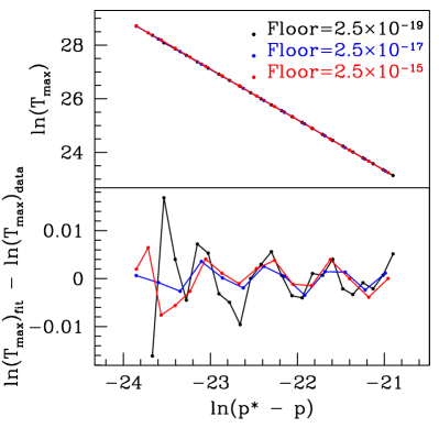
Figure 5.7: The scaling behavior in $T_{\max}$ near the critical solution for runs using different values of $P_{\mathrm{floor}}$ and $\delta$. The black line connects data from the original configuration, while the blue and red data points are from runs using the significantly larger floor values listed in the upper-right of the plot. The scaling exponents $\gamma$ for these runs are listed in Table 5.2

The effect on the scaling behavior due to the fluid’s floor (Section 3.7) will be estimated first. Since the floor is employed merely to alleviate our numerical scheme’s inability to treat the fluid dynamics at the relative scale of numerical round-off and represents nothing physical, it is crucial to verify that any results obtained with such methods are independent of the magnitude of the floor. To test this, we replicated the “original” results shown in Figures 5.1- 5.3 using different values of the floor while keeping all other parameters fixed. Both $P_{\mathrm{floor}}$ and $\delta$ were increased by the same factor to keep their relative magnitudes the same. The scaling behavior obtained using these different floor values is illustrated in Figure 5.7. The blue and red lines correspond to floor values that are factors of $10^{2}$ and $10^{4}$, respectively, larger than the original configuration, which itself used $\delta=2.5\times 10^{-19}$ and $P_{\mathrm{floor}}=10^{3}\delta$. The minimal influence of the floor on solutions in the critical regime is clearly seen by the fact that all the points follow nearly the same best-fit line. In fact, Table 5.2 indicates that all estimated values of $\gamma$ agree to within $\simeq 0.5\%$ and that all estimates of $p^{\star}$ coincide to within $4\times 10^{-4}\%$. The deviations of the calculated sets $\{\ln\left(T_{\max}\right),\ln\left(p^{\star}-p\right)\}$ from their respective best-fit lines for the different floor values even follow the same functional form, suggesting that the observed “periodic” deviations from linearity are not due to the floor. The fact that the scaling behavior is hardly affected by differences in the floor at these magnitudes is not too surprising since the component of the fluid that undergoes self-similar collapse is never rarefied enough to trigger the floor’s use. For instance, at a time when the central part of the star begins to resemble an ultra-relativistic critical solution, the maximum values of $\{D,\Pi,\Phi\}$ are, respectively, $\{\sim 10^{2},\sim 10^{3},\sim 10^{3}\}$—far above the typical floors used. Only for $r\gtrsim R_{\star}$ will the floor be activated, and dynamics in this region cannot affect the interior solution once the self-similar collapse initiates due to the characteristic structure of near-critical solutions as described in Figure 3.4. From this figure we see that all the waves of the fluid are traveling outward once it escapes from the self-similarity region. Therefore, we see that the presence of an artificial definition of the fluid’s vacuum state has a negligible effect on the observed scaling behavior.

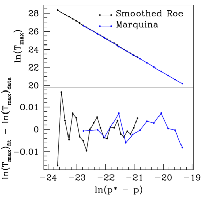
Figure 5.8: A comparison of the scaling behavior in $T_{\max}$ near the critical solution obtained with two different Riemann solvers. The “Smoothed Roe” line corresponds to runs made with the approximate Roe solver with a smoothing procedure outlined in Table 3.5; this distribution is also called “Original” or “$\mathrm{level}=0$” in other figures. The other line was generated using the Marquina method, with all other parameters fixed. The scaling exponents, $\gamma$, for these runs are listed in Table 5.2

Now we discuss the effect of the Riemann solver used on the scaling behavior. As mentioned in Section 3.11, an instability, which is apparently numerical in origin, forms at the sonic point of those solutions that have been tuned near the threshold of black hole formation. We found that the Marquina Riemann solver performs better than the approximate Roe solver without smoothing, so we wish to find out if it leads to the same $\gamma$ obtained using the Roe solver with smoothing enabled. From Figure 5.8, we see that the scaling behavior of $T_{\max}$ from the two methods is remarkably close. Even though the Roe method with smoothing allows us to determine $\ln\left(T_{\max}\right)$ for smaller values of $\ln\left(p^{\star}-p\right)$, the deviations from the best-fit of the two data sets are of the same order of magnitude for common values of $\ln\left(p^{\star}-p\right)$. From Table 5.2, we see that the respective values of $\gamma$ agree to within $0.3\%$ and that values of $p^{\star}$ agree to within $10^{-3}\%$. These differences are quite small—comparable to those found as a result of varying the floor. Hence, we may conclude that the choice in Riemann solvers has little, if any, effect on the computed scaling behavior, indicating that the smoothed approximate Roe solver is adequate for our purposes. It remains to be seen if, in fact, the instability is affected when using other Riemann solver, to see if the instability is not just an artifact of these two solvers.

Figure 5.9: The scaling behavior in $T_{\max}$ near the critical solution for runs using different levels of resolution. The runs were made with $\rho_{c}=0.05$, $U=U_{1}$, and the black line was generated from runs using the original configuration. The $\mathrm{level}=1,2$ runs, respectively, used computational grids that were locally $2$ times and $4$ times as refined. The scaling exponents, $\gamma$, for these runs are listed in Table 5.2

When using finite difference methods, it is vital to verify that the order to which the derivatives are approximated by difference operators is the same as the order of the solution error. For example, our HRSC scheme should be $O(\Delta r^{2})$ accurate in smooth region and $O(\Delta r)$ near shocks, so we should expect this scaling behavior of the error as $\Delta r$ is varied. First, we wish to see if our estimate for $\gamma$ converges as the grid is refined. Figure 5.9 shows a plot of $\ln\left(T_{\max}\right)$ versus $\ln\left(p^{\star}-p\right)$ for the original configuration (black) along with others computed at higher resolutions (blue and red). Please see Section 3.8.3 for a description on how the nonuniform mesh is refined. We first see that the three distributions follow lines shifted by a constant amount of approximately the same slope, while the deviation of the best-fits seems to increase slightly with resolution. Also, we can see that an increase in resolution allowed us to follow the collapse through to dispersal for solutions closer to the critical threshold, allowing for the scaling law to be sampled at smaller $\ln\left(p^{\star}-p\right)$. Even though the deviations from the best-fits for $l=1,2$ are quite small compared to the typical size of $\ln\left(T_{\max}\right)$, it is a little worrisome that they are larger than those from the lowest resolution runs. However, this increase can likely be attributed to the sonic point instability and the smoothing procedure used to damp it. In particular, the “hump” of the instability sharpens with increasing resolution spanning a roughly constant number of grid cells (see Section 3.11 for more details). Consequently, the instability’s impact on the solution may also increase with decreasing $O(\Delta r)$, since the discretized difference operators will—in turn—lead to larger estimates for spatial derivatives. In addition, the smoothing operation is always performed using nearest-neighbors, so the smoothing radius physically shrinks with resolution, diminishing the impact of the smoothing.

Figure 5.10: The logarithm of scaled, independent residuals of the Hamiltonian constraint (2.129) and slicing condition (2.130) for three levels of resolutions calculated from solutions in the self-similar regime. The blue (red) lines are from a run which used $2$ ($4$) times the local spatial and temporal resolutions of the original run, which represented by the black lines; the red residual was scaled by a factor of $16$ and the blue by $4$ in order to make the $O(\Delta r^{2})$ convergence of the solution more apparent. Each distribution is from a solution that has been tuned to $\ln\left(p^{\star}-p\right)\simeq-19$ with respect to each resolution’s value of $p^{\star}$. Every tenth grid point of each level’s distribution is displayed here. The physical velocity of the fluid for the $l=0$ run is shown in the bottom frame in order to facilitate comparison of features in the truncation error to those in the solution.

In order to verify that the code is converging in the self-similar regime, we computed the independent residuals of the Hamiltonian constraint (2.129) and slicing condition (2.130) for the three levels of resolution (Figure 5.10). The independent residuals used for the metric equations are given in Section 3.9. Each residual was first scaled such that they would all coincide assuming $O(\Delta r^{2})$ convergence; that is, the $l=2$ residuals were scaled by a factor of $16$ and the $l=1$ residuals were scaled by a factor of $4$. The overlap of residuals seen in the figure indicates $O(\Delta r^{2})$ convergence. Note that smoothing procedure has not been used to calculate the solutions shown here. We see that the scaled residuals follow similar magnitudes of smooth form in all regions except those which have been processed by shocks, namely $\mathcal{X}_{a}=[0,4.5],\simeq 7.8,\simeq 9.4$. Because the self-similar solutions are converging at the expected rate, we surmise that the variations observed in $\gamma$ for the three resolutions does not indicate a problem with convergence, but demonstrates the effect of truncation error on the scaling behavior. With only three levels of resolution, it is hard to make definite claims as to whether $\gamma$ is or is not converging to a particular value. Even so, the standard deviation of $\gamma$ determined from the three evolutions is about $1\%$ of their mean, suggesting that the observed variation in $\gamma$ values is not significant. In fact, the variation of $\gamma$ as a function of resolution is comparable to that found with the simpler ultra-relativistic perfect fluid [63]. In the convergence test performed, their values of $\gamma=0.9989,0.9837,0.9600$ were obtained for $l=0,1,2$, which suggests a relative standard deviation of $2\%$.

Figure 5.11: The scaling behavior in $T_{\max}$ near the critical solution for several “families” of initial data. The “Original” line was made from runs with $\rho_{c}=0.05$, $U=U_{1}$, and whose initial grid was made with the following parameters $\{N_{a},N_{b},N_{c},\mathrm{level}\}=\{300,500,20,0\}$. The blue line shows the scaling behavior for runs that used a different initial velocity profile, $U=U_{2}$. And, the red line was made from runs with a different TOV solution, defined by $\rho_{c}=0.531$. The scaling exponents, $\gamma$, for these runs are listed in Table 5.2

The final comparison we discuss entails varying the physical initial conditions of the system to investigate the universality of the critical phenomena computed with the ideal-gas EOS. The primary constituents of our model are the initial star solution and the form of the perturbation with which we drive the star to collapse. Hence, we chose to perform sets of runs to measure the scaling law using 1) a different initial star solution and 2) a different functional form of the initial velocity profile. The scaling behavior of $\ln\left(T_{\max}\right)$ versus $\ln\left(p^{\star}-p\right)$ for these different configurations are compared to the results from the original configuration in Figure 5.11. For the distribution found with a star specified by the central density $\rho_{c}=0.0531$ (red points), we kept everything else the same as that used in the original configuration except for the initial star solution. The blue points show data from runs that used $U_{2}$ (2.226) for the initial profile of the coordinate velocity. Naturally, we see that the three distributions are shifted from each other since each set evolved from significantly distinct profiles of mass-energy which obviously sets the scale for $T_{\max}$ at specific values of $p$. However, we are interested in the slopes of the curves which determine $\gamma$ for the particular systems.

From the values listed in Table 5.2, we see that $\gamma$ varies more significantly with the particular star solution used, than with the form of the velocity profile. In fact, we were able to tune closer to the critical solution with the more compact star, possibly because it required a smaller perturbation to enter the self-similar phase so that the global maximum of the Lorentz factor, $W$, was smaller for the same relative point in the tuning process or same $\ln\left(p^{\star}-p\right)$. We actually observe that the global maximum of $W$ for the most nearly critical solutions in both cases was $\sim 10^{6}$ even though the $\rho_{c}=0.0531$ solution was tuned significantly closer to criticality. Nonetheless, the different star’s scaling exponent agrees with the original’s to an accuracy of $2\%$.

The change in the function used for the initial velocity profile hardly affected the computed value of $\gamma$. The deviation in $\gamma$ found for the two profiles is surprisingly small: $0.04\%$. Thus, we find that the initial form profile has very little to do with the observed scaling exponent. This suggests that other methods of perturbation would also yield close to the same value. These three different families of initial data imply that universality of critical solutions is maintained for perfect fluids of given $\Gamma$ that follow the ideal-gas EOS. It would be interesting to see whether these results are maintained with even more realistic equations of state.

5.1.2 Final Determination of $\gamma$

Using the calculated values of $\gamma$ from the various methods, floor sizes and grid resolutions, we are able to provide an estimate of the systematic error inherent in our numerical model. Further, by assuming that the universality is strictly true, we can even use the variation for the different families used in this estimation. Taking the average and calculating the standard deviation from these values for the ideal-gas EOS given in Table 5.2, we find that our value of the exponent is

$$\gamma\ =\ 0.94\pm 0.01\quad.$$ (5.6)

This is in agreement with $\gamma$ from the black hole mass scaling fit Figure 5.2.

Method	$\rho_{c}$	$\delta$	$l$	$U$	$\gamma$	$p^{\star}$
Roe	0.05	$2.5\times 10^{-19}$	0	$U_{1}$	0.94	0.4687536738
Roe	0.05	$2.5\times 10^{-17}$	0	$U_{1}$	0.94	0.4687535028
Roe	0.05	$2.5\times 10^{-15}$	0	$U_{1}$	0.95	0.4687516089
Roe	0.05	$2.5\times 10^{-19}$	1	$U_{1}$	0.92	0.4682903094
Roe	0.05	$2.5\times 10^{-19}$	2	$U_{1}$	0.93	0.4682461196
Roe	0.05	$2.5\times 10^{-19}$	0	$U_{2}$	0.94	0.4299031509
Roe	0.0531	$2.5\times 10^{-19}$	0	$U_{1}$	0.92	0.44820474298
Marquina	0.05	0	0	$U_{1}$	0.94	0.46876822118
Ultra-rel.					0.97

Table 5.2: The scaling exponents $\gamma$ and critical parameters $p^{\star}$ from fits to the expected scaling behavior in $T_{\max}$. The runs labelled “Roe” use the approximate Roe solver with smoothing, the “Marquina” run used the Marquina flux formula instead, and the “Ultra-rel.” scaling exponent was computed from our results involving the collapse of Gaussian profiles of ultra-relativistic fluid.

In addition, we can compare our final estimate of $\gamma$ to values previously found for the ultra-relativistic fluid. As already mentioned, Neilsen and Choptuik [63] measured $\gamma$ at three different refinement levels, and quoted a value

$$\gamma_{NC}\ \lesssim\ 0.96\quad.$$ (5.7)

Instead of solving the full set of PDE’s, $\gamma$ can also be found by solving the eigenvalue problem that results from performing $1^{\mathrm{st}}$-order perturbation theory about the CSS solution. This was done in two ways by [10]: using the common shooting method, and solving the linear system directly after differencing the equations to $2^{\mathrm{nd}}$-order. The scaling exponents calculated were, respectively, $\gamma=0.9386\pm 0.0005$ and $\gamma=0.95\pm 0.01$.

We find our value (5.6) to agree well with those found by [10], and agree with $\gamma_{NC}$ to within the uncertainty quoted by Neilsen and Choptuik. The discrepancy between the value from the ideal-gas equations and that determined from the ultra-relativistic PDE’s is also seen when we solve the ultra-relativistic equations. Our ultra-relativistic value, $\gamma=0.97$, agrees well with those calculated by Neilsen and Choptuik, but deviates by 3 standard deviations from our ideal-gas calculations. It somewhat interesting, yet possibly coincidental, that our results from the ideal-gas system of equations lead to estimates of $\gamma$ that agree with the perturbation calculations better than those values found from the ultra-relativistic PDE calculations.

Hence, some of the claims made by Novak [66] have been found to be significantly inaccurate for the ideal-gas EOS with $\Gamma=2$. It remains to be seen whether the scaling behavior we have observed is also seen with more realistic state equations such as the one Novak used [69]. Since accurate measurements of $\gamma$ have only been found for equations of state with constant adiabatic indexes $\Gamma$, and since $\gamma$ seems to only depend on $\Gamma$ for perfect fluids, it remains to be seen what the scaling behavior—if any—will be like for realistic state equations that do not guarantee that $\Gamma$ be constant throughout the fluid.

5.2 Type II Phenomena with Scalar Field Perturbation

It is important to mention that we had been studying perturbed neutron stars before [66] was published. Instead of using an initial velocity, however, a minimally-coupled, massless scalar field was used to perturb the star purely through their mutual gravitational interaction. That is, the energy of the scalar field leads to spacetime curvature to which the star responds, and vice versa. In order to search for critical phenomena, we tuned the magnitude of the initial Gaussian shell of scalar field about the threshold of black hole formation. Type I behavior was studied extensively with this multi-matter system, and is described in Chapter 6. Surprisingly, we were unsuccessful in driving the star’s matter to CSS collapse with the scalar field perturbation. Those stars which did not follow Type I behavior were sparser and less massive, requiring a larger excitation to collapse. The scalar field profile needed to collapse the star was sufficiently strong that it exhibited Type II behavior itself instead of merely perturbing the star. That is, when the scalar field profile was tuned about the critical point, we found that the near-threshold solution was the scalar field DSS solution found in the first critical phenomena study [19].

Figure 5.12: A snapshot of the separate contributions to the energy density from the massless scalar field and from the fluid for Type II collapse involving a coupling of the two fields. This particular frame shows the configuration just prior to black hole formation for the most nearly critical solution. The scalar field contribution is shown in blue while the fluid contribution is shown in black. The two are plotted against a self-similar coordinate $\mathcal{X}_{a}$ which tracks the maximum of the metric function $a$ (2.65). The star shown here corresponds to $\rho_{c}=0.02$ and $\Gamma=2$. Every fifth grid point is shown here for each distribution.

For example, Figure 5.12 shows the scalar field and fluid contributions to $dm/dr$ (2.196) for a Type II collapse with the massless scalar field and star. The scalar field and fluid contributions are, respectively,

$$\frac{d}{dr}m_{\,{}_{\mbox{\scriptsize$\mathrm{scalar}$}}}\ =\ 4\pi r^{2}\varrho_{\,{}_{\mbox{\scriptsize$\mathrm{scalar}$}}}\quad,\quad\frac{d}{dr}m_{\,{}_{\mbox{\scriptsize$\mathrm{fluid}$}}}\ =\ 4\pi r^{2}\varrho_{\,{}_{\mbox{\scriptsize$\mathrm{fluid}$}}}$$ (5.8)

where $\varrho_{\,{}_{\mbox{\scriptsize$\mathrm{scalar}$}}}$ and $\varrho_{\,{}_{\mbox{\scriptsize$\mathrm{fluid}$}}}$ are given in (2.195) and (2.194). The periodic echoing of the scalar field’s DSS collapse can be clearly seen in the oscillations of $dm_{\,{}_{\mbox{\scriptsize$\mathrm{scalar}$}}}/dr$ for $\mathcal{X}_{a}>0$. The presence of the oscillations in this late-time snapshot illustrates how the non-self-similar part of the fluid “freezes out”, or evolves at an exponentially slower rate than the interior part of the solution; in this way, the spatial profile of the distributions serve as a sort of historical record of the collapse. Also, it appears that the fluid reacts to the echoing of the spacetime, indicated by the periodic discontinuities in $dm_{\,{}_{\mbox{\scriptsize$\mathrm{fluid}$}}}/dr$ that occur at $\mathcal{X}_{a}=3,6,10$. Especially interesting, though, is that the echoing of the scalar field contribution occurs twice as frequently as the fluid’s. From the evolution of the fluid velocity $v(r,t)$ and the discontinuities in this figure, we see that shocks seem to develop at every other echo. In addition, the disparate magnitudes of $dm_{\,{}_{\mbox{\scriptsize$\mathrm{scalar}$}}}/dr$ and $dm_{\,{}_{\mbox{\scriptsize$\mathrm{fluid}$}}}/dr$ demonstrate how irrelevant the fluid is in this region of spacetime. We may conclude, then, that the fluid was a passive element as the scalar field—and the spacetime it dominated—collapsed in a discretely self-similar fashion.

The next chapter contains further discussion regarding the dynamics of a massless scalar field coupled to neutron star models through their gravitational interaction.

Chapter 6 Type I Critical Phenomena

Compared to Type II phenomena in general relativity, Type I behavior is far simpler to study in many respects and involves systems that are not quite as exotic as the Type II variety. Instead of the critical solutions having self-similar symmetry, Type I critical solutions have always been found to exhibit continuous (static) or discrete (oscillatory) symmetry with respect to time. In this chapter, the first thorough study of Type I behavior of perfect fluid solutions is presented. Other Type I studies have involved a great variety of other field theories. For example, the first model in which Type I behavior was explored was the self-gravitating SU(2) gauge field, or Einstein-Yang-Mills (EYM) system, [24]. In this work, Choptuik et al. found that the threshold solution of certain EYM systems is the static $n=1$—where $n$ parameterizes the number of zero-crossings of the Yang-Mills field—Bartnik-McKinnon solution [5] which has one unstable mode. Next, Brady et al. [9] were the first to discover Type I collapse involving an oscillating critical solution in their study of a real massive scalar field coupled to gravity. The critical solutions they found belong to the class of oscillating solitonic solutions constructed by Seidel and Suen [78]. In these studies, the two “fixed points” in phase space involve either a black hole or flat space (vacuum). However, in the Einstein-Skyrmion model, whose Type I behavior was first examined by Bizon and Chmaj [8], the non-black hole fixed point is one containing a stable, static Skyrmion solution. After approximating the unstable static solution for some time, the near-critical Skyrmion field would either form a black hole or expand to a stable, equilibrium solution.

Possibly the most similar study to ours was done by Hawley and Choptuik [43]. They investigated perturbed stable boson star solutions, which are massive complex scalar field solutions whose only time-dependence is a phase that varies linearly with time. In order to perturb the stable boson stars, they collapsed a spherical pulse of massless scalar field onto it from a distance far outside the star’s radius, to ensure that the two distributions were initially distinct. As the pulse collapses through the origin, the two energy distributions interact solely through the gravitational field. The increase in curvature within the star from the massless field was observed to be enough to drive the boson stars inward, resulting in either black hole formation or a sequence of large oscillations. Note that in the original paper by Hawley and Choptuik [43], they did not find that the subcritical fixed point involved a periodic spacetime, but assumed that the stars would disperse to spatial infinity. Upon evolving subcritical evolutions longer, Lai [50] found that they were, in fact, bound and oscillatory systems. Later, Hawley [44] confirmed these results. During the non-trivial gravitational interaction of the massless scalar field and the boson star, a transfer of mass-energy from the massless scalar field to the complex scalar field was observed, increasing the gravitating mass of the boson star. Type I critical solutions were found by varying the magnitude of the initial pulse of massless scalar field, and it was shown that the critical solutions were unstable boson star solutions with masses somewhat larger than their stable progenitors. Boson stars are similar to their hydrostatic analogues in that their stable solutions are on the branch below the maximum of $M_{\star}(\phi(0))$ graph, while the unstable solutions are on the other side (see Section 2.4 for a discussion regarding the hydrostatic star solutions). Finally, as with any Type I phenomena investigation, Hawley and Choptuik found that the lifetime of a solution tuned close to the threshold scales as a power-law of the deviation of the tuning parameter, $p$, from the critical value, $p^{\star}$:

$$T_{0}(p)\propto-\sigma\ln\left|p-p^{\star}\right|$$ (6.1)

They verified that the scaling exponent, $\sigma$, for a given critical solution is the inverse of the real part of the Lyapunov exponent, $\omega_{Ly}$, for the corresponding unstable boson star solution. They calculated $\omega_{Ly}$ for several cases using the ODE’s resulting from linear perturbation theory about the unstable solutions. Since boson stars model many of the characteristics of TOV solutions, it was conjectured that the critical behavior they discovered would carry over to their fluid analogues. We will see shortly that in many respects it does.

Before proceeding to the presentation of results, we would like to first mention that the threshold between hydrostatic solutions and black hole formation has been studied in a variety of ways in the past. For instance, the first time-dependent numerical simulations of a fully-coupled general relativistic system involved the collapse of adiabatic perfect fluid spheres of constant density and were performed by May and White in 1966 [59] (see [58] for a more thorough explanation of the methods used by May and White and see the work by Misner and Sharp [60] for the origin of the formulation they used). About five years later, Wilson [94] studied the core collapse supernova problem using an approximate method for the neutrino transport in full, spherically-symmetric general relativity. Van Riper in 1979 [90] studied the purely hydrodynamic collapse of iron core models of different masses in order to determine the maximum mass for the resultant neutron star. Interestingly enough, he tuned this critical mass to within $0.005\%$, but the “critical” or threshold solution he found never reached densities above the Oppenheimer-Volkoff limit, above which the TOV solutions become unstable.

Recently, Siebel et al. [82] sought to measure the maximum neutron star mass allowed by the presence of a perturbing pulse of minimally-coupled, massless scalar field. A general relativistic hydrodynamic code using a characteristic formulation was used to investigate the spherically symmetric system. Instead of varying the massless scalar field, however, they studied five star solutions of assorted central densities that straddled the threshold of black hole formation. They found that the perturbation either led to a black hole or to oscillations of the star about its initial configuration. Further, in order to test their new 3-dimensional general relativistic fluid code, Font et al. [33] dynamically calculated the fundamental and harmonic mode frequencies of spherical TOV solutions that were perturbed only by their initial truncation error. In this fashion, they were able to observe the transition of a TOV solution on the unstable branch to the stable branch by evolving the unstable solution with only a truncation error level perturbation. The expansion of the unstable star initially overshoots the stable solution, resulting in a series of oscillations.

6.1 Model Description

As others have done [43, 82], we chose to use a minimally-coupled, massless Klein-Gordon (EMKG) field to perturb our star solutions dynamically. The EMKG field is advantageous for several reasons. First, the fact that the two matter models are both minimally-coupled to gravity with no explicit interaction between the two ensures that any resulting dynamics from the perturbation is entirely due to their gravitational interaction. Second, the EOM of the EMKG field are straightforward to solve numerically and provide little overhead to the hydrodynamic simulation. Third, since gravitational waves cannot exist in spherical symmetry and the EMKG field only couples to the fluid through gravity, it can serve as a plausible first approximation to gravitational radiation acting on these spherical stars.

We will continue to approximate neutron stars as polytropic solutions of the TOV equations with $\Gamma=2$; and the factor in the polytropic EOS (2.221) will still be set to $K=1$ to keep the system unit-less. Since all stellar radii $R_{\star}$ satisfy $R_{\star}<1.3$ for such solutions, we will—by default—position the initial scalar field pulse at $r=5$. This has been found to be well outside any star’s extent and so ensures that the two models are not initially interacting and thus represent two independent distributions of energy at $t=0$.

6.2 The Critical Solutions

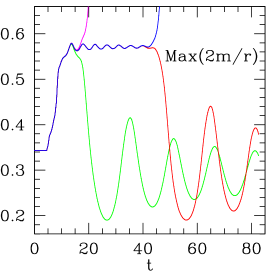
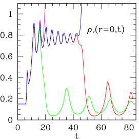
Figure 6.1: Evolutions of ${\max}(2m/r)$ and $\rho_{\circ}(r\!\!=\!\!0,t)$ from $4$ solutions near the threshold of a star parameterized by $\Gamma=2$, $\rho_{c}=0.15$. The purple (green) line is from a solution far from the threshold on the supercritical (subcritical) side. The blue (red) line pertains to a supercritical (subcritical) solution whose parameter has been tuned to within machine precision of the critical value.

The evolution of the star towards the critical solution and the critical solutions themselves will be described in this section. As the scalar field pulse travels into the star, the star undergoes a compression phase whereby the exterior implodes at a faster rate than the interior. This is reminiscent of the velocity-induced shock-bounce scenarios described in Chapter 4. If the perturbation is weak, then the star will undergo oscillations with its fundamental frequency after the scalar field disperses through the origin and finally escapes to null infinity (higher harmonics are also excited). On the other hand, when the initial scalar shell of sufficiently large amplitude, the star can be driven to prompt collapse, trapping some of the scalar field along with the entire star in a black hole. Somewhere in between, the scalar field can compactify the star to a nearly static state that resembles an unstable TOV solution of slightly increased mass. The length of time the perturbed star emulates the unstable solution, which we will call the lifetime, increases as the initial pulse’s amplitude is adjusted closer to the critical value, $p^{\star}$. It is expected from this scaling behavior that a perfectly constructed scalar field pulse with $p=p^{\star}$ would perturb the star in such a way that it would resemble the unstable solution forever. This putative infinitely long-lived state is referred to as the critical solution of the progenitor star.

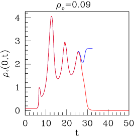
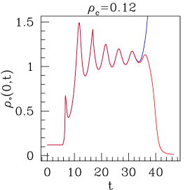
Figure 6.2: Sample evolutions of the central rest-mass density for supercritical (blue) and subcritical (red) solutions from progenitor stars with $\rho_{c}=0.09$ and $\rho_{c}=0.12$. The solutions have been tuned to within machine precision of criticality in each case. Note that for $\rho_{c}=0.09$, $\rho_{\circ}(0,t)$ for the supercritical calculation tends to a constant value since the collapse of the lapse has effectively frozen the star’s evolution near the origin. Also, even though it may seem from the figures that the subcritical solutions for both stars evacuate the origin, both inflate to larger, sparser star solutions along the lines of the shock-bounce-oscillate (SBO) scenario described in Section 4.1.

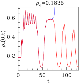
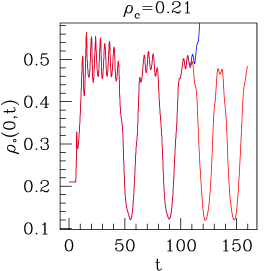
Figure 6.3: Further examples of the central density variation over time for the most nearly critical solutions from two stars, $\rho_{c}=0.1835$ and $\rho_{c}=0.21$; again, the subcritical solutions are plotted in red, while the supercritical solutions are plotted in blue. The $\rho_{c}=0.1835$ star is the star with the smallest initial central density whose nearest-to-critical solution exhibits a momentary departure from the unstable, equilibrium solution; this is indicated by the break between the two “plateaus” in the graph. This behavior is seen for most stars above $\rho_{c}=0.1835$, as exemplified by the other star’s solutions. The $\rho_{c}=0.21$ star is the sparsest initial solution found whose most nearly critical solutions have two departures or three plateaus.

Examples of solutions near and far from the critical solution are illustrated in Figure 6.1 for a star with $\rho_{c}=0.14$. Here we show the evolution of the spatial maximum of $2m/r$, ${\max}(2m/r)$, and the central density of the star for a series of solutions. The quantity $2m/r$ is, effectively, a measure of the degree of compactification; the global maximum that $2m/r$ can attain for the static TOV solutions studied herein is approximately $0.61$, and $2m/r\rightarrow 1$ when a black hole would form. The purple lines clearly show that the supercritical systems far from the threshold quickly collapse to black holes, represented here by the divergence of the central density and compactification factor. On the opposite side of the spectrum, we see from the periodic nature of the green ${\max}(2m/r)$ and $\rho(0,t)$ distributions that subcritical solutions undergo a series of oscillations. The blue and red lines, respectively, illustrate the long lifetimes of marginally supercritical and subcritical solutions. The plateau shown in the plots represents the period of time during which the marginally subcritical and supercritical solutions resemble the critical solution. We will see shortly that this critical solution is actually a star-like configuration oscillating about an unstable TOV solution.

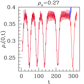
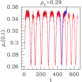
Figure 6.4: The central density evolutions from solutions tuned within machine precision for progenitor stars $\rho_{c}=0.27$ and $\rho_{c}=0.29$. These stars are close to the maximum mass equilibrium solution, $\rho_{c}=0.318$. The supercritical solutions are plotted in blue, and the subcritical solutions are shown in red. The nearest-to-critical solutions from the $\rho_{c}=0.27$ star shows four departures, while those from the $\rho_{c}=0.29$ star shows five. The supercritical solution from the $\rho_{c}=0.29$ initial star undergoes a curious sequence not seen in many cases—after it deviates from the subcritical solution—instead of collapsing to a black hole from the unstable, equilibrium configuration, it departs from it one last time only to return again, and then collapses.

Figure 6.5: Time series of fluid and scalar field contributions to $dm/dr$ for the most nearly critical solutions corresponding to the $\rho_{c}=0.197$ star. The supercritical (subcritical) fluid contribution is colored blue (red), and the scalar field contribution for the supercritical (subcritical) solution is green (cyan); the dotted black line is $dm/dr$ of the unstable, equilibrium solution that most closely approximates our critical solution. The elapsed time of each frame is shown in the upper-right corner. Since the differences between the supercritical and subcritical scalar field perturbations is on the order of machine precision, the subcritical scalar field contribution is completely obscured by the supercritical one. Indeed, the supercritical and subcritical fluid contributions are nearly identical until $t=80$, when the two solutions begin to diverge from the critical solution. In every frame, only every tenth grid point is displayed for each distribution.

Instead of dispersing to spatial infinity as do the solitonic oscillon stars of [9], the marginally-subcritical TOV stars ultimately settle into bound states. Depending on the magnitude of $p^{\star}$ for a particular progenitor star, the final star solution will either be larger and sparser than the original (large $p^{\star}$), or it will oscillate indefinitely about the original solution. In reality, the star will radiate away the kinetic energy of the oscillation via some viscous mechanism. In our model, however, the only dissipation is the trivial amount from the numerical scheme, and that from the star shock-heating its atmosphere—transferring the kinetic energy of the bulk flow into internal energy. If the subcritical star settles to a sparser solution, it will do this through a series of violent, highly-damped oscillations similar to the SBO scenarios of velocity-perturbed stars described in Section 4.1. Examples of such subcritical SBO solutions are depicted in Figures 6.1- 6.2. The damped oscillations are best illustrated in the marginally subcritical solutions shown in Figure 6.1, since the oscillations of the subcritical solution of $\rho_{c}=0.09$ occur at an imperceptible scale and those of $\rho_{c}=0.12$ occur at later times than are shown in Figure 6.2.

For these less relativistic and sparser stars, the perturbation required to generate near-critical evolution is quite large and, consequently, is such that it drives the star to significantly overshoot the unstable TOV solution, setting it to ring about the unstable solution instead. This meta-stable ringing decreases with decreasing $p^{\star}(\rho_{c})$, or increasing $\rho_{c}$. For instance, the critical solution of the $\rho_{c}=0.09$ star seems to correspond to an unstable TOV star with central density $\rho_{c}^{\star}\simeq 2$ that oscillates such that $0<\rho_{\circ}(0,t)<4$. The increase in central density—from the initial stable star to the unstable star solution—represents an increase by a factor of $22$. This is to be contrasted with the critical solution for the $\rho_{c}=0.29$ star which has a central density $\rho_{c}^{\star}\simeq 0.35$—an increase by a factor of $1.2$; this critical solution oscillates such that $0.32<\rho_{\circ}(0,t)<0.38$. This trend will be discussed further in the next section.

In addition to smaller oscillations about the meta-stable states for denser initial stars, we see from Figures 6.3- 6.4 that near-critical evolutions can momentarily depart from their meta-stable states. The departures are illustrated by a break in the plateaus of the $\rho_{\circ}(0,t)$ distributions. As $\rho_{c}$ increases and gets closer to the turnover point, which is located at $\rho_{c}=0.318$, we see that the number of distinct plateaus increases. The $\rho_{c}=0.1835$ solution is the smallest initial central density where two plateaus are observed, and $\rho_{c}=0.21$ is the first one where three are seen. For higher densities we see an ever-increasing number of plateaus, most likely because the difference between the progenitor solution and its corresponding critical solution is diminishing.

As we can see in the time sequence of the scalar field and fluid contributions to $dm/dr$ in Figure 6.5, the marginally subcritical and supercritical stars leave the unstable TOV star configuration only to return to it after one oscillation about the progenitor solution. The unstable star was found by taking the time average of $\rho_{\circ}(0,t)$ for the most nearly critical solutions as described in detail below. The shock from the outer layers of the star reacting first to the increase in curvature is first seen at $t=9$ of this figure, and the time referred to in this figure coincides with proper time at spatial infinity.

Figure 6.6: Illustration of the fitting procedure used to determine the central density of the critical solution, $\rho_{c}^{\star}$. The progenitor star corresponds to a star with $\rho_{c}=0.197$. The critical solution shown here exhibits two plateaus, and we calculate $\rho_{c}^{\star}$ from both plateaus. The time-spans used to calculate both averages are determined by the first and last peaks that seem to represent complete sets of oscillations for the unstable star. These periods of time are shown here by the solid, vertical lines. For instance, the last peaks on each plateau are significantly smaller than the other plateaus’ peaks suggesting that star has already begun its departure from the unstable solution.

Making a quantitative comparison of the critical solution to an unstable star is not easy since the critical solution is not exactly static. If we make the assumption that the oscillation is sinusoidal, we can take a time-average of the solutions when the critical solution most resembles an unstable star. Figure 6.6 graphically depicts how we go about this for for the $\rho_{c}=0.197$ critical solution as an example. We first start with the subcritical solution which is tuned closest to the critical solution. The periods at which the solution best approximates the unstable solution are determined by qualitatively judging where the sequences of quasi-normal oscillations begin and end for the unstable star. For instance, in this figure we can clearly see that that the “first” peak—located at $t\simeq 12$—of the first plateau does not “belong” to the sequence of quasi-normal oscillations since it is distinctly smaller than the “second” peak of this plateau. Thus, we start the time-average from this second peak and stop before the last peak since it, too, seems out-of-character with this particular sequence of oscillations. The central density, $\rho_{c}^{\star}$, of the unstable star solution corresponding to the critical solution is then calculated by taking the time-average of $\rho_{\circ}(0,t)$ over a given period. This is repeated for other plateaus if present, so Figure 6.6 would yield—for instance—two estimates of $\rho_{c}^{\star}$. For each system with multiple plateaus studied here, we have found the plateau averages all agree with each other to within their standard deviation. Hence, we feel that this is a consistent method for identifying the unstable star associated with a critical solution. The standard deviations of $\rho_{\circ}(0,t)$ for $\rho_{c}=0.197$ about its calculated $\rho_{c}^{\star}$ are represented by the red and blue sets of dashed lines, whereas the average for each plateau is given by a solid, horizontal line.

Figure 6.7: The time-average (blue crosses) of a marginally subcritical solution compared to the unstable TOV solution (black line) it best approximates. The time-average was performed while the solution dwelled on the second plateau, shown in Figure 6.6. The unstable star was calculated by numerically solving the TOV equations using $\rho_{c}^{\star}$ for as the solution’s central density. The distributions shown in red, whose ranges are given on the right-hand sides of the plots, are the point-wise differences between the other two functions plotted. The solutions and their deviations are only shown here within the stellar radius, $R_{\star}$.

After identifying a perturbed star’s associated unstable solution, its shape with the solution it oscillates about during a plateau. To perform this comparison for $\rho_{c}=0.197$, we first took the time-average of the perturbed star during the second plateau. This time-average serves as an approximation to the static solution about which the critical solution varies, assuming that the deviations are sinusoidal in nature. The time-averaged solution can then be compared to the TOV solution with central density $\rho_{c}^{\star}$. The results of this comparison for the critical solution of the $\rho_{c}=0.197$ perturbed star are shown in Figure 6.7. Metric and fluid functions from the time-average (black) and the estimated unstable TOV solution (blue) are shown together along with their differences (red). This figure clearly shows that, during “plateau epochs”, the critical solution closely approximates that of an unstable TOV solution of the same central density. The relative deviation between the two solutions increases near the radius of the star, $R_{\star}$, which is not surprising since the fluid’s time-averaged velocity is greatest there. Also, near $R_{\star}$ the star is most likely interacting with the atmosphere in a non-trivial way, which could alter its form near its surface. In fact, a similar discrepancy was observed in the critical boson star solutions in [43]; they found that the critical solutions had a longer “tail” than their corresponding static solutions. Still, the differences we see here are encouraging, and suggest strongly that the critical solutions we obtain are perturbed stellar solutions from the unstable branch.

6.3 Mass Transfer and the Transition to the Unstable Branch

Not only does the perturbing scalar field momentarily increase the spacetime curvature near the origin as it implodes through the star, the gravitational interaction of the two matter fields involves an exchange of mass from the scalar field to the star. A hint of this was shown in Figure 6.5 by the difference in heights of $dm_{\mathrm{scalar}}/dr$ before and after the interaction. In Figure 6.8, we provide a more explicit illustration of the mass exchange for two marginally subcritical solutions of stars with $\rho_{c}=0.197$ and $\rho_{c}=0.09$. The figure shows the mass contributions for each matter component, as well as, the total gravitating mass. $M_{\mathrm{total}}$ is calculated via (2.38), while $M_{\mathrm{fluid}}$ ($M_{\mathrm{scalar}}$) is found by integrating $dm_{\mathrm{fluid}}/dr$ ($dm_{\mathrm{scalar}}/dr$) from the origin to the outer boundary. For each case, the non-trivial gravitational interaction of the fluid and scalar field can be recognized by the sudden change in their integrated masses, which occurs near $t=7$ in each plot. The perturbation for the $\rho_{c}=0.197$ star is small and does not transfer a significant portion of its mass to the star, whereas the perturbation required to drive the $\rho_{c}=0.09$ star to its marginally subcritical state transfers more than an third of its mass to the star before leaving the bounds of the star. This dramatic interaction drives the star to oscillate wildly about its unstable counterpart—as seen in Figure 6.2—and it eventually expels a great deal of its mass as it departs from this highly energetic, yet unstable, bound state. The slow leaking of the ejected matter from the grid is clearly seen in Figure 6.8 as the long tail of $M_{\mathrm{fluid}}/M_{\mathrm{total}}$ that starts well after the scalar field leaves the grid.

Figure 6.8: The integrated masses of the matter fields as a function of time for marginally subcritical solutions and progenitor stars with $\rho_{c}=0.197$ and $\rho_{c}=0.09$. The decrease in $M_{\mathrm{total}}$ at the same time as $M_{\mathrm{scalar}}$ vanishes signifies the scalar field leaving the numerical grid; from the time it leaves, $M_{\mathrm{total}}=M_{\mathrm{fluid}}$.

Figure 6.9: Mass versus the log of the central density for equilibrium solutions (solid black line), a few of the initial data sets used (green dots), and the critical solutions obtained from this initial data sets (blue and red dots). The central densities of the critical solutions are obtained by taking a time average of the central density when the star is in resembling the critical solution. The blue dots refer to equilibrium solutions with central densities that match those of the critical solutions, while we have used the mass of all the fluid in the numerical domain in determining the locations of the red and green dots. The red and blue lines match the initial solutions to their critical solutions.

To examine how the amount of mass exchange varies for different critical solutions and to see where exactly critical solutions fall on the $M_{\star}$ versus. $\rho_{c}$ graph of equilibrium solutions, we construct Figure 6.9. The initial star solutions are indicated here on the left side—the stable branch—-while their critical solutions are shown on the right near the unstable branch. The central densities of the red and blue dots use the values of $\rho_{c}^{\star}$ calculated by fitting $\rho_{\circ}(0,t)$ during periods when the star emulates the critical solution, as described in the previous section. Only the masses of the blue and red dots vary; masses of the blue solutions are those corresponding to the unstable TOV solutions with central density equal to $\rho_{c}^{\star}$, and the masses of the solutions represented by the red dots are $M_{\mathrm{fluid}}$ calculated after the scalar field has left the numerical domain. The amount of mass transferred to a particular star from the scalar field is represented here by the mass difference of the red and blue dots corresponding to the same $\rho_{c}$. We can see that the total fluid mass is always larger than its initial mass, whereas the mass of the critical solution’s associated unstable star solution is always smaller than its stable progenitor. In addition, as the turnover is approached, both of these deviations diminish until, at turnover, the final mass of the fluid distribution corresponds to its initial mass and the mass of the unstable TOV solution.

The fact that the unstable TOV solution is always smaller than the progenitor may be explainable in a number of ways. First, the oscillations of the critical solution about the unstable star configuration may not be sinusoidal, thereby leading to central density estimate that is possibly larger than it should be. A larger central density would then lead to a mass estimate that is less than it should be, since $dM_{\star}/d\rho_{c}<0$ on the unstable branch. Second, it was seen in Figures 6.2- 6.4 that the oscillations of the critical solutions decrease with increasing $\rho_{c}$. The decrease in the amount of energy in these kinetic modes seems to be correlated with the decrease in the exchanged mass. It is most certainly the case that a large portion of exchanged mass goes into perturbing the unstable star solution.

6.4 Type I Scaling Behavior

As the initial pulse of scalar field is adjusted toward $p^{\star}$, the lifetime of the meta-stable, near-critical configuration increases. To quantify the scaling for a given initial star solution, the subcritical solution closest to the critical one is first determined. This is done by tuning the amplitude of the scalar field pulse, $p$, until consecutive bisections yield a change in $p$ smaller than machine precision. Let $p^{\mathrm{lo}}$ be the value of $p$ that yields the subcritical solution that most closely approximates the critical solution. For each $p$, a unique solution is produced that resembles this marginally subcritical solution for different lengths of time, determined by how close $p$ is from $p^{\star}$. Assuming that the $p^{\mathrm{lo}}$ solution resembles the critical solution longer than any other from our code, the lifetime, $T_{0}(p)$, is then determined from the proper time measured at the origin that elapses until

$${\max}(2m/r)[T_{0}(p),p]-{\max}(2m/r)[T_{0}(p),p^{\mathrm{lo}}]\ >\ 0.01{\max}(2m/r)[T_{0},p^{\mathrm{lo}}]$$ (6.2)

where ${\max}(2m/r)[T_{0}^{\prime},p]$ is the value of ${\max}(2m/r)$ at central proper time $T_{0}^{\prime}$ for the solution specified by $p$. This lifetimes are then plotted against the natural logarithm of the deviation of $p$ from $p^{\star}$ to find the scaling exponent from the expected trend (6.1). An example of a linear fit to such values is given in Figure 6.10. Since supercritical solutions resemble the critical solution as well as subcritical solutions, then both kinds can be used when determining the scaling exponent $\sigma$. The exponent is then found to be the negative of slope of the line. The deviation of the code-generated data from the best-fit has an obvious modulation, most likely due to the periodic nature of the critical solution.

Figure 6.10: The lifetimes, $T_{0}(p)$, for solutions near the critical solution for a $\rho_{c}=0.14$ star. The scaling exponent, $\sigma$, is found from the negative of the slope of the best linear fit to the points. The fact that both supercritical and subcritical solutions can be used for calculating $T_{0}(p)$ is illustrated here by our inclusion of both sets of points: the blue points show data from supercritical solutions and the red points come from subcritical calculations. The lifetimes here are actually those as measured at spatial infinity; see the text for further information.

In practice, the lifetime is determined using the proper time elapsed at spatial infinity, $T_{\infty}$, instead of that measured at the origin. In order to get the correct scaling exponent, which would correspond to $1/\omega_{Ly}$ of the unstable mode, $\sigma_{\infty}$ must be rescaled. Since $T_{\infty}$ is the same as our coordinate time, $t$, then

$$dT_{0}(t)=\alpha(0,t)\,dt\quad.$$ (6.3)

In order to estimate the rescaling factor, we assume that $\alpha(0,t)$ does not vary much when the solution is in the near-critical regime, so that

$$\alpha(0,t)\approx\alpha^{\star}(0)$$ (6.4)

where $\alpha^{\star}$ is the central value of the lapse of the unstable TOV solution that corresponds to the critical solution. The corrected value of $\sigma$ is then calculated using:

$$\sigma=\alpha^{\star}\sigma_{\infty}\quad.$$ (6.5)

We have performed fits for $\sigma_{\infty}$ and then rescaled them using the above procedure to obtain an estimate of $\sigma$ for $55$ different initial TOV stars. The variation of $\sigma$ with $\rho_{c}^{\star}$ is shown in Figure 6.11. We find that $\sigma(\rho_{c}^{\star})$ fits surprisingly well by the linear relationship

$$\sigma=5.93\rho_{c}^{\star}-1.475\quad.$$ (6.6)

In order to verify that the calculated $\sigma$ values are, indeed, equal to $1/\omega_{Ly}$, we would need to calculate the fundamental modes of the unstable star solutions. To the extent of my knowledge and others [54, 83], this has not been done before for the particular EOS used, and we leave this for future work.

Figure 6.11: The real part of the estimated Lyapunov exponent for a given star solution parameterized by $\rho_{c}^{\star}$. The black dots were calculated from data from the first “plateau”, while the blue dots from the second. ${\max}(2m/r)$ was used to calculate the $\omega_{Ly}$ shown here.

6.5 The Plateaus

In order to gather a better understanding of what causes the critical solutions to temporarily depart from the unstable branch, we performed a series of bisection searches for different values of various control parameters of our numerical simulations. For instance, to see if the presence of the departures is affected by changes in the floor, we tuned to the critical solution for three different sets of values for $\{\delta,P_{\mathrm{floor}}\}$. The most marginally subcritical solutions from these searches are shown in Figure 6.12. In addition, the effect of the outer boundary’s location, $r_{\max}$ is seen in Figure 6.13. To see if the time at which the pulse collides with the star has any effect, the initial position of the pulse, $R_{\phi}$ was varied; the results from this particular analysis are shown in Figure 6.14.

In general, we see all these aspects to have significant and non-trivial effect on the critical solution’s departure from the unstable solution. But, all the different marginally-subcritical solutions finally depart from the unstable solution at approximately the same time.

Whether because of its magnitude or extent, the solution’s departure seems to be affected by the floor. Increasing the size of the floor seems to hasten the initial departure; even though they represent only two points of reference, the similarity of the solutions with the two highest floor values may suggest that the floor’s effect “converges” to one behavior as its size increases.

On the other hand, changes in the size of the computational domain and $R_{\phi}$ seem to have no consistent effect on the first departure time.

The exact cause of these departures remains unsolved, and is left for future examination.

Figure 6.12: Comparisons of $\rho_{\circ}(0,t)$ for the marginally subcritical solutions obtained when using varying values of the fluid’s floor. The original, reference solution is shown in black and used $P_{\mathrm{floor}}=3.8809\times 10^{-15}$, $\delta=3.8809\times 10^{-18}$. The red and blue lines are from critical searches that used floor values $10$ and $100$ times greater, respectively, than those of the original solution. Variations can be seen between each floor size, even though this difference is smallest between solutions with the larger floor quantities. The star’s initial central density was $0.197$ for all the runs shown here.

Figure 6.13: The central density as a function of time of the most nearly critical, subcritical solutions obtained with physical domains of various sizes. The red (blue) sequence used a domain twice (thrice) as large as that of the original configuration, which is shown here by the black line. The star’s initial central density was $0.197$ for all the runs shown here.

Figure 6.14: The central density as a function of time of the most nearly critical, subcritical solutions obtained by using different initial locations of the initial scalar field distribution, $R_{\phi}$. Specifically, the scalar field at $t=0$ takes the form of a Gaussian distribution, and the position of the center of this Gaussian is unique for each color shown here. In the units used for these runs, the radius of the progenitor star was $r=0.87$, while the initial positions of the scalar field pulses were located at $r=4$ (red), $r=5$ (black), $r=6$ (blue), $r=7$ (green). The star’s initial central density was $0.197$ for all the runs shown here.

Chapter 7 Conclusion

In this work, we simulated spherically-symmetric relativistic perfect fluid flow in the strong-field regime of general relatively. Specifically, a perfect fluid that admits a length scale, for example one that follows a relativistic ideal gas law, was used to investigate the dynamics of compact, stellar objects. These stars were modeled as neutron stars by using a stiff equation of state, approximating the behavior of some realistic state equations. These models were then used to study the dynamics of neutrons so far out of equilibrium that they driven to gravitational collapse.

Since the behavior in neutrons stars driven catastrophically to collapse entails highly-relativistic fluid motion and strong, nonlinear effects from the fluid-gravitational interaction, a numerical treatment is challenging. To achieve stable evolutions in near-luminal flows, the primitive variable solver required improvements. In addition, an unusual instability was found to develop near the threshold of black hole formation, which required the use of new computational methods.

The star models served as initial data for a parameter survey, in which we drove the stars to collapse using either an initial velocity profile or a pulse of massless scalar field. Both types of critical phenomena were observed using each of the two mechanisms. The parameter space survey provided a description of the boundary between Type I and Type II behavior, and illustrated the wide range of dynamical scenarios involved in stellar collapse. We found that the non-black hole end states of solutions near the threshold of black hole seemed to be correlated to the type of critical behavior observed. For instance, Type I behavior seemed to always entail subcritical end states that were bound and star-like. Type II behavior, on the other hand, was observed to coincide with dispersal end states.

To refute recent claims that driven neutron stars lead to Type II critical behavior with characteristics at odds with previous ultra-relativistic fluid studies, we performed accurate calculations of the scaling exponent for such scenarios. Using different stars and velocity profiles, and by varying other aspects of the numerical model, we found that our observed scaling behavior was insensitive to approximations made in the numerical solution and was universal with respect to different families of initial data. We found that the scaling exponent and critical solution agreed remarkably well with their ultra-relativistic counterparts. Type II behavior with a neutron star and a scalar field was also studied. Since the scalar field pulse required to drive the star to collapse was so strong, the scalar field was found to dominate the critical behavior. Hence, for this scenario, Type II scaling behavior of the perfect fluid was not seen.

Since meta-stable, star-like states of perfect fluid systems have been known for decades, many anticipated the Type I behavior observed here. However, this thesis describes the first in depth analysis of Type I phenomena associated with hydrostatic solutions. The Type I critical solutions were found to coincide with perturbed unstable hydrostatic solutions which were typically more massive than their progenitor stars. Also, the Lyapunov exponents of the critical solutions were measured, and were found to follow a linear relationship as a function of the time-averaged central densities of their associated critical solutions.

In the future, we hope to address a great number of topics that expand on this work. First, the Lyapunov exponents of the Type I critical solutions need to be calculated in order to verify that they match the measured scaling exponents. Second, the supercritical section of parameter space demands further exploration, in order to investigate how much matter can realistically be ejected from shock/bounce/collapse scenarios. In addition, the ability to follow spacetimes after the formation of an apparent horizon would allow us to study the possible simultaneous overlap of Type I and Type II behavior. Ultimately, it is our goal to expand the model a great deal, making the matter description more realistic and eliminating symmetry. As a first step, we wish to develop Adaptive Mesh Refinement procedures for conservative systems that will be required to study critical phenomena of stellar objects in axial-symmetry [25]. Also, we wish to examine how Type II behavior changes in the context of realistic equations of state. For example, realistic equations of state effectively make the adiabatic index of the fluid a function of the fluid’s density and temperature, and, to date, critical behavior in perfect fluids has only been described for fluids with constant adiabatic index.

The numerical simulation of relativistic perfect fluids on the brink of gravitational collapse is a difficult, yet rewarding, endeavor. The wide range of phenomena that result from relativistic fluids admitting a length scale still requires a great deal of future study. This thesis has advanced our ability to faithfully model such systems, and it has furthered our understanding of black hole formation in fluids.

Appendix

Chapter 1 Conversion of Units and Scale

When theoretical calculations are made in the theory of general relativity, it is customary to use “geometrized units” in which $G=c=1$ (see Appendix E of [93] for a comprehensive discussion on the conversion to and from geometrized units, only a few key ideas will be mentioned here). In such units, scales or dimensions of mass ($M$) and time ($T$) are transformed into scales of length ($L$) only, by multiplying by appropriate factors of $G$ and $c$. For instance, by the mass and time scale dependence of $G$ and $c$, one can easily derive that a quantity $\mathcal{Q}$ that scales like $L^{l}M^{m}T^{t}$, can be converted into geometrized units by multiplication of $c^{t}\left(G/c^{2}\right)^{m}$. After the conversion to geometrized units, $\mathcal{Q}$ scales as $L^{l+m+t}$.

Since the equations governing the ultra-relativistic fluid are all invariant under changes in the fundamental length scale $L$, such fluids naturally follow self-similar behavior [11]. The inclusion of $\rho_{\circ}$ in the system eliminates this intrinsic scale-invariance via the equation of state. For example, when using the polytropic equation of state, $P=K\rho_{\circ}^{\Gamma}$, the constant $K$ has dimensions $L^{2\left(\Gamma-1\right)}$ in geometrized units and $L^{3\Gamma-1}M^{1-\Gamma}T^{-2}$ in arbitrary units. Hence, one may set the fundamental length-scale of the system by choosing a value for $K$ [13],[14]. Since all physical quantities are expressible in dimensions of $L$ in geometrized units, the quantities of static and dynamic systems which use one set $\{K,\Gamma\}$ should be exactly the same as those using another set $\{\hat{K},\hat{\Gamma}\}$, modulo a rescaling of each quantity by the factor

$$\left(\hat{L}/L\right)^{n}=\left({\hat{K}}^{1/2\left(\hat{\Gamma}-1\right)}/{K}^{1/2\left(\Gamma-1\right)}\right)^{n}$$ (1.1)

where $n$ depends how the particular quantity scales with length. Thus, setting $K=1$ makes the system dimensionless, and this is the approach used in the thesis. This choice makes clearer the comparison of two solutions having different values of $K$ and $\Gamma$.

In order to transform from our dimensionless system to one with dimensions, one must first set the scale by fixing $K$. Let $\hat{X}$ be a quantity that has dimensions of $L^{l}M^{m}T^{t}$, and $X$ be the corresponding dimensionless quantity. In order to transform $X$ into $\hat{X}$, one may use the following equation

$$\hat{X}=K^{x}c^{y}G^{z}X$$ (1.2)

where

$$x=\frac{l+m+t}{2\left(\Gamma-1\right)}\quad,\quad y=\frac{\left(\Gamma-2\right)l+\left(3\Gamma-4\right)m-t}{\Gamma-1}\quad,\quad z=-\frac{l+3m+t}{2}$$ (1.3)

When presenting results of TOV solutions using polytropic state equations, it is customary to choose $K$ in such a way that the maximum stable mass for the given polytrope corresponds to that of the Chandrasekhar mass, $1.4M_{\odot}$. As an example, a mass $\hat{M}(K)$ expressed in units can be calculated from the dimensionless $M(0)$ via the above formula (since $\hat{M}$ has dimensions of only mass, then $l=0,m=1,t=0$):

$$\hat{M}(K)=K^{1/2\left(\Gamma-1\right)}c^{3}c^{-1/\left(\Gamma-1\right)}G^{-3/2}M\left(K=1\right)\$$ (1.4)

Since the TOV solutions for $\Gamma=2$ and $K=1$ yield a maximum stable mass of $0.164$, then the $K$ that would make $\hat{M}(K)=1.4M_{\odot}$ would be approximately $10^{5}\mathrm{cm}^{5}\mathrm{g}^{-1}\mathrm{s}^{-2}$, in cgs units. The radius of this maximum mass star is $0.768$ with $K=1$, and is about $9.4\,\mathrm{km}$ with $K=10^{5}\mathrm{cm}^{5}\mathrm{g}^{-1}\mathrm{s}^{-2}$.

Vita

Scott Charles Noble

Scott Charles Noble, son of Barbara Sullenger and Charles Noble, was born at 2:16 PM on August 25, 1975, in Royal Oak, Michigan. After growing up in Lansing, MI, Scott moved to Okemos, MI, where he began to show an interest in science. Along the way, he became a Semi-Finalist in the Westinghouse Science Talent Search of 1993 for his study on the angular correlations of nuclear fragmentation in heavy ion collisions, which was completed the previous summer at the National Superconducting Cyclotron Laboratory located on the campus of Michigan State University (MSU). He graduated from Okemos High School in June of 1993, and worked a few weeks as a lab assistant in a Nematology lab at MSU later that summer. Then, Scott spent four years at Caltech, and graduated with a BS in Physics on Friday, June 13, 1997. While there he accomplished research in high-energy physics and quantum computation. In August of 1997, he entered the graduate program in physics at the University of Texas in Austin, and began working in numerical relativity under the supervision of Matthew Choptuik. After graduation, Scott will become a postdoctoral fellow at the University of Illinois at Urbana-Champaign.

Permanent address: 8933 S.W. Chevy Circle Stuart, FL 34997

This dissertation was typeset with LaTeX by the author.

A Numerical Study of Relativistic Fluid Collapse

Scott Charles Noble

Bibliography

- [1] Anile, A. M., Relativistic Fluids and Magneto-fluids, (Cambridge University Press, 1989).
- [2] R. Arnowitt, S. Deser, and C. W. Misner, “The Dynamics of General Relativity,” in L. Witten, ed., Gravitation: an Introduction to Current Research, (John Wiley & Sons, Inc., New York, 1962).
- [3] T. W. Baumgarte, S. L. Shapiro, S. A. Teukolsky, “Computing Supernova Collapse to Neutron Stars and Black Holes,” Astrophys. J., 443, 717-734 (1995).
- [4] F. Banyuls, J. A. Font, J. Ibáñez, J. Martí, and J. A. Miralles, Astrophys. J., 476, 221-231, (1997).
- [5] R. Bartnik and J. McKinnon, “Particlelike Solutions of the Einstein-Yang-Mills Equations,” Phys. Rev. D, 61, 141-144 (1988).
- [6] M. J. Berger and P. Colella, J. Comput. Phys., 82, 64-84 (1989).
- [7] H. A. Bethe and J. R. Wilson, “Revival of a Stalled Supernova Shock by Neutrino Heating”, Astrophys. J., 295, 14-23 (1985).
- [8] P. Bizoń and T. Chmaj, “Formation and Critical Collapse of Skyrmions,” Phys. Rev. D, 58, 041501 (1998).
- [9] P. R. Brady, C. M. Chambers and S. M. C. V. Gonçalves, “Phases of Massive Scalar Field Collapse,” Phys. Rev. D, 56, R6057-R6061 (1997).
- [10] P. R. Brady, M. W. Choptuik, C. Gundlach, and D. W. Neilsen, “Black-hole Threshold Solutions in Stiff Fluid Collapse,” Class. Quantum Grav., 19, 6359-6375 (2002); gr-qc/0207096, (2002).
- [11] M. E. Cahill and A. H. Taub, Comm. Math. Phys., 21, 1 (1971).
- [12] B. W. Carroll and D. A. Ostlie, An Introduction to Modern Astrophysics, (Addison-Wesley, 1996).
- [13] G. B. Cook, S. L. Shapiro, and S. A. Teukolsky, Astrophys. J., 398, 203-223 (1992).
- [14] G. B. Cook, S. L. Shapiro, and S. A. Teukolsky, Astrophys. J., 422, 227 (1994).
- [15] Courant, R., and Hilbert, D., Methods of Mathematical Physics, (Interscience Publishers, 1953-62).
- [16] S. Chandrasekhar, “The Highly Collapsed Configurations of a Stellar Mass,” Mon. Not. R. Astron. Soc., 91, 456-466 (1931).
- [17] S. Chandrasekhar, “The Highly Collapsed Configurations of a Stellar Mass (Second Paper),” Mon. Not. R. Astron. Soc., 95, 207-225 (1935).
- [18] M. W. Choptuik, “A Study of Numerical Techniques for Radiative Problems in General Relativity,” Ph.D. thesis, The University of British Columbia (1986).
- [19] M. W. Choptuik, Phys. Rev. Lett., 70, 9 (1993).
- [20] M. W. Choptuik, in Deterministic Chaos in General Relativity, eds. D. Hobill et al., 155 (1994).
- [21] M. W. Choptuik, “The (Unstable) Threshold of Black Hole Formation,” gr-qc/9803075, (1998).
-
[22]
M. W. Choptuik,
“The 3+1 Einstein Equations,”
Unpublished work,
http://laplace.physics.ubc.ca/People/matt/Teaching/98Spring/Phy387N/Doc/3+1.ps (1998). -
[23]
M. W. Choptuik,
“Lectures for Taller de Verano 1999 de FENOMEC: Numerical Analysis with Applications in
Theoretical Physics,”
Unpublished work,
http://laplace.physics.ubc.ca/~matt/Teaching/99Mexico/lecture.ps - [24] M. W. Choptuik, T. Chmaj and P. Bizoń, “Critical Behavior in Gravitational Collapse of a Yang-Mills Field,” Phys. Rev. Lett., 77, 424-427 (1996).
- [25] M. W. Choptuik, E. W. Hirschmann, S. L. Liebling, and F. Pretorius, “An Axisymmetric Gravitational Collapse Code,” gr-qc/0301006 (2003).
- [26] M. W. Choptuik, E. W. Hirschmann and R. L. Marsa, “New Critical Behavior in Einstein-Yang-Mills Collapse,” Phys. Rev. D, 60, 124011 (1999).
- [27] P. Colella and P. R. Woodward, “The Piecewise Parabolic Method (PPM) for Gas-Dynamical Simulations,” J. Comp. Phys., 54, 174-201 (1984).
- [28] R. Donat, J. A. Font, J. Ibez, and A. Marquina, J. Comput. Phys., 146, 58-81 (1998).
- [29] R. Donat and A. Marquina, J. Comput. Phys., 125, 42-58 (1996).
- [30] C. R. Evans and J. S. Coleman, “Critical Phenomena and Self-Similarity in the Gravitational Collapse of Radiation Fluid,” Phys. Rev. Lett., 72, 1782-1785 (1994).
-
[31]
Font, J. A.,
“Numerical Hydrodynamics in General Relativity,”
http://www.livingreviews.org/Articles/Volume3/2000-2font, (2000). - [32] J. A. Font, J. Ibáñez, A. Marquina, and J. Martí, Astron. Astrophys., 282, 304 - 314, (1994).
- [33] J. A. Font, T. Goodale, S. Iyer, M. Miller, L. Rezzolla, E. Seidel, N. Stergioulas, W. Suen, M. Tobias, Phys. Rev. D, 65, 084024, (2002).
- [34] D. Garfinkle and G. C. Duncan, “Scaling of curvature in subcritical gravitational collapse,” Phys. Rev. D, 58, 064024 (1998).
- [35] N. K. Glendenning, Compact Star: Nuclear Physics, Particle Physics and General Relativity (Springer-Verlag Inc., New York, 1997).
- [36] E. Gourgoulhon, “Simple Equations for General Relativistic Hydrodynamics in Spherical Symmetry Applied to Neutron Star Collapse,” Astron. Astrophys., 252, 651-663 (1991).
- [37] E. Gourgoulhon, “1D Numerical Relativity applied to neutron star collapse,” Class. Quantum Grav., 9, 117-125 (1992).
-
[38]
C. Gundlach,
“Critical Phenomena in Gravitational Collapse,”
http://www.livingreviews.org/Articles/Volume2/1999-4gundlach/index.html, Living Reviews (1999); or gr-qc/0210101 for a more recent review. - [39] C. Gundlach, “Critical Phenomena in Gravitational Collapse,” Phys. Rep., 376, 339-405 (2002); gr-qc/0210101
- [40] T. Hara, T. Koike, and S. Adachi, “Renormalization Group and Critical Behavior in Gravitational Collapse,” gr-qc/9607010
- [41] B. K. Harrison, K. S. Thorne, M. Wakano, and J. A. Wheeler, Gravitation Theory and Gravitational Collapse (The University of Chicago Press, Chicago and New York, 1965).
- [42] A. Harten and J. M. Hyman, “Self-Adjusting Grid Methods for One-Dimensional Hyperbolic Conservation Laws”, J. Comp. Phys., 50, 235-269 (1983).
- [43] S. H. Hawley and M. W. Choptuik, “Boson Stars Driven to the Brink of Black Hole Formation,” Phys. Rev. D, 62, 104024 (2000).
- [44] S. H. Hawley, Private Communication.
- [45] W. C. Hernandez, Jr. and C. W. Misner, “Observer Time as a Coordinate in Relativistic Spherical Hydrodynamics,” Astrophys. J., 143, 452-464 (1966).
- [46] K. Huang, Statistical Mechanics (John Wiley & Sons, New York, 1987).
- [47] T. Koike, T. Hara, and S. Adachi, “Critical Behavior in Gravitational Collapse of Radiation Fluid: A Renormalization Group (Linear Perturbation) Analysis,” Phys. Rev. Lett., 74, 5170-5173 (1995).
- [48] T. Koike, T. Hara, and S. Adachi, “Critical Behavior in Gravitational Collapse of Perfect Fluid,” Phys. Rev. D, 59, 104008 (1999).
- [49] Z. Kopal, Numerical Analysis (John Wiley & Sons Inc., New York, 1961).
- [50] C. W. Lai, Unpublished work, Private Communication.
- [51] L. D. Landau and E. M. Lifshitz, Fluid Mechanics (Pergamon Press, London, 1959).
- [52] R. J. LeVeque, Numerical Methods for Conservation Laws (Birkhaüser-Verlag, Basel, 1992).
- [53] R. J. LeVeque, in Computational Methods for Astrophysical Fluid Flow: 27th Saas-Fee Advanced Course Lecture Notes (Springer-Verlag, Berlin, 1998).
- [54] L. Lindblom, Private Communication.
- [55] D. Maison, “Non-universality of Critical Behavior in Spherically Symmetric Gravitational Collapse,” Phys. Lett. B, 366, 82-84 (1996).
-
[56]
R. L. Marsa and M. W. Choptuik, “The RNPL Reference Manual”
http://laplace.physics.ubc.ca/People/marsa/rnpl/refman/refman.html,
and “The RNPL User’s Guide”
http://laplace.physics.ubc.ca/People/marsa/rnpl/users_guide/users_guide.html (1995). - [57] J. Martí, E. Müller, “Numerical Hydrodynamics in Special Relativity,” Living Reviews in Relativity, http://www.livingreviews.org/lrr-1999-3 (1999).
- [58] M. M. May and R. H. White, “Stellar Dynamics and Gravitational Collapse,” Meth. Comp. Phys., 7, 219-258 (1967).
- [59] M. M. May and R. H. White, “Hydrodynamic Calculations of General-Relativistic Collapse,” Phys. Rev., 141, 1232-1241 (1966).
- [60] C. W. Misner and D. H. Sharp, “Relativistic Equations for Adiabatic, Spherically Symmetric Gravitational Collapse,” Phys. Rev., 136, B571-B576 (1964).
- [61] C. J. Misner, K. Thorne, J. A. Wheeler, Gravitation (W.H. Freeman and Co., San Francisco, 1970).
- [62] E. Müller and H.-T. Janka, “Gravitational Radiation from Convective Instabilities in Type II Supernova Explosions,” Astron. Astrophys., 317, 140-163 (1997).
- [63] D. W. Neilsen and M. W. Choptuik, “Critical Phenomena in Perfect Fluids,” Class. Quantum Grav., 17, 761-782 (2000).
- [64] D. W. Neilsen and M. W. Choptuik, “Ultrarelativistic fluid dynamics,” Class. Quantum Grav., 17, 733-759 (2000).
- [65] D. W. Neilsen, “Extremely Relativistic Fluids in Strong-Field Gravity,” Ph.D. thesis, The University of Texas at Austin, (1999).
- [66] J. Novak, “Velocity-induced collapses of stable neutron stars,” Astron. Astrophys., 276, 606-613 (2001); gr-qc/0107045.
-
[67]
I. Olabarrieta, Unpublished work,
http://laplace.physics.ubc.ca/People/inaki/fluids/eno.html (2002). - [68] J. A. Pons, J. A. Font, J. Ibáñez, J. Martí, J. A. Miralles, ”General relativistic hydrodynamics with special relativistic Riemann solvers,” Astron. Astrophys., 339, 638-642 (1998).
- [69] J. A. Pons, S. Reddy, P. J. Ellis, M. Prakash, and J. M. Lattimer, “Kaon Condensation in Proto-Neutron Star Matter,” Phys. Rev. C, 62, (2000).
- [70] J. R. Oppenheimer and G. M. Volkoff, “On Massive Neutron Cores,” Phys. Rev., 55, 374-381 (1939).
- [71] J. J. Quirk, “A contribution to the great Riemann solver debate,” Int. J. Numer. Methods Fluids, 18, 555-574 (1994).
- [72] P. L. Roe, “Approximate Riemann Solvers, Parameter Vectors, and Difference Schemes”, J. Comp. Phys., 43, 357, (1981).
- [73] P. L. Roe, “Sonic Flux Formulae,” SIAM J. Sci. Stat. Comput., 13, 611-630 (1992).
- [74] J. V. Romero, J. Ibáñez, J. Martí, and J. A. Miralles, Astrophys. J., 462, 839-854 (1996).
- [75] M. Salgado, S. Bonazzola, E. Gourgoulhon, P. Haensel, Astron. Astrophys., 291, 155 (1994).
- [76] M. Salgado, S. Bonazzola, E. Gourgoulhon, P. Haensel, Astron. Astrophys. Suppl. Ser., 108, 455 (1994).
- [77] E. Seidel and W.-M. Suen, “Dynamical Evolution of Boson Stars: Perturbing the Ground State,” Phys. Rev. D, 42, 384-403 (1990).
- [78] E. Seidel and W.-M. Suen, “Oscillating Soliton Stars,” Phys. Rev. Lett., 66, 1659-1662 (1991).
- [79] S. L. Shapiro and S. A. Teukolsky, “Gravitational Collapse to Neutron Stars and Black Holes: Computer Generation of Spherical Spacetimes,” Astrophys. J., 235, 199-215 (1980).
- [80] S. L. Shapiro and S. A. Teukolsky, Black Holes, White Dwarfs, and Neutron Stars (John Wiley & Sons, New York, 1983).
-
[81]
C-W Shu, “Essentially Non-Oscillatory and Weighted
Essentially Non-Oscillatory Schemes for
Hyperbolic Conservation Laws”, NASA CR-97-206253 ICASE Report No. 97-65,
pp. 83 (1997),
ftp://ftp.icase.edu/pub/techreports/97/97-65.ps. - [82] F. Siebel, J. A. Font and P. Papadopoulos, “Scalar Field Induced Oscillations of Relativistic Stars and Gravitational Collapse,” Phys. Rev. D, 65, 024021 (2001).
- [83] N. Stergioulas, Private Communication.
- [84] J. L. Synge The Relativistic Gas, (North-Holland, Amsterdam, 1957).
- [85] K. S. Thorne, “Relativistic Shocks: The Taub Adiabat,” Astrophys. J., 179, 897-907 (1973).
- [86] R. C. Tolman, Relativity, Thermodynamics and Cosmology (Oxford University Press, 1934).
- [87] R. C. Tolman, “Static Solutions of Einstein’s Field Equations for Spheres of Fluid,” Phys. Rev., 55, 364-373 (1939).
- [88] R. F. Tooper, “Adiabatic Fluid Spheres in General Relativity,” Astrophys. J., 142, 1541-1562 (1965).
- [89] K. A. Van Riper, “The Hydrodynamics of Stellar Collapse,” Astrophys. J., 221, 304-319 (1978).
- [90] K. A. Van Riper, “General Relativistic Hydrodynamics and the Adiabatic Collapse of Stellar Cores,” Astrophys. J., 232, 558-571 (1979).
- [91] K. A. Van Riper and W. D. Arnett, “Stellar Collapse and Explosion: Hydrodynamics of the Core,” Astrophys. J., 225, L129-L132 (1978).
- [92] J. von Neumann and R. D. Richtmyer, “A Method for the Numerical Calculation of Hydrodynamic Shocks,” J. Appl. Phys., 21, 232-247 (1950).
- [93] R. M. Wald, General Relativity (University of Chicago Press, Chicago, 1984).
- [94] J. R. Wilson, “A Numerical Study of Gravitational Stellar Collapse,”, Astrophys. J., 163, 209-219 (1971).
- [95] J. R. Wilson, “Numerical Study of Fluid Flow in a Kerr Space,” Astrophys. J., 173, 431-438 (1972).
- [96] J. W. York, Jr., “Kinematics and Dynamics of General Relativity,” in L. L. Smarr, ed., Sources of Gravitational Radiation: Proceedings of the Battelle Seattle Workshop (Cambridge University Press, Cambridge, 1979).
- [97] L. Zampieri, M. Colpi, S. L. Shapiro and I. Wasserman, “Supernova Fallback and the Emergence of a Black Hole,” Astrophys. J., 505, 876-896 (1998).
- [98] Y. B. Zel’dovich, J.E.T.P., 14, 1143 (1962).
Vita