Gravitation: global formulation and quantum effects

Abstract

A nonintegrable phase-factor global approach to gravitation is developed by using the similarity of teleparallel gravity with electromagnetism. The phase shifts of both the COW and the gravitational Aharonov-Bohm effects are obtained. It is then shown, by considering a simple slit experiment, that in the classical limit the global approach yields the same result as the gravitational Lorentz force equation of teleparallel gravity. It represents, therefore, the quantum mechanical version of the classical description provided by the gravitational Lorentz force equation. As teleparallel gravity can be formulated independently of the equivalence principle, it will consequently require no generalization of this principle at the quantum level.

1 Introduction

Gauge potentials (or connections), which in classical theories are simply convenient mathematical tools from which the real physical fields can be obtained, assume a fundamental role in quantum theories. The conceptual changes occurring in the passage from classical to quantum theory include the larger importance acquired by the canonical formalism (written in terms of the potentials) and the minor role left to the idea of force in comparison with the concepts of momentum and energy, which become crucial. Instead of trajectories, quantum mechanics considers probability amplitudes obtained from wavefunctions, whose wavelengths are associated to momentum and energy. Instead of forces, quantum mechanics deals with the way these wavelengths are changed by the interactions. The significance of these conceptual issues is clearly manifest in the Aharonov-Bohm effect [1], a quantum interference phenomenon taking place in a (non simply-connected) space region in which the electromagnetic field—but not the gauge potential—vanishes. It cannot be described by the classical Lorentz force equation, and imposes the use of a quantum approach, as for example the global formulation of electromagnetism based on the notion of nonintegrable phase-factors [2].

On the other hand, the teleparallel equivalent of general relativity [3], or teleparallel gravity for short [4, 5], can be understood as a gauge theory for the translation group [6]. The fundamental field describing gravitation according to this theory is the translational gauge potential $B^{a}{}_{\mu}$, a 1-form assuming values in the Lie algebra of the translation group [7]. By using the analogy with the electromagnetic gauge potential $A_{\mu}$, which is also an Abelian gauge potential, it becomes possible to define a gravitational nonintegrable phase-factor. In other words, it becomes possible to construct a teleparallel global formulation for gravitation. This will be the main purpose of this paper. We begin by introducing, in section 2, the strictly necessary ingredients of teleparallel gravity. Then, in section 3, we study the Newtonian limit of the equation of motion of a spinless particle of mass $m$. In teleparallel gravity, it is given by a force equation [8] similar to the Lorentz force equation of electrodynamics which, when written in terms of the Christoffel connection, coincides with the geodesic equation of general relativity. In section 4, in analogy with electromagnetism, we develop, in terms of a nonintegrable phase-factor, a teleparallel global formulation for gravitation. This formulation represents the quantum mechanical law that replaces the classical gravitational Lorentz force equation of teleparallel gravity. As a first application, we use this global formulation to deduce, in section 5, the well known results of the Colella-Overhauser-Werner (COW) experience [9]. Then, as a second application, in section 6, we use the same formulation to obtain the phase shift related to the gravitational analog of the Aharonov-Bohm effect. In section 7 it is shown that, in the classical limit, the quantum phase-factor approach yields the same results as the classical approach of the gravitational Lorentz force equation, which shows the consistency of the global formulation of gravitation. Finally, in section 8, we sum up the results obtained.

2 Teleparallel Gravity

As already mentioned, the fundamental field describing gravitation in teleparallel gravity is the translational gauge potential $B^{a}{}_{\mu}$, a 1-form assuming values in the Lie algebra of the translation group,

$$B_{\mu}=B^{a}{}_{\mu}\,P_{a},$$ (1)

with $P_{a}=\partial_{a}$ the generators of infinitesimal translations. Analogously to the electromagnetic case, the gravitational field strength is given by

$$T^{a}{}_{\mu\nu}=\partial_{\mu}B^{a}{}_{\nu}-\partial_{\nu}B^{a}{}_{\mu}.$$ (2)

In teleparallel gravity, the gauge potential $B^{a}{}_{\mu}$ appears as the nontrivial part of the tetrad field $h^{a}{}_{\mu}$:

$$h^{a}{}_{\mu}=\partial_{\mu}x^{a}+B^{a}{}_{\mu}.$$ (3)

Notice that, whereas the tangent space indices are raised and lowered with the Minkowski metric $\eta_{ab}$, the spacetime indices are raised and lowered with the spacetime metric

$$g_{\mu\nu}=\eta_{ab}\;h^{a}{}_{\mu}\;h^{b}{}_{\nu}.$$ (4)

Under a local translation of the tangent space coordinates $\delta x^{a}=\epsilon^{a}(x)$, the gauge potential transforms according to

$$B^{\prime a}{}_{\mu}=B^{a}{}_{\mu}-\partial_{\mu}\epsilon^{a}.$$ (5)

It is then an easy task to verify that both $T^{a}{}_{\mu\nu}$ and $h^{a}{}_{\mu}$ are invariant under this transformation.

Now, the tetrad $h^{a}{}_{\mu}$ gives rise to the so called Weitzenböck connection

$$\Gamma^{\rho}{}_{\mu\nu}=h_{a}{}^{\rho}\partial_{\nu}h^{a}{}_{\mu},$$ (6)

which introduces distant parallelism on the four-dimensional spacetime manifold. It is a connection that presents torsion, but no curvature. Its torsion

$$T^{\rho}{}_{\mu\nu}=\Gamma^{\rho}{}_{\nu\mu}-\Gamma^{\rho}{}_{\mu\nu},$$ (7)

as can then be easily checked, is related to the translational field strength through

$$T^{\rho}{}_{\mu\nu}=h_{a}{}^{\rho}\,T^{a}{}_{\mu\nu}.$$ (8)

The Weitzenböck connection can be decomposed as

$$\Gamma^{\rho}{}_{\mu\nu}={\stackrel{{\scriptstyle\circ}}{{\Gamma}}}{}^{\rho}{}_{\mu\nu}+K^{\rho}{}_{\mu\nu},$$ (9)

where ${\stackrel{{\scriptstyle\circ}}{{\Gamma}}}{}^{\rho}{}_{\mu\nu}$ is the Christoffel connection of the metric $g_{\mu\nu}$, and

$$K^{\rho}{}_{\mu\nu}=\frac{1}{2}\left(T_{\mu}{}^{\rho}{}_{\nu}+T_{\nu}{}^{\rho}{}_{\mu}-T^{\rho}{}_{\mu\nu}\right)$$ (10)

is the contortion tensor. It is important to remark that we are considering curvature and torsion as properties of a connection, not of spacetime [10]. Notice, for example, that the Christoffel and the Weitzenböck connections are defined on the very same spacetime metric manifold.

The Lagrangian of the teleparallel equivalent of general relativity is

$${\mathcal{L}}=\frac{c^{4}h}{16\pi G}\,S^{\rho\mu\nu}\,T_{\rho\mu\nu}+{\mathcal{L}}_{M},$$ (11)

where $h={\rm det}(h^{a}{}_{\mu})$, ${\mathcal{L}}_{M}$ is the Lagrangian of a source field, and

$$S^{\rho\mu\nu}=-S^{\rho\nu\mu}=\frac{1}{2}\left[K^{\mu\nu\rho}-g^{\rho\nu}\,T^{\sigma\mu}{}_{\sigma}+g^{\rho\mu}\,T^{\sigma\nu}{}_{\sigma}\right]$$ (12)

is a tensor written in terms of the Weitzenböck connection only. Performing a variation with respect to the gauge potential, we find the teleparallel version of the gravitational field equation [11]

$$\partial_{\sigma}(hS_{\lambda}{}^{\rho\sigma})-\frac{4\pi G}{c^{4}}\,(ht_{\lambda}{}^{\rho})=\frac{4\pi G}{c^{4}}\,(h{\mathcal{T}}_{\lambda}{}^{\rho}),$$ (13)

where

$$h\,t_{\lambda}{}^{\rho}=\frac{c^{4}h}{4\pi G}\,S_{\mu}{}^{\rho\nu}\,\Gamma^{\mu}{}_{\nu\lambda}-\delta_{\lambda}{}^{\rho}\,{\mathcal{L}}_{G}$$ (14)

is the energy-momentum pseudotensor of the gravitational field, and ${\mathcal{T}}_{\lambda}{}^{\rho}$ is the symmetric energy-momentum tensor of the source field. It is given by ${\mathcal{T}}_{\lambda}{}^{\rho}={\mathcal{T}}_{a}{}^{\rho}\,h^{a}{}_{\lambda}$, with

$${\mathcal{T}}_{a}{}^{\rho}=-\frac{1}{h}\frac{\delta{\mathcal{L}}_{M}}{\delta B^{a}{}_{\rho}}\equiv-\frac{1}{h}\frac{\delta{\mathcal{L}}_{M}}{\delta h^{a}{}_{\rho}}.$$ (15)

It can be verified that, when ${\mathcal{L}}_{M}$ is written with the appropriate spin connection [12], ${\mathcal{T}}_{\lambda}{}^{\rho}$ is in fact symmetric. Teleparallel gravity is known to be equivalent to general relativity. In fact, up to a divergence, when rewritten in terms of the Christoffel connection, the Lagrangian (11) becomes the Einstein-Hilbert Lagrangian of general relativity. Accordingly, the teleparallel field equation (13) is found to coincide with Einstein’s equation.

3 Equation of motion: the Newtonian limit

The equation of motion of a spinless particle of mass $m$ in teleparallel gravity is given by the gravitational Lorentz force equation [7]

$$h^{a}{}_{\mu}\;\frac{du_{a}}{ds}=T^{b}{}_{\mu\rho}\;u_{b}\,u^{\rho},$$ (16)

where $u^{a}$ is the particle four-velocity seen from the tetrad frame, necessarily anholonomic when expressed in terms of the spacetime line element $ds=(g_{\mu\nu}dx^{\mu}dx^{\nu})^{1/2}$. We see from this equation that the teleparallel field strength $T^{a}{}_{\mu\rho}$ plays, for the gravitational force, the role played by the electromagnetic field strength $F_{\mu\rho}$ in the Lorentz force. Using the relation $u_{a}=h_{a}{}^{\mu}\,u_{\mu}$, the force equation (16) can be rewritten in the form

$$\frac{du_{\mu}}{ds}-\Gamma^{\lambda}{}_{\mu\rho}\,u_{\lambda}\,u^{\rho}=T^{\lambda}{}_{\mu\rho}\,u_{\lambda}\,u^{\rho}.$$ (17)

We notice once more that, by using the identity $T_{\lambda\mu\rho}\;u^{\lambda}\,u^{\rho}=-K_{\lambda\mu\rho}\;u^{\lambda}\,u^{\rho}$, as well as the relation (9), this equation is seen to coincide with the geodesic equation of general relativity. On the other hand, by using Eq. (7), it becomes

$$\frac{du_{\mu}}{ds}-\Gamma^{\lambda}{}_{\rho\mu}\,u_{\lambda}\,u^{\rho}=0.$$ (18)

As $\Gamma^{\lambda}{}_{\rho\mu}$ is not symmetric in the last two indices, the left-hand side is not the covariant derivative of $u_{\mu}$, and consequently Eq. (18) does not represent a geodesic line of the underlying Weitzenböck spacetime.

Let us consider now the Newtonian limit, which is obtained by assuming that the gravitational field is stationary and weak. This means respectively that the time derivative of $B^{a}{}_{\mu}$ vanishes, and that $|B^{a}{}_{\mu}|\ll 1$. Accordingly, all particles will move with a sufficient small velocity so that $u^{i}$ can be neglected in relation to $u^{0}$. In this case, the equation of motion (18) can be written as

$$\frac{d^{2}x_{\mu}}{ds^{2}}-\Gamma_{00\mu}\,c^{2}\,\left(\frac{dt}{ds}\right)^{2}=0.$$ (19)

Now, taking into account that the field is stationary, up to first order in $B^{a}{}_{\mu}$, we obtain from Eq. (6) that

$$\Gamma_{00\mu}=\partial_{\mu}B_{00}.$$ (20)

The equation of motion (19) is then equivalent to the two equations

$$\frac{d^{2}\vec{x}}{ds^{2}}=-c^{2}\,\vec{\nabla}B_{00}\left(\frac{dt}{ds}\right)^{2},$$ (21)

and

$$\frac{d^{2}t}{ds^{2}}=0,$$ (22)

where $x_{0}=x^{0}=ct$, and the components of $\vec{x}$ are given by $x^{i}=-x_{i}$. The solution of the second equation is that $dt/ds$ equals a constant. Dividing by $(dt/ds)^{2}$ puts the first equation in the form

$$\frac{d^{2}\vec{x}}{dt^{2}}=-c^{2}\,\vec{\nabla}B_{00}.$$ (23)

The corresponding Newtonian result is

$$\frac{d^{2}\vec{x}}{dt^{2}}=-\vec{\nabla}\phi,$$ (24)

where $\phi$ is the gravitational potential. Comparing (23) with (24) we see that

$$c^{2}\,B_{00}=\phi.$$ (25)

4 Global formulation of gravitation

As is well known, in addition to the usual differential formalism, electromagnetism presents also a global formulation in terms of a nonintegrable phase factor [2]. According to this approach, electromagnetism can be considered as the gauge invariant action of a nonintegrable (path-dependent) phase factor. For a particle with electric charge $e$ traveling from an initial point ${\sf P}$ to a final point ${\sf Q}$, the phase factor is given by

$$\Phi_{e}({\sf P}|{\sf Q})=\exp\left[\frac{ie}{\hbar c}\int_{\sf P}^{\sf Q}A_{\mu}\,dx^{\mu}\right],$$ (26)

where $A_{\mu}$ is the electromagnetic gauge potential. In the classical (non-quantum) limit, the action of this nonintegrable phase factor on a particle wave-function yields the same results as those obtained from the Lorentz force equation

$$\frac{du^{a}}{ds}=\frac{e}{mc^{2}}\,F^{a}{}_{b}\,u^{b}.$$ (27)

In this sense, the phase-factor approach can be considered as the quantum generalization of the classical Lorentz force equation. It is actually more general, as it can be used both on simply-connected and on multiply-connected domains. Its use is mandatory, for example, to describe the Bohm-Aharonov effect, a quantum phenomenon taking place in a multiply-connected space.

Now, in the teleparallel approach to gravitation, the fundamental field describing gravitation is the translational gauge potential $B^{a}{}_{\mu}$. Like $A_{\mu}$, it is an Abelian gauge potential. Thus, in analogy with electromagnetism, $B^{a}{}_{\mu}$ can be used to construct a global formulation for gravitation. To start with, let us notice that the electromagnetic phase factor $\Phi_{e}({\sf P}|{\sf Q})$ is of the form

$$\Phi_{e}({\sf P}|{\sf Q})=\exp\left[\frac{i}{\hbar}\,S_{e}\right],$$ (28)

where $S_{e}$ is the action integral describing the interaction of the charged particle with the electromagnetic field. Now, in teleparallel gravity, the action integral describing the interaction of a particle of mass $m$ with gravitation is given by [7]

$$S_{g}=\int_{\sf P}^{\sf Q}m\,c\,B^{a}{}_{\mu}\,u_{a}\,dx^{\mu}.$$ (29)

Therefore, the corresponding gravitational nonintegrable phase factor turns out to be

$$\Phi_{g}({\sf P}|{\sf Q})=\exp\left[\frac{imc}{\hbar}\int_{\sf P}^{\sf Q}B^{a}{}_{\mu}\,u_{a}\,dx^{\mu}\right].$$ (30)

Similarly to the electromagnetic phase factor, it represents the quantum mechanical law that replaces the classical gravitational Lorentz force equation (16).

5 The COW experiment

As a first application of the gravitational nonintegrable phase factor (30), we consider the COW experiment [9]. It consists in using a neutron interferometer to observe the quantum mechanical phase shift of neutrons caused by their interaction with Earth’s gravitational field, which is usually assumed to be Newtonian. Now, as we have already seen, a Newtonian gravitational field is characterized by the condition that only $B^{0}{}_{0}\neq 0$. Furthermore, as the experience is performed with thermal neutrons, it is possible to use the small velocity approximation. In this case, the gravitational phase factor (30) becomes

$$\Phi_{g}({\sf P}|{\sf Q})=\exp\left[\frac{im}{\hbar}\int_{\sf P}^{\sf Q}c^{2}\,B_{00}\,dt\right],$$ (31)

where we have used that $u^{0}=\gamma\simeq 1$ for the thermal neutrons. In the Newtonian approximation we can use the identification (25), where

$$\phi=g\,z$$ (32)

is the (homogeneous) Earth Newtonian potential. In this expression, $g$ is the gravitational acceleration, assumed not to change significantly in the region of the experience, and $z$ is the distance from Earth taken from some reference point. Consequently, the phase factor can be rewritten in the form

$$\Phi_{g}({\sf P}|{\sf Q})=\exp\left[\frac{img}{\hbar}\int_{\sf P}^{\sf Q}z(t)\,dt\right]\equiv\exp i\varphi.$$ (33)

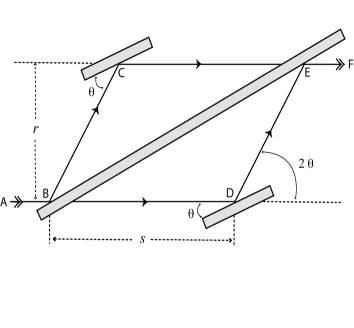
Figure 1: Schematic illustration of the COW neutron interferometer.

Let us now compute the phase $\varphi$ through the two trajectories of Fig. 1. First, we consider the trajectory BDE. Assuming that the segment BD is at $z=0$, we obtain

$$\varphi_{\sf BDE}=\frac{mg}{\hbar}\int_{\sf D}^{\sf E}z(t)\,dt.$$ (34)

For the trajectory BCE, we have

$$\varphi_{\sf BCE}=\frac{mg}{\hbar}\int_{\sf B}^{\sf C}z(t)\,dt+\frac{mgr}{\hbar}\int_{\sf C}^{\sf E}dt.$$ (35)

As the phase contribution along the segments DE and BC are equal, we get

$$\Delta\varphi\equiv\varphi_{\sf BCE}-\varphi_{\sf BDE}=\frac{mgr}{\hbar}\int_{\sf C}^{\sf E}dt.$$ (36)

Now, since the neutron velocity is constant along the segment CE, we have that

$$\int_{\sf C}^{\sf E}dt\equiv\frac{s}{v}=\frac{sm\lambda}{h},$$ (37)

where $s$ is the length of the segment CE, and $\lambda=h/(mv)$ is the de Broglie wavelength associated with the neutron. We thus obtain

$$\Delta\varphi=s\,\frac{2\pi gr\lambda m^{2}}{h^{2}},$$ (38)

which is exactly the gravitationally induced phase difference predicted for the COW experience [9]. It is important to remark that, in the above calculation, we have used the weak equivalence principle, according to which the gravitational ($m_{g}$) and the inertial ($m_{i}$) masses are assumed to be equal. If they were supposed to be different, the phase shift would be given by

$$\Delta\varphi=s\,\frac{2\pi gr\lambda m_{g}m_{i}}{h^{2}}.$$ (39)

6 Gravitational Aharonov-Bohm effect

As a second application we use the phase factor (30) to study the gravitational analog of the Aharonov-Bohm effect [13]. The usual (electromagnetic) Aharonov-Bohm effect consists in a shift, by a constant amount, of the electron interferometry wave pattern, in a region where there is no magnetic field, but there is a nontrivial gauge potential $A_{i}$. Analogously, the gravitational Aharonov-Bohm effect will consist in a similar shift of the same wave pattern, but produced by the presence of a gravitational gauge potential $B_{0i}$. Phenomenologically, this kind of effect might be present near a massive rapidly rotating source, like a neutron star, for example. Of course, differently from an ideal apparatus, in a real situation the gravitational field cannot be eliminated, and consequently the gravitational Aharonov-Bohm effect should be added to the other effects also causing a phase change.

Let us consider first the case in which there is no external field at all. If the electrons are emitted with a characteristic momentum $p$, then its wavefunction has the de Broglie wavelength $\lambda=h/p$. Denoting by $L$ the distance between slit and screen (see Fig. 2), and by $d$ the distance between the two holes, when the conditions $L\gg\lambda$, $L\gg x$ and $L\gg d$ are satisfied, the phase difference at a distance $x$ from the central point of the screen is given by

$$\delta^{0}\varphi(x)=\frac{2\pi xd}{L\lambda}.$$ (40)

This expression defines the wave pattern on the screen.

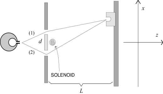
Figure 2: Schematic illustration of the Aharonov-Bohm electron interferometer.

We consider now the case in which a kind of infinite “gravitational solenoid” produces a purely static gravitomagnetic field flux concentrated in its interior. In the ideal situation, the gravitational field outside the solenoid vanishes completely, but there is a nontrivial gauge potential $B_{0i}$. When we let the electrons to move outside the solenoid, phase factors corresponding to paths lying on one side of the solenoid will interfere with phase factors corresponding to paths lying on the other side, which will produce an additional phase shift at the screen. Let us then calculate this additional phase shift. The gravitational phase factor (30) for the physical situation described above is

$$\Phi_{g}({\sf P}|{\sf Q})=\exp\left[-\frac{imc}{\hbar}\int_{\sf P}^{\sf Q}u^{0}\vec{B}_{0}\cdot d\vec{r}\right],$$ (41)

where $\vec{B}_{0}$ is the vector with components $B_{0}{}^{i}=-B_{0i}$. Since $u^{0}=\gamma\equiv[1-({v^{2}}/{c^{2}})]^{-1/2}$, and considering that the electron velocity $v$ is constant, we can write

$$\Phi_{g}({\sf P}|{\sf Q})=\exp\left[-\frac{i\gamma mc}{\hbar}\int_{\sf P}^{\sf Q}\vec{B}_{0}\cdot d\vec{r}\right].$$ (42)

Now, denoting by $\varphi_{1}$ the phase corresponding to a path lying on one side of the solenoid, and by $\varphi_{2}$ the phase corresponding to a path lying on the other side, the phase difference at the screen will be

$$\delta\varphi\equiv\varphi_{2}-\varphi_{1}=\frac{\gamma mc}{\hbar}\oint\vec{B}_{0}\cdot d\vec{r}=\frac{{\mathcal{E}}\,\Omega}{\hbar\,c},$$ (43)

where ${\mathcal{E}}=\gamma mc^{2}$ is the electron kinetic energy, and

$$\Omega=\oint\vec{B}_{0}\cdot d\vec{r}=\oint(\vec{\nabla}\times\vec{B}_{0})\cdot d\vec{\sigma}\equiv\oint\vec{H}\cdot d\vec{\sigma}$$ (44)

is the $\vec{H}$ flux inside the solenoid. In components, the gravitational field $\vec{H}$ is written as

$$H^{i}=\frac{1}{2}\epsilon^{ijk}\;(\partial_{j}B_{0k}-\partial_{k}B_{0j})=\frac{1}{2}\epsilon^{ijk}\;T_{0jk},$$ (45)

with $F_{0jk}$ the gravitational field strength defined in (2). Remembering that the axial torsion is defined by ${\mathcal{A}}^{\mu}=({1}/{6})\epsilon^{\mu\nu\rho\sigma}\,T_{\nu\rho\sigma}$, it is then an easy task to verify that $H^{i}={\mathcal{A}}^{i}$, with

$${\mathcal{A}}^{i}=-\frac{1}{2}\epsilon^{0ijk}\,T_{0jk}$$ (46)

the space components of the axial torsion. This shows that $H^{i}$ coincides with the axial torsion, which in turn represents the gravitomagnetic component of the gravitational field [14].

Expression (43) gives the phase difference produced by the interaction of the particle’s kinetic energy with a gauge potential, which gives rise to the gravitational Aharonov-Bohm effect. As this phase difference depends on the energy, it applies equally to massive and massless particles. It is worthy mentioning that, for the case of massive particles, if the inertial and gravitational masses were supposed to be different, the phase shift would assume the form

$$\delta\varphi=\frac{m_{g}}{m_{i}}\,\frac{{\mathcal{E}}\,\Omega}{\hbar\,c}.$$ (47)

It is also worthy mentioning that, whereas for massive particles it is a genuine quantum effect, for massless particles, due to the their intrinsic wave character, it can be considered as a classical effect. In fact, for ${\mathcal{E}}=h\omega$, Eq. (43) becomes

$$\delta\varphi=\frac{\omega\,\Omega}{c},$$ (48)

and we see that, in this case, the phase difference does not depend on the Planck’s constant.

In contrast with the electromagnetic Aharonov-Bohm effect, the phase difference in the gravitational case depends on the particle kinetic energy, which in turn depends on the particle’s mass and velocity. Like the electromagnetic case, however, the phase difference is independent of the position $x$ on the screen, and consequently the wave pattern defined by (40) will be whole shifted by a constant amount. It is also important to mention that the requirement of invariance of the gravitational phase factor under the translational gauge transformation (5) implies that

$$\Omega{\mathcal{E}}=nhc,$$ (49)

with $n$ an integer number. Differently from the electromagnetic case, where it is possible to define a quantum of magnetic flux, we see from the above equation that in the gravitational case it is not possible to define a particle-independent quantum of gravitomagnetic flux [15].

7 Quantum versus classical approaches

We proceed now to show that, in the classical limit, the nonintegrable phase factor approach reduces to the usual approach provided by the gravitational Lorentz force equation. In electromagnetism, the standard argument is well-known: the phase turning up in the quantum case is exactly the classical action, which leads to the Lorentz force. We intend, however, to illustrate the result directly, and for that we consider again the electron interferometry slit experiment, this time with a homogeneous static gravitomagnetic field $\vec{H}$ permeating the whole region between the slit and the screen (see Fig. 3). This field is supposed to point in the negative $y$-direction, and will produce a phase shift which is to be added to the phase (40) extant in the absence of gravitomagnetic field. This shift, according to Eq. (43), is given by ${\mathcal{E}}\Omega/\hbar c$, with $\Omega$ the flux through the surface $S$ circumscribed by the two trajectories.

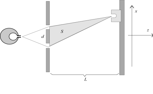
Figure 3: Schematic illustration of the electron interference experiment in a gravitomagnetic field. The only contribution to the phase-shift comes from the flux through the surface $S$ delimited by the two trajectories.

It is easily seen that $S=Ld/2$ for any value of $x$. The flux is consequently

$$\Omega=-H_{y}Ld/2,$$ (50)

where $\vec{H}=-H_{y}\,\hat{e}_{y}$, with $\hat{e}_{y}$ a unity vector in the $y$ direction. Therefore, the total phase difference will be

$$\delta\varphi=\frac{2\pi xd}{L\lambda}-\frac{{\mathcal{E}}H_{y}Ld}{2\hbar c}.$$ (51)

This is the result yielded by the phase-factor approach.

In the classical limit, the slit experiment can be interpreted in the following way. The electrons traveling through the gravitomagnetic field have their movement direction changed. This means that they experiment a force in the $x$-direction. For small $x$, we can approximately write the electrons velocity as $v\simeq v_{z}$. In this case, they will be transversally accelerated by the gravitomagnetic field during the time interval

$$\Delta t=\frac{L}{v_{z}}.$$ (52)

This transversal $x$-acceleration is given by

$$a_{x}=\frac{2x}{(\Delta t)^{2}}.$$ (53)

Since the attained acceleration is constant, we can choose a specific point to calculate it. Let us then consider the point of maximum intensity on the screen, which is determined by the condition $\delta\varphi=0$. This yields

$$x=\frac{H_{y}\,\lambda\,L^{2}\,{\mathcal{E}}}{2\,h\,c}.$$ (54)

The acceleration is then found to be

$$a_{x}=\,\frac{H_{y}\,\lambda\,{\mathcal{E}}\,v_{z}^{2}}{h\,c}.$$ (55)

From the classical point of view, therefore, we can say that the electrons experience a force in the $x$-direction given by

$${\mathcal{F}}_{x}\equiv\gamma\,m\,a_{x}=\frac{{\mathcal{E}}\,v_{z}\,H_{y}}{c}\,\frac{\lambda\,p}{h},$$ (56)

with $p=\gamma mv_{z}$ the electron momentum. Using now the de Broglie relation $\lambda=h/p$, it is possible to eliminate the Planck constant. We then get the classical result

$${\mathcal{F}}_{x}=\frac{\mathcal{E}}{c}\,v_{z}H_{y}=\frac{{\mathcal{E}}}{c}\;(\vec{v}\times\vec{H})_{x},$$ (57)

which gives rise to the equation of motion

$$\frac{Dp_{x}}{dt}=\frac{{\mathcal{E}}}{c}\;(\vec{v}\times\vec{H})_{x},$$ (58)

where $D/dt$ represents a time covariant derivative in the Weitzenböck connection. This is exactly the $x$-component of the gravitational Lorentz force equation (16) (see Appendix A). From this equation we see clearly that, when the inertial and gravitational masses coincide, the resulting trajectory does not depend on the mass of the particle, which is in accordance with the universality property of the gravitational interaction. It is important to remark that, even if the inertial and gravitational masses are not supposed to coincide, the teleparallel approach still yields a consistent description of the gravitational interaction [7]

8 Final remarks

Teleparallel gravity is a gauge theory for the translation group. Its fundamental field is, accordingly, a gauge potential $B^{a}{}_{\mu}$ with values in the Lie algebra of the translation group. In this formulation, gravitation becomes quite analogous to electromagnetism. Based on that analogy and relying on the phase-factor approach to Maxwell’s theory, a teleparallel nonintegrable phase-factor approach to gravitation has been developed, which represents the quantum mechanical version of the classical gravitational Lorentz force.

As a first application we have considered the COW experiment. By taking the Newtonian limit, we have shown that the formalism yields the correct quantum phase-shift induced on the neutrons by their interaction with Earth’s gravitational field. As this phase shift is produced by the coupling of the neutron mass with the component $B_{00}$ of the translational gauge potential, it can be considered as a gravitoelectric Aharonov-Bohm effect [16]. As a second application we have obtained the quantum phase-shift produced by the coupling of the particle’s kinetic energy with the components $B_{0i}$ of the gauge potential, which corresponds to the usual (gravitomagnetic) analog of the Aharonov-Bohm effect.

Finally, by considering a simple slit experiment in which the particles are allowed to pass through a region with a homogeneous gravitomagnetic field, we have shown that, in the classical limit, the (quantum) nonintegrable phase-factor approach coincides with the usual (classical) approach based on the gravitational Lorentz force equation. This means that, as far as only classical trajectories are concerned, both approaches give the same result. In addition, provided the gravitational and inertial masses are supposed to be equal, gravitation becomes universal in the classical limit in the sense that the resulting trajectories do not depend on the masses of the particles.

At the quantum level, however, there are deep conceptual changes with respect to classical gravity. The phase of the particle wavefunction acquires a fundamental status and depends on the particle mass (COW effect, obtained in the non-relativistic limit) or relativistic kinetic energy (gravitational Aharonov-Bohm effect). At the quantum level, therefore, gravitation is no more universal [17], although in the specific case of the non-relativistic COW experiment, by introducing a kind of quantum equivalence principle, it can be made independent of the mass when written in an appropriate way [18]. Concerning this point, it should be remarked that, since teleparallel gravity is able to describe gravitation independently of the validity or not of the equivalence principle [7], it will not require a quantum version of this principle to deal with gravitationally induced quantum effects. We can thus conclude that teleparallel gravity seems to provide a much more appropriate and consistent approach to study these effects.

Appendix A

Let us take the gravitational Lorentz force equation (16) written in the form

$$\frac{Du_{\mu}}{ds}\equiv\frac{du_{\mu}}{ds}-\Gamma^{\lambda}{}_{\mu\rho}\,u_{\lambda}\,u^{\rho}=T_{\lambda\mu\rho}\,u^{\lambda}\,u^{\rho}.$$ (59)

As already mentioned, it is equivalent to the geodesic equation of general relativity. Its left-hand side is the Weitzenböck covariant derivative of the four-velocity along the trajectory, and the right-hand side represents the gravitational force. In the specific case considered in section 7, where a gravitomagnetic field is present, only the components $T_{0ij}$ of torsion are nonvanishing. Consequently, the above force equation reduces to

$$\frac{Du_{i}}{ds}=T_{0ij}\,u^{0}\,u^{j}.$$ (60)

Using the relations $u^{0}=\gamma$ and $u^{j}=(\gamma v^{j})/c$, as well as the fact that the gravitomagnetic field does not change the absolute value of the particle velocity, and consequently $d\gamma/ds=0$, we obtain

$$\frac{Dv_{i}}{ds}=\gamma\,c\,T_{0ij}\,v^{j}.$$ (61)

Now, from Eq. (45) we see that $T_{0ij}=\epsilon_{ijk}\,H^{k}$. Therefore, by using that $ds=(c/\gamma)dt$, we get

$$\frac{Dv_{i}}{dt}=c\,\epsilon_{ijk}\,v^{j}\,H^{k}=c\,(\vec{v}\times\vec{H})_{i}.$$ (62)

The corresponding equation for the momentum components $p^{i}=\gamma mv^{i}$ is

$$\frac{Dp^{i}}{dt}=\frac{\mathcal{E}}{c}\,(\vec{v}\times\vec{H})^{i}.$$ (63)

The force appearing in the right-hand side is quite similar to the electromagnetic Lorentz force, with the kinetic energy replacing the electric charge, and the gravitomagnetic vector field $\vec{H}$ replacing the usual magnetic field.

References

References

- [1] Aharonov Y and Bohm D 1959 Phys. Rev. 115, 485
- [2] Wu, T T and Yang C N 1975 Phys. Rev. D12, 3845
- [3] The basic references on torsion gravity can be found in Hammond R T 2002 Rep. Prog. Phys. 65, 599
- [4] The name teleparallel gravity is normally used to denote the general three-parameter theory introduced in Hayashi K and Shirafuji T 1979 Phys. Rev. D19, 3524. Here, however, we use it as a synonymous for the teleparallel equivalent of general relativity.
- [5] For a recent appraisal on the general three-parameter teleparallel gravity, see Obukhov Yu N and Pereira J G 2003 Phys. Rev. D67, 044016
- [6] For a general description of the gauge approach to gravitation, see Hehl F W, McCrea J D, Mielke E W and Ne’emann Y 1995 Phys. Rep. 258, 1; see also Blagojević M 2002 Gravitation and Gauge Symmetries (Bristol: IOP Publishing).
- [7] Aldrovandi R, Pereira J G and Vu K H 2004, Gen. Relat. Grav. 36, 101 (gr-qc/0304106)
- [8] de Andrade V C and Pereira J G 1997 Phys. Rev. D56, 4689
- [9] Overhauser A W and Colella R 1974 Phys. Rev. Lett. 33, 1237; Colella R, Overhauser A W and Werner S A Phys. Rev. Lett. 34, 1472
- [10] Aldrovandi R and Pereira J G 1995 An Introduction to Geometrical Physics (Singapore: World Scientific).
- [11] de Andrade V C, Guillen L C T and Pereira J G 2000 Phys. Rev. Lett. 84, 4533
- [12] de Andrade V C, Guillen L C T and Pereira J G 2001 Phys. Rev. D64, 027502
- [13] See, for example, Lawrence A K, Leiter D and Samozi G 1973 Nuovo Cimento 17B, 113; Ford L H and Vilenkin A 1981 J. Phys. A14, 2353; Bezerra V B 1989 J. Math. Phys. 30, 2895; Bezerra V B 1991 Class. Quantum Grav. 8, 1939
- [14] Pereira J G, Vargas T and Zhang C M 2001 Class. Quant. Grav. 18, 833
- [15] Harris E G 1996 Am. J. Phys. 64, 378
- [16] The same notation is used in the electromagnetic case. See, for example, Peshkin M and Tonomura A 1989 The Aharonov-Bohm Effect (Berlin: Springer-Verlag), Lecture Notes in Physics 340
- [17] Greenberger D 1968 Ann. Phys. 47, 116; Greenberger D and Overhauser A W 1979 Rev. Mod. Phys. 51, 43
- [18] Lämmerzahl C 1996 Gen. Rel. Grav. 28, 1043; Lämmerzahl C 1998 Acta Phys. Pol. 29, 1057