Gravitational and electromagnetic fields near an anti-de Sitter-like infinity

Abstract

We analyze asymptotic structure of general gravitational and electromagnetic fields near an anti-de Sitter-like conformal infinity. Dependence of the radiative component of the fields on a null direction along which the infinity is approached is obtained. The directional pattern of outgoing and ingoing radiation, which supplements standard peeling property, is determined by the algebraic (Petrov) type of the fields and also by orientation of principal null directions with respect to the timelike infinity. The dependence on the orientation is a new feature if compared to spacelike infinity.

In spacetimes which are asymptotically flat the behavior of radiative gravitational and electromagnetic fields near infinity has been rigorously analyzed by means of now classical techniques Bondi et al. (1962); Penrose (1965); Penrose and Rindler (1986). However, it still remains an open problem to fully characterize the asymptotic properties of more general exact solutions of the Einstein-Maxwell equations. Even in spacetimes which admit a smooth infinity ${\mathcal{I}}$ the concept of radiation is not obvious when the cosmological constant $\Lambda$ is nonvanishing. If we define radiative component of field as the $\eta^{-1}$ term of the field with respect to a parallelly transported tetrad along a null geodesic ($\eta$ being affine parameter) then for ${\Lambda\neq 0}$ the radiation depends on the direction along which geodesics approach a given point at ${\mathcal{I}}$ Penrose (1965); Penrose and Rindler (1986).

It is natural to analyze and describe such dependence. Recently, we studied Krtouš et al. (2003) this behavior of fields near ${\mathcal{I}}$ in the case $\Lambda>0$ and demonstrated that the directional pattern of radiation close to de Sitter-like infinity has a universal character that is determined by the algebraic type of the fields. In the present work we investigate the complementary situation when $\Lambda<0$. Interestingly, although the method is similar to the previous case, the results turn out to be more complicated, and completely new phenomena occur. This stems from the fundamental difference that the anti-de Sitter-like infinity ${\mathcal{I}}$ is timelike, and thus admits a “richer structure” of radiative patterns. This fact was recently demonstrated by analyzing radiation generated by accelerating black holes in an anti-de Sitter universe Podolský et al. (2003): ${\mathcal{I}}$ is divided by the Killing horizons into several domains with a different structure of principal null directions, in which the patterns of radiation differ. Moreover, ingoing and outgoing radiation have to be treated separately. It is the purpose of our work to generalize these results and to describe all the possible radiative patterns for gravitational and electromagnetic fields near an anti-de Sitter-like infinity.

A study of spacetimes with ${\Lambda\not=0}$ is motivated also by the fact that they have now become commonly used in various branches of physical research, e.g. in inflationary models, brane cosmologies, supergravity or string theories, in particular due to the AdS/CFT correspondence.

I Spacetime infinity, fields and tetrads

The conformal infinity ${\mathcal{I}}$ can be introduced Penrose (1965); Penrose and Rindler (1986) as a boundary of physical spacetime ${\mathcal{M}}$ with physical metric ${\boldsymbol{g}}$, when embedded into a larger conformal manifold ${\tilde{\mathcal{M}}}$ with conformal metric ${{\tilde{{\boldsymbol{g}}}}=\omega^{2}{\boldsymbol{g}}}$; the conformal factor $\omega$ (negative in ${\mathcal{M}}$) vanishes on ${\mathcal{I}}$. Assuming ${\tilde{{\boldsymbol{g}}}}$ is regular there, the metric ${\boldsymbol{g}}$ is “infinite” on ${\mathcal{I}}$, and ${\mathcal{I}}$ is thus infinitely distant from the interior of spacetime ${\mathcal{M}}$. We will be interested here in timelike conformal infinity which is characterized by a spacelike gradient $\mathbf{d}\omega$ on ${\mathcal{I}}$. The conformal metric ${\tilde{{\boldsymbol{g}}}}$ near such an anti-de Sitter-like infinity can always be decomposed into Lorentzian 3-metric ${{}^{\mathcal{I}}{\tilde{{\boldsymbol{g}}}}}$ tangent to ${\mathcal{I}}$, and a part orthogonal to it,

$${\boldsymbol{g}}=\omega^{-2}({{}^{\mathcal{I}}{\tilde{{\boldsymbol{g}}}}}+{\tilde{N}}^{2}\,\mathbf{d}\omega{}^{2}){\mbox{\;.}}$$ (1)

Spacelike unit vector ${{\boldsymbol{\mathbf{n}}}}$ normal to the infinity is then

$${{\boldsymbol{\mathbf{n}}}}^{\mu}=-\omega^{-1}{\tilde{N}}\,{\boldsymbol{g}}^{\mu\nu}\,\mathbf{d}_{\nu}\omega{\mbox{\;.}}$$ (2)

We denote the vectors of an orthonormal tetrad as ${{{\boldsymbol{\mathbf{t}}}},\,{{\boldsymbol{\mathbf{q}}}},\,{{\boldsymbol{\mathbf{r}}}},\,{{\boldsymbol{\mathbf{s}}}}}$ (${{\boldsymbol{\mathbf{t}}}}$ timelike) and the associated null tetrad as

$${{\boldsymbol{\mathbf{k}}}} =\textstyle{\frac{1}{\sqrt{2}}}({{\boldsymbol{\mathbf{t}}}}+{{\boldsymbol{\mathbf{q}}}}){\mbox{\;,\quad}} {{\boldsymbol{\mathbf{l}}}} =\textstyle{\frac{1}{\sqrt{2}}}({{\boldsymbol{\mathbf{t}}}}-{{\boldsymbol{\mathbf{q}}}}){\mbox{\;,}}$$ (3)

$${{\boldsymbol{\mathbf{m}}}} =\textstyle{\frac{1}{\sqrt{2}}}({{\boldsymbol{\mathbf{r}}}}-i\,{{\boldsymbol{\mathbf{s}}}}){\mbox{\;,\quad}} {\bar{{\boldsymbol{\mathbf{m}}}}} =\textstyle{\frac{1}{\sqrt{2}}}({{\boldsymbol{\mathbf{r}}}}+i\,{{\boldsymbol{\mathbf{s}}}}){\mbox{\;,}}$$

so that ${{\boldsymbol{\mathbf{k}}}}\mathbin{\boldsymbol{\cdot}}{{\boldsymbol{\mathbf{l}}}}\!=\!-1$, ${{\boldsymbol{\mathbf{m}}}}\mathbin{\boldsymbol{\cdot}}{\bar{{\boldsymbol{\mathbf{m}}}}}\!=\!1$. In the null tetrad the Weyl tensor ${\boldsymbol{\mathbf{C}}}_{\alpha\beta\gamma\delta}$ can be parameterized by five complex coefficients $\Psi_{j}$,  ${j\!=\!0,\,1,\,2,\,3,\,4}$, and the electromagnetic tensor ${\boldsymbol{\mathbf{F}}}_{\alpha\beta}$ by three coefficients $\Phi_{j}$,  ${j\!=\!0,\,1,\,2}$, see Kramer et al. (1980); Krtouš and Podolský (2003).

We wish to investigate behavior of these field components in an appropriate interpretation tetrad parallelly transported along future oriented null geodesics $z(\eta)$ which reach a given point ${P_{\scriptscriptstyle{\infty}}}$ at ${\mathcal{I}}$. Such geodesics form two distinct families which are distinguished by their orientation $\epsilon$: geodesics outgoing to ${\mathcal{I}}$ which end at ${P_{\scriptscriptstyle{\infty}}}$ (${\epsilon=+1}$), and geodesics ingoing from ${\mathcal{I}}$ which start at ${P_{\scriptscriptstyle{\infty}}}$ (${\epsilon=-1}$). A geodesic thus reaches the point ${P_{\scriptscriptstyle{\infty}}}$ for the affine parameter ${\eta\to\epsilon\,\infty}$. The lapse-like function ${{\tilde{N}}>0}$ and the conformal factor $\omega<0$ can be expanded along the geodesic in powers of ${1/\eta}$ as ${{\tilde{N}}\approx{\tilde{N}}_{\scriptscriptstyle{\infty}}+\dots}$, ${\omega\approx\epsilon\,\omega_{*}\eta^{-1}+\dots}$. Here, ${{\tilde{N}}_{\scriptscriptstyle{\infty}}\!=\!{\tilde{N}}|_{{P_{\scriptscriptstyle{\infty}}}}}$ is the same for all geodesics reaching ${P_{\scriptscriptstyle{\infty}}}$. Moreover, we require that the approach of all geodesics to the infinity is “comparable”, independent on their direction, so we assume $\omega_{*}$ to be a (negative) constant. It is equivalent to fixing the momentum ${p_{\mathrm{o}}={\boldsymbol{\mathbf{p}}}\mathbin{\boldsymbol{\cdot}}{{\boldsymbol{\mathbf{n}}}}}$ (${{\boldsymbol{\mathbf{p}}}=\frac{Dz}{d\eta}}$ being 4-momentum) at a given small value of $\omega$. This choice of the “comparable” approach to ${\mathcal{I}}$ is the only one we can apply unless there are additional geometrical structures (as, e.g., a Killing vector) which would allow us to fix a different quantity (e.g., the energy). We will see that this choice has significant consequences for the character of the radiation pattern.

The interpretation tetrad ${{{\boldsymbol{\mathbf{k}}}}_{\mathrm{i}},\,{{\boldsymbol{\mathbf{l}}}}_{\mathrm{i}},{{\boldsymbol{\mathbf{m}}}}_{\mathrm{i}},\,{\bar{{\boldsymbol{\mathbf{m}}}}}_{\mathrm{i}}}$ also has to be specified “comparably” for all geodesics having different directions. We require that: (i) Null vector ${{\boldsymbol{\mathbf{k}}}}_{\mathrm{i}}$ is proportional to the tangent vector of the geodesic

$${{\boldsymbol{\mathbf{k}}}}_{\mathrm{i}}=\frac{1}{\sqrt{2}{\tilde{N}}_{\scriptscriptstyle{\infty}}}\,\frac{Dz}{d\eta}{\mbox{\;,}}$$ (4)

the factor being independent of the direction. (ii) Null vector ${{\boldsymbol{\mathbf{l}}}}_{\mathrm{i}}$ is fixed by normalization ${{{\boldsymbol{\mathbf{k}}}}_{\mathrm{i}}\mathbin{\boldsymbol{\cdot}}{{\boldsymbol{\mathbf{l}}}}_{\mathrm{i}}=-1}$ and requirement that normal vector ${{\boldsymbol{\mathbf{n}}}}$ belongs to ${{\boldsymbol{\mathbf{k}}}}_{\mathrm{i}}{\text{-}}{{\boldsymbol{\mathbf{l}}}}_{\mathrm{i}}$ plane Penrose and Rindler (1986). Remaining vectors ${{{\boldsymbol{\mathbf{m}}}}_{\mathrm{i}},\,{\bar{{\boldsymbol{\mathbf{m}}}}}_{\mathrm{i}}}$ cannot be specified canonically. Below, these vectors will be chosen arbitrarily and we will only study moduli $\left\lvert\Psi^{{\mathrm{i}}}_{4}\right\rvert$ and $\left\lvert\Phi^{{\mathrm{i}}}_{2}\right\rvert$ of the radiative field components which are independent of such a choice.

As ${\eta\to\epsilon\,\infty}$, the interpretation tetrad is “infinitely” boosted with respect to an observer with 4-velocity tangent to ${\mathcal{I}}$. To see this explicitly, we introduce an auxiliary tetrad ${{{\boldsymbol{\mathbf{t}}}}_{\mathrm{b}},\,{{\boldsymbol{\mathbf{q}}}}_{\mathrm{b}},\,{{\boldsymbol{\mathbf{r}}}}_{\mathrm{b}},\,{{\boldsymbol{\mathbf{s}}}}_{\mathrm{b}}}$ adapted to the infinity, ${{{\boldsymbol{\mathbf{q}}}}_{\mathrm{b}}=\epsilon\,{{\boldsymbol{\mathbf{n}}}}}$, with timelike vector ${{\boldsymbol{\mathbf{t}}}}_{\mathrm{b}}$ given by the projection of ${{\boldsymbol{\mathbf{k}}}}_{\mathrm{i}}$ to ${\mathcal{I}}$,

$${{\boldsymbol{\mathbf{t}}}}_{\mathrm{b}}\propto{{\boldsymbol{\mathbf{k}}}}_{\mathrm{i}}-({{\boldsymbol{\mathbf{k}}}}_{\mathrm{i}}\mathbin{\boldsymbol{\cdot}}{{\boldsymbol{\mathbf{n}}}})\,{{\boldsymbol{\mathbf{n}}}}{\mbox{\;,}}$$ (5)

and the spatial vectors ${{{\boldsymbol{\mathbf{r}}}}_{\mathrm{b}},\,{{\boldsymbol{\mathbf{s}}}}_{\mathrm{b}}}$ being identical to ${{{\boldsymbol{\mathbf{r}}}}_{\mathrm{i}},\,{{\boldsymbol{\mathbf{s}}}}_{\mathrm{i}}}$. Checking that ${{{\boldsymbol{\mathbf{k}}}}_{\mathrm{i}}\mathbin{\boldsymbol{\cdot}}{{\boldsymbol{\mathbf{n}}}}\approx{\textstyle\epsilon\frac{1}{\sqrt{2}}}\,\eta^{-1}}$ we obtain

$$\begin{gathered}{{\boldsymbol{\mathbf{k}}}}_{\mathrm{i}}=B_{\mathrm{i}}\;{{\boldsymbol{\mathbf{k}}}}_{\mathrm{b}}=\eta^{-1}{\textstyle\frac{1}{\sqrt{2}}}\,({{\boldsymbol{\mathbf{t}}}}_{\mathrm{b}}+\epsilon\,{{\boldsymbol{\mathbf{n}}}}){\mbox{\;,\quad}}{{\boldsymbol{\mathbf{m}}}}_{\mathrm{i}}={{\boldsymbol{\mathbf{m}}}}_{\mathrm{b}}{\mbox{\;,}}\\ {{\boldsymbol{\mathbf{l}}}}_{\mathrm{i}}=B_{\mathrm{i}}^{-1}\,{{\boldsymbol{\mathbf{l}}}}_{\mathrm{b}}=\;\;\eta\;{\textstyle\frac{1}{\sqrt{2}}}\,({{\boldsymbol{\mathbf{t}}}}_{\mathrm{b}}-\epsilon\,{{\boldsymbol{\mathbf{n}}}}){\mbox{\;,\quad}}{\bar{{\boldsymbol{\mathbf{m}}}}}_{\mathrm{i}}={\bar{{\boldsymbol{\mathbf{m}}}}}_{\mathrm{b}}{\mbox{\;,}}\end{gathered}$$ (6)

${B_{\mathrm{i}}=1/\eta}$ being a boost parameter which approaches zero on ${\mathcal{I}}$, i.e., it represents an “infinite” boost. Under this the fields transform as ${\Psi^{{\mathrm{i}}}_{j}=B_{\mathrm{i}}^{2-j}\,\Psi^{{\mathrm{b}}}_{j}}$, ${\Phi^{{\mathrm{i}}}_{j}=B_{\mathrm{i}}^{1-j}\,\Phi^{{\mathrm{b}}}_{j}}$. Considering the behavior (10) in a tetrad adapted to ${\mathcal{I}}$ we obtain peeling-off property.

II Directional pattern of radiation

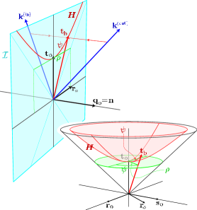
Figure 1: Parametrization of a null direction ${{\boldsymbol{\mathbf{k}}}}$ near timelike infinity ${\mathcal{I}}$. All null directions form three families: outgoing directions (${{{\boldsymbol{\mathbf{k}}}}\mathbin{\boldsymbol{\cdot}}{{\boldsymbol{\mathbf{n}}}}>0}$, vector ${{\boldsymbol{\mathbf{k}}}}^{(\mathrm{out})}$ in the figure), ingoing directions (${{{\boldsymbol{\mathbf{k}}}}\mathbin{\boldsymbol{\cdot}}{{\boldsymbol{\mathbf{n}}}}<0}$, vector ${{\boldsymbol{\mathbf{k}}}}^{(\mathrm{in})}$), and directions tangent to ${\mathcal{I}}$. With respect to a reference tetrad ${{{\boldsymbol{\mathbf{t}}}}_{\mathrm{o}},\,{{\boldsymbol{\mathbf{q}}}}_{\mathrm{o}},\,{{\boldsymbol{\mathbf{r}}}}_{\mathrm{o}},\,{{\boldsymbol{\mathbf{s}}}}_{\mathrm{o}}}$, a direction ${{\boldsymbol{\mathbf{k}}}}$ can be parameterized by boost $\psi$, angle $\phi$ and orientation $\epsilon$, or by parameters $\rho$, $\phi$, or by a complex number $R$. In the upper diagram, the vectors ${{{\boldsymbol{\mathbf{t}}}}_{\mathrm{o}},\,{{\boldsymbol{\mathbf{q}}}}_{\mathrm{o}},\,{{\boldsymbol{\mathbf{r}}}}_{\phi}}$ are depicted, remaining spatial direction ${{\boldsymbol{\mathbf{s}}}}_{\phi}$ is suppressed; in the bottom the direction ${{{\boldsymbol{\mathbf{q}}}}_{\mathrm{o}}\!=\!{{\boldsymbol{\mathbf{n}}}}}$ is omitted. The parameters ${\psi,\,\phi}$ specify the normalized orthogonal projection ${{\boldsymbol{\mathbf{t}}}}_{\mathrm{b}}$ of ${{\boldsymbol{\mathbf{k}}}}$ into ${\mathcal{I}}$, cf. Eqs. (5), (7). To parametrize ${{\boldsymbol{\mathbf{k}}}}$ uniquely, we have to specify also its orientation ${\epsilon=\operatorname{sign}({{\boldsymbol{\mathbf{k}}}}\!\mathbin{\boldsymbol{\cdot}}\!{{\boldsymbol{\mathbf{n}}}})}$ with respect to ${\mathcal{I}}$. Vectors ${{\boldsymbol{\mathbf{t}}}}_{\mathrm{b}}$ corresponding to all outgoing (or ingoing) null directions form a hyperbolic surface $\boldsymbol{H}$. This can be radially mapped onto a two-dimensional disk tangent to the hyperboloid at ${{\boldsymbol{\mathbf{t}}}}_{\mathrm{o}}$, which can be parametrized by angle $\phi$ and radial coordinate ${\rho=\tanh\psi}$. In the exceptional case ${\epsilon=0}$ the boost ${\psi\!\to\!\infty}$, and ${{{\boldsymbol{\mathbf{k}}}}\propto{{\boldsymbol{\mathbf{t}}}}_{\mathrm{b}}\!+\!{{\boldsymbol{\mathbf{r}}}}_{\phi}}$ is tangent to ${\mathcal{I}}$. Finally, parameter $R$ is the Lorentzian stereographic representation of ${\psi,\,\phi,\,\epsilon}$, cf. Eq. (8).

Now we explicitly derive dependence of the radiation on the direction of a null geodesic along which the infinity is approached. First, we parametrize this direction with respect to a suitable reference tetrad ${{{\boldsymbol{\mathbf{t}}}}_{\mathrm{o}},\,{{\boldsymbol{\mathbf{q}}}}_{\mathrm{o}},\,{{\boldsymbol{\mathbf{r}}}}_{\mathrm{o}},\,{{\boldsymbol{\mathbf{s}}}}_{\mathrm{o}}}$ adapted to the conformal infinity, namely ${{{\boldsymbol{\mathbf{q}}}}_{\mathrm{o}}={{\boldsymbol{\mathbf{n}}}}}$. The vectors ${{\boldsymbol{\mathbf{t}}}}_{\mathrm{o}},\,{{\boldsymbol{\mathbf{r}}}}_{\mathrm{o}},\,{{\boldsymbol{\mathbf{s}}}}_{\mathrm{o}}$ can be fixed conveniently with help of the particular geometry of the spacetime. The timelike vector ${{\boldsymbol{\mathbf{t}}}}_{\mathrm{b}}$ is related to the vector ${{\boldsymbol{\mathbf{t}}}}_{\mathrm{o}}$ by a boost (cf. Fig. 1)

$${{\boldsymbol{\mathbf{t}}}}_{\mathrm{b}}=\cosh\psi\;{{\boldsymbol{\mathbf{t}}}}_{\mathrm{o}}+\sinh\psi\;{{\boldsymbol{\mathbf{r}}}}_{\phi}{\mbox{\;,}}$$ (7)

with ${{\boldsymbol{\mathbf{r}}}}_{\phi}\!=\!\cos\phi\;{{\boldsymbol{\mathbf{r}}}}_{\mathrm{o}}\!+\sin\phi\;{{\boldsymbol{\mathbf{s}}}}_{\mathrm{o}}$ (and ${{\boldsymbol{\mathbf{s}}}}_{\phi}\!=\!-\!\sin\phi\;{{\boldsymbol{\mathbf{r}}}}_{\mathrm{o}}\!+\cos\phi\;{{\boldsymbol{\mathbf{s}}}}_{\mathrm{o}}$). Because the vector ${{\boldsymbol{\mathbf{t}}}}_{\mathrm{b}}$ is related to the projection of ${{\boldsymbol{\mathbf{k}}}}_{\mathrm{i}}$ we can use the “Lorentzian angles” $\psi$, $\phi$ and the orientation $\epsilon$ to parameterize the direction of the null geodesic. Instead of these parameters it is also convenient to use their Lorentzian stereographic representation $R$,

$$R=\begin{cases}\tanh(\psi/2)\,\exp(-i\phi)&\;\text{for $\epsilon=+1$}{\mbox{\;,}}\\[1.29167pt] \coth(\psi/2)\,\exp(-i\phi)&\;\text{for $\epsilon=-1$}{\mbox{\;.}}\end{cases}$$ (8)

We allow also the infinite value ${R=\infty}$ corresponding to ${\psi=0}$, ${\epsilon=-1}$, i.e., ${{{\boldsymbol{\mathbf{k}}}}\propto\frac{1}{\sqrt{2}}({{\boldsymbol{\mathbf{t}}}}_{\mathrm{o}}-{{\boldsymbol{\mathbf{q}}}}_{\mathrm{o}})}$.

Next, we express the field components $\Psi^{{\mathrm{o}}}_{j}$ (and $\Phi^{{\mathrm{o}}}_{j}$) with respect to the reference tetrad using algebraically privileged principal null directions (PNDs). PNDs of gravitational (or electromagnetic, respectively) field are null directions ${{\boldsymbol{\mathbf{k}}}}$ such that ${\Psi_{0}=0}$ (or ${\Phi_{0}=0}$) in a null tetrad ${{{\boldsymbol{\mathbf{k}}}},\,{{\boldsymbol{\mathbf{l}}}},\,{{\boldsymbol{\mathbf{m}}}},\,{\bar{{\boldsymbol{\mathbf{m}}}}}}$ (a choice of ${{{\boldsymbol{\mathbf{l}}}},\,{{\boldsymbol{\mathbf{m}}}},\,{\bar{{\boldsymbol{\mathbf{m}}}}}}$ being irrelevant). If we parametrize ${{\boldsymbol{\mathbf{k}}}}$ by the above stereographic parameter $R$, the condition on PND with respect to the reference tetrad takes the form Kramer et al. (1980); Krtouš and Podolský (2003)

$$\begin{gathered}R^{4}\Psi^{{\mathrm{o}}}_{4}+4R^{3}\Psi^{{\mathrm{o}}}_{3}+6R^{2}\Psi^{{\mathrm{o}}}_{2}+4R\,\Psi^{{\mathrm{o}}}_{1}+\Psi^{{\mathrm{o}}}_{0}=0{\mbox{\;,}}\\ R^{2}\Phi^{{\mathrm{o}}}_{2}+2R\,\Phi^{{\mathrm{o}}}_{1}+\Phi^{{\mathrm{o}}}_{0}=0{\mbox{\;,\quad}}\text{respectively}{\mbox{\;.}}\end{gathered}$$ (9)

There are thus four (or two) PNDs characterized by the roots ${R=R_{n}}$, ${n=1,\,2,\,3,\,4}$ (or ${R=R^{\scriptscriptstyle\mathrm{EM}}_{n}}$, ${n=1,\,2}$). In a generic situation we have ${\Psi^{{\mathrm{o}}}_{4}\neq 0}$, and the remaining components $\Psi^{{\mathrm{o}}}_{j}$,  ${j=0,\,1,\,2,\,3}$, can be expressed in terms of $R_{n}$ (analogously for $\Phi^{{\mathrm{o}}}_{j}$,  ${j=0,\,1}$), see Krtouš et al. (2003).

Using the conditions (i), (ii) above and Eqs. (6), (7), (8), we can now find the Lorentz transformation from the reference tetrad to the interpretation tetrad (up to a non-unique rotation in the ${{{\boldsymbol{\mathbf{m}}}}_{\mathrm{i}}{\text{-}}{\bar{{\boldsymbol{\mathbf{m}}}}}_{\mathrm{i}}}$ plane). We can thus express the field components $\Psi^{{\mathrm{i}}}_{4}$ (or $\Phi^{{\mathrm{i}}}_{2}$) with respect to the interpretation tetrad in terms of $\Psi^{{\mathrm{o}}}_{j}$ (or $\Phi^{{\mathrm{o}}}_{j}$), and consequently in terms of the parameters $R_{n}$ of PNDs and $\Psi^{{\mathrm{o}}}_{4}$ (or ${R^{\scriptscriptstyle\mathrm{EM}}_{n}}$ and $\Phi^{{\mathrm{o}}}_{2}$), cf. Krtouš et al. (2003). Taking into account a typical behavior of the fields in a tetrad adapted to ${\mathcal{I}}$ (e.g., Penrose and Rindler (1986)),

$$\Psi^{{\mathrm{o}}}_{n}\approx\Psi^{{\mathrm{o}}}_{n}{}_{*}\;\eta^{-3}{\mbox{\;,\quad}}\Phi^{{\mathrm{o}}}_{n}\approx\Phi^{{\mathrm{o}}}_{n}{}_{*}\;\eta^{-2}{\mbox{\;,}}$$ (10)

we finally obtain the directional pattern of radiation—the dependence of radiative components of gravitational and electromagnetic fields on the null direction (given by $R$) along which the timelike infinity is approached:

$$\begin{split}\left\lvert\Psi^{{\mathrm{i}}}_{4}\right\rvert&\approx\left\lvert\Psi^{{\mathrm{o}}}_{4}{}_{*}\right\rvert\,\eta^{-1}\,\bigl{\lvert}1-\left\lvert R\right\rvert^{2}\bigr{\rvert}^{-2}\\ &\quad\quad\times{\textstyle\left\lvert 1-\frac{R_{1}}{R_{\mathrm{m}}}\right\rvert\left\lvert 1-\frac{R_{2}}{R_{\mathrm{m}}}\right\rvert\left\lvert 1-\frac{R_{3}}{R_{\mathrm{m}}}\right\rvert\left\lvert 1-\frac{R_{4}}{R_{\mathrm{m}}}\right\rvert}{\mbox{\;,}}\end{split}$$ (11)

$$\begin{split}\left\lvert\Phi^{{\mathrm{i}}}_{2}\right\rvert&\approx\left\lvert\Phi^{{\mathrm{o}}}_{2}{}_{*}\right\rvert\eta^{-1}\bigl{\lvert}1-\left\lvert R\right\rvert^{2}\bigr{\rvert}^{-1}{\textstyle\left\lvert 1-\frac{R^{\scriptscriptstyle\mathrm{EM}}_{1}}{R_{\mathrm{m}}}\right\rvert\!\left\lvert 1-\frac{R^{\scriptscriptstyle\mathrm{EM}}_{2}}{R_{\mathrm{m}}}\right\rvert}{\mbox{\;.}}\end{split}$$ (12)

Here, the complex number $R_{\mathrm{m}}$,

$$R_{\mathrm{m}}={\bar{R}}^{-1}=\coth^{\epsilon}(\psi/2)\,\exp(-i\phi){\mbox{\;,}}$$ (13)

characterizes a direction obtained from the direction $R$ by a reflection with respect to ${\mathcal{I}}$, i.e., the mirrored direction with ${\psi_{\mathrm{m}}=\psi}$, ${\phi_{\mathrm{m}}=\phi}$ but opposite orientation ${\epsilon_{\mathrm{m}}=-\epsilon}$.

The expression (11) has been derived assuming ${\Psi^{{\mathrm{o}}}_{4}\neq 0}$, i.e., ${R_{n}\neq\infty}$. However, to describe PND oriented along ${{\boldsymbol{\mathbf{l}}}}_{\mathrm{o}}$ it is necessary to use a different component $\Psi^{{\mathrm{o}}}_{j}$ as a normalization factor. E.g., with $\Psi^{{\mathrm{o}}}_{0}$ we obtain

$$\begin{split}\left\lvert\Psi^{{\mathrm{i}}}_{4}\right\rvert&\approx\left\lvert\Psi^{{\mathrm{o}}}_{0}{}_{*}\right\rvert\,\eta^{-1}\,\bigl{\lvert}1-\left\lvert R_{\mathrm{m}}\right\rvert^{2}\bigr{\rvert}^{-2}\\ &\quad\quad\times{\textstyle\bigl{\lvert}1\!-\!\frac{R_{1}{}_{\mathrm{m}}}{R}\bigr{\rvert}\bigl{\lvert}1\!-\!\frac{R_{2}{}_{\mathrm{m}}}{R}\bigr{\rvert}\bigl{\lvert}1\!-\!\frac{R_{3}{}_{\mathrm{m}}}{R}\bigr{\rvert}\bigl{\lvert}1\!-\!\frac{R_{4}{}_{\mathrm{m}}}{R}\bigr{\rvert}}{\mbox{\;.}}\end{split}$$ (14)

Interestingly, the radiation pattern thus has the same form if we reflect all PNDs, ${R_{n}\to(R_{n})_{\mathrm{m}}}$, and switch ingoing and outgoing directions, ${R\to R_{\mathrm{m}}}$.

III Discussion

The expressions (11) and (12) characterize the asymptotic behavior of the fields near anti-de Sitter-like infinity. We will analyze here only gravitational field, discussion of electromagnetic one is analogous. First, we observe that the radiation “blows up” for directions with ${\left\lvert R\right\rvert\!=\!1}$ (i.e., ${\psi\to\infty}$). These are null directions tangent to the infinity ${\mathcal{I}}$, and thus they do not represent a direction of any geodesic approaching the infinity from the “interior” of the spacetime. The reason for this divergent behavior is purely kinematic: when we required the “comparable” approach of geodesics to the infinity we had fixed the component of the 4-momentum ${{\boldsymbol{\mathbf{p}}}}\propto{{\boldsymbol{\mathbf{k}}}}_{\mathrm{i}}$ normal to ${\mathcal{I}}$. Clearly, such a condition implies an “infinite” rescaling if ${{\boldsymbol{\mathbf{k}}}}_{\mathrm{i}}$ is tangent to ${\mathcal{I}}$ which results in the divergence of $\left\lvert\Psi^{{\mathrm{i}}}_{4}\right\rvert$.

The divergence at ${\left\lvert R\right\rvert\!=\!1}$ splits the radiation pattern into two components—the pattern for outgoing geodesics (${\left\lvert R\right\rvert\!<\!1}$, ${\epsilon=+1}$) and that for ingoing geodesics (${\left\lvert R\right\rvert\!>\!1}$, ${\epsilon=-1}$). These two different patterns are depicted in diagrams in Fig. 2 separately.

From Eq. (11) it is obvious that there are, in general, four directions along which the radiation vanishes, namely PNDs reflected with respect to ${\mathcal{I}}$, given by ${R\!=\!(R_{n})_{\mathrm{m}}}$. Outgoing PNDs give rise to zeros in the radiation pattern for ingoing geodesics, and vice versa. A qualitative shape of the radiation pattern thus depends on (i) orientation of PNDs with respect to ${\mathcal{I}}$ (i.e., the number of outgoing/ingoing/tangent PNDs), and (ii) degeneracy of PNDs (Petrov type of the spacetime). Depending on these factors there are 51 qualitatively different shapes of the radiation patterns (3 for Petrov type N spacetimes, 9 for type III, 6 for D, 18 for II, and 15 for type I spacetimes); 21 pairs of them are related by the duality of Eqs. (11) and (14). The most typical are shown in Fig. 2.

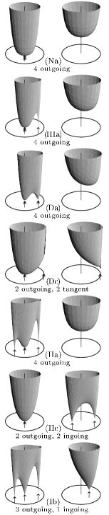
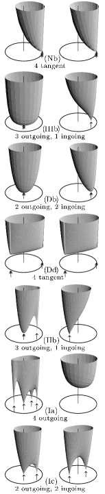
Figure 2: Directional patterns of radiation near a timelike ${\mathcal{I}}$. All 11 qualitatively different shapes of the pattern when PNDs are not tangent to ${\mathcal{I}}$ are shown (remaining 9 are related by a simple reflection with respect to ${\mathcal{I}}$). Patterns (Nb), (Dc), (Dd) are just few examples with PNDs tangent to ${\mathcal{I}}$. Each diagram consists of patterns for ingoing (left) and outgoing geodesics (right). $\left\lvert\Psi^{{\mathrm{i}}}_{4}\right\rvert$ is drawn on the vertical axis, directions of geodesics are represented on the horizontal disc by coordinates ${\rho,\,\phi}$ introduced in Fig. 1. Reflected [degenerated] PNDs are indicated by [multiple] arrows under the discs. For PNDs that are not tangent to ${\mathcal{I}}$ these are directions of vanishing radiation. The Petrov type (N, III, D, II, I) corresponding to the degeneracy of PNDs is indicated by labels of diagrams, number of ingoing and outgoing PNDs is also displayed.

The reference tetrad can be chosen to capture a geometry of the spacetime. To simplify the radiation pattern we can also adapt it to the algebraic structure, i.e., to correlate the tetrad with PNDs. For example, we can always orient ${{\boldsymbol{\mathbf{t}}}}_{\mathrm{o}}$ along the orthogonal projection to ${\mathcal{I}}$ of the most degenerate PND, say ${{\boldsymbol{\mathbf{k}}}}_{4}$. For outgoing ${{\boldsymbol{\mathbf{k}}}}_{4}$ we then obtain ${{{\boldsymbol{\mathbf{k}}}}_{4}\propto{{\boldsymbol{\mathbf{k}}}}_{\mathrm{o}}}$, ${R_{4}=0}$ (${\psi_{4}=0}$, ${\epsilon_{4}=+1}$); for ingoing ${{\boldsymbol{\mathbf{k}}}}_{4}$ we get ${{{\boldsymbol{\mathbf{k}}}}_{4}\propto{{\boldsymbol{\mathbf{l}}}}_{\mathrm{o}}}$, ${R_{4}=\infty}$ (${\psi_{4}=0}$, ${\epsilon_{4}=-1}$) and we have to employ the pattern (14). Thus, for spacetime of the Petrov type N we get $\psi_{n}=0$, ${n=1,\,2,\,3,\,4}$, and the directional dependence

$$\left\lvert\Psi^{{\mathrm{i}}}_{4}\right\rvert\propto(\cosh\psi+\epsilon_{1}\epsilon)^{2}$$ (15)

illustrated in Fig. 2(Na). Similarly, the radiation pattern simplifies for other algebraically special spacetimes.

At generic points the PNDs are not tangent to ${\mathcal{I}}$. However, they can be tangent on some lower-dimensional subspace such as the intersection of ${\mathcal{I}}$ with Killing horizons—cf. anti-de Sitter $C$-metric Podolský et al. (2003). These subspaces are important, e.g., in the context of the Randall-Sundrum model: a brane constructed from $C$-metric reaches the infinity with PNDs tangent both to it and to ${\mathcal{I}}$ Emparan et al. (2000).

In the case when PND ${{\boldsymbol{\mathbf{k}}}}_{1}$ is tangent to ${\mathcal{I}}$, the reference tetrad has to be chosen differently, e.g., in such a way that ${R_{4}=1}$. For type N spacetime we then obtain the directional dependence (see Fig. 2(Nb))

$$\left\lvert\Psi^{{\mathrm{i}}}_{4}\right\rvert\propto\frac{\left\lvert 1-R\right\rvert{}^{\!4}}{\bigl{\lvert}1-\left\lvert R\right\rvert{}^{2}\bigr{\rvert}{}^{2}}=(\cosh\psi-\sinh\psi\cos\phi)^{2}{\mbox{\;.}}$$ (16)

The only zero of this expression is for ${R=1}$ (${\psi\to\infty}$, ${\phi=0}$; limit considered through directions with ${\left\lvert R\right\rvert\neq 1}$) which does not correspond to any outgoing or ingoing geodesic. For type D spacetime (${R_{1}=R_{2}}$, ${R_{3}=R_{4}=1}$) the directional dependence becomes (Figs. 2(Dc), (Dd))

$$\left\lvert\Psi^{{\mathrm{i}}}_{4}\right\rvert\propto\frac{\left\lvert 1-R\right\rvert{}^{\!2}\left\lvert 1-R_{1}/R_{\mathrm{m}}\right\rvert{}^{\!2}}{\bigl{\lvert}1-\left\lvert R\right\rvert{}^{2}\bigr{\rvert}{}^{2}}{\mbox{\;.}}$$ (17)

This has zero at ${R\!=\!(R_{1})_{\mathrm{m}}}$ (if ${\left\lvert R_{1}\right\rvert\!\neq\!1}$), and it does not diverge for ${R=1}$, with a directionally dependent limit there. If all PNDs are tangent to ${\mathcal{I}}$, ${R_{n}=\exp(-i\phi_{n})}$, (not necessary degenerated) the pattern can be written

$$\begin{split}\left\lvert\Psi^{{\mathrm{i}}}_{4}\right\rvert\approx\left\lvert\Psi^{{\mathrm{o}}}_{4}{}_{*}\right\rvert\,\eta^{-1}\mspace{-12.0mu}\prod_{n=1,2,3,4}\mspace{-10.0mu}\bigl{(}\cosh\psi-\sinh\psi\cos(\phi\!-\!\phi_{n})\bigr{)}^{1/2}\!{\mbox{\;.}}\end{split}$$ (18)

There are no outgoing or ingoing directions along which radiation vanishes in this case—see, e.g., Fig. 2(Dd).

To summarize, when ${\mathcal{I}}$ is timelike the radiation fields depend on direction along which the infinity is approached. Analogously to the ${\Lambda>0}$ case Krtouš et al. (2003) the radiation pattern has a universal character determined by the algebraic type of the fields. However, new features occur when ${\Lambda<0}$: both outgoing and ingoing patterns have to be studied, their shapes depend also on the orientation of PNDs with respect to the infinity, and an interesting possibility of PNDs tangent to ${\mathcal{I}}$ appears. Radiation vanishes only along directions which are reflections of PNDs with respect to ${\mathcal{I}}$, in a generic direction it is nonvanishing. The absence of ${\eta^{-1}}$ term thus cannot be used to distinguish nonradiative sources: near an anti-de Sitter-like infinity the radiative component reflects not only properties of the sources but also their relation to the observer.

References

• Bondi et al. (1962) H. Bondi, M. G. J. van der Burg, and A. W. K. Metzner, Proc. R. Soc. Lond., Ser A 269, 21 (1962).
• Penrose (1965) R. Penrose, Proc. R. Soc. Lond., Ser A 284, 159 (1965).
• Penrose and Rindler (1986) R. Penrose and W. Rindler, Spinors and Space-Time, vol. 2 (Cambridge University Press, Cambridge, 1986).
• Krtouš et al. (2003) P. Krtouš, J. Podolský, and J. Bičák, Phys. Rev. Lett. 91, 061101 (2003), eprint gr-qc/0308004.
• Podolský et al. (2003) J. Podolský, M. Ortaggio, and P. Krtouš, Phys. Rev. D ??, ?????? (2003), eprint gr-qc/0307108.
• Kramer et al. (1980) D. Kramer, H. Stephani, E. Herlt, and M. MacCallum, Exact Solutions of Einstein’s Field Equations (Cambridge University Press, Cambridge, 1980).
• Krtouš and Podolský (2003) P. Krtouš and J. Podolský, Phys. Rev. D 68, 024005 (2003), eprint gr-qc/0301110.
• Emparan et al. (2000) R. Emparan, G. T. Horowitz, and R. C. Myers, JHEP 01, 021 (2000), eprint hep-th/9912135.