Restricting quark matter models by gravitational wave observation

Abstract

We consider the possibilities for obtaining information about the equation of state for quark matter by using future direct observational data on gravitational waves. We study the nonradial oscillations of both fluid and spacetime modes of pure quark stars. If we observe the $f$ and the lowest $w_{\rm II}$ modes from quark stars, by using the simultaneously obtained radiation radius we can constrain the bag constant $B$ with reasonable accuracy, independently of the $s$ quark mass.

I Introduction

Towards observing gravitational waves, several gravitational wave interferometers on Earth are steadily developing today, such as the Laser Interferometric Gravitational Wave Observatory (LIGO) Althouse1992 , TAMA300 Tsubono1995 , GEO600 Hough1996 , and VIRGO Giazotto1990 . Thus it will be possible for us to detect gravitational waves directly in the near future. It is believed that mergers of binary neutron-star-neutron-star (NS-NS), neutron-star-black-hole (NS-BH), and BH-BH, or supernovae, and so on, can become strong sources of gravitational waves. After these violent events occur, compact objects may be left and may be turbulent. Then gravitational waves are emitted from them. At this time, these gravitational waves convey information on the source object. If these gravitational waves are directly detected on Earth, it is possible to obtain some information about the sources. This research field is called “gravitational wave astronomy.” In this field, there is an attempt to obtain information about properties of the equation of state (EOS) of high density matter. This is one of the most important purposes of gravitational wave astronomy.

Gravitational waves are emitted by the nonspherical oscillation of compact objects. The oscillations are damped out as gravitational waves carry away the oscillational energy. Such oscillations are called quasinormal modes (QNMs). The QNMs have complex frequencies whose real and imaginary parts correspond to the oscillational frequency and damping rate, respectively. The QNMs fall into two types from their nature. One involves fluid modes which are connected with the stellar matter. The other involves spacetime modes which are the oscillations of spacetime metric. Moreover, the fluid modes are classified into various types. The well-known modes are the $f$, $p$, and $g$ modes Kokkotas1999 . The fluid modes have a characteristic that the damping rate Im($\omega$) is much smaller than the oscillational frequency Re($\omega$). The $f$ mode is the fundamental mode. There exists only one $f$ mode for each index $l$ of spherical harmonics $Y_{lm}$. The $p$ mode is the pressure or acoustic mode, whose restoring force is caused by the pressure gradient inside the star. The $g$ mode is the gravity mode, which arises from buoyancy in a gravity field. The $w$ and $w_{\rm II}$ modes are spacetime modes Kokkotas1992 ; Leins1993 . Unlike the fluid modes, the damping rate of the $w$ and $w_{\rm II}$ modes is comparable to or larger than the oscillational frequency.

For the QNMs of neutron stars, so far many authors have argued the possibilities for determining the EOS in the high density region and/or for restricting the properties of neutron stars, such as the radius $R$ or mass $M$, by employing the observed gravitational wave of several nonradial modes Andersson1996 ; Andersson1998 ; Kokkotas1999 ; KokkotasAndersson2001 ; Kokkotas2001 ; Benhar2000 ; Lindblom:1992 ; harada:2001 . As a candidate for a star which is smaller than neutron stars, the possibility of a quark star or a compact star, which is supported by degenerate pressure of quark matter, has been pointed out. Such a quark star has been investigated by many authors (see, e.g., Refs. ivanenko:1969 ; itoh:1970 ; Collins:1974ky ; Baym:yu ; Chapline:gy ; Kislinger:1978 ; Fechner:ji ; Freedman:1977gz ; Baluni:1977mk ; Witten:1984rs ; Alcock:1986hz ; Haensel:qb ; Rosenhauer ; Glendenning ; Schertler ; Zdunik ; Sinha ; Gerlach and references therein). In their view, it is commonly assumed that such quark stars contain quark matter in the core region and are surrounded by hadronic matter, although they are in the branch of neutron stars Rosenhauer . Witten Witten:1984rs suggested another type of quark star. If the true ground state of hadrons is bulk quark matter, which consists of approximately equal numbers of $u$, $d$, and $s$ quarks (“strange matter”), there exist self-bound quark stars. They are called “strange stars.” In this case, their mass and radius are smaller than those of typical neutron stars, which are $\sim$ 10 km and $\sim 1.4M_{\odot}$, respectively. Because we do not have reliable information about the equilibrium properties of hadronic and quark matters at high densities, it is not clear what kinds of quark stars are realized.

Recently, Drake $et$ $al$. reported that the deep Chandra LETG+HRC-S observations of the soft X-ray source RX J1856.5–3754 reveal an X-ray spectrum quite close to that of a blackbody of temperature $T=61.2\pm 1.0$ eV Drake:2002bj . The data contain evidence for the lack of spectral features or pulsation footnote . Drake $et$ $al$. also reported that the interstellar medium neutral hydrogen column density is $N_{H}=(0.8$–$1.1)\times 10^{20}$ cm^-2. With the results of recent HST parallax analyses, that yields an estimate of 111–170 pc for distance $D$ to RX J1856.5-3754. Combining this range of $D$ with the blackbody fit leads to a radiation radius of $R_{\infty}=3.8$–8.2 km. That is smaller than typical neutron star radii Lattimer:2001 . Thus they suggested that the X-ray source may be a quark star.

In the meanwhile, in Ref. Walter:2002 , Walter and Lattimer claimed that the blackbody model adopted in Ref. Drake:2002bj could not explain the observed UV-optical spectrum. They undertook to fit the two-temperature blackbody and heavy-element atmosphere models which were discussed in Ref. Pons:2001px in X-ray and UV-optical wavelengths. From their analyses they found that the radiation radius was 12–26 km and was consistent with that of a neutron star. However, this model cannot explain the lack of spectral features. In addition, recently Braje and Romani also suggested a two-temperature blackbody model, which can reproduce both the X-ray and optical-UV spectral Braje:2002 . Although their model is inconsistent with the fact that pulsation is not detected, this might be explained by the object being a young normal pulsar and its nonthermal radio beam missing the Earth’s line of sight. However, they can not also answer why there are no features in the observed X-ray spectrum. In Ref. Burwitz:2002vm , Burwitz $et$ $al$. discussed the possibility of a condensate surface which is made of unknown material to explain both the UV-optical and X-ray spectra in a neutron star. More recently, some groups discussed the possibility that the effects of a strong magnetic field ($B\sim 10^{13}\ \mbox{G}$) Thoma2003 or rapid rotation ($P<10\ \mbox{ms}$) Pavlov2003 may smear out any spectral features. In these situations, however, it seems that there are no reliable models that account for all the observational facts. It is still controversial whether RXJ1856.5-3754 is a normal neutron star or some other compact star like a quark star. Here we adopt the simplest picture, which is used by Drake $et$ $al$. Drake:2002bj : the uniform temperature blackbody model.

As for gravitational waves emitted from quark stars, Yip, Chu, and Leung studied nonradial stellar oscillation for stars whose radius is around 10 km Yip1999 . Kojima and Sakata demonstrated the possibility of distinguishing quark stars from neutron stars by using both the oscillational frequency and the damping rate of the $f$ mode Kojima2002 . Sotani and Harada showed that the $f$ and lowest $w_{\rm II}$ modes depend strongly on the EOS of quark matter and the properties of quark stars, where the lowest $w_{\rm II}$ mode is the one which has the largest frequency among all $w_{\rm II}$ modes Sotani2003 . Then they pointed out the possibility of determining the EOS and/or the stellar properties. Furthermore, they also studied $w$ modes in detail. However, they clearly showed that $w$ modes do not depend much on the EOS of quark matter and are not important for constraining the model parameters from observations. In their work, however, they assumed that the star is a pure quark star and that the EOS is described by a simple bag model which has only one parameter: i.e., the bag constant $B$. In general, there are a variety of parameters even within bag models: e.g., the bag constant $B$, the strange quark mass $m_{s}$, the fine structure constant in QCD ${\alpha_{c}}$, and so on. In particular, if the effects of nonvanishing strange quark mass $m_{s}$ are taken into account, the structure of quark stars can be affected considerably (for recent analyses, see Ref. Kohri:2002hf and references therein). In this situation, we compute the QNMs in the bag model used in Ref. citeKohri:2002hf and investigate the possibility of restricting the model parameters by the observations of QNMs. In this study, we deal with only $f$ and the lowest $w_{\rm II}$ modes in response to the results in Ref. Sotani2003 .

Effective theories of quantum chromodynamics (QCD), such as bag models, perturbation theories, or finite-temperature lattice data, are difficult to test by experiments, especially in a low temperature and high density regime. To further study them and fit their model parameters, we should compare the theoretical predictions in such models with experimental data—e.g., data in relativistic heavy ion collision experiments and so on. Thus, in this situation information about compact objects obtained by astrophysical observations is indispensably valuable, being independent of the above-mentioned ground-based experiments in nuclear physics or particle physics. Among the astrophysical observations, the observation of gravitational waves emitted from oscillating compact objects is quite unique because gravitational waves directly convey information on the internal structure of compact objects, where the density would reach the nuclear density.

The plan of this paper is as follows. In Sec. II we introduce the basic equation including the EOS to construct quark stars as the source of gravitational waves and to give the properties of quark star structure. We present a method of determining the QNMs for the case of spherically symmetric stars in Sec. III. In Sec. IV we show the numerical results for the QNMs for the quark star constructed in Sec. II. In this section we present the dependence of the QNMs on the parameters of the EOS and stellar properties, and discuss the possibility of determining the EOS of quark matter. We conclude this paper in Sec. V. We adopt units of $c=\hbar=G=1$, where $c$, $\hbar$, and $G$ denote the speed of light, reduced Planck’s constant, and gravitational constant, respectively, and the metric signature of $(-,+,+,+)$ throughout this paper.

II Quark Star Models

We assume that the quark star is static and spherically symmetric. In this case the metric is described by

$$ds^{2}=-e^{2\Phi}dt^{2}+e^{2\Lambda}dr^{2}+r^{2}\left(d\theta^{2}+\sin^{2}\theta d\phi^{2}\right),$$ (1)

where $\Phi$ and $\Lambda$ are metric functions of $r$ and $\Lambda$ is related to the mass function $m(r)$ as

$$m(r)=\frac{1}{2}r\left(1-e^{-2\Lambda}\right).$$ (2)

The mass function $m(r)$ is the gravitational mass inside a surface of radius $r$ and satisfies

$$\frac{dm}{dr}=4\pi r^{2}\rho,$$ (3)

where $\rho$ is the energy density. The equilibrium stellar model is constructed by solving the equations

$$\frac{dP}{dr} = -\frac{\left(\rho+P\right)\left(m+4\pi r^{3}P\right)}{r\left(r-2m\right)},$$ (4)

$$\frac{d\Phi}{dr} = \frac{\left(m+4\pi r^{3}P\right)}{r\left(r-2m\right)}.$$ (5)

Equation (4) is the Tolman-Oppenheimer-Volkoff (TOV) equation Oppenheimer:1939ne . In addition to the above equations we need an EOS to compute the star configuration. The stellar surface $r=R$ is the position where the pressure vanishes, and the stellar mass $M$ is defined as $M=m(R)$. Because the metric in the exterior of the star is the Schwarzschild one, the metric (1) must be connected smoothly with the Schwarzschild one at the stellar surface.

Next we describe the EOS in bag models. To construct stars composed of zero-temperature $uds$ quark matter, we start with the thermodynamic potentials $\Omega_{q}$ for a homogeneous gas of $q$ quarks ($q=u,d,s$) of rest mass $m_{q}$ up to first order in the QCD coupling constant ${\alpha_{c}}$. The expressions for $\Omega_{q}$ are given as a sum of the kinetic term and the one-gluon-exchange term at the renormalization scale $\Lambda=m_{q}$ Baym:1975va ; Freedman:1976xs ; Baluni:1977mk . Here we assume that $m_{u}=m_{d}=0$. Then $\Omega_{q}$ is expressed by

$$\Omega_{u} = -\frac{{\mu_{u}}^{4}}{4\pi^{2}}\left(1-\frac{2{\alpha_{c}}}{\pi}\right),$$ (6)

$$\Omega_{d} = -\frac{{\mu_{d}}^{4}}{4\pi^{2}}\left(1-\frac{2{\alpha_{c}}}{\pi}\right),$$ (7)

$$\Omega_{s} = -\frac{m_{s}^{4}}{4\pi^{2}}\left\{x_{s}\eta_{s}^{3}-\frac{3}{2}F(x_{s})-\frac{2{\alpha_{c}}}{\pi}\left[3F(x_{s})\left(F(x_{s})+2\ln{x_{s}}\right)-2\eta_{s}^{4}+6\left(\ln{\frac{\Lambda}{{\mu_{s}}}}\right)F(x_{s})\right]\right\},$$ (8)

with $F(x_{s})=x_{s}\eta_{s}-\ln{(x_{s}+\eta_{s})}$, where $x_{s}={\mu_{s}}/m_{s}$, $\eta_{s}=\sqrt{x_{s}^{2}-1}$, $\mu_{q}$ is the chemical potential of $q$ quarks, ${\alpha_{c}}={\alpha_{c}}(\Lambda)$, and $m_{s}=m_{s}(\Lambda)$. Here we choose $\Lambda=\mu_{s}$. The electron thermodynamic potential $\Omega_{e}$ in the massless noninteracting form is given by

$$\Omega_{e} = -\frac{{\mu_{e}}^{4}}{12\pi^{2}},$$ (9)

where ${\mu_{e}}$ is the electron chemical potential.

Within the bag model, we express the total energy density $\rho$ as

$$\rho=\sum_{i=u,d,s,e}\left(\Omega_{i}+\mu_{i}n_{i}\right)+B,$$ (10)

where $B$ is the bag constant Farhi:1984qu which is the excess energy density effectively representing the nonperturbative color confining interactions. $n_{i}$ is the number density of $i$ particles given by $n_{i}=-{\partial\Omega_{i}}/{\partial\mu_{i}}$. Then, the pressure $p$ is represented by

$$p = -\sum_{i=u,d,s,e}\Omega_{i}-B.$$ (11)

The parameters $m_{s}$, ${\alpha_{c}}$, and $B$ were obtained by fits to light-hadron spectra; e.g., see Refs. DeGrand:cf ; Carlson:er ; Bartelski:1983cc (also see Table 1). Note that these parameters do not correspond directly to the values appropriate to bulk quark matter Farhi:1984qu . When we allow for possible uncertainties, we set $145\leq B^{1/4}\leq 200$ MeV, $0\leq m_{s}\leq 300$ MeV, and $0\leq{\alpha_{c}}\leq 0.9$. The ranges of $m_{s}$ and ${\alpha_{c}}$ are not always consistent with the values in Table 1. However, when we renormalize them at an energy scale of interest to us, they are consistent with values of the Particle Data Group PDG .

To obtain the equilibrium composition of the ground-state matter at a given baryon density or chemical potential, the conditions for equilibrium with respect to the weak interaction and for overall charge neutrality are required. These conditions are expressed by

$${\mu_{u}} = {\mu_{d}}-{\mu_{e}},$$ (12)

$${\mu_{d}} = {\mu_{s}},$$ (13)

and

$$\frac{2}{3}n_{u}-\frac{1}{3}n_{d}-\frac{1}{3}n_{s}=n_{e}.$$ (14)

From Eqs. (6)–(14), we can obtain the energy density and pressure as a function of $n_{B}$ (or $\mu_{B}$). In Ref. Sotani2003 the authors assumed that $m_{s}=0$ and $\alpha_{c}=0$. Then, the EOS is analytically given by

$$P=\frac{1}{3}(\rho-4B).$$ (15)

In this case, the density at the stellar surface is given by $\rho(R)=4B$.

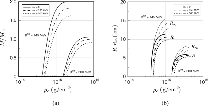
Figure 1: (a) Mass of the star as a function of central density and (b) radius of the star as a function of central density (thick lines) for $B^{1/4}=145$ MeV and $200$ MeV. Thin lines denote the radiation radius $R_{\infty}$. Here we adopt three cases of the $s$ quark mass: i.e., $m_{s}=0$ (solid line), $150$ MeV (dashed line), and $300$ MeV (dotted line). We adopt $\alpha_{c}=0.6$ as a value of the fine structure constant in QCD.

In Fig. 1, we plot several sequences of quark star models with different values of the bag constant $B$ and the $s$ quark mass $m_{s}$. Here we have fixed the fine structure constant in QCD as $\alpha_{c}=0.6$ because the dependence of properties of quark stars on $\alpha_{c}$ is weak, as indicated in Ref. Kohri:2002hf . Therefore we deal with stellar models only for the case of $\alpha_{c}=0.6$ in this paper. In Fig. 1(a) we plot the mass $M/M_{\odot}$ of the star as a function of central density $\rho_{c}$. Here we set $B^{1/4}=145$, $200$ MeV and $m_{s}=0$, $150$, $300$ MeV, respectively. In Fig. 1(b) we also plot the radius of the star as a function of central density by thick lines. Thin lines denote the radiation radius $R_{\infty}$. In Fig. 1, the solid line, dashed line, and dotted line correspond to the cases of $m_{s}=0$, $150$, and $300$ MeV, respectively. In Tables 2 and 3, we list several properties of quark stars whose radiation radii are within the range of $R_{\infty}=3.8$–$8.2$ km, which was reported by Ref. Drake:2002bj .

III Determination of the QNM

Since we are interested in the dependence of QNMs on the EOS of quark matter, we consider only polar perturbation. If we adopt the Regge-Wheeler gauge, the metric perturbation is given by

$$g_{\mu\nu}=g^{(B)}_{\mu\nu}+\left(\begin{array}[]{cccc}r^{l}\hat{H}e^{2\Phi}&i\omega r^{l+1}\hat{H}_{1}&0&0\\ i\omega r^{l+1}\hat{H}_{1}&r^{l}\hat{H}e^{2\Lambda}&0&0\\ 0&0&r^{l+2}\hat{K}&0\\ 0&0&0&r^{l+2}\hat{K}\sin^{2}\theta\end{array}\right)Y^{l}_{m}\,e^{i\omega t},$$ (16)

where $g^{(B)}_{\mu\nu}$ is the background metric (1) of a spherically symmetric star and $\hat{H}$, $\hat{H}_{1},$ and $\hat{K}$ are perturbed metric functions with respect to $r$. We apply a formalism developed by Lindblom and Detweiler Lindblom1985 for relativistic nonradial stellar oscillations. The components of the Lagrangian displacement of fluid perturbations are expanded as

$$\xi^{r} = \frac{r^{l}}{r}e^{\Lambda}\hat{W}Y^{l}_{m}\,e^{i\omega t},$$ (17)

$$\xi^{\theta} = -\frac{r^{l}}{r^{2}}e^{\Lambda}\hat{V}\frac{\partial}{\partial\theta}Y^{l}_{m}\,e^{i\omega t},$$ (18)

$$\xi^{\phi} = -\frac{r^{l}}{r^{2}\sin^{2}\theta}e^{\Lambda}\hat{V}\frac{\partial}{\partial\phi}Y^{l}_{m}\,e^{i\omega t},$$ (19)

where $\hat{W}$ and $\hat{V}$ are functions of $r$.

Assuming that the matter is a perfect fluid and the perturbation is adiabatic, we have the following perturbation equations derived from Einstein equations:

$$\frac{d\hat{H}_{1}}{dr}=-\frac{1}{r}\left[l+1+\frac{2m}{r}e^{2\Lambda}+4\pi r^{2}(P-\rho)e^{2\Lambda}\right]\hat{H}_{1}$$

$$\hskip 34.14322pt+\frac{1}{r}e^{2\Lambda}\left[\hat{H}+\hat{K}+16\pi(P+\rho)\hat{V}\right],$$ (20)

$$\frac{d\hat{K}}{dr}=\frac{l(l+1)}{2r}\hat{H}_{1}+\frac{1}{r}\hat{H}-\left(\frac{l+1}{r}-\frac{d\Phi}{dr}\right)\hat{K}+\frac{8\pi}{r}(P+\rho)e^{\Lambda}\hat{W},$$ (21)

$$\frac{d\hat{W}}{dr}=-\frac{l+1}{r}\hat{W}+re^{\Lambda}\left[\frac{1}{\gamma P}e^{-\Phi}\hat{X}-\frac{l(l+1)}{r^{2}}\hat{V}-\frac{1}{2}\hat{H}-\hat{K}\right],$$ (22)

$$\frac{d\hat{X}}{dr}=-\frac{l}{r}\hat{X}+(P+\rho)e^{\Phi}\biggl{[}\frac{1}{2}\left(\frac{d\Phi}{dr}-\frac{1}{r}\right)\hat{H}-\frac{1}{2}\left(\omega^{2}re^{-2\Phi}+\frac{l(l+1)}{2r}\right)\hat{H}_{1}$$

$$\hskip 34.14322pt+\left(\frac{1}{2r}-\frac{3}{2}\frac{d\Phi}{dr}\right)\hat{K}-\frac{l(l+1)}{r^{2}}\frac{d\Phi}{dr}\hat{V}$$

$$\hskip 34.14322pt-\frac{1}{r}\left(\omega^{2}e^{-2\Phi+\Lambda}+4\pi(P+\rho)e^{\Lambda}-r^{2}\left\{\frac{d}{dr}\left(\frac{1}{r^{2}}e^{-\Lambda}\frac{d\Phi}{dr}\right)\right\}\right)\hat{W}\biggr{]},$$ (23)

$$\biggl{[}1-\frac{3m}{r}-\frac{l(l+1)}{2}-4\pi r^{2}P\biggr{]}\hat{H}-8\pi r^{2}e^{-\Phi}\hat{X}$$

$$\hskip 34.14322pt+r^{2}e^{-2\Lambda}\left[\omega^{2}e^{-2\Phi}-\frac{l(l+1)}{2r}\frac{d\Phi}{dr}\right]\hat{H}_{1}$$

$$\hskip 34.14322pt-\left[1+\omega^{2}r^{2}e^{-2\Phi}-\frac{l(l+1)}{2}-\left(r-3m-4\pi r^{3}P\right)\frac{d\Phi}{dr}\right]\hat{K}=0,$$ (24)

$$\hat{V}=\frac{e^{2\Phi}}{\omega^{2}(P+\rho)}\left[e^{-\Phi}\hat{X}+\frac{1}{r}\frac{dP}{dr}e^{-\Lambda}\hat{W}+\frac{1}{2}(P+\rho)\hat{H}\right],$$ (25)

where $\gamma$ is the adiabatic index of the unperturbed stellar model, which is given by

$$\gamma=\frac{\rho+P}{P}\frac{dP}{d\rho}.$$ (26)

Furthermore, if the proper boundary conditions are imposed on the above perturbation equations, the problem to solve becomes an eigenvalue one. These boundary conditions are given as follows: (i) the eigenfunctions are regular at the stellar center, (ii) the Lagrangian perturbation of pressure vanishes at the stellar surface, and (iii) the gravitational wave is only an outgoing one at infinity. The QNMs of quark stars are determined by solving this eigenvalue problem, and $\omega$ is the eigenvalue of the above perturbation equations. For the treatment of the boundary condition at infinity, we adopt the method of continued-fraction expansion proposed by Leaver Leaver1985 . The detailed method of determining QNMs is given in Sotani2003 ; Sotani2001 .

IV Numerical results

IV.1 $f$ mode

As for gravitational wave radiation emitted from a compact star, there exist QNMs which correspond to each $l$. In this paper, for simplicity we discuss such QNMs only for $l=2$, which would be a dominant mode in a weak field regime.

Compared with the other QNMs, we might relatively easily detect the $f$ mode because its frequency and damping rate are approximately within the sensitivity band of gravitational wave interferometers: e.g., LIGO and so on. Therefore, first we discuss the possibility of constraining parameters of bag models by using the $f$ mode data. When we discuss the observational data of frequency Re($\omega$) and damping rate Im($\omega$) of the $f$ mode, we should bear in mind that the observational data of frequency will be far more accurate than that of damping rate. It was discussed in Ref. Kokkotas2001 that the relative error of the frequency will be about three orders of magnitude smaller than that of the damping rate. To get an insight into the dependence of the $f$ mode on the bag constant $B$ and the $s$ quark mass $m_{s}$, we compute the $f$ mode for each stellar model in Tables 2 and 3.

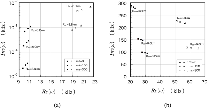
Figure 2: Complex frequencies of (a) $f$ mode and (b) the lowest $w_{\rm II}$ mode for $l=2$. The squares, circles and triangles represent $m_{s}=0$, $150$ MeV and $300$ MeV, respectively. In each panel, the solid (open) marks denote the case of $B^{1/4}=145$ MeV ($200$ MeV).

In Fig. 2(a) we plot the complex frequencies of $f$ mode for $l=2$. In the figure, the squares, circles, and triangles represent $m_{s}=0$, $150$, and $300$ MeV, respectively, and the solid (open) marks denote the case of $B^{1/4}=145$ MeV ($200$ MeV). In Ref. Sotani2003 the authors did not consider such $m_{s}$ dependence because they simply assumed that $m_{s}=0$ as their first step in the paper. From Fig. 2(a), however, we find that both the frequencies and damping rates change at about $10\%$ as $m_{s}$ changes from zero to $300$ MeV for each $B$, and we see that it is important for us to include such effects of nonzero values of $m_{s}$ in bag models to predict the $f$ mode.

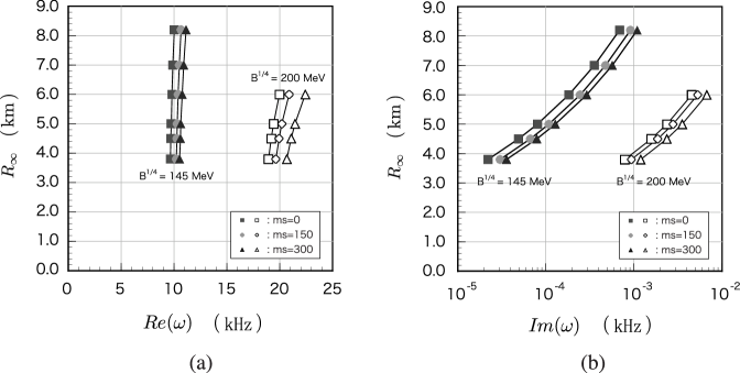
Figure 3: Radiation radius as a function of (a) frequency Re($\omega$) and (b) damping rate Im($\omega$) of $f$ mode for $l=2$. In each figure, the solid and open marks denote $B^{1/4}=145$ MeV and $200$ MeV, respectively.

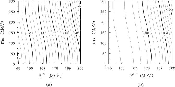
Figure 4: (a) Contours of frequency Re($\omega$) and (b) damping rate Im($\omega$) of $f$ mode for $l=2$ in ($B^{1/4}$, $m_{s}$) plane. Here we adopt the radiation radius as $R_{\infty}=6.0$ km. The numbers with the curve denote the value of frequency Re($\omega$) or damping rate Im($\omega$) in units of kHz.

In Fig. 3 we plot the radiation radius as a function of the (a) frequency Re($\omega$) and (b) damping rate Im($\omega$) of the $f$ mode for $l=2$. In each panel, the solid and open marks denote $B^{1/4}=145$ MeV and $200$ MeV, respectively. From Fig. 3(b) we see that the damping rate is very sensitive to the radiation radius, unlike the frequency in Fig. 3(a). If we observe the damping rate of the $f$ mode within $20\%$, the radiation radius can be determined within $10\%$ as a function of $B$, independently of the value of $m_{s}$. On the other hand, from Fig. 3(a) we see that if we observe the frequency within about $20\%$, for example, we can determine the value of $B$ with reasonable accuracy by using the simultaneously obtained radiation radius from Fig. 3(b). To demonstrate that, we investigate the dependence of the $f$ mode on both the bag constant and the $s$ quark mass when we fix the radiation radius as $R_{\infty}=6.0$ km. In Fig. 4, we plot the contours of the (a) frequency Re($\omega$) and (b) damping rate Im($\omega$) of the $f$ mode for $l=2$ in the ($B^{1/4}$, $m_{s}$) plane. The numbers on the curves denote the value of frequency Re($\omega$) or damping rate Im($\omega$) in units of kHz. We should note that each contour line is nearly parallel to the vertical axis in both Figs. 4(a) and 4(b). This implies that we can obtain a stringent constraint on the bag constant. Indeed, Fig. 4(a) shows that if the frequency of the $f$ mode is detected within $20\%$, then we can determine the value of the bag constant within about $15\%$ independently of the value of the $s$ quark mass.

IV.2 The lowest $w_{\rm II}$ mode

In general, there exist infinite number of $w$ modes and several $w_{\rm II}$ modes for each $l$. As was clearly shown by numerical analysis in Ref. Sotani2003 , however, the $w$ modes are insensitive to the parameters in bag models in which we are interested here. Therefore, we do not adopt $w$ modes in this study. In addition, only one $w_{\rm II}$ mode was found in each quark star model adopted in this study. That is because the “compactness”- i.e., mass to radius ratio—of the adopted quark stars is much smaller than that of standard neutron stars (see Tables 2 and 3). Here, for simplicity we deal with only the lowest $w_{\rm II}$ mode for $l=2$ footnote2 .

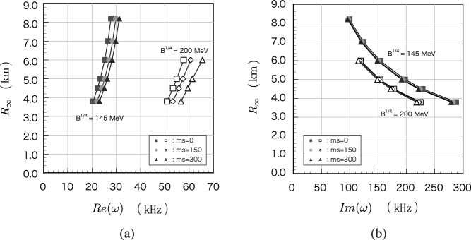
Figure 5: Radiation radius as a function of (a) frequency Re($\omega$) and (b) damping rate Im($\omega$) of the lowest $w_{\rm II}$ mode for $l=2$. In each figure, the solid marks and open ones denote $B^{1/4}=145$ MeV and $200$ MeV, respectively.

In Fig. 2(b) we plot the complex frequencies of the the lowest $w_{\rm II}$ mode. From Fig. 2(b), we see that the $m_{s}$ dependence on the complex frequencies is important, although it was not considered in Ref. Sotani2003 . In Fig. 5 we plot the radiation radius as a function of the (a) frequency Re($\omega$) and (b) damping rate Im($\omega$). The notes on the marks are the same as those in Fig. 3. This figure tells us that it has the same tendency which appears in the case of the $f$ mode; namely, the damping rate is very sensitive to the radiation radius, unlike the frequency. Thus, if we directly observe the damping rate, we can constrain the radiation radius of the quark star.

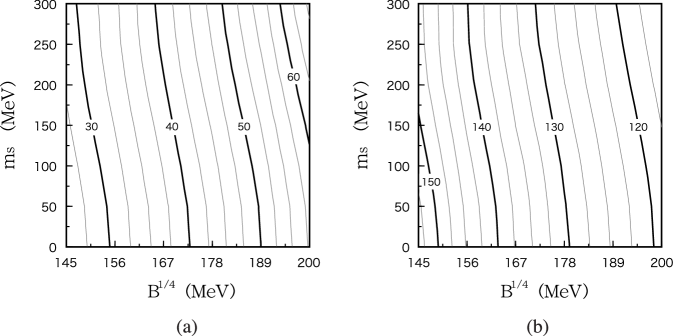
Figure 6: (a) Contours of frequency Re($\omega$) and (b) damping rate Im($\omega$) of the lowest $w_{\rm II}$ mode for $l=2$ in ($B^{1/4}$, $m_{s}$) plane. Here we adopt the radiation radius as $R_{\infty}=6.0$ km. The numbers with the curve denote the value of frequency Re($\omega$) or damping rate Im($\omega$) in units of kHz.

Furthermore, along with the case of the $f$ mode, we plot the contour of the frequency and the damping rate of the lowest $w_{\rm II}$ mode in the ($B^{1/4}$, $m_{s}$) plane in Fig. 6. By using the lowest $w_{\rm II}$ mode, we are able to develop a similar argument as that discussed in the case of the $f$ mode and get an independent constraint on the bag constant and $s$ quark mass.

However, we should keep in mind that even if a large amount of energy is released through these modes, accurate observation of the $w$ and $w_{\rm II}$ modes may be difficult. That is because both the frequency and damping rate of these modes are larger than the sensitivity ranges of gravitational wave interferometers Andersson1996 . Thus we would mainly use the observational data of the $f$ mode to obtain information about the bag model parameters. Then we could subsidiarily use the data on the lowest $w_{\rm II}$ mode. It should be noted that, since Fig. 6 has similar features found in the $f$ mode, even if we combine it with information from the $f$ mode, we may not have strict constraints on both $m_{s}$ and $B$, independently. There exists an essential degeneracy in $f$ and the lowest $w_{\rm II}$ mode QNMs because the configuration of the contour of Fig. 4 is very similar to that of Fig. 6.

V Conclusion

We have discussed how we can obtain information about the EOS of quark matter by using future observations of gravitational waves emitted from quark stars. In particular we have studied the EOS in bag models and assumed that the star is a pure quark star. We have computed the QNMs—i.e., the $f$ and the lowest $w_{\rm II}$ modes—in several quark star models. We have demonstrated that by comparing the results of theoretical computations with the observational data of the $f$ mode and the lowest $w_{\rm II}$ modes we can obtain constraints on the bag constant $B$ and $s$ quark mass $m_{s}$.

If we have the damping rate—i.e., Im($\omega$)—of the $f$ mode within $20\%$, the radiation radius of the quark star can be determined within about $10\%$ including the uncertainty of the $s$ quark mass. Furthermore if we also obtain the frequency—i.e., Re($\omega$)—of the $f$ mode within $20\%$, the value of the bag constant can be determined within about $15\%$, independently of the uncertainty of the $s$ quark mass, by using the simultaneously obtained radiation radius. Concerning the lowest $w_{\rm II}$ mode, we can also develop a similar argument as in the case of the $f$ mode and get independent constraints on the model parameters. However, note that it is relatively difficult to detect the lowest $w_{\rm II}$ mode by the future planned gravitational wave interferometers whose frequency ranges are not very sensitive to the lowest $w_{\rm II}$ mode. Therefore, such data will be subsidiarily used in statistical analyses. It should be also noted that there is a degeneracy in the dependence of $f$ and the lowest $w_{\rm II}$ mode QNM complex frequencies on the bag model parameters $m_{s}$ and $B$. As for high frequency gravitational waves, a dual-type detector has been proposed, which would reach very good spectral strain sensitivities ($\sim 2\times 10^{-23}\ \mbox{Hz}$) in a considerable broadband (between $1$ and $3\ \mbox{kHz}$) Cerdonio2001 and then open a new interesting window to the QNMs of compact objects.

As long as we have data with tolerable accuracy in future, we will be able to perform statistical analyses to fit them and get constraints on both the bag constant and the $s$ quark mass. If we have further information about the bag constant or the $s$ quark mass by utilizing the EOS models based on future developments in an effective theory of QCD, such as perturbation theories or finite-temperature lattice data, we can constrain them more strictly. Including independent observations of the radiation radius—e.g., sorts of X-ray observations—would also support us in inferring the bag model parameters. QNMs from compact stars will be observed in the near future and deepen our understanding of hadron physics and QCD.

Table 1: Bag model parameters fitted to hadron mass spectra.

	$B^{1/4}$ (MeV)	$m_{s}$ (MeV)	$\alpha_{c}$	Reference
	145	279	2.2	DeGrand:cf
	200–220	288	0.8–0.9	Carlson:er
	149	283	2.0	Bartelski:1983cc

Table 2: Properties of quark stars in the case of $B^{1/4}=145\,\,\text{MeV}$. Here, $R_{\infty}$, $m_{s}$, $\rho_{c}$, $M/M_{\odot}$, $R$, and $M/R$ are the radiation radius, the $s$ quark mass, the central density, the mass in units of $M_{\odot}$, the radius, and the compactness of the star, respectively.

$R_{\infty}\,\,(\text{km})$	$m_{s}\,\,(\text{MeV})$	$\rho_{c}\,\,(\text{g/cm}^{3})$	$M/M_{\odot}$	$R\,\,(\text{km})$	$M/R$
$3.800$	$0.0$	$4.221\times 10^{14}$	$4.539\times 10^{-2}$	$3.731$	$1.796\times 10^{-2}$
$3.800$	$150.0$	$4.714\times 10^{14}$	$5.020\times 10^{-2}$	$3.724$	$1.991\times 10^{-2}$
$3.800$	$300.0$	$5.027\times 10^{14}$	$5.305\times 10^{-2}$	$3.719$	$2.106\times 10^{-2}$
$6.000$	$0.0$	$4.412\times 10^{14}$	$1.678\times 10^{-1}$	$5.735$	$4.320\times 10^{-2}$
$6.000$	$150.0$	$4.979\times 10^{14}$	$1.846\times 10^{-1}$	$5.706$	$4.778\times 10^{-2}$
$6.000$	$300.0$	$5.392\times 10^{14}$	$1.951\times 10^{-1}$	$5.688$	$5.066\times 10^{-2}$
$8.200$	$0.0$	$4.731\times 10^{14}$	$3.925\times 10^{-1}$	$7.544$	$7.684\times 10^{-2}$
$8.200$	$150.0$	$5.436\times 10^{14}$	$4.293\times 10^{-1}$	$7.472$	$8.483\times 10^{-2}$
$8.200$	$300.0$	$6.049\times 10^{14}$	$4.540\times 10^{-1}$	$7.423$	$9.031\times 10^{-2}$

Table 3: Same as Table 2 except for $B^{1/4}=200\,\,\text{MeV}$.

$R_{\infty}\,\,(\text{km})$	$m_{s}\,\,(\text{MeV})$	$\rho_{c}\,\,(\text{g/cm}^{3})$	$M/M_{\odot}$	$R\,\,(\text{km})$	$M/R$
$3.800$	$0.0$	$1.660\times 10^{15}$	$1.477\times 10^{-1}$	$3.560$	$6.125\times 10^{-2}$
$3.800$	$150.0$	$1.796\times 10^{15}$	$1.563\times 10^{-1}$	$3.544$	$6.513\times 10^{-2}$
$3.800$	$300.0$	$2.019\times 10^{15}$	$1.692\times 10^{-1}$	$3.520$	$7.098\times 10^{-2}$
$6.000$	$0.0$	$2.038\times 10^{15}$	$4.742\times 10^{-1}$	$5.113$	$1.369\times 10^{-1}$
$6.000$	$150.0$	$2.285\times 10^{15}$	$4.977\times 10^{-1}$	$5.052$	$1.455\times 10^{-1}$
$6.000$	$300.0$	$2.781\times 10^{15}$	$5.344\times 10^{-1}$	$4.953$	$1.593\times 10^{-1}$