Improving the sensitivity to gravitational-wave sources by modifying the input-output optics of advanced interferometers

Abstract

To improve the sensitivity of laser-interferometer gravitational-wave (GW) detectors, experimental techniques of generating squeezed vacuum in the GW frequency band are being developed. The squeezed vacuum generated from non-linear optics have constant squeeze angle and squeeze factor, while optimal use of squeezing usually requires frequency dependent (FD) squeeze angle and/or homodyne detection phase. This frequency dependence can be realized by filtering the input squeezed vacuum or the output light through detuned Fabry-Perot cavities. In this paper, we study FD input-output schemes for signal-recycling interferometers, the baseline design of Advanced LIGO and the currently operational configuration of GEO 600. Complementary to a recent proposal by Harms et al. to use FD input squeezing and ordinary homodyne detection, we explore a scheme which uses ordinary squeezed vacuum, but FD readout. Both schemes, which are sub-optimal among all possible input-output schemes, provide a global noise suppression by the power squeeze factor. At high frequencies, the two schemes are equivalent, while at low frequencies the scheme studied in this paper gives better performance than the Harms et al. scheme, and is nearly fully optimal. We then study the sensitivity improvement achievable by these schemes in Advanced LIGO era (with 30-m filter cavities and current estimates of filter-mirror losses and thermal noise), for neutron star binary inspirals, for low-mass X-ray binaries and known radio pulsars. Optical losses are shown to be a major obstacle for the actual implementation of these techniques in Advanced LIGO. On time scales of third-generation interferometers, like EURO/LIGO-III ($\sim 2012$), with kilometer-scale filter cavities and/or mirrors with lower losses, a signal-recycling interferometer with the FD readout scheme explored in this paper can have performances comparable to existing proposals.

I Introduction

The first generation of kilometer-scale, ground-based laser-interferometer gravitational-wave (GW) detectors (interferometers for short), located in the United States (LIGO LIGO ; S1inst ), Europe (VIRGO VIRGO and GEO 600 GEO ; S1inst ) and Japan (TAMA 300 TAMA ), have begun their search for gravitational radiation and have yielded first scientific results S1continuous ; S1inspiral ; S1burst ; S1stochastic . The development of interferometers of the second generation, such as Advanced LIGO (to be operative around 2008 ALIGO ), and future generations (such as EURO and LIGO-III), is underway. In this paper we explore the possibility of improving the sensitivity of signal-recycling (SR) interferometers SR ; M95 , the baseline design of Advanced LIGO ALIGO and the current optical configuration of GEO 600 GEO , when squeezed vacuum is injected into the antisymmetric port (the “input port”, as we shall refer to it in this paper).

In the early 1980s, building on works of Caves Caves , Unruh Unruh proposed the first design of a squeezed-input interferometer, which can beat the free-mass Standard Quantum Limit (SQL) SQL . Other theoretical studies of input squeezing followed Others . If generated from non-linear optics, squeezed vacuum will have frequency independent squeeze angle and squeeze factor in the GW frequency band SQZ . The above theoretical works, as well as past experiments employing squeezed vacuum to enhance interferometer performances SQZexp , all assume frequency independent squeezing. In the 1990s, Vyatchanin, Matsko and Zubova FDH realized that the sensitivity of GW interferometers can also be improved, beating the SQL, by measuring an optimal output quadrature, which is usually frequency dependent. Later, Kimble, Levin, Matsko, Thorne and Vyatchanin (KLMTV) KLMTV00 made a comprehensive, unified theoretical study of improving the sensitivity of conventional interferometers by injecting squeezed vacuum into the input port and/or performing frequency dependent (FD) homodyne detection at the output port. They showed that, for conventional interferometers, in order to obtain a noise suppression proportional to the power squeeze factor at all frequencies (optimal input squeezed vacuum), either the squeezed vacuum must have a FD squeeze angle (squeezed-input interferometer), or FD homodyne detection has to be applied at the output port (squeezed-variational interferometer). [Of course, combinations of those optical configurations can also be used, but they will be experimentally more challenging.] KLMTV proposed a practical way of implementing FD homodyne detection, as well as converting squeezed vacuum with constant squeeze angle into squeezed vacuum with FD squeeze angle, by filtering the output light or input squeezed vacuum through two detuned (with respect to the laser carrier frequency) FP cavities (KLMTV filters). KLMTV constructed the explicit filter parameters that provide the desired frequency dependence for squeezed-input and squeezed-variational interferometers, showing that the latter provides a better ideal performance than the former, but is more susceptible to optical losses. Purdue and Chen (PC) studied the KLMTV filters further, and worked out the most general FD squeeze angle and homodyne phase that a sequence of filters can provide PC02 .

Experimental programs on generating squeezed vacuum in the GW frequency band and injecting it into GW interferometers have already started in several groups, for example, at the Australian National University ANU , at the Massachusetts Institute of Technology, USA CM , and at the Albert Einstein Institut in Hannover, Germany AEI . Their goal in the next several years is to inject squeezed vacuum with $\sim$10 dB squeeze factor (as a net result after optical losses) into an interferometer. It is very likely that the squeezed vacuum they obtain has a constant squeeze angle in the GW frequency band.

This paper contains three relatively independent parts. In the first part, we generalize the work by KLMTV on FD input-output optics to SR interferometers. Recently, Harms et al. Harms03 applied the KLMTV squeezed-input scheme, combining FD input squeezed vacuum with ordinary homodyne detection to SR interferometers, achieving a global noise suppression equal to the power squeeze factor. Harms et al. also showed that their FD squeezed-input scheme is only sub-optimal; the fully optimal scheme, however, requires complicated frequency dependence in both input squeeze angle and homodyne phase, and cannot be achieved by KLMTV filters. Complementary to Harms et al.’s scheme, we explore here the scheme which combines ordinary input squeezed vacuum with FD homodyne detection (henceforth, the BC scheme). This scheme, which can be thought of as a generalization of the KLMTV squeezed-variational scheme, can also provide a global noise suppression by the power squeeze factor. In addition, at high frequencies (above $\sim 200$Hz for typical Advanced LIGO configurations), it is equivalent to the Harms et al. scheme, while at low frequencies (below $\sim 200$ Hz) it is to a very good approximation fully optimal, and thus provides a better sensitivity than the Harms et al. scheme.

In the second part of this paper we apply these FD input-output schemes to Advanced LIGO (2008), assuming that the generation and injection of squeezed vacuum might have already (or partially) become available at that time scale. The major obstacle in using FD input-output techniques in the facilities of Advanced LIGO is the constraint that the filter cavities cannot be longer than $\sim$30 meters — the shorter the filter cavities, the larger the optical losses. In our analyses we assume that filter losses dominate over internal interferometer losses, and comment only briefly on the effects of the latter. To quantify the improvement in sensitivity due to FD techniques, we consider three classes of astrophysical sources: neutron-star (NS) binary inspirals, low-mass X-ray binaries (LMXBs) and known radio pulsars. In addition to the ideal quantum noise and filter optical losses, we also take into account current estimates of thermal and seismic noises. [We note that GW interferometers can already take advantage of input squeezed vacuum even without using FD techniques, if the interferometer parameters are carefully optimized. For example, an interesting optical configuration without FD input-output optics has been explored by Corbitt and Mavalvala CM , providing good sensitivities at high frequencies.]

In the third part of the paper, we apply our FD readout scheme to third-generation interferometers, such as EURO/LIGO-III, which are scheduled to be operative around 2012. We assume that on this time scale, due to the implementation of cryogenic techniques and the use of kilometer-length KLMTV filters, thermal noise will be negligible and loss effects will be rather low. Third-generation interferometers will have to beat the SQL significantly. We compare the performance of SR interferometers with our FD readout scheme with those of other existing SQL-beating proposals, such as the KLMTV squeezed-variational interferometer KLMTV00 and the speed-meter interferometers ligoIII:sm ; ligoIII:sag . We also investigate the accuracy of short-arm and short-filter approximations used in describing GW interferometers and KLMTV filters. More dramatic ideas to circumvent the SQL in GW interferometers exist, for example, the intra-cavity schemes of Braginsky, Gorodetsky and Khalili K03 , and the feed-back control scheme of Courty, Heidmann and Pinard CHP . Since thorough analyses of these schemes tuned to GW interferometers has not been available yet, in this paper we do not compare the performances.

Quantity	Symbol and Value
Laser frequency	$\omega_{0}=1.8\times 10^{15}\,{\rm sec}^{-1}$
GW sideband frequency	$\Omega$
Arm-cavity length	$L$ ($4\,{\rm km}$ for LIGO facilities)
Mirror mass	$m$ ($40\,$kg for Advanced LIGO)
Input test-mass (ITM) power transmissivity (LIGO only)	$T$
Arm-cavity circulating power	$I_{c}$ ($840\,$kW for Advanced LIGO)
Light power at the beamsplitter	$I_{0}$
SR optical resonant (sideband) frequency	$-\lambda$
SR bandwidth	$\epsilon$
Homodyne detection phase	$\zeta$
Input squeeze factor	$r$
Input squeeze angle	$\alpha$

Table 1: Parameters of the SR interferometer and input squeezed vacuum.

Readers with particular interests in the astrophysical consequences of using input squeezed vacuum and FD schemes could go directly to the second part of the paper [Sec. V], in which an in-depth understanding of the optics is not required. The paper is organized as follows. In Sec. II, we write the input-output relation of a non-squeezed SR interferometer in terms of the intrinsic FD rotation angle and ponderomotive squeeze factor. In Sec. III we review the KLMTV filters, including the effects of optical losses. In Sec. IV we study FD input-output schemes for SR interferometers. More specifically, in Sec. IV.1, we write the general input-output relation of SR interferometers with FD input-output optics; in Sec. IV.2, we study all sub-optimal schemes that allow global noise suppression, proposing the BC scheme; in Sec. IV.3 we study the regime with low ponderomotive squeezing (high frequency band of Advanced LIGO), and show the equivalence between the BC and the Harms et al. schemes; in Sec. IV.4 we study the fully optimal scheme, showing that at low frequencies the BC scheme is a good approximation to it. In Sec. V, we investigate the improvement in sensitivity to GWs from various astrophysical sources. In Sec. VI, we compare the BC scheme with other proposals for third-generation interferometers, and study the effect of filter lengths in FD readout schemes. Finally, Sec. VII summarizes our conclusions.

II Quadrature rotation and ponderomotive squeezing in signal recycled interferometers

A summary of the various parameters of SR interferometers, such as Advanced LIGO and GEO 600, is given in Table 1. The input-output relation for the quadrature fields in signal recycled interferometers reads [see, e.g., Eq. (24) in Ref. BC5 , with superscript $(1)$ and tilde dropped]

$$\left(\begin{array}[]{c}{b}_{1}\\ {b}_{2}\end{array}\right)=\frac{1}{{M}}\,\left\{\left(\begin{array}[]{cc}{C}_{11}&{C}_{12}\\ {C}_{21}&{C}_{22}\end{array}\right)\left(\begin{array}[]{c}{a}_{1}\\ {a}_{2}\end{array}\right)+\left(\begin{array}[]{c}{D}_{1}\\ {D}_{2}\end{array}\right)\frac{h}{h_{\rm SQL}}\right\}\,,$$ (1)

where we define

$${M}={\left[\lambda^{2}-(\Omega+i\epsilon)^{2}\right]\,\Omega^{2}-\lambda\,\iota_{c}}\,,$$ (2)

and

$${C}_{11}={C}_{22} = \Omega^{2}(\Omega^{2}-\lambda^{2}+\epsilon^{2})+\lambda\,\iota_{c}\,,$$ (3)

$${C}_{12} = -2\epsilon\,\lambda\,\Omega^{2}\,,$$ (4)

$${C}_{21} = 2\epsilon\,\lambda\,\Omega^{2}-2\epsilon\,\iota_{c}\,,$$ (5)

$${D}_{1}=-2\lambda\,\sqrt{\epsilon\,\iota_{c}}\,\Omega\,,\quad\quad{D}_{2}=2(\epsilon-i\Omega)\,\Omega\,\sqrt{\epsilon\,\iota_{c}}\,.$$ (6)

The parameters $\lambda$ and $\epsilon$ are related to the real and imaginary parts of the free optical resonant frequency $\omega_{\rm free}$ of the SR interferometer by BC5 :

$$\omega_{\mbox{\tiny SR}}^{\rm free}=\omega_{0}-\lambda-i\epsilon\,,$$ (7)

where $\omega_{0}$ is the laser frequency. The parameter $\iota_{c}$ is defined by

$$\iota_{c}=\frac{8\omega_{0}\,I_{c}}{m\,L\,c}$$ (8)

$$\simeq (2\pi\times 100\,{\rm Hz})^{3}\left(\frac{I_{c}}{840\,{\rm kW}}\right)\left(\frac{40\,{\rm kg}}{m}\right)\left(\frac{4\,{\rm km}}{L}\right),$$

where $c$ is the speed of light, $m$ is the mirror mass, $L$ is the arm length, and $I_{c}$ is the circulating optical power in the arm cavity, which in turn depends on the power at beamsplitter, $I_{0}$, by

$$I_{c}=\frac{2}{T}I_{0}\,.$$ (9)

The quantity $\iota_{c}$ must be on the order of $\Omega_{\rm GW}^{3}$ if we want the opto-mechanical coupling to modify the detuned (assuming $\lambda\sim\Omega_{\rm GW}$) interferometer’s sensitivity in the GW frequency band [see Eqs. (3)–(5)]. In addition, we have denoted by

$$h_{\rm SQL}\equiv\sqrt{\frac{8\hbar}{m\Omega^{2}L^{2}}}\,$$ (10)

the free-mass SQL for the gravitational strain $h(\Omega)$.

It is important to note that the input-output relation, as given by Eqs. (1)–(6), has been obtained at the leading order in $\Omega L/c$ (as well as in $\epsilon L/c$, $\lambda L/c$ and $\iota_{c}^{1/3}L/c$). This approximation is called the “short-arm” approximation, since it assumes that the arm length be much smaller than the gravitational wavelength. The short-arm approximation simplifies dramatically the form of the input-output relation, as well as the design of optimal KLMTV filters (as we shall see later in this paper).

In the following sections we first write the input-output $b_{1,2}$-$a_{1,2}$ relation [the first term inside the parenthesis on the RHS of Eq. (1)] in terms of an intrinsic squeeze factor $q$ and an intrinsic rotation angle $\varphi$. We then study how the output quadratures depend on the signal [the second term inside the parenthesis on the RHS of Eq. (1)], obtaining the quadrature $\zeta_{\rm max}$ at which the signal strength is maximal. Finally, we give the noise spectrum, and express it in terms of $q$, $\varphi$ and $\zeta_{\rm max}$.

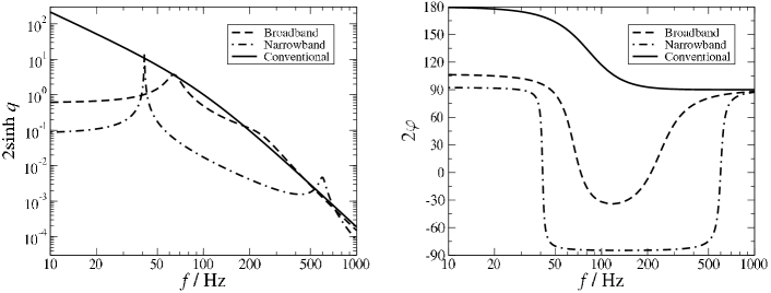
Figure 1: We plot $2\sinh q$ (left panel) and $2\varphi$ (right panel) for two typical SR optical configurations, the broadband with $\lambda=2\pi\times 234.07\,{\rm Hz}$, $\epsilon=2\pi\times 70.36\,{\rm Hz}$, (dashed line) and narrowband with $\lambda=2\pi\times 601.43\,{\rm Hz}$, $\epsilon=2\pi\times 25\,{\rm Hz}$, (dot-dashed line). We also plot the curves for the conventional interferometer with $\lambda=0$, $\epsilon=2\pi\times 93.75\,{\rm Hz}$ (continuous line). In all cases we fix $I_{c}=840\,$kW and $m=40\,$kg.

II.1 Rotation of noise quadratures and ponderomotive squeezing

As is evident from Eqs. (2)–(5), in detuned SR interferometers (with $\lambda\neq 0$), the input-output relation is frequency dependent. For high-power interferometers like Advanced LIGO, the matrix ${C}_{ij}$ contains both a FD rotation and a FD (ponderomotive) squeezing. Let us work these quantities out explicitly. The quantum transfer matrix (with an overall phase factor removed)

$${\cal M}_{ij}=\frac{C_{ij}}{|M|}\,,\quad\quad i,j=1,2\quad(\det{\cal M}_{ij}=1)\,,$$ (11)

is a matrix with real elements and with determinant equal to one BC2 . So, it can always be written in the form

$${\cal M}=\mathbf{R}(\theta)\,\mathbf{S}(\varphi,q)\,,$$ (12)

as a product of a rotation operator $\mathbf{R}(\theta)$ and a squeezing operator $\mathbf{S}(\varphi,q)$, defined by

$$\mathbf{R}(\theta)\equiv\left(\begin{array}[]{rr}\cos\theta&-\sin\theta\\ \sin\theta&\cos\theta\end{array}\right)$$ (13)

and

$$\mathbf{S}(\varphi,q) \equiv \mathbf{R}(\varphi)\,\mathbf{S}(q)\,\mathbf{R}(-\varphi)\,,$$ (14)

$$\mathbf{S}(q) \equiv \left(\begin{array}[]{ll}e^{-q}&\\ &e^{q}\end{array}\right)\,,\quad q\geq 0\,.$$ (17)

Here $\theta$ is the rotation angle, $q$ is the squeeze factor, and $\varphi$ is the squeeze angle. These quantities can in general be frequency dependent. It can be easily shown that the decomposition (12) is also unique, unless $\mathcal{M}$ is a pure rotation (with $q=0$, $\theta$ being the rotation angle, and $\varphi$ being arbitrary). From Eqs. (12)–(14), we have

$${\rm Tr}({\cal M}\,{\cal M}^{\dagger})=2\cosh 2q\,,$$ (18)

which determines $q$ uniquely once ${\cal M}$ is given (recall that $q\geq 0$). If $q$ is zero, $\mathbf{S}(\varphi,q)$ reduces to the identity matrix regardless of the value of $\varphi$ [see Eqs. (14) and (17)], and $\theta$ must be the rotation angle of $\mathcal{M}$; otherwise, in order that $\mathbf{R}(\theta)\mathbf{S}(q,\varphi)=\mathbf{R}(\theta^{\prime})\mathbf{S}(q,\varphi^{\prime})$, one must impose that

$$\theta-\theta^{\prime}=m\pi\,,\qquad\varphi-\varphi^{\prime}=n\pi\,,$$ (19)

where $m$ and $n$ are integers, and $m-n$ must be an even number. The uniqueness of the decomposition (12) assures that the quantities $\theta$, $q$ and $\varphi$ have unambiguous physical meaning.

By comparing Eq. (12) with Eqs. (1)–(5), we can express the angles $\theta,\varphi$ and the factor $q$ in terms of SR parameters. Using the identity (18), we get the squeeze factor $q$:

$$\cosh 2q=1+\frac{2\epsilon^{2}\,\iota_{c}^{2}}{|M|^{2}}\,.$$ (20)

Since for SR interferometers, $C_{11}=C_{22}$, we must impose $\cos(2\varphi+\theta)=0$, or $\theta=\pi/2-2\varphi$. This casts $\mathcal{M}_{ij}$ into the following form:

$$\mathcal{M}$$ (23)

$$= \mathbf{R}(\pi/2-\varphi)\,\mathbf{S}(q)\,\mathbf{R}(-\varphi)$$

$$= \left(\begin{array}[]{cc}\sin 2\varphi\,\cosh q&-\sinh q-\cos 2\varphi\,\cosh q\\ \sinh q-\cos 2\varphi\,\cosh q&\sin 2\varphi\,\cosh q\end{array}\right)\,.$$

Thus we have

$$\tan 2\varphi = -\frac{\mathcal{M}_{11}+\mathcal{M}_{22}}{\mathcal{M}_{12}+\mathcal{M}_{21}}$$ (25)

$$= \frac{\iota_{c}\,\lambda+\Omega^{2}\,(\epsilon^{2}-\lambda^{2}+\Omega^{2})}{\epsilon\,(2\lambda\,\Omega^{2}-\iota_{c})}\,,$$

$$\sinh q = \frac{\mathcal{M}_{21}-\mathcal{M}_{12}}{2}=\frac{\epsilon\,\iota_{c}}{|M|}\,.$$ (26)

Note that Eq. (26) agrees with Eq. (20).

In absence of SR mirror, or when the SR cavity is either resonant or antiresonant with the carrier, we have $\lambda=0$, and the above equations reduce to the known expressions for conventional interferometers KLMTV00

$$\sinh q=\frac{\cal K}{2}\,,\quad\tan 2\varphi=-\frac{2}{\cal K}\,,$$ (27)

with

$${\cal K}=\frac{2\epsilon\,\iota_{c}}{\Omega^{2}\,(\Omega^{2}+\epsilon^{2})}\,,$$ (28)

${\cal K}$ being the coupling constant defined by KLMTV in Eq. (18). The $\sinh q$ in Eqs. (26) and (27) is proportional to $\iota_{c}$, which is in turn proportional to the circulating power $I_{c}$ and inversely proportional to the mirror mass $m$. This means the squeezing arises from the well-known ponderomotive effect BM .

In Fig. 1 we plot $2\sinh q$ (left panel) and $2\varphi$ (right panel) as functions of frequency, for two typical SR configurations and a conventional-interferometer configuration. [Note that $2\sinh q\simeq 2q$ as $q\ll 1$ and $2\sinh q\simeq e^{q}$ as $q\gg 1$.] As we can see from the plots, both $2\sinh q$ and $2\varphi$ are frequency dependent.

Let us focus on the detuned configurations (dash and dash-dot curves in Fig. 1). The squeeze factor decreases at high frequencies. This can be easily understood from Eq. (26), where we see that $\sinh q$ (hence $q$) decreases when $\Omega$ increases, because $M$, Eq. (2), is a polynomial in $\Omega$, so it grows indefinitely as $\Omega$ tends to infinity. [The factor $\Omega^{2}$ in Eq. (2) can be traced back to the response of a free mirror to an external force, which decreases as $1/\Omega^{2}$; while the factor $[\lambda^{2}-(\Omega+i\epsilon)^{2}]$ increases at high frequencies because the storage time ($1/\epsilon$) of the interferometer becomes much longer than the GW period.] Using Eq. (2) and the fact that $|M|\geq\Im(M)$, we obtain

$$|M|\geq 2\,\epsilon\,\Omega^{3}\,.$$ (29)

Combining Eq. (29) with Eqs. (26) and (8), we have

$$\sinh q=\frac{\epsilon\iota_{c}}{|M|} < \frac{\iota_{c}}{2\Omega^{3}}$$ (30)

$$\simeq 2\times 10^{-2}\left(\frac{2\pi\times 300\,{\rm Hz}}{\Omega}\right)^{3}\left(\frac{I_{c}}{840\,{\rm kW}}\right)$$

$$\times\left(\frac{40\,{\rm kg}}{m}\right)\left(\frac{4\,{\rm km}}{L}\right)\,.$$

This gives an upperbound for the amount of squeezing achievable with a given optical power, regardless of resonant features. As we can see from Eq. (30), even for Advanced LIGO optical power, at frequencies larger than $\sim 300$ Hz, the intrinsic ponderomotive squeezing is already very small.

From the left panel in Fig. 1 we observe that the squeeze factor is amplified significantly near the “optical spring” resonance  (left peaks), and mildly near the optical resonance (right peaks). Those resonant features in $q$ are caused by local minima of $M$ around the two resonant frequencies; the optical resonance provides less squeezing since squeezing is already suppressed at such high frequencies [see Eq. (30)]. The squeeze factor tends to a nonzero constant for $\Omega$ much lower than the resonant frequencies. By taking the limit of Eq. (26) when $\Omega\rightarrow 0$ we obtain that the constant value is:

$$\sinh\left[q(\Omega=0)\right]=\frac{\epsilon}{\lambda}\,.$$ (31)

From the right panel of Fig. 1, we see that the rotation angle $2\varphi$ changes by $180^{\circ}$ across both the optical-spring resonant frequency and the optical resonant frequency. The above features in $2\varphi$ are typical of resonators and can be explained easily from Eq. (25).

For conventional interferometers ($\lambda=0$; continuous curves in Fig. 1), the squeeze factor $q$ becomes larger as $\Omega$ decreases, providing the strongest squeezing at almost all frequencies. In particular, $q\rightarrow+\infty$ when $\Omega\rightarrow 0$, as we can see from Eq. (31). The rotation angle $2\varphi$ changes by $180^{\circ}$ only once over the entire frequency band.

In the low-power limit ($I_{c}\rightarrow 0$, such that $q\rightarrow 0$), the transfer matrix $\mathcal{M}$ reduces to the rotation matrix

$$\mathcal{M}_{\mbox{\scriptsize low-power}}=\mathbf{R}(\pi/2-\varphi_{\mbox{\scriptsize low-power}})\,,$$ (32)

with

$$\tan\left(\frac{\pi}{2}-2\,\varphi_{\mbox{\scriptsize low-power}}\right)=\frac{2\lambda\,\epsilon}{\Omega^{2}-\lambda^{2}+\epsilon^{2}}\,.$$ (33)

Note that this low-power approximation also applies to high frequencies where ponderomotive squeezing is suppressed, even when the power is the typical high power in Advanced LIGO [see Fig. 1 and Eqs. (30)].

II.2 Rotation of signal quadrature

Now suppose the output quadrature

$$b_{\zeta}=b_{1}\,\sin\zeta+b_{2}\,\cos\zeta$$ (34)

is measured, then the signal part of $b_{\zeta}$ [second term inside the parenthesis on the RHS of Eq. (1)] is

$$s_{\zeta}\propto D_{1}\,\sin\zeta+D_{2}\,\cos\zeta\propto-\lambda\,\sin\zeta+(\epsilon-i\Omega)\,\cos\zeta\,.$$ (35)

Taking the magnitude squared of the above equation, we obtain the signal power in this quadrature,

$$|s_{\zeta}|^{2}$$ (36)

$$\propto (\Omega^{2}+\lambda^{2}+\epsilon^{2})+(\Omega^{2}-\lambda^{2}+\epsilon^{2})\,\cos 2\zeta-2\lambda\,\epsilon\,\sin 2\zeta$$

$$= S_{0}+S_{1}\cos 2(\zeta-\zeta_{\rm max})\,,$$

where

$$S_{0} \equiv (\Omega^{2}+\lambda^{2}+\epsilon^{2})\,,$$ (37)

$$S_{1} \equiv \sqrt{(\Omega^{2}+\lambda^{2}+\epsilon^{2})^{2}-4\lambda^{2}\,\Omega^{2}}\,,$$ (38)

and

$$\zeta_{\rm max}=\frac{1}{2}\arctan\frac{-2\lambda\,\epsilon}{\Omega^{2}-\lambda^{2}+\epsilon^{2}}$$ (39)

is the quadrature with maximun signal power. Note that the relative signal strengths in different quadratures depend on $\epsilon$ and $\lambda$ (i.e., on the optical properties of the interferometer), but not on $\iota_{c}$ (i.e., on the laser power and mirror masses). Equation (39) suggests a resonant feature of $\zeta_{\rm max}$ near the optical resonant frequency, $\Omega\sim|\lambda|$. Equations (36)–(38) also show clearly a known result BC2 : if $\lambda\,\Omega\neq 0$, we have $S_{0}>S_{1}$, so it is impossible to have an output quadrature with no signal.

By comparing Eqs. (33) and (39), we can relate the frequency dependence of the maximal-signal quadrature of an interferometer with arbitrary optical power to the noise-quadrature rotation of the corresponding low-power interferometer, that is

$$\zeta_{\rm max}=-\frac{1}{2}\left(\frac{\pi}{2}-2\,\varphi_{\mbox{\scriptsize low-power}}\right)\,.$$ (40)

As we shall see in Sec. III, the factor of $1/2$ in front of the RHS of the above equation makes it difficult to design optimal FD schemes near the optical resonant frequency.

II.3 Noise Spectral Density

Assuming that ordinary vacuum enters the input port, the SR noise spectral density in the $\zeta$ quadrature (34) is given by [see e.g., Eqs. (22)–(36) in Ref. BC5 ]

$$S_{h}=\frac{h_{\rm SQL}^{2}}{\left|D_{1}\,\sin\zeta+D_{2}\,\cos\zeta\right|^{2}}\,\times$$

$$[\left(C_{11}\,\sin\zeta+C_{21}\,\cos\zeta\right)^{2}+\left(C_{12}\,\sin\zeta+C_{22}\,\cos\zeta\right)^{2}]\,.$$

By expressing $S_{h}$ in terms of the quantities $\varphi$, Eq. (25), $q$, Eq. (26), $\zeta_{\rm max}$, Eq. (39), and $S_{0,1}$, Eqs. (37) and (38), we obtain:

$$S_{h}=|M|^{2}\,\frac{\left[\cosh 2q-\sinh 2q\,\cos 2(\zeta-\varphi)\right]}{4\epsilon\,\iota_{c}\,\Omega^{2}\,\left[S_{0}+S_{1}\cos 2(\zeta-\zeta_{\rm max})\right]}\,h_{\rm SQL}^{2}\,.$$ (42)

III Frequency dependent input-output optics using KLMTV filters

Quantity	Symbol
Filter Length	$L_{f}$
Input-mirror power transmissivity and reflectivity	$T_{i}$, $R_{i}=1-T_{i}$
End-mirror power transmissivity and reflectivity	$T_{e}$, $R_{e}=1-T_{e}$
Resonant (sideband) frequency	$\omega_{f}$
Bandwidth	$\gamma_{f}$

Table 2: Parameters of an optical filter.

To realize FD homodyne detection and generate squeezed vacuum with FD squeeze angle KLMTV KLMTV00 proposed to use Fabry-Perot cavities, detuned from the laser frequency, with a transmissive input mirror and a perfectly reflective end mirror (ideal case). Later on, PC PC02 derived the most general form of the FD quadrature rotation achievable by these filters. We review their work briefly in this section.

III.1 Ideal KLMTV filters

As shown by PC, the most general quadrature rotation that can be achieved by a sequence of $n$ ideal KLMTV filters, followed by a frequency independent rotation, is of the form [see Appendix A of Ref. PC02 ]:

$$\tan\zeta(\Omega)=\frac{\sum_{k=0}^{n}B_{k}\Omega^{2k}}{\sum_{j=0}^{n}A_{j}\Omega^{2j}}\,,\qquad|A_{n}+iB_{n}|>0\,.$$ (43)

The complex resonant frequencies of the filters, $\omega_{0}+\Omega_{J}$, $J=1,2,\ldots,n$, are given by the roots (with negative imaginary parts) of the characteristic equation

$$\sum_{k=0}^{n}(A_{k}-iB_{k})\Omega^{2k}_{J}=0\,,\qquad\Im(\Omega_{J})<0\,.$$ (44)

The constant rotation angle is

$$\theta=\arg(A_{n}+iB_{n})\,.$$ (45)

[Our Eq. (44) is different from Eq. (A13) of PC, because our definition for $\Omega_{J}$ is different from PC’s definition for $\omega_{J}$. See their Eq. (A12).] Like in the input-output relation of SR interferometers, the filter input-output relation in this section has also been obtained at the leading order in $\Omega L/c$ (as well as in $|\Omega_{\rm res}|L/c$), that is, in the short-filter approximation. It is only under this approximation that we can cast the quadrature rotation of these filters into the elegant form (43).

For low-power interferometers ($\iota_{c},q=0$), the transfer matrix $\mathcal{M}$ reduces to the pure rotation $\mathbf{R}(\pi/2-2\varphi_{\mbox{\scriptsize low-power}})$ with

$$\tan\left(\frac{\pi}{2}-2\varphi_{\mbox{\scriptsize low-power}}\right)=\frac{2\lambda\epsilon}{\Omega^{2}-\lambda^{2}+\epsilon^{2}}\,,$$ (46)

which is of the form (43) and can be realized by one KLMTV filter with complex resonant frequency at $\omega_{0}-\lambda-i\epsilon$, which coincides with the free optical resonant frequency of the SR interferometer [see Eq. (7)]. Unfortunately, due to the factor of $1/2$ in front of $\arctan$ in Eq. (39), the frequency-dependent rotation of the maximal-signal quadrature cannot be realized by a sequence of KLMTV filters.

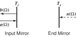
Figure 2: Filter cavity with input $a(\Omega)$, output $b(\Omega)$ and noise $n(\Omega)$ field operators. We indicate with $T_{i}$ and $T_{e}$ the power transmissivity of the input and end mirrors, respectively.

III.2 KLMTV filters with low loss

Following KLMTV, we model losses in a filter cavity by assuming that the end mirror has a non-vanishing power transmissivity $T_{e}$, and a power reflectivity of $R_{e}=1-T_{e}$. Denoting the front-mirror power transmissivity and reflectivity by $T_{i}$ and $R_{i}$ ($T_{i}+R_{i}=1$), the filter input-output relation to first order in $T_{e}/T_{i}$ reads:

$$\left(\begin{array}[]{c}b_{1}^{\rm out}\\ b_{2}^{\rm out}\end{array}\right)=\sqrt{1-\mathcal{E}}\,\mathbf{R}(\zeta)\,\left(\begin{array}[]{c}b_{1}^{\rm in}\\ b_{2}^{\rm in}\end{array}\right)+\sqrt{\mathcal{E}}\,\left(\begin{array}[]{c}n_{1}^{\rm filter}\\ n_{2}^{\rm filter}\end{array}\right)\,,$$ (47)

where the rotation $\mathbf{R}(\zeta)$ is the same as in the lossless case, $n_{1,2}^{\rm filter}$ are vacuum quadrature fields leaking in from the end mirror, and the loss factor $\mathcal{E}$ is given by

$$\mathcal{E}=\frac{1}{2}\sum_{s=+,-}\mathcal{E}_{s}\,,$$ (48)

with

$$\mathcal{E}_{\pm}=\frac{2\,T_{e}}{T_{i}}\,\frac{2}{1+(\pm\Omega-\omega_{f})^{2}/\gamma_{f}^{2}}\,,\qquad\Omega_{\mathrm{res}}=\omega_{f}-i\gamma_{f}\,.$$ (49)

Here $\omega_{f}$, $\gamma_{f}$, $L_{f}$ are the resonant frequency, bandwidth and length of the filter, respectively. The bandwidth $\gamma_{f}$ is related to $T_{i}$ and $L_{f}$ by

$$\gamma_{f}=\frac{T_{i}\,c}{4L_{f}}\,.$$ (50)

[The optical-filter parameters are summarized in Table 2.] For a sequence of multiple filters, the rotation angles $\zeta$ and loss factors $\mathcal{E}$ of each filter add up to give the total rotation angle and loss factor. In this way, the total rotation angle will be identical to the ideal value, while the total loss factor will be

$$\mathcal{E}=\frac{1}{2}\sum_{s=+,-\atop J=\rm filters}\mathcal{E}_{s}^{J}\,.$$ (51)

The total loss factor is frequency dependent, but never exceeds the upper limit

$$\mathcal{E}_{\rm max}=\sum_{J=\rm filters}\frac{4T_{e}^{J}}{T_{i}^{J}}\,.$$ (52)

Moreover, if the filters have eigenfrequencies well-separated from each other, that is

$$\left||\omega_{f}^{I}|-|\omega_{f}^{J}|\right|\gg\max\{\gamma_{f}^{I},\gamma_{f}^{J}\}\,,$$ (53)

and if all filters have high “quality factors,” that is

$$\omega_{f}^{J}\gg\gamma_{f}^{J}\,,$$ (54)

then, if we evaluate Eq. (51) around the resonant frequencies only one term dominates, yet away from resonances the loss factor is not very large. The total loss factor has peaks at the resonant frequencies of each filter, with peak value

$$\mathcal{E}_{\rm res}^{J}=\frac{2T_{e}^{J}}{T_{i}^{J}}\,,\quad\quad\Omega\simeq|\Omega_{\rm res}^{J}|\,.$$ (55)

and width comparable to $\gamma^{J}_{f}$.

Once a filter’s bandwidth $\gamma_{f}$ and the end-mirror transmissivity $T_{e}$ are specified, we can rewrite the peak value of the total loss factor (near this filter’s resonant frequency) as

$$\mathcal{E}_{\rm res}^{J}=\frac{T_{e}^{J}c}{2\gamma_{f}^{J}L_{f}}\,,\quad\quad\Omega\simeq|\Omega_{\rm res}^{J}|\,.$$ (56)

Thus, the shorter the cavity, the lower the front-mirror transmissivity and the larger the loss factor. As an order-of-magnitude estimate, we show in Table 3 the values of $\mathcal{E}_{\rm res}$ evaluated for typical filter lengths ($4000\,$m, $400\,$m, and $30\,$m) and bandwidths $\gamma_{f}$ ($2\pi\times 100$ Hz and $2\pi\times 25\,$Hz), having assumed $T_{e}=20\,$ppm Whitcomb .

$L_{f}$	$\gamma_{f}/(2\pi)$	$\mathcal{E}_{\rm res}$
4000 m	100 Hz	0.0012
	25 Hz	0.0048
400 m	100 Hz	0.012
	25 Hz	0.048
30 m	100 Hz	0.16
	25 Hz	0.64

Table 3: Peak values of the filter power-loss factor, $\mathcal{E}_{\rm res}$ [Eq. (56)], for various filter lengths and bandwidths, assuming an end-mirror transmissivity of 20 ppm.

III.3 KLMTV filters with significant loss

As we can see from Table 3, when the filters are short, e.g., on the order of 30 m, the energy loss factor can become quite large, and the leading-order calculation used in Sec. III.2 can no longer be trusted. Instead, here we give the exact filter input-output relation. By denoting with $a(\Omega)$, $b(\Omega)$ and $n(\Omega)$ the (Fourier domain) annihilation operators of the input, output and noise fields at frequency $\omega_{0}+\Omega$, we have [see Fig. 2]:

$$b(\Omega) = \frac{\sqrt{R_{e}}\,e^{2i(\Omega-\omega_{f})L_{f}/c}-\sqrt{R_{i}}}{1-\sqrt{R_{i}R_{e}}\,e^{2i(\Omega-\omega_{f})L_{f}/c}}\,a(\Omega)$$ (57)

$$+ \frac{\sqrt{T_{i}T_{e}}\,e^{i(\Omega-\omega_{f})L_{f}/c}}{1-\sqrt{R_{i}R_{e}}\,e^{2i(\Omega-\omega_{f})L_{f}/c}}\,n(\Omega)\,.$$

Here $\omega_{0}+\omega_{f}$ is the resonant frequency of the filter cavity (the one nearest $\omega_{0}$). The quadrature input-output relation can be obtained from Eq. (57) by using, e.g., Eqs. (A8) and (A9) of Ref. BC5 . Namely, the relation

$$b(\pm\Omega)=f_{\pm}(\Omega)\,a(\pm\Omega)$$ (58)

valid for annihilation operators is equivalent to the relation

$$\left(\begin{array}[]{c}b_{1}\\ b_{2}\end{array}\right)=\frac{1}{2}\left(\begin{array}[]{cc}(f_{+}+f_{-}^{*})&i(f_{+}-f_{-}^{*})\\ -i(f_{+}-f_{-}^{*})&(f_{+}+f_{-}^{*})\end{array}\right)\left(\begin{array}[]{c}a_{1}\\ a_{2}\end{array}\right)\,,$$ (59)

valid for quadrature fields $a_{1,2}$ and $b_{1,2}$. [Note the typo in the (2,1) component of Eq. (A9) of Ref. BC5 .]

Again, we can apply the short-filter approximation, $\Omega L/c$, $\omega_{f}L/c$, $\gamma_{f}L/c\ll 1$, $T_{e}\stackrel{{\scriptstyle<}}{{{}_{\sim}}}T_{i}$, and obtain simpler formulas:

$$b=\frac{1-\alpha_{f}+i\displaystyle\frac{\Omega-\omega_{f}}{\gamma_{f}}}{1+\alpha_{f}-i\displaystyle\frac{\Omega-\omega_{f}}{\gamma_{f}}}\,a+\frac{2\sqrt{\alpha_{f}}}{1+\alpha_{f}-i\displaystyle\frac{\Omega-\omega_{f}}{\gamma_{f}}}\,n\,,$$ (60)

where $\alpha_{f}=T_{e}/T_{i}$. By converting into the quadrature representation we have:

$$\left(\begin{array}[]{c}b_{1}\\ b_{2}\end{array}\right)=\frac{(\mathcal{R}+i\alpha_{f}\,\Lambda)\left(\begin{array}[]{c}a_{1}\\ a_{2}\end{array}\right)+2\sqrt{\alpha_{f}}\,\mathcal{N}\left(\begin{array}[]{c}n_{1}\\ n_{2}\end{array}\right)}{\left(1+\alpha_{f}-\displaystyle i\frac{\Omega+\omega_{f}}{\gamma_{f}}\right)\left(1+\alpha_{f}-\displaystyle i\frac{\Omega-\omega_{f}}{\gamma_{f}}\right)}\,,$$ (61)

where $n_{1,2}$ are quadratures of the field $n$,

$$\mathcal{R}=\left(\begin{array}[]{cc}1-\alpha_{f}^{2}+\frac{\Omega^{2}-\omega_{f}^{2}}{\gamma_{f}^{2}}&\frac{2\omega_{f}}{\gamma_{f}}\\ -\frac{2\omega_{f}}{\gamma_{f}}&1-\alpha_{f}^{2}+\frac{\Omega^{2}-\omega_{f}^{2}}{\gamma_{f}^{2}}\end{array}\right)\,,$$ (62)

$$\Lambda=\frac{2\Omega}{\gamma}\,\mathbf{I}\,,$$ (63)

and

$$\mathcal{N}=\left(\begin{array}[]{cc}1+\alpha_{f}-i\frac{\Omega}{\gamma_{f}}&\frac{\omega_{f}}{\gamma_{f}}\\ -\frac{\omega_{f}}{\gamma_{f}}&1+\alpha_{f}-i\frac{\Omega}{\gamma_{f}}\end{array}\right)\,.$$ (64)

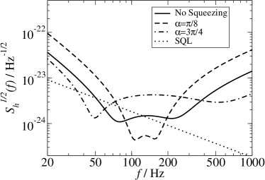
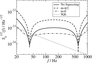
Figure 3: Noise curves of SR interferometers with frequency independent input squeezing and homodyne readout. In the left panel, we show the broadband configuration: $\lambda=2\pi\times 234.07\,{\rm Hz}$, $\epsilon=2\pi\times 70.36\,{\rm Hz}$, $\zeta=-0.8037$, with no input squeezing ($r=0$, $\alpha=0$) (continuous curve), with $e^{2r}=10$, $\alpha=\pi/8$ (dashed curve) and with $e^{2r}=10$, $\alpha=3\pi/4$ (dash-dot curve). In the right panel, we plot the narrowband configuration: $\lambda=2\pi\times 600\,{\rm Hz}$, $\epsilon=2\pi\times 25\,{\rm Hz}$, $\zeta=\pi/2$, with no input squeezing ($r=0$, $\alpha=0$) (continuous curve), with $e^{2r}=10$, $\alpha=\pi/2$ (dashed curve) and with $e^{2r}=10$, $\alpha=0$ (dash-dot curve). In both configurations we fix $I_{c}=840\,$kW and $m=40\,$kg and show the SQL curve (dotted line).

IV Squeezed-input and variational-output signal recycled interferometers

IV.1 Input-output relation and noise spectral density

As discussed by KLMTV, a GW interferometer with squeezed vacuum state $|S(r,\alpha)\rangle$ fed into its input port can be described by applying the following unitary transformation,

$$\left(\begin{array}[]{c}a_{1}\\ a_{2}\end{array}\right) \rightarrow \mathbf{R}(\alpha)\mathbf{S}(r)\left(\begin{array}[]{c}\tilde{a}_{1}\\ \tilde{a}_{2}\end{array}\right)\,,$$ (69)

$$|S(r,\alpha)_{a}\rangle \rightarrow |0_{\tilde{a}}\rangle\,,$$ (70)

in which the quadrature operators undergo a linear transformation, while the quantum state is transformed back to the vacuum state. [Note that $\langle 0_{\tilde{a}}|\tilde{a}_{i}\,\tilde{a}_{j}^{\dagger}|0_{\tilde{a}}\rangle=2\pi\,\delta_{ij}\,\delta(\Omega-\Omega^{\prime})$.] Equation (69) suggests that, in practice, the squeeze angle $\alpha$ of the squeezed vacuum injected into the input port can be obtained by a quadrature-rotating optical element, e.g., a KLMTV filter, placed between the squeezer and the interferometer.

Once the unitary transformation is applied, the input-output relation of the interferometer can be written similarly to Eq. (1) as

$$\left(\begin{array}[]{c}b_{1}\\ b_{2}\end{array}\right)=\frac{1}{M}\left[\left(\begin{array}[]{cc}C^{\alpha}_{11}&C_{12}^{\alpha}\\ C_{21}^{\alpha}&C_{22}^{\alpha}\end{array}\right)\left(\begin{array}[]{r}e^{-r}\tilde{a}_{1}\\ e^{+r}\tilde{a}_{2}\end{array}\right)+\left(\begin{array}[]{c}D_{1}\\ D_{2}\end{array}\right)\frac{h}{h_{\rm SQL}}\right]\,,$$ (71)

where

$$\left(\begin{array}[]{cc}C^{\alpha}_{11}&C_{12}^{\alpha}\\ C_{21}^{\alpha}&C_{22}^{\alpha}\end{array}\right)\equiv\left(\begin{array}[]{cc}C_{11}\,\cos\alpha+C_{12}\,\sin\alpha&C_{12}\,\cos\alpha-C_{11}\,\sin\alpha\\ C_{21}\,\cos\alpha+C_{22}\,\sin\alpha&C_{22}\,\cos\alpha-C_{21}\,\sin\alpha\end{array}\right)\,.$$ (72)

The quadrature $\tilde{a}_{1}$ is generally called the “squeezed quadrature” because it enters Eq. (71) multiplied by $e^{-r}$, while $\tilde{a}_{2}$ is called the “stretched quadrature” because it is multiplied by $e^{+r}$. If the output quadrature $b_{\zeta}=b_{1}\,\sin\zeta+b_{2}\,\cos\zeta$ is measured, the noise spectral density is

$$S_{h}=\frac{e^{-2r}\left(C^{\alpha}_{11}\,\sin\zeta+C^{\alpha}_{21}\,\cos\zeta\right)^{2}+e^{2r}\left(C^{\alpha}_{12}\,\sin\zeta+C^{\alpha}_{22}\,\cos\zeta\right)^{2}}{\left|D_{1}\,\sin\zeta+D_{2}\,\cos\zeta\right|^{2}}\,h_{\rm SQL}^{2}\,,$$ (73)

which in terms of the (ponderomotive) squeeze factor $q$, intrinsic rotation angle $\varphi$, maximal-signal quadrature $\zeta_{\rm max}$ reads:

$$S_{h}=|M|^{2}\,\frac{e^{-2r}\,\left[\cosh q\,\cos(\alpha+\zeta-2\varphi)-\sinh q\,\cos(\alpha-\zeta)\right]^{2}+e^{2r}\,\left[\cosh q\,\sin(\alpha+\zeta-2\varphi)-\sinh q\,\sin(\alpha-\zeta)\right]^{2}}{4\epsilon\iota_{c}\Omega^{2}\left[S_{0}+S_{1}\cos 2(\zeta-\zeta_{\rm max})\right]}\,h_{\rm SQL}^{2}\,.$$ (74)

In Eqs. (73) and (74), the spectral density $S_{h}$ contains a term proportional to $e^{-2r}$, as well as one proportional to $e^{2r}$. We can take advantage of squeezed vacuum only if $b_{\zeta}$ contains very little (preferably none) of the stretched quadrature $\tilde{a}_{2}$.

In Fig. 3 we plot some examples of noise spectral densities with frequency independent input squeezing (constant $\alpha$) and readout (constant $\zeta$). In this case, squeezing can improve the sensitiviy at some frequencies, but at the price of deteriorating the sensitivity at other frequencies. However, as investigated by Corbitt, Mavalvala and Whitcomb CM ; CMW , without introducing FD input-output techniques, it is still possible to take advantage of input squeezing, by choosing carefully the SR parameters $(\lambda,\epsilon,\iota_{c})$, and/or by filtering out the squeezed vacuum in the frequency region where the stretched quadrature increases the noise. On the other hand, if, for a substantially detuned configuration, we would like to obtain a large noise-suppression factor over the entire frequency band, FD input-output techniques should be used.

IV.2 Cancellation of the stretched quadrature and sub-optimal schemes

In order that $S_{h}$ in Eq. (73) has only the term proportional to $e^{-2r}$, we have to impose

$$C_{12}^{\alpha}\sin\zeta+C_{22}^{\alpha}\cos\zeta=0\,,$$ (75)

or, more symmetrically in $\alpha$ and $\zeta$,

$$\left(\begin{array}[]{cc}\sin\zeta&\cos\zeta\end{array}\right)\left(\begin{array}[]{cc}C_{11}&C_{12}\\ C_{21}&C_{22}\end{array}\right)\left(\begin{array}[]{r}-\sin\alpha\\ \cos\alpha\end{array}\right)=0\,.$$ (76)

It is interesting to note that Eq. (76) does not depend on $r$. This happens because the way $e^{-r}\,\tilde{a}_{1}$ and $e^{r}\,\tilde{a}_{2}$ are mapped into $b_{\zeta}$ [see Eq. (71)] depends only on $\alpha$, $C_{ij}$, and $\zeta$, but not on $r$.

Equation (76) can be satisfied in many ways. However, since $C_{ij}$ are frequency dependent, either $\alpha$ or $\zeta$, or both, will have to be frequency dependent. Given such a pair of $(\alpha(\Omega),\zeta(\Omega))$, the noise spectrum can be obtained by inserting them into Eq. (73), obtaining

$$S_{h}=\frac{e^{-2r}\left[C_{11}^{\alpha(\Omega)}\sin\zeta(\Omega)+C_{21}^{\alpha(\Omega)}\cos\zeta(\Omega)\right]^{2}+e^{2r}\left[C_{12}^{\alpha(\Omega)}\sin\zeta(\Omega)+C_{22}^{\alpha(\Omega)}\cos\zeta(\Omega)\right]^{2}}{|D_{1}\sin\zeta(\Omega)+D_{2}\cos\zeta(\Omega)|^{2}}h_{\rm SQL}^{2}\,,$$ (77)

with the second term in the numerator vanishing once Eq. (76) is imposed. As a consequence, we can also write

$$S_{h} = e^{-2r}\frac{\left[C_{11}^{\alpha(\Omega)}\sin\zeta(\Omega)+C_{21}^{\alpha(\Omega)}\cos\zeta(\Omega)\right]^{2}+\left[C_{12}^{\alpha(\Omega)}\sin\zeta(\Omega)+C_{22}^{\alpha(\Omega)}\cos\zeta(\Omega)\right]^{2}}{|D_{1}\sin\zeta(\Omega)+D_{2}\cos\zeta(\Omega)|^{2}}h_{\rm SQL}^{2}$$ (78)

$$= e^{-2r}\frac{\left[C_{11}\sin\zeta(\Omega)+C_{21}\cos\zeta(\Omega)\right]^{2}+\left[C_{12}\sin\zeta(\Omega)+C_{22}\cos\zeta(\Omega)\right]^{2}}{|D_{1}\sin\zeta(\Omega)+D_{2}\cos\zeta(\Omega)|^{2}}h_{\rm SQL}^{2}\,.$$

The first equality in Eq. (78) says that the noise spectrum of an input-output scheme [as specified by ($\alpha(\Omega)$,$\zeta(\Omega)$)] with an input squeeze factor $r$ scales as $e^{-2r}$; the second equality in Eq. (78) must hold since for ordinary vacuum a rotation of the input quadratures leaves the system invariant. The spectral density, as given by Eq. (78), is $e^{-2r}$ times that of a (non-squeezed) FD readout scheme with homodyne phase $\zeta(\Omega)$. Clearly, an additional optimization in $\zeta$ will give the fully optimal input-output scheme. However, we postpone the discussion of the fully optimal scheme till Sec. IV.4 and investigate first the sub-optimal schemes, which have $(\alpha(\Omega),\zeta(\Omega))$ satisfying Eq. (76) but do not necessarily have the optimal $\zeta(\Omega)$ required by the minimization of (78). These schemes all provide a global noise suppression by the factor $e^{-2r}$.

The (two) simplest solutions to Eq. (76) can be obtained by imposing $\zeta$ (or $\alpha$) to be frequency independent and solving Eq. (76) for $\alpha$ (or $\zeta$). This means that KLMTV filters are placed either in the input port or in the output port, but not in both places.

The first simple solution has been studied by Harms et al. Harms03 , who proposed to inject squeezed vacuum with FD squeeze angle into SR interferometers. Imposing a frequency independent $\zeta$, they obtained

$$\tan\alpha_{\rm subopt}(\Omega)=\frac{C_{22}\,\cos\zeta+C_{12}\,\sin\zeta}{C_{21}\,\cos\zeta+C_{11}\,\sin\zeta}\,.$$ (79)

Remarkably, the required $\alpha_{\rm subopt}$ in Eq. (79) is of the form (43), thus realizable by KLMTV filters. In our notations, the characteristic equation for the filters is

$$\Omega^{2}(\Omega+\lambda-i\epsilon)(\Omega-\lambda+i\epsilon)+\left[\lambda-2ie^{-i\zeta}\epsilon\cos\zeta\right]\,\iota_{c}=0\,,$$ (80)

while the constant rotation following the filters should be

$$\theta=\pi/2-\zeta\,.$$ (81)

[See Eqs. (44) and (45).] Note that, without making the short-arm and short-filter approximations, both Eqs. (79) and (43) would have been much more complicated, making the identification of filter parameters much less straightforward (or even impossible).

In this paper, we explore the second simple solution. We assume a frequency independent $\alpha$ and requires the FD detection phase

$$\tan\zeta_{\rm subopt}(\Omega)=-\frac{C_{22}\,\cos\alpha-C_{21}\,\sin\alpha}{C_{12}\,\cos\alpha-C_{11}\,\sin\alpha}\,.$$ (82)

This detection phase is also of the form (43) and realizable by KLMTV filters, with characteristic equation

$$\Omega^{2}(\Omega+\lambda-i\epsilon)(\Omega-\lambda+i\epsilon)+\left[\lambda+2e^{-i\alpha}\epsilon\sin\alpha\right]\iota_{c}=0\,,$$ (83)

and a subsequent frequency independent rotation

$$\theta=3\pi/2-\alpha\,.$$ (84)

Henceforth, we shall call this scheme the BC scheme. The noise spectral density of the BC scheme can be obtained by inserting Eq. (82) into Eq. (78); the result is

$$S_{h}=\frac{e^{-2r}|M|^{2}h_{\rm SQL}^{2}}{4\epsilon\iota_{c}\Omega^{2}|\lambda\cos\alpha+(\epsilon-i\Omega)\sin\alpha|^{2}}\,.$$ (85)

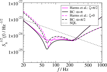
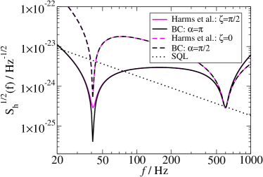
Figure 4: Equivalence of the Harms et al. and BC schemes at high frequencies. We assume $I_{c}=840\,$kW, $m=40\,$kg and $e^{2r}=10$. In the left panel, we plot the broadband configurations with $\lambda=2\pi\times 234.07\,{\rm Hz}$, $\epsilon=2\pi\times 70.36\,{\rm Hz}$, while in the right panel we show narrowband configurations with $\lambda=2\pi\times 600\,{\rm Hz}$ and $\epsilon=2\pi\times 25\,$Hz. In both panels, BC schemes with $\alpha=\pi$ and $\pi/2$ are shown in dark continuous and dark dashed curves, respectively, while Harms et al. schemes with $\zeta=\pi/2$ and $\zeta=0$ are shown in light continuous and light dashed curves. Noise curves from the two schemes, which are related by $\alpha=\zeta+\pi/2$, do agree quite well for frequencies higher than $200\,$Hz in the broadband configuration (left panel), and at almost all frequencies in the narrowband configuration (right panel). Note that at high frequencies $q$ is significantly lower in the narrowband configuration, see left panel of Fig. 3.

Additional insight into these sub-optimal schemes can be obtained by decomposing the input-output $\tilde{a}$-$b$ relation into a product of rotation and squeezing operators [see Eqs. (23), (69) and (71)]:

$$\Delta b_{\zeta}=\underbrace{\Bigg{[}\left(\begin{array}[]{cc}0&1\end{array}\right)\mathbf{R}(\zeta)\Bigg{]}}_{\mbox{readout}}\underbrace{\Bigg{[}\mathbf{R}(\pi/2-\varphi)\mathbf{S}(q)\mathbf{R}(-\varphi)\Bigg{]}}_{\mbox{interferometer}}\underbrace{\Bigg{[}\mathbf{R}(\alpha)\mathbf{S}(r)\left(\begin{array}[]{c}\tilde{a}_{1}\\ \tilde{a}_{2}\end{array}\right)\Bigg{]}}_{\mbox{input}}\,,$$ (86)

Here $\Delta b_{\zeta}$ is the fluctuating (noise) part of $b_{\zeta}$. Equation (76) can then be put into the following form:

$$\underbrace{\left(\begin{array}[]{cc}0&1\end{array}\right)\mathbf{R}(\zeta)}_{\rm readout}\,\underbrace{\mathbf{R}(\pi/2-\varphi)\,\mathbf{S}(q)\mathbf{R}(-\varphi)}_{\rm interferometer}\,\underbrace{\mathbf{R}(\alpha)\left(\begin{array}[]{c}0\\ 1\end{array}\right)}_{\rm input}=0\,.$$ (87)

In the Harms et al. scheme, the input quadratures are rotated (with FD angle $\alpha$), before entering the interferometer, in such a way that, after being rotated again and ponderomotively squeezed by the interferometer opto-mechanical dynamics, the squeezed quadrature is mapped into a frequency independent output quadrature, which is detected. In the BC scheme a frequency independent squeezed state enters the interferometer. Due to rotation and ponderomotive squeezing inside the interferometer, the squeezed quadrature is mapped into a FD output quadrature. We then apply a rotation to the field emerging from the interferometer to counteract this effect and bring the (image of the) input squeeze quadrature back to a frequency independent quadrature and detect it.

Finally, another interesting sub-optimal scheme can be obtained by imposing $\zeta=\alpha=-\varphi$. In this case the noise part of the output quadrature field (86) is

$$\left(\begin{array}[]{cc}0&1\end{array}\right)\mathbf{R}(\pi/2)\,\mathbf{S}(q)\,\mathbf{S}(r)\left(\begin{array}[]{c}\tilde{a}_{1}\\ \tilde{a}_{2}\end{array}\right)=e^{-(r+q)}\tilde{a}_{1}$$ (88)

which gives the lowest amount of noise (but does not guarantee a maximal signal content). Unfortunately, from Eq. (26) we see that $\tan\zeta=-\tan\varphi$ is not of the form (43), and thus not realizable by KLMTV filters.

IV.3 Sub-optimal schemes using $q\mbox{--}\varphi$ parametrization: the low-power limit

If the ponderomotive squeezing factor $q$ is small, the fully optimal input-output scheme can be solved easily using the various quadrature-rotation angles. As seen in Sec. II, a small $q$ can either arise from a low optical power, or from considering high frequencies ($f\stackrel{{\scriptstyle>}}{{{}_{\sim}}}300\,{\rm Hz}$ for Advanced LIGO power), see Eq. (26). However, we shall still refer to this as the low-power limit. In this case, the output noise is proportional to

$$\left(\begin{array}[]{cc}0&1\end{array}\right)\mathbf{R}(\zeta+\pi/2-2\,\varphi_{\mbox{\scriptsize low-power}}+\alpha)\,\mathbf{S}(r)\left(\begin{array}[]{c}\tilde{a}_{1}\\ \tilde{a}_{2}\end{array}\right)\,,$$ (89)

and the minimal noise is obtained whenever

$$\zeta+\alpha=2\,\varphi_{\mbox{\scriptsize low-power}}\,.$$ (90)

By setting $\zeta$ equal to the maximal-signal quadrature [see Eq. (40)],

$$\zeta_{\rm max}=-\frac{\pi}{4}+\varphi_{\mbox{\scriptsize low-power}}\,,$$ (91)

we find the fully optimal readout scheme:

$$(\zeta,\alpha)_{\rm opt}=\left(-\frac{\pi}{4}+\varphi_{\mbox{\scriptsize low-power}},\frac{\pi}{4}+\varphi_{\mbox{\scriptsize low-power}}\right)\,.$$ (92)

Simple as it looks, this fully optimal scheme is not realizable by KLMTV filters because $\tan\zeta_{\rm opt}$ and $\tan\alpha_{\rm opt}$ given by Eq. (92) are not of the form (43).

We now compare the Harms et al. (H) and BC schemes in the small-$q$ regime. They can be written in terms of $(\zeta,\alpha)$ as

$$(\zeta,\alpha)_{\rm H} = (\zeta,2\,\varphi_{\mbox{\scriptsize low-power}}-\zeta)\,,$$

$$(\zeta,\alpha)_{\rm BC} = (2\,\varphi_{\mbox{\scriptsize low-power}}-\alpha,\alpha)\,.$$ (93)

The two schemes give the same noise output part $e^{-r}\,\tilde{a}_{1}$ [see Eq. (89)], while for the signal power they yield [see Eqs. (36)–(38)]

$$s_{\scriptscriptstyle H} = S_{0}+S_{1}\cos\left[2(\zeta-\zeta_{\rm max})\right]$$ (94)

$$= S_{0}+S_{1}\cos(2\,\zeta+\pi/2-2\,\varphi_{\mbox{\scriptsize low-power}})\,,$$

and

$$s_{\scriptscriptstyle BC} = S_{0}+S_{1}\cos\left[2(\zeta-\zeta_{\rm max})\right]$$ (95)

$$= S_{0}+S_{1}\cos(-2\,\alpha+\pi/2+2\,\varphi_{\mbox{\scriptsize low-power}})$$

$$= S_{0}+S_{1}\cos(2\,\alpha-\pi/2-2\,\varphi_{\mbox{\scriptsize low-power}})\,.$$

This means, the two sub-optimal schemes have the same ideal performance in the low-power regime and we can map one into the other by setting $\alpha\leftrightarrow\zeta+\pi/2$.

This equivalence can be understood more intuitively if we compare the dependence of the various readout quadratures (i.e., maximum-signal, Harms et al., and BC) on $\varphi_{\mbox{\scriptsize low-power}}$.

The maximal-signal quadrature $\zeta_{\rm max}$ rotates as ${\rm const}+\varphi_{\mbox{\scriptsize low-power}}$. In the Harms et al. scheme, the detected quadrature is constant, and therefore lags the maximal-signal quadrature by ${\rm const}+\varphi_{\mbox{\scriptsize low-power}}$. In the BC scheme, the detected quadrature rotates as $\zeta={\rm const}+2\varphi_{\mbox{\scriptsize low-power}}$, which advances the optimal quadrature by ${\rm const}+\varphi_{\mbox{\scriptsize low-power}}$. In this way, if one adjusts the constants (by adjusting $\zeta$ in the Harms et al. scheme and $\alpha$ in the BC scheme), the detected quadratures in the two schemes can be made to lie symmetrically on each side of the maximal-signal quadrature. Since the detected signal power depends only on $\cos\left[2(\zeta-\zeta_{\rm max})\right]$ [see Eq. (36)], which is an even function of $(\zeta-\zeta_{\rm max})$, the two schemes must detect the same signal power and hence have the same sensitivity.

In Fig. 4, we give examples of the BC and Harms et al. noise curves for two SR interferometers, a broadband configuration (with $\lambda=2\pi\times 234.07\,{\rm Hz}$, $\epsilon=2\pi\times 70.36\,{\rm Hz}$) and a narrowband one (with $\lambda=2\pi\times 600\,{\rm Hz}$ and $\epsilon=2\pi\times 25\,$Hz). For both interferometers, we use $I_{c}=840\,$kW, $m=40\,$kg. Although the optical power used here is not low by any practical standards, the two schemes for the broadband configuration already agree quite well, under the correspondence $\alpha\leftrightarrow\zeta+\pi/2$, for frequencies above $\sim$200 Hz. The two schemes are equivalent for the narrowband configuration for almost all frequencies. The better agreement in the narrowband configuration can be understood easily by realizing that ponderomotive squeezing is weaker in this case, as shown in the left panel of Fig. 3.

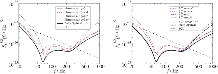
Figure 5: Approaching the fully optimal input-output scheme by taking the envelope of Harms et al. and BC noise curves. We fix $I_{c}=840\,$kW and $m=40\,$kg, and $\lambda=2\pi\times 234.07\,{\rm Hz}$, $\epsilon=2\pi\times 70.36\,{\rm Hz}$, and assume $e^{2r}=10$. In the left panel, we plot the noise curves of Harms et al. schemes, with frequency independent readout phase $\zeta=$ 0 (light short dash), $\pi/4$ (light long dash), $\pi/2$ (light dot dash) and $3\pi/4$ (light dot), and FD input squeeze angle given by Eq. (79). These curves cross each other near both the optical resonance and the optical-spring resonance. The fully optimal curve (dark continuous) is obtained by taking the lower envelope of the entire family of these curves. In the right panel, we plot the BC curves, with frequency independent input squeeze angle $\alpha=-\pi/2$ (light short dash), $-\pi/4$ (light long dash), $0$ (light dot dash) and $\pi/4$ (light dot), and FD readout phase given by Eq. (82). The lower envelope of these curves also gives the fully optimal noise curve (dark continuous, indentical to the one shown in left panel). The fact that these curves do not cross each other at low frequencies suggests that one member of this family is fully optimal in this band. Indeed, the BC curve optimized for $\Omega=0$ [dark dashed curve, with $\alpha=\arctan\epsilon/\lambda$, see Eq. (100)] does agree very well with the fully optimal curve for frequencies lower than $\sim 200$ Hz. In both panels we also show the SQL line.

IV.4 The fully optimal scheme and the BC scheme at low frequencies

In this section, we consider the fully optimal scheme. Analytical formulas of the fully optimal detection quadrature has been obtained by Harms et al., but we provide an alternative approach, yielding results in simpler form and more related to the BC scheme.

It is straightforward to show that (as also done by Harms et al. and reviewed in Appendix A), fixing $\zeta$ and $r$, the $\alpha$ obtained from Eq. (79) gives the (constrained) minimum noise. On the contrary, fixing $\alpha$ and $r$, the readout quadrature $\zeta$ obtained from Eq. (82) does not give the constrained minimum. Instead, minimizing $S_{h}$ [Eq. (73)] over $\zeta$ (with $\alpha$ fixed) requires a rather complicated readout phase, determined by one of the two roots of

$${\cal F}_{2}\tan^{2}\zeta+{\cal F}_{1}\,\tan\zeta+{\cal F}_{0}=0\,,$$ (96)

where

$${\cal F}_{2} = \left[(C^{\alpha,-r}_{11})^{2}+(C^{\alpha,r}_{12})^{2}\right]\,\Re(D_{1}^{*}D_{2})-\left(C^{\alpha,-r}_{11}\,C^{\alpha,-r}_{21}+C^{\alpha,r}_{12}\,C^{\alpha,r}_{22}\right)\,|D_{1}|^{2}\,,$$ (97a)

$${\cal F}_{1} = \left((C^{\alpha,-r}_{11})^{2}+(C^{\alpha,r}_{12})^{2}\right)\,|D_{2}|^{2}-\left[(C^{\alpha,-r}_{21})^{2}+(C^{\alpha,r}_{22})^{2}\right]\,|D_{1}|^{2}\,,$$ (97b)

$${\cal F}_{0} = \left(C^{\alpha,-r}_{11}\,C^{\alpha,-r}_{21}+C^{\alpha,r}_{12}\,C^{\alpha,r}_{22}\right)\,|D_{2}|^{2}-\left[(C^{\alpha,-r}_{21})^{2}+(C^{\alpha,r}_{22})^{2}\right]\,\Re(D_{1}^{*}D_{2})\,.$$ (97c)

Equations (96)–(97c), which we obtained independently BCUnpub from Harms et al., are equivalent to Eqs. (28)–(30) of Harms et al. once we set $r$ to zero in Eqs. (97a)–(97c).

As said above, the fully optimal scheme, denoted by $(\alpha_{\rm opt}(\Omega),\zeta_{\rm opt}(\Omega))$, should satisfy the sub-optimal condition (76). As a consequence, the noise spectrum of the fully optimal scheme is also given by Eq. (78), when $\zeta(\Omega)$ is replaced by $\zeta_{\rm opt}(\Omega)$. Therefore, $\zeta_{\rm opt}(\Omega)$ can be obtained by minimizing the $S_{h}$ in Eq. (78), which is given by the special case of Eqs. (96)–(97c) with $r=0$ [or Eqs. (28)–(30) of Ref. Harms03 ]; $\alpha_{\rm opt}(\Omega)$ can then be obtained from Eq. (79). It is evident from Eq. (96) that the fully optimal scheme cannot be realized by KLMTV filters, except in special cases, e.g., for conventional interferometers. As observed by Harms et al., the optimal noise spectrum can also be obtained graphically, by plotting all the noise curves with different constant values of $\zeta$, and then taking the lower envelope of all these curves, as seen in the left panel of Fig. 5 (and Fig. 4 of Ref. Harms03 ). The optimal $\zeta$ at each frequency is the one whose noise curve touches the envelope.

We now deduce the optimal scheme in another way. Again, since $(\alpha_{\rm opt}(\Omega),\zeta_{\rm opt}(\Omega))$ satisfy Eq. (76), the fully optimal noise spectral density can also be obtained by taking the minimum among all BC noise spectral densities with all possible $\alpha$ — the minimum is achieved automatically in $\alpha_{\rm opt}(\Omega)$, and for $\zeta_{\rm opt}(\Omega)$ it is given by Eq. (82). Similarly, this can be done graphically by taking the lower envelope of BC noise curves with all possible $\alpha$, as shown in the right panel of Fig. 5. From the plot, it is interesting to observe that, there are no crossings between different BC noise curves at low frequencies (differently from the Harms et al. curves in the left panel), suggesting that one BC curve might be nearly fully optimal at these frequencies!

More quantitatively, since the BC noise spectrum (85) has a much simpler dependence on $\alpha$ (than the dependence of the Harms et al. noise spectrum on $\zeta$), it is much simpler to obtain the optimal input squeeze angle $\alpha_{\rm opt}$ from this approach [than to obtain $\zeta_{\rm opt}$ from the approach starting with the Harms et al. noise spectrum, see Eqs. (96)–(97c)]:

$$\tan 2\alpha_{\rm opt}=\frac{2\lambda\epsilon}{\lambda^{2}-\epsilon^{2}-\Omega^{2}}\,,$$ (98)

and

$$S_{h}^{\rm opt}=\frac{e^{-2r}|M|^{2}h_{\rm SQL}^{2}}{\displaystyle 2\,\epsilon\,\iota_{c}\,\Omega^{2}(\lambda^{2}+\epsilon^{2}+\Omega^{2})\left[1+\sqrt{1-\left(\frac{2\lambda\Omega}{\lambda^{2}+\epsilon^{2}+\Omega^{2}}\right)^{2}}\right]}\,.$$ (99)

These simple explicit expressions of $S_{h}^{\rm opt}$ and $\alpha_{\rm opt}(\Omega)$ have not been previously obtained. The optimal readout phase $\zeta_{\rm opt}$ can be obtained from Eq. (82). From Eq. (98), we can see that the fully optimal scheme cannot be achieved by KLMTV filters. The only exception is when $\lambda=0$ (i.e., for a conventional interferometer). In this case we have $\alpha_{\rm opt}=0$, and the $\zeta_{\rm opt}(\Omega)$ is given by Eq. (82) and it is reliazable by KLMTV filters. This is exactly the KLMTV squeezed-variational scheme.

Although the form of $\alpha_{\rm opt}$ is not achievable by KLMTV filters, we note that, at low frequencies (lower than the optical resonant frequency), the variation in $\alpha_{\rm opt}$ is mild. In fact, by setting in the BC scheme

$$\alpha=\alpha_{\rm opt}(\Omega=0)=\arctan\left(\frac{\epsilon}{\lambda}\right)\,,$$ (100)

we obtain ,

$$S_{h}^{\rm BC\,\,low\mbox{-}freq}$$ (101)

$$= \frac{e^{-2r}|M|^{2}h_{\rm SQL}^{2}}{\displaystyle 2\,\epsilon\,\iota_{c}\,\Omega^{2}\left[2(\lambda^{2}+\epsilon^{2}+\Omega^{2})-\frac{2\lambda^{2}\Omega^{2}}{\lambda^{2}+\epsilon^{2}}\right]}\,.$$

Taking the ratio between $S_{h}^{\rm BC\,\,low\mbox{-}freq}$ and $S_{h}^{\rm opt}$, and expanding in $\Omega$, we have

$$\frac{S_{h}^{\rm BC\,\,low\mbox{-}freq}}{S_{h}^{\rm opt}}=1+\left(\frac{\lambda\epsilon}{\lambda^{2}+\epsilon^{2}}\right)^{2}\left(\frac{\Omega^{2}}{\lambda^{2}+\epsilon^{2}}\right)^{2}\,.$$ (102)

The correction factor in Eq. (102) is usually small at low frequencies. For example, by maximizing over either $\epsilon$ or $\lambda$, it is easy to show that

$$\left(\frac{\lambda\epsilon}{\lambda^{2}+\epsilon^{2}}\right)^{2}\left(\frac{\Omega^{2}}{\lambda^{2}+\epsilon^{2}}\right)^{2}<\frac{27}{256}\left(\frac{\Omega}{\max\{\lambda,\epsilon\}}\right)^{4}$$ (103)

at worst. The correction in the noise spectral density cannot exceed $\sim 10\%$ (in power) for $\Omega\sim\max\{\lambda,\epsilon\}$. For substantially detuned configurations ($\lambda$ exceeding $\sim 200\,$Hz), this makes the BC scheme essentially fully optimal up to $\sim 200\,$Hz. This result is confirmed by the right panel of Fig. 5, in which $S_{h}^{\rm BC\;low\mbox{-}freq}$ is plotted (dark dashed curve) in comparison with $S_{h}^{\rm opt}$ (dark continuous curve).

Interferometer Configuration Filter I Filter II Performance Input-Output Scheme Mirror Type $e^{-2r}$ $\displaystyle\frac{\epsilon}{2\pi\,{\rm Hz}}$ $\displaystyle\frac{\lambda}{2\pi\,{\rm Hz}}$ $\alpha$ $\zeta$ $\displaystyle\frac{\Omega_{\rm res}^{\rm I}}{2\pi\,{\rm Hz}}$ $T_{i}^{\rm I}$ (ppm) $\displaystyle\frac{\Omega_{\rm res}^{\rm II}}{2\pi\,{\rm Hz}}$ $T_{i}^{\rm II}$ (ppm) SNR 300 Mpc Event Rate Improvement No Squeezing Spherical 1 70.4 234.1 $-0.804$ 5.44 $1.00$ No Filters 0.1 561.8 55.2 $1.522$ $-0.040$ 6.73 1.89 Harms et al. 0.1 $280.4$ $296.3$ FD $-0.381$ $296.0-285.4\,i$ $717$ $-59.8-23.7\,i$ $59.6$ $7.15$ ($7.81$) $2.27$ ($2.96$) BC $0.1$ $157.4$ $355.2$ $-2.090$ FD $352.0-161.0\,i$ $404$ $-59.5-12.3\,i$ $30.9$ $6.77$ ($7.84$) $1.93$ ($2.99$) No Squeezing Mexican Hat 1 $14.4$ $179.1$ $-1.010$ $9.29$ $1.00$ No Filters $0.1$ $275.3$ $101.3$ $1.395$ $-0.131$ $10.44$ $1.42$ Harms et al. $0.1$ $106.5$ $233.9$ FD $-0.518$ $227.2-115.4\,i$ $290$ $-73.2-18.0\,i$ $45.1$ $11.73$ ($15.08$) $2.01$ ($4.27$) BC $0.1$ $55.7$ $240.5$ $-2.179$ FD $230.8-61.2\,i$ $154$ $-72.7-9.8\,i$ $24.6$ $10.45$ ($15.63$) $1.42$ ($4.76$)

Table 4: Optimizations of SR interferometers with (i) no squeezing, (ii) frequency independent squeezing and homodyne detection (“no filters”) (iii) FD squeezing but frequency independent readout (the Harms et al. scheme), and (iv) frequency independent squeezing but FD readout (the BC scheme) for neutron-star–binary inspirals, with quantum noise, seismic noise and thermoelastic noise (with spherical and Mexican-Hat mirrors) included. The only optical losses included are those from the 30-m optical filters. The round-trip loss of each filter is set to be $20\,$ppm Whitcomb . Noise curves of configurations listed here are plotted in Fig. 6. For the Harms et al. and BC schemes, we also optimize the SNR when there is no optical losses, those SNRs and the corresponding event-rate improvements are quoted inside brackets.

V Applications to Advanced LIGO

In this section, we discuss the possibility of applying the above FD techniques to Advanced LIGO interferometers. As shown by KLMTV KLMTV00 , a major difficulty in making those techniques practical for advanced interferometers is the issue of optical losses. Given a certain bandwidth and mirror quality (i.e., round-trip loss in the filter cavities), the shorter the filters, the higher their optical losses (see Table 3). In fact, in order to achieve third-generation performance, optical filters in the squeezed-variational scheme will have to be $\sim$ kilometer in lengths. In Advanced LIGO, kilometer-scale filter cavities are not practical and only short filters can fit into the corner-station building. A plausible length scale is $\sim 30\,$meters; and the realistic round-trip loss is around 20 ppm Whitcomb . With such short (and lossy) filters, we shall assume most of the time that filter losses will dominate and ignore internal interferometer losses [see Sec. V in Ref. BC2 for treatment of lossy SR interferometers]. We shall only comment briefly on the effect of internal losses when discussing narrowband sources. The noise spectrum with filter losses are obtained by using the exact input-output relation of KLMTV filters (Sec. III.3).

In Secs. V.1,  V.2 and  V.3, respectively, we shall discuss the broadband configuration optimized for the detection of NS-NS binary inspiral waveforms, the narrowband configuration targeting GWs from specific accreting NS’s and the wideband configuration that can be used to observe several kind of sources. [For an exhaustive discussion and summary of GW sources for advanced interferometers see, e.g., Ref. CT .]

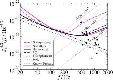
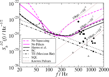
Figure 6: Noise curves optimized for NS-NS binaries, for no squeezing (“no squeezing”, light dashed curves), frequency-independent squeezing and homodyne detection (“no filters”, light continuous curves), the Harms et al. scheme (dark continuous curves) and the BC scheme (dark dashed curves). Parameters of each configuration are listed in Table 4. Quantum noise, seismic noise and thermoelastic noise of sapphire (also shown, in dash-dot curves) are included to give the total noise curves. We have used predictions for the thermoelastic noise of spherical mirrors (left panel) and that of Mexican-Hat mirrors TE (right panel). In addition, we have shown the characteristic strengths of possible GWs from LMXBs (diamond, solid circles, solid squares and open triangles) and known radio pulsars (thin dashed lines).

V.1 Broadband configuration: NS-NS binary inspiral

Inspiral waves from compact binaries (NS-NS, NS-BH or BH-BH) are among the most promising sources for Advanced LIGO. In this section, we discuss the so-called broadband configuration obtained by maximizing the signal-to-noise ratio for NS-NS inspiral waveforms, proportional to

$$\sqrt{\int_{f_{c}}^{+\infty}\frac{|\tilde{h}(f)|^{2}}{S_{h}(f)}df}\,,$$ (104)

where

$$|\tilde{h}(f)|=Af^{-7/6}\Theta(f_{\rm ISCO}-f)$$ (105)

is the frequency-domain amplitude of the leading (Newtonian) order inspiral signal in the stationary-phase approximation. The cutoff frequency is chosen to be $f_{\rm ISCO}$, the GW frequency corresponding to the Innermost Stable Circular Orbit (ISCO) of a Schwarzchild black hole with mass $2M_{\rm NS}=2\times 1.4\,M_{\odot}=2.8\,M_{\odot}$, which is equal to $1570\,$Hz. In the optimization, we have also included the seismic noise

$$\sqrt{S_{h}^{\rm seis}}=5.3\times 10^{-21}\left(\frac{10\,{\rm Hz}}{f}\right)^{9.2}\,\frac{1}{\sqrt{\rm Hz}}\,,$$ (106)

and the thermoelastic noise of sapphire mirrors with spherical surfaces, as in the baseline design,

$$\sqrt{S_{h}^{\rm TE}}=2.7\times 10^{-24}\left(\frac{100\,{\rm Hz}}{f}\right)\,\frac{1}{\sqrt{\rm Hz}}$$ (107)

as well as when the so-called Mexican-Hat mirrors are used, which are designed to reduce this noise TE ,

$$\sqrt{S_{h}^{\rm TE\,MH}}=1.1\times 10^{-24}\left(\frac{100\,{\rm Hz}}{f}\right)\,\frac{1}{\sqrt{\rm Hz}}\,.$$ (108)

In Table 4 we list the values of $\lambda$, $\epsilon$, $\alpha$ (frequency independent squeezing angle for BC scheme), $\zeta$ (frequency independent detection quadrature for Harms et al.’s scheme), obtained by optimizing the SNR of NS-NS binary inspirals at 300 Mpc, and the corresponding optimal SNR. We assume $I_{c}=840\,$kW, $m=40\,$kg, and $e^{-2r}=10$ and did the optimization for (i) non-squeezed SR interferometers, (ii) SR interferometers with frequency independent squeezing and homodyne detection (“no filters”), (iii) squeezed SR interferometers with the Harms et al. scheme (FD input squeezing + ordinary homodyne detection) and (iv) squeezed SR interferometers with the BC scheme (ordinary squeezing + FD homodyne detection). In the Table we also give the improvements in the predicted event rate with respect to non-squeezed configurations, as the cube of the improvements in SNR at a fixed distance.

As we can read from Table 4, with frequency independent squeezing (i.e., no filters), it is already possible to improve the NS-NS event rate by a significant amount, $89\%$ (spherical mirror) or $42\%$ (MH mirror). The Harms et al. scheme provides further improvement in the event rate with respect to the no-filter case, by $20\%$ (spherical mirror) or $42\%$ (MH mirror). The BC scheme, however, being more susceptible to filter optical losses, does not yield as good a performance. In order to appreciate how much the filter optical losses affect the sensitivity, we have also optimized the SNR for the FD schemes without including filter optical losses (but with thermal and seismic noises included), the results are quoted in brackets in Table 4. FD schemes without losses can outperform frequency independent squeezing significantly. For example, the ideal BC scheme can have $58\%$ (spherical mirror) or $235\%$ (MH mirror) more event rates than the no-filter case. [In this case the the BC scheme can also provide slightly higher event rates than the Harms et al. scheme, due to better sensitivity at low frequencies (but mostly still masked by the thermal noise), by $1\%$ (spherical mirror) or $11\%$ (MH mirror).]

Noise curves corresponding to the optical configurations listed in Table 4 are plotted in Fig. 6. We notice that due to optical losses the BC noise spectral densities have a peak around the optical-spring resonant frequency. The noise spectrum of the “no filters” scheme (squeezing with frequency-independent input-output optics) is comparable to the Harms et al. and BC schemes at high frequencies, but becomes worse at low frequencies. These “no-filter” curves are quite similar to the wideband noise curves proposed by Corbitt and Mavalvala CM , especially in the case of spherical mirrors.

The squeezing noise curves optimized for NS-NS binaries also have better high-frequency sensitivity than non-squeezed configurations, although they were not optimized specifically for high frequencies. From Fig. 6, we see that for frequencies higher than $\sim$500 Hz (spherical mirrors) or $\sim$300 Hz (Mexican-Hat mirrors), the squeezed configurations are $\sim 5$ – $8$ (spherical mirrors) or $\sim 3$ – $5$ (Mexican-Hat mirrors) as sensitive (in amplitude) as the non-squeezed configurations. [The Mexican-Hat mirrors produce lower thermoelastic noise, so the noise spectral densities are better optimized at low frequencies, reducing the bandwidth. This is why in this case the noise curves optimized for NS-NS binaries yield worse high-frequency sensitivity than those with spherical mirrors.]

	GW parameters			$\sqrt{S_{h_{c}}^{\mbox{\tiny 20-day}}/S_{h}(f_{\mbox{\tiny GW}})}$
	$f_{\rm GW}$	$h_{c}$	$\sqrt{S_{h_{c}}^{\mbox{\tiny 20-day}}}$	No	5 dB		10 dB
	(Hz)	$(10^{-27})$	$(10^{-24}/\sqrt{\rm Hz})$	Squeezing	Harms et al.	BC	Harms et al.	BC
GX 349$+$2	532	5.40	1.67	0.65	1.33	1.32	1.80	1.79
4U 1820$-$30	550	3.70	1.14	0.58	1.02	1.01	1.27	1.25
GX 17$+$2	588	4.70	1.45	1.48	1.52	1.51	1.65	1.63
4U 0614$+$06	654	1.30	0.40	0.19	0.35	0.34	0.44	0.43
GX 5$-$1	654	6.00	1.85	0.88	1.60	1.58	2.01	2.00
Cyg X$-$2	686	3.70	1.14	0.36	0.80	0.79	1.17	1.16
GX 340$+$0	650	3.70	1.14	0.58	1.01	1.00	1.25	1.24
Sco X$-$1	500	22.00	6.79	1.87	4.40	4.38	6.89	6.83
4U 1702$-$429	660	1.20	0.37	0.16	0.31	0.31	0.40	0.40
4U 1728$-$34	726	2.00	0.62	0.14	0.34	0.34	0.57	0.56
4U 1916$-$053	540	1.00	0.31	0.13	0.26	0.26	0.34	0.33
KS 1731$-$260	1048	1.30	0.40	0.03	0.07	0.07	0.16	0.16
Aql X$-$1	1098	1.00	0.31	0.02	0.05	0.05	0.11	0.11
MXB 1658$-$298	1134	0.30	0.09	0.01	0.01	0.01	0.03	0.03
4U 1636$-$53	1162	2.00	0.62	0.03	0.09	0.09	0.21	0.21
4U 1608$-$52	1238	1.00	0.31	0.01	0.04	0.04	0.09	0.09
SAX J1808.4$-$3658	802	0.71	0.22 (0.53)	0.03 (0.08)	0.08 (0.20)	0.08 (0.20)	0.16 (0.39)	0.16 (0.39)
XTE J1751$-$305	870	0.15	0.05	0.00	0.01	0.01	0.03	0.03
XTE J0929$-$314	370	0.25	0.08	0.01	0.03	0.03	0.06	0.05

Table 5: Frequency, characteristic amplitude $h_{c}$, and characteristic strengths ($\sqrt{S_{h_{c}}^{20\mbox{-}\rm day}}$, 20-day coherent integration with $1\%$ false alarm) of possible GWs from several known LMXBs [including Z sources (the first 8 sources), Type-I bursters (the next 8 sources) and accreting millisecond pulsars (the last 3 sources)] LB02 , and sensitivities achievable by non-squeezed, Harms et al. and BC schemes. Both 5 dB ($e^{-2r}=0.316$) and 10 dB ($e^{-2r}=0.1$) squeezing are considered. Sensitivity is measured by taking the ratio between the characteristic strength and square root of the noise spectral density at the predicted GW frequency. Bold face is used for ratios larger than unity, in which case the GW is detectable. In this Table we use the baseline assumption (a1) (i.e., $f_{s}=f_{d}$ for Z sources, and mass-quadrupole emission). To obtain the predictions for other mechanisms of GW emission and determination of the spin frequency, see Table 6. Note that $\sqrt{S_{h_{c}}}$ should convert by the same factor as $h_{c}$. For the source SAX J1808.4$-$3658 in particular, we have also shown in parenthesis values that correspond to a 4-month coherent integration.

In Fig. 6, we also plot (in light thin dashed lines) the characteristic GW strengths from known radio pulsars. Following the notation of Cutler and Thorne CT , the characteristic strength $S_{h_{c}}$ is defined as the maximum allowed noise spectral density $S_{h}(f_{\rm source})$ (at and near the source frequency $f_{\rm source}$) such that the source is detectable. Note that $S_{h_{c}}$ will in general depend on the data analysis technique and statistical criteria used, e.g., integration time, confidence level, etc.; sometimes it is also obtained by averaging over unknown source parameters, such as the spin orientation of pulsars [see App. B for more details]. Here for known radio pulsars at 10 kpc distance, with ellipticity $\epsilon=10^{-6}$, $10^{-7}$ and $10^{-8}$, we have been assuming 1$\%$ of false-alarm probability in a coherent search of $10^{7}$ s of data (coherent search for such a long time can only be done for pulsars whose sky positions and phase evolutions are known BCCS ; BC ).

From Fig. 6 we see that the NS-NS optimized noise spectra for spherical mirrors can detect known pulsars at 10 kpc with $\epsilon\stackrel{{\scriptstyle>}}{{{}_{\sim}}}10^{-7}$ if the GW frequency is higher than 500 Hz, while those for MH mirrors can detect $\epsilon\stackrel{{\scriptstyle>}}{{{}_{\sim}}}2\times 10^{-7}$ if GW frequency is higher than 300 Hz.

We have also shown in Fig. 6 the frequencies and the estimated characteristic GW strengths from LMXBs (Sco X-1 in diamond, the Z sources in solid dots, Type-I bursters in solid squares, and accreting millisecond pulsars in open triangles). We shall explain those sources in more detail in the next section and in App. B. All the squeezed-input configurations are able to detect Sco X-1 with large margins, while configurations with spherical mirrors might also be able to detect the group of six Z sources near 600 Hz.

V.2 Narrowband configuration: LMXB

Low-Mass X-ray Binaries (LMXBs) are systems formed by a neutron star and a low-mass stellar companion, from which the neutron star accrets material. Observations of LMXBs have provided evidence of a NS spin-frequency “locking” in the range $260\,{\rm Hz}<f_{s}<600\,{\rm Hz}$ (much lower than the breaking frequency of $\sim 1.5$ kHz UBC ). These systems are rather old and believed to have been spun up by accretion torque. Thus, to explain the locking it has been conjectured that accretion torque could be balanced by angular-momentum loss due to GW emission old ; B98 ; AKS . In Table V.1, we list a number of LMXBs that are promising GW sources: the first group contains the so-called Z sources, the second group the Type-I bursters, and the third group accreting millisecond pulsars (all data are taken from Refs. B98 ; UBC ; LB02 ).

The spin frequency of the NS in these LMXBs is not unambiguously determined, except for accreting millisecond pulsars, whose X-ray fluxes pulsate at their spin frequencies, i.e. $f_{P}=f_{s}$. For Type-I bursters, the spin frequency can be inferred from the millisecond oscillations in their X-ray fluxes observed after bursts ($f_{B}$) and from the kHz QPO difference frequency ($f_{d}$). However, for different sources, it has been observed that either $f_{d}=f_{B}$ or $f_{d}=f_{B}/2$, and it is not firm yet whether $f_{s}$ should be equal to $f_{B}$ or $f_{d}$. Recently, X-ray bursts have been observed SAX from the source SAX J1808.4–3658 (an accreting millisecond pulsar, with spin frequency known from $f_{s}=f_{P}$ CM98 ), and X-ray flux after the bursts is observed to oscillate at the spin frequency (i.e., $f_{B}=f_{P}=f_{s}$). Moreover, for this source the kHz QPO difference frequency is observed to be half this value: $f_{d}=f_{P}/2$. This might favor the argument that $f_{s}=f_{B}$ for all Type-I bursters, as assumed by Refs. B98 ; UBC ; LB02 and used in Table V.1 [henceforth we shall always adopt this assumption]. For Z sources, only kHz QPOs have been observed; this makes it difficult to determine the NS spin frequency: it could be either (a) $f_{s}=f_{d}$ or (b) $f_{s}=2f_{d}$ [note that for different Type-I bursters either (a) or (b) could be true].

	a ($f_{s}=f_{d}$)	b ($f_{s}=2f_{d}$)
1 (MQ)	$\left(f^{(a1)}_{\rm GW},h_{c}^{(a1)}\right)$	$\left(2f^{(a1)}_{\rm GW},\sqrt{\frac{1}{2}}h_{c}^{(a1)}\right)$
2 (CQ)	$\left(\frac{2}{3}f^{(a1)}_{\rm GW},\sqrt{\frac{3}{2}}h_{c}^{(a1)}\right)$	$\left(\frac{4}{3}f^{(a1)}_{\rm GW},\sqrt{\frac{3}{4}}h_{c}^{(a1)}\right)$

Table 6: Conversion of predicted GW frequencies and characteristic GW amplitudes $(f_{\rm GW},h_{c})$ from LMXBs between different assumptions on spin frequency and GW emission mechanism. In particular, our baseline assumption, (a1) for Z sources and (1) for Type-I bursters and accreting millisecond pulsars, has been used by Refs. LB02 ; UBC ; CT to give numerical estimates for GW frequency and characteristic amplitudes/strengths. [For Type-I bursters and accreting millisecond pulsars, the conversion from (1) to (2) follows the rule from (a1) to (a2) in the table.]

Interferometer Configuration Filter I Filter II (unapplied) Performance Scheme $e^{-2r}$ $\displaystyle\frac{\epsilon}{2\pi\,{\rm Hz}}$ $\displaystyle\frac{\lambda}{2\pi\,{\rm Hz}}$ $\alpha$ $\zeta$ $\displaystyle\frac{\Omega_{\rm res}^{\rm I}}{2\pi\,{\rm Hz}}$ $T_{i}^{\rm I}$ (ppm) $\displaystyle\frac{\Omega_{\rm res}^{\rm II}}{2\pi\,{\rm Hz}}$ $T_{i}^{\rm II}$ (ppm) $\sqrt{S_{h}}/(10^{-24}/\sqrt{{\rm Hz}})$ at 600 Hz BW (Hz) NS-NS 300 Mpc Spherical/MH No Squeezing $1$ (0dB) $25$ $601.4$ $-0.748$ $0.89$ $41$ $2.93/4.43$ Harms et al. $0.316$ (5dB) $60$ $601.2$ FD $-0.749$ $599.7-60.3\,i$ 152 $-43.0-2.2\,i$ 5.6 $0.94$ $152$ 4.59/6.70 BC $60$ $601.3$ $0.806$ FD $599.8-60.3\,i$ 152 $-43.0-2.3\,i$ 5.8 $0.95$ $153$ 4.59/6.64 Harms et al. $0.1$ (10dB) $100$ $597.9$ FD $-0.722$ $596.4-100.5\,i$ 253 $-44.1-3.8\,i$ 9.7 $0.88$ $356$ 6.03/8.15 BC $100$ $598.3$ $0.843$ FD $596.7-100.5\,i$ 253 $-44.1-3.9\,i$ 9.7 $0.89$ $361$ 5.98/7.96

Table 7: Optimization of SR interferometers with (i) no squeezing, (ii) FD squeezing but frequency-independent readout (the Harms et al. scheme), and (iii) frequency-independent squeezing but FD readout (the BC scheme) for narrowband sources around 600 Hz. We have considered both 5 dB ($e^{-2r}=0.316$) and 10 dB ($e^{-2r}=0.1$) squeezing. In both of the FD schemes, filter II, which has impractically high finesse, does not affect high frequency performance, and is not applied. The 600 Hz sensitivity, bandwidth, and SNR for NS-NS binaries at 300 Mpc are given as performance indices. Here bandwidth is defined as the difference in the two frequencies at which $\sqrt{S_{h}(f)}=\sqrt{2S_{h}(600\,{\rm Hz})}$. Noise curves of configurations listed here are plotted in Fig. 8.

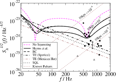
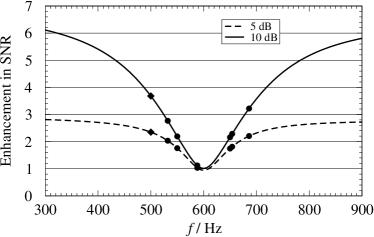
Figure 7: Noise curves of non-squeezed (light dashed curve), Harms et al. (dark continuous curves) and BC (dark dashed curves) configurations optimized for narrowband sources, for 5 dB and 10 dB squeezing. We apply only one filter, that is the one with resonant frequency near the free optical resonant frequency of the SR interferometer, or filter I (see Table V.1). The interferometer noise curves contain only quantum noise but include filter losses. The thermoelastic noise of spherical and MH mirrors, and the SQL are plotted for comparison. We also show the frequencies and characteristic strengths (20-day coherent integration, $1\%$ false alarm BCCS ; BC ) of possible GWs from LMXBs B98 [using the baseline assumption (a1), namely $f_{s}=f_{d}$ and mass-quadrupole emission]: Z sources in solid circles (Sco X-1 in diamond), Type-I X-ray bursters in solid squares and accreting millisecond pulsars in open triangles. For the accreting millisecond pulsar SAX J1808.4–3658, for which the orbital parameters and GW phase evolutions are known SAX , we show in another open triangle (linked to the 20-day one with a vertical segment of solid line) the characteristic strength assuming a 4-month integration.

Figure 8: Relative increase in SNR for LMXB sources around 600 Hz, with 5 dB ($e^{-2r}=0.316$, dashed curve) and 10 dB ($e^{-2r}=0.1$, continuous curve) squeezing. Since the Harms et al. and BC schemes are extremely close to each other only one curve is shown for each squeeze factor. The various detectable LMXBs [under the baseline assumption] listed in Table V.1 are also shown (Sco X$-$1 in solid diamond, the rest in solid circles) .

Moreover, two plausible physical mechanisms for GW emission from accreting NS’s have been proposed: (1) mass quadrupole radiation from deformed NS crusts ($f_{\rm GW}=2f_{s}$) old ; B98 ; and (2) current quadrupole radiation from unstable (with respect to gravitational radiation) pulsation modes (r-modes) in NS cores ($f_{\rm GW}=4f_{s}/3$) rmode ; OLCSVA ; AKS . Suppose one of the two emission mechanisms to dominate, then along with uncertainties in spin frequencies, we have four possibilities for Z sources, (a1), (a2), (b1) and (b2); [and two possibilities for accreting millisecond pulsars and Type-I bursters, (1) and (2)]. In the following, we consider (a1) for Z sources and (1) for accreting millisecond pulsars and Type-I bursters our baseline assumption, as done in Refs. B98 ; UBC ; LB02 ; CT , and comment on what happens if the other options turn out to be true.

In the second column of Table V.1, we list GW frequencies obtained from the baseline assumption; GW frequencies based on other assumptions can be obtained from the (a1) or (1) value by using Table 6. The characteristic GW amplitude $h_{c}$ from LMXBs has been estimated UCB ; OLCSVA by assuming a balance between GW angular momentum loss and accretion torque, with the latter estimated from X-ray flux, and by subsequent averaging over the (unknown) spin orientation [see Appendix B.1 for a detailed explanation on the averaging process and the associated uncertainties]. However, the value of $h_{c}$ can also be different due to the various assumptions on spin frequency and GW emission mechanism we can make. Values listed in the third column of Table V.1 has been obtained in Refs. B98 ; UBC ; LB02 using the baseline assumption; conversions from (a1) or (1) to the other assumptions can be made easily using Eq. (8) of Ref. UCB and Eqs. (4.4)–(4.6) of Ref. OLCSVA , and are given in Table 6. By assuming $1\%$ false-alarm probability and 20-day coherent integration time [due to unknown orbital motion and frequency drifts caused by fluctuations in the mass accretion rate] $S_{h_{c}}$ can be obtained from $h_{c}$ (listed on the fourth column of Table V.1, see App. B.2 for details), note that for the different assumptions $\sqrt{S_{h_{c}}}$ changes by the same factor as $h_{c}$. For the accreting millisecond pulsar SAX J1808.4–3658, for which the orbital motion is known CM98 , assuming that GW frequency evolution can be obtained, we also show (in parenthesis) the characteristic strength obtained with a 4-month integration.

It is important to realize that there are still uncertainties as to whether a particular source will be detectable, even if the noise curve is below $S_{h_{c}}$ — as explained in Appendix B. However, the main aim of this paper is to discuss interferometer configurations, rather than the data analysis of narrowband sources, so we shall use $S_{h_{c}}$, as done by Cutler and Thorne CT despite the subtleties, as a playground to compare sensitivities of different interferometer/filter configurations. Conclusions drawn in our discussions on whether these sources will be detectable should definitely be refined by more rigorous investigations.

In Fig. 8 we plot the noise curves obtained for a non-squeezed SR interferometer and for squeezed SR interferometers with the Harms et al. and BC schemes by optimizing their sensitivities in a narrow band around 600 Hz. Peak sensitivities and bandwidths are adjusted to incorporate the signal strengths of a group of 7 Z sources (including Sco X-1). The baseline assumption is used in obtaining $f_{\rm GW}$ and $S_{h_{c}}$ for these sources.

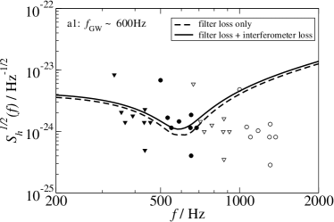
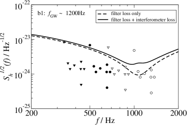
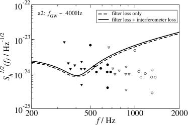
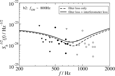
Figure 9: Consequences of spin-frequency and emission-mechanism uncertainties on the detection of LMXBs (Z sources) using narrowband configurations. We plot the GW frequency and characteristic GW strength (for 20-day coherent integration), under approximations (a1) (solid circles with center frequency around 600 Hz), (b1) (open circles, with center frequency around 1200 Hz), (a2) (solid triangles, with center frequency around 400 Hz) and (b2) (open triangles, with center frequency around 800 Hz), along with Harms et al. (equivalent to BC) noise curves (with 10 dB squeezing) tuned to those frequencies, with (solid curves) and without (dashed curves) internal losses of the interferometer. We assume an ITM power transmissivity of $0.033$, SR-cavity round-trip loss of $1\%$ and photodetection loss of $2\%$; $I_{c}=840$ kW and $m=40$ kg. The rest of the parameters are listed in Table 8.

assumption	$\displaystyle\frac{f_{\rm central}}{\rm Hz}$	$\displaystyle\frac{\epsilon}{2\pi{\rm Hz}}$	$\displaystyle\frac{\lambda}{2\pi{\rm Hz}}$	$\zeta$
(a1)	600	30	600.4	$-0.756$
(b1)	1200	90	1057.3	$-0.065$
(a2)	400	25	412.6	$-0.749$
(b2)	800	90	769.0	$-0.306$

Table 8: Parameters of narrowband configurations tuned to LMXB sources when different assumptions on spin frequency and GW emission mechanism are adopted. Noise curves of these configurations, with and without interferometer losses included, are shown in Fig. 9, and compared to the corresponding GW characteristic strengths.

For the non-squeezed interferometer, we obtain a noise curve similar to the “narrowband” curve in Fig. 1 of Cutler and Thorne CT , provided originally by Ken Strain. For squeezed interferometers, we have considered both 5 dB ($e^{-2r}=0.316$) and 10 dB ($e^{-2r}=0.1$) squeezing. Since in narrowband configurations, the seismic and thermal noises do not affect significantly the choice of the SR parameters, the noise curves in Fig. 8 have been optimized using only the quantum-optical noise (but we include filter optical losses). [For comparison we plot in Fig. 8 the thermoelastic noises.] We obtain the parameters $\epsilon$, $\lambda$ and $\zeta$ for the squeezed configurations following a heuristic procedure. Since the filters are very lossy, it is desirable to increase $\epsilon$ from the non-squeezed value, $2\pi\times 25\,$Hz, so that the noise due to filter losses decreases and although the ideal minimum of $S_{h}^{\rm lossless}$ increases, it is still buried by the noise due to filter losses. As we increase $\epsilon$ from $2\pi\times 25\,$Hz, we search for the $\lambda$ and $\zeta$ that minimize $S_{h}$ at 600 Hz; we find that the sensitivity at 600 Hz remains roughly the same, while the bandwidth increases. Trying to include as many sources as possible, we set $\epsilon=2\pi\times 100\,$Hz for 5 dB squeezing and $2\pi\times 60\,$Hz for 10 dB squeezing. The interferometer and filter parameters used in these configurations are listed in Table. 7.

As we see from Fig. 8, the Harms et al. [two dark continuous lines, one for 5 dB squeezing the other for 10 dB squeezing] and the BC [two dark dashed lines] schemes are extremely close to each other. The peak sensitivities in the 5 dB and 10 dB cases are chosen to be comparable to each other, while 10 dB squeezing gives a broader band. Although the FD techniques cannot increase the peak sensitivity much due to filter losses, they do increase the bandwidth of observation. This will allow the observation of multiple possible sources with a fixed configuration. For example, with the frequency and GW strengths estimates we used in Fig. 8, with 10 dB squeezing, we can detect simultaneously 7 sources near 600 Hz (including Sco X-1), while with 5 dB squeezing we can detect 6 of them simultaneously (including Sco X-1). In Fig. 8, we plot the increase in SNR by the squeezed schemes, as compared to the non-squeezed schemes, for LMXBs around the resonant frequency; both 5 dB and 10 dB squeezing are shown. In Table V.1, columns 5–9 we list the sensitivies of these configurations.

As in the case of NS binary inspirals, SR interferometers with frequency-independent squeezing and readout phase can also be optimized for the detection of LMXBs. However, squeezing combined with frequency-independent input-output optics cannot easily improve peak sensitivity and bandwidth at the same time for narrowband configurations. As a consequence, as we optimize the frequency-independent scheme with 5 dB squeezing, we obtain narrowband configurations that can detect at most 4 sources out of the group of 7 (including Sco X-1). [With 10 dB squeezing, when a similar optimization is done for frequency-independent schemes, one finds that a wideband interferometer with frequency-independent scheme can detect all 7 sources — no narrowbanding is necessary, as we shall see in the next section.]

Now we look at the interferometer performances if assumptions other than (a1) turn out to be true. In Fig. 9, we show the predicted GW strengths from the Z sources under the four assumptions (obtained using Tables V.1 and  6): (a1) (solid circles, with center frequency around 600 Hz), (b1) (open circles, with center frequency around 1200 Hz), (a2) (solid triangles, with center frequency around 400 Hz) and (b2) (open triangles, with center frequency around 800 Hz). Given these hypothetical groups of sources, we tune squeezed-input SR interferometers (with Harms et al. or BC schemes, which are equivalent at high frequencies) to each of them: around 600 Hz, 1200 Hz, 400 Hz, and 800 Hz, with interferometer parameters listed in Table 8 and noise curves shown in Fig. 9. We remark that assumptions that yield lower $f_{\rm GW}$’s tend to make the sources more detectable. In this study, we have also taken into account interferometer losses, which has been neglected up till now. We assume the ITM power transmissivity to be $T=0.033$, SR-cavity round-trip loss to be $1\%$ (denoted by $\lambda_{\rm SR}$ in Ref. BC2 ) and photodetection loss to be $2\%$ (denoted by $\lambda_{\rm PD}$ in Ref. BC2 ). These numbers are crude estimates; given the effects of interferometer losses suggested by Fig. 9, especially in higher frequencies [i.e., if assumptions (b1) or (b2) turns out to be true], more refined understanding of realistic interferometer losses, as well as a more systematic study of interferometer parameters will be crucial in fully understanding whether and how Advanced LIGO can detect these narrowband sources.

Interferometer Configuration Filter I Filter II Performance 10 dB [5 dB] Scheme $\displaystyle\frac{\epsilon}{2\pi\,{\rm Hz}}$ $\displaystyle\frac{\lambda}{2\pi\,{\rm Hz}}$ $\alpha$ $\zeta$ $\displaystyle\frac{\Omega_{\rm res}^{\rm I}}{2\pi\,{\rm Hz}}$ $T_{i}^{\rm I}$ (ppm) $\displaystyle\frac{\Omega_{\rm res}^{\rm II}}{2\pi\,{\rm Hz}}$ $T_{i}^{\rm II}$ (ppm) $\sqrt{S_{h}}/(10^{-24}/\sqrt{{\rm Hz}})$ at 600 Hz NS-NS at 300 Mpc Spherical/MH No Filters $600$ $0$ $\pi/2$ $0$ $0.99$ [$1.77$] 6.47/8.70 [5.69/7.60] Harms et al. $600$ $0$ FD $0$ $2.8-600.0\,i$ 1508 $-41.3-41.0\,i$ 103 $1.12$ [$1.82$] 7.00/10.65 [6.01/8.76] BC $600$ $0$ $\pi/2$ FD $2.8-600.0\,i$ 1508 $-41.3-41.0\,i$ 103 $1.13$ [$1.85$] 6.68/9.68 [5.79/8.09]

Table 9: Parameters of wideband configurations, including: squeezing with frequency independent input-output optics, the Harms et al. scheme and the BC scheme. Since there is no detuning in these SR interferometers, they are equivalent to conventional interferometers, which KLMTV studied. We also give the noise spectral densities at 600 Hz, and the SNR for NS-NS binaries at 300 Mpc distance. Both 5 dB and 10 dB squeezing are considered, with 5 dB numbers quoted in parentheses, “[…]”. In cases with 10 dB squeezing, the sensitivties at 600 Hz is only slightly worse than the narrowband configurations (see Table 7).

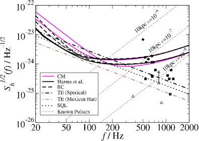
Figure 10: Noise spectral densities of wideband configurations, with $\epsilon=2\pi\times 600\,$Hz and $\lambda=0$, frequency-independent squeezing ($\alpha=\pi/2$, $\zeta=0$, light continuous curve), the Harms et al. scheme ($\zeta=0$, dark continuous curve) and the BC scheme ($\alpha=\pi/2$, dark dashed curve) are used. Only the quantum-optical noise (taking filter losses into account) is included. Thermoelastic noises of spherical and MH mirrors are also shown, in dark and light dash-dot lines, respectively. The SQL is shown in dashed line. Possible GW signals from LMXBs [under the baseline assumption] and known radio pulsars are also shown.

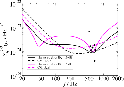
Figure 11: Comparison of sensitivities to LMXB sources. We plot the noise curves of Harms et al. (or equivalently BC) scheme (continuous curves) and with frequency independent squeezing and readout scheme (the CM configuration, dashed curves), with 5 dB (light curves) and 10 dB (dark curves) squeezing. We also plot the estimated frequencies and characteristic GW strengths of Sco X-1 and several other Z sources [under the baseline assumption (a1)].

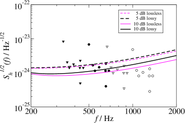
Figure 12: Consequences of spin-frequency and emission-mechanism uncertainties on the detection of LMXBs (Z sources) using the wideband configuration. We plot the GW frequency and characteristic GW strength (for 20-day coherent integration), under approximations (a1) (solid circles), (b1) (open circles), (a2) (solid triangles) and (b2) (open triangles), along with CM noise curves with 5 dB (dashed curves) and 10 dB (continuous curves) squeezing, with (dark curves) and without (light curves) interferometer losses.

V.3 Wideband configuration

The so-called wideband configuration of SR interferometers can be obtained setting $\lambda$ small and $\epsilon$ rather high. These configurations can be used to detect a broad range of generic sources, including: coalescence of NS-NS binary, tidal disruption of NS by the BH companion, accreting NS’s and radio pulsars. There are no specific criteria for the noise spectrum of the wideband configuration. For simplicity we set $\epsilon=2\pi\times 600\,$Hz and $\lambda=0$ (since this configuration is similar to the one by Corbitt and Mavalvala CM , we denote it by CM). The various parameters used are summarized in Table 9, along with SNR achievable for NS binaries at 300 Mpc and sensitivities at 600 Hz. Both 5 dB and 10 dB squeezing are considered, with 5 dB numbers quoted in parentheses, “[…]”. We plot the corresponding noise curves in Fig. 10.

For frequencies higher than 200 Hz, the CM noise curves are always better than those with FD techniques. This is because, as observed by Corbitt and Mavalvala, at high frequencies, the optimal squeeze angle and detection phase depend very mildly on the frequency. Therefore, the FD schemes, having additional filter losses, give worse performances. At high frequencies, the wideband schemes give a sensitivity of $3.2$ (10 dB squeezing) or $1.8$ (5 dB squeezing) times better (in amplitude) than the wideband configuration without squeezing. With 10 dB squeezing, the wideband configurations can detect known pulsars at 10 kpc with $\epsilon\stackrel{{\scriptstyle>}}{{{}_{\sim}}}10^{-7}$ if $f_{\rm GW}\stackrel{{\scriptstyle>}}{{{}_{\sim}}}420\,$Hz, with $\epsilon\stackrel{{\scriptstyle>}}{{{}_{\sim}}}3\times 10^{-8}$ if $f_{\rm GW}\stackrel{{\scriptstyle>}}{{{}_{\sim}}}1\,$kHz. [With 5 dB squeezing, the minimum detectable $\epsilon$ will be 1.8 times larger than the 10 dB value.] However, if we also require good sensitivities below 200 Hz, then the FD wideband schemes are preferable to the CM configuration .

In addition, in the 10 dB squeezing case, when spherical mirrors are used, the SNR for binaries are all above $96\%$ the optimal values obtained in the broadband case (see Table 4). However, for Mexican-Hat mirrors, the SNR is less optimal, equal to $83\%$ (no filters), $91\%$ (Harms et al.) and $93\%$ (BC) the optimal values (of the same scheme). [See Table 4.] These can be understood by going back to Sec. V.2 and observing in (the left panel of) Fig. 6 that for spherical mirrors, the optimal noise curves are very wideband.

It is also interesting to note that, with 10 dB squeezing, the sensitivities of wideband configurations around 600 Hz, are only slightly worse, $\sim 10\%$ in amplitude, than the narrowband configurations. As a consequence, with 10 dB squeezing, the wideband configurations, even without FD techniques, can detect the same groups of LMXBs discussed in the last section (see Fig. 10). However, it should be noted that, if 10 dB squeezing is not achievable, then one cannot detect these sources with the wideband configuration. For example, 5 dB squeezing will barely allow one or two more LMXBs than Sco X-1 to be detected. The narrowband configuration (with FD input-output schemes), by contrast, will only miss one source in the group of 7. In Fig. 11, we compare the sensitivities of narrowband FD schemes and wideband frequency independent schemes to LMXB sources, with 5 dB and 10 dB squeezings.

Finally, by taking into account all other assumptions on spin frequency and GW emission mechanism, we plot in Fig. 12, the predictions of (a1), (b1), (a2) and (b2), along with CM noise curves with 5 dB (dashed curve) and 10 dB squeezing (continuous curve), with (dark curves) and without (light curves) interferometer losses included.

VI Third-generation interferometers

We now assume that on time scales of third-generation GW interferometers (around 2012), thermal noise of mirrors will be reduced by a large factor, for example by using cryogenic techniques, and we can take full advantage of the improvements in quantum noise obtained by FD input-output techniques. In addition, we assume that long filters can be fit into the existing vacuum tubes (which house the arm cavities) of the LIGO facility and made 4 km long, so that optical losses will be significantly lowered (see Table 3). As discussed in Sec. IV.4, the BC scheme is nearly optimal for frequencies lower than the optical resonance [see Fig. 5 and Eq. (102)], thus in the following we shall restrict our analysis to the BC scheme. However, before showing the performances, we want to discuss the limitations of the so-called short-cavity approximation, so far used in the literature to describe kilometer-scale filter cavities  KLMTV00 ; ligoIII:sm .

VI.1 Breakdown of short-cavity approximation

Up till now in this paper, we have been using the short-cavity approximation, which imposes that $\Omega L/c\ll 1$. [Note that when refered to the interferometer, $L$ is the arm length, $\Omega$ is the GW sideband frequency or the optical resonant frequency $-\lambda-i\epsilon$; when refered to filter cavities, $L$ is the filter length, $\Omega$ is the GW sideband frequency or the filter resonant frequency $\Omega_{\rm res}$.] As we saw in Secs. II and III, the short-cavity approximations, applied to SR interferometers and KLMTV filters, simplify significantly their input-output relations [see Eqs. (3)–(5), (43) and (47)], allowing a straightforward determination of filter parameters in the Harms et al. and BC schemes via characteristic equations [Eqs. (80) and (83)].

On the contrary, without this approximation (i.e., when cavity lengths are too long for this approximation to work), the filter parameters cannot be determined easily — it is not even clear whether the optimal/suboptimal frequency dependence required by (the exact input-output relation of) SR interferometers can at all be realized by (those of) KLMTV filters.

Since we have derived the exact input-output relation of the filters [Eqs. (57)–(59)], as well as (partially) that of the interferometer [Eqs. (99)–(104) of Ref. BC5 ], we can investigate the range of validity of the short-cavity approximations.

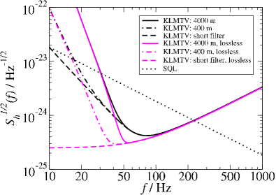
Figure 13: To show the break-down of the short-cavity approximation we plot several noise curves for the KLMTV (conventional) squeezed-variational interferometer KLMTV00 with $I_{c}=840$ kW, $m=40\,$kg and $e^{-2r}=0.1$, fixing a bandwidth of $\epsilon=2\pi\times 75$ Hz. The dark continuous curve refers to the nominal filter-cavity length $L_{f}=4$ km, and the round-trip filter loss $T_{e}=20\,$ppm; while the short-filter approximation ($L_{f}=0.1\,{\rm m}$) predicts the dark dashed curve. For comparison, we also plot noise curves of configuration with $L_{f}=400\,$m, $T_{e}=2\,$ppm (dark dash-dot curve), along with those of the lossless optical configurations with $L_{f}=4\,$km (light continuous curve), $L_{f}=400\,$m (light dash-dot curve) and with short-filter approximation ($L_{f}=0.1\,{\rm m}$) (light dashed curve).

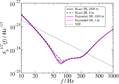
Figure 14: To investigate the short-filter and short-arm approximation in SR squeezed-variational interferometers we plot several noise curves fixing $I_{c}=840$ kW, $m=40\,$kg, $e^{-2r}=0.1$, $\epsilon=2\pi\times 80\,$Hz and $\lambda=2\pi\times 200\,$Hz. In particular we show the noise curve obtained with exact input-output relation and 4 km filter cavities (dark continuous curve), and 4 m filter (dark dashed curve); the noise curves obtained with first-order expanded input-output relation and 4 km filter (light continuous curve) and 4 m filter (light dashed curve). We use $T_{e}=20$ ppm for the 4 km configurations, and $T_{e}=0.02$ ppm for 4 m configurations, such that the overall loss factor remains the same. The disagreements between curves with the same pattern (continuous or dashed) but different color (dark or light) is due to the inaccuracy of short-filter approximation; while the disagreements between curves with the same color but different pattern is due to the inaccuracy of short-arm approximation.

Let us start with conventional interferometers. As we have checked in this case, the short-arm approximation is still quite accurate, in the sense that, for a given readout scheme (i.e., a given set of input or output filters), using exact and short-arm–approximated input-output relation do not give very different results. Yet, the short-filter approximation seems to lose accuracy at low frequencies. We study this effect in Fig. 13, by plotting several noise curves for squeezed-variational conventional interferometers KLMTV00 with $I_{c}=840\,$kW, $m=40\,$kg, $e^{-2r}=0.1$, and $\epsilon=2\pi\times 75\,$Hz, using the exact interferometer input-output relation. In doing so, we use filters with bandwidths and resonant frequencies obtained from the short-filter approximation, but with different actual lengths and losses. In the figure, we show the noise curve for filters with $L_{f}=4\,$km and $T_{e}=20\,$ppm in dark continuous curve, and also lossy filters with decreasing length but the same $T_{e}/L_{f}$ ratio: $L_{f}=400\,$m in dark dotted curve and $L_{f}=0.1\,$m (to simulate short-filter limit) in dark dashed curve. The noise spectrum improves as the filter length decreases. [In fact, since in this case the short-arm approximation is accurate, short filters must give the optimal performance.] In Fig. 13, we also show noise curves for lossless configurations with $L_{f}=4\,$km in light continuous curve, $L_{f}=400\,$m in light dotted curve and $L_{f}=0.1\,$m (to simulate short-filter limit) in light dashed curve. The reason for such dramatic noise increase at low frequencies can be attributed to the strong ponderomotive squeezing generated by conventional interferometers at these frequencies (note that $q\rightarrow+\infty$ as $\Omega\rightarrow 0$, see left panel of Fig. 1). The stronger the squeezing, the higher the accuracy requirement on the FD readout phase; yet the accuracy of short-filter approximation does not increase indefinitely when $\Omega\rightarrow 0$.

By contrast, as we have checked, the short-cavity approximations still apply very well to squeezed-input conventional interferometer which at low frequencies does not have as good an ideal sensitivity as the squeezed-variational conventional interferometer.

In Fig. 14 we investigate the short-arm and short-filter approximations for SR squeezed-variational interferometers (the BC scheme) with $I_{c}=840\,$kW, $m=40\,$kg, $e^{-2r}=0.1$, $\epsilon=2\pi\times 80$ Hz and $\lambda=2\pi\times 200\,$Hz. In this case, both the short-filter and short-arm approximations introduce some inaccuracies, but they are by far not as significant as in the squeezed-variational conventional interferometers. In particular, in Fig. 14, we plot noise curves obtained using exact interferometer input-output relation, with 4 km (dark continuous curve) and 4 m filters (dark dashed curve), and noise curves obtained using short-arm–approximated interferometer input-output relation, with 4 km (light continuous curve) and 4 m (light dashed curve) filters. We fix $T_{e}=20\,$ppm for 4 km configurations, and $0.02\,$ppm for 4 m configurations, keeping the same overall loss factor. [Filter resonant frequencies and bandwidths are still obtained from the characteristic equation (83), which in turn has been derived based on both short-arm and short-filter approximations]. Noise curves with the same color (light or dark) use the same interferometer input-output relation, so the difference between them reflects the inaccuracy of the short-filter approximation; those with the same pattern (continuous or dash) share the same filter input-output relation, so their difference reflects the inaccuracy of the short-arm approximation. We conclude that the errors arising from the short-arm and short-filter approximations somewhat cancel each other, making the exact noise curve differ only slighly from the curve with both short-arm and short-filter approximations applied. The mild noise increase around the optical-spring resonance in this case can also be understood from the ponderomotive squeezing factor. As we see from the left panel of Fig. 1 (the dashed curve represents a similar configuration), ponderomotive squeezing is the strongest near this resonance, yet even here the squeeze factor is still small compared to that of the conventional interferometer at lower frequencies.

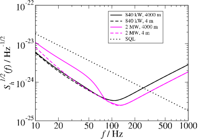
Figure 15: We plot the noise curves of squeezed-variational speed meters with $\Omega_{\rm s}=2\pi\times 95.3\,$Hz, $\delta=2\pi\times 100\,$Hz, and $e^{-2r}=0.1$, assuming $I_{c}=840\,$kW (dark curves) and $I_{c}=2\,$MW (light curves), and $L_{f}=4000\,$m (continuous curves) and $L_{f}=4\,$m (dashed curves). The round-trip losses are $T_{e}=20$ ppm for 4000 m filters and $T_{e}=0.02\,$ppm for 4 m filters. The optical losses are included following Ref. PC02 .

We now discuss the short-cavity approximation in squeezed-variational speed meters ligoIII:sm ; ligoIII:sag . We consider the configuration with $\Omega_{\rm s}=2\pi\times 95.3\,$Hz (the “sloshing frequency”, as denoted by $\Omega$ in Ref. PC02 ) and $\delta=2\pi\times 100\,$Hz (bandwidth), assuming $e^{-2r}=0.1$. We include optical losses as done in Ref. PC02 . As for conventional squeezed-variational interferometers, the short-arm approximation is rather accurate here. [This is true if the enhanced formula (i.e., expanded to next-to-leading order in $\Omega L/c$) for the quantity $\kappa$ is used, see footnote 5 of Ref. PC02 .] However, the short-filter approximation is not accurate enough, if we increase the optical power further from Advanced LIGO value. In Fig. 15, we plot four noise curves with $I_{c}=840\,$kW (dark curves) and $2\,$MW (light curves), and filter lengths 4000 m (and $T_{e}=20\,$ppm, continuous curves) and 4 m (and $T_{e}=0.02\,$ppm, dashed curves). [Again, resonant frequencies and bandwidths of the filters are obtained in the same way as in Ref. PC02 , based on short-arm and short-filter approximations.] As we see, a filter length of 4000 m increases the noise significantly as $I_{c}$ becomes on the order of 2 MW. The increase is rather constant (and now as dramatic as in KLMTV squeezed-variational conventional interferometers) at low frequencies, because speed meters have a constant ponderomotive squeezing factor at low frequencies PC02 .

We notice that in all the above cases where the short-cavity approximations break down, using filter parameters obtained from the characteristic equations (as we have done above), which are derived assuming those approximations, can no longer be optimal. Instead, one must optimize filter parameters numerically using exact filter and interferometer input-output relations. We do not have quantitative results yet on how much sensitivity can be gained by this re-optimization, but it does not seem likely that the sensitivity can reach the optimal level (i.e., having the FD rotation from the filters matching exactly the interferometer’s requirement).

VI.2 Performances of SR squeezed-variational interferometers

Using exact filter and interferometer input-output relations (i.e., without applying short-cavity approximations), and assuming that 4 km filters will be used in third-generation interferometers, we compare in Fig. 16 the noise spectral densities of conventional squeezed-variational interferometers, SR squeezed-variational interferometers (BC scheme), and the squeezed-variational and -input speed meters. The BC scheme (which requires two additional km-scale cavities) has better sensitivity than the conventional squeezed-variational scheme (which also requires two additional km-scale cavities) for all frequencies below $\sim$350 Hz. It has also better performances than the squeezed-input speed meter (which requires one additional km-scale cavity) for all frequencies above $\sim$40 Hz. The BC scheme has comparable (or slightly better) sensitivities with respect to the squeezed-variational speed meter (which requires three additional km-scale cavities) for frequencies between $\sim 50$ Hz and $\sim 300\,$Hz.

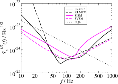
Figure 16: Noise spectral densities of SR interferometers with BC scheme (SR+BC, dark continuous line), conventional squeezed-variational interferometer (KLMTV, dark dashed line), the Purdue-Chen speed-meter interferometer with ordinary homodyne detection (light continuous line) and FD homodyne detection (light dashed curve). We assume $I_{c}=840\,$kW, $m=40\,$kg and $e^{-2r}=0.1$; the SR interferometer with BC scheme has $\lambda=2\pi\times 200\,$Hz, $\epsilon=2\pi\times 80\,$Hz and $\alpha=\arctan(\epsilon/\lambda)$; the speed meter with ordinary homodyne detection has $\Omega_{s}=173.2\,$Hz and $\delta=2\pi\times 200$ Hz, while the speed meter with FD homodyne detection has $\Omega_{s}=2\pi\times 95.3\,$Hz and $\delta=2\pi\times 100\,$Hz. Optical filters are assumed to be 4 km long, with 20 ppm round-trip loss.

VII Conclusions

In this paper, we generalized the study of KLMTV KLMTV00 on FD input-output optics to SR interferometers, and discussed possible applications to second- and third-generation GW interferometers.

In the first part of the paper (Secs. II – IV), we studied the quantum optical properties of SR interferometers and FD input-output schemes. We wrote the input-output relations of SR interferometers as a product of ponderomotive squeezing and quadrature rotations, deriving explicit formulas for the intrinsic rotation angle and squeeze factor [see Eqs. (25) and (26)], and investigating their features for several optical configurations. We found that ponderomotive squeezing becomes very weak in SR interferometers for frequencies higher than $\sim 300\,$Hz, regardless of the optical configuration [see Eq. (30)]. Then, we built and analyzed the performances of the input-output scheme which combine FD homodyne detection (via KLMTV filters) with ordinary input squeezed vacuum (BC scheme), and compared it to the recent FD scheme proposed by Harms et al. Harms03 . In the low-power limit (which also describes the high-frequency band of Advanced LIGO) we worked out the fully optimal input-output scheme [see Eq. (92)]. In the general case, we derived simple analytical formulas for the fully optimal noise spectrum [Eq. (99)] and the optimal input squeeze angle [Eq. (98)], and found that at low frequencies, the BC scheme can approximate the fully optimal noise curve very well [see Eq. (102)], providing better perfomances than the Harms et al. scheme. These results for SR interferometers are quite similar to the conventional interferometer case, in which as shown by KLMTV, a frequency independent squeezed vacuum is already fully optimal (with FD readout), yet a frequency independent readout cannot give as good a sensitivity (even with FD squeezing). [The BC and Harms et al. schemes generalize to SR interferometers the squeezed-variational and squeezed-input schemes introduced by KLMTV for conventional interferometers.]

In the second part of the paper (Sec. V), assuming that squeezed vacuum in the GW band would become available during the operation of Advanced LIGO, we evaluated the improvement in astrophysical sensitivity to specific sources achievable by these FD schemes, under the facility limitation that the filters cannot be longer than $30\,$meters. It is important to note that, as has been realized by Corbitt and Mavalvala CM , for nearly tuned SR interferometers with a large bandwidth (wideband configuration), the optimal input-output scheme is nearly frequency independent at high frequencies. So, in this case it is possible to use squeezing optimally without introducing FD techniques. The Corbitt-Mavalvala (CM) wideband configuration can be used to detect simultaneously various types of sources in the high-frequency band, e.g., NS-NS merger, tidal disruption in NS-BH systems, or GWs from known radio pulsars. In addition, if 10 dB squeezing can be realized, this wideband configuration can already detect a group of 7 LMXBs (including Sco X-1) around 600 Hz.

However, for specific sources with known spectral features, it is more convenient to use optical configurations which are not wideband. In this case, the FD techniques can provide more flexibility and somewhat better sensitivity, despite significant optical losses due to short filters. The Harms et al. scheme is shown to provide a better sensitivity than the BC scheme in general in the Advanced LIGO era, due to the BC scheme’s higher susceptibility to losses at low frequencies and the filter-length limitation to 30 meters. For NS-NS inspirals, assuming 10 dB squeezing, without using FD filters, one can improve the event rate by $89\%$ (spherical mirror) or $42\%$ (MH mirror) with respect to the non-squeezed case; further improvements of $20\%$ (spherical mirror) and $42\%$ (MH mirror) can be obtained by the Harms et al. scheme. For LMXBs, using 5 dB squeezing, without using FD techniques, the broadband configuration can only detect 3 sources simultaneously. By adjusting the SR parameters, we find that a frequency independent input-output scheme cannot detect more than 4 sources, since in this case we cannot gain sensitivity and bandwidth at the same time. The Harms et al. and BC schemes, instead can allow the detection of 6 sources simultaneously, by opening up the bandwidth with FD filters (although the peak sensitivity cannot be improved much due to significant filter losses). With 10 dB squeezing, the Harms et al. and BC schemes can open up the bandwidth further, including a group of 7 sources near 600 Hz. [However, with this level of squeezing, the broadband configuration can also detect the same sources, though with slightly less sensitivity.] It is important to mention that, the above detailed results about LMXBs are obtained by assuming (baseline assumption) that the Z sources, which are the most promising GW sources among all the LMXBs, are spinning at the QPO difference frequency ($f_{s}=f_{d}\approx 300\,$Hz) and that the GW is dominantly mass-quadrupole emission ($f_{\rm GW}=2f_{s}\approx 600\,$Hz). Recent results SAX , however, may suggest that the spin frequencies could be twice the QPO difference frequency and therefore lie around $600\,$Hz instead. In addition, it is not clear yet whether the dominant GW emission is mass quadrupole (e.g., due to deformation in the crust) or current quadrupole (e.g., due to r-mode). In Figs. 9 and 12, we have briefly explored the sensitivities of narrowband and wideband configurations to these alternative scenarios. Moreover, we also realized that optical losses inside the SR interferometer become rather crucial in deciding whether these sources will be detectable, especially if the predicted waves are at higher frequencies. A more careful study of optical losses will be reported in a forthcoming paper BC7 . It should also be remembered that we have been relying on the characteristic GW strength CT of LMXBs to provide a very rough criterion of detectability — in order to make a straightforward yet specific comparison between different noise curves. As a consequence, the true detectability of these sources by configurations studied in this paper should be refined by a more rigorous study.

In the third part of the paper (Sec. VI), we investigated the performances of squeezed SR interferometer with FD output using two 4-km KLMTV filter cavities. We found [see Fig. 16] that SR interferometers with input squeezing and sub-optimal FD readout scheme (the BC scheme) can have competing sensitivities to existing proposals for third-generation interferometers ligoIII:sm ; ligoIII:sag , especially in the middle frequency band of $50$ – $350\,$Hz (see Fig. 16) . We also discuss the limitation of the short-arm and short-filter approximations adopted by most of the past works KLMTV00 ; ligoIII:sm . Should at least one of these approximations break down, the optimal (or suboptimal) filter parameters provided by the characteristic equation (44) would not give the required FD rotation — which, in fact, may not even be realizable by any sequence of detuned FP cavities. Indeed, we found that for squeezed-variational conventional interferometers and speed meters (with high power), the approximation breaks down at low frequencies if applied to km-scale filters (see Fig. 13 and Fig. 15), which we attribute to the high level of ponderomotive squeezing and therefore more stringent requirement rotation accuracy in these configurations; while for SR squeezed-variational interferometers (BC scheme), the error introduced by the approximations is rather mild (see Fig. 14).

Appendix A Proof that the fully optimal scheme satisfies the sub-optimal condition

Suppose $\zeta$ is the readout phase. As seen in Sec. IV, with the sub-optimal $\alpha$ given by Eq. (76), only the squeezed quadrature enters the detected quadrature. We now show that given $\zeta$, this $\alpha$ is also the optimal squeeze quadrature in the sense that it minimizes the output noise. Since when we vary $\alpha$ alone, the signal strength in the output quadrature $b_{\zeta}$ remains constant, we only need to minimize the noise in $b_{\zeta}$. We write Eq. (86) schematically as

$$\Delta b_{\zeta}=\left(\begin{array}[]{cc}A_{1}&A_{2}\end{array}\right)\mathbf{R}(\alpha)\left(\begin{array}[]{r}e^{-r}\tilde{a}_{1}\\ e^{r}\tilde{a}_{2}\end{array}\right)\,,$$ (109)

with $(A_{1}\,\,A_{2})$ the product of the readout and the interferometer parts, $A_{1,2}\in\Re$. The noise spectrum depends on $\alpha$ as

$$S_{h}\propto\left(\begin{array}[]{cc}A_{1}&A_{2}\end{array}\right)\mathbf{R}(\alpha)\left(\begin{array}[]{cc}e^{-2r}&\\ &e^{2r}\end{array}\right)\mathbf{R}(-\alpha)\left(\begin{array}[]{c}A_{1}\\ A_{2}\end{array}\right)\,.$$ (110)

Minimizing $S_{h}$ then requires

$$\left(\begin{array}[]{cc}A_{1}&A_{2}\end{array}\right)\mathbf{R}(\alpha)\left(\begin{array}[]{c}0\\ 1\end{array}\right)=0\,,$$ (111)

which is equivalent to Eq. (87) and hence to Eq. (76).

Appendix B On the detectability of narrowband sources

In this appendix, we briefly review some subtleties that are not taken into account in our discussion of narrowband sources. We restrict the analysis to the mass-quadrupole radiation mechanism.

B.1 Characteristic amplitude of monochromatic gravitational waves: $h_{c}$

Let us consider a monochromatic source emitting GWs at (angular) frequency $\Omega_{0}\neq 0$:

$$h(t) = F_{+}\,h_{+}\,\cos\Omega_{0}t+F_{\times}\,h_{\times}\,\sin\Omega_{0}t\,,$$ (112)

$$h_{+} = h_{0}\,(1+\cos^{2}i)\,,$$ (113)

$$h_{\times} = 2h_{0}\,\cos i\,,$$ (114)

where we denote with $F_{+},F_{\times}$ the antenna patterns KT and with $i$ the angle that the line-of-sight forms with the spin direction of the neutron star. The quantity $h_{0}$ is an intrinsic GW amplitude depending on the ellipticity of the isolated pulsar, or on the X-ray flux emitted by the LMXB (through the balance between accretion torque and GW radiation-reaction torque), as well as on the distance of the source. Suppose the signal is observed in the time interval $-T_{0}/2<t<T_{0}/2$, then the signal-to-noise ratio (SNR) using optimal matched filtering is:

$${\rm SNR}^{2} = \int_{-\infty}^{+\infty}\frac{d\Omega}{2\pi}\frac{2|\tilde{h}(\Omega)|^{2}}{S_{h}(\Omega)}$$ (115)

$$\simeq \left[\frac{2T_{0}}{S_{h}(\Omega_{0})}\right]\left[\frac{F_{+}^{2}\,h_{+}^{2}+F_{\times}^{2}\,h_{\times}^{2}}{2}\right]\,.$$

Note that Eq. (115) differs from Eq. (29) of Ref. KT — the latter is wrong by a factor of 2 KT_private . As we shall see in the next section, when statistical issues are considered, signals above a certain threshold SNR will be detectable.

In reality $F_{+,\times}$ vary due to earth’s motion, or are unknown for some sources; the inclination angle $i$, although may stay constant, could also be unknown, even for known sources, e.g., LMXBs. As a consequence, with a fixed $h_{0}$, the SNR achievable can be different. If we are interested in expected event rates, we should average the SNR over different source and detector orientations. If we want to understand the detectability of a particular source and extract an upper limit, we should consider unfavorable geometries. In this paper the predictions for LMXBs and isolated pulsars have been obtained averaging the SNR. As said, this is not appropriate for evaluating the detectability of individual sources. In what follows we shall briefly review the average procedure, and comment on what might be done in order to extract upper limits from a specific source.

Let us first consider the variation or uncertainty in $F_{+,\times}$. The most straightforward ansatz for taking this into account is to use the r.m.s. average of SNR over the entire sky — as viewed by the detector. The ansatz gives:

$$\sqrt{\langle{\rm SNR}^{2}\rangle_{\rm det}} = \sqrt{2}\,\langle F_{+}^{2}\rangle^{\frac{1}{2}}\sqrt{\frac{T_{0}}{S_{h}(\Omega_{0})}}\sqrt{\frac{h_{+}^{2}+h_{\times}^{2}}{2}}$$ (116)

$$\equiv\frac{1}{h_{n}(\Omega_{0})}\sqrt{\frac{h_{+}^{2}+h_{\times}^{2}}{2}}\,.$$

To obtain the RHS in the above equation we use $\langle F_{+}^{2}\rangle=\langle F_{\times}^{2}\rangle=1/5$, and define [as done in Eq. (51) of Ref. KT ]:

$$h_{n}(\Omega_{0})\equiv\sqrt{\frac{S_{h}(\Omega_{0})/T_{0}}{2\langle F_{+}^{2}\rangle}}\,.$$ (117)

Now let us consider the dependence of $\sqrt{\langle{\rm SNR}^{2}\rangle_{\rm det}}$ on $i$. There are two plausible averaging prescriptions. The first, which is the easiest, and most appropriate for a known source at a fixed distance, averages ${\rm SNR}^{2}$ uniformly over source angles, as

$$\sqrt{\langle{\rm SNR}^{2}\rangle_{\rm det\,\&\,src}} = \frac{1}{h_{n}}\sqrt{\int\frac{d\Omega_{\rm src}}{4\pi}\left(\frac{h_{+}^{2}+h_{\times}^{2}}{2}\right)}$$ (118)

$$= \frac{1}{h_{n}}\,\left(\sqrt{\frac{8}{5}}\,h_{0}\right)\,.$$

It is then natural to define as characteristic amplitude:

$$h_{a}=\sqrt{\frac{8}{5}}\,h_{0}\approx 1.26\,h_{0}\,.$$ (119)

Another way of averaging was proposed by Thorne in Ref. KT , which has the property that $\mbox{event rate}\propto\langle{\rm SNR}\rangle^{3}$, if we assume uniform distribution of sources in the universe,

$$\langle{\rm SNR}\rangle_{\rm det\,\&\,src} = \left[\int\frac{d\Omega_{\rm src}}{4\pi}\left[\langle{\rm SNR}^{2}\rangle_{\rm det}\right]^{\frac{3}{2}}\right]^{\frac{1}{3}}$$ (120)

$$= \frac{1}{h_{n}}\left[\int\frac{d\Omega_{\rm src}}{4\pi}\left(\frac{h_{+}^{2}+h_{\times}^{2}}{2}\right)^{\frac{3}{2}}\right]^{\frac{1}{3}}\,.\quad\quad$$

The integral (120) cannot be performed analytically, so Thorne introduced a kludge factor

$$\left[\int\frac{d\Omega_{\rm src}}{4\pi}\left(\frac{h_{+}^{2}+h_{\times}^{2}}{2}\right)^{\frac{3}{2}}\right]^{\frac{1}{3}}\approx\sqrt{\frac{4}{3}}\left[\int\frac{d\Omega_{\rm src}}{4\pi}\frac{h_{+}^{2}+h_{\times}^{2}}{2}\right]^{\frac{1}{2}}\,,$$ (121)

yielding

$$\left[\langle{\rm SNR}\rangle_{\rm det\,\&\,src}\right]_{\rm kludge}=\frac{1}{h_{n}}\left(\sqrt{\frac{32}{15}}\,h_{0}\right)\,.$$ (122)

The above expression originated the following definition for the characteristic strength:

$$[h_{c}]_{\rm kludge}=\sqrt{\frac{32}{15}}\,h_{0}\approx 1.46\,h_{0}\,.$$ (123)

The kludged characteristic strength $[h_{c}]_{\rm kludge}$ has been used by many authors, including us in this paper. In particular, $[h_{c}]_{\rm kludge}$ of a pulsar at distance $r$ with ellipticity $\epsilon$ and frequency $f$ can be obtained from Eq. (3.6) of Ref. BCCS , and $[h_{c}]_{\rm kludge}$ from LMXBs with mass-quadrupole emission mechanisms that balances the accretion torque can be obtained from Eq. (4) of Ref. B98 .

However, the kludge factor $\sqrt{4/3}$ is not accurate. A simple numerical calculation gives:

$$\frac{\displaystyle\left[\int\frac{d\Omega_{\rm src}}{4\pi}\left(\frac{h_{+}^{2}+h_{\times}^{2}}{2}\right)^{\frac{3}{2}}\right]^{\frac{1}{3}}}{\displaystyle\left[\int\frac{d\Omega_{\rm src}}{4\pi}\frac{h_{+}^{2}+h_{\times}^{2}}{2}\right]^{\frac{1}{2}}}$$ (124)

$$= \frac{\displaystyle\left[\frac{1}{2}\int_{0}^{\pi}\sin i\left[(1+\cos^{2}i)^{2}+(2\cos i)^{2}\right]^{3/2}di\right]^{\frac{1}{3}}}{\displaystyle\left[\frac{1}{2}\int_{0}^{\pi}\sin i\left[(1+\cos^{2}i)^{2}+(2\cos i)^{2}\right]di\right]^{\frac{1}{2}}}$$

$$\approx 1.047\,.$$

or

$$h_{c}=1.32\,h_{0}\,.$$ (125)

On the other hand, if we are interested in setting upper limits, we should use an $i$ that has the lowest possible $\langle{\rm SNR}\rangle_{\rm det}$; this implies $i=\pi/2$ and

$$\min_{i}\big{\{}\langle{\rm SNR}\rangle_{\rm det}\big{\}}=\frac{h_{\rm UL}}{h_{n}}\,,\qquad h_{\rm UL}=\sqrt{\frac{1}{2}}\,h_{0}=0.707\,h_{0}\,.$$ (126)

For a known source with constant $h_{0}$ but uncertain orientation (uniformly distributed $\cos i$), we can also ask for the probability that $\langle{\rm SNR}\rangle_{\rm det}$ exceed $h_{a}/h_{n}$, $[h_{c}]_{\rm kludge}/h_{n}$ and $h_{c}/h_{n}$. The answers are $41\%$, $29\%$ and $37\%$, respectively.

To summarize, we have managed to write the SNR for a given source or a given set of sources (with fixed intrinsic amplitude $h_{0}$, unknown $i$) in the form of

$$\mathrm{SNR}=\frac{h_{c}}{h_{n}}\,,$$ (127)

where $h_{c}$ is the characteristic amplitude — with four different relations to $h_{0}$, (119), (123), (125) and (126), yielding SNRs that are either averaged in different ways over different $i$’s, or taken as the minimum. [The quantitiy $h_{n}$ is defined in Eq. (117) in terms of $S_{h}$ and integration time.] Given the characteristic amplitude based on a particular prescription, values based on other prescriptions can be obtained from Eqs. (119), (123), (125) and (126) using the fact that $h_{0}$ is the same in all of them. For example, given $[h_{c}]_{\rm kludge}$ (which is used in this paper), we have

$$h_{a} = 0.866\,[h_{c}]_{\rm kludge}\,,$$ (128)

$$h_{c} = 0.907\,[h_{c}]_{\rm kludge}\,,$$ (129)

$$h_{\rm UL} = 0.484\,[h_{c}]_{\rm kludge}\,.$$ (130)

Note that the more conservative $h_{\rm UL}$ is a factor of $\sim 2$ smaller than $[h_{c}]_{\rm kludge}$.

B.2 Factors that determine the detection threshold: from $h_{c}$ to $S_{h_{c}}$

With data analysis methods and desired statistical confidence, a threshold (minimum) SNR can be obtained; hence from Eq. (127), for a certain $h_{c}$, a maximum $h_{n}$, and thus a maximum $S_{h}$, or $S_{h_{c}}$ can be obtained. [Here $h_{c}$ should be specified from an intrinsic GW amplitude $h_{0}$, through a $h_{c}\mbox{--}h_{0}$ relation, like one of Eqs. (119), (123), (125) and (126).]

Refs. BCCS ; BC introduces the canonical sensitivity $h_{3/\rm yr}=4.2\,\sqrt{S_{n}(f)\times 10^{-7}\,{\rm Hz}}$, which is the characteristic amplitude of the weakest source detectable with $99\%$ confidence level (i.e., 1$\%$ false alarm) in a coherent search of $10^{7}$ s of data, if the frequency and phase evolution of the source is known [see Eq. (1.4) of Ref. BCCS ]. This readily gives the $S_{h_{c}}$ for known pulsars. However, it should be noted that $S_{h_{c}}$ obtained using this $h_{3/{\rm yr}}$ only guarantees that the expectation value (or average) of the detection statistic be higher than the detection threshold BCCS , and gives a high false-dismissal rate of about $50\%$ CC_private ; S1continuous . In other words, even if the noise curve touches $S_{h_{c}}$ for a particular source, there is still around $50\%$ chance this source will not make the detection threshold.

For LMXBs, frequency and phase evolution of the GW due to orbital motion is unknown and one must build an appropriate bank of templates to search for these parameters, resulting in a threshold higher than $h_{3/\rm yr}$; in addition, variations in accretion rate, which induces “random walks” in the spin, and hence in the GW frequency, further complicates the data analysis procedure, increasing the threshold further. Brady and Creighton studied these issues, and devised a two-step hierarchical scheme for detecting such signals BC . They use the relative sensitivity $\Theta_{\rm rel}$ to measure the increase in the threshold for the characteristic amplitude: $h_{\rm th}=h_{3/\rm yr}/\Theta_{\rm rel}$. As a consequence, in our notation, we have $\sqrt{S_{h_{c}}(f)}=h_{c}\,\Theta_{\rm rel}/(4.2\,\sqrt{10^{-7}\,{\rm Hz}})$. Brady and Creighton have shown that, for Sco X-1, with realistic computational power, $\Theta_{\rm rel}=0.41$ [Sec. VIIC of Ref. BC ]. This yields a value of $S_{h_{c}}$ comparable to that of a coherent integration of 20 days. In the paper we use this prescription for all LMXBs (except for SAX J1808.4–3658), and denote this characteristic strength by $S_{h}^{20\mbox{-}\rm day}$.

References

- (1) A. Abramovici et al., Science 256, 325 (1992); http://www.ligo.caltech.edu.
- (2) The LIGO Scientific Collaboration, Detector Description and Performance for the First Coincidence Observations between LIGO and GEO, gr-qc/0308043
- (3) B. Caron et al., Class. Quantum Grav. 14, 1461 (1997); http://www.virgo.infn.it.
- (4) B. Willke et al., Class. Quantum Grav. 19, 1377 (2002); http://www.geo600.uni-hannover.de.
- (5) M. Ando et al., Phys. Rev. Lett. 86, 3950 (2001); http://tamago.mtk.nao.ac.jp.
- (6) The LIGO Scientific Collaboration, Setting upper limits on the strength of periodic gravitational waves using the first science data from the GEO600 and LIGO detectors, gr-qc/0308050.
- (7) The LIGO Scientific Collaboration, Analysis of LIGO data for gravitational waves from binary neutron stars, gr-qc/0308069.
- (8) The LIGO Scientific Collaboration, First upper limits from LIGO on gravitational wave bursts, gr-qc/0312056.
- (9) The LIGO Scientific Collaboration, Analysis of First LIGO Science Data for Stochastic Gravitational Waves, gr-qc/0312088.
- (10) P. Fritschel, Second generation instruments for the Laser Interferometer Gravitational-wave Observatory (LIGO), in Gravitational Wave Detection, Proc. SPIE 4856-39, p. 282 (2002); gr-qc/0308090.
- (11) B.J. Meers, Phys. Rev. D 38, 2317 (1988); J.Y. Vinet, B. Meers, C.N. Man and A. Brillet, Phys. Rev. D 38, 433 (1988); B.J. Meers and K.A. Strain, Phys. Rev. A 44, 4693 (1991); R. W. P. Drever, in “The detection of gravitational waves,” ed. by D. G. Blair, (Cambridge University Press, Cambridge, England, 1991);
- (12) J. Mizuno, “Comparison of optical configurations for laser-interferometer gravitational-wave detectors,”, Ph.D. thesis, Max-Planck-Institut für Quantenoptik, Garching, Germany (1995).
- (13) C. M. Caves, Phys. Rev. D 23, 1693 (1981).
- (14) W. G. Unruh, in Quantum Optics, Experimental Gravitation, and Measurement Theory, eds. P. Meystre and M. O. Scully, (Plenum, 1982), p. 647.
- (15) V.B. Braginsky and F.Ya. Khalili, Rev. Mod. Phys.68, 1 (1996).
- (16) M. T. Jaekel and S. Reynaud, Europhys. Lett. 13, 301 (1990); A. F. Pace, M. J. Collett and D. F. Walls, Phys. Rev. A 47, 3173 (1993).
- (17) See, e.g., the following special issues of journals: J. Opt. Soc. Am. B 4, 1453 (1987) and Quantum Noise Reduction in Optical Systems, edited by C. Fabre and E. Giacobino [Appl. Phys. B 55, 189ff (1992)].
- (18) M. Xiao, L.-A. Wu, and H. J. Kimble, Phys. Rev. Lett. 59, 278 (1987); P. Grangier, R.E. Slusher, B. Yurke, and A. LaPorta, Phys. Rev. Lett. 59, 2153 (1987).
- (19) S.P. Vyatchanin and Matsko, JETP 77, 218 (1993); S.P. Vyatchanin and E.A. Zubova, Phys. Lett. A 203, 269 (1995); S.P. Vyatchanin, ibid. 239, 201 (1998).
- (20) H.J. Kimble, Yu. Levin, A.B. Matsko, K.S. Thorne and S.P. Vyatchanin, Phys. Rev. D 65, 022002 (2002).
- (21) see Purdue and Chen in Ref. ligoIII:sm .
- (22) K. McKenzie, D.A. Shaddock, D.E. McClelland, B.C. Buchler, P.K. Lam, Phys. Rev. Lett. 88, 231102 (2002).
- (23) T. Corbitt and N. Mavalvala, “Quantum noise in gravitational-wave interferometers: overview and recent developments,” in Noise an Fluctuations in Photonics and Quantum Optics, Proceedings of SPIE 5111-23 (2003), gr-qc/0306055; T. Corbitt and N. Mavalvala, Optimization of the Advanced LIGO detector to include squeezing, (in preparation).
- (24) R. Schnabel, S. Chelkowski, J. Harms, A. Franzen, H. Vahlbruch and K. Danzmann, “Squeezed light enhanced Michelson interferometer,” talke given at the 2003 Aspen Winter Conference on Gravitational Waves and their Detection, LIGO Document Number LIGO-G030220-00-Z.
- (25) J. Harms, Y. Chen, S. Chelkowski, A. Franzen, H. Vahlbruch, K. Danzmann and R. Schnabel, Phys. Rev. D68, 042001 (2003).
- (26) V.B. Braginsky, F.Ya. Khalili, Phys. Lett. A 147, 251 (1990); V.B. Braginsky, M.L. Gorodetsky, F.Ya. Khalili, and K.S. Thorne, Phys. Rev. D 61 044002 (2000); P. Purdue, Phys. Rev. D 66, 022001 (2002); P. Purdue and Y. Chen, Phys. Rev. D 66, 122004 (2002).
- (27) Y. Chen, Phys. Rev. D67, 122004 (2003); F.Ya. Khalili, “Quantum speedmeter and laser interferometric gravitational-wave antennae,” gr-qc/0211088; S.L. Danilishin, “Sensitivity limitations in optical speed meter topology of gravitational-wave antennae,” gr-qc/0312016.
- (28) V.B. Braginsky, M.L. Gorodetsky, F.Ya. Khalili, Phys. Lett. A 232, 340 (1997); F.Ya. Khalili, Phys. Lett. A, 308 (2002); F.Ya. Khalili, Phys. Lett. A 317, 169 (2003).
- (29) J.M. Courty, A. Heidmann and M. Pinard, Europhys. Lett. 63, 226 (2003).
- (30) A. Buonanno and Y. Chen, Phys. Rev. D67, 062002 (2003).
- (31) A. Buonanno and Y. Chen, Phys. Rev. D 64, 042006 (2001);
- (32) V.B. Braginsky and A.B. Manukin, Zh. Éksp. Teor. Fiz. 52, 987 (1967) [Sov. Phys. JETP 25, 653 (1967)].
- (33) S. Whitcomb, (private communication).
- (34) T. Corbitt, N. Mavalvala and S. Whitcomb, Optical cavities as amplitude filters for squeezed fields, (in preparation).
- (35) A. Buonanno and Y. Chen, (unpublished).
- (36) C. Cutler and K. Thorne, “An overview of gravitational-wave sources”, gr-qc/0204090.
- (37) E. D’Ambrosio, R. O’Shaughnessy, V. Strigin, K.S. Thorne and S.P. Vyatchanin, (in preparation).
- (38) P.R. Brady, T. Creighton, C. Cutler and B.F. Schutz, Phys. Rev. D 57, 2101 (1998).
- (39) P.R. Brady and T. Creighton, Phys. Rev. D 61, 082001 (2000).
- (40) R. V. Wagoner, Atrophys. J. 278, 345 (1984).
- (41) L. Bildsten, Astrophys. J. 501, L89 (1998).
- (42) N. Andersson, K. Kokkotas and N. Stergioulas, Astrophys. J. 510, 854 (1999).
- (43) G. Ushomirsky, L. Bildsten and C. Cutler, “Gravitational waves from low-mass X-ray binaries: a status report,” gr-qc/0001129.
- (44) L. Bildsten, “Arresting accretion torques with gravitational radiation,” gr-qc/0212004.
- (45) D. Chakrabarty, E.H. Morgan, M.P. Muno, D.K. Galloway, R. Wijnands, M. van der Klis and C.B. Markwardt, Nature 424, 42 (2003); R. Wijnands, M. van der Klis, J. Homan, D. Chabrabarty, C.B. Markwardt and E.H. Morgan Nature 424, 43 (2003).
- (46) D. Chakrabarty and E.H. Morgan, Nature 394, 346 (1998).
- (47) N. Andersson, Astrophys. J., 502 708 (1998); J.L. Friedman and S.M. Morsink, Astrophys. J., 502 714 (1998); L. Lindblom, B.J. Owen and S.M. Morsink, Phys. Rev. Lett. 80, 4843 (1998).
- (48) G. Ushomirsky, C. Cutler and L. Bildsten, Mon. Not. R.Astron. Soc. 319, 902 (2000).
- (49) B.J. Owen, L. Lindblom, C. Cutler, B.F. Schutz, A. Vecchio and N. Andersson, Phys. Rev. D, 58, 084020 (1998).
- (50) A. Buonanno and Y. Chen, (in preparation).
- (51) K.S. Thorne, Gravitational radiation, in 300 Years of Gravitation ed. by S.W. Hawking and W. Israel (Cambridge University Press, Cambridge, 1987).
- (52) K.S. Thorne, (private communication).
- (53) C. Cutler, (private communication).