Gravitational perturbations on local experiments in a satellite :
The dragging of inertial frame in the HYPER project.

Abstract

We consider a nearly free falling Earth satellite where atomic wave interferometers are tied to a telescope pointing towards a faraway star. They measure the acceleration and the rotation relatively to the local inertial frame.

We calculate the rotation of the telescope due to the aberrations and the deflection of the light in the gravitational field of the Earth. We show that the deflection due to the quadrupolar momentum of the gravity is not negligible if one wants to observe the Lense-Thirring effect of the Earth.

We consider some perturbation to the ideal device and we discuss the orders of magnitude of the phase shifts due to the residual tidal gravitational field in the satellite and we exhibit the terms which must be taken into account to calculate and interpret the full signal.

Within the framework of a geometric model, we calculate the various periodic components of the signal which must be analyzed to detect the Lense-Tirring effect. We discuss the results which support a reasonable optimism.

As a conclusion we put forward the necessity of a more complete, realistic and powerful model in order to obtain a final conclusion on the theoretical feasibility of the experiment as far as the observation of the Lense-Thirring effect is involved.

I Introduction

The quick development of atomic interferometry during the last ten years is impressive. The clocks, the accelerometers and the gyroscopes based on this principle are already among the best that have been constructed until now and further improvements are still expected. This situation favors a renewal in the conception of various experiments, such as the measurement of the fine structure constant or the tests of relativistic theories of gravitation currently developed by classical means (gravitational frequency shifts, equivalence principle, Lense-Thirring effect, etc.$\ldots$).

The performances of laser cooled atomic devices is limited on Earth by the gravity. Therefore further improvements demand that new experiments take place in free falling (or nearly free falling) satellites. A laser cooled atomic clock, named PHARAO, will be a part of ACES (Atomic Clock Ensemble in Space), an ESA mission on the ISS planned for 2006. Various other experimental possibilities involving ”Hyper-precision cold atom interferometry in space” are presently considered. They might result in a project (called ”Hyper”) in not too far a future. Most of the modern experiments display such a high sensitivity that their description must involve relativistic gravitation. This is not only true for the experiments which are designed to study the gravitation itself but also for any experiment such as Hyper where very small perturbations cannot be neglected any longer.

The present paper is a contribution to the current discussions on the feasibility of Hyper. We consider especially the effect of the inertial fields and the local gravitational fields in a satellite.

There are two kinds of gravitational perturbation.

1. The masses in the satellite produce a gravitational field which is not negligible. In some experiments, the mass distribution itself can play a role : This is, for instance, the case for GPB. However, some other experiments are only sensitive to the change of the mass distribution with the time. This is the case of Hyper where a signal is recorded as a function of the time and analyzed by Fourier methods at a given frequency. The modification of the mass distribution is due to mechanical and thermal effects. It depends on the construction of the satellite, the damping of the vibrations and the stabilization of the temperature. We will not study these effects which can be considered as technological perturbations. We do not claim that these perturbations are easy to cancel but only that it is possible in principle while it is impossible for tidal effects from the Earth.

2. The perturbations due to the gravity of far away bodies (the Earth, the Moon, the Sun and the surrounding planets) is the subject of the present paper. It is impossible to cancel their action.

The aim of this paper is to study the gravity in a nearly free falling satellite where the tidal effects remain.

The experimental set-up is tied to a telescope pointing towards a ”fixed star”. However, it experiences a rotation: the so called ”Lense-Thirring” effect. It has been recently noticed that atomic interferometers display a sensitivity high enough to map the gravitomagnetic field of the Earth (included the Lense-Thirring effect). This could be one of the goals of the Hyper project Rasel et al. (2000). The effect is so tiny that we will concentrate on this question.

We consider the case where the experimental set up is built out of several atomic interferometers similar to those which are currently developed in Hannover Jentsch et al. (2003) and Oberthaler et al. (1996), Paris Gustavson et al. (2000) and Orsay Le Coq et al. (2001) and Snadden et al. (1998) (see section V).

In section 1 we introduce the metric, $g_{\alpha\beta},$ in the non rotating geocentric coordinates and we define a book-keeping of the orders of magnitude.

In order to study the local gravitational field in the satellite, we chose an origin, $O,$ and a tetrad $u_{\left(\sigma\right)}^{\alpha}$ which defines the reference frame of the observer at point $O.$ The time vector, $u_{\left(0\right)}^{\alpha},$ is the 4-velocity of $O.$ The space vector $u_{\left(1\right)}^{\alpha}$ defines the axis of a telescope which points towards a ”fixed” far away star. The tetrad is spinning around $u_{\left(1\right)}^{\alpha}$ with the angular velocity, $\varpi.$

In section 2, in order to define precisely the tetrad we study the apparent direction of the star.

Then, in section 3, following Ni and Zimmermann (1978) and Li and Ni (1979) we expand the metric in the neighborhood of $O$ (the NiZiLi metric).

Finally we calculate the response of the experimental set-up and we emphasize the interest of spinning the satellite.

An ASU delivers a phase difference, $\delta\varphi,$ between two matter waves. The phase difference is the amount of various terms. Some of them can be computed with the required accuracy; they produce a phase difference $\delta\varphi_{k}$. Then $\delta\varphi=\delta\varphi_{k}+\delta\varphi_{u}$ where $\delta\varphi$ is measured. Therefore one can consider that the ASU delivers $\delta\varphi_{u}.$ This is this quantity that we want to calculate here.

In this paper, we point out the various contributions to $\delta\varphi_{u}$ with their order of magnitude. The method that we use to calculate $\delta\varphi_{u}$ is a first order perturbation method. A more precise method, valid for $\delta\varphi$ is now available Antoine and Bordé (2003). It gives the possibility to model the ASU and therefore to study the signal due to the various perturbations which are expected.

II Generalities

II.1 Conventions and notations

In the non rotating geocentric frame we introduce the coordinates $x^{\alpha}$ with $\alpha=0,1,2,3.$ We define the time coordinate $x^{0}=ct$ where $c$ is the celerity of the light in the vacuum. The space coordinates are $x^{k}$ (in this paper the Latin indices run from $1$ to $3).$ We use the notations $\vec{r}=\left\{x^{k}\right\}=\left\{x,y,z\right\}$ and we define the spherical coordinates $\left\{r,\theta,\varphi\right\},$ i.e. $x=r\sin\theta\,\cos\varphi\;,\;\;y=r\sin\theta\,\sin\varphi\;,\;\;z=r\cos\theta.$ Therefore $r=\left\|\overrightarrow{r}\right\|=\sqrt{x^{2}+y^{2}+z^{2}}.$

We consider an Earth satellite and a point $O$ which is chosen as the origin of the local coordinates in the satellite. We assume that the position of $O$ is given by its three space coordinates, $\vec{r}=\left\{x,y,z\right\}=\left\{x^{k}\right\},$ as three known functions of the coordinate time, $t$. Then we define the velocity of point $O$ as $\overrightarrow{v}=\dfrac{d\vec{r}}{dt}.$

The proper time at point $O$ is $s.$ The motion of $O$ can be described as well by the four functions $x^{\alpha}=x^{\alpha}\left(s\right).$ The four-velocity is defined as $u^{\alpha}=\dfrac{dx^{\alpha}}{ds}.$

The Newtonian constant of gravitation is $G.$

We use geometrical units where the numerical value of $G$ and $c$ is equal to 1.

The metric tensor is $g_{\alpha\beta}$; it inverse is $g^{\alpha\beta}.$ The Minkowski tensor is $\eta_{\alpha\beta}=diag\left[1,-1,-1,-1\right]$; its inverse is $\eta^{\alpha\beta}.$

We use the summation rule on repeated indices (one up and one down).

The partial derivative of $\left(\;\right)$ will be noted $\left(\;\right)_{,\,\alpha}=\partial_{\alpha}\left(\;\right)=\dfrac{\partial\left(\;\right)}{\partial x^{\alpha}}.$

In the sequel we introduce different tetrads, i.e. a set of four vectors $e_{\hat{\sigma}}^{\alpha}$ labeled by the means of an index called $\hat{\sigma}$ or $\left(\sigma\right),$ such as $e_{\hat{\sigma}}^{\alpha}g_{\alpha\beta}e_{\hat{\rho}}^{\beta}=\eta_{\hat{\sigma}\hat{\rho}}$. The ”Einstein” indices, $\alpha,$ $\beta,$ $\sigma,$ etc., and the ”Minkowski” indices $\hat{\alpha},$ $\hat{\beta},$ etc., can be changed one into the other by the means of the tetrad : $\left(\;\right)_{\hat{\alpha}}=e_{\hat{\alpha}}^{\mu}\,\left(\;\right)_{\mu}.$ The metric tensor is used to raise (or lower) the Einstein indices while the Minkowski tensor is used for Minkowski indices.

II.2 The fundamental element

In the sequel we consider the Parametrized Post Newtonian theories Will (1981). The relevant PPN parameters which appear below are $\gamma$ and $\alpha_{1}.$ The parameter $\gamma$ is the usual parameter connected to the deflection of a light ray by a central mass. The parameter $\alpha_{1}$ couples the metric to the speed, $-\vec{w},$ of the preferred frame (if any) relatively to the geocentric frame. In general relativity, $\alpha_{1}=0$ and $\gamma=1.$

The preferred frame is generally considered to be the rest frame of the Universe where the background radiation is isotropic ($\left\|\vec{w}\right\|\sim 10^{-3}$ in geometrical units).

Let us define now several quantities which will be used in the sequel :

$\bullet\qquad 2M_{\oplus}$ is the Schwarzschild’s radius of the Earth ($M_{\oplus}\simeq 4.4\,{\rm mm}).$ As we use geometrical units (G = c = 1), $M_{\oplus}$ is also called the ”mass” of the Earth.

$\bullet\qquad\vec{J}_{\oplus}$ is the angular momentum of the Earth in geometrical units. The relevant quantity which appears below, is $\vec{J}=\dfrac{1+\gamma+\alpha_{1}/4}{2}\vec{J}_{\oplus}$. We define $J=\left\|\vec{J}\right\|\simeq\left\|\vec{J}_{\oplus}\right\|=J_{\oplus}\simeq 145\,{\rm cm}^{2}$.

$\bullet\qquad\vec{g}=-2\;\dfrac{\vec{J}\wedge\vec{r}}{r^{3}}+\dfrac{1}{2}\alpha_{1}U\;\vec{w}$ is the definition of $\vec{g}.$

$\bullet\qquad U$ is the Newtonian potential

$$U=\dfrac{M_{\oplus}}{r}\left(1-J_{2}\left(\dfrac{R_{\oplus}}{r}\right)^{2}P_{2}+\Delta\right)+U_{\ast}$$ (1)

where $R_{\oplus}$ is the radius of the Earth and $U_{\ast}$ the potential due to the Moon, the Sun and the planets. In spherical coordinates the Legendre polynomial $P_{2}$ reads $P_{2}=\dfrac{1}{2}\left(3\cos^{2}\theta-1\right).$ The quadrupole coefficient $J_{2}$ is of order of $10^{-3}$ and $\Delta$ represents the higher harmonics; it is of order of $10^{-6}$ Marchal (1996). It depends on the angle $\varphi$ and on the time $t$ because of the rotation of the Earth.

In the non rotating geocentric coordinates the significant fundamental element is

$$ds^{2}=\left(1-2U\right)dt^{2}+2g_{0k}\,dx^{k}dt-\left(1+2\gamma U\right)\delta_{jk}\,dx^{j}dx^{k}$$ (2)

where $\left(\vec{g}\right)_{k}=-\left(\vec{g}\right)^{k}=g_{0k}.$ In the expression (2), we have dropped post Newtonian corrections which are too small to be considered here.

II.3 Orders of magnitude

We consider a nearly free falling, Earth satellite on a nearly circular orbit of radius $r$ (with $r\simeq 7000\,{\rm km}).$

II.3.1 Orbital data.

The velocity of the satellite is of order $O_{1}\sim\sqrt{\dfrac{M_{\oplus}}{r}}$ ($i.e.$ $O_{1}\simeq 2.5\,10^{-5}$ for $r\simeq 7000\,{\rm km}).$

In the neighborhood of the satellite the potential $U$ is of the order of the potential of the Earth $U\sim\dfrac{M_{\oplus}}{r}\sim O_{2};$ the coefficients $g_{0k}$ fulfills the relation $\left|g_{0k}\right|\gtrsim\dfrac{J_{\oplus}}{M_{\oplus}^{\;2}}\left(\dfrac{M_{\oplus}}{r}\right)^{2}\sim 750\,O_{4}>>O_{4}$().

The post Newtonian terms that we have neglected in the metric (2) are of order $O_{4}.$

II.3.2 The size of the set-up.

Now we define $d\sim r\,O_{1}$ ($i.e.$ $d\simeq 175\,{\rm m}$ for $r\simeq 7000\,{\rm km}).$  We assume that the size of the experimental set-up in the satellite is $X\sim\varepsilon\,d$ where $\varepsilon<1.$ In the sequel we will consider an atomic Sagnac unit the size of which does not exceed $0.9\,{\rm m}$ (then $\varepsilon\sim 5\,10^{-3}).$

II.3.3 The local acceleration.

The acceleration, $\left\|\overrightarrow{a}\right\|,$ can be measured by accelerometers comoving with the satellite. It is called ”the acceleration of the satellite relatively to a local inertial frame”. The satellite is nearly free falling, therefore $\left\|\overrightarrow{a}\right\|<<a\lesssim O_{2}\times\dfrac{1}{r}.$

Our assumptions are summarized below. The numerical values are obtained for the Earth with $r\sim 7000\,{\rm km},$ $M_{\oplus}/r\sim O_{2}\sim 6\,10^{-10}$ and $v/c\sim O_{1}\sim 2.5\,10^{-5}$ ($i.e.$  $v\simeq 7.5\,{\rm km}\cdot{\rm s}^{-1})$ where $v$ is the velocity of the satellite relatively to the geocentric frame:

$M_{\oplus}/r\sim O_{2}\sim v^{2}$ $X\lesssim\varepsilon O_{1}r=\varepsilon\,d,$with $\ \varepsilon<1$ $\left\|\overrightarrow{a}\right\|\ll a\sim O_{2}\times\dfrac{1}{r}$ $M_{\oplus}\simeq 4.4\,{\rm mm}$ $J\simeq J_{\oplus}\simeq 145\,{\rm cm}^{2}$ $r\simeq 7\,000\,{\rm km}$ $\dfrac{J}{M_{\oplus}^{2}}\simeq 750>>1$ $O_{1}\sim d/r$ $O_{2}\sim r\,a$ $\left|g_{0k}\right|\sim 750\,O_{4}$ $O_{4}$ $2.5\,10^{-5}$ $6\,10^{-10}$ $3\,10^{-16}$ $4\,10^{-19}$ $d\sim 175\,{\rm m}$ $a\sim 8\,{\rm m}\cdot{\rm s}^{-2}$ Table 1

In the sequel we will assume the preceding relations.

II.4 The NiZiLi comoving metric

Before closing this section dedicated to generalities, we give the expression of the fundamental element associated to the NiZiLi metric.

First we choose an origin, $O,$ in the satellite and we choose a tetrad, $e_{\hat{\sigma}}^{\alpha}$ whose vector $e_{\hat{0}}^{\alpha}=u^{\alpha}$ is the 4-velocity, $u^{\alpha},$ of point $O.$ Thus, the vectors $e_{\hat{k}}^{\alpha}$ define the basis of the space vectors for the observer $O.$ The coordinates which are associated to the tetrad are the space coordinates $X^{\hat{k}}$ and the time $X^{\hat{0}}=T$.

Following the procedure defined in Ni and Zimmermann (1978) and Li and Ni (1979) we find the fundamental element and the local metric tensor

$$ds^{2} = G_{\hat{\alpha}\hat{\beta}}\,dX^{\hat{\alpha}}dX^{\hat{\beta}}+\varepsilon^{2}\,O_{6}{\ \ \rm with}$$

$$G_{\hat{0}\hat{0}} = 1+2\,\vec{a}\cdot\vec{X}+\left(\vec{a}\cdot\vec{X}\right)^{2}-\left(\vec{\Omega}\wedge\vec{X}\right)^{2}$$

$$-R_{\hat{0}\hat{k}\hat{0}\hat{\jmath}}\,X^{\hat{k}}X^{\hat{\jmath}}-\dfrac{1}{3}R_{\hat{0}\hat{k}\hat{0}\hat{\jmath},\hat{\ell}}X^{\hat{k}}X^{\hat{\jmath}}X^{\hat{\ell}}+...$$

$$G_{\hat{0}\hat{m}} = \Omega_{\hat{m}\hat{k}}\,X^{\hat{k}}-\dfrac{2}{3}R_{\hat{0}\hat{k}\hat{m}\hat{\jmath}}\,X^{\hat{k}}X^{\hat{\jmath}}-\dfrac{1}{4}R_{\hat{0}\hat{k}\hat{m}\hat{\jmath},\hat{\ell}}X^{\hat{k}}X^{\hat{\jmath}}X^{\hat{\ell}}+...$$

$$G_{\hat{n}\hat{m}} = \eta_{\hat{n}\hat{m}}-\dfrac{1}{3}R_{\hat{n}\hat{k}\hat{m}\hat{\jmath}}X^{\hat{k}}X^{\hat{\jmath}}-\dfrac{1}{6}R_{\hat{n}\hat{k}\hat{m}\hat{\jmath},\hat{\ell}}X^{\hat{k}}X^{\hat{\jmath}}X^{\hat{\ell}}+...$$

where we have used vector notations i.e. $\overrightarrow{V}$ for $\left\{V^{\hat{k}}\right\},\ \overrightarrow{V}\cdot\overrightarrow{W}$ for $\sum V^{\hat{k}}\,W^{\hat{k}},$ etc. Every quantity, except the space coordinates $X^{\hat{k}},$ are calculated at point $O.$ Thus they are functions of the time $T.$

$R_{\hat{\alpha}\hat{\beta}\hat{\sigma}\hat{\mu}}$ is the Riemann tensor obtained from $R_{\alpha\beta\sigma\mu}$ at point $O:$

$$R_{\alpha\beta\sigma\mu}=\Gamma_{\alpha-\beta\mu,\sigma}-\Gamma_{\alpha-\beta\sigma,\mu}+\Gamma_{\beta\sigma}^{\varepsilon}\Gamma_{\varepsilon-\alpha\mu}-\Gamma_{\beta\mu}^{\varepsilon}\Gamma_{\varepsilon-\alpha\sigma}$$ (4)

where $\Gamma_{\alpha-\beta\mu}$ is the Christoffel symbol.

$\Omega_{\hat{\jmath}\hat{k}}$ is the antisymmetric quantity

$$\Omega_{\hat{\jmath}\hat{k}}=\dfrac{1}{2}\left(g_{\hat{0}\hat{\jmath},\hat{k}}-g_{\hat{0}\hat{k},\hat{\jmath}}\right)_{O}+\dfrac{1}{2}\left(\left(e_{\hat{\jmath}}^{\beta}\,\dfrac{de_{\hat{k}}^{\alpha}}{ds}-\dfrac{de_{\hat{\jmath}}^{\beta}}{ds}\,e_{\hat{k}}^{\alpha}\right)g_{\alpha\beta}\right)_{O}$$ (5)

Due to the antisymmetry of $\Omega_{\hat{m}\hat{k}},$ the quantity $\Omega_{\hat{m}\hat{k}}\,X^{\hat{k}}dX^{\hat{m}}$ which is present in the expression of $ds^{2}$ can be written as $\Omega_{\hat{m}\hat{k}}\,X^{\hat{k}}dX^{\hat{m}}=\left(\overrightarrow{\Omega}_{0}\wedge\overrightarrow{X}\right)\cdot d\overrightarrow{X}$. The space vector $\overrightarrow{\Omega}_{0}$ is the physical angular velocity. It is measured by gyroscopes tied to the three space orthonormal vectors $e_{\hat{k}}^{\alpha}$ :

The vector $\overrightarrow{a}$ is the physical acceleration which can be measured by an accelerometer comoving with $O.$ It is the spatial projection at point $O$ of the 4-acceleration of point $O.$

At point $O$ ($i.e.$ $\overrightarrow{X}=\overrightarrow{0})$ the time $T$ is the proper time delivered by an ideal clock comoving with $O.$

The first tetrad that we consider is actually called $e_{\hat{\sigma}}^{\alpha}:$

$$e_{\hat{0}}^{0} = u^{0}=1+\dfrac{\vec{v}^{2}}{2}+U\;+O_{4},\;\;e_{\hat{0}}^{k}=u^{k}=\left(1+\dfrac{\vec{v}^{2}}{2}+U\right)v^{k}+O_{4}$$

$$e_{\hat{k}}^{0} = \left(1+\dfrac{\vec{v}^{2}}{2}+U\right)\,v^{k}+\gamma U\,v^{k}-g_{0k}+O_{4}$$ (6)

$$e_{\hat{k}}^{j} = \delta_{k}^{j}+\dfrac{1}{2}v^{j}v^{k}+\dfrac{1}{2}\gamma U\,\delta_{k}^{j}+O_{4}$$

Calculating $\vec{\Omega}_{0}$ one finds

$$\vec{\Omega}_{0} = \vec{\Omega}_{LT}+\vec{\Omega}_{dS}+\vec{\Omega}_{Th}$$ (7)

$$\left(\vec{\Omega}_{LT}\right)^{\hat{k}} \simeq \left(\dfrac{\vec{J}}{r^{3}}-\dfrac{3}{r^{3}}\left(\vec{J}\cdot\vec{n}\right)\,\vec{n}\;-\dfrac{\alpha_{1}}{4}\vec{\nabla}U\wedge\vec{w}\right)^{k}$$ (8)

$$\left(\vec{\Omega}_{dS}\right)^{\hat{k}} \simeq \left(\left(1+\gamma\right)\vec{\nabla}U\wedge\vec{v}\right)^{k}\ {\rm and}\ \ \ \ \left(\vec{\Omega}_{Th}\right)^{\hat{k}}\simeq\left(\dfrac{1}{2}\vec{v}\wedge\dfrac{d\vec{v}}{dt}\right)^{k}$$ (9)

$\vec{\Omega}_{LT}$ is the Lense-Thirring angular velocity, $\vec{\Omega}_{dS}$ and $\vec{\Omega}_{Th}$ are the de Sitter and the Thomas terms .

Now it is straightforward to calculate the order of magnitude of the Lense-Thirring angular velocity. One finds $\dfrac{J}{M_{\oplus}^{\;2}}O_{4}\dfrac{c}{r}\sim 10^{-14}\,{\rm rad}\cdot{\rm s}^{-1}.$

We will see that it is relevant to limit the expansion of the metric at order $\varepsilon^{2}\,O_{6};$ therefore we consider only the linear expression of the Riemann tensor above and we neglect he term $\left(\vec{a}\cdot\vec{X}\right)^{2}$ in the metric II.4.

In the sequel we consider an other tetrad $u_{\left(\sigma\right)}^{\alpha}.$ Except for the notations, the general results above still hold with the associated coordinates.

III Aberration and deflection of the light

In the satellite, the experimental set-up is tied to a telescope which points towards a ”fixed” star. We assume that the star is far enough for the parallax to be negligible. However it is necessary to account for the gravitational deflection of the light ray and for the aberrations in order to describe the rotational motion of the telescope during the orbital motion of the satellite.

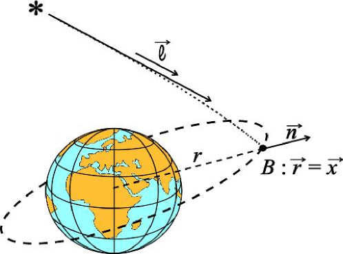
Figure 1: The deflection of light.

In space time, the direction of the light from the star is given by the 4-vector $L_{\alpha}=\left\{1,\;\dfrac{\partial_{k}\,\varphi}{\partial_{0}\,\varphi}\right\}$ where $\varphi$ is the phase of the light. In order to calculate the phase $\varphi(t,x^{k})$ at point $\left\{x^{k}\right\}$ and time $t$ we use the method which is summarized in annex A Linet and Tourrenc (1976).

The monopolar term of the Newtonian potential gives

$$L_{\alpha}=\left\{1,\;-\ell^{k}+\left(1+\gamma\right)\dfrac{M_{\oplus}}{r}\dfrac{n^{k}-\ell^{k}}{1-\vec{n}\cdot\vec{\ell}}\right\}$$ (10)

where $\overrightarrow{\ell}$ is the unitary vector of figure 1 and $\overrightarrow{n}=\overrightarrow{r}/r$ .

Several contributions must be added to the expression (10).

$$L_{\alpha}=\left\{1,\;-\ell^{k}+\left(1+\gamma\right)\dfrac{M}{r}\dfrac{n^{k}-\ell^{k}}{1-\vec{n}\cdot\vec{\ell}}+\delta\ell^{k}+\delta L^{k}\right\}$$

$\bullet\qquad$The term $\delta\ell^{k}$ is due to the quadrupolar term of the Earth. We give its value in appendix A. Its order of magnitude is $J_{2}O_{2}\sim 10^{-3}O_{2}$ when $\overrightarrow{\ell}$ is nearly orthogonal to the plane of the orbit.

$\bullet\qquad$The term due to $\dfrac{1}{2}\alpha_{1}U\,w^{k},$ a part of $g_{0k}$ in the metric (2), results in the modification $M_{\oplus}\rightarrow M=M_{\oplus}\left(1-\dfrac{\alpha_{1}\,\vec{w}\cdot\vec{\ell}}{2\left(1+\gamma\right)}\right).$ The demonstration is straight forward.

$\bullet\qquad$The contribution due to the rotation of the Earth has already been considered in the literature (Ibáñez (1983)). Since it is proportional to the ratio of the angular momentum and the square of $r$, it is negligible. The same conclusion holds for the term $\Delta$ in expression (1).

$\bullet\qquad$The Sun, the Moon and the other planets, give a contribution due to $U_{\ast}$ in (1); it varies slowly with the time and it is negligible, especially within the framework of a Fourier analysis at a much higher frequency.

For the observer $O,$ the space direction of the light is the four vector $\lambda^{\alpha}=L^{\alpha}-L_{\beta}\,u^{\beta}\,u^{\alpha}.$ The components of $\lambda^{\alpha}$ relatively to the tetrad $e_{\hat{\alpha}}^{\beta}$ are $\lambda_{\hat{\alpha}}=e_{\hat{\alpha}}^{\beta}\lambda_{\beta}.$

$$\lambda^{\hat{k}}=-\lambda_{\hat{k}}=-L_{\alpha}e_{\hat{k}}^{\alpha}\;,\;\;\lambda^{\hat{0}}=-\lambda_{\hat{0}}=0$$

In order to calculate $\lambda^{\hat{k}},$ we use the expression (6) for the tetrad. We normalize $\vec{\lambda},$ i.e. we define $\vec{\Lambda}=\Lambda\,\vec{\lambda}$ such as $-\Lambda_{\alpha}\Lambda^{\alpha}=\vec{\Lambda}\cdot\vec{\Lambda}=1.$ The tetrad (6) is especially useful to catch the orders of magnitude of the various terms involved. However it is not the comoving tetrad that we are looking for because the telescope that points towards the far away star rotates relatively to this tetrad. The angular velocity of the telescope relatively to $\left\{e_{\hat{k}}^{\alpha}\right\}$ is $\vec{\Omega}_{\ast}=\vec{\Lambda}\wedge\dfrac{d\vec{\Lambda}}{dt}.$ Straightforward calculations give

$$\Lambda^{\hat{k}} = \ell^{k}\,\left(1+\vec{\ell}\cdot\vec{v}-\dfrac{1}{2}\vec{v}^{\,2}+\left(\vec{\ell}\cdot\vec{v}\right)^{2}\right.$$

$$\left.+\left(1+\gamma\right)\dfrac{M}{r}\dfrac{\vec{n}\cdot\vec{\ell}}{1-\vec{n}\cdot\vec{\ell}}-\vec{\ell}\cdot\left(\delta\vec{\ell}+\delta\vec{L}\right)\right)$$

$$-v^{k}\,\left(1+\dfrac{1}{2}\left(\vec{\ell}\cdot\vec{v}\right)\right)-n^{k}\dfrac{M}{r}\dfrac{1+\gamma}{1-\vec{n}\cdot\vec{\ell}}+\delta\vec{\ell}+\delta\vec{L}+O_{3}$$

and

$$\left(\vec{\Omega}_{\ast}\right)^{\hat{k}} = -\left(\vec{\ell}\wedge\dfrac{d\vec{v}}{dt}\right)^{k}+\left(\vec{v}\wedge\dfrac{d\vec{v}}{dt}\right)^{k}$$

$$-\dfrac{3}{2}\left(\vec{\ell}\cdot\vec{v}\right)\left(\vec{\ell}\wedge\dfrac{d\vec{v}}{dt}\right)^{k}+\dfrac{1}{2}\left(\vec{\ell}\cdot\dfrac{d\vec{v}}{dt}\right)\left(\vec{\ell}\wedge\vec{v}\right)^{k}$$

$$-\dfrac{M}{r^{2}}\dfrac{1+\gamma}{1-\vec{n}\cdot\vec{\ell}}\left(\left(\vec{\ell}\wedge\vec{v}\right)^{k}+\left(\vec{\ell}\wedge\vec{n}\right)^{k}\;\left[\dfrac{\vec{\ell}\cdot\vec{v}\;-\vec{n}\cdot\vec{v}}{1-\vec{n}\cdot\vec{\ell}}-\vec{n}\cdot\vec{v}\right]\right)$$

$$+\left(\vec{\ell}\wedge\dfrac{d\delta\vec{\ell}}{dt}\right)^{k}+\dfrac{1}{r}\times O_{4}$$

Let us notice that we neglect the terms of order $\dfrac{1}{r}\times O_{4}$, which are much smaller than the Lense-Thirring angular velocity ($\sim 750\,O_{4}\times\dfrac{1}{r}).$

Now we introduce the tetrad $u_{\left(\sigma\right)}^{\alpha}$ which is obtained from $e_{\hat{\rho}}^{\alpha}$ through a pure space rotation (i.e. $u_{\left(0\right)}^{\alpha}=e_{\hat{0}}^{\alpha}=u^{\alpha})$ and whose vector $u_{\left(1\right)}^{\alpha}$ points towards the far away star ($u_{\left(1\right)}^{\alpha}=-\Lambda^{\alpha})$. The rotation of the tetrad $\left\{u_{\left(\sigma\right)}^{\alpha}\right\}$ relatively to $\left\{e_{\hat{\rho}}^{\alpha}\right\}$ is characterized by the most general angular velocity $\vec{\Omega}_{u/e}=\vec{\Omega}_{\ast}-\varpi\vec{\Lambda}$ where $-\varpi\vec{\Lambda}$ is an arbitrary angular velocity around the apparent direction of the star.

IV The local metric in the satellite

IV.1 The relevant terms

Now we need to calculate the NiZiLi metric associated to the tetrad $u_{\left(\sigma\right)}^{\alpha}$. We limit the accuracy of our development to a few tens per cent in order to take advantage of important simplifications.

Let us assume that the fundamental element is known :

$$ds^{2}=\left(1+K_{\left(0\right)\left(0\right)}\right)dT^{2}+2K_{\left(0\right)\left(k\right)}dTdX^{\left(k\right)}+\left(\eta_{\left(k\right)\left(j\right)}+K_{\left(k\right)\left(j\right)}\right)dX^{\left(k\right)}dX^{\left(j\right)}$$

We want to calculate the effect of $K_{\left(\alpha\right)\left(\beta\right)}$ on the atom interferometer in the satellite. In order to use the method summarized in the appendix A we calculate the quantity $\Psi$ which gives the physical quantities that one can measure :

$$\Psi=K_{\left(0\right)\left(0\right)}+2K_{\left(0\right)\left(k\right)}v_{g}^{\left(k\right)}+K_{\left(k\right)\left(j\right)}v_{g}^{\left(k\right)}v_{g}^{\left(j\right)}$$ (12)

where $v_{g}^{\left(k\right)}$ is the velocity of the atoms (i.e. the unperturbed group velocity).

We are dealing with slow cold atoms, therefore $v_{g}\sim\eta O_{1}$ with $\eta<<1$ (we can take the value $\eta\sim O_{1}$ valid for current experiments). In $\Psi,$ the Lense-Thirring term arises from $2K_{\left(0\right)\left(k\right)}v_{g}^{\left(k\right)};$ it is of order of $2\dfrac{J}{r^{3}}Xv_{g}\sim 1500\,\eta\varepsilon O_{6}.$ If the expansion of $K_{\left(0\right)\left(0\right)}$ is limited to order $\varepsilon^{2}O_{6},$ the accuracy is of order $\dfrac{\varepsilon}{1500\eta}\sim 13\%$ with $v_{g}\simeq 20\,{\rm cm}\cdot{\rm s}^{-1}.$

In the case that we consider, the following orders of magnitude hold true : $\varepsilon\sim\sqrt{O_{1}}=O_{1/2}$ and $\eta\sim O_{1}.$ Therefore, it is not necessary to consider terms smaller than $O_{7}\sim\varepsilon^{2}\,O_{6}$ in $K_{\left(0\right)\left(0\right)},$ smaller than $O_{5}$ in $K_{\left(0\right)\left(k\right)}$ and smaller than $O_{3}$ in $K_{\left(k\right)\left(j\right)}.$ The same relations hold in the coordinate system associated to the tetrad $\left\{u_{\left(\sigma\right)}^{\alpha}\right\}$ as well as $\left\{e_{\hat{\rho}}^{\alpha}\right\}$ because both are next to each other.

It can be proved that in the expression 1 the time can be considered as a parameter and that, within the present approximations, it is not necessary to consider time derivative in the expression II.4. Therefore one obtains

$$G_{\hat{0}\hat{0}} = 1+2\,\vec{a}\cdot\vec{X}-\hat{U},_{\hat{k}\hat{\jmath}}\,X^{\hat{k}}X^{\hat{\jmath}}-\dfrac{1}{3}\hat{U},_{\hat{k}\hat{\jmath}\hat{\ell}}\,X^{\hat{k}}X^{\hat{\jmath}}X^{\hat{\ell}}+\varepsilon^{2}\,O_{6}$$

$$G_{\hat{0}\hat{m}} = -\left\{\vec{\Omega}_{0}\wedge\vec{X}\right\}^{\hat{m}}+\varepsilon^{2}\,O_{5}{\rm and\ }G_{\hat{n}\hat{m}}=\eta_{\hat{n}\hat{m}}+\varepsilon^{2}O_{4}$$

where $\vec{\Omega}_{0}$ is given above (see expression 7) while the expressions such as $\hat{U},_{\hat{k}\hat{\jmath}}$ are nothing but $\left(U_{,mn}\,e_{\hat{k}}^{m}e_{\hat{\jmath}}^{n}\right)_{O}.$ The position of the observer changes with time, therefore this quantity is a function of $T.$

In $G_{\hat{0}\hat{0}},$ such an expansion is limited to the terms of order of $\varepsilon^{2}\,O_{6},$ thus the approximation $e_{\hat{k}}^{m}=\delta_{\hat{k}}^{m}$ is valid and $\hat{U},_{\hat{k}\hat{\jmath}}\simeq\left(U_{,kj}\right)_{O}.$ For $\vec{\Omega}_{0}$ the same holds true : $\left(\vec{\Omega}_{0}\right)^{\hat{k}}\simeq\left(\vec{\Omega}_{0}\right)^{k}$ (see expression 7). Therefore, one can identify the space vectors $\overrightarrow{e}_{\hat{k}}$ of the tetrad and the space vectors $\overrightarrow{\partial}_{k}$ of the natural basis associated to the geocentric coordinates. This would not be valid with an higher accuracy where terms smaller than $\varepsilon^{2}\,O_{6}$ are considered.

The change of the tetrad $u_{\left(\sigma\right)}^{\alpha}\longleftrightarrow e_{\hat{\rho}}^{\alpha}$ is just an ordinary change of basis in the space of the observer $O.$ In this transformation, $dT,$ $G_{\hat{0}\hat{0}}=G_{\left(0\right)\left(0\right)}$, $G_{\hat{0}\hat{m}}dX^{\hat{m}}=G_{\left(0\right)\left(k\right)}dX^{\left(k\right)}$ and $G_{\hat{n}\hat{m}}dX^{\hat{m}}dX^{\hat{n}}=G_{\left(j\right)\left(k\right)}dX^{\left(j\right)}X^{\left(k\right)}$ behave as scalars.

As a consequence, we put forward that within the required accuracy, it is possible to give a simple description of the Hyper project with the Newtonian concept of space. It is now straightforward to calculate $\Psi$ :

$$\Psi = 2\,\vec{a}\cdot\vec{X}-\hat{U},_{\left(k\right)\left(j\right)}\,X^{\left(k\right)}X^{\left(j\right)}-\dfrac{1}{3}\hat{U},_{\left(k\right)\left(j\right)\left(\ell\right)}\,X^{\left(k\right)}X^{\left(j\right)}X^{\left(\ell\right)}$$

$$-2\underset{\left(k\right)}{\sum}\left\{\left(\vec{\Omega}_{0}+\vec{\Omega}_{\ast}\right)\wedge\vec{X}\right\}^{\left(k\right)}v_{g}^{\;\left(k\right)}+\varepsilon^{2}O_{6}$$

Now we assume that any quantity can be known with an accuracy $\mu$ of order of $10^{-5}\lesssim O_{1}.$ It means that the geometry of the experimental device is known with an accuracy of order of $10{\rm\mu m}.$ The position of the point $O$ on the trajectory of the satellite is known with an accuracy better than $70\,{\rm m},$ the eccentricity can be controlled to be smaller than $O_{1},$ etc.

We consider that $\Psi$ is the amount of two terms, $\Psi_{k}$ and $\Psi_{u}~{}:$ the term $\Psi_{k}$ can be modelled with the required accuracy while $\Psi_{u}$ is unknown. The terms $\Psi_{k}$ fulfills the condition $\mu$$\times\Psi_{k}\lesssim\varepsilon^{2}\,O_{6}.$ With the previous orders of magnitude ($\varepsilon\sim O_{1/2}\sim 5\,10^{-3}$ and $\mu$$\,\sim O_{1}\sim 2.5\,10^{-5})$ one finds

$$\Psi_{u}=2\,\vec{a}\cdot\vec{X}-\hat{U},_{\left(k\right)\left(j\right)}\,X^{\left(k\right)}X^{\left(j\right)}-2\left\{\vec{\Omega}\wedge\vec{X}\right\}\cdot\overrightarrow{v}_{g}+\varepsilon^{2}O_{6}/{\mu}$$

$\hat{U},_{\left(k\right)\left(j\right)}$ is obtained from the expression 1 of $U$ limited to the monopolar and the quadrupolar terms and

$$\left(\vec{\Omega}\right)^{\left(k\right)}=\left(\vec{\Omega}_{LT}-\varpi\overrightarrow{\Lambda}-\overrightarrow{\Lambda}\wedge\dfrac{d\overrightarrow{v}}{dt}\right)^{\left(k\right)}+\dfrac{O_{3}}{r}$$

where $\vec{\Omega}_{LT}$ is obtained from 8 and $\dfrac{d\overrightarrow{v}}{dt}\simeq\overrightarrow{a}-\overrightarrow{\nabla}U\simeq\overrightarrow{a}+\dfrac{M_{\oplus}}{r^{2}}\overrightarrow{n}.$

IV.2 Calculation of $\Psi_{u}$

We consider that the motion of the satellite is a Newtonian motion which takes place in the $\left(x,y\right)$-plane while the vector $\overrightarrow{\ell}$ lies in the $\left(x,z\right)$-plane. We assume that the eccentricity, $e,$ does not exceed $O_{1}$.

We define

$$\vec{J} = J_{x}\,\vec{e}_{\hat{1}}+J_{y}\,\vec{e}_{\hat{2}}+J_{z}\,\vec{e}_{\hat{3}}\;,\;\;\vec{n}=\cos\theta\,\vec{e}_{\hat{1}}+\sin\theta\,\vec{e}_{\hat{2}}$$

$$-\vec{\ell} = \cos\alpha\,\vec{e}_{\hat{1}}+\sin\alpha\,\vec{e}_{\hat{3}}\;,\;\;\vec{w}=w_{x}\,\vec{e}_{\hat{1}}+w_{y}\,\vec{e}_{\hat{2}}+w_{z}\,\vec{e}_{\hat{3}}$$

$\vec{J},$ $\vec{\ell}$ and $\vec{w}$ are constant vectors. The angle $\theta$ and the distance $r$ depend on the time $T$.

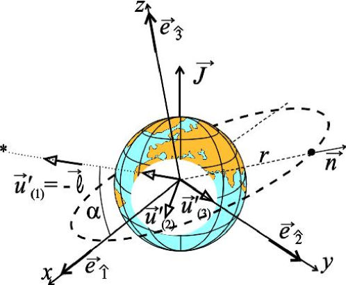
Figure 2: The satellite and the fixed star.

First we define the special triad $\vec{u}_{(n)}^{\prime}$ :

$$\vec{u}_{(1)}^{\prime}=\cos\alpha\,\overrightarrow{e}_{\hat{1}}+\sin\alpha\overrightarrow{e}_{\hat{3}},\;\;\vec{u}_{(2)}^{\prime}=\sin\alpha\,\overrightarrow{e}_{\hat{1}}-\cos\alpha\overrightarrow{e}_{\hat{3}},\;\;\vec{u}_{(3)}^{\prime}=\overrightarrow{e}_{\hat{2}}$$

Let us outline that we have defined $\left(\vec{u}_{(1)}^{\prime}\right)^{\hat{k}}=-\left(\vec{\Lambda}\right)^{\hat{k}}+O_{1}$. Then, in order to obtain the final tetrad $u_{\left(\sigma\right)}^{\alpha},$ we perform an arbitrary rotation around $\vec{\Lambda}~{}:$

$$\vec{u}_{(1)}=-\vec{\Lambda}=\vec{u}_{(1)}^{\prime}+O_{1}$$

(13)

where $-\dfrac{d\sigma}{dT}=-\varpi$ is the angular velocity of the triad $\left\{\vec{u}_{(k)}\right\}$ relatively to $\left\{\vec{u}_{(k)}^{\prime}\right\}.$

We can now assume that the experimental set-up is comoving with the triad $\vec{u}_{(n)}$ whose vector $\vec{u}_{(1)}$ points towards the fixed star.

In order to calculate the quadrupolar term in $U,$ we define the unitary vector, $\overrightarrow{k}$ along the axi-symmetry axis. One obtains

$$U=\dfrac{M_{\oplus}}{r}-\dfrac{1}{2}J_{2}\dfrac{M_{\oplus}}{r}\left(\dfrac{R_{\oplus}}{r}\right)^{2}\left(3\,\left(\overrightarrow{k}\cdot\overrightarrow{n}\right)^{2}-1\right)$$

Therefore $\Psi_{u}$ reads

$$\begin{array}[]{ll|l}\Psi_{u}=&-2\left(\left(\dfrac{\vec{J}}{r^{3}}-\dfrac{3\left(\vec{J}\cdot\vec{n}\right)}{r^{3}}\vec{n}+\dfrac{\alpha_{1}\;M_{\oplus}}{4\,r^{2}}\,\vec{n}\wedge\vec{w}\right)\wedge\vec{x}\right)\cdot\vec{v}_{g}&A\\ &-2\varpi\,\left(\vec{u}_{(1)}\wedge\vec{x}\right)\cdot\vec{v}_{g}&B\\ &-2\dfrac{M_{\oplus}}{r^{2}}\left(\left(\vec{u}_{(1)}\wedge\vec{n}\right)\wedge\vec{x}\right)\cdot\vec{v}_{g}+2\left(\left(\vec{u}_{(1)}\wedge\vec{a}\right)\wedge\vec{x}\right)\cdot\vec{v}_{g}&C\\ &+\dfrac{M_{\oplus}}{r^{3}}\left(\vec{x}^{2}-3\,\left(\vec{n}\cdot\vec{x}\right)^{2}\right)+\dfrac{3}{2}J_{2}\dfrac{M_{\oplus}}{r^{3}}\left(\dfrac{R_{\oplus}}{r}\right)^{2}Q&D\\ &+2\,\vec{a}\cdot\vec{x}&E\end{array}$$ (14)

with

$$Q = \left(1-5\,\left(\overrightarrow{k}\cdot\overrightarrow{n}\right)^{2}\right)\overrightarrow{X}^{\,2}-20\left(\overrightarrow{k}\cdot\overrightarrow{n}\right)\left(\overrightarrow{n}\cdot\overrightarrow{X}\right)\left(\overrightarrow{k}\cdot\overrightarrow{X}\right)$$

$$+5\left(7\,\left(\overrightarrow{k}\cdot\overrightarrow{n}\right)^{2}-3\right)\left(\overrightarrow{n}\cdot\overrightarrow{X}\right)^{2}+2\left(\overrightarrow{k}\cdot\overrightarrow{X}\right)^{2}$$

and

$$\overrightarrow{J} = J\,\overrightarrow{k}$$

In $\Psi_{u},$ the two terms $2\,\vec{a}\cdot\vec{X}$ and $-2\varpi\,\left(\vec{u}_{(1)}\wedge\overrightarrow{X}\right)\cdot\vec{v}_{g}$ are directly calculated in the local coordinates associated to the tetrad $u_{\left(\sigma\right)}^{\alpha}$ moreover, to calculate the other quantities where $\vec{n}$ is involved, one can drop the terms of order $O_{1}$ in the expression of $\vec{u}_{(1)}.$ The reason is that the quantities that we drop are either negligible or included in $\Psi_{k}.$ Therefore, it is clear that we can consider the space as the ordinary space of Newtonian physics and that the usual formulae to change the basis $\overrightarrow{\partial}_{k}$ into $\overrightarrow{e}_{\hat{k}}$ or $\overrightarrow{u}_{\left(k\right)}$are valid.

In (14), the terms of lines $A,$ $B$ and $C$ are due to various rotations : respectively the Lense-Thirring rotation, the spin around the view line of the star and the aberration. The term of line $D$ gives the gravitational tidal effects (which are mainly due to the Earth) and the last term (line $E)$ corresponds to some residual acceleration due to the fact that point $O$ is not exactly in free fall.

It is now possible to calculate explicitly $\Psi_{u}$ with the coordinates $X^{(k)},$ comoving with the experimental set-up .

V The experimental set-up

V.1 The atomic Sagnac unit

An atomic Sagnac unit (ASU) is made of two counter-propagating atom interferometers which discriminate between rotation and acceleration (see figure 3-$a$).

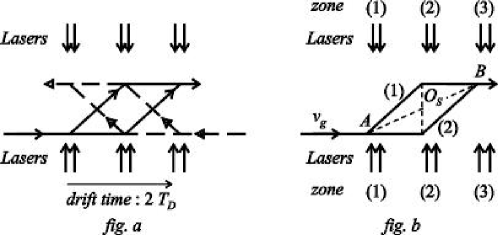
Figure 3: An atomic Sagnac unit (ASU).

Each interferometer is a so-called Ramsey-Bordé interferometer with a Mach-Zehnder geometry ( figure 3-$b$). The atomic beam from a magneto-optical trap interacts three times with a laser field. In the first interaction zone the atomic beam is split coherently, by a Raman effect, into two beams which are redirected and recombined in the second and the third interaction zone.

The mass of the atom depends on its internal state, therefore it is not a constant along the different paths. However, the change of the mass is very small; it leads to negligible corrections on the main effects which is already very small. Considering cesium, we assume that the mass of the atom is a constant $m=133\times 1.66\times 10^{-27}=2.2\times 10^{-25}\,{\rm kg}.$

In this case the wave length of the lasers is $\lambda=850\,{\rm nm}.$ The momentum transferred to the atom during the interaction is $\dfrac{4\pi\hbar}{\lambda}.$ The recoil of the atom results in a Sagnac loop which permits to measure the angular velocity of the set-up relatively to a local inertial frame. The device is also sensitive to the accelerations.

One can easily imagine that there are many difficulties to overcome if the Lense-Thirring effect is to be observed. In particular, the geometrical constraints appear to be crucial. In an ideal set-up the two interferometers are identical coplanar parallelograms with their center $O_{S}$ and $O_{S}^{\prime}$ at the same point. One can consider several perturbation to this geometrical scheme.

1. A shift : $O_{S}$ and $O_{S}^{\prime}$ are no longer at the same point;

2. A tilt : The plane of the two interferometers are now different;

3. A deformations : the interferometers are no longer identical lozenges, they are no longer parallelogram, even not plane interferometers.

The geometry of the device is fully determine by the interaction between the initial atomic beam and the lasers ; moreover the geometrical description is already an idealized model ; Therefore a full treatment of the atom-laser interaction in a gravitational field is obviously necessary to study the response of the ASU (see Antoine and Bordé (2003)). However the geometrical model is useful to give a physical intuition of the phenomena. In this context we study here the effect of a shift on the signal.

In the sequel we consider an ideal set-up where the beams are perfectly coherent and perfectly parallel, point $O_{S}$ being a perfect center of symmetry for the atomic paths. We assume also that the two counter-propagating atom interferometers are identical and located in the same plane but that the separation of their center of symmetry, $O_{S}$ and $O_{S}^{\prime},$ is the vector $\vec{\delta}=\overrightarrow{O_{S}O_{S}^{\prime}}.$

We will assume that the velocity, $v_{g},$ of the atoms is of the order of $20\,{\rm cm}\cdot{\rm s}^{-1}$ and that the size of the ASU is of order of $60\,{\rm cm},$ therefore the drift time is $2T_{D}\sim 3\,{\rm s}.$

V.2 The phase differences

The configuration which is presently considered in the Hyper project is on figure 4.

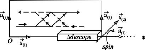
Figure 4: The experimental set-up.

We consider one among the four interferometers of the device above. Using the results of appendix A, we obtain the phase difference that we want to measure:

$$\delta\varphi=\dfrac{\omega}{2}\int_{t-2T_{D}/(2)}^{t}\psi\,(t^{\prime})\;dt^{\prime}-\dfrac{\omega}{2}\int_{t-2T_{D}/\left(1\right)}^{t}\psi\,(t^{\prime})\;dt^{\prime}$$ (15)

The integrals are performed along path (2) and (1) of figure 3-$b$. The ”angular frequency” $\omega$ is defined as $\dfrac{m\,c^{2}}{\hbar}.$

We consider that the origin is the center of symmetry $O_{S}.$ The coordinates are $\overrightarrow{X}=\left\{X^{\left(k\right)}\right\}.$ We define $\vec{v}_{g}=\dfrac{d\overrightarrow{X}}{dt}$ as the unperturbed group velocity of the atoms

We make use of the properties of the Newtonian trajectory :

$$r=\dfrac{r_{0}}{1+e\cos\theta},\;\vec{n}=\cos\theta\,\vec{e}_{\hat{1}}+\sin\theta\,\vec{e}_{\hat{2}},\;\dfrac{d\theta}{dT}=\Omega_{S}\left(1+e\cos\theta\right)^{2}$$

with $\Omega_{S}=\dfrac{M_{\oplus}}{r_{0}^{\;2}}.$ We consider the case where the ellipticity, $e,$ is much smaller than unity. Therefore, up to first order relatively to $e,$ one obtains

$$\dfrac{1}{r}=\dfrac{1}{r_{0}}\left(1+e\cos\theta\right)\;,\;\;\theta\simeq\Omega_{S}\,t+\theta_{0}+e\sin\left(\Omega_{S}\,t+\theta_{0}\right)$$

We assume $e\lesssim O_{1},$ therefore in the expression (14) of $\Psi_{u}$ one can assume that $r=r_{0}$ is a constant because the corrections due to the eccentricity are included in $\Psi_{k}.$

During the flight time of an atom, one cannot consider that $\overrightarrow{n}$ remains a constant in expression (14). One can consider that the coordinate, $X=X^{\left(1\right)}$ of the atom is a function of the time: $X=v_{g}\left(T-T_{0}\right).$ Then $\overrightarrow{n}=\overrightarrow{n}_{0}+\delta\overrightarrow{n}$ where $\overrightarrow{n}_{0}$ depends on $T_{0}$ only and $\delta\overrightarrow{n}$ on $T_{0}$ and $X/v_{g}.$ Therefore, in expression (15), we expand the different terms relatively to $X/v_{g}.$ Any of the correction can be included in $\Psi_{k}$ except the first order correction, $\delta\psi_{D},$ of the first term in line $D.$

$$\delta\psi_{D}=-\dfrac{6M_{\oplus}}{r^{4}}\left(\overrightarrow{x}\cdot\dfrac{\overrightarrow{v}}{v_{g}}\right)\left(\overrightarrow{x}\cdot\overrightarrow{n}_{0}\right)x$$

The result of the integration is now straightforward. We change the notation : $\overrightarrow{n}_{0}\rightarrow\overrightarrow{n}$ and $T_{0}\rightarrow T$. In usual units one finds :

$$\delta\varphi=$$

where $S=\dfrac{4\pi\hbar}{\lambda\,m}v_{g}T_{D}^{\;2}$ is the area of the Sagnac loop.

Line $B$ in (14) gives no contribution because $\overrightarrow{X},$ $\vec{u}_{(1)}$ and $\overrightarrow{v}_{g}$ are in the same plane. The quadratic terms have disappeared because $O_{S}$ is a center of symmetry.

The two interferometers of the same ASU are assumed to lie in the same plane but not necessarily with their center of symmetry $O_{S}$ and $O_{S}^{\prime}$ at the same point. Therefore adding and subtracting the phase differences delivered by the two interferometers one finds the two basic quantities which are measured by the set-up i.e. :

$${\mu}_{1} = \dfrac{1}{2}\left(\delta\varphi^{\prime}-\delta\varphi\right)=\dfrac{8\pi}{\lambda}\left(cT_{D}\right)^{2}\left\{\dfrac{M_{\oplus}}{r^{2}}\,\vec{u}_{(3)}\cdot\vec{n}+\vec{u}_{(3)}\cdot\overrightarrow{a}+\vec{\Omega}_{LT}\cdot\vec{u}_{(2)}\right\}\dfrac{v_{g}}{c}$$

$$+\dfrac{2\pi\left(cT_{D}\right)^{2}}{\lambda}\left\{\left(\dfrac{\vec{a}_{O_{S}}}{c^{2}}-\dfrac{\,\vec{a}_{O_{S}^{\prime}}}{c^{2}}\right)\cdot\vec{u}_{(3)}\right\}$$

$$-\dfrac{mc}{2\hbar}\dfrac{\left(cT_{D}\right)^{2}S}{r^{3}}\dfrac{M_{\oplus}}{r}\left(\left(\vec{u}_{(1)}\cdot\vec{n}\right)\left(\vec{u}_{(3)}\cdot\dfrac{\overrightarrow{v}}{c}\right)+\left(\vec{u}_{(3)}\cdot\vec{n}\right)\left(\vec{u}_{(1)}\cdot\dfrac{\overrightarrow{v}}{c}\right)\right)$$

$${\mu}_{2} = \dfrac{1}{2}\left(\delta\varphi^{\prime}+\delta\varphi\right)=-\dfrac{4\pi\left(cT_{D}\right)^{2}}{\lambda}\left\{\dfrac{\overrightarrow{a}}{c^{2}}\cdot\vec{u}_{(3)}\right\}$$

where now $\overrightarrow{a}=\vec{a}_{O_{S}}+\,\vec{a}_{O_{S}^{\prime}}.$ In the expression above, we have dropped the term $-\dfrac{mc}{2\,\hbar r}S\,\dfrac{\left(cT_{D}\right)^{2}}{r^{2}}\dfrac{M_{\oplus}}{r}\,\dfrac{4\pi\hbar}{\lambda mv_{g}}\left(\vec{u}_{(3)}\cdot\vec{n}\right)\left(\vec{u}_{(3)}\cdot\overrightarrow{v}\right)$ because it can be included in $\Psi_{k}.$

$a_{O_{S}}^{\;\left(k\right)}u_{\left(k\right)}^{\alpha}$ is the 4-acceleration of point $O_{S}.$ Therefore, one calculates $\left(\vec{a}_{O_{S}}-\,\vec{a}_{O_{S}^{\prime}}\right)\cdot\vec{u}_{(3)}=-\hat{U}_{,\left(k\right)\left(3\right)}x_{O_{S}}^{\;\left(k\right)}$ where we have dropped the non significant terms which can be included in $\Psi_{k}.$

The quantities which can be measured are

$$\mu_{1}+2v_{g}\mu_{2} = \dfrac{8\pi}{\lambda}\left(cT_{D}\right)^{2}\left\{\dfrac{M_{\oplus}}{r^{2}}\vec{u}_{(3)}\cdot\vec{n}+\vec{\Omega}_{LT}\cdot\vec{u}_{(2)}\right\}\dfrac{v_{g}}{c}$$

$$-\dfrac{2\pi\left(cT_{D}\right)^{2}}{\lambda r}\dfrac{M_{\oplus}}{r}\left(\vec{u}_{(3)}\cdot\dfrac{\overrightarrow{\delta}}{r}-3\left(\vec{n}\cdot\vec{u}_{(3)}\right)\left(\vec{n}\cdot\dfrac{\overrightarrow{\delta}}{r}\right)\right)$$

$$-\dfrac{2\pi}{\lambda}\left(cT_{D}\right)^{2}\left(\dfrac{v_{g}T_{D}}{r}\right)^{2}\dfrac{M_{\oplus}}{r^{2}}\left\{\left(\vec{u}_{(1)}\cdot\vec{n}\right)\left(\vec{u}_{(3)}\cdot\dfrac{\overrightarrow{v}}{c}\right)+\left(\vec{u}_{(3)}\cdot\vec{n}\right)\left(\vec{u}_{(1)}\cdot\dfrac{\overrightarrow{v}}{c}\right)\right\}$$

$${\mu}_{2} = \dfrac{1}{2}\left(\delta\varphi^{\prime}+\delta\varphi\right)=-\dfrac{4\pi\left(cT_{D}\right)^{2}}{\lambda}\left\{\dfrac{\overrightarrow{a}}{c^{2}}\cdot\vec{u}_{(3)}\right\}$$

where $\overrightarrow{\delta}=\overrightarrow{x}_{O_{S}^{\prime}}-\overrightarrow{x}_{O_{S}}.$

V.3 Discussion

We define the projection, $\overrightarrow{J}_{\shortparallel}$ of $\overrightarrow{J}$ on the plane of the orbit : $\overrightarrow{J}_{\shortparallel}=J_{\shortparallel}\left(\cos\theta_{J}\;\overrightarrow{e}_{\hat{1}}+\sin\theta_{J}\;\overrightarrow{e}_{\hat{2}}\right)$ and $\overrightarrow{w}_{\shortparallel}=w_{\shortparallel}\left(\cos\theta_{w}\;\overrightarrow{e}_{\hat{1}}+\sin\theta_{w}\;\overrightarrow{e}_{\hat{2}}\right).$ Going back to usual units (with $M_{\oplus}\simeq 4.4\,{\rm mm}$ and $J\simeq 145\,{\rm cm}^{2})$ we obtain

$${\mu}_{1}+2\dfrac{v_{g}}{c}{\mu}_{2} = \dfrac{2\pi\left(cT_{D}\right)^{2}}{\lambda r_{0}}\times\left\{K_{0}+K_{\sigma}+K_{2\sigma}+K_{2\theta}\right.$$

$$\left.+K_{\theta-\sigma}+K_{\theta+\sigma}+K_{2\theta-\sigma}+K_{2\theta+\sigma}+K_{2\theta-2\sigma}+K_{2\theta+2\sigma}\right\}$$

with

$$K_{0} = \dfrac{M_{\oplus}}{4\,r_{0}}\left(3\sin^{2}\alpha-1\right)\times\dfrac{\delta^{(3)}}{r_{0}}$$

$$K_{\sigma} = \dfrac{v_{g}}{c}\left\{\left[\left(1-\sin\alpha\right)\cos\left(\sigma+\theta_{J}\right)-\left(1+\sin\alpha\right)\cos\left(\sigma-\theta_{J}\right)\right]\times\dfrac{J_{\shortparallel}}{r_{0}^{\;2}}\right.$$

$$\left.-4\cos\alpha\,\cos\sigma\times\dfrac{J^{\hat{3}}}{r_{0}^{\;2}}\right\}-\dfrac{3M_{\oplus}}{2r_{0}}\cos\alpha\sin\alpha\sin\sigma\times\dfrac{\delta^{\left(1\right)}}{r_{0}}$$

$$K_{2\sigma} = \dfrac{3M_{\oplus}}{4r_{0}}\left(1-\sin^{2}\alpha\right)\,\left[\sin\left(2\sigma\right)\times\dfrac{\delta^{(2)}}{r_{0}}+\cos\left(2\sigma\right)\times\dfrac{\delta^{(3)}}{r_{0}}\right]$$

$$K_{2\theta} = -\dfrac{3M_{\oplus}}{4r_{0}}\left(1-\sin^{2}\alpha\right)\,\cos\left(2\theta\right)\times\dfrac{\delta^{\left(3\right)}}{r_{0}}$$

$$K_{\theta-\sigma} = \dfrac{M_{\oplus}}{r_{0}}\dfrac{v_{g}}{c}\times\left\{-2\left(1+\sin\alpha\right)\,\sin\left(\theta-\sigma\right)\right.$$

$$\left.+\dfrac{\alpha_{1}}{2}\cos\alpha\,\sin\left(\theta-\sigma-\theta_{w}\right)\times\dfrac{w_{\shortparallel}}{c}\right.$$

$$\left.+\dfrac{\alpha_{1}}{2}\left(1+\sin\alpha\right)\sin\left(\theta-\sigma\right)\times\dfrac{w^{\hat{3}}}{c}\right\}$$

$$K_{\theta+\sigma} = \dfrac{M_{\oplus}}{r_{0}}\dfrac{v_{g}}{c}\times\left\{-2\left(1-\sin\alpha\right)\,\sin\left(\theta+\sigma\right)\right.$$

$$\left.+\dfrac{\alpha_{1}}{2}\cos\alpha\,\sin\left(\theta+\sigma-\theta_{w}\right)\times\dfrac{w_{\shortparallel}}{c}\right.$$

$$\left.-\dfrac{\alpha_{1}}{2}\left(1-\sin\alpha\right)\sin\left(\theta+\sigma\right)\times\dfrac{w^{\hat{3}}}{c}\right\}$$

$$K_{2\theta-\sigma} = -3\dfrac{v_{g}}{c}\left(1+\sin\alpha\right)\cos\left(2\theta-\sigma-\theta_{J}\right)\times\dfrac{J_{\shortparallel}}{r_{0}^{\;2}}$$

$$+\dfrac{3M_{\oplus}}{4r_{0}}\cos\alpha\,\left(1+\sin\alpha\right)\sin\left(2\theta-\sigma\right)\times\dfrac{\delta^{\left(1\right)}}{r_{0}}$$

$$-\left(\dfrac{M_{\oplus}}{r_{0}}\right)^{3/2}\dfrac{cv_{g}T_{D}^{\;2}}{2\,r_{0}^{\;2}}\left(1+\sin\alpha\right)\cos\left(2\theta-\sigma\right)$$

$$K_{2\theta+\sigma} = 3\dfrac{v_{g}}{c}\left(1-\sin\alpha\right)\cos\left(2\theta+\sigma-\theta_{J}\right)\times\dfrac{J_{\shortparallel}}{r_{0}^{\;2}}$$

$$+\dfrac{3M_{\oplus}}{4r_{0}}\cos\alpha\,\left(1-\sin\alpha\right)\sin\left(2\theta+\sigma\right)\times\dfrac{\delta^{\left(1\right)}}{r_{0}}$$

$$-\left(\dfrac{M_{\oplus}}{r_{0}}\right)^{3/2}\dfrac{cv_{g}T_{D}^{\;2}}{2\,r_{0}^{\;2}}\left(1-\sin\alpha\right)\cos\left(2\theta+\sigma\right)$$

$$K_{2\theta-2\sigma} = \dfrac{3M_{\oplus}}{8\,r_{0}}\left(1+\sin\alpha\right)^{2}\left\{\sin\left(2\theta-2\sigma\right)\times\dfrac{\delta^{\left(2\right)}}{r_{0}}-\cos\left(2\theta-2\sigma\right)\times\dfrac{\delta^{\left(3\right)}}{r_{0}}\right\}$$

$$K_{2\theta+2\sigma} = -\dfrac{3M_{\oplus}}{8\,r_{0}}\left(1-\sin\alpha\right)^{2}\left\{\sin\left(2\theta+2\sigma\right)\times\dfrac{\delta^{\left(2\right)}}{r_{0}}+\cos\left(2\theta+2\sigma\right)\times\dfrac{\delta^{\left(3\right)}}{r_{0}}\right\}$$

Each of these terms, except $K_{0},$ has a specific frequency. These terms can be measured and distinguished from each other.

The Lense-Thirring effect due to the angular momentum of the Earth appears in the terms $K_{\sigma}$ and $K_{2\theta\pm\sigma}$ while the possible existence of a preferred frame appears in $K_{\theta\pm\sigma}$ which depends on the components of $\alpha_{1}\overrightarrow{w}.$

The signal due to the Lense-Thirring effect is associated with the signal due to $\delta^{\left(1\right)}.$ The two signals display the same order of magnitude when $\delta^{\left(1\right)}\sim 1\,{\rm nm}.$ Today, it seems impossible to achieve such a precision, this is the reason why $\delta^{\left(1\right)}$ should be calculated from the Fourier analysis of the signal itself, altogether with the angular momentum of the Earth, $\overrightarrow{J}$ and the velocity $\alpha_{1}\overrightarrow{w}.$

If the sensitivity to measure the Lense-Thirring effect with an accuracy of 20% is achieved, it should be possible to know $\alpha_{1}\overrightarrow{w}$ with an accuracy better than $10^{-7}.$ Considering that $\overrightarrow{w}$ is the velocity of the rest frame of the Universe ($\left\|\overrightarrow{w}\right\|\sim 10^{-3})$ it would give precision on $\alpha_{1}$ of order of $10^{-4}.$

The interest of the spin is obvious. If $\sigma=cte$ (no spin) the signal is the sum of two periodic signals with frequency $\nu_{O}$ and $2\nu_{O}$ where $\nu_{O}$ is the orbital frequency of the satellite ; therefore one ASU gives two informations (two functions of the time). When the satellite spins, we get 9 functions of the time $t.$ The information is much more important in this case.

VI Conclusion

In this paper we have sketched a method to take into account the residual gravitation in a nearly free falling satellite, namely the tidal and higher order effects. We have shown that these effects are not negligible in highly accurate experiments.

We have shown that many perturbations must be considered if one wants to observe the Lense-Thirring effect and we have exhibited the various terms that one needs to calculate in order to obtain the full signal.

Compared with GPB, the principle of the measure is not the same, the difficulties are quite different but the job is not easier. For instance, considering the quantities $K_{\sigma}$ or $K_{2\theta\pm\sigma}$ above, one can check that $\delta^{\left(1\right)}$ must remain smaller than $2\,{\rm nm}$ for the corresponding signal to remain smaller than the Lense-Thirring one. It does not seem that such a precision can be controlled in the construction of the experimental device itself. It is therefore necessary to measure $\delta^{\left(1\right)}$ with such an accuracy.

In the problem that we have considered, there are 9 unknown parameters : i) the three component of $\overrightarrow{J},$ ii) the three components of $\alpha_{1}\overrightarrow{w}$ and iii) the three components of $\overrightarrow{\delta}.$ On the other hand, the experimental set-up displays 9 periodic functions but the distribution of the unknown parameters among the 9 functions happen in such way that the four parameters $\overrightarrow{J}$ and $\delta^{(1)}$ are present in the 3 functions $K_{\sigma}$ or $K_{2\theta\pm\sigma}$ and the three parameters $\alpha_{1}\overrightarrow{w}$ in the two functions $K_{\theta\pm\sigma}$. Only the two parameters $\delta^{\left(2\right)}$ and $\delta^{\left(3\right)}$ are over determined by the four functions $K_{2\theta},$ $K_{2\sigma}$ and $K_{2\theta\pm 2\sigma}.$

Let us assume that $\theta$ and $\sigma$ are known function of the time (frequency and phase). This implies that in the geometric scheme that we have explored, one can determine 18 unknown parameters. Therefore $\overrightarrow{J},$ $\overrightarrow{\delta}$ and $\alpha_{1}\overrightarrow{w}$ can be known and the Lense-Thirring effect can be observed with an accuracy of a few tens percent. The same sensitivity on the phase difference of matter waves in the interferometers yields an accuracy of $10^{-7}$ on $\alpha_{1}\overrightarrow{w}$ which would increase our knowledge on $\alpha_{1}$ by one order of magnitude. This optimistic conclusion must be tempered with the remark that only the shift has been considered here while several other geometrical perturbations play their role. Moreover a crucial point is the knowledge of the phase of the various periodic functions $K$. The geometric scheme fails to describe the change of the phase of the atomic wave when it goes through the laser beam and we believe that the preceding conclusion holds only in the case where the change of the phase along the two paths differs by a constant.

As a conclusion, we put forward that only a more powerful model can answer the question of the theoretical feasibility. This model should take into account all the gravitational perturbations that we have outlined here and it should consider the interaction between laser fields and matter waves in more a realistic manner.

Appendix A The gravitational phase shifts

Let us assume that space time is quasi Minkowskian. Therefore, the metric is: $ds^{2}=\left(\eta_{\alpha\beta}+h_{\alpha\beta}\right)\,dx^{\alpha}dx^{\beta}$ with   $\left|h_{\alpha\beta}\right|<<1$.

Let us consider, at the eikonal approximation, a wave which propagates from the point $A$ to a point $B.$ The phase at point $A$ is known. It is $\varphi_{A}(t)=\omega t$ where $\omega$ is a constant and $t=x^{0}/c$ the time. The phase, $\varphi_{B}(t),$ at point $B$ is the amount of the unperturbed phase, $\overset{{\rm o}}{\varphi}_{B}(t),$ and the perturbation $\delta\varphi_{B}$ due to the term $h_{\alpha\beta}$ in the metric.

Two different cases are relevant for the problem that we study

1. Point $A$ is a far away, fixed, star. It is the source of a light wave. From the knowledge of $\varphi_{B}(t)$ at every point $B$ one can deduce the apparent direction of the star. Then it becomes possible to determine the vector $-L^{\alpha}$ which points towards $A.$

2. Point $A$ is the source of an atomic wave which enters a matter wave interferometer. At point $B$ interferences are observed on a detector (figure 3-$b$). The phases $\varphi_{B1}(t)$ and $\varphi_{B2}(t),$ of the waves which interfere at point $B$ depend on the path, $(1)$ or $(2)$, that each wave has followed. The response of the detector at point $B$ depends on the difference $\varphi_{B1}(t)-\varphi_{B2}(t).$ Therefore one can obtain the response of the interferometer once the phases $\varphi_{B1}(t)$ and $\varphi_{B2}(t)$ are known.

In order to calculate the phase $\varphi_{B}(t)$ at point $B$ and time $t$ we use the method developed in Linet and Tourrenc (1976). We summarize briefly the method for particles of mass $m$ (for the light $m=0).$

First we neglect the perturbation and we consider a point $M$ which moves at the group velocity, $v_{g}^{k},$ and arrives at point $B$ at time $t.$ The worldline of $M$ is $x^{k}=x^{k}(t^{\prime})$ with $v_{g}^{k}=dx^{k}/dt^{\prime}$ and $x^{k}(t)=x_{B}^{k}.$ The point $M$ has left $A$ at time $t_{A}$ such as $x^{k}(t_{A})=x_{A}^{k}.$ The time $t_{A}$ is a function of $t.$

Now we define $\Psi=h_{00}+2h_{0k}v_{g}^{k}+h_{kj}v_{g}^{k}v_{g}^{j}$ where $\Psi$ is calculated at point $M.$ Therefore $\Psi$ is a function of $t^{\prime}.$

One can prove that the perturbation $\delta\varphi_{B}$ is

$$\delta\varphi_{B}=\dfrac{\omega}{2}\int_{t_{A}}^{t}\Psi(t^{\prime})\,dt^{\prime}$$

where $\hbar\,\omega$ is the energy of the particle.

Appendix B Deflection of the light due to the quadrupolar terms of the Earth

The Newtonian potential to be considered is

$$U=\dfrac{M_{\oplus}}{r}\left(1-J_{2}\left(\dfrac{R_{0}}{r}\right)^{2}P_{2}\right)$$

where $P_{2}=\dfrac{1}{2}\left(3\cos^{2}\theta-1\right)$. The unitary vector $\overrightarrow{k}$ defines the axi-symetry axis and $\cos\theta=\dfrac{\vec{k}\cdot\vec{r}}{r}.$ The quadrupole contribution is due to the term $-J_{2}\dfrac{M_{\oplus}}{r}\left(\dfrac{R_{0}}{r}\right)^{2}P_{2}.$

$$\delta\varphi=-\dfrac{\omega M_{\oplus}}{4}J_{2}R_{0}^{\;2}\int_{-\infty}^{0}\left(3\dfrac{\left(\overrightarrow{r}^{\prime}\cdot\overrightarrow{k}\right)^{2}}{r^{\prime 5}}-\dfrac{1}{r^{\prime 3}}\right)\,ds$$

where $\vec{x}_{M}(t^{\prime})=\overrightarrow{r}^{\prime}=\vec{x}_{B}+s\vec{\ell}.$ Here $s$ is $t^{\prime}-t,$ it varies from $s_{A}=-\infty$ (when $A$ is far away) to $s_{B}=0$ at point $B.$

We calculate the gradient of $\delta\varphi$ at point $B$ the coordinates of which are $\overrightarrow{r}=\left\{x_{B}^{\;k}\right\}:$

$$\overrightarrow{\nabla}\delta\varphi = -\dfrac{\omega M_{\oplus}}{4}J_{2}R_{0}^{\;2}\,\vec{Q}{\rm\ with}$$

$$\vec{Q} = 6\vec{k}\int_{-\infty}^{0}\dfrac{\left(\overrightarrow{r}^{\prime}\cdot\overrightarrow{k}\right)}{r^{\prime 5}}ds-15\,\overrightarrow{r}\int_{-\infty}^{0}\dfrac{\left(\overrightarrow{r}^{\prime}\cdot\overrightarrow{k}\right)^{2}ds}{r^{\prime 7}}+3\overrightarrow{r}\int_{-\infty}^{0}\dfrac{ds}{r^{\prime 5}}$$

Each of these integral can be exactly computed. The deviation of the light ray is $\Delta\vec{\ell}=\dfrac{1}{\omega}\overrightarrow{\nabla}\delta\varphi$. We can eliminate some components parallel to $\vec{\ell}$ which would in any case disappear in the normalization procedure. One finds

$$\delta\vec{\ell} = -\dfrac{M_{\oplus}}{4r}J_{2}\left(\dfrac{R_{0}}{r}\right)^{2}\dfrac{a\overrightarrow{k}+b\overrightarrow{n}}{\left(1-\overrightarrow{n}\cdot\overrightarrow{\ell}\right)^{3}}{\rm with}$$

$$a = 2\left(\overrightarrow{n}\cdot\overrightarrow{k}\right)\left(\overrightarrow{n}\cdot\overrightarrow{\ell}\right)^{2}$$

$$-6\left(\overrightarrow{n}\cdot\overrightarrow{k}\right)\left(\overrightarrow{n}\cdot\overrightarrow{\ell}\right)+2\left(\overrightarrow{\ell}\cdot\overrightarrow{k}\right)\left(\overrightarrow{n}\cdot\overrightarrow{\ell}\right)$$

$$+4\left(\overrightarrow{n}\cdot\overrightarrow{k}\right)-2\left(\overrightarrow{\ell}\cdot\overrightarrow{k}\right)$$

$$b = -3\left(\overrightarrow{n}\cdot\overrightarrow{k}\right)^{2}\left(\overrightarrow{n}\cdot\overrightarrow{\ell}\right)^{2}+9\left(\overrightarrow{n}\cdot\overrightarrow{k}\right)^{2}\left(\overrightarrow{n}\cdot\overrightarrow{\ell}\right)$$

$$-2\left(\overrightarrow{n}\cdot\overrightarrow{k}\right)\left(\overrightarrow{\ell}\cdot\overrightarrow{k}\right)\left(\overrightarrow{n}\cdot\overrightarrow{\ell}\right)+\left(\overrightarrow{n}\cdot\overrightarrow{\ell}\right)^{2}-8\left(\overrightarrow{n}\cdot\overrightarrow{k}\right)^{2}$$

$$-2\left(\overrightarrow{\ell}\cdot\overrightarrow{k}\right)^{2}+6\left(\overrightarrow{n}\cdot\overrightarrow{k}\right)\left(\overrightarrow{\ell}\cdot\overrightarrow{k}\right)-3\left(\overrightarrow{n}\cdot\overrightarrow{\ell}\right)+2$$

where $r=\sqrt{\vec{r}^{2}}$ and $\vec{n}=\vec{r}/r.$

When $\vec{\ell}$ is orthogonal to the orbit, the maximum of $\left\|\delta\vec{\ell}\right\|$ is $\dfrac{M_{\oplus}}{r}J_{2}\left(\dfrac{R_{0}}{r}\right)^{2}\sim 2\,10^{-3}O_{2}$ on a polar orbit of radius $r\sim 7000\,{\rm km}.$

References

- Rasel et al. (2000) E. Rasel et al., ESA Assessment Study Report (ESA-SCI, 2000).
- Jentsch et al. (2003) C. Jentsch, T. Muellerand, S. Chelkowski, E. Rasel, and W. Ertmer, Verhanal DPG (VI) 38, 167 (2003).
- Oberthaler et al. (1996) M. Oberthaler, S. Bernet, E. Rasel, J. Schmiedmayer, and A. Zeilinger, Phys. Rev. A 54, 3165 (1996).
- Gustavson et al. (2000) T. Gustavson, A. Landragin, and M. Kasevich, Class. Quantum Grav. 17, 2385 (2000).
- Le Coq et al. (2001) Y. Le Coq, J. Thywissen, S. Rangwala, F. Gerbier, R. Richard, G. Delannoy, P. Bouyer, and A. Aspect, Phys. Rev. Lett. 87, 170403 (2001).
- Snadden et al. (1998) M. Snadden, J. McGuirk, P. Bouyer, K. Haritos, and M. Kasevich, Phys. Rev. Lett. 81, 971 (1998).
- Ni and Zimmermann (1978) W.-T. Ni and M. Zimmermann, Phys. Rev. D 17, 1473 (1978).
- Li and Ni (1979) W.-Q. Li and W.-T. Ni, J. Math. Phys. 20, 1473 (1979).
- Antoine and Bordé (2003) C. Antoine and C. Bordé, J. Opt. B 5, S199 (2003).
- Will (1981) C. Will, Theory and experiment in gravitational physics (Cambridge University Press, 1981).
- Marchal (1996) C. Marchal, Bulletin du Muséum National d’Histoire Naturelle 4ème série section C 18, 517 (1996).
- Linet and Tourrenc (1976) B. Linet and P. Tourrenc, Can. J. Phys. 54, 1129 (1976).
- Ibáñez (1983) J. Ibáñez, Astron. Astrophys. 124, 175 (1983).
- Touboul and Rodrigues (2001) P. Touboul and M. Rodrigues, Class. Quantum Grav. 18, 2487 (2001).
- Nobili et al. (2003) A. Nobili, D. Bramanti, and G. Comandi et al., New Astron. 8, 371 (2003).